the Creative Commons Attribution 4.0 License.
the Creative Commons Attribution 4.0 License.
 | 11 Jul 2018
MOPSMAP v1.0: a versatile tool for the modeling of aerosol optical properties
Josef Gasteiger
Matthias Wiegner
The spatiotemporal distribution and characterization of aerosol particles are usually determined by remote-sensing and optical in situ measurements. These measurements are indirect with respect to microphysical properties, and thus inversion techniques are required to determine the aerosol microphysics. Scattering theory provides the link between microphysical and optical properties; it is not only needed for such inversions but also for radiative budget calculations and climate modeling. However, optical modeling can be very time-consuming, in particular if nonspherical particles or complex ensembles are involved.
In this paper we present the MOPSMAP package (Modeled optical properties of ensembles of aerosol particles), which is computationally fast for optical modeling even in the case of complex aerosols. The package consists of a data set of pre-calculated optical properties of single aerosol particles, a Fortran program to calculate the properties of user-defined aerosol ensembles, and a user-friendly web interface for online calculations. Spheres, spheroids, and a small set of irregular particle shapes are considered over a wide range of sizes and refractive indices. MOPSMAP provides the fundamental optical properties assuming random particle orientation, including the scattering matrix for the selected wavelengths. Moreover, the output includes tables of frequently used properties such as the single-scattering albedo, the asymmetry parameter, or the lidar ratio. To demonstrate the wide range of possible MOPSMAP applications, a selection of examples is presented, e.g., dealing with hygroscopic growth, mixtures of absorbing and non-absorbing particles, the relevance of the size equivalence in the case of nonspherical particles, and the variability in volcanic ash microphysics.
The web interface is designed to be intuitive for expert and nonexpert users. To support users a large set of default settings is available, e.g., several wavelength-dependent refractive indices, climatologically representative size distributions, and a parameterization of hygroscopic growth. Calculations are possible for single wavelengths or user-defined sets (e.g., of specific remote-sensing application). For expert users more options for the microphysics are available. Plots for immediate visualization of the results are shown. The complete output can be downloaded for further applications. All input parameters and results are stored in the user's personal folder so that calculations can easily be reproduced. The web interface is provided at https://mopsmap.net (last access: 9 July 2018) and the Fortran program including the data set is freely available for offline calculations, e.g., when large numbers of different runs for sensitivity studies are to be made.
- Article
(4337 KB) - Full-text XML
-
Supplement
(412 KB) - BibTeX
- EndNote


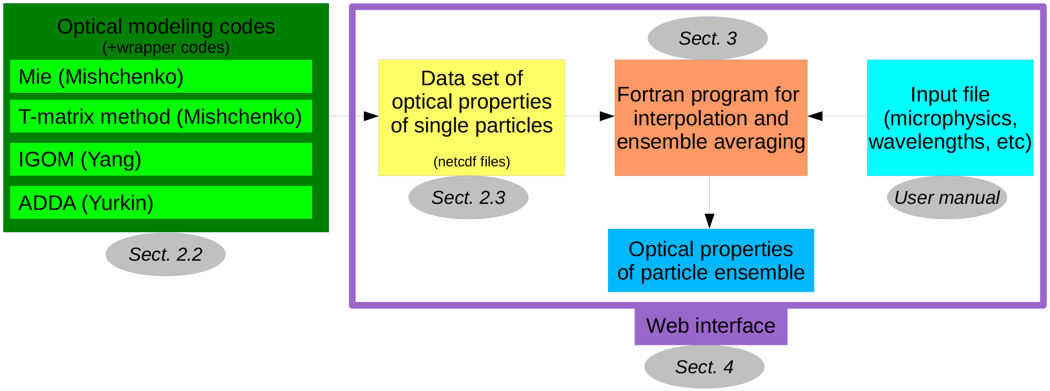
Figure 1Scheme of the MOPSMAP package, including the optical modeling codes applied to create the data set.
Aerosol particles in the Earth's atmosphere are important in various ways, for example because of their interaction with electromagnetic radiation and their effect on cloud properties. Consequently aerosol particles are relevant for weather and climate. The temporal and spatial variability in their abundance as well as the variability in their properties is significant which poses huge challenges in quantifying their effects. This includes the need to establish extended networks of observations using instruments such as photometers (Holben et al., 1998), lidars (Pappalardo et al., 2014), or ceilometers (Wiegner et al., 2014) and the development of models to predict the influence of particles on the state of the atmosphere; see, e.g., Baklanov et al. (2014).
Aerosol properties and distributions are often quantified by ground-based and spaceborne optical remote sensing and by optical in situ measurements. These measurements are indirect with respect to microphysical properties (e.g., particle size) because they measure optical quantities and require the application of inversion techniques to retrieve microphysical properties. Precise knowledge on the link between microphysical and optical properties is needed for the inversion. This link is provided by optical modeling, i.e., the optical properties of particles are calculated based on their microphysical properties. Optical modeling is required also for other applications, e.g., for radiative transfer, numerical weather prediction, and climate modeling. As optical modeling can be very time-consuming, it is often inevitable to pre-calculate optical properties of particles and store them in a lookup table, which is then accessed by the inversion procedures or subsequent models.
In our contribution we describe the MOPSMAP (Modeled optical properties of ensembles of aerosol particles) package, which consists of a data set of pre-calculated optical properties of single aerosol particles, a Fortran program which calculates the properties of user-defined aerosol ensembles from this data set, and a user-friendly web interface for online calculations. Figure 1 illustrates the overall scheme of the package, including the optical modeling codes (green box) needed once to prepare the underlying data set. MOPSMAP is either provided via an interactive web interface at https://mopsmap.net or via download as an offline application. The former is possible as MOPSMAP is computational very efficient. Compared to other data sets with predefined aerosol components, such as OPAC (Hess et al., 1998), compared to existing online Mie tools such as the one provided by Prahl (2018), and compared to GUI tools such as MiePlot Laven (2018), MOPSMAP is more flexible with respect to the characteristics of the aerosol ensembles. Moreover, our data set considers not only spherical particles but also spheroids and a small set of irregularly shaped dust particles. The output includes ASCII tables for further evaluation, netCDF files for direct application in the radiative transfer model uvspec (Emde et al., 2016), and plots, e.g., for educational purposes.
In Sect. 2, after defining aerosol properties, we describe how existing optical modeling codes were applied (green box in Fig. 1) to create the optical data set of single particles (yellow box). Subsequently, in Sect. 3, we describe the Fortran program (orange box) that uses this data set to calculate optical properties of user-defined particle ensembles. The web interface for online application of the MOPSMAP package is introduced in Sect. 4. To demonstrate the potential of MOPSMAP, several applications are discussed in Sect. 5 before we sum up our paper and give an outlook.
The optical properties of a particle with known microphysical properties are calculated by optical modeling. For the creation of the basic data set of MOPSMAP, optical modeling of single particles has been performed. In this section, we first define microphysical and optical properties of single particles and then describe how we created the data set using existing optical modeling codes.
We emphasize that the data set is, in principle, applicable to the complete electromagnetic spectrum; however, we use, for simplicity, the term “light” and consequently “optics” instead of more general terms.
2.1 Definition of particle properties
The description of particle properties is well-established and can be found in textbooks with varying levels of detail. Thus, we can restrict ourselves to a brief summary of those properties that are of special relevance for MOPSMAP.
The microphysical properties of an aerosol particle are described by its shape, size, and chemical composition.
Atmospheric aerosols might be spherical in shape but many types consist of nonspherical particles, often with a large variety of different shapes. Mineral dust (e.g., Kandler et al., 2009) and volcanic ash aerosols (e.g., Schumann et al., 2011b) are important examples of the latter, but, for example, pollen, dry sea salt or soot particles are also usually nonspherical. A quite common approach to consider the particle shape is the approximation using spheroids or distributions of spheroids (Hill et al., 1984; Mishchenko et al., 1997; Kahn et al., 1997; Dubovik et al., 2006; Wiegner et al., 2009). Spheroids originate from the rotation of ellipses about one of their axes. Only one parameter is required for the shape description. Mishchenko and Travis (1998) use the “axial ratio” ϵm, which is the ratio between the length of the axis perpendicular to the rotational axis and the length of the rotational axis. By contrast, Dubovik et al. (2006) use the “axis ratio” ϵd, defined as the inverse of ϵm. Spheroids with ϵm<1, ϵd>1 are called prolate (elongated) whereas spheroids with ϵm>1, ϵd<1 are oblate (flat) spheroids. The aspect ratio ϵ′ is the ratio between the longest and the shortest axis, i.e., in the case of prolate spheroids and in the case of oblate spheroids. Spheroids with are spheres.
The size of a particle is commonly described by its radius or diameter. While this is unambiguous in the case of spheres, more detailed specifications are necessary for any kind of nonspherical particles. Often the size of an equivalent sphere is used for the description of the nonspherical particle size: the volume-equivalent radius rv of a particle with known volume V (containing the particle mass, i.e., without cavities) is
whereas the cross-section-equivalent radius rc of a particle with known orientation-averaged geometric cross section Cgeo is
In the case of spheroids, rc is equal to the radius of a sphere having the same surface area (as used by Mishchenko and Travis, 1998). For the conversion between rv and rc, the radius conversion factor
is used (Gasteiger et al., 2011b). ξvc is equal to 1 in the case of spheres and decreases with increasing deviation from a spherical shape. Another definition of size is given by the radius of a sphere that has the same ratio between volume and geometric cross section as the particle
This definition corresponds to the case “VSEQU” presented by Otto et al. (2011), to the “effective radius” in Eq. (5) of Schumann et al. (2011a), and is more sensitive to non-sphericity than rv or rc. For example, a particle with rc=1 µm and ξvc=0.9 implies that rv=0.9 µm and rvcr=0.729 µm.
For setting up a data set of optical properties for different wavelengths, it is highly beneficial to make use of the size parameter
The size parameter x describes the particle size relative to the wavelength λ. The advantage of using x is that optical properties (qext, ω0, and F, as defined below) at a given wavelength are fully determined by its shape, refractive index m, and x. Equivalent size parameters xv, xc, and xvcr are calculated from the equivalent radii, analogously to Eq. (5).
The chemical composition of a particle determines its complex wavelength-dependent refractive index m. The imaginary part mi is relevant for the absorption of light inside the particle, whereby an imaginary part of zero corresponds to non-absorbing particles.
The optical properties of a nonspherical particle depend on the orientation of the particle relative to the incident light. In our data set we assume that particles are oriented randomly; thus, the optical properties are stored as orientation averages (Mishchenko and Yurkin, 2017).
The orientation-averaged optical properties at a given wavelength are fully described by the extinction cross section Cext, the single-scattering albedo ω0 and the scattering matrix F(θ), where θ is the angle by which the incoming light is deflected during the scattering process (“scattering angle”). The extinction cross section Cext can be normalized by the orientation-averaged geometric cross section Cgeo of the particle giving the extinction efficiency
The single-scattering albedo ω0 is given by
where Csca is the scattering cross section.
For the scattering matrix F of randomly oriented particles, we use the notation of Mishchenko and Travis (1998), i.e.,
with six independent matrix elements. The scattering matrix describes the transformation of the incoming Stokes vector Iinc to the scattered Stokes vector Isca:
where the Stokes vectors (van de Hulst, 1981) have the shape
and R is the distance of the observer from the particle. The Stokes vectors I describe the polarization state of light, with the first element I describing its total intensity. Thus, F is relevant for the polarization of the scattered light, and its first element a1, which is known as the phase function, is important for the angular intensity distribution of the scattered light. The phase function is normalized such that
For many applications it is useful to expand the elements of the scattering matrix using generalized spherical functions (Hovenier and van der Mee, 1983; Mishchenko et al., 2016). The scattering matrix elements at any scattering angle θ are then determined by a series of θ-independent expansion coefficients , , , , , and , with index l from 0 to lmax, see Eqs. (11)–(16) in Mishchenko and Travis (1998). lmax depends on the required numerical accuracy as well as on the scattering matrix itself. For example, in the case of strong forward scattering peaks (typically occurring at large x), lmax needs to be larger than in the case of more flat phase functions, to get the same accuracy.
The asymmetry parameter g is an integral property of the phase function:
g is the average cosine of the scattering angle of the scattered light and is calculated from the expansion coefficients by
2.2 Optical modeling of single particles
Depending on the particle type, different approaches are available for calculating particle optical properties. For the creation of the MOPSMAP optical data set, we use the well-known Mie theory (Mie, 1908; Horvath, 2009) in the case of spherical particles, which is a numerically exact approach over a very broad range of sizes. For spheroids we use the T-matrix method (TMM), which is a numerically exact method but limited with respect to maximum particle size. For larger spheroids not covered by TMM, we apply the improved geometric optics method (IGOM). For irregularly shaped particles the discrete dipole approximation (DDA) is applied.
2.2.1 Mie theory
We use the Mie code developed by Mishchenko et al. (2002) for optical modeling of spherical particles. In contrast to the nonspherical particle types described below, we do not store the optical properties of single particles (in a strict sense) because the properties of spheres can be strongly size-dependent, which would require a very high size resolution of our data set (e.g., Chýlek, 1990). Instead, we store data averaged over very narrow size bins, allowing us to use a lower size resolution resulting in a smaller storage footprint of the data set. For each size parameter grid point x, we actually consider a size parameter bin covering the range from to and apply the Mie code for 1000 logarithmically equidistant sizes within that bin before these results are averaged and stored.
2.2.2 T-matrix method (TMM)
We use the extended precision version of the code described by Mishchenko and Travis (1998) for modeling optical properties of spheroids. To improve the coverage of the particle spectrum (x, ϵm, and m), internal parameter values of the TMM code, which primarily determine the limits of the convergence procedures, were increased (NPN1 = 290; NPNG1 = 870; NPN4 = 260) as discussed by Mishchenko and Travis (1998). Though, in general, the TMM provides exact solutions for scattering problems, nonphysical results might be obtained due to numerical problems. To reduce the probability of nonphysical results and to increase the accuracy of the results, the parameter DDELT, i.e., the absolute accuracy of computing the expansion coefficients, was set to 10−6 (default 10−3). In non-converging cases, which occurred near the upper limit of the covered size range, the requirements were relaxed to DDELT = 10−3. Cases that did not converge even with the relaxed DDELT were not included in the data set. Nevertheless, some nonphysical results were obtained by this approach, for example, ω0>1, or outliers of otherwise smooth ω0(x) or g(x) curves. Thus, for plausibility checks for each particle shape and refractive index, single-scattering albedos ω0 and asymmetry parameters g were plotted over size parameter x and outliers were recalculated with slightly modified size parameters. Recalculations with nonphysical results were not included in the data set, which reduces the upper limit of the covered size range for that particular particle shape and refractive index.
2.2.3 Improved geometric optics method (IGOM)
Optical properties of large spheroids were calculated with the improved geometric optics method (IGOM) code provided by Yang et al. (2007) and Bi et al. (2009). In general, this approximation is most accurate if the particle and its structures are large compared to the wavelength. In addition to reflection, refraction, and diffraction by the particle, which are considered by classical geometric optics codes, IGOM also considers the so-called edge effect contribution to the extinction efficiency qext (Bi et al., 2009). Classical geometric optics results in qext=2, whereas qext is variable in the case of IGOM. The default settings of the code were used. The minimum size parameter was selected depending on the maximum size calculated with TMM.
2.2.4 Discrete dipole approximation code ADDA
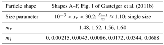
Natural nonspherical aerosol particles, such as desert dust particles, comprise practically an infinite number of particle shapes; thus, it is impossible to cover the full range of shapes in aerosol models. Moreover, the shape of each individual particle is never known under realistic atmospheric conditions. Consequently, typical irregularities such as flat surfaces, deformations or aggregation of particles can be considered only in an approximating way. To enable the user of MOPSMAP to investigate the effects of such irregularities the properties of six exemplary irregular particle shapes, as introduced by Gasteiger et al. (2011b), are provided. The geometric shapes were constructed using the object modeling language Hyperfun (Valery et al., 1999). The first three shapes are prolate spheroids with varying aspect ratios (A: ; B: ; C: ) and surface deformations according to Gardner (1984). Shape D is an aggregate composed of 10 overlapping oblate and prolate spheroids; surface deformations were applied as for shapes A–C. Shape E and F are edged particles with flat surfaces and a varying aspect ratio.
The optical properties were calculated with the discrete dipole approximation code ADDA (Yurkin and Hoekstra, 2011). A large number of particle orientations needs to be considered for the determination of orientation-averaged properties. ADDA provides an optional built-in orientation averaging scheme in which the calculations for the required number of orientations is done within a single run. An individual ADDA run using this scheme requires approximately the time for one orientation multiplied with the number of orientations (typically a few hundred), which can result in computation times of several weeks for large x. Because of the long computation times we split them up and performed independent ADDA runs for each orientation. The orientation-averaged properties are calculated in a subsequent step using the ADDA results for the individual orientations (see below).
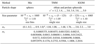
Table 1Microphysics of spheres and spheroids considered in the MOPSMAP data set.
* IGOM was not applied to m≤1.0.
Table 2Microphysics of irregularly shaped particles considered in the MOPSMAP data set.
The computational demand of DDA calculations increases strongly with size parameter x, typically with about x5 to x6. Thus, when aiming for large x, which is required for mineral dust in the visible wavelength range, it is necessary to find code parameters and an orientation averaging approach that provide a compromise between computation speed and accuracy.
The ADDA code mainly allows the following code parameters to be optimized:
-
DDA formulation
-
stopping criterion of the iterative solver
-
number of dipoles per wavelength.
We estimate the accuracy of the ADDA results by comparing orientation-averaged qext, qsca, a1(0∘), a1(180∘), and with results obtained using more strict calculation parameters. Accuracy tests are performed for shapes B and C, for size parameters xv=10.0, 12.0, 14.4, 17.3, 19.0, and 20.8, and for refractive index ; i.e., 12 single particle cases are considered in total. By comparing the different DDA formulations available in ADDA, it was found that the filtered coupled-dipole technique (ADDA command line parameter “-pol fcd -int fcd”), as introduced by Piller and Martin (1998) and applied by Yurkin et al. (2010), offers the best compromise between computation speed and accuracy of modeled optical properties. Using a stopping criterion for the iterative solver of 10−4 instead of 10−3 only has negligible influence on optical properties (<0.1 %) but requires approximately 30 % more computation time; thus, we used 10−3 for the ADDA calculations to create our data set. The extinction efficiency qext and the scattering efficiency qsca change in all cases by less than 0.3 % if a grid density of 16 dipoles per wavelength is used instead of 11. The maximum relative changes due to the change in dipole density are 0.2 % for a1(0∘), 1.7 % for a1(180∘), and 1.9 % for . Because of the large difference in computation time, which is about a factor of 3–4, and the low loss in accuracy, about 11 dipoles per wavelength were selected for the MOPSMAP data set. For xv<10 we use the same dipole set as for xv=10 so that the number of dipoles per wavelength increases with decreasing xv, being about 110∕xv.
The particle orientation is specified by three Euler angles (αe, βe, γe) as described by Yurkin and Hoekstra (2011) and basically a step size of 15∘ is applied for βe and γe resulting in 206 independent ADDA runs for each irregular particle. The orientation sampling and averaging is described in detail in Sect. S1.1 of the Supplement.
To test the accuracy of the selected orientation averaging scheme, orientation-averaged optical properties for shapes B, C, D, and F were compared to results using a much smaller step of 5∘ for βe and γe. These calculations consider about 12 times more orientations than the calculations used for MOPSMAP. Details are presented in Sect. S1.2 of the Supplement. Maximum deviations of less than 1 % are found for qext, qsca, and a1(0∘). For backscatter properties, a1(180∘) and , typical deviations are of the order of a few percent (max. 14 %). Moreover, in Sect. S1.3 of the Supplement, the selected orientation averaging scheme is applied to spheroids, and their optical properties are compared to reference TMM results. These deviations are comparable to those given in Sect. S1.2.
In summary, ADDA with the filtered coupled-dipole technique, at least 11 dipoles per wavelength and a stopping criterion for the iterative solver of 10−3 was used for optical modeling of the irregularly shaped particles in our data set together with the orientation averaging scheme combining 206 ADDA runs. Tests demonstrate that the modeling accuracy is mainly determined by the applied orientation averaging scheme.
2.3 Optical data set
Using the codes with the settings described above, a data set of modeled optical properties of single particles in random orientation was created. For spheres, we stored averages over narrow size bins as described above instead of single particle properties. An overview over the wide range of sizes, shapes, and refractive indices of the particles in the data set is given in Tables 1 and 2. For each combination of refractive index and shape a separate netCDF file was created, e.g., “spheroid_0.500_1.5200_0.008600.nc” for spheroids with ϵm=0.5 (prolate with ) and . Each file contains the optical properties on a grid of size parameters. The complete data set requires about 42 gigabytes of storage capacity.
For spheres and spheroids the minimum size parameter is set to 10−6, and the maximum size parameter is set to x≈1005 to cover, e.g., rc=80 µm at λ=500 nm. The size increment is 1 % (i.e., ) in the case of spheres, 5 % in the case of TMM spheroids, and 10 % for IGOM spheroids. In the case of spheroids having refractive indices most relevant for atmospheric studies, the TMM is applied up to (or close to) the largest possible size parameter with the approach described in Sect. 2.2.2. The maximum size parameter of the TMM calculations is reduced for less relevant refractive indices. An overview is given in Sect. S2 of the Supplement and a detailed list of the maximum size parameters for all m and ϵm combinations can be downloaded from Gasteiger and Wiegner (2018). The maximum size parameter for TMM is in the range , strongly depending on m and particle shape, and determines the lowest size parameter at which IGOM may be applied. The first IGOM size parameter is between 0 and 10 % larger than the maximum TMM size parameter. The TMM and IGOM results for spheroids are merged into a single netCDF file covering the complete size range from to x≈1005, which is sufficient for most applications. For example, for prolate spheroids with and , the size range from to x=88.22 is covered by TMM; IGOM starts at x=89.54. The transition from TMM to IGOM for several scattering angles is demonstrated in Sect. S3 of the Supplement. Since IGOM is an approximation, unrealistic jumps of optical properties may occur at the transition. For typical mineral dust ensembles in the visible spectrum, particles in the IGOM range contribute less than 10 % to the total extinction. IGOM was not applied to mr<1.04; thus, the size parameter range is limited to the TMM range for these refractive indices. A step of 0.04 was selected for the mr grid in the most relevant range (from 1.00 to 1.68) and a wider mr step elsewhere. The development of the data set started with mi=0.0043, and beginning from this value, mi was increased and decreased in steps of a factor . Below mi=0.001 and above mi=0.1, the step width is a factor of 2.
The optical data for the irregularly shaped particles (Table 2) are limited to xv≤30.2 because of the huge computation requirements for optical modeling of large particles. Nonetheless, the most important range for many applications is covered; e.g., at λ=1064 nm particles up to rv=5.1 µm can be modeled. The m grid for the irregularly shaped particles is limited to the most relevant range for desert dust in the visible spectrum, and the mi step is set to a factor of 2. The quantification of the conversion factor ξvc of the six irregular shapes requires the determination of their orientation-averaged geometric cross sections, which is done numerically.
The optical properties stored for each particle are the extinction efficiency qext, the scattering efficiency qsca, and the expansion coefficients , , , , , and of the scattering matrix. The ADDA and the IGOM code provide the angular-resolved scattering matrix elements, which we converted to the expansion coefficients stored in the data set following the method described by Hovenier and van der Mee (1983) and Mishchenko et al. (2016). We optimized the expansion coefficients for accurate scattering matrices at 180∘, which is probably the most error sensitive angle. As a by-product, lidar applications will certainly benefit from this optimization.
In the case of asymmetric shapes in random orientation, the scattering matrix has 10 independent elements as discussed by van de Hulst (1981). By using only six elements of F (Eq. 8) in our data set, we implicitly assume that each irregular model particle (shapes A–F) occurs as often as its mirror particle, which is formed by mirroring at a plane (van de Hulst, 1981).
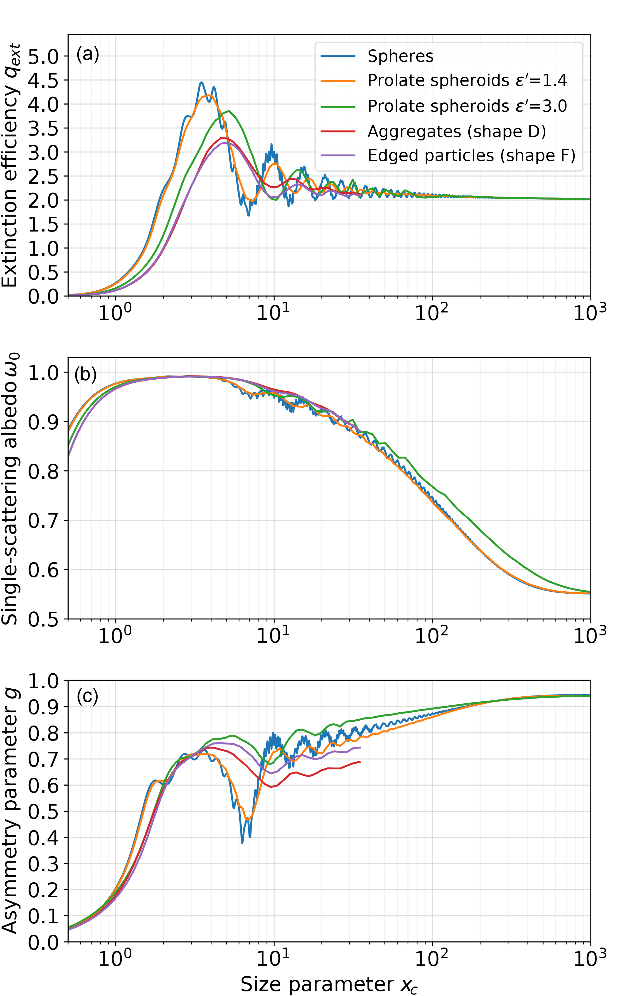
Figure 2Optical properties of single particles (or narrow size bins in the case of spheres) with fixed refractive index as a function of size parameter. The different colors denote different particle shapes. Panel (a) shows the extinction efficiency qext, panel (b) the single-scattering albedo ω0, and panel (c) the asymmetry parameter g.
Figure 2 shows an example from the MOPSMAP optical data set. The refractive index is set to , which is representative of desert dust particles at visible wavelengths. The properties of spherical particles are shown in blue, whereas the properties of prolate spheroids with and 3.0 are shown in orange and green, respectively. Red and violet lines denote irregularly shaped particles D and F, respectively. Figure 2a shows the extinction efficiency qext as a function of cross-section-equivalent size parameter xc. The general shape of the qext(xc) curve is similar for the different shapes; nonetheless, with increasing deviation from a spherical shape, the amplitudes of the oscillations of qext(xc) become smaller and a shift in the maximum qext towards larger xc is found. Figure 2b shows the single-scattering albedo ω0 for the same particles as Fig. 2a. For particle sizes comparable to the wavelength, ω0 reaches maxima with values of about 0.991, almost independent of particle shape. ω0 approaches a value of about 0.551 at xc≈1000 for spheres and spheroids. Fig. 2c shows the asymmetry parameter g. When the particle size becomes comparable to the wavelength, g increases and oscillates as a function of xc, with the strongest oscillations occurring in the case of spheres. There is some shape dependence of g for xc>5; in particular, the aggregate shape results in systematically smaller g than the other shapes for xc>10. The transition from the numerically exact TMM to the IGOM approximation occurs at xc≈125 for (orange line) and at xc≈27 for (green line) and is quite smooth.
In this section the basic characteristics of the MOPSMAP Fortran program to calculate optical properties of particle ensembles are described. Besides a modern Fortran compiler, e.g., gfortran 6 or above, the netCDF Fortran development source code is required to build the executable. The computation time and memory requirements depend on the ensemble complexity and the number of wavelengths but in general are low for state-of-the-art personal computers. The Fortran code and the data set are available for download from Gasteiger and Wiegner (2018), and a web interface (see Sect. 4) provides online access to most of the functionality of the Fortran program without the requirement of downloading the code and the data set.
Within each MOPSMAP run the optical properties of a specific user-defined ensemble are calculated at a user-defined wavelength grid. The ensemble microphysics and the wavelength grid are defined in an input file. The details about the options available for the input file are described in a user manual which is provided together with the code.
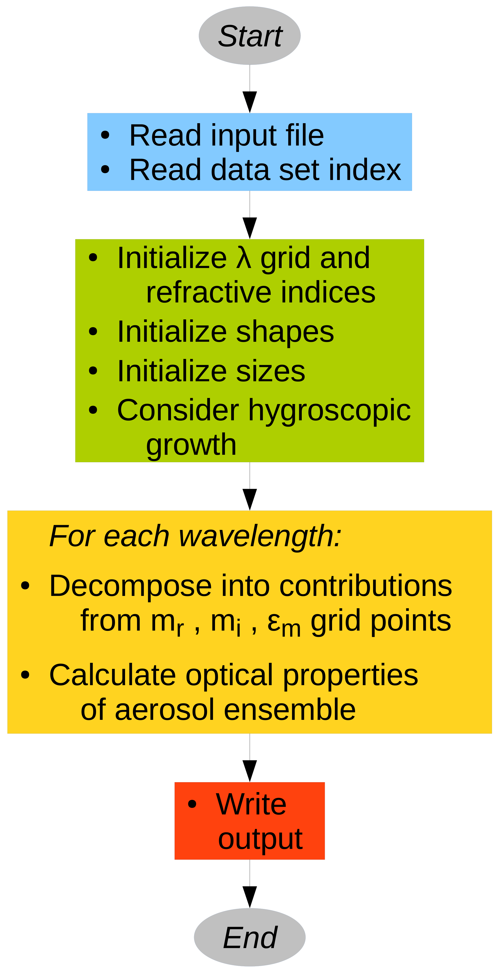
Figure 3 shows a flow chart of the MOPSMAP Fortran program. The program is initialized by reading the input file and a data set index. The latter contains information on the refractive index and shape grid and the size parameter ranges covered by the data set. Then, all information required for the optical modeling is initialized, for example the set of wavelengths, the refractive indices as a function of wavelength, shape distributions, and the effect of the hygroscopic growth, before the optical calculations are performed for each wavelength, as described in the following.
3.1 Calculation of optical properties of particle ensembles
Usually aerosol particles occur as ensembles of particles of different size, refractive index, and/or shape. The different particles contribute to the optical properties of the ensemble. Assuming that the distance between the particles is large enough for interaction of light with each particle to occur without influence from any other particle (“independent scattering”; van de Hulst, 1981), the contribution of each particle can be added as described below.
In MOPSMAP particle ensembles are composed of one or more independent modes (the terms “mode” and “component” are often used synonymously in the literature). Each mode in MOPSMAP is characterized by particle size, shape, and refractive index, whereby each property can be described as a fixed value or as a distribution (see below). As these parameters do not necessarily correspond to the grid points of the MOPSMAP data set, for each mode (and each wavelength), decomposition into contributions from the different available m and shapes of the data set needs to be performed.
For a mode containing spheroids, in the most simple but probably most frequently used case of fixed values of mr, mi, and ϵm, linear interpolation in the three-dimensional (mr, mi, ϵm) space of the MOPSMAP data set is performed; i.e., eight grid points contribute to the result, with each grid point weighted according to the normalized distance from the parameters of the mode. For each dimension, the contributing grid points are the nearest grid point smaller or larger than the value of the mode; e.g., for the real part of the refractive index mr
The weight of the grid points mr,i and is
Finally the weights for each of the eight contributions are calculated as the products of the weights determined for each dimension. An example is shown in Sect. S4 of the Supplement. The error in the interpolation of the user-specified values between the grid points of the data set is discussed in Sect. 3.3
Under other conditions more or less than eight contributions have to be considered. In the case of spheres or a single irregular shape, an interpolation in the shape dimension is not necessary, so that four contributions are sufficient. In the case of a spheroid aspect ratio distribution, contributions from all required ϵm grid points are considered and weighted according to the given distribution. In the case of a mode containing a non-absorbing fraction (see below), an additional mi grid point, mi=0, may be required. Furthermore, because of the limited size range of irregularly shaped particles in the data set, a special treatment can be applied: a MOPSMAP option is available which substitutes irregularly shaped particles above a selected size parameter with other particle shapes, spherical or nonspherical, as selected by the user. As a consequence, the particle shape of that mode becomes size- and wavelength-dependent and the number of different contributions increases. The total number of contributions for an ensemble, denoted as J in the following, varies because the number of modes is not fixed and, as just discussed, the number of contributions from each mode depends on the characteristics of each mode. This underlines the flexibility of MOPSMAP.
The optical properties of the particle ensemble are calculated for each wavelength by summation over extensive properties of all particles described by the J contributions. This approach corresponds to the so-called external mixing of particles. Each contribution has a size distribution nj(r), i.e., a particle number concentration per particle radius interval from r to r+dr, in the range from to , which is obtained by multiplying the user-defined size distribution of the mode with the weights obtained during the decomposition. The extinction coefficient αext and the scattering coefficient αsca are calculated by
The expansion coefficients need to be weighted with Csca,j(r); for example, of a particle ensemble is calculated by
For the integration of extensive properties over the size distribution, we apply the trapezoidal rule, which assumes linearity between the r grid points.
The size distribution for each mode can be specified in various ways. The MOPSMAP user can either specify a single size, apply size distribution tables in ASCII format, or apply a size distribution parameterization. The following parameterizations are available:
-
– log-normal distribution;
-
– modified gamma distribution, Deirmendjian (1964);
-
– exponential distribution, α=0, γ=1;
-
n(r)=Arα – power law distribution, Junge distribution, B=0, Deirmendjian (1964);
rmod is the mode radius, σ a dimensionless parameter for the relative width of the distribution, and N0 the total number density (in the range from to ) of the lognormal distribution. For the subsequent size distributions, parameters A, α, B, and γ are positive and A controls the scaling of total number density whereas α, B, and γ are relevant for the shape of the size distributions. The exponential distribution, power law distribution, and the gamma distribution are a subset of the modified gamma distribution with the specific parameter values as given above (see also Petty and Huang, 2011).
The particle shape can be specified independently for each mode and is, within each mode, independent of size and refractive index. In the case of spheroids, either a fixed aspect ratio ϵ′ or an aspect ratio distribution is used. The latter can be given as a table in an ASCII file or it can be parameterized by a modified lognormal distribution (Kandler et al., 2007)
with parameters for the location of the maximum of n(ϵ′) and σar for the width of the distribution.
The refractive index of each mode can either be wavelength-independent or specified as a function of wavelength in an ASCII file. In addition, it is possible to specify for each mode a non-absorbing fraction 𝒳. If 𝒳>0, the mode is divided, for all sizes and shapes, into a non-absorbing (, relative abundance 𝒳) and an absorbing fraction (, relative abundance 1−𝒳). As a consequence, the average mi over all particles of the mode remains equal to the mi as specified by the user. This non-absorbing fraction approach can be used as a parameterization of the refractive index variability within desert dust ensembles as described by Gasteiger et al. (2011b) and below in Sect. 5.6.
For the hygroscopic particle growth the following parameterization (Petters and Kreidenweis, 2007; Zieger et al., 2013)
is implemented in MOPSMAP, where RH is the relative humidity and κ the hygroscopic growth parameter of the particles of each mode. This equation describes the ratio between the size of the particle at a given RH and the size of the particle in a dry environment (RH=0 %). The parameterization implies that this ratio is independent of size; thus, for example in the case of a lognormal size distribution, rmin, rmax, and rmod are multiplied with this ratio, whereas the relative width σ of the distribution is not modified. This is the usual approach though modal representations of aerosol size distributions may also predict higher moments (Binkowski and Shankar, 1995; Zhang et al., 2002), and thus σ can be a prognostic variable as well. The refractive index is modified by the water taken up following the volume weighting rule. Both RH and κ can be chosen by the user. This parameterization is valid for particles with r>40 nm, where the Kelvin effect can be neglected (Zieger et al., 2013). It is worth noting that this parameterization differs from the relative humidity dependence implemented in OPAC, which was adapted from Hänel and Zankl (1979).
3.2 Output of Fortran program
As output of MOPSMAP the following properties of aerosol ensemble are available. Redundant properties, such as lidar-related properties, are available to facilitate the use of the results:
-
extinction coefficient αext (m−1)
-
single-scattering albedo ω0
-
asymmetry parameter g
-
effective radius (µm) (referring to rc, rv, or rvcr as selected by the user)
-
number density N (m−3) (number of particles per atmospheric volume)
-
cross section density a (m−1) (particle cross section per atmospheric volume)
-
volume density v (particle volume per atmospheric volume)
-
mass concentration M (gm−3) (particle mass per atmospheric volume)
-
expansion coefficients ( to ) for elements of scattering matrix
-
scattering matrix elements (a1 to b2) at user defined angle grid
-
volume scattering function () at user defined angle grid
-
backscatter coefficient ()
-
lidar ratio (sr)
-
linear depolarization ratio
-
Ångström exponents for
-
extinction-to-mass conversion factor (g m−2)
-
mass-to-backscatter conversion factor ().
Scattering matrix elements and the quantities derived from them are calculated from the expansion coefficients. Wavelength-independent properties reff, N, a, v, and M are calculated for each wavelength to demonstrate the numerical accuracy of the integration.
The results are available in ASCII and in netCDF format. The format of the program output is described in the user manual. The netCDF output files can be read by the radiative transfer model uvspec, which is included in libRadtran (Mayer and Kylling, 2005; Emde et al., 2016).
3.3 Interpolation and sampling error
Due to the limited size resolution in the data set and required interpolations between refractive index and aspect ratio grid points, deviations from exact model calculations for specific microphysical properties occur. As examples, Fig. 4 illustrates deviations introduced for single particle properties, whereas Table 3 shows deviations for particle ensembles.
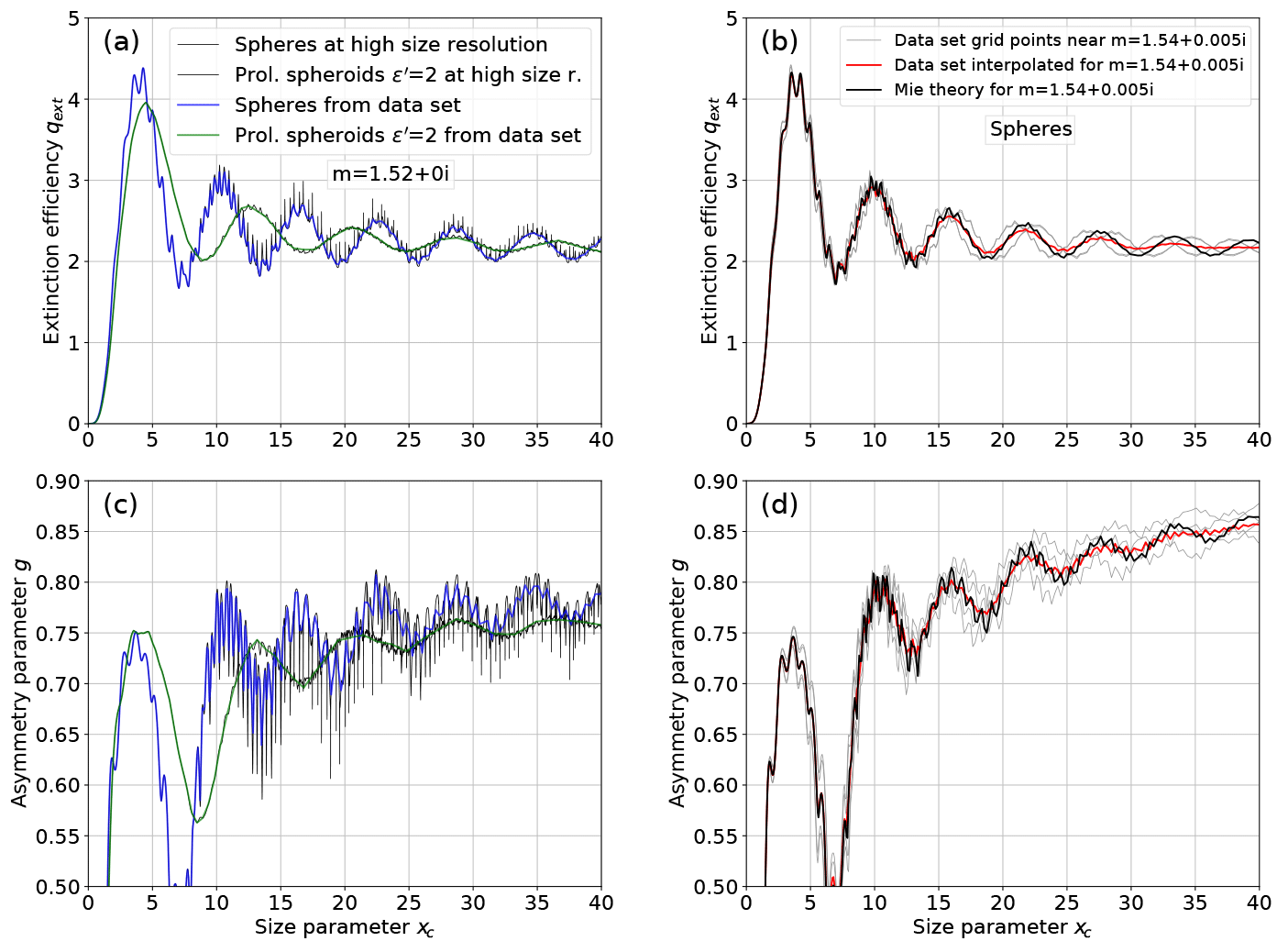
Figure 4Examples illustrating the effect of the limited size resolution of the MOPSMAP data set (a, c) and the effect of the interpolation between the refractive index grid points of the data set (b, d); extinction efficiencies qext (a, b) and asymmetry parameters g (c, d) as functions of the size parameter from x=0 to x=40 are compared; in (a) and (c) the high size-resolution calculations (black lines) were performed with linear x steps of 0.002 in the case of spheres and 0.01 in the case of spheroids; in (b) and (d) the red lines show properties calculated with MOPSMAP for by interpolation between refractive indices included in the data set (i.e., between , , , and , for which the properties are shown as thin gray lines), and for comparison, the black lines show the properties calculated by Mie theory explicitly for using the same x grid as used by the data set.
Table 3Optical properties calculated for a lognormal mode with rmod=0.5 µm, σ=2.0, µm, and µm at λ=628.32 nm. Two cases of particle shapes are considered: spheres and prolate spheroids with . The columns “data set” contain values calculated using MOPSMAP with the data set described in Sect. 2.3. For comparison, the same properties are calculated in the columns “highres” using a high size resolution and in the columns “explicit” using Mie theory or TMM explicitly at .
In Fig. 4a and c effects of the limited size resolution on the extinction efficiency qext and the asymmetry parameter g are shown for non-absorbing spheres and spheroids with . In particular for spheres with x>10, deviations for single particles can be considerable because of small-scale features that are not resolved in the data set. In the case of spheres these features are implicitly considered in the data set by storing the average over 1000 sizes within each size bin as described above. In the case of spheroids, the data set contains properties calculated for single sizes which may not be fully representative of close-by sizes. However, since the small-scale features are much weaker for spheroids than for spheres, the average deviation for spheroids is much smaller than for spheres.
In Fig. 4b and d effects due to the required interpolation between the refractive index grid points are illustrated for spheres with . While the red lines show the properties calculated from the data set, the black lines show Mie calculations done explicitly for with the same size grid as used in the data set. The comparison illustrates that MOPSMAP calculates optical properties on average correctly, but some smaller-scale features are lost: for example, the extinction efficiency qext(x) in the size parameter range from 20 to 40 is dampened compared to the Mie calculation for because of the interference of the qext(x) curves for mr=1.52 and mr=1.56 (see gray lines in Fig. 4b; note that curves for different mi lie almost on top of each other).
For other size ranges, refractive indices, and optical quantities, the effects on the single particle properties are in principle similar but they may vary in magnitude.
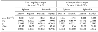
Table 3 investigates the sampling and interpolation errors for a mono-modal lognormal size distribution with a typical width of σ=2.0. The effective radius is reff=1.44 µm, which is a typical value for transported desert aerosol. Sizes up to µm, which corresponds to size parameter xc=40 at λ=628.32 nm, are considered. The left half of Table 3 compares optical properties calculated from the MOPSMAP data set (columns “data set”) with properties calculated using a high size resolution (columns “highres”), the same resolutions as displayed in Fig. 4a. For spheres, the results are equal up to at least the fourth digit. In the case of prolate spheroids with , deviations are found for the fourth digit of αext and g. For the lidar-related quantities S and δl, the differences are larger with the relative deviation of δl being 2.6 %. These differences are caused by the high sensitivity of lidar-related quantities, and it is expected that deviations become smaller when shape distributions or wider size distributions are applied.
The right half of Table 3 demonstrates the effect of the m interpolation for an exemplary . MOPSMAP calculations (columns “data set”) are compared to results obtained using explicitly this refractive index in the Mie and TMM calculations. While the effect of the m interpolation is very small for αext, g, and δl, it is slightly larger for ω0 and S. The maximum relative effect is found for the lidar ratio S of spheres with a deviation of 1.7 %.
These comparisons demonstrate that deviations found for single particles are largely smoothed out in the case of particle ensembles due to the averaging over a large number of different particles. Only for a few special atmospheric applications, for example, the modeling of a rainbow, the limited resolution of the data set may still lead to a considerable error.
A web interface is provided as part of MOPSMAP at https://mopsmap.net. It was designed to be intuitive for expert and nonexpert users, e.g., for the demonstration of sensitivities of optical properties on microphysical properties in the framework of lectures, but also for a lot of scientific problems as outlined in the following section. The web interface is written in PHP and uses the SQLite library. After the registration as a user, online calculations of optical properties of a large range of particle ensembles can be performed. Input and output can be defined by the user; for nonexpert users, a lot of default ensembles representative of specific climatological conditions are already available. The input parameters primarily include the microphysical properties of the particles. The particles' microphysics are described by up to four components (each described by an individual lognormal size distribution), the wavelength dependence of the refractive index and the shape. Any lognormal size distribution can be used; to facilitate the usage (e.g., for nonexpert users), the aerosol components from the OPAC data set (Hess et al., 1998), e.g., “mineral coarse mode”, “water-soluble”, or “soot”, are already included. The same is true for the 10 “aerosol types” defined in OPAC, e.g., “continental clean”, “urban” or “maritime polluted”, consisting of a combination of components. Calculations can be made for a single wavelength, for wavelength ranges or a prescribed wavelength set (e.g., for a typical aerosol lidar or a AERONET sun photometer). Moreover, users can define their own wavelength sets, e.g., for a specific radiometer. The relative humidity is selected by the user and it is effective for all hygroscopic components according to Eq. (21). The hygroscopic growth of the OPAC components in MOPSMAP differs from the original OPAC version (Hess et al., 1998); it follows the κ parameterization with the values proposed by Zieger et al. (2013). In the “expert user mode” the flexibility is further increased: the number of components can be larger than four, and the size distribution can be given as discrete values on a user-defined size grid.

Figure 5Properties of OPAC aerosol types as a function of relative humidity RH calculated with the κ parameterization (Zieger et al., 2013) implemented in MOPSMAP (Eq. 21). The different colors denote the 10 different OPAC aerosol types as indicated in the legends. The columns denote different wavelengths λ as indicated above the upper row. The upper row shows the extinction coefficient normalized to the extinction coefficient of the same aerosol type at RH =0 % and λ=532 nm. The single-scattering albedo ω0, the extinction-to-mass conversion factor η, and the mass-to-backscatter conversion factor Z are plotted in the subsequent rows.
The output comprises the complete set of optical properties as described in Sect. 3.2. It can be downloaded for further applications and includes ASCII tables as well as a netCDF file that can be used for radiative transfer calculations with uvspec of the widely used libRadtran package (Emde et al., 2016). To provide an immediate overview over the results, the most important parameters, such as extinction coefficient (αext), single-scattering albedo (ω0), asymmetry parameter (g), Ångström exponent (AE), or lidar ratio (S), are displayed as tables when the calculations have been completed. In addition plots of the results as a function of wavelength and scattering angle are shown as selected by the user.
All results are stored in the user's personal folder so that all calculations can be reproduced. Furthermore, all calculations can also easily be rerun with a slightly modified input parameter set.
In this section a selection of examples is presented to demonstrate the wide range of applications of MOPSMAP. Many of them can be performed by using the web interface. Some examples need a local version of MOPSMAP alongside with scripts that repeatedly call the Fortran program. These scripts are written in Python and can be downloaded from Gasteiger and Wiegner (2018) as part of the MOPSMAP package.
It is worth mentioning that numerous studies demonstrate the need for optical modeling of aerosol ensembles, thus illustrating the range of possible applications of MOPSMAP. Moreover, optical modeling is essential for many different related modeling activities. It is required, for example, for closure experiments (consistency checks between different measurement methods involving an aerosol model, e.g., Wiegner et al., 2009; Gasteiger et al., 2011b; Müller et al., 2012; Bell et al., 2013; Ma et al., 2014; Zieger et al., 2014; Düsing et al., 2018), radiative transfer studies (e.g., Otto et al., 2009; Emde et al., 2010), the inversion of remote-sensing measurements (e.g., Dubovik et al., 2006; Gasteiger et al., 2011a; Müller et al., 2016), the inversion of in situ data (e.g., Weinzierl et al., 2009; Szymanski et al., 2009; Kassianov et al., 2014), aerosol layer visibility simulations (e.g., Weinzierl et al., 2012), dynamic aerosol transport models (e.g., Heinold et al., 2007; Balzarini et al., 2015), aerosol characterization (e.g., Gasteiger et al., 2017; Che et al., 2018; Zhuang et al., 2018), and solar energy (e.g., Polo et al., 2016; Kosmopoulos et al., 2017).
5.1 Effect of hygroscopicity
The first example of applications deals with hygroscopic growth. If aerosol particles are hygroscopic, their microphysical and optical properties change with RH. Fig. 5 shows how optical properties of the 10 OPAC aerosol types (Hess et al., 1998), which contain up to four components, some of which are hygroscopic, change with RH. These calculations were performed using the MOPSMAP web interface, where the OPAC aerosol types are available as predefined ensembles and the relative humidity can be chosen by the user. MOPSMAP considers the hygroscopic effect by application of the κ parameterization (Eq. 21), which differs from the RH dependency implemented in OPAC.
The upper row of Fig. 5 shows the normalized extinction coefficient of the different types (indicated by color) at three wavelengths λ (each in a subplot) calculated for RH values of 0, 50, 70, 80, and 90 %. The extinction at all λ is normalized to the extinction at RH =0 % and λ=532 nm. As a consequence, the differences between the columns illustrate the wavelength dependency of the extinction, whereas changes with RH illustrate the hygroscopic effects. For example, for the desert aerosol type (orange color), the wavelength dependency is low, which is related to the large size of the dominant mineral particles, and the hygroscopic effect is relatively weak because mineral particles are hygrophobic. By contrast, for maritime (bluish colors) and antarctic types (purple color), the wavelength dependence is stronger and the hygroscopic effect is strong because of the domination by highly hygroscopic sulfate and sea salt particles. For the continental as well as the urban and arctic types, the wavelength dependence is even stronger and the hygroscopic effect weaker, which may be explained by strong contributions from the soot and water-soluble components which contain quite small particles with κ values significantly smaller than the κ values of sea salt particles (e.g., Petters and Kreidenweis, 2007; Markelj et al., 2017; Enroth et al., 2018; Psichoudaki et al., 2018).
The single-scattering albedo ω0 is shown in the second row of Fig. 5. ω0 varies strongly with aerosol type, with the highest values of almost 1.0 for the antarctic, maritime clean, and maritime tropical aerosol types. Since water is almost non-absorbing at the considered wavelengths, the water uptake hardly changes ω0 if ω0 is already close to 1.0. The single-scattering albedo of the desert type is much lower, but it is also virtually independent on the RH as this aerosol type does not take up much water. For the other types, an increase in RH results in an increase in ω0.
The extinction-to-mass conversion factor η, which is plotted in the third row of Fig. 5, is necessary to calculate mass concentrations from extinction coefficient measurements or mass loadings from AOD measurements. An important parameter for η is the particle size (e.g., Gasteiger et al., 2011a) with the consequence that the desert aerosol type, which contains the highest fraction of coarse particles of the considered types, shows the highest η values. Again, the wavelength dependency is significant for the other aerosol types so that the η values at λ=1064 nm (right column) are significantly larger than at λ=532 nm (middle column). The dependence of η on RH is significantly weaker than the dependence of the extinction on RH (upper row), which may be explained by the increase in mass with increasing RH compensating for the increase in extinction.
The bottom row of Fig. 5 illustrates the mass-to-backscatter conversion factor Z as a function of RH. Z is useful, for example, for comparisons of vertical profiles simulated with aerosol transport models to profiles measured with lidar or ceilometer. The multiplication of simulated aerosol mass concentration M with Z provides simulated β profiles which can be compared with the measurements. The figure shows that there is considerable spread between the different aerosol types, in particular at short wavelengths. RH only has strong effects on the maritime and arctic aerosol types.
Currently the hygroscopic growth of different aerosol components is not ultimately understood, and different κ-values are discussed. With MOPSMAP their influence on the optical properties can easily be determined and used in validation studies.
5.2 Optical properties for sectional aerosol models
Aerosol transport models in combination with the optical properties of the aerosol allow one to model the radiative effect of the aerosol. The aerosol is typically modeled in terms of mass concentrations for a limited number of aerosol types divided over a few size bins (sectional aerosol model) or a few modes (modal aerosol models). Thus, realistic optical properties for each size bin of each aerosol type are required for modeling the radiative effects (e.g., Curci et al., 2015).
Table 4Optical properties at λ=500 nm of the five COSMO-MUSCAT dust size bins. Two cases for the particle shape are considered: spheres∕prolate spheroids. For details, see text.
In this example, we calculated the optical properties of dust at λ=500 nm for the five size bins of the COSMO-MUSCAT model (Heinold et al., 2007). The size bins are determined by the radius limits 0.1, 0.3, 0.9, 2.6, 8, and 24 µm. We assumed constant dv∕dlnr within each bin. Each bin was modeled through the expert mode of the MOPSMAP web interface. The refractive index is , which is equal to the value given for the mineral components in OPAC. We considered two cases for the particle shape: on the one hand, spherical particles and, on the other hand, prolate spheroids with the aspect ratio distribution given by Kandler et al. (2009). For the latter case we assumed volume-equivalent sizes to keep the particle mass constant.
The calculated phase functions are presented in Fig. 6, where each size bin is represented by an individual color. The difference between both lines of the same color represents the shape effect. For size bin 1 (0.1 µm µm, black lines), the difference is small, whereas for all other bins the shape effect is larger. The strongest effects are found for with differences of up to a factor of 4 between the particle shapes. These angular ranges can be important, for example, for the backscattering of sunlight into space and thus for the aerosol radiative effect. The very strong effect at is relevant for any lidar application, e.g, the intercomparison of modeled and measured attenuated backscatter profiles (Chan et al., 2018).

Figure 6Phase functions at λ=500 nm of the five COSMO-MUSCAT dust size bins (different colors) assuming spherical particles (solid lines) and prolate spheroids (dashed lines). For details, see text.
Calculated parameters relevant for radiative transfer and remote sensing are given in Table 4. The shape effect on the single-scattering albedo ω0 and the asymmetry parameter g is small except for size bin 2 where g is significantly larger for the spheroids than for the spheres. The extinction-to-mass conversion factor η is systematically smaller for spheroids than for spheres in bins 2–5 because the geometric cross section of the spheroids is ≈5.5 % larger than the cross section of the volume-equivalent spheres. The mass-to-backscatter conversion factor Z of the spheroids is lower than the Z of spheres for most size bins, with maximum differences being larger than a factor of 2.
5.3 Effect of cutoff at maximum size
Many in situ measurement setups are limited with respect to the maximum particle size they are able to sample, e.g., because of losses at the inlet or the tubing. In this example, we illustrate the effect of the cutoff for the desert aerosol type from OPAC at RH =0 % (Koepke et al., 2015).
Table 5Properties of one-modal size distribution at λ=532 nm consisting of spheres or aggregate particles (shape D, ξvc=0.8708; Fig. 1 of Gasteiger et al., 2011b) assuming different size equivalences. For details, see text.
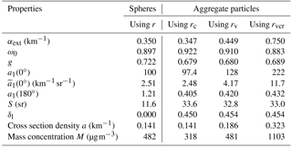

Figure 7Optical and microphysical properties of the OPAC desert aerosol type as a function of cutoff radius rmax. Panel (a) shows the normalized extinction coefficient αext at three wavelengths, the normalized cross section density a, and the normalized mass concentration M. Normalization to values calculated for µm. The single-scattering albedo ω0 at the same wavelengths is plotted in (b), and the asymmetry parameter g in (c).
Figure 7 illustrates various aerosol properties as a function of the cutoff radius rmax. Fig. 7a shows properties that are normalized by the values found at µm (where 99.988 % of the total particle cross section is covered, referring to ). The PM10 mass, i.e., the mass in the particles with diameter smaller than 10 µm ( µm), and the PM2.5 mass ( µm) are standard parameters to quantify pollution (e.g., Querol et al., 2004). In our example, PM10 and PM2.5 contain only 59.5 and 21.6 % of the total particle mass, respectively. However, PM10 and PM2.5 measurement setups cover 94.4 and 69.0 % of the total geometric cross section, respectively. The single-scattering albedo in the case of PM2.5 is about 0.035–0.071 higher than for the total aerosol, whereas the asymmetry parameter is reduced by about 0.02–0.04. As a further example, if the cutoff is µm, 97.8 % of the total cross section and 75.6 % of the mass are covered; the single-scattering albedo and the asymmetry parameter deviate from the total aerosol by less than 0.008.
This example shows that consideration of maximum size is essential when derived optical properties or mass concentrations are interpreted, and results can be severely misleading if the cutoff radius is not considered. These effects can be easily quantified with MOPSMAP and its web interface.
5.4 Effect of the selection of size equivalence of nonspherical particles
This example demonstrates how the selection of the size equivalence in the case of nonspherical particles affects various ensemble properties. In MOPSMAP the size-related parameters are either interpreted as rc (default) or as rv or rvcr (see Sect. 2.1) according to the choice of the user. Each size equivalence can be transformed into another by Eqs. (3) and (4). For example, if “volume cross section ratio equivalent” has been chosen in the web interface, and “0.5” for rmod, this would be equivalent to setting for rmod when the default “cross section equivalent” is kept (ξvc depending on shape).
To further elucidate the role of the different representations of radii, the same parameters of a lognormal size distribution are applied to the different size interpretations. For this purpose, the parameters are set to rmod=0.5 µm and σ=2 with µm, µm (reff=0.98 µm), and N0=103.66 cm−3, which results in a concentration of N=100 cm−3 in the range from rmin to rmax. The effect of the three alternative interpretations on particle size is demonstrated in Fig. 8 for irregular shape D having ξvc=0.8708. All three size distributions (curves of different color) are plotted in terms of dN∕drc(rc) (black axes). For comparison, axes for dN∕drv(rv) (red axes) and dN∕drvcr(rvcr) (green axes) are also shown. Using these axes, the size distribution curves can be interpreted in terms of the various size equivalences. The comparison between the size distributions clearly shows a shift towards larger sizes when rvcr or rv instead of rc is assumed. For example, assuming rvcr for the lognormal size distribution (green curve) describes the same ensemble as using µm µm =0.757 µm (see Eq. 4) and µm =2.65 µm when assuming rc as particle size.
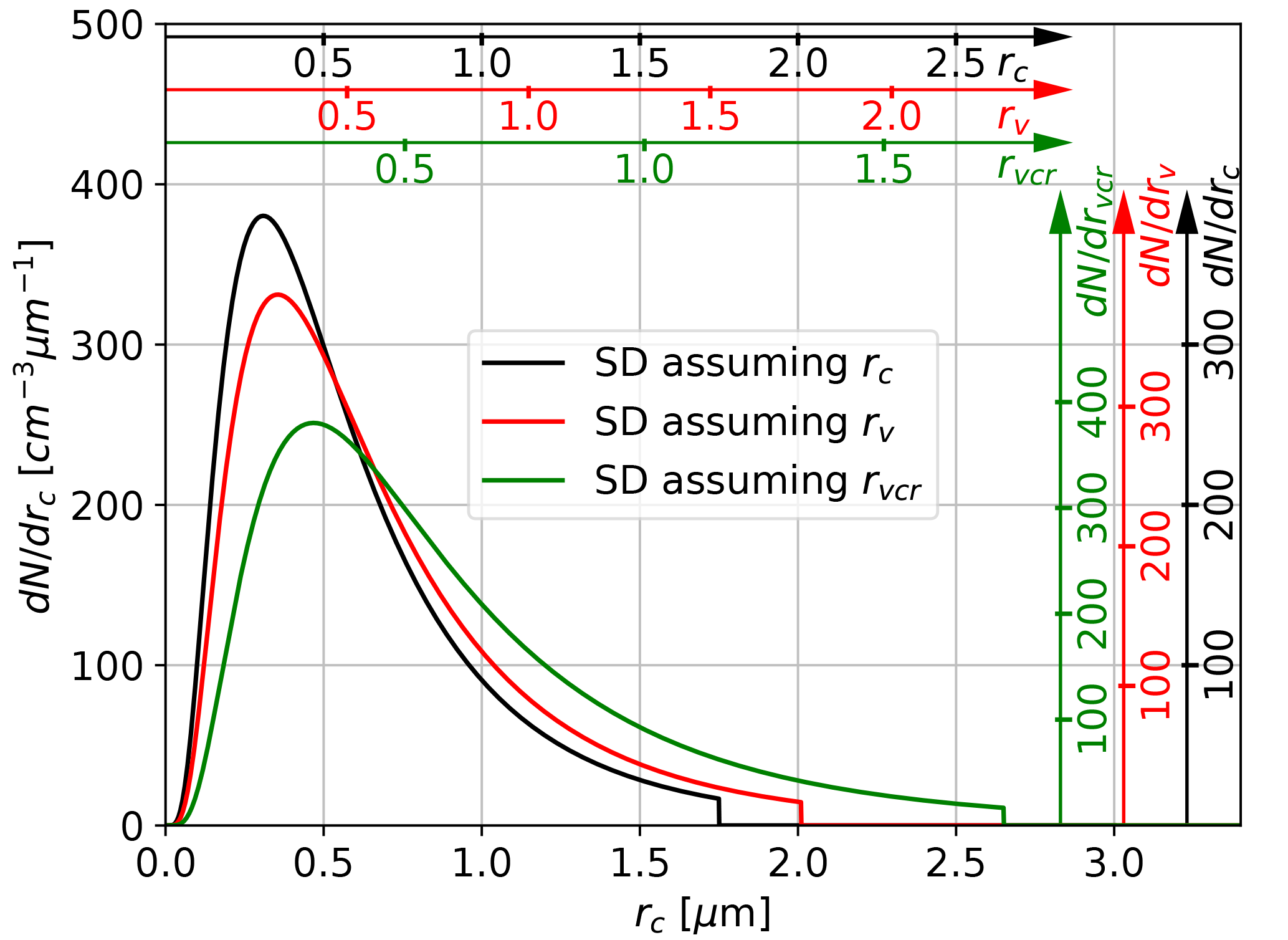
Figure 8Lognormal size distributions (SD) with same rmod, σ, N0, and rmax assuming different size equivalences for aggregate particles (shape D, ξvc=0.8708) as applied in Table 5. The size distributions are plotted in terms of cross-section-equivalent sizes (i.e., dN∕drc(rc) referring to black axes and grid). For comparison axes valid for the other size interpretations are also plotted in red and green, which allows each size distribution to be interpreted in terms of each size equivalence.
Since the size distributions depend on the selected size equivalence various (optical) properties of the ensemble are also different; a quantification has been provided by MOPSMAP (Table 5). The particle mass density is set to 2600 kg m−3, the refractive index is and the wavelength is λ=532 nm. The first column of Table 5 shows the optical properties of spherical particles. In the subsequent columns, all particles are assumed to be aggregate particles (shape D) with the same rc (second column, corresponding to the black curve in Fig. 8), the same rv (third column, red curve), and the same rvcr (last column, green curve) as the spheres in the first column.
The results are consistent with the increase in particle size from assuming rc over rv to rvcr (see cross section density a, mass concentration M, and also Fig. 8). The extinction coefficient αext and the forward volume scattering (0∘) of the nonspherical particles best agree with the spherical counterparts if cross section equivalence is assumed. These properties are known to be sensitive to the particle cross section for particles larger than the wavelength. The absorption is in first approximation proportional to the particle volume if absorption is weak. As a consequence, for the single-scattering albedo ω0, both cross section and volume are relevant and dependencies are more complicated than for αext. The single-scattering albedo ω0 of shape D decreases in Table 5 from left to right due to the strong increase in particle volume. The selection of the size equivalence has a small effect on the asymmetry parameter g, the backward phase function a1(180∘), the lidar ratio S, and the linear depolarization ratio δl.
These results highlight the importance of a thoughtful selection of the size equivalence. The most appropriate size equivalence certainly depends on the concept of how the size distribution is measured. For example, if scattering by coarse dust particles is measured and the size is inverted assuming spherical particles, assuming cross-section equivalence in subsequent applications with nonspherical particles seems natural as scattering mainly depends on the particle cross section. MOPSMAP and its web interface provides the flexibility to investigate this topic theoretically.
5.5 Uncertainty estimation of calculated optical properties
In general, the knowledge on microphysical properties is limited; thus, they are subject to uncertainties. If these uncertainties can be quantified, it is consistent to also quantify the corresponding uncertainties of the optical properties.
In this regard, the sensitivity of a calculated optical property ζ to changes in a microphysical property ψ is an important aspect that can be expressed by the first partial derivative . The Jacobian matrix J is the M×N matrix containing all first partial derivatives for M optical properties and N microphysical properties. The elements of J of an aerosol ensemble can be numerically calculated by perturbing the microphysical properties of the ensemble. For demonstration in the following example we perturb ψ with a factor of 0.99 and 1.01 to numerically calculate the first partial derivatives. A sample script for the calculation of J is provided together with MOPSMAP.
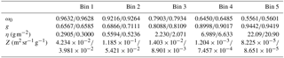
Table 6Elements of the Jacobian matrix, i.e., first partial derivatives, of a dust-like ensemble (see text for details).
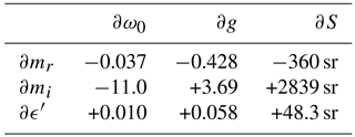
Table 6 shows an example of J for the optical properties and the microphysical properties . J was calculated for a simplified dust ensemble described by one lognormal size mode with rmod=0.1 µm, σ=2.6, µm, µm, a refractive index , and prolate spheroids with . The wavelength is set to λ=532 nm. This results in ω0=0.9020, g=0.7319, and S=69.95 sr. These properties are most sensitive to mi, which can be clearly seen from Table 6. For example, a change in mi by 0.001 would result in a change in ω0 of 0.011. An increase in ϵ′ or mi increases g and S, whereas an increase in mr reduces their values. The sensitivity to perturbations of the microphysical properties is particularly strong for the lidar ratio S, which can be seen by comparing S=69.95 sr of the ensemble with the partial derivatives. We emphasize that the accuracy of J is limited by the sampling in the MOPSMAP data set (see also Sect. 3.3); for example, partial derivatives are constant between the mr grid points of the data set.
The Jacobian matrix J is valid for a certain set of microphysical properties values and, as mentioned, J can be used to quantify the uncertainty of the calculated properties for a given microphysical uncertainty. However, when uncertainties in the microphysical properties become larger, J may change significantly within the uncertainty range of ψ and other approaches may be required to estimate the uncertainty in the calculated optical properties. A simple approach applicable to this problem is the Monte Carlo method (e.g., JCGM, 2008). Repeated calculations with microphysical properties randomly chosen within the uncertainty range are performed. The uncertainty of the calculated quantities is determined by the statistics over the different sampled ensembles. In general, the computation time is longer than using J and is proportional to the number of calculated ensembles. Due to the statistical nature of the Monte Carlo method, the final results get more precise with increasing number of sampled ensembles. A script for the Monte Carlo uncertainty propagation is provided together with MOPSMAP. For example, based on the ensemble described above, sampling within the uncertainty ranges µm, , , , and results in the ranges , , and 29 sr 103 sr.
5.6 Effect of refractive index variability
Mineral dust aerosols are ensembles of different minerals with different refractive indices. Usually the variability in the refractive index of the particles within a dust aerosol ensemble is neglected when modeling its optical properties. In this example, we compare optical properties calculated using the full measured variability in the imaginary part of the refractive index mi to properties calculated with the common assumption of all particles in an ensemble having an average mi. Furthermore, a parameterization of the variability is considered.
We use the desert aerosol type of OPAC (Koepke et al., 2015). Prolate spheroids with the aspect ratio distribution of Kandler et al. (2009) are assumed for the mineral components and spherical particles for the WASO component (RH =0 %). The real part of the refractive index is mr=1.53 for all particles. The wavelength in this example is set to λ=355 nm, which is a wavelength where absorption by iron oxide is strong. Because of the variable iron oxide content of individual particles, the variability in mi is large at this wavelength. Consequently, a significant influence on optical properties can be expected. In this example we consider three cases of imaginary part variability: first, we apply the size-resolved distribution of the imaginary part of the refractive index for Saharan dust as derived from mineralogical analysis (Kandler et al., 2011). Second, we assume the average imaginary part for all particles (it is 0.0175, which is close to 0.0166 given for the mineral components in OPAC at λ=355 nm). Finally, we parameterize the mi distribution with the non-absorbing fraction approach as introduced in Sect. 3.1. In this case, we set 𝒳=0.5, resulting in 50 % of the mineral particles having mi=0, whereas the other 50 % of the particles have mi=0.0349.
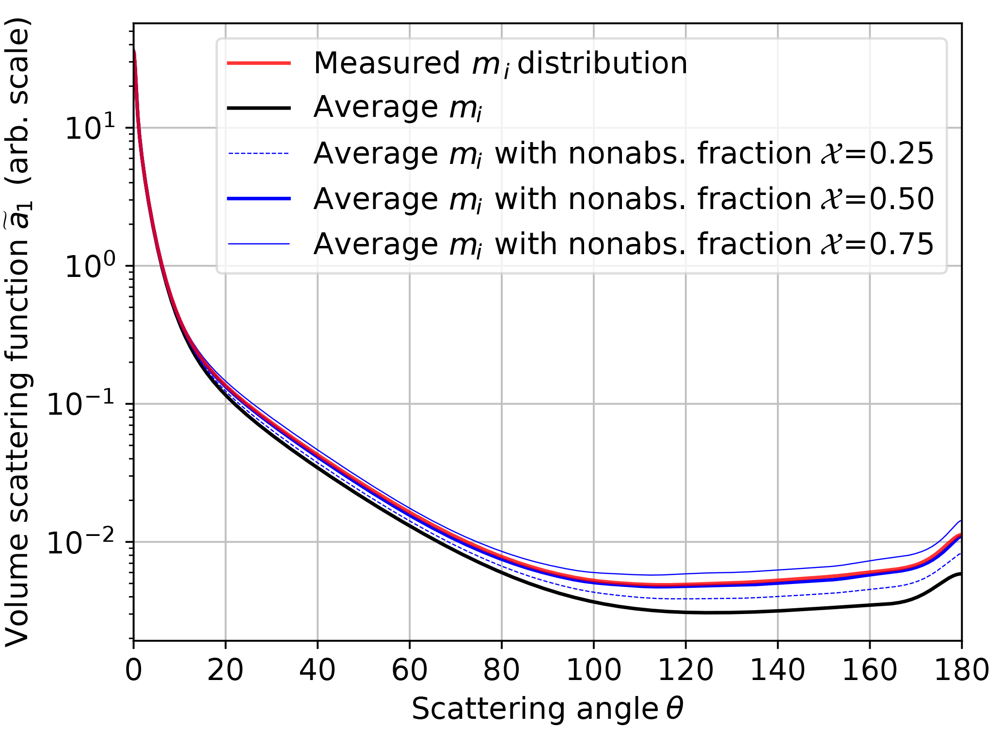
Figure 9Volume scattering function of dust at λ=355 nm (arbitrary scale) using either the mi distribution (red) measured by Kandler et al. (2011), the average mi of these measurements (black), or applying the non-absorbing fraction parameterization with different 𝒳 (blue).
Figure 9 shows the volume scattering function for the three cases. This figure shows that the sensitivity of the forward scattering to the mi distribution is negligible whereas the sensitivity increases with increasing scattering angle θ. For backward scattering, the difference between the measured mi distribution (red line) and using the average mi (black line) is more than a factor of 2. The parameterization assuming 𝒳=0.5 (thick blue line) is in much better agreement with the measured case. The root-mean-square relative deviation between the volume scattering function for the measured distribution and for the average mi is 30 %, whereas it is only 4 % for the parameterization. For comparison two additional 𝒳 values, i.e., 𝒳=0.25 (thin dashed blue line) as well as 𝒳=0.75 (thin solid blue line), are also shown in Fig. 9, but their deviation is larger than for the parameterization with 𝒳=0.5. The extinction coefficient αext only changes by less than 0.03 % between the three representations of mi. For ω0 we obtain 0.852 using the measured mi distribution, whereas ω0=0.741 when using the average mi and ω0=0.834 using the parameterization with 𝒳=0.5. For the asymmetry parameter g, we obtain 0.744, 0.789, and 0.749 for the measured, averaged, and parameterized cases, respectively. For the lidar ratio S, values of 41, 78, and 42 sr are calculated for the three cases, whereas for the linear depolarization ratio δl values of 0.241, 0.212, and 0.220 are obtained.
These results emphasize that it is important to consider the nonuniform distribution of the absorptive components in the desert dust ensembles for optical modeling of such aerosols at short wavelengths. We have shown in this example that optical properties of Saharan dust can be well simulated with 𝒳=0.5. Whether this conclusion holds for other cases of desert dust can easily be investigated by means of MOPSMAP when measurements of mi distributions of further dust types are available.
5.7 Effect of particle shape on the nephelometer truncation error
Integrating nephelometers aim to measure in situ the total scattering coefficient of aerosol particles by detecting all scattered light. The angular sensitivities of real nephelometers, however, deviate from the ideal sensitivity, which is the sine of scattering angle θ. For example, nearly forward or nearly backward scattered light does not reach the detectors because of the instrument geometry (Müller et al., 2011). This has to be considered during the evaluation of measurements and can be done by applying a truncation correction factor to the measured scattering coefficients . Cts can be calculated theoretically using optical modeling if aerosol microphysical properties and the angular sensitivity of the instrument are known. Some nephelometers not only measure the total scattering coefficient but also the hemispheric backscattering coefficient, which is the scattering integrated from θ=90 to 180∘. For the hemispheric backscattering coefficient, a correction factor also needs to be applied to correct the measured hemispheric backscattering coefficient affected by the nonideal instrument sensitivity. This correction factor Cbs is defined analogously to Cts as the ratio between the true coefficient and the measured one. Note that this hemispheric backscattering coefficient is defined differently from β, which is measured by lidars and used elsewhere in this paper.
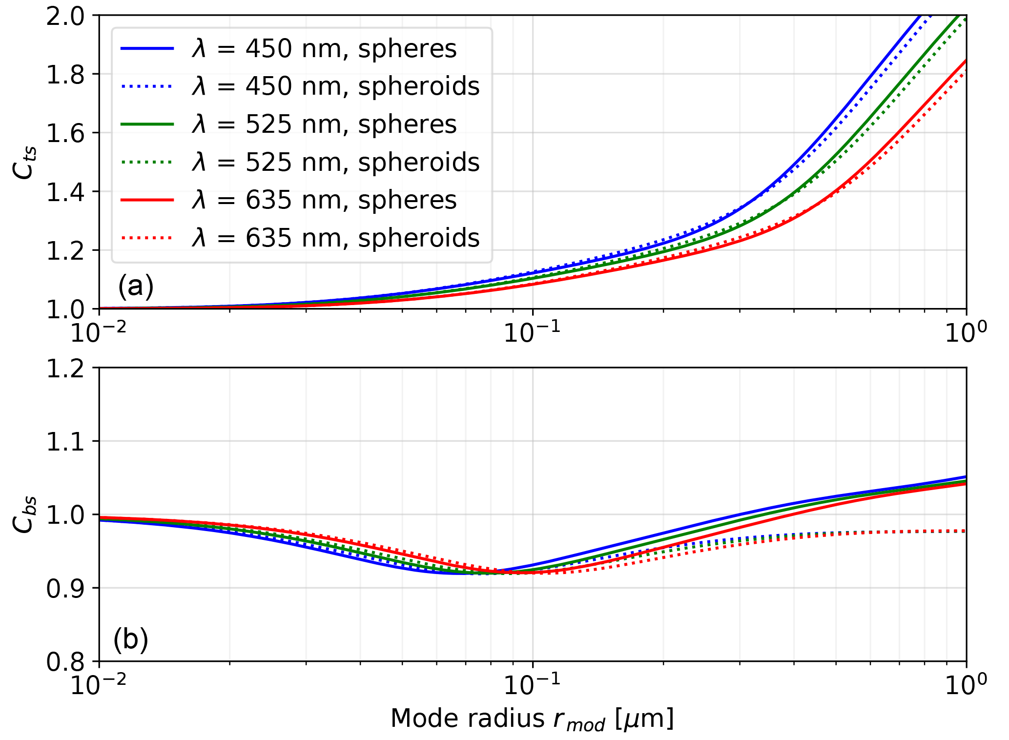
Figure 10Modeled correction factors Cts for total scattering (a) and Cbs for hemispheric backscattering (b) of an Aurora 3000 nephelometer as a function of particle size. For details, see text.
Figure 10 shows modeled correction factors for the total (Fig. 10a) and the backscatter (Fig. 10b) channel of an Aurora 3000 nephelometer. The angular sensitivity of the instrument is taken from Müller et al. (2011). For the following sensitivity study the mineral dust refractive index from OPAC (Hess et al., 1998), the parameterized mi distribution with 𝒳=0.5 (as shown in Sect. 5.6), a lognormal size mode with σ=1.6 and a maximum radius of µm (corresponding to a PM10 inlet) is assumed. The mode radius rmod is varied from 0.01 to 1 µm (horizontal axis) and two cases for the particle shape, i.e., spherical particles (solid lines) and cross-section-equivalent prolate spheroids with the ϵ′ distribution from Kandler et al. (2009) (dashed lines), are considered. The colors denote the three operating wavelengths of the instrument (450, 525, and 635 nm). The figure shows that the total scattering correction factor Cts mainly depends on particle size. In the case of large particles (rmod=1 µm), the nephelometer underestimates total scattering by a factor of ≈2 if the truncation error is not corrected. Shape only has a small effect on forward scattering; thus, its influence on the correction of the truncation error is less than 3 % (compare dashed and solid lines of the same color). The maximum shape effect on Cbs is 7 %, i.e., indicating that assuming spherical particles for the truncation correction may result in an overestimation of the hemispheric backscattering coefficient.
The correction factors might be recalculated for example when new data on the refractive index or particle shape become available. This example highlights the potential of MOPSMAP as a useful tool for the characterization of optical in situ instruments. In addition, it could be used for the interpretation of angular measurements, for example, as performed with a polar photometer by Horvath et al. (2006).
5.8 Optical properties of ash from different volcanoes close to the source
Vogel et al. (2017) present a data set comprising shape–size distributions of ashes from nine different volcanoes as well as wavelength-dependent refractive indices for five different ash types. The particles were collected between 5 and 265 km from the volcanoes. While refractive indices can also be expected to be valid at larger distances from the volcanoes, the effective radii in the range from 9.5 to 21 µm are probably not realistic for long-range-transported ash. Based on this data set, which is available in the supporting information of Vogel et al. (2017), we calculate optical properties of these volcanic ashes with MOPSMAP. Each single particle is modeled as a prolate spheroid with the given size and aspect ratio, as well as with the refractive index given for the type of ash the volcano emits. In addition, we assume a non-absorbing fraction of 𝒳=0.5 (as used in Sect. 5.6). The application of this non-absorbing fraction approach seems reasonable when taking into account the variability in the transparency of the particles shown in Fig. 5 of Vogel et al. (2017). Due to the data set limits of MOPSMAP, particles with r>47.5 µm are modeled as r=47.5 µm and aspect ratios >5 are set to 5. For each volcano, less than 0.5 % of the particles was affected by these modifications.

Figure 11Modeled wavelength-dependent optical properties for ashes from different volcanoes. More details on the ash samples are given in Table 1 of Vogel et al. (2017). The colors indicate ash type: basalt is dark blue, basaltic andesite is light blue, andesite is green, dacite is orange, and rhyolite is red (see Fig. 7 of Vogel et al., 2017 for reference).
Figure 11 shows the single-scattering albedo ω0 and the asymmetry parameter g for the nine ashes as a function of wavelength between 300 and 1500 nm. Differences of ω0 are up to about 0.12 with ash from Chaitén (Chile) and Mt. Kelud (Indonesia) being the least and most absorbing species, respectively. ω0 is correlated with the ash type, which is mainly a result of the significant variability in mi (see Fig. 16b of Vogel et al., 2017). For all ashes, ω0 increases slightly with wavelength, typically by about 0.05 over the wavelength range shown. The variability in g is less than 0.05, and for all ashes the changes with wavelength are weak with values of less than 0.02. The mass-to-backscatter conversion factor Z varies between 1.16 and for the nine ashes. The extinction-to-mass conversion factor η at λ=550 nm ranges from 14.8 to 33.0 g m−2 which is considerably higher than known for typical aerosols (e.g., Fig. 5) or volcanic ash transported over continental scales (e.g., η between 1.10 and 1.88 g m−2 found by Wiegner et al., 2012). In particular the different values of η clearly demonstrate that optical properties of volcanic ash layers drastically change with the distance from the eruption due to changing microphysics.
This example suggests that it is worthwhile considering the specific microphysical properties of each volcano. However, for realistic MOPSMAP calculations valid in the long-range regime, size distributions different from the ones used in this example must certainly be applied whereas the refractive indices are more likely representative.
Radiative properties of atmospheric aerosols are relevant for a wide range of meteorological applications, in particular for radiative transfer calculations and remote-sensing and in situ techniques. Optical properties strongly depend on the microphysical properties of the particles – size, refractive index and shape – properties that are highly variable under ambient conditions. As a consequence, the application of mean properties could be questionable. However, the determination of optical properties of specific aerosol ensembles can be quite time-consuming, in particular when nonspherical particles shall be considered.
For this purpose we have developed the MOPSMAP package that provides the full set of optical properties of arbitrary, randomly oriented aerosol ensembles: single particles of the ensemble can be spherical or spheroidal with size parameters up to x≈1000. Moreover, a small set of irregular particles is considered. The refractive index can be and . The size distribution of the ensemble can either be parameterized as a lognormal distribution, as a (modified) gamma distribution, or freely chosen according to individual data. MOPSMAP includes a web interface for online calculations at https://mopsmap.net, offering the most frequently used options; for advanced applications or large sets of computations, the full package is freely available for download. Key applications of MOPSMAP are expected to be the evaluation of radiometer measurements in the UV, VIS and near-infrared spectral range or aerosol lidar measurements. They can help to improve the inversion of such measurements for aerosol characterization. Furthermore, MOPSMAP can be used to refine optical properties of aerosols in radiative transfer models or in numerical weather prediction and chemistry transport models.
The details of the concept underlying MOPSMAP are discussed in this paper. Several examples are presented to illustrate the potential of the package, including an example to calculate optical properties for sectional aerosol models and an example illustrating the effect of maximum size cutoff that occurs in the inlet system of in situ instruments. In another example, conversion factors between the backscatter coefficient (available from lidar/ceilometer measurements or from numerical forecast models) and the mass concentration of volcanic ashes have been calculated. These conversion factors are relevant to estimate flight safety after volcanic eruptions and vary by about a factor of 3 between the nine ashes under investigation.
The concept of MOPSMAP allows continuous upgrades to further extend the range of applications. For example, the resolution of the refractive index grid could be increased, new versions of underlying scattering codes could be applied when available, larger size parameters could be considered, e.g., using DDA for m close to 1 (Yurkin and Hoekstra, 2011), and new sets of irregular particles could be implemented, e.g., those presented by Mehri et al. (2018). However such extensions can be quite time-consuming, so that extensions are expected to be limited. Moreover, conceptional upgrades will be investigated without knowing yet whether they can be included in the web interface. Here, a trade-off between scientific complexity and user-friendliness must be found. Whereas internal mixing in the case of homogeneous particles is already covered in the present version, the implementation of a core-shell particle model can be discussed. Finally, we want to emphasize that the feedback from the users will help us to set up a priority list of further actions.
The MOPSMAP data set and the Fortran code, including scripts related to examples presented in this paper, are available at https://doi.org/10.5281/zenodo.1284217 (Gasteiger and Wiegner, 2018).
The supplement related to this article is available online at: https://doi.org/10.5194/gmd-11-2739-2018-supplement.
JG set up the database of optical properties and implemented the Fortran codes; MW developed the web interface. The paper was written by both, with JG drafting the paper.
The authors declare that they have no conflict of interest.
This project has received funding from the European Research Council (ERC)
under the European Union's Horizon 2020 research and innovation programme
(grant agreement no. 640458, A-LIFE). The authors thank Michael Mishchenko,
Ping Yang, and Maxim Yurkin for providing their optical modeling codes.
Thanks are due to Daniel Sauer, Sara Valentini, Marilena Teri, and Bernadett
Weinzierl for suggestions that helped to improve MOPSMAP.
Edited by: Klaus Gierens
Reviewed by: two
anonymous referees
Baklanov, A., Schlünzen, K., Suppan, P., Baldasano, J., Brunner, D., Aksoyoglu, S., Carmichael, G., Douros, J., Flemming, J., Forkel, R., Galmarini, S., Gauss, M., Grell, G., Hirtl, M., Joffre, S., Jorba, O., Kaas, E., Kaasik, M., Kallos, G., Kong, X., Korsholm, U., Kurganskiy, A., Kushta, J., Lohmann, U., Mahura, A., Manders-Groot, A., Maurizi, A., Moussiopoulos, N., Rao, S. T., Savage, N., Seigneur, C., Sokhi, R. S., Solazzo, E., Solomos, S., Sørensen, B., Tsegas, G., Vignati, E., Vogel, B., and Zhang, Y.: Online coupled regional meteorology chemistry models in Europe: current status and prospects, Atmos. Chem. Phys., 14, 317–398, https://doi.org/10.5194/acp-14-317-2014, 2014. a
Balzarini, A., Pirovano, G., Honzak, L., Žabkar, R., Curci, G., Forkel, R., Hirtl, M., José, R. S., Tuccella, P., and Grell, G.: WRF-Chem model sensitivity to chemical mechanisms choice in reconstructing aerosol optical properties, Atmospheric Environ., 115, 604 – 619, https://doi.org/10.1016/j.atmosenv.2014.12.033, 2015. a
Bell, S. W., Hansell, R. A., Chow, J. C., Tsay, S.-C., Hsu, N. C., Lin, N.-H., Wang, S.-H., Ji, Q., Li, C., Watson, J. G., and Khlystov, A.: Constraining aerosol optical models using ground-based, collocated particle size and mass measurements in variable air mass regimes during the 7-SEAS/Dongsha experiment, Atmos. Environ., 78, 163–173, https://doi.org/10.1016/j.atmosenv.2012.06.057, 2013. a
Bi, L., Yang, P., Kattawar, G. W., and Kahn, R.: Single-scattering properties of triaxial ellipsoidal particles for a size parameter range from the Rayleigh to geometric-optics regimes, Appl. Opt., 48, 114–126, https://doi.org/10.1364/AO.48.000114, 2009. a, b
Binkowski, F. S. and Shankar, U.: The Regional Particulate Matter Model: 1. Model description and preliminary results, J. Geophys. Res.-Atmos., 100, 26191–26209, https://doi.org/10.1029/95JD02093, 1995. a
Chan, K. L., Wiegner, M., Flentje, H., Mattis, I., Wagner, F., Gasteiger, J., and Geiß, A.: Evaluation of operational model forecasts of aerosol transport using ceilometer network measurements, Geosci. Model Dev. Discuss., https://doi.org/10.5194/gmd-2018-74, in review, 2018. a
Che, H., Qi, B., Zhao, H., Xia, X., Eck, T. F., Goloub, P., Dubovik, O., Estelles, V., Cuevas-Agulló, E., Blarel, L., Wu, Y., Zhu, J., Du, R., Wang, Y., Wang, H., Gui, K., Yu, J., Zheng, Y., Sun, T., Chen, Q., Shi, G., and Zhang, X.: Aerosol optical properties and direct radiative forcing based on measurements from the China Aerosol Remote Sensing Network (CARSNET) in eastern China, Atmos. Chem. Phys., 18, 405–425, https://doi.org/10.5194/acp-18-405-2018, 2018. a
Chýlek, P.: Resonance structure of Mie scattering: distance between resonances, J. Opt. Soc. Am. A, 7, 1609–1613, https://doi.org/10.1364/JOSAA.7.001609, 1990. a
Curci, G., Hogrefe, C., Bianconi, R., Im, U., Balzarini, A., Baró, R., Brunner, D., Forkel, R., Giordano, L., Hirtl, M., Honzak, L., Jiménez-Guerrero, P., Knote, C., Langer, M., Makar, P., Pirovano, G., Pérez, J., José, R. S., Syrakov, D., Tuccella, P., Werhahn, J., Wolke, R., Žabkar, R., Zhang, J., and Galmarini, S.: Uncertainties of simulated aerosol optical properties induced by assumptions on aerosol physical and chemical properties: An AQMEII-2 perspective, Atmos. Environ., 115, 541–552, https://doi.org/10.1016/j.atmosenv.2014.09.009, 2015. a
Deirmendjian, D.: Scattering and Polarization Properties of Water Clouds and Hazes in the Visible and Infrared, Appl. Opt., 3, 187–196, https://doi.org/10.1364/AO.3.000187, 1964. a, b
Dubovik, O., Sinyuk, A., Lapyonok, T., Holben, B. N., Mishchenko, M., Yang, P., Eck, T. F., Volten, H., Muñoz, O., Veihelmann, B., van der Zande, W. J., Leon, J., Sorokin, M., and Slutsker, I.: Application of spheroid models to account for aerosol particle nonsphericity in remote sensing of desert dust, J. Geophys. Res., 111, D11208, https://doi.org/10.1029/2005JD006619, 2006. a, b, c
Düsing, S., Wehner, B., Seifert, P., Ansmann, A., Baars, H., Ditas, F., Henning, S., Ma, N., Poulain, L., Siebert, H., Wiedensohler, A., and Macke, A.: Helicopter-borne observations of the continental background aerosol in combination with remote sensing and ground-based measurements, Atmos. Chem. Phys., 18, 1263–1290, https://doi.org/10.5194/acp-18-1263-2018, 2018. a
Emde, C., Buras, R., Mayer, B., and Blumthaler, M.: The impact of aerosols on polarized sky radiance: model development, validation, and applications, Atmos. Chem. Phys., 10, 383–396, https://doi.org/10.5194/acp-10-383-2010, 2010. a
Emde, C., Buras-Schnell, R., Kylling, A., Mayer, B., Gasteiger, J., Hamann, U., Kylling, J., Richter, B., Pause, C., Dowling, T., and Bugliaro, L.: The libRadtran software package for radiative transfer calculations (version 2.0.1), Geosci. Model Dev., 9, 1647–1672, https://doi.org/10.5194/gmd-9-1647-2016, 2016. a, b, c
Enroth, J., Mikkilä, J., Németh, Z., Kulmala, M., and Salma, I.: Wintertime hygroscopicity and volatility of ambient urban aerosol particles, Atmos. Chem. Phys., 18, 4533–4548, https://doi.org/10.5194/acp-18-4533-2018, 2018. a
Gardner, G. Y.: Simulation of natural scenes using textured quadric surfaces, Proceedings of the 11th annual conference on Computer graphics and interactive techniques, 11–20, 1984. a
Gasteiger, J. and Wiegner, M.: Modeling of aerosol optical properties with MOPSMAP: Fortran program with data set, https://doi.org/10.5281/zenodo.1284217, 2018. a, b, c, d
Gasteiger, J., Groß, S., Freudenthaler, V., and Wiegner, M.: Volcanic ash from Iceland over Munich: mass concentration retrieved from ground-based remote sensing measurements, Atmos. Chem. Phys., 11, 2209–2223, https://doi.org/10.5194/acp-11-2209-2011, 2011a. a, b
Gasteiger, J., Wiegner, M., Groß, S., Freudenthaler, V., Toledano, C., Tesche, M., and Kandler, K.: Modeling lidar-relevant optical properties of complex mineral dust aerosols, Tellus B, 63, 725–741, https://doi.org/10.1111/j.1600-0889.2011.00559.x, 2011b. a, b, c, d, e, f
Gasteiger, J., Groß, S., Sauer, D., Haarig, M., Ansmann, A., and Weinzierl, B.: Particle settling and vertical mixing in the Saharan Air Layer as seen from an integrated model, lidar, and in situ perspective, Atmos. Chem. Phys., 17, 297–311, https://doi.org/10.5194/acp-17-297-2017, 2017. a
Hänel, G. and Zankl, B.: Aerosol size and relative humidity: Water uptake by mixtures of salts, Tellus, 31, 478–486, https://doi.org/10.3402/tellusa.v31i6.10465, 1979. a
Heinold, B., Helmert, J., Hellmuth, O., Wolke, R., Ansmann, A., Marticorena, B., Laurent, B., and Tegen, I.: Regional modeling of Saharan dust events using LM-MUSCAT: Model description and case studies, J. Geophys. Res.-Atmos., 112, D11204, https://doi.org/10.1029/2006JD007443, 2007. a, b
Hess, M., Koepke, P., and Schult, I.: Optical Properties of Aerosols and Clouds: The Software Package OPAC, B. Am. Meteorol. Soc., 79, 831–844, https://doi.org/10.1175/1520-0477(1998)079<0831:OPOAAC>2.0.CO;2, 1998. a, b, c, d, e
Hill, S. C., Hill, A. C., and Barber, P. W.: Light scattering by size/shape distributions of soil particles and spheroids, Appl. Opt., 23, 1025–1031, https://doi.org/10.1364/AO.23.001025, 1984. a
Holben, B. N., Eck, T. F., Slutsker, I., Tanré, D., Buis, J. P., Setzer, A., Vermote, E., Reagan, J. A., Kaufman, Y. J., Nakajima, T., Lavenu, F., Jankowiak, I., and Smirnov, A.: AERONET – A Federated Instrument Network and Data Archive for Aerosol Characterization, Remote Sens. Environ., 66, 1–16, https://doi.org/10.1016/S0034-4257(98)00031-5, 1998. a
Horvath, H.: Gustav Mie and the scattering and absorption of light by particles: Historic developments and basics, J. Quant. Spectrosc. Ra., 110, 787–799, https://doi.org/10.1016/j.jqsrt.2009.02.022, 2009. a
Horvath, H., Kasahara, M., Tohno, S., and Kocifaj, M.: Angular scattering of the Gobi Desert aerosol and its influence on radiative forcing, J. Aerosol Sci., 37, 1287–1302, https://doi.org/10.1016/j.jaerosci.2006.01.004, 2006. a
Hovenier, J. W. and van der Mee, C. V. M.: Fundamental relationships relevant to the transfer of polarized light in a scattering atmosphere, Astron. Astrophys., 128, 1–16, 1983. a, b
JCGM: Evaluation of measurement data – Supplement 1 to the “Guide to the expression of uncertainty in measurement” – Propagation of distributions using a Monte Carlo method, Tech. rep., Joint Committee for Guides in Metrology, https://www.bipm.org/en/publications/guides/gum.html (last access: 8 July 2018), 2008. a
Kahn, R., West, R., McDonald, D., Rheingans, B., and Mishchenko, M. I.: Sensitivity of multiangle remote sensing observations to aerosol sphericity, J. Geophys. Res., 102, 16861–16870, https://doi.org/10.1029/96JD01934, 1997. a
Kandler, K., Benker, N., Bundke, U., Cuevas, E., Ebert, M., Knippertz, P., Rodríguez, S., Schütz, L., and Weinbruch, S.: Chemical composition and complex refractive index of Saharan Mineral Dust at Izaña, Tenerife (Spain) derived by electron microscopy, Atmos. Environ., 41, 8058–8074, https://doi.org/10.1016/j.atmosenv.2007.06.047, 2007. a
Kandler, K., Schütz, L., Deutscher, C., Ebert, M., Hofmann, H., Jäckel, S., Jaenicke, R., Knippertz, P., Lieke, K., Massling, A., Petzold, A., Schladitz, A., Weinzierl, B., Wiedensohler, A., Zorn, S., and Weinbruch, S.: Size distribution, mass concentration, chemical and mineralogical composition and derived optical parameters of the boundary layer aerosol at Tinfou, Morocco, during SAMUM 2006, Tellus B, 61, 32–50, https://doi.org/10.1111/j.1600-0889.2008.00385.x, 2009. a, b, c, d
Kandler, K., Lieke, K., Benker, N., Emmel, C., Küpper, M., Müller-Ebert, D., Scheuvens, D., Schladitz, A., Schütz, L., and Weinbruch, S.: Electron microscopy of particles collected at Praia, Cape Verde, during the Saharan Mineral dust experiment: particle chemistry, shape, mixing state and complex refractive index, Tellus B, 63, 475–496, https://doi.org/10.1111/j.1600-0889.2011.00550.x, 2011. a, b
Kassianov, E., Barnard, J., Pekour, M., Berg, L. K., Shilling, J., Flynn, C., Mei, F., and Jefferson, A.: Simultaneous retrieval of effective refractive index and density from size distribution and light-scattering data: weakly absorbing aerosol, Atmos. Meas. Tech., 7, 3247–3261, https://doi.org/10.5194/amt-7-3247-2014, 2014. a
Koepke, P., Gasteiger, J., and Hess, M.: Technical Note: Optical properties of desert aerosol with non-spherical mineral particles: data incorporated to OPAC, Atmos. Chem. Phys., 15, 5947–5956, https://doi.org/10.5194/acp-15-5947-2015, 2015. a, b
Kosmopoulos, P. G., Kazadzis, S., Taylor, M., Athanasopoulou, E., Speyer, O., Raptis, P. I., Marinou, E., Proestakis, E., Solomos, S., Gerasopoulos, E., Amiridis, V., Bais, A., and Kontoes, C.: Dust impact on surface solar irradiance assessed with model simulations, satellite observations and ground-based measurements, Atmos. Meas. Tech., 10, 2435–2453, https://doi.org/10.5194/amt-10-2435-2017, 2017. a
Laven, P.: MiePlot, http://www.philiplaven.com/mieplot.htm, last access: 22 January 2018. a
Ma, N., Birmili, W., Müller, T., Tuch, T., Cheng, Y. F., Xu, W. Y., Zhao, C. S., and Wiedensohler, A.: Tropospheric aerosol scattering and absorption over central Europe: a closure study for the dry particle state, Atmos. Chem. Phys., 14, 6241–6259, https://doi.org/10.5194/acp-14-6241-2014, 2014. a
Markelj, J., Madronich, S., and Pompe, M.: Modeling of hygroscopicity parameter kappa of organic aerosols using quantitative structure-property relationships, J. Atmos. Chem., 74, 357–376, https://doi.org/10.1007/s10874-016-9347-3, 2017. a
Mayer, B. and Kylling, A.: Technical note: The libRadtran software package for radiative transfer calculations – description and examples of use, Atmos. Chem. Phys., 5, 1855–1877, https://doi.org/10.5194/acp-5-1855-2005, 2005. a
Mehri, T., Kemppinen, O., David, G., Lindqvist, H., Tyynelä, J., Nousiainen, T., Rairoux, P., and Miffre, A.: Investigating the size, shape and surface roughness dependence of polarization lidars with light-scattering computations on real mineral dust particles: Application to dust particles' external mixtures and dust mass concentration retrievals, Atmos. Res., 203, 44–61, https://doi.org/10.1016/j.atmosres.2017.11.027, 2018. a
Mie, G.: Beiträge zur Optik trüber Medien, speziell kolloidaler Metallösung, Annalen der Physik, 25, 377–445, https://doi.org/10.1002/andp.19083300302, 1908. a
Mishchenko, M. I. and Travis, L. D.: Capabilities and limitations of a current Fortran implementation of the T-Matrix method for randomly oriented, rotationally symmetric scatterers, J. Quant. Spectrosc. Ra., 60, 309–324, https://doi.org/10.1016/S0022-4073(98)00008-9, 1998. a, b, c, d, e, f
Mishchenko, M. I. and Yurkin, M. A.: On the concept of random orientation in far-field electromagnetic scattering by nonspherical particles, Opt. Lett., 42, 494–497, https://doi.org/10.1364/OL.42.000494, 2017. a
Mishchenko, M. I., Travis, L. D., Kahn, R. A., and West, R. A.: Modeling phase functions for dustlike tropospheric aerosols using a shape mixture of randomly oriented polydisperse spheroids, J. Geophys. Res., 102, 16831–16847, https://doi.org/10.1029/96JD02110, 1997. a
Mishchenko, M. I., Travis, L. D., and Lacis, A. A.: Scattering, Absorption, and Emission of Light by Small Particles, Cambridge University Press, 2002. a
Mishchenko, M. I., Geogdzhayev, I. V., and Yang, P.: Expansion of tabulated scattering matrices in generalized spherical functions, J. Quant. Spectrosc. Ra., 183, 78–84, https://doi.org/10.1016/j.jqsrt.2016.05.015, 2016. a, b
Müller, D., Lee, K.-H., Gasteiger, J., Tesche, M., Weinzierl, B., Kandler, K., Müller, T., Toledano, C., Otto, S., Althausen, D., and Ansmann, A.: Comparison of optical and microphysical properties of pure Saharan mineral dust observed with AERONET Sun photometer, Raman lidar, and in situ instruments during SAMUM 2006, J. Geophys. Res.-Atmos., 117, D07211, https://doi.org/10.1029/2011JD016825, 2012. a
Müller, D., Böckmann, C., Kolgotin, A., Schneidenbach, L., Chemyakin, E., Rosemann, J., Znak, P., and Romanov, A.: Microphysical particle properties derived from inversion algorithms developed in the framework of EARLINET, Atmos. Meas. Tech., 9, 5007–5035, https://doi.org/10.5194/amt-9-5007-2016, 2016. a
Müller, T., Laborde, M., Kassell, G., and Wiedensohler, A.: Design and performance of a three-wavelength LED-based total scatter and backscatter integrating nephelometer, Atmos. Meas. Tech., 4, 1291–1303, https://doi.org/10.5194/amt-4-1291-2011, 2011. a, b
Otto, S., Bierwirth, E., Weinzierl, B., Kandler, K., Esselborn, M., Tesche, M., Schladitz, A., Wendisch, M., and Trautmann, T.: Solar radiative effects of a Saharan dust plume observed during SAMUM assuming spheroidal model particles, Tellus B, 61, 270–296, https://doi.org/10.1111/j.1600-0889.2008.00389.x, 2009. a
Otto, S., Trautmann, T., and Wendisch, M.: On realistic size equivalence and shape of spheroidal Saharan mineral dust particles applied in solar and thermal radiative transfer calculations, Atmos. Chem. Phys., 11, 4469–4490, https://doi.org/10.5194/acp-11-4469-2011, 2011. a
Pappalardo, G., Amodeo, A., Apituley, A., Comeron, A., Freudenthaler, V., Linné, H., Ansmann, A., Bösenberg, J., D'Amico, G., Mattis, I., Mona, L., Wandinger, U., Amiridis, V., Alados-Arboledas, L., Nicolae, D., and Wiegner, M.: EARLINET: towards an advanced sustainable European aerosol lidar network, Atmos. Meas. Tech., 7, 2389–2409, https://doi.org/10.5194/amt-7-2389-2014, 2014. a
Petters, M. D. and Kreidenweis, S. M.: A single parameter representation of hygroscopic growth and cloud condensation nucleus activity, Atmos. Chem. Phys., 7, 1961–1971, https://doi.org/10.5194/acp-7-1961-2007, 2007. a, b
Petty, G. W. and Huang, W.: The Modified Gamma Size Distribution Applied to Inhomogeneous and Nonspherical Particles: Key Relationships and Conversions, J. Atmospheric Sci., 68, 1460–1473, https://doi.org/10.1175/2011JAS3645.1, 2011. a
Piller, N. B. and Martin, O. J. F.: Increasing the performance of the coupled-dipole approximation: a spectral approach, IEEE T. Antenn. Propag., 46, 1126–1137, https://doi.org/10.1109/8.718567, 1998. a
Polo, J., Ballestrín, J., and Carra, E.: Sensitivity study for modelling atmospheric attenuation of solar radiation with radiative transfer models and the impact in solar tower plant production, Sol. Energ., 134, 219–227, https://doi.org/10.1016/j.solener.2016.04.050, 2016. a
Prahl, S.: Mie Scattering Calculator, http://omlc.org/calc/mie_calc.html, last access: 22 January 2018. a
Psichoudaki, M., Nenes, A., Florou, K., Kaltsonoudis, C., and Pandis, S. N.: Hygroscopic properties of atmospheric particles emitted during wintertime biomass burning episodes in Athens, Atmospheric Environ., 178, 66–72, https://doi.org/10.1016/j.atmosenv.2018.01.004, 2018. a
Querol, X., Alastuey, A., Ruiz, C., Artiñano, B., Hansson, H., Harrison, R., Buringh, E., ten Brink, H., Lutz, M., Bruckmann, P., Straehl, P., and Schneider, J.: Speciation and origin of PM10 and PM2.5 in selected European cities, Atmos. Environ., 38, 6547–6555, https://doi.org/10.1016/j.atmosenv.2004.08.037, 2004. a
Schumann, U., Mayer, B., Gierens, K., Unterstrasser, S., Jessberger, P., Petzold, A., Voigt, C., and Gayet, J.-F.: Effective Radius of Ice Particles in Cirrus and Contrails, J. Atmos. Sci., 68, 300–321, https://doi.org/10.1175/2010JAS3562.1, 2011a. a
Schumann, U., Weinzierl, B., Reitebuch, O., Schlager, H., Minikin, A., Forster, C., Baumann, R., Sailer, T., Graf, K., Mannstein, H., Voigt, C., Rahm, S., Simmet, R., Scheibe, M., Lichtenstern, M., Stock, P., Rüba, H., Schäuble, D., Tafferner, A., Rautenhaus, M., Gerz, T., Ziereis, H., Krautstrunk, M., Mallaun, C., Gayet, J.-F., Lieke, K., Kandler, K., Ebert, M., Weinbruch, S., Stohl, A., Gasteiger, J., Groß, S., Freudenthaler, V., Wiegner, M., Ansmann, A., Tesche, M., Olafsson, H., and Sturm, K.: Airborne observations of the Eyjafjalla volcano ash cloud over Europe during air space closure in April and May 2010, Atmos. Chem. Phys., 11, 2245–2279, https://doi.org/10.5194/acp-11-2245-2011, 2011b. a
Szymanski, W. W., Nagy, A., and Czitrovszky, A.: Optical particle spectrometry – Problems and prospects, J. Quant. Spectrosc. Ra., 110, 918–929, https://doi.org/10.1016/j.jqsrt.2009.02.024, 2009. a
Twomey, S.: Introduction to the Mathematics of Inversion in Remote Sensing and Indirect Measurements, Dover Publications, Mineola, New York, 1977. a
Valery, A., Cartwright, R., Fausett, E., Ossipov, A., Pasko, E., and Savchenko, V.: HyperFun project: a framework for collaborative multidimensional F-rep modeling, Eurographics/ACM SIGGRAPH Workshop Implicit Surfaces '99, Bordeaux, France, 1999. a
van de Hulst, H. C.: Light Scattering by Small Particles, Dover Publications, New York, 1981. a, b, c, d
Vogel, A., Diplas, S., Durant, A. J., Azar, A. S., Sunding, M. F., Rose, W. I., Sytchkova, A., Bonadonna, C., Krüger, K., and Stohl, A.: Reference data set of volcanic ash physicochemical and optical properties, J. Geophys. Res.-Atmos., 122, 9485–9514, https://doi.org/10.1002/2016JD026328, 2017. a, b, c, d, e, f
Weinzierl, B., Petzold, A., Esselborn, M., Wirth, M., Rasp, K., Kandler, K., Schütz, L., Koepke, P., and Fiebig, M.: Airborne measurements of dust layer properties, particle size distribution and mixing state of Saharan dust during SAMUM 2006, Tellus B, 61, 96–117, https://doi.org/10.1111/j.1600-0889.2008.00392.x, 2009. a
Weinzierl, B., Sauer, D., Minikin, A., Reitebuch, O., Dahlkötter, F., Mayer, B., Emde, C., Tegen, I., Gasteiger, J., Petzold, A., Veira, A., Kueppers, U., and Schumann, U.: On the visibility of airborne volcanic ash and mineral dust from the pilot's perspective in flight, Phys. Chem. Earth, 45, 87–102, https://doi.org/10.1016/j.pce.2012.04.003, 2012. a
Wiegner, M., Gasteiger, J., Kandler, K., Weinzierl, B., Rasp, K., Esselborn, M., Freudenthaler, V., Heese, B., Toledano, C., Tesche, M., and Althausen, D.: Numerical simulations of optical properties of Saharan dust aerosols with emphasis on lidar applications, Tellus B, 61, 180–194, https://doi.org/10.1111/j.1600-0889.2008.00381.x, 2009. a, b
Wiegner, M., Gasteiger, J., Groß, S., Schnell, F., Freudenthaler, V., and Forkel, R.: Characterization of the Eyjafjallajökull ash-plume: Potential of lidar remote sensing, Phys. Chem. Earth, 45–46, 79–86, https://doi.org/10.1016/j.pce.2011.01.006, 2012. a
Wiegner, M., Madonna, F., Binietoglou, I., Forkel, R., Gasteiger, J., Geiß, A., Pappalardo, G., Schäfer, K., and Thomas, W.: What is the benefit of ceilometers for aerosol remote sensing? An answer from EARLINET, Atmos. Meas. Tech., 7, 1979–1997, https://doi.org/10.5194/amt-7-1979-2014, 2014. a
Yang, P., Feng, Q., Hong, G., Kattawar, G. W., Wiscombe, W. J., Mishchenko, M. I., Dubovik, O., Laszlo, I., and Sokolik, I. N.: Modeling of the scattering and radiative properties of nonspherical dust-like aerosols, J. Aerosol Sci., 38, 995–1014, https://doi.org/10.1016/j.jaerosci.2007.07.001, 2007. a
Yurkin, M. A. and Hoekstra, A. G.: The discrete-dipole-approximation code ADDA: Capabilities and known limitations, J. Quant. Spectrosc. Ra., 112, 2234–2247, https://doi.org/10.1016/j.jqsrt.2011.01.031, 2011. a, b, c
Yurkin, M. A., Min, M., and Hoekstra, A. G.: Application of the discrete dipole approximation to very large refractive indices: Filtered coupled dipoles revived, Phys. Rev. E, 82, 036703, https://doi.org/10.1103/PhysRevE.82.036703, 2010. a
Zhang, Y., Easter, R. C., Ghan, S. J., and Abdul-Razzak, H.: Impact of aerosol size representation on modeling aerosol-cloud interactions, J. Geophys. Res.-Atmos., 107, AAC 4-1–AAC 4-17, https://doi.org/10.1029/2001JD001549, 2002. a
Zhuang, B., Wang, T., Liu, J., Che, H., Han, Y., Fu, Y., Li, S., Xie, M., Li, M., Chen, P., Chen, H., Yang, X.-Q., and Sun, J.: The optical properties, physical properties and direct radiative forcing of urban columnar aerosols in the Yangtze River Delta, China, Atmos. Chem. Phys., 18, 1419–1436, https://doi.org/10.5194/acp-18-1419-2018, 2018. a
Zieger, P., Fierz-Schmidhauser, R., Weingartner, E., and Baltensperger, U.: Effects of relative humidity on aerosol light scattering: results from different European sites, Atmos. Chem. Phys., 13, 10609–10631, https://doi.org/10.5194/acp-13-10609-2013, 2013. a, b, c, d
Zieger, P., Fierz-Schmidhauser, R., Poulain, L., Müller, T., Birmili, W., Spindler, G., Wiedensohler, A., Baltensperger, U., and Weingartner, E.: Influence of water uptake on the aerosol particle light scattering coefficients of the Central European aerosol, Tellus B, 66, 22716, https://doi.org/10.3402/tellusb.v66.22716, 2014. a