the Creative Commons Attribution 4.0 License.
the Creative Commons Attribution 4.0 License.
 | 28 May 2018
Modeling soil CO2 production and transport with dynamic source and diffusion terms: testing the steady-state assumption using DETECT v1.0
Edmund M. Ryan
Kiona Ogle
Heather Kropp
Kimberly E. Samuels-Crow
Yolima Carrillo
Elise Pendall
The flux of CO2 from the soil to the atmosphere (soil respiration, Rsoil) is a major component of the global carbon (C) cycle. Methods to measure and model Rsoil, or partition it into different components, often rely on the assumption that soil CO2 concentrations and fluxes are in steady state, implying that Rsoil is equal to the rate at which CO2 is produced by soil microbial and root respiration. Recent research, however, questions the validity of this assumption. Thus, the aim of this work was two-fold: (1) to describe a non-steady state (NSS) soil CO2 transport and production model, DETECT, and (2) to use this model to evaluate the environmental conditions under which Rsoil and CO2 production are likely in NSS. The backbone of DETECT is a non-homogeneous, partial differential equation (PDE) that describes production and transport of soil CO2, which we solve numerically at fine spatial and temporal resolution (e.g., 0.01 m increments down to 1 m, every 6 h). Production of soil CO2 is simulated for every depth and time increment as the sum of root respiration and microbial decomposition of soil organic matter. Both of these factors can be driven by current and antecedent soil water content and temperature, which can also vary by time and depth. We also analytically solved the ordinary differential equation (ODE) corresponding to the steady-state (SS) solution to the PDE model. We applied the DETECT NSS and SS models to the six-month growing season period representative of a native grassland in Wyoming. Simulation experiments were conducted with both model versions to evaluate factors that could affect departure from SS, such as (1) varying soil texture; (2) shifting the timing or frequency of precipitation; and (3) with and without the environmental antecedent drivers. For a coarse-textured soil, Rsoil from the SS model closely matched that of the NSS model. However, in a fine-textured (clay) soil, growing season Rsoil was ∼ 3 % higher under the assumption of NSS (versus SS). These differences were exaggerated in clay soil at daily time scales whereby Rsoil under the SS assumption deviated from NSS by up to 35 % on average in the 10 days following a major precipitation event. Incorporation of antecedent drivers increased the magnitude of Rsoil by 15 to 37 % for coarse- and fine-textured soils, respectively. However, the responses of Rsoil to the timing of precipitation and antecedent drivers did not differ between SS and NSS assumptions. In summary, the assumption of SS conditions can be violated depending on soil type and soil moisture status, as affected by precipitation inputs. The DETECT model provides a framework for accommodating NSS conditions to better predict Rsoil and associated soil carbon cycling processes.
- Article
(2986 KB) - Full-text XML
-
Supplement
(1623 KB) - BibTeX
- EndNote


The flux of CO2 to the atmosphere from the soil (i.e., soil respiration, Rsoil) is one of the largest fluxes in the global carbon (C) cycle, and when aggregated globally over an entire year it is approximately 10 times the annual amount of CO2 emitted by fossil fuel burning (Friedlingstein et al., 2014; Hashimoto et al., 2015). Moreover, global change experiments and predictions from models agree that Rsoil is expected to increase in a future climate of elevated CO2 and warming (Cox, 2001; Davidson and Janssens, 2006; Piao et al., 2009; Pendall et al., 2013; Ryan et al., 2015). Therefore, monitoring Rsoil is important for quantifying and modeling the global C cycle.
Commonly, Rsoil is monitored by directly measuring surface soil CO2 fluxes using various chamber methods (Luo and Zhou, 2010; Risk et al., 2011) or by estimating Rsoil from soil CO2 concentrations measured at multiple depths using probe methods (Pendall et al., 2003; Tang et al., 2003; Vargas et al., 2010). The probe methods employ diffusion equations that often rely on the assumption that Rsoil at the surface is in steady state (SS) with subsurface CO2 production by roots and micro-organisms (Tang et al., 2003; Lee et al., 2004; Baldocchi et al., 2006; Luo and Zhou, 2010; Vargas et al., 2010; Šimůnek et al., 2012). That is, the SS assumption essentially presumes that CO2 produced by roots and microbes within the soil profile is instantaneously respired from the soil surface, effectively neglecting delays due to CO2 transport times. Partitioning Rsoil (surface flux) into its different components (e.g., sub-surface heterotrophic [microbes] versus autotrophic [root or rhizosphere] respiration) using isotope methods (Hui and Luo, 2004; Ogle and Pendall, 2015), trenching methods (Šimůnek and Suarez, 1993), or soil CO2 models (Vargas et al., 2010) also relies on the SS assumption. Even simulations of the vertical movement of soil CO2 through snow have employed a SS diffusion model (Monson et al., 2006). Recent work, however, calls into question whether this SS assumption is valid most of the time or in most systems (Maggi and Riley, 2009; Nickerson and Risk, 2009).
Given the use of the SS assumption in a diverse range of settings, the aim of this study was to determine the meteorological and site specific conditions under which the SS assumption is valid, and the circumstances under which a non-steady state (NSS) model substantially improves our understanding of subsurface processes that lead to observed Rsoil. We focused on soil texture because it is a critical factor underlying soil porosity and tortuosity, which, in turn, control soil CO2 diffusion rates (Bouma and Bryla, 2000). For example, coarse-grained (e.g., high sand content) soils generally facilitate fast CO2 diffusion rates, especially under low soil moisture conditions associated with high air-filled porosity (Bouma and Bryla, 2000); the opposite is expected for finer-grained (e.g., silt or clay) soils. Thus, we expect coarse-grained soils to generally induce SS conditions for soil CO2, whereas fine-grained soils would likely produce frequent and longer duration NSS conditions, especially following rain pulses that decrease air-filled pore space, thereby reducing CO2 diffusivity.
We also focused on the impacts of precipitation variability given that the timing and magnitude of precipitation pulses can have large effects on Rsoil (Huxman et al., 2004; Schwinning et al., 2004; Sponseller, 2007; Cable et al., 2008; Borken and Matzner, 2009; Ogle et al., 2015). Precipitation indirectly impacts Rsoil via its influence on soil moisture dynamics, and soil moisture and soil texture affect both diffusivity (a physical process) and CO2 production (a primarily biological process governed by roots and microbes). For example, as precipitation pulses infiltrate the soil, the CO2 in the pore spaces gets displaced with water, which may be seen as a transient spike in Rsoil (e.g., Lee et al., 2004). Such transient spikes, however, may also be attributable to changes in decomposition, microbial growth, and/or C substrate availability in response to wetting (Birch, 1958; Borken et al., 2003; Jarvis et al., 2007; Xiang et al., 2008; Meisner et al., 2013). This transient response may be followed by a depression in Rsoil since water-filled pores will ultimately slow CO2 diffusion and transport (Bouma and Bryla, 2000). These linked effects imply that precipitation pulses and their effects on soil moisture are likely to impose NSS soil CO2 conditions, but the manner in which such pulses impact these processes is temporally dynamic and spatially complex, and therefore difficult to measure directly.
We evaluated the importance of soil texture and precipitation variability on SS versus NSS soil CO2 behavior via a simulation-based approach. To allow for the possibility of both SS and NSS behavior, we implemented a depth- and time-varying CO2 transport and production model that built on the groundbreaking work of Fang and Moncrieff (1999), Hui and Luo (2004), Nickerson and Risk (2009), Moyes et al. (2010) and Risk et al. (2012). These processes are captured by a partial differential equation (PDE) model that is grounded in diffusion theory, and solved numerically. Some current NSS models make simplifying assumptions such as assuming depth-invariant CO2 production rates (e.g., Fang and Moncrieff, 1999), or assuming that production only responds to concurrent environmental conditions (e.g., Nickerson and Risk, 2009). Such simplifications may make it difficult to evaluate physical and biological conditions leading to SS versus NSS behavior.
We addressed the aforementioned shortcomings of existing NSS models with the DETECT (DEconvolution of Temporally varying Ecosystem Carbon componenTs) model, version 1.0 (v1.0), which implemented four improvements. First, we simulated soil CO2 at 100 different 0.01 m depth increments to ensure numerical accuracy of the solutions (Haberman, 1998). Second, we estimated the soil water content and soil temperature data for all depths and all time points using a separate model (HYDRUS; Šimůnek et al., 2005, 2008). Third, we simulated the production of CO2 by microbial and root respiration at each depth by linking these processes to existing respiration models that are typically applied to “bulk” soil (Lloyd and Taylor, 1994; Cable et al., 2008; Davidson et al., 2012; Todd-Brown et al., 2012). Fourth, we included antecedent (past) environmental and meteorological conditions as part of the functions that predict soil CO2 production, due to their importance for predicting soil and ecosystem CO2 fluxes (Cable et al., 2013; Barron-Gafford et al., 2014; Ryan et al., 2015). For example, soil respiration following a rain event is generally greater if the rain event follows a dry period versus a wet period (Xu et al., 2004; Sponseller, 2007; Cable et al., 2008, 2013; Thomas et al., 2008). Such antecedent effects may underlie the importance of biological versus physical processes in governing the transition between SS and NSS behavior.
After describing the DETECT model, we subsequently use it to explore the effects of soil texture, precipitation pulses, and antecedent conditions on the relative importance of NSS soil CO2 behavior and to identify the factors giving rise to such behavior. We simulated soil CO2 concentrations, CO2 production, and Rsoil under four different soil textures and three different precipitation regimes. For each scenario, we implemented the DETECT model under the assumption that soil CO2 production is affected by antecedent moisture and temperature versus the assumption that only concurrent conditions matter. Data from the Wyoming Prairie Heating and CO2 Enrichment (PHACE) experiment (e.g., Pendall et al., 2013; Carrillo et al., 2014a; Ryan et al., 2015; Zelikova et al., 2015; Mueller et al., 2016) were used to parameterize the model and motivated the selection of the texture and precipitation scenarios. Under the different scenarios, we compared Rsoil predicted from the DETECT model to that of a simpler SS model, and evaluated the relative impact of SS assumptions on inferring subsurface processes (e.g., CO2 production by roots and microbes) and surface CO2 fluxes (i.e., Rsoil).
2.1 Description of the non steady state DETECT model
The PDE that underlies the DETECT model (v1.0) accounts for time- and depth-varying CO2 diffusivity and CO2 production by root and microbial respiration (Fang and Moncrieff, 1999). We use a pair of PDEs, one describing the soil CO2 derived from root respiration (subscripted with R), and the other for CO2 derived from microbial respiration (M) such that for K=R or M:
cK(z,t) is CO2 concentration (mg CO2 m−3), Dgs(z,t) is the effective diffusivity of CO2 through the soil (m2 s−1), and SK(z,t) is the source (or production) term (mg CO2 m−3) (Fig. 1b), all of which vary by depth z (meters) and time t (hours). Note that Dgs is assumed to be the same for root- and microbial-derived CO2 and is thus not indexed by K. In this version of the model, we assumed that CO2 transport within the soil profile and over time is solely governed by gaseous diffusion, and we ignored other types of CO2 transport – such as diffusion in the liquid state, convection, and bulk transport via the vertical movement of water – that have been shown to have a negligible contribution (Fang and Moncrieff, 1999; Kayler et al., 2010). Total soil CO2 and total CO2 production are given as and , respectively. Below we describe the two main components of the PDE model: (1) CO2 diffusivity, Dgs, and (2) the production terms, SR(z,t) and SM(z,t). Finally, we note that Eq. (1) is the mass balance equation (see Sect. S3 in the Supplement for more information).
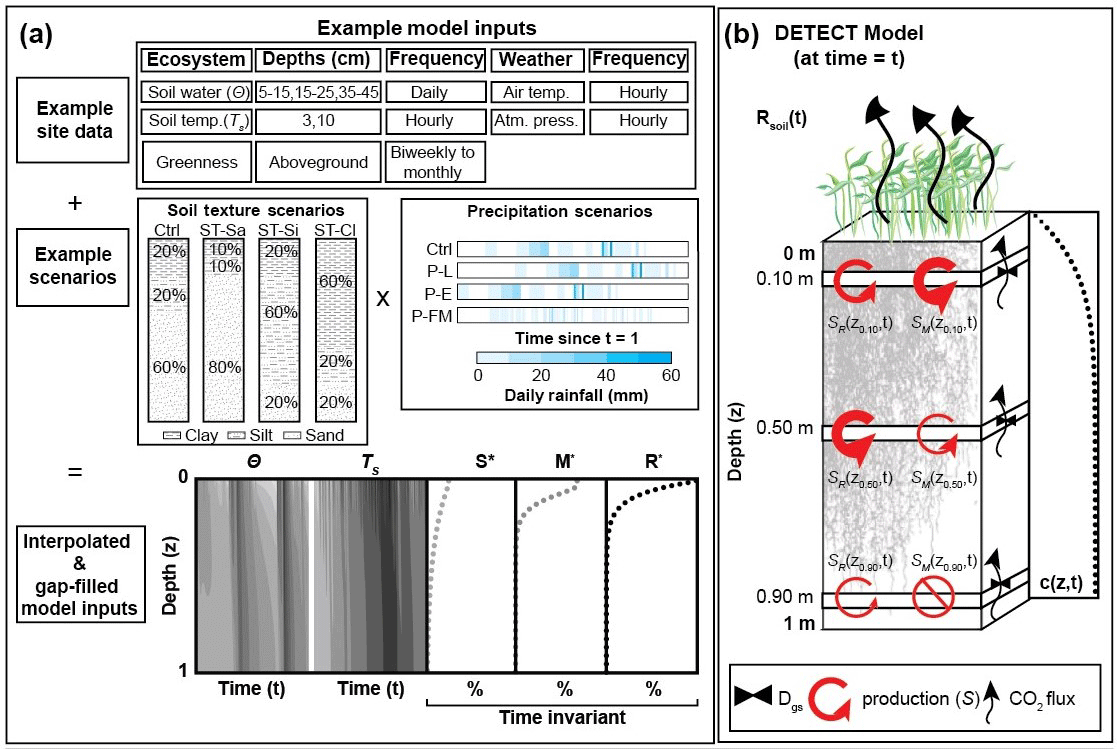
Figure 1Graphical representation of (a) the required inputs to the DETECT model and the associated scenarios implemented in this study; and (b) the components of the DETECT model at a particular time t, indicating depth-dependent production, CO2 concentrations, and CO2 fluxes.
2.1.1 Soil CO2 diffusivity submodel
The diffusivity of CO2 within the soil (Dgs) depends on the soil structure and water content; we modeled Dgs using the Moldrup function (Sala et al., 1992; Moldrup et al., 2004). We chose this formulation because it is more accurate than other common models, such as the Millington and Quirk (1961) and Penman (1940) models (Moldrup et al., 2004). Based on Moldrup et al. (2004), Dgs (m2 s−1) is defined as
where and m2 s−1 is the diffusion coefficient for CO2 in air at standard temperature (T0, 273 K) and pressure (P0, 101.325 kPa); TS(z,t) is the soil temperature (Kelvin) at depth z and time t, and P(t) is the air pressure (kPa) just above the soil surface at time t. The remaining terms in Eq. (2) include φg(z,t), the air-filled soil porosity, which is related to the total soil porosity (φT) and volumetric soil water content (θ) according to , and φT(z) is defined as , where BD and PD are the bulk density and particle density of the soil, respectively (Davidson et al., 2006); φg100(z) is the air-filled porosity at a soil water potential (Ψ) of −100 cm H2O (about −10 kPa); b(z) is a unitless parameter that is related to the pore size distribution of the soil based on the water retention curve given by , where Ψe(z) is the air-entry potential – calculated from measurements (Morgan et al., 2011) – and θsat(z) is the saturated soil water content (v∕v).
2.1.2 CO2 source (production) terms
Soil CO2 can be produced in the soil (S term in Eq. 1) by five different biological processes: (i) root growth respiration, (ii) root maintenance respiration, (iii) consumption of rhizodeposits by root-associated microorganisms and associated microbial respiration, (iv) microbial decomposition of newly produced plant litter that has been incorporated into the soil matrix, and (v) microbial decomposition of older soil organic matter (SOM) (Pendall et al., 2004). Due to the general lack of sufficient data and process understanding to accurately separate all five sources, the DETECT model treats CO2 production as the sum of two main contributions: CO2 respired by (1) roots and closely associated microorganisms (the sum of i–iii), giving SR(z,t), and (2) free-living soil microorganisms (the sum of iv–v), giving SM(z,t). Such simplification based on root and microbial sources is common in models of soil CO2 transport and production (Šimůnek and Suarez, 1993; Fang and Moncrieff, 1999; Hui and Luo, 2004). Although DETECT v1.0 assumes that root and microbial respiration are independent of one another, they both depend on the same environmental data (e.g., θ and TS).
CO2 production by root respiration is represented as the product of three terms: (i) the mass-specific base respiration rate (RRbase) at a reference soil temperature of TS=Tref and at average soil water and antecedent conditions, (ii) root mass expressed as the amount of root carbon, CR(z,t), and (iii) functions that rescale RRbase to account for the effect of soil water (θ), temperature (TS), and their antecedent counterparts. Antecedent temperature is denoted by , and for roots antecedent soil water is given by . In general, SR(z,t) is given by
The functional form of CR(z,t) is informed by field data on root biomass C (see Sect. S1 for complete details). The functions f and g are given by
, and are parameters that require numerical values (Table 1; Ryan et al., 2015), θ and TS are informed by field data, and and are computed from the field data (described below). The temperature scaling function, g (Eq. 4b) was motivated by Lloyd and Taylor (1994) and has been successfully used to describe soil and ecosystem respiration (Luo and Zhou, 2010; Cable et al., 2013; Ryan et al., 2015). Eo(z,t) is analogous to an energy of activation term that governs the apparent temperature sensitivity of SR (Davidson and Janssens, 2006; Cable et al., 2011; Tucker et al., 2013); we assume Eo responds to antecedent temperature, reflecting a potential thermal acclimation response (Atkin and Tjoelker, 2003; Ryan et al., 2015). To is also related to the apparent temperature sensitivity (Cable et al., 2011), and we assume that it is invariant with depth and time (Lloyd and Taylor, 1994; Cable et al., 2013; Barron-Gafford et al., 2014; Ryan et al., 2015). While the functional forms and choice of environmental drivers used for f and g were motivated by previous analyses (Cable et al., 2013; Barron-Gafford et al., 2014), the exact functions and parameter values were based on Ryan et al. (2015) and Cable et al. (2013). Exponential functions are also used for the moisture (f) and temperature (g) scale functions to ensure f>0 and g>0 (Eq. 4a). The choice of an exponential form of the functions was based on Ryan et al. (2015), with graphical forms of the total CO2 production based on these functions given in Fig. S10 (Supplement). However, the DETECT model is flexible enough to accommodate alternative functions for f and g. For example, we ran DETECT for the control scenario using a bell-shaped function that described how soil CO2 production changes with θ (Sect. S4 and Fig. S8, Supplement) as an alternative to Eq. (4a). For this alternative model run, the modeled Rsoil was very similar to the modeled Rsoil from the results of this study (Fig. S9, Supplement).
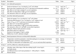
Table 1Summary of scalar parameters used in the non-steady-state (DETECT) model, arranged into four groups: parameters unique to the microbial respiration submodel for SM(z,t) (group 1); parameters unique to the root respiration submodel for SR(z,t) (group 2); parameters that are shared between the SM(z,t) and SR(z,t) submodels (group 3); parameters used to calculate soil CO2 diffusivity, Dgs (group 4). See Sect. 2.4.5 for details about how the parameters were estimated.
CO2 production by microbial respiration and SOM decomposition is represented by a modified version of the Dual Arrhenius and Michaelis–Menten (DAMM) model (Davidson et al., 2012). We exclude the O2 term, rendering the model relevant to systems that are typically unlimited by O2 availability, such as the semi-arid site that we focus on, but we accounted for a microbial C pool (CMIC) and a soluble soil-C pool (CSOL) (Todd-Brown et al., 2012) such that
Decomposition is assumed to be an enzymatic process that follows Michaelis–Menten kinetics, where Vmax is the maximum potential decomposition rate, and Km (the half-saturation constant) is the amount of substrate required for the decomposition rate to reach half of Vmax. Carbon-use efficiency (CUE) represents the proportion of total C assimilated by microbes that is allocated for microbial growth (Tucker et al., 2013). We excluded a microbial death rate term (Todd-Brown et al., 2012) because we had insufficient data on death rates, and CMIC is only ∼ 1 % of CSOL at our study site (Carrillo and Pendall, 2018).
In contrast to the original DAMM formulation, we allowed SM(z,t) and to vary by depth and time, whereas existing applications of the DAMM model are generally applied to “bulk” soil (i.e., do not vary with z). We also modeled Vmax according to the modified energy of activation function described in Lloyd and Taylor (1994), which essentially parallels Eq. (4b)–(4c):
VBase is the “base” Vmax at a reference soil temperature of Tref and at mean values of current θ and antecedent θ and TS (i.e., mean values of and . Eo(z,t) and follow the same functional forms and interpretation as described for the root respiration submodel (Eqs. 3 and 4a–c), except that is used instead of , respectively, and different values are specified for the parameters α1, α2, α3, α4, To, and to reflect microbial respiration The values are given in Table 1, and Sect. 2.4.5 explains how the values were estimated.
Finally, CSOL is modeled as a function of soil organic C content at depth z, CSOM(z) based on the fraction, p, of CSOM(z) that is soluble and the diffusivity of the substrate in liquid, Dliq (Davidson et al., 2012). The equation for CSOL is given by
The values of p and Dliq were taken from laboratory analysis (see Sect. 2.4.5) and Davidson et al. (2012), respectively. We assumed that CSOM(z) and CMIC(z) (see Eq. 5) are constant over time given the relatively short simulation periods explored here (a single growing season); but the model could easily be modified to allow for time-varying CSOM and CMIC. Here, CSOM(z) and CMIC(z) are simple, empirical functions that were informed by data (see Sect. S1 for details). Moreover, while assumption of time invariant CSOM(z) and CMIC(z) is an implicit SS assumption about biological factors affecting soil CO2 dynamics, this assumption allows us to isolate the importance of NSS conditions that are primarily due to physical CO2 transport characteristics.
2.1.3 Soil respiration
The efflux of CO2 from the soil surface (soil respiration, Rsoil) is computed as
is the diffusivity of CO2 in the soil and is the total CO2 concentration (microbial- and root-derived), respectively, at z=0.01 m depth and time t; catm(t) is the CO2 concentration in the atmosphere above the soil surface; and Δz is the depth increment that the model solves for soil CO2 concentration (here, Δz=0.01 m).
2.2 Numerical implementation of the DETECT model
The numerical solution to the NSS version of the DETECT model v1.0, as described in Eqs. (1)–(8), requires an initial condition (IC) and two boundary conditions (BCs), which we specified as
The function c0(z) is determined and parameterized in two stages: (1) observed soil CO2 concentration data at three depths from the start of the 2007 growing season were used to parametrize a simple function that described the change in CO2 concentration for all depths; (2) the DETECT model was run forward for the growing season of 2007, then the modeled CO2 concentrations for all depths on the final day of the 2007 growing season (31 September 2007) was used as the initial condition for running the DETECT model for 2008. See Sect. S2 in the Supplement for specific details. We set catm(t) equivalent to 356 ppm for all t, which was the average near-surface, ambient atmospheric CO2 concentration measured at the PHACE site in the 2008 growing season. Following the methods of Haberman (1998), we adopted a zero-flux lower BC (Eq. 9c) due to the lack of data at or near a depth of 1 m.
Prior to solving the non-linear PDE (Eq. 1), we expanded the RHS of Eq. (1) using the “product rule for differentiation”. We then numerically solved the non-linear PDE (Eq. 1) by employing a forward Euler discretization with a centered difference method for the depth derivative at a depth increment of Δz=0.01 m. To ensure numerical stability, we calculate model outputs at a numerical time step of , where dt is the time step at which the predicted outputs are stored (6 h), and Ndt is the number of numerical time steps. Ndt is computed based on the fastest (largest) diffusion coefficient at each time step such that , where max(Dgs) is the maximum Dgs across all depth increments at time t (Haberman, 1998). We solved Eq. (1) separately for both root- and microbial-derived CO2 concentrations, such that for K=R or M:
We rearranged Eq. (10) to solve for , which was iterated forward for all time steps and depth increments; total CO2 concentration at each time step and depth is calculated as . For clarity, we emphasize that Eq. (10) is the discretized version of Eq. (1), which we require in order to numerically solve Eq. (1) (Haberman, 1998). We programmed the DETECT model v.10 and the numerical solution method in Matlab (Mathworks, 2016).
2.3 Steady-state (SS) solution to the DETECT model
A primary goal of this work was to test if soil CO2 and associated Rsoil predicted from the non-steady-state (NSS) model (DETECT) could be distinguished from that of the steady-state (SS) solution. The SS version of Eq. (1), which we refer to as the SS-DETECT model, can be solved analytically as an ordinary differential equation (ODE) by setting the term to zero (Amundson et al., 1998). As with the NSS model, we found the SS solution to Eq. (1) separately for root- and microbial-derived CO2 concentrations, and , respectively. Using the upper and lower boundary conditions described for the NSS model (Eq. 9b and c), the analytical SS solutions at time t and depth z are derived by Amundson et al. (1998) and Cerling (1984). The solution is given by
where K=R and K=M refers to the soil CO2 from root (R) and microbial (M) sources, respectively. is the depth-averaged source term for microbial or root production (averaging over 100 different 0.01 m increments). The soil CO2 diffusivity term, Dgs(z,t), and upper boundary condition, catm(t), are the same as previously defined (Eqs. 2 and 9b, respectively; Amundson et al., 1998).
2.4 Application of the DETECT and SS-DETECT models to the PHACE site
In this subsection, we provide an overview of the study site, including the PHACE experiment, and relevant data sources from PHACE that we used to drive the DETECT and SS-DETECT models. We also summarize how we calibrated the models in the context of the PHACE site, and we highlight data that we used to informally validate the general behavior of the models. We conclude by describing the simulation experiments that we conducted to test the effects of soil texture and precipitation variability on the importance of NSS versus SS soil CO2 conditions.
2.4.1 Field site and PHACE experiment
The Prairie Heating and CO2 Enrichment (PHACE) field experiment is located in south-central Wyoming (latitude N, longitude W, elevation 1930 m). The site is a mixed-grass prairie with a semi-arid climate characterized by long winters (mean January temperature = −2.5 ∘C) and warm summers (mean July temperature = 17.5 ∘C), with mean annual precipitation of 384 mm (Morgan et al., 2011). The vegetation is predominantly composed of two C3 grasses, western wheatgrass (Pascopyrum smithii (Rydb.) A. Löve) and needle-and-thread grass (Hesperostipa comata (Trin. & Rupr.)), and a C4 perennial grass, blue grama (Bouteloua gracilis (H.B.K.) Lag). The soil is a fine-loamy, mixed, mesic Aridic Argiustoll, and biological crusts are not present (Bachman et al., 2010).
2.4.2 Environmental driving data
We simulated the transport and production of soil CO2 for each 0.01 m depth increment, from the surface (0 m) to a depth of 1 m, across all 732 time steps (i.e., four time steps per day [every 6 h] for 183 days from April to September). To do this, we required soil environmental data consisting of water content (θ) and temperature (TS) and meteorological data including precipitation, air temperature, and air pressure. The θ and TS data that were used to drive the DETECT model were created using the HYDRUS software (see Sect. 2.4.3), calibrated against actual measurements of θ and TS. For the meteorological data, actual measurements from the PHACE site were used.
The PHACE experiment involved an incomplete factorial of CO2, warming, and irrigation (six treatment levels total), with five replicate plots per treatment level, resulting in a total of 30 instrumented plots. One of the five plots from the control treatment – ambient CO2, temperature (no heating), and precipitation (no supplemental irrigation) – was chosen at random and had a system installed to measure soil CO2 concentrations continuously for three different soil depths (3, 10, and 20 cm). This plot, therefore, provided the data for driving the DETECT and SS-DETECT models. Data that we used were collected during the growing season (March–September) of 2008; θ was measured hourly at three depths (5–15, 15–25, and 35–45 cm; EnvironSMART probe, Sentek Sensor Technologies, Stepney, Australia) and we used daily averages to drive the models. TS was measured hourly at two depths (3 and 10 cm) using type-T thermocouples. Hourly precipitation (mm), air temperature (∘C), relative humidity (%), and surface barometric air pressure (kPa) were recorded by an automated weather station at the site.
2.4.3 High-resolution environmental data
To accommodate the 0.01 m depth increments specified for the DETECT model, we used the coarse-resolution field data (above) to create finer-resolution driving data. For example, temporal gap-filling of the θ,TS, and micrometeorological datasets was required due to gaps that occurred during a small number of days (< 1, 6, and 2.5 %, respectively) as a result of instrument failure. We used data from other nearby plots to estimate the values of the missing data, but we also used cubic spline interpolation where gaps remained. Details of these gap-filing methods can be found in Ryan et al. (2015).
We used HYDRUS-1D v4.16.0090 to simulate θ and TS in 0.01 m increments from a depth of 0.01 to 1 m (Chou et al., 2008; Šimůnek et al., 2008; Piao et al., 2009) based on precipitation data at the site. HYDRUS simulates the movement of water by solving the Richards' equation for water movement (Richards, 1931; Chou et al., 2008; Sitch et al., 2008) and heat transport via Fickian based advection–dispersion equations. Soil hydraulic and heat transport parameters were estimated in HYDRUS using the inverse mode to solve for parameter values based on the PHACE θ (5–10, 15–25, and 35–45 cm) and TS (3 and 10 cm) data (Šimůnek et al., 2005, 2008). HYDRUS was then run in forward mode based on the tuned soil hydraulic parameters to estimate θ and TS at all 100 different 0.01 m depth increments at six-hourly time intervals. For consistency, HYDRUS-derived θ and TS were used as the environmental input data to the DETECT models, even at the depths for which PHACE data were available.
2.4.4 Antecedent soil water and soil temperature conditions
We explicitly evaluated the impact of antecedent (past) θ and TS conditions on CO2 production by roots and microbes, motivated by prior work that estimated the relative importance of antecedent conditions and their time scales of influence on soil and ecosystem CO2 efflux (Cable et al., 2013; Barron-Gafford et al., 2014; Ogle et al., 2015; Ryan et al., 2015). Antecedent soil water content and antecedent soil temperature – and , respectively, for K=R (roots) and M (microbes) were computed as weighted averages of the HYDRUS-produced θ(z,t) and TS(z,t) data, respectively. These calculations were done external to the DETECT model, and the antecedent variables were supplied as driving variables to DETECT. For example, for each 0.01 m increment (z) and time period (t), antecedent soil water associated with microbial CO2 production was calculated as
The w's are the antecedent importance weights, which sum to 1 from j=1 (previous time period) to j=J (J previous time periods). The weights were informed by results from an analysis of ecosystem respiration at the PHACE site (Ryan et al., 2015). For microbes, J=4 days and w=(0.75, 0.25, 0, 0), indicating the strong importance of θ conditions occurring the previous day (j=1) (Oikawa et al., 2014). Similar equations were used to compute and , each with their own set of weights (w's) and time scales (J's). For example, the time step and J for θ differ among microbes (2 days) and roots (3 weeks); for roots, was computed as a weighted average of past, average weekly values of θ, with j denoting weeks into the past, for J=4 weeks, and w=(0.2, 0.6, 0.2, 0), indicating a strong lag response to θ conditions occurring two weeks ago (Cable et al., 2013; Ryan et al., 2015). For antecedent soil temperature, we assumed that each of the past four days were equally important by setting the w vectors to (0.25, 0.25, 0.25, 0.25), for both microbes and roots (Ryan et al., 2015). The specification of J and the w's are independent of the DETECT model formulation and can be varied by the user. For clarity we summarize these weight parameters in Table 2.
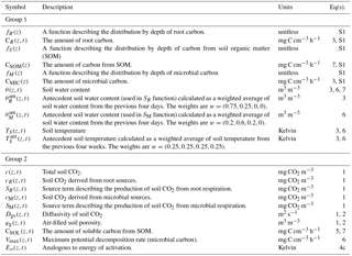
Table 2Summary of quantities in the non-steady-state (DETECT) model that vary by depth only (z), or by depth (z) and time (t). Those in group 1 represent input variables (derived prior to the running of the DETECT model), while group 2 contains the modeled quantities (used as part of the operation of the DETECT model). Equation (S1) can be found in Sect. S1 in the Supplement.
2.4.5 Overview of parameterization approach using PHACE data
In general, our aim was to specify realistic values for the parameters in the DETECT model. We did not formally “fit” the DETECT model to data, but rather, we simply determined reasonable values based on simple analyses of relevant PHACE data sets, results published for the PHACE site, or results from other relevant studies. The full list of parameters is given in Table 1, and below we describe the logic behind specifying the values in Table 1.
The depth-distributions of root biomass C (CR, Eq. 3), soil microbial biomass C (CMIC, Eq. 5), and soil organic C (CSOM, Eq. 7) are expressed in terms of a total C content in a 1 m deep soil column (R*, M*, and S*, respectively; mg C cm−2), multiplied by the proportion of that C that occurs at depth z (fR(z), fM(z), and fS(z), respectively). See Sect. S1 (Supplement) for details. Regarding the data, soil organic C (Fig. S5, Supplement) was determined by combustion of acidified, root-free soil collected from 0–5, 5–15, 15–30, 30–45, 45–75, and 75–100 cm depths, using a Costech Elemental Analyzer. Microbial biomass C was determined by the chloroform fumigation and extraction in 0.05 M K2SO4 (Carrillo et al., 2014b). Extracts were analyzed for total C on a total organic carbon analyzer (Shimadzu TOC-VCPN; Shimadzu Scientific Instruments, Wood Dale, IL, USA) after treating with 1 M H3PO4 (1 µL per 10 mL of extract) to remove any carbonates. Root biomass C was estimated from ash-free root biomass and elemental analysis (Carrillo et al., 2014a; Mueller et al., 2016). The solubility parameter, p, was estimated as the ratio of CSOL to CSOM using measurements of these two quantities which were based on unfumigated extracts obtained for microbial biomass estimations as above (CSOL) and on total C concentration in soil (CSOM).
The values used for the base microbial respiration rates and the half-saturation constant (VBase [Eq. 6] and Km [Eq. 5]; Table 1) were estimated by fitting the microbial respiration submodel, but without the CMIC or CUE terms (Eq. 5), to microbial respiration data from the PHACE control plots (Fig. S7, Supplement). The CMIC and CUE terms were not included in this earlier version of SM submodel – which was used for model calibration purposes – because we did not have measurements of these two variables at the time. We estimated VBase and Km using a Markov chain Monte Carlo approach, identical to the approach used in Ryan et al. (2015). In the absence of root respiration data, we assumed that base root respiration (RRbase [Eq. 3]; Table 1) was proportional to the microbial base rate term (Hanson et al., 2000). The parameters denoting the effects of current soil moisture (e.g., α1; Eq. 4a), antecedent moisture (α2), and the interaction between current and antecedent moisture (α3) on root and microbial respiration were derived from Ryan et al. (2015), based on an analysis of ecosystem respiration (Reco) data from PHACE. However, we adjusted the values (Table 1) by trial and error to reflect the expectation that the effects of current soil moisture should be stronger for microbial compared to root respiration because microbes tend to respond more rapidly to precipitation pulses (Risk et al., 2008), whereas root respiration is likely to show a delayed response which depends more strongly on past moisture conditions (Cable et al., 2008, 2013). Of the remaining two parameters describing SM (Eqs. 5–6; Table 1), the value of CUE was based on results from a soil incubation study conducted at a nearby site (Tucker et al., 2013), whilst our value for Dliq was taken from Davidson et al. (2012). Three parameters (, To, and α4; Eq. 4a–b) were shared between the SR and SM submodels, and their values were also obtained from Ryan et al. (2015). Finally, the parameters used for CO2 diffusivity (b, BD, and φg100; Eq. 2) were based on published, site-specific data (Morgan et al., 2011).
2.4.6 Informal model validation with soil respiration measurements
We evaluated the accuracy of the DETECT model by comparing (1) predicted Rsoil (Eq. 8) against plot-level measurements of ecosystem respiration (Reco) (see below) and (2) predicted soil CO2 concentrations, c(z,t), versus observed concentrations; all observed data were from the PHACE study. Since we did not rigorously parameterize the DETECT model with PHACE data, we were simply looking for reasonable, qualitative agreement between the modeled variables and the observations (e.g., similar order of magnitude, comparable temporal trends). Observed Reco was measured on control plots every two to four weeks during the target growing season, using a canopy gas exchange chamber, and instantaneous fluxes were scaled to daily rates using a linear, empirical function (Jasoni et al., 2005; Bachman et al., 2010). We assumed that Rsoil was similar to Reco given that aboveground biomass was < 20 % of total plant biomass (Mueller et al., 2016). Measurements of microbial respiration were obtained by applying glyphosate herbicide to small subplots in May 2008, limiting ecosystem CO2 efflux to microbial sources (Pendall et al., 2013), Non-steady state soil chambers were used to estimate the resulting surface soil fluxes every two weeks around midday (Oleson et al., 2013; Ogle et al., 2016). Soil CO2 concentrations were also measured with non-dispersive infrared sensors (Vaisala GM222, Finland) installed at 3, 10, and 20 cm below the soil surface, averaged on an hourly basis (Risk et al., 2008; Vargas et al., 2011; Brennan, 2013). Observations of soil [CO2] for control plots were compared against predictions of c(z,t) at z=0.03, 0.1, and 0.2 m and at the corresponding times.
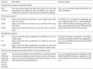
Table 3The scenario code, description, and summary of results associated with each model scenario; the 14 scenarios below were applied to both the DETECT and SS-DETECT models. The scenarios involved a non-factorial combination of different soil texture, precipitation regimes, and inclusion/exclusion of antecedent effects on the root and microbial CO2 production rates.
2.5 Simulation experiments
We evaluated the impact of three potentially important factors that could affect the frequency of NSS (Eqs. 1 and 9a–c) relative to SS (Eq. 11) conditions: (1) soil texture, (2) precipitation patterns, and (3) importance of antecedent conditions. In the control (Ctrl) scenario, we calculated the source terms and diffusion terms (SK and Dgs in Eqs. 1 and 2) based on soil environmental (θ and TS), soil texture (sandy clay loam: 60 % sand, 20 % silt, 20 % clay), and meteorological data (e.g., precipitation) measured at the PHACE site in 2008. We varied soil texture, relative to that of the site, by altering the relative amounts of sand, silt, and clay, giving three levels (Table 3): 80 % sand, 10 % silt, and 10 % clay (sandy loam, scenario denoted as ST-Sa); 20 % sand, 60 % silt, and 20 % clay (silt loam, ST-Si); 20 % sand, 20 % silt, and 60 % clay (clay, ST-Cl). The control (Ctrl) scenario was also paired with the observed daily precipitation data for 2008. We explored three additional precipitation scenarios, under the control soil texture, by shifting the daily precipitation to occur one month earlier, or one month later, or by using precipitation data from 2009 (scenarios P-E, P-L and P-FM, respectively; Table 3). For P-FM, we chose 2009 because it had approximately the same total precipitation between April and September as 2008 (340 and 348 mm for 2008 and 2009, respectively), but it fell as more frequent events of smaller magnitudes. For each texture and precipitation scenario, HYDRUS was used to compute the corresponding TS and θ at the required depth and time intervals. Specifically, the different soil texture and precipitation regimes were used as inputs for the HYDRUS software when generating TS and θ for all 100 depths and all 732 time points. Hence, the differences in soil texture and differences in precipitation regimes were implemented by using different input files for the HYDRUS-generated θ and TS data.
All of the above scenarios assumed that antecedent conditions were not important, which was achieved by setting all antecedent effects parameters (α2, α3, and α4; Table 1) equal to zero. We contrasted these scenarios against ones that included antecedent conditions (thus, computed and in Eqs. 3 and 6) in the calculation of soil CO2 production by roots (K=R) and microbes (K=M); all such scenario names were appended with “ant” (Table 3, Fig. 1a). For each scenario summarized in Table 3, we evaluated the potential for NSS conditions by comparing the predicted Rsoil produced by the DETECT model versus the SS-DETECT model.
3.1 Control scenarios
Soil CO2 was in steady state (SS) during most of the growing season under the control soil texture (sandy clay loam) and precipitation conditions that assumed no antecedent affects (Ctrl scenario). For example, soil respiration (Rsoil) predicted by the DETECT model was approximately equal to Rsoil predicted by the SS-DETECT model during times of no or little precipitation (Fig. 2a, days < 218 or > 230). Conversely, Rsoil predicted by the SS-DETECT model was temporarily greater and more variable than that predicted by the DETECT model immediately following a large precipitation event (Fig. 2a, days 218–229). However, the total cumulative Rsoil between days 92 to 274 – hereafter “total growing season Rsoil” – under SS (497 g C m−2) versus NSS (498 g C m−2) assumptions was approximately equal (a difference of ∼ 0.2 %).
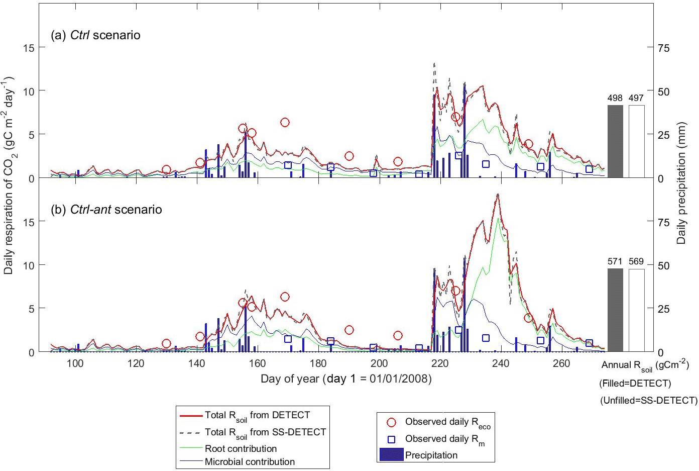
Figure 2Time series of daily surface soil CO2 fluxes (Rsoil) predicted by the non-steady-state (DETECT) and steady-state (SS-DETECT) models over the growing season (1 April–30 September), based on the control scenarios (a) without (Ctrl) and (b) with (Ctrl-ant) antecedent effects (see Table 2). Only Rsoil is simulated using the SS-DETECT model, whereas Rsoil and its root and microbial contributions are simulated using the DETECT model. The predicted fluxes are overlaid with observed ecosystem respiration (Reco; Rsoil+ aboveground plant respiration) and microbial respiration (Rm; based on plots where vegetation was removed).
The differences between the Rsoil from DETECT and SS-DETECT using the antecedent parametrization of the source terms of the models (Ctrl-ant scenario; Fig. 2b) were generally consistent with the results from the Ctrl scenario (Fig. 2a). However, the magnitude of Rsoil predicted by both the DETECT and SS-DETECT models was up to 9 g C m−2 day−1 greater during days following the major rain event (i.e., during days 230–243) when antecedent conditions were considered. Moreover, the incorporation of antecedent effects led to a longer delay between the timing of the major rain event and the maximum Rsoil, which occurred ∼ five days later than when only current conditions were considered (Fig. 2a vs. 2b). As a result, total growing season Rsoil was ∼ 15 % higher under the Ctrl-ant scenario (e.g., 571 g C m−2 under NSS assumptions, Fig. 2b) compared to the Ctrl scenario (e.g., 498 g C m−2 under NSS, Fig. 2a). This increase in predicted Rsoil under the Ctrl-ant scenario for days 230–243 was primarily driven by greater root respiration (Fig. 2a vs. 2b).
3.2 Effects of soil texture
Varying soil texture resulted in the greatest difference in daily Rsoil between the DETECT and SS-DETECT models; however, integrated over the growing season, these differences were very small (Fig. 3a, b, c). In particular, total growing season Rsoil predicted by SS-DETECT was ∼ 1.5 % less than predicted by DETECT for soils consisting primarily of sand and silt (ST-Sa and ST-Si scenarios; Fig. 3a, b), but was ∼ 3.3 % less for a clay dominated soil (ST-Cl scenario; Fig. 3c red versus grey bars). These differences in Rsoil under NSS versus SS assumptions were approximately the same for the scenarios involving antecedent effects (Fig. 3d, e, f). Despite the minor differences at the growing season scale, notable differences emerged at the daily scale. For example, with the largest precipitation event of the year and the 10 days that followed (days 218–228), the median absolute difference between daily Rsoil from the SS-DETECT and DETECT models was 22–24 % for the ST-Sa and ST-Si scenarios regardless of whether or not antecedent variables are included (Figs. 3 and S3a, b). These differences increased to 31–35 % for the two clay soil texture scenarios (ST-Cl and ST-Cl-ant).
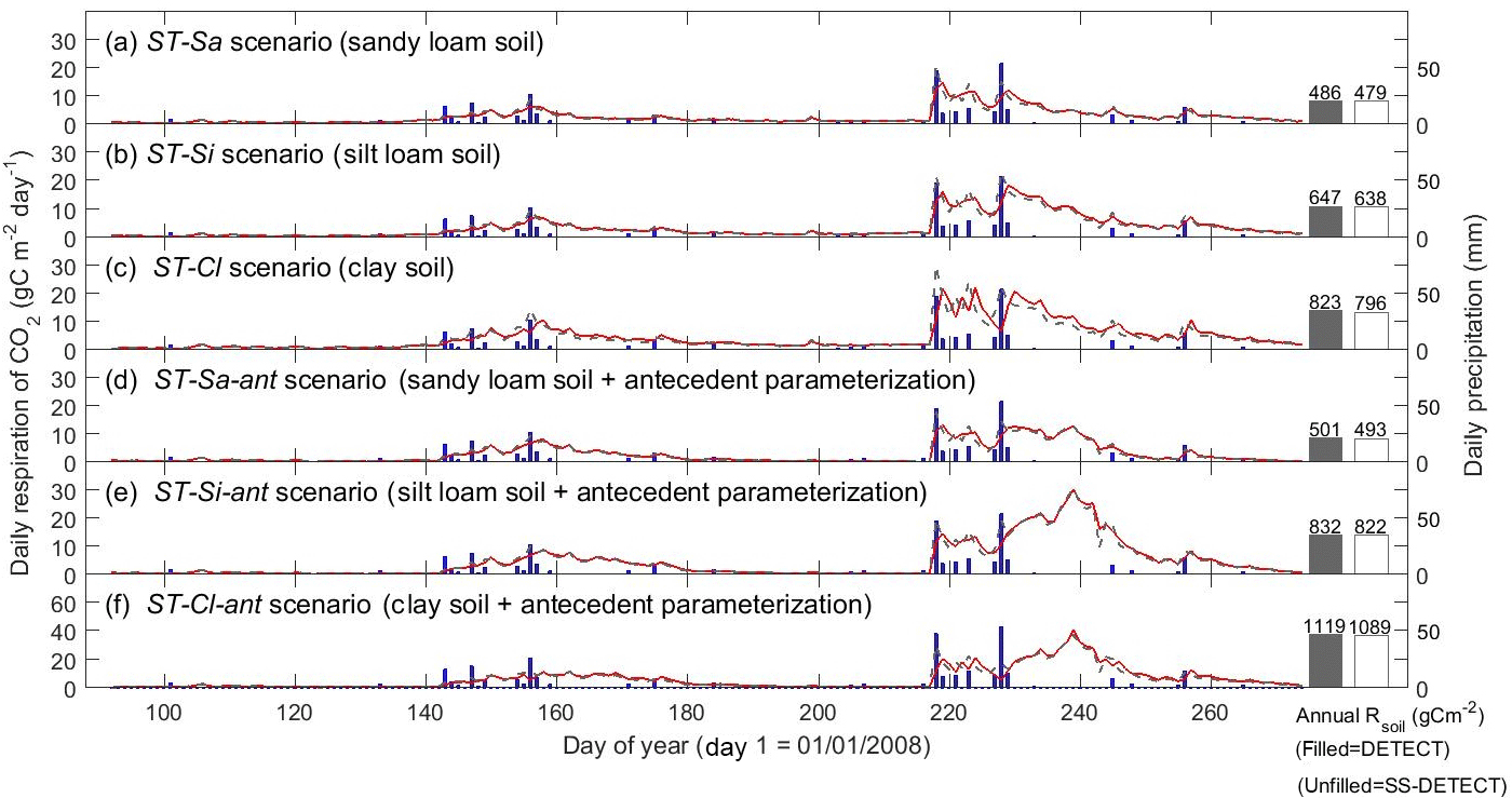
Figure 3Time series of daily surface soil respiration (Rsoil) predicted from the non-steady-state (NSS) DETECT model (red solid lines) and the steady-state (SS-DETECT) model (grey dashed lines), for different soil texture scenarios. The first three scenarios are the same as the control (Ctrl), except they assume a different soil texture: (a) more sandy soil, (b) more silty soil, or (c) more clayey soil. Panels (d), (e), and (f) show the Rsoil predictions from the same soil texture scenarios as in (a)–(c), but also include the antecedent effects of soil moisture and temperature. See Table 2 for descriptions of each scenario. Rsoil predictions are overlaid with daily precipitation.
Soil texture also affected the magnitude of predicted Rsoil compared to the control scenarios, both with and without antecedent effects (Ctrl-ant and Ctrl, respectively). In particular, we found that total growing season Rsoil, whether from the DETECT or the SS-DETECT model, was ∼ 30 % and ∼ 60 % higher for the ST-Si and ST-Cl scenarios relative to the Ctrl scenario (Figs. 3b, c, 4a). The change in Rsoil was negligible, however, when the sand content was increased from 60 % (Ctrl) to 80 % (ST-Sa) for both models (Figs. 3a, 4a). The antecedent versions of the fine-textured scenarios (ST-Si-ant and ST-Cl-ant) resulted in ∼ 45 and ∼ 95 % increases in total growing season Rsoil, respectively, compared to the Ctrl-ant scenario (Figs. 3e, f, 4b). As with the Ctrl-ant scenario (Sect. 3.1), greater root respiration following the end of the second precipitation period between days 230 and 245, primarily drove the larger percentage increases for the SL-Si-ant and SL-Cl-ant scenarios compared to the non-antecedent versions.
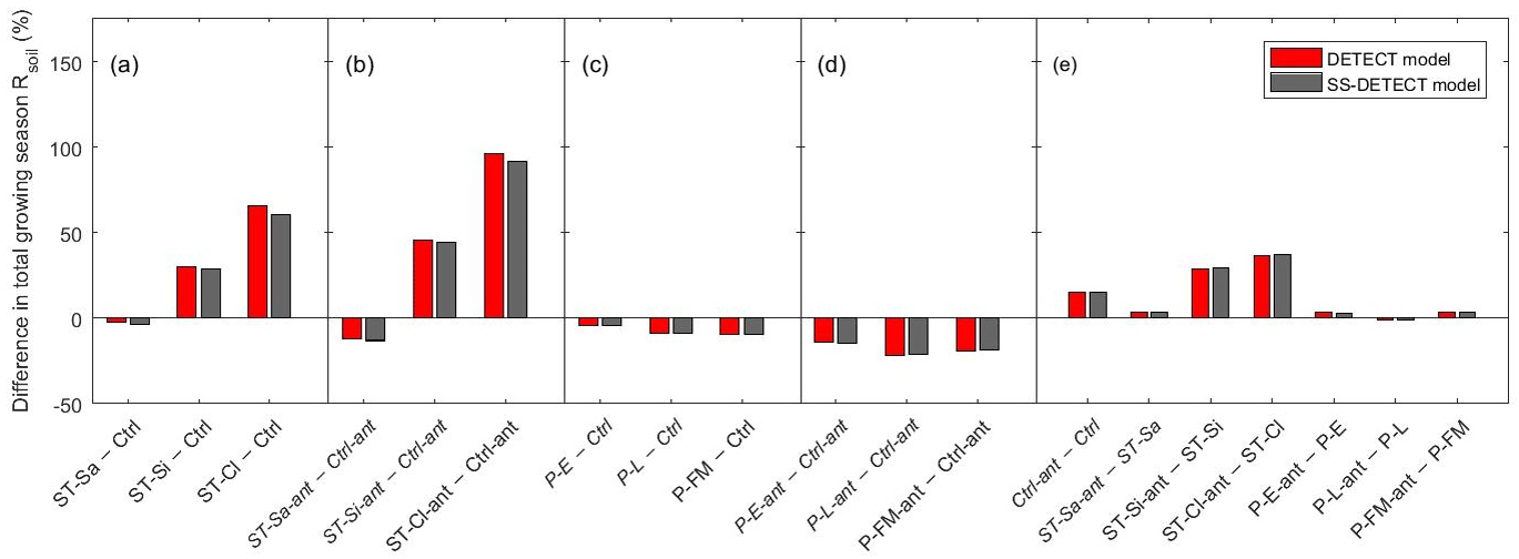
Figure 4Differences of total growing season (April–September) soil respiration (Rsoil) as predicted by the non-steady-state (DETECT) and steady-state (SS-DETECT) models, for different pairs of scenarios. Comparisons are grouped so that they quantify the effects of (a) soil texture without antecedent effects, (b) soil texture with antecedent effects, (c) precipitation without antecedent effects, (d) precipitation with antecedent effects, and (e) antecedent effects. See Table 2 for descriptions of each scenario.
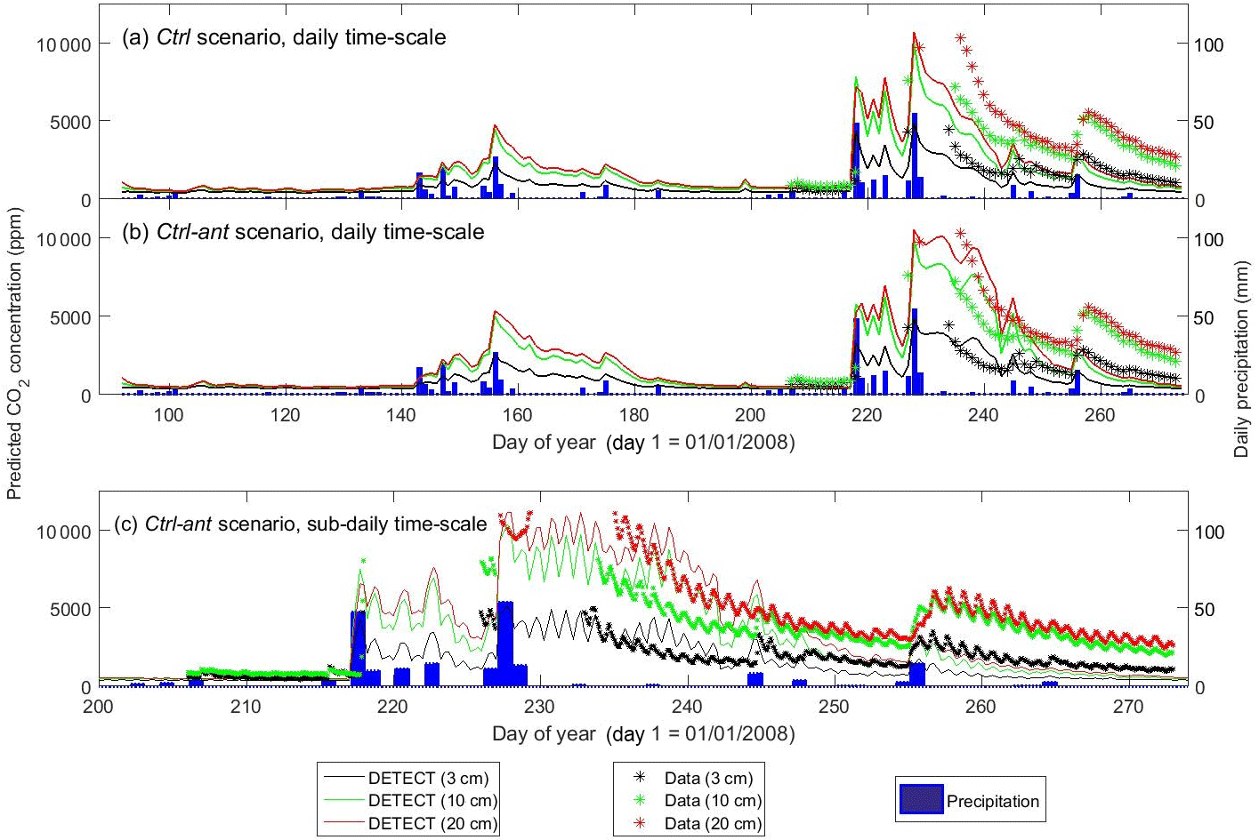
Figure 5Time series of predicted versus observed soil CO2 concentrations at 3 cm depth, 10 cm depth, and 20 cm depth, where the predictions are based on the non-steady-state (NSS) DETECT model. Predicted [CO2] is shown for the daily time scale for the control scenarios (a) without (Ctrl) and (b) with (Ctrl-ant) antecedent effects, and for (c) the subdaily (every 6 h) time scale for the Ctrl-ant scenario. Units are in parts per million (ppm).
3.3 Effects of precipitation regimes
Although varying the timing, frequency, or magnitude of precipitation led to little difference between Rsoil as predicted by the DETECT and SS-DETECT models (Fig. S2), these precipitation regimes did affect the magnitude of Rsoil predicted by both models. For example, total growing season Rsoil predicted under the alternative precipitation scenarios was lower relative to the Ctrl scenario. This decrease was relatively small (5–10 %) for the non-antecedent versions of the models (Fig. 4c), but was comparatively larger (15–22 %) for the antecedent versions (Fig. 4d). This reduction appears to be driven by the amount of time over which daily Rsoil responded to the second precipitation period, which occurred around day 220, 190, and 250 in the Ctrl, P-E, and P-L scenarios, respectively. Following this precipitation event, daily Rsoil achieved values around 10 g C m−2 day−1 for about 20 days in the Ctrl scenario (Fig. 2a, days 220–240), but for only about five days in the P-E and P-L scenarios (Fig. S2a, b, after days 190 and 250, respectively). Increasing the frequency of precipitation while retaining approximately the same annual amount (i.e., scenario P-FM) resulted in daily Rsoil being consistently less than that of the Ctrl scenario, which led to a reduction in total growing season Rsoil in the P-FM scenario (Fig. S2c).
3.4 Effects of antecedent responses
When antecedent soil water content and soil temperature were included in the DETECT model we found that predicted Rsoil was 15 % greater for the control scenario and 29–37 % greater for the fine textured soil scenarios, compared to the corresponding scenarios that did not include antecedent conditions (Fig. 4e). When the sand content was 80 % or for any of the different precipitation regimes, there was a negligible difference between Rsoil predicted by the antecedent versus non-antecedent parametrizations of DETECT.
Daily Rsoil predicted by the DETECT model based on the Ctrl and Ctrl-ant scenarios agreed well with observed ecosystem respiration (Reco), but Reco was slightly higher than predicted Rsoil (Fig. 2a, b), which was expected since aboveground autotrophic respiration. For the most part, this data-model agreement was similar whether the antecedent model terms were included (Fig. 2b) or not (Fig. 2a). Unfortunately, Reco data were not available during the time period (days 230–250) associated with the greatest disagreement between the Ctrl and Ctrl-ant scenarios. During this period, frequent hourly measurements of soil [CO2] were in better agreement with predicted soil CO2 from the Ctrl-ant scenario compared to the Ctrl scenario (Figs. 5a, b, S4a, b). After day ∼ 250, based on the DETECT model, both scenarios (Ctrl and Ctrl-ant) under-predicted the observed soil [CO2] by ∼ 50 % (Fig. 5).
The DETECT and SS-DETECT models provide a framework for evaluating the circumstances under which steady-state (SS) assumptions of soil CO2 production and surface soil respiration (Rsoil) are valid, and to identify the major physical (i.e., soil texture, soil moisture) and/or biological (i.e., root and microbial respiration responses) factors that lead to non-steady-state (NSS) conditions.
4.1 Steady-state versus non-steady-state conditions
At the seasonal scale, there was reasonable agreement between total growing season Rsoil predicted under the assumption of SS versus NSS conditions, but the strength of this agreement depended on soil texture (see Sect. 4.2). At the daily scale, Rsoil predicted by the DETECT model deviated from values expected under the assumption of SS conditions for 11 days or 4 % of the days during the April-September growing season (Fig. 2, days 218–228). These discrepancies, attributed to NSS conditions, were generally limited to periods following large rain events. For applications that assume SS conditions, such as isotopic partitioning studies (Hui and Luo, 2004; Ogle and Pendall, 2015), the SS assumption seemed reasonable during periods of minimal or no precipitation, representative of times during which soil water content changes very little or gradually. For sites or time periods characterized by pulsed precipitation patterns, our results suggested that NSS conditions would be more likely over longer periods of time.
4.2 Effect of varying soil texture
Our results indicated that soil texture exerts the strongest control over the prevalence of NSS soil CO2 conditions. For a predominantly (e.g., 60 %) sandy or silty soil, soil CO2 transport and efflux generally aligned with the SS assumption (Figs. 2, 3a–b). This was consistent with previous work that used SS models to predict Rsoil for similar soil types (Baldocchi et al., 2006; Vargas et al., 2010).
For very fine-texture soil dominated by clay, however, SS assumptions were far less appropriate. The larger difference – relative to the Ctrl scenario – in Rsoil predicted under SS versus NSS conditions for fine-texture (i.e., 60 % clay) soil was apparent at both the growing season scale and the daily scale following a large precipitation event (Figs. 3, S3a, b). In general, the DETECT model predicted that Rsoil should be higher in clay compared to sandy soil after precipitation events, a result supported by field experiments (Cable et al., 2008), but this texture effect is muted under assumptions of SS. Moreover, recovery of Rsoil to SS rates after a large rain event took ∼ 30 days in the clay soil (Fig. 3c, days 218 to 248) compared to ∼ 10 days for the other coarser soil texture scenarios (Figs. 2, 3a–b, days 218 to ∼ 230). These effects of soil texture on the prevalence of NSS conditions can be attributed to soil physical properties and their effects on air-filled porosity and CO2 diffusivity. Fine textured soils have smaller pores and tend to retain water for longer (Bouma and Bryla, 2000), which has the effect of decreasing soil CO2 diffusivity (Fig. 6). Thus, under moist conditions that follow a rain event, it may take about 15 min for a CO2 molecule produced at 0.5 m to diffuse to the surface in a clay soil compared to only 1–2 min for a sandy soil. This means that the increase in CO2 concentration near the soil's surface will be almost immediate under a coarsely textured soil (Fig. 6a), but slightly delayed under a finely texture soil. Finally, fine-textured soils have slower infiltration rates (Hillel, 1998), delaying the exposure of more deeply distributed roots and microbes to increased moisture availability. While this effect may not directly impact the SS assumption, it would lead to greater time lags between precipitation pulses and Rsoil peaks.
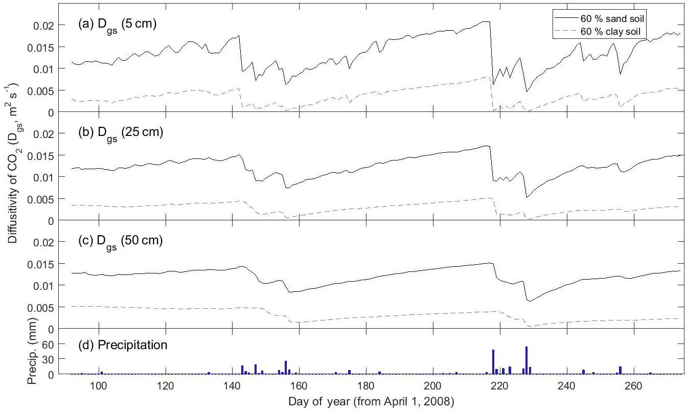
Figure 6Time series of how the modeled diffusivity of CO2 (Dgs) at three different depths (5, 25, and 50 cm) varies between a predominantly sandy soil (solid line) and a predominantly clay soil (dashed line). Predictions are from the non-steady state (DETECT) model for the Ctrl (60 % sand) and ST-Cl (60 % clay) scenarios; see Table 2 for a description of the scenarios.
These findings have important implications for studies that rely on the SS assumption to predict subsurface soil CO2 production. The SS assumption may be sufficient for systems defined by coarse-textured soils, but it may lead to erroneous conclusions if applied to fine-textured soils, especially at the very short-term scale (e.g., diurnal Rsoil) during times of precipitation. Our simulation experiments made the simplifying assumption that soil texture is constant with depth, but in many ecosystems, texture may vary greatly with depth (Ogle et al., 2004). An important next step is to extend the simulations to explore the impacts of depth-varying soil texture on SS versus NSS conditions. The DETECT model can easily accommodate such modifications; allowing soil texture to vary by depth would have a direct effect on soil water content, which is simulated outside of DETECT using HYDRUS (Chou et al., 2008; Šimůnek et al., 2008; Piao et al., 2009), and can accommodate such depth variation.
4.3 Effect of varying the timing or frequency of precipitation
Unlike soil texture, varying the timing, frequency, and magnitude of precipitation resulted in predicted Rsoil that was almost identical under SS and NSS assumptions, both at the growing season and daily time scales (Fig. S2). We had anticipated that such changes in the precipitation regime would impact SS conditions via impacts on soil air-filled porosity and potentially by changing the covariance between soil water and soil temperature, both of which affect soil CO2 diffusivity (e.g., see Eq. 2). We did not explore, however, the effect of decreasing the frequency while simultaneously increasing the magnitude of individual pulses. We hypothesize that this latter scenario could produce more exaggerated or extended NSS conditions given that large rain events would infiltrate deeper, reducing CO2 diffusivity across greater soil depths, thus slowing the transport of more deeply derived CO2. Increasing the number of small events, as done in the P-FM scenario, would generally confine water inputs to shallow layers, from which CO2 has shorter distances to travel to reach the surface, creating less opportunity for Rsoil to exhibit NSS behavior.
4.4 Effect of antecedent conditions
The inclusion or exclusion of antecedent soil moisture and temperature effects on CO2 production rates had little to no impact on the balance between SS versus NSS behavior of Rsoil. However, incorporating antecedent effects generally increased the magnitude of Rsoil. This was for two reasons. Firstly, microbial respiration was stimulated more during the initial onset of the main precipitation period when antecedent effects were considered (Fig. 2b vs. Fig. 2a, day 218, blue line). This is expected because the instantaneous response of microbes to a rain event is expected to be greater following a dry period compared to during a wet period (Xu et al., 2004; Sponseller, 2007; Cable et al., 2008, 2013; Thomas et al., 2008). These dynamics are incorporated in the antecedent version of the models when the parameter corresponding to the interaction between current and antecedent soil water content is negative (e.g., α3, Table 1). Secondly, root respiration was greatly enhanced following the end of this period of precipitation (Fig. 2b vs. Fig. 2a, days ∼ 230–250, green line), despite there being little precipitation after day 230 (Fig. 2b). This likely occurred because our DETECT model assumed that soil water over relatively longer time periods (past 1–2 weeks, Eq. 12) affects current root respiration rates. This partly reflects the mechanism that roots are able to take up more soil water that has infiltrated to deeper depths (Cable et al., 2013). The microbes, however, are coupled to past conditions over comparatively short time periods (a couple of days).
The importance and benefit of including antecedent terms for modeling soil respiration or ecosystem respiration has been well documented (Cable et al., 2013; Barron-Gafford et al., 2014; Ryan et al., 2015). Thus, we encourage future studies to include influences of past conditions when modeling subsurface and surface CO2 fluxes. Fortunately, our simulation experiments suggest that the lagged responses of microbial and root respiration to soil moisture and temperature do not have a notable impact on the SS assumption.
4.5 Comparison of modeled soil CO2 with data
The good agreement between modeled and observed soil CO2 concentrations – particularly when including antecedent effects – was very encouraging because the DETECT model was not rigorously tuned or calibrated to fit data on soil [CO2] or ecosystem CO2 fluxes (Reco) (Figs. 5, S4a,b). However, discrepancies remained between the predicted and observed CO2 fluxes, particularly after rain events. These discrepancies could be an artifact of the input data used to calculate CO2 production (i.e., the source term). Some parameter values were drawn from the literature and others were estimated by fitting a non-linear regression model to data. For example, the parameters describing the current and antecedent soil water content effects (α's) were obtained by fitting a non-linear model to Reco data (Ryan et al., 2015). While measured Reco represents both root respiration and microbial respiration contributions, it also reflects aboveground respiration, which is not currently treated in the DETECT model. Moreover, we made further assumptions about how the Reco parameter estimates translate to component processes (root and microbial responses), and we relied on literature information about how microbes and roots respond to precipitation events (e.g., the timing, magnitude, and lags). Future studies could rigorously fit the DETECT model to field data, such as observations of Rsoil, soil CO2 concentrations, and 13C isotope fluxes. Using a Bayesian methodology to do this would allow one to incorporate multiple data sets to inform all parameters in DETECT.
4.6 Non-steady state model of soil CO2 transport and production
An important contribution of this study was the development of a non-steady state (NSS) model of soil CO2 transport and production (the DETECT model version 1.0), which is particularly useful for systems that may frequently experience NSS conditions. Other comparable NSS models exist (e.g., Šimůnek and Suarez, 1993; Fang and Moncrieff, 1999; Hui and Luo, 2004), but they generally treat the production (source) terms – root/rhizosphere respiration and microbial decomposition of soil organic matter – simplistically, and accompanying model code is not available. Our DETECT v1.0 model includes more detailed submodels for the production terms, inspired by recent studies (e.g., Lloyd and Taylor, 1994; Pendall et al., 2003; Davidson et al., 2012; Todd-Brown et al., 2012; Carrillo et al., 2014a); in contrast to these studies, which essentially described models for “bulk” soil, we applied the CO2 production models to every depth increment. Additionally, we have provided model code, implemented in Matlab (see Code Availability section), with the goal of making the DETECT model, and ability to accommodate NSS conditions, more accessible to potential users.
Future versions of DETECT could include other characteristics of soil CO2 production and transport not included in v1.0. These include (1) a transport process that simulates the physical displacement of CO2 in the soil following a precipitation event; (2) alternative options for some of the functions used, for example, there are a number of ways of estimating soluble soil C from soil organic C and soil water content (Eq. 7); (3) an estimation of the parameters and their associated uncertainties using formal methods (e.g., MCMC) that rely on measurements of C stocks and C fluxes; (4) quantification of the uncertainty of the model outputs (soil CO2 concentration, soil respiration) by propagation of uncertainty from the parameters; (5) coupling DETECT with a dynamic soil C model in order for the CSOM pools to be dynamic rather than prescribed independently of DETECT.
Determining the conditions under which steady-state (SS) assumptions are appropriate for modeling soil CO2 production, transport, and efflux is crucial for accurately modeling the contribution of soils to the carbon cycle. We found that soil texture exerted the greatest control over whether SS assumptions are appropriate. When the soil at a site is coarse (60 % or more sand), SS assumptions appeared to be appropriate, and one could apply a simpler, more computationally efficient SS model, such as SS-DETECT (see also Amundson et al., 1998). As the soil texture becomes increasingly finer, SS assumptions start to break down, especially following large precipitation events that can greatly impact soil water content and associated soil air-filled porosity, thus affecting CO2 diffusivity. Under such conditions, the more complex and computationally demanding NSS model (DETECT) is preferred. We found that precipitation regime characteristics and/or the inclusion of antecedent soil moisture and temperature conditions had little singular effect on whether SS or NSS assumptions were appropriate. However, while these factors do not directly impact SS versus NSS behavior, they were found to be important for accurately modeling the soil carbon cycle because they notably impacted the magnitude of the soil CO2 efflux.
All of the Matlab script files for running the DETECT model can be found in Ryan and Ogle (2017b). These Matlab script files are set up so that the model runs at the PHACE field site. The above weblink also provides a user manual which gives instructions for running DETECT at either the PHACE site or at a user specified field site. We also provide Matlab script files for creating a time series of predicted versus observed soil respiration (Fig. 2) and a time series of predicted versus observed soil CO2 (Fig. 5). These can be found via http://doi.org/10.5281/zenodo.927313. Following publication, these Matlab files and the data files (see next section) will be available to download from the Ogle lab website via http://jan.ucc.nau.edu/ogle-lab/.
Measurement data made at the PHACE field site, which are required as inputs for the DETECT model, can be found via Ryan and Ogle (2017a).
The supplement related to this article is available online at: https://doi.org/10.5194/gmd-11-1909-2018-supplement.
The authors declare that they have no conflict of interest.
We thank Dan LeCain, David Smith, and Erik Hardy for implementing and
managing the PHACE experiment, and Jack Morgan for project leadership. This
material is based upon work supported by the US Department of Agriculture
Agricultural Research Service Climate Change, Soils & Emissions Program;
USDA-CSREES Soil Processes Program (#2008-35107-18655); US Department of
Energy Office of Science (BER), through the Terrestrial Ecosystem Science
program (#DE-SC0006973); the Western Regional Center of the National
Institute for Climatic Change Research; and by the National Science
Foundation (DEB#1021559). Any opinions, findings,
and conclusions or recommendations expressed in this material are those of
the author(s) and do not necessarily reflect the views of the National
Science Foundation.
Edited by: Carlos Sierra
Reviewed by: Fernando Moyano and one anonymous referee
Amundson, R., Stern, L., Baisden, T., and Wang, Y.: The isotopic composition of soil and soil-respired CO2, Geoderma, 82, 83–114, 1998.
Atkin, O. K. and Tjoelker, M. G.: Thermal acclimation and the dynamic response of plant respiration to temperature, Trends Plant Sci., 8, 343–351, 2003.
Bachman, S., Heisler-White, J. L., Pendall, E., Williams, D. G., Morgan, J. A., and Newcomb, J.: Elevated carbon dioxide alters impacts of precipitation pulses on ecosystem photosynthesis and respiration in a semi-arid grassland, Oecologia, 162, 791–802, 2010.
Baldocchi, D., Tang, J., and Xu, L.: How switches and lags in biophysical regulators affect spatial-temporal variation of soil respiration in an oak-grass savanna, J. Geophys. Res., 111, G02008, https://doi.org/10.1029/2005JG000063, 2006.
Barron-Gafford, G. A., Cable, J. M., Bentley, L. P., Scott, R. L., Huxman, T. E., Jenerette, G. D., and Ogle, K.: Quantifying the timescales over which exogenous and endogenous conditions affect soil respiration, New Phytol., 202, 442–454, 2014.
Birch, H.: The effect of soil drying on humus decomposition and nitrogen availability, Plant Soil, 10, 9–31, 1958.
Borken, W. and Matzner, E.: Reappraisal of drying and wetting effects on C and N mineralization and fluxes in soils, Glob. Change Biol., 15, 808–824, 2009.
Borken, W., Davidson, E., Savage, K., Gaudinski, J., and Trumbore, S. E.: Drying and wetting effects on carbon dioxide release from organic horizons, Soil Sci. Soc. Am. J., 67, 1888–1896, 2003.
Bouma, T. J. and Bryla, D. R.: On the assessment of root and soil respiration for soils of different textures: interactions with soil moisture contents and soil CO2 concentrations, Plant Soil, 227, 215–221, 2000.
Brennan, A.: Vegetation and Climate Change Alter Ecosystem Carbon Losses at the Prairie Heating and CO2 Enrichment Experiment in Wyoming, Department of Botany, University of Wyoming, 2013.
Cable, J. M., Ogle, K., Williams, D. G., Weltzin, J. F., and Huxman, T. E.: Soil texture drives responses of soil respiration to precipitation pulses in the Sonoran Desert: implications for climate change, Ecosystems, 11, 961–979, 2008.
Cable, J. M., Ogle, K., Lucas, R. W., Huxman, T. E., Loik, M. E., Smith, S. D., Tissue, D. T., Ewers, B. E., Pendall, E., and Welker, J. M.: The temperature responses of soil respiration in deserts: a seven desert synthesis, Biogeochemistry, 103, 71–90, 2011.
Cable, J. M., Ogle, K., Barron-Gafford, G. A., Bentley, L. P., Cable, W. L., Scott, R. L., Williams, D. G., and Huxman, T. E.: Antecedent conditions influence soil respiration differences in shrub and grass patches, Ecosystems, 16, 1230–1247, 2013.
Carrillo, Y. and Pendall, E.: Shifted role of bacteria in soil carbon cycling under future climate conditions: implications for soil carbon stocks, in review, 2018.
Carrillo, Y., Dijkstra, F. A., LeCain, D., Morgan, J. A., Blumenthal, D., Waldron, S., and Pendall, E.: Disentangling root responses to climate change in a semiarid grassland, Oecologia, 175, 699–711, 2014a.
Carrillo, Y., Dijkstra, F. A., Pendall, E., LeCain, D., and Tucker, C.: Plant rhizosphere influence on microbial C metabolism: the role of elevated CO2, N availability and root stoichiometry, Biogeochemistry, 117, 229–240, 2014b.
Cerling, T. E.: The stable isotopic composition of modern soil carbonate and its relationship to climate, Earth Planet. Sc. Lett., 71, 229–240, 1984.
Chou, W. W., Silver, W. L., Jackson, R. D., Thompson, A. W., and Allen-Diaz, B.: The sensitivity of annual grassland carbon cycling to the quantity and timing of rainfall, Glob. Change Biol., 14, 1382–1394, 2008.
Cox, P. M.: Description of the TRIFFID dynamic global vegetation model, 2001.
Davidson, E. A. and Janssens, I. A.: Temperature sensitivity of soil carbon decomposition and feedbacks to climate change, Nature, 440, 165–173, 2006.
Davidson, E. A., Savage, K. E., Trumbore, S. E., and Borken, W.: Vertical partitioning of CO2 production within a temperate forest soil, Glob. Change Biol., 12, 944–956, 2006.
Davidson, E. A., Samanta, S., Caramori, S. S., and Savage, K.: The Dual Arrhenius and Michaelis–Menten kinetics model for decomposition of soil organic matter at hourly to seasonal time scales, Glob. Change Biol., 18, 371–384, 2012.
Fang, C. and Moncrieff, J. B.: A model for soil CO2 production and transport 1, Model development, Agr. Forest Meteorol., 95, 225–236, 1999.
Friedlingstein, P., Andrew, R. M., Rogelj, J., Peters, G., Canadell, J. G., Knutti, R., Luderer, G., Raupach, M. R., Schaeffer, M., and Van Vuuren, D. P.: Persistent growth of CO2 emissions and implications for reaching climate targets, Nat. Geosci., 7, 709–715, 2014.
Haberman, R.: Elementary applied partial differential equations, 3rd Edn., Prentice Hall Englewood Cliffs, NJ, 1998.
Hanson, P., Edwards, N., Garten, C., and Andrews, J.: Separating root and soil microbial contributions to soil respiration: a review of methods and observations, Biogeochemistry, 48, 115–146, 2000.
Hashimoto, S., Carvalhais, N., Ito, A., Migliavacca, M., Nishina, K., and Reichstein, M.: Global spatiotemporal distribution of soil respiration modeled using a global database, Biogeosciences, 12, 4121–4132, https://doi.org/10.5194/bg-12-4121-2015, 2015.
Hillel, D.: Environmental soil physics: Fundamentals, applications, and environmental considerations, Academic press, 1998.
Hui, D. and Luo, Y.: Evaluation of soil CO2 production and transport in Duke Forest using a process-based modeling approach, Global Biogeochem. Cy., 18, GB4029, https://doi.org/10.1029/2004GB002297, 2004.
Huxman, T. E., Snyder, K. A., Tissue, D., Leffler, A. J., Ogle, K., Pockman, W. T., Sandquist, D. R., Potts, D. L., and Schwinning, S.: Precipitation pulses and carbon fluxes in semiarid and arid ecosystems, Oecologia, 141, 254–268, 2004.
Jarvis, P., Rey, A., Petsikos, C., Wingate, L., Rayment, M., Pereira, J., Banza, J., David, J., Miglietta, F., and Borghetti, M.: Drying and wetting of Mediterranean soils stimulates decomposition and carbon dioxide emission: the “Birch effect”, Tree Physiol., 27, 929–940, 2007.
Jasoni, R. L., Smith, S. D., and Arnone, J. A.: Net ecosystem CO2 exchange in Mojave Desert shrublands during the eighth year of exposure to elevated CO2, Glob. Change Biol., 11, 749–756, 2005.
Kayler, Z. E., Sulzman, E. W., Rugh, W. D., Mix, A. C., and Bond, B. J.: Characterizing the impact of diffusive and advective soil gas transport on the measurement and interpretation of the isotopic signal of soil respiration, Soil Biol. Biochem., 42, 435–444, 2010.
Lee, X., Wu, H. J., Sigler, J., Oishi, C., and Siccama, T.: Rapid and transient response of soil respiration to rain, Glob. Change Biol., 10, 1017–1026, 2004.
Lloyd, J. and Taylor, J.: On the temperature dependence of soil respiration, Funct. Ecol., 8, 315–323, 1994.
Luo, Y. and Zhou, X.: Soil respiration and the environment, Academic press, 2010.
Maggi, F. and Riley, W. J.: Transient competitive complexation in biological kinetic isotope fractionation explains nonsteady isotopic effects: Theory and application to denitrification in soils, J. Geophys. Res., 114, G04012, https://doi.org/10.1029/2008JG000878, 2009
Mathworks: The MathWorks, Inc. Natick, Massachusetts, USA MATLAB and Statistics Toolbox Release, 2016.
Meisner, A., Bååth, E., and Rousk, J.: Microbial growth responses upon rewetting soil dried for four days or one year, Soil Biol. Biochem., 66, 188–192, 2013.
Millington, R. J. and Quirk, J. P.: Permeability of porous solids, T. Faraday Soc., 57, 1200–1207, 1961.
Moldrup, P., Olesen, T., Yoshikawa, S., Komatsu, T., and Rolston, D. E.: Three-porosity model for predicting the gas diffusion coefficient in undisturbed soil, Soil Sci. Soc. Am. J., 68, 750–759, 2004.
Morgan, J. A., LeCain, D. R., Pendall, E., Blumenthal, D. M., Kimball, B. A., Carrillo, Y., Williams, D. G., Heisler-White, J., Dijkstra, F. A., and West, M.: C4 grasses prosper as carbon dioxide eliminates desiccation in warmed semi-arid grassland, Nature, 476, 202–205, 2011.
Moyes, A. B., Gaines, S. J., Siegwolf, R. T., and Bowling, D. R.: Diffusive fractionation complicates isotopic partitioning of autotrophic and heterotrophic sources of soil respiration, Plant Cell Environ., 33, 1804–1819, 2010.
Mueller, K. E., Blumenthal, D. M., Pendall, E., Carrillo, Y., Dijkstra, F. A., Williams, D. G., Follett, R. F., and Morgan, J. A.: Impacts of warming and elevated CO2 on a semi-arid grassland are non-additive, shift with precipitation, and reverse over time, Ecol. Lett., 19, 956–966, 2016.
Nickerson, N. and Risk, D.: Physical controls on the isotopic composition of soil-respired CO2, J. Geophys. Res., 114, G01013, https://doi.org/10.1029/2008JG000766, 2009.
Ogle, K. and Pendall, E.: Isotope partitioning of soil respiration: A Bayesian solution to accommodate multiple sources of variability, J. Geophys. Res.-Biogeo., 120, 221–236, 2015.
Ogle, K., Wolpert, R. L., and Reynolds, J. F.: Reconstructing plant root area and water uptake profiles, Ecology, 85, 1967–1978, 2004.
Ogle, K., Barber, J. J., Barron-Gafford, G. A., Bentley, L. P., Young, J. M., Huxman, T. E., Loik, M. E., and Tissue, D. T.: Quantifying ecological memory in plant and ecosystem processes, Ecol. Lett., 18, 221–235, 2015.
Ogle, K., Ryan, E., Dijkstra, F. A., and Pendall, E.: Quantifying and reducing uncertainties in estimated soil CO2 fluxes with hierarchical data-model integration, J. Geophys. Res.-Biogeo., 121, 2935–2948, 2016.
Oikawa, P., Grantz, D., Chatterjee, A., Eberwein, J., Allsman, L., and Jenerette, G.: Unifying soil respiration pulses, inhibition, and temperature hysteresis through dynamics of labile soil carbon and O2, J. Geophys. Res.-Biogeo., 119, 521–536, 2014.
Oleson, K., Lawrence, D., Bonan, G., Drewniak, B., Huang, M., Koven, C., Levis, S., Li, F., Riley, W., and Subin, Z.: Technical description of version 4.5 of the Community Land Model (CLM), Ncar Tech. Note NCAR/TN-503+ STR, National Center for Atmospheric Research, Boulder, CO, 422 pp., https://doi.org/10.5065/D6RR1W7M, 2013.
Pendall, E., Del Grosso, S., King, J., LeCain, D., Milchunas, D., Morgan, J., Mosier, A., Ojima, D., Parton, W., and Tans, P.: Elevated atmospheric CO2 effects and soil water feedbacks on soil respiration components in a Colorado grassland, Global Biogeochem. Cy., 17, 1046, https://doi.org/10.1029/2001GB001821, 2003.
Pendall, E., Bridgham, S., Hanson, P. J., Hungate, B., Kicklighter, D. W., Johnson, D. W., Law, B. E., Luo, Y., Megonigal, J. P., and Olsrud, M.: Below-ground process responses to elevated CO2 and temperature: A discussion of observations, measurement methods, and models, New Phytol., 162, 311–322, 2004.
Pendall, E., Heisler-White, J. L., Williams, D. G., Dijkstra, F. A., Carrillo, Y., Morgan, J. A., and LeCain, D. R.: Warming reduces carbon losses from grassland exposed to elevated atmospheric carbon dioxide, PloS ONE, 8, e71921, https://doi.org/10.1371/journal.pone.0071921, 2013.
Penman, H. L.: Gas and vapor movements in soil: The diffusion Soil of vapors through porous solids, J. Agric. Sci., 30, 437–462, 1940.
Piao, S., Ciais, P., Friedlingstein, P., de Noblet-Ducoudre, N., Cadule, P., Viovy, N., and Wang, T.: Spatiotemporal patterns of terrestrial carbon cycle during the 20th century, Global Biogeochem. Cy., 23, GB4026, https://doi.org/10.1029/2008GB003339, 2009.
Richards, L. A.: Capillary conduction of liquids through porous mediums, Physics, 1, 318–333, 1931.
Risk, D., Kellman, L., and Beltrami, H.: A new method for in situ soil gas diffusivity measurement and applications in the monitoring of subsurface CO2 production, J. Geophys. Res.-Biogeo., 113, G02018, https://doi.org/10.1029/2007JG000445, 2008.
Risk, D., Nickerson, N., Creelman, C., McArthur, G., and Owens, J.: Forced Diffusion soil flux: A new technique for continuous monitoring of soil gas efflux, Agr. Forest Meteorol., 151, 1622–1631, 2011.
Risk, D., Nickerson, N., Phillips, C., Kellman, L., and Moroni, M.: Drought alters respired δ13 CO2 from autotrophic, but not heterotrophic soil respiration, Soil Biol. Biochem., 50, 26–32, 2012.
Ryan, E. and Ogle, K.: Inputs folder contents for DETECT model v1.0 [Data set], Zenodo, https://doi.org/10.5281/zenodo.926064, 2017a.
Ryan, E. and Ogle, K.: Source code for running DETECT model v1.0. Zenodo, https://doi.org/10.5281/zenodo.927501, 22 September 2017b.
Ryan, E. M., Ogle, K., Zelikova, T. J., LeCain, D. R., Williams, D. G., Morgan, J. A., and Pendall, E.: Antecedent moisture and temperature conditions modulate the response of ecosystem respiration to elevated CO2 and warming, Glob. Change Biol., 21, 2588–2602, 2015.
Sala, O., Lauenroth, W., and Parton, W.: Long-Term Soil Water Dynamics in the Shortgrass Steppe, Ecology, 73, 1175–1181, 1992.
Schwinning, S., Sala, O. E., Loik, M. E., and Ehleringer, J. R.: Thresholds, memory, and seasonality: understanding pulse dynamics in arid/semi-arid ecosystems, Oecologia, 141, 191–193, 2004.
Šimůnek, J. and Suarez, D. L.: Modeling of carbon dioxide transport and production in soil: 1. Model development, Water Resour. Res., 29, 487–497, 1993.
Šimůnek, J., Van Genuchten, M. T., and Sejna, M.: The HYDRUS-1D software package for simulating the one-dimensional movement of water, heat, and multiple solutes in variably-saturated media, University of California-Riverside Research Reports, 3, 1–240, 2005.
Šimůnek, J., van Genuchten, M. T., and Šejna, M.: Development and applications of the HYDRUS and STANMOD software packages and related codes, Vadose Zone J., 7, 587–600, 2008.
Šimůnek, J., Van Genuchten, M. T., and Šejna, M.: HYDRUS: Model use, calibration, and validation, Trans. Asabe, 55, 1261–1274, 2012.
Sitch, S., Huntingford, C., Gedney, N., Levy, P., Lomas, M., Piao, S., Betts, R., Ciais, P., Cox, P., and Friedlingstein, P.: Evaluation of the terrestrial carbon cycle, future plant geography and climate-carbon cycle feedbacks using five Dynamic Global Vegetation Models (DGVMs), Glob. Change Biol., 14, 2015–2039, 2008.
Sponseller, R. A.: Precipitation pulses and soil CO2 flux in a Sonoran Desert ecosystem, Glob. Change Biol., 13, 426–436, 2007.
Tang, J., Baldocchi, D. D., Qi, Y., and Xu, L.: Assessing soil CO2 efflux using continuous measurements of CO2 profiles in soils with small solid-state sensors, Agr. Forest Meteorol., 118, 207–220, 2003.
Thomas, A. D., Hoon, S. R., and Linton, P. E.: Carbon dioxide fluxes from cyanobacteria crusted soils in the Kalahari, Appl. Soil Ecol., 39, 254–263, 2008.
Todd-Brown, K. E., Hopkins, F. M., Kivlin, S. N., Talbot, J. M., and Allison, S. D.: A framework for representing microbial decomposition in coupled climate models, Biogeochemistry, 109, 19–33, 2012.
Tucker, C. L., Bell, J., Pendall, E., and Ogle, K.: Does declining carbon-use efficiency explain thermal acclimation of soil respiration with warming?, Glob. Change Biol., 19, 252–263, 2013.
Vargas, R., Baldocchi, D. D., Allen, M. F., Bahn, M., Black, T. A., Collins, S. L., Yuste, J. C., Hirano, T., Jassal, R. S., and Pumpanen, J.: Looking deeper into the soil: biophysical controls and seasonal lags of soil CO2 production and efflux, Ecol. Appl., 20, 1569–1582, 2010.
Vargas, R., Carbone, M. S., Reichstein, M., and Baldocchi, D. D.: Frontiers and challenges in soil respiration research: from measurements to model-data integration, Biogeochemistry, 102, 1–13, 2011.
Xiang, S.-R., Doyle, A., Holden, P. A., and Schimel, J. P.: Drying and rewetting effects on C and N mineralization and microbial activity in surface and subsurface California grassland soils, Soil Biol. Biochem., 40, 2281–2289, 2008.
Xu, L., Baldocchi, D. D., and Tang, J.: How soil moisture, rain pulses, and growth alter the response of ecosystem respiration to temperature, Global Biogeochem. Cy., GB4002, https://doi.org/10.1029/2004GB002281, 2004.
Zelikova, T. J., Williams, D. G., Hoenigman, R., Blumenthal, D. M., Morgan, J. A., and Pendall, E.: Seasonality of soil moisture mediates responses of ecosystem phenology to elevated CO2 and warming in a semi-arid grassland, J. Ecol., 103, 1119–1130, 2015.