Impacts of the horizontal and vertical grids on the numerical solutions of the dynamical equations – Part 2: Quasi-geostrophic Rossby modes

We use a normal-mode analysis to investigate the impacts of the horizontal and vertical discretizations on the numerical solutions of the quasi-geostrophic anelastic baroclinic and barotropic Rossby modes on a midlatitude β plane. The dispersion equations are derived for the linearized anelastic system, discretized on the Z, C, D, CD, (DC), A, E and B horizontal grids, and on the L and CP vertical grids. The effects of various horizontal grid spacings and vertical wavenumbers are discussed. A companion paper, Part 1, discusses the impacts of the discretization on the inertia–gravity modes on a midlatitude f plane.

The results of our normal-mode analyses for the Rossby waves overall support the conclusions of the previous studies obtained with the shallow-water equations. We identify an area of disagreement with the E-grid solution.

1 Introduction

In a companion paper (Konor and Randall, 2018; hereafter Part 1), we discuss the horizontal discretization of the linearized anelastic equations on the Z, C, D, CD, (DC), A, E and B grids, and vertical discretization on the L and CP grids. We introduced the DC grid in Part 1 to test the hypothesis that the CD-grid (and DC-grid) solutions are dominated by the corrector step and the grid used with it. Part 1 focuses on the dispersion of nonhydrostatic inertia–gravity modes on an f plane. The present paper gives a corresponding analysis of the dispersion of three-dimensional Rossby modes on a midlatitude β plane. Previous studies (e.g., Neta and Williams, 1989; Dukowicz, 1995) have mostly used the discrete shallow-water equations on a midlatitude β plane. Thuburn (2008) analyzed the inaccuracies of the Rossby modes on the hexagonal C grid and proposed a discretization that minimizes these inaccuracies.

We use the quasi-geostrophic and quasi-static equations in our analysis because Rossby waves are not significantly influenced by ageostrophic or nonhydrostatic effects. Furthermore, the quasi-hydrostatic equations produce an exact solution on the β plane while the basic dynamical equations, including fully compressible and anelastic equations, produce exact solutions only for particular cases. A more detailed discussion is given in the Supplement.

In Sect. 2, we present the continuous linearized anelastic equations with the quasi-geostrophic and quasi-static approximations on the midlatitude β plane and discuss the dispersion of the Rossby modes. Section 3 discusses the discretization of these equations on the seven horizontal grids listed above and the discrete dispersion of the modes. At the end of Sect. 3, we present a comparison of the performance of the grids in simulating the Rossby modes. The vertical discretization using the L and CP grids is discussed in Sect. 4. Finally, a summary and conclusions are provided in Sect. 6. Additional details are given in the Supplement.

2 Linearized anelastic equations with an isothermal basic state

In this section, we derive the basic linearized equations with the quasi-geostrophic (and quasi-static) approximations, referring to the equations of Part 1 when possible, for brevity.

Basic equations

Following Arakawa and Konor (2009), we assume quasi-geostrophic (and quasi-static) balance with the midlatitude β-plane approximation to obtain the dispersion relationship for the baroclinic and barotropic Rossby waves.

Baroclinic Rossby modes. Baroclinic modes involve vertical motions and are influenced by the static stability (B≠0 and w≠0). The equations for this case can be obtained by assuming $\partial D/\partial t=\mathrm{0}$ and $\partial w/\partial t=\mathrm{0}$ in Eqs. (2)–(7) of Part 1, adding a β term in the form of $-\left(\mathit{\beta }/f_{\mathrm{0}}\right)\left(\partial P/\partial x\right)$ to the vorticity equation and replacing f with f₀ in the divergence equation. The results are

$$\begin{array}{}\text{(1)}& {\displaystyle }& {\displaystyle \frac{\partial {\mathit{\omega }}_z}{\partial t}}=-f_{\mathrm{0}}D-{\displaystyle \frac{\mathit{\beta }}{f_{\mathrm{0}}}}{\displaystyle \frac{\partial P}{\partial x}},\text{(2)}& {\displaystyle }& {\displaystyle }\mathrm{0}=f_{\mathrm{0}}{\mathit{\omega }}_z-{\mathrm{\nabla }}_H^{\mathrm{2}}P,\end{array}$$

and

$$\begin{array}{}\text{(3)}& N^{\mathrm{2}}D=\left[{\displaystyle \frac{{\partial }^{\mathrm{2}}}{\partial z^{\mathrm{2}}}}-{\left({\displaystyle \frac{\mathrm{1}}{\mathrm{2}{\mathit{\rho }}_{\mathrm{0}}}}{\displaystyle \frac{\partial {\mathit{\rho }}_{\mathrm{0}}}{\partial z}}\right)}^{\mathrm{2}}\right]{\displaystyle \frac{\partial P}{\partial t}}.\end{array}$$

Note that for an isothermal atmosphere $\left(\mathrm{1}/{\mathit{\rho }}_{\mathrm{0}}\right)\left(\partial {\mathit{\rho }}_{\mathrm{0}}/\partial z\right)=-\mathrm{1}/H$ and $N^{\mathrm{2}}=g\mathit{\kappa }/H$. By using Eq. (10) of Part 1 in Eqs. (1)–(3), we obtain the continuous dispersion relation for the baroclinic Rossby waves as

$$\begin{array}{}\text{(4)}& \mathit{\nu }={\displaystyle \frac{-\mathit{\beta }k}{\left(k^{\mathrm{2}}+{\mathrm{\ell }}^{\mathrm{2}}\right)+\frac{f_{\mathrm{0}}^{\mathrm{2}}}{N^{\mathrm{2}}}\left(m^{\mathrm{2}}+\frac{\mathrm{1}}{\mathrm{4}{H}^{\mathrm{2}}}\right)}}.\end{array}$$

Barotropic Rossby modes. Barotropic modes involve purely horizontal motion and are not affected by the static stability (B=0). They also satisfy w=0, D=0 and $\left[\partial /\partial z-\left(\mathrm{1}/\mathrm{2}{\mathit{\rho }}_{\mathrm{0}}\right)\left(\partial {\mathit{\rho }}_{\mathrm{0}}/\partial z\right)\right]P=\mathrm{0}$. The equations that govern the barotropic motion can be obtained by using these assumptions in Eqs. (1)–(3) as

$$\begin{array}{}\text{(5)}& {\displaystyle \frac{\partial {\mathit{\omega }}_z}{\partial t}}=-{\displaystyle \frac{\mathit{\beta }}{f_{\mathrm{0}}}}{\displaystyle \frac{\partial P}{\partial x}},\end{array}$$

and

$$\begin{array}{}\text{(6)}& \mathrm{0}=f_{\mathrm{0}}{\mathit{\omega }}_z-{\mathrm{\nabla }}_H^{\mathrm{2}}P.\end{array}$$

Similarly, the continuous dispersion relation for the barotropic modes is given by

$$\begin{array}{}\text{(7)}& \mathit{\nu }={\displaystyle \frac{-\mathit{\beta }k}{k^{\mathrm{2}}+{\mathrm{\ell }}^{\mathrm{2}}}}.\end{array}$$

3 Horizontal discretization on different grids and discrete dispersion equation

In this section, we discuss the discretization of the basic equations and derive the discrete dispersion relation on each horizontal grid. At the end of this section, we present an illustrative discussion of the dispersion equations showing frequency plots that are similar to the ones presented in Part 1.

3.1 Solutions for the Z grid

Baroclinic Rossby modes. We horizontally discretize Eqs. (1)–(3) on the Z grid shown in Fig. 1a of Part 1 as

$$\begin{array}{ll}\text{(8)}& {\displaystyle }& {\displaystyle \frac{\partial }{\partial t}}{\left({\mathit{\omega }}_z\right)}_{i,j}=-f_{\mathrm{0}}{D}_{i,j}-{\displaystyle \frac{\mathit{\beta }}{f_{\mathrm{0}}}}{\displaystyle \frac{P_{i+\mathrm{1},j}-P_{i-\mathrm{1},j}}{\mathrm{2}d}},\text{(9)}& {\displaystyle }& {\displaystyle }\mathrm{0}={\displaystyle }& {\displaystyle }{f}_{\mathrm{0}}{\left({\mathit{\omega }}_z\right)}_{i,j}-{\displaystyle \frac{\mathrm{1}}{d^{\mathrm{2}}}}\left(P_{i+\mathrm{1},j}+P_{i-\mathrm{1},j}+P_{i,j+\mathrm{1}}+P_{i,j-\mathrm{1}}-\mathrm{4}{P}_{i,j}\right),\end{array}$$

and

$$\begin{array}{}\text{(10)}& N^{\mathrm{2}}{D}_{i,j}=\left[{\displaystyle \frac{{\partial }^{\mathrm{2}}}{\partial z^{\mathrm{2}}}}-{\left({\displaystyle \frac{\mathrm{1}}{\mathrm{2}{\mathit{\rho }}_{\mathrm{0}}}}{\displaystyle \frac{\partial {\mathit{\rho }}_{\mathrm{0}}}{\partial z}}\right)}^{\mathrm{2}}\right]{\displaystyle \frac{\partial P_{i,j}}{\partial t}},\end{array}$$

respectively. By using Eq. (16) of Part 1 in Eqs. (1)–(3), we obtain the discrete dispersion relation as

$$\begin{array}{}\text{(11)}& \mathit{\nu }={\displaystyle \frac{-\mathit{\beta }\stackrel{\mathrm{̃}}{\mathit{\xi }}k}{\left({\mathit{\xi }}^{\mathrm{2}}{k}^{\mathrm{2}}+{\mathit{\eta }}^{\mathrm{2}}{\mathrm{\ell }}^{\mathrm{2}}\right)+\frac{f_{\mathrm{0}}^{\mathrm{2}}}{N^{\mathrm{2}}}\left(m^{\mathrm{2}}+\frac{\mathrm{1}}{\mathrm{4}{H}^{\mathrm{2}}}\right)}},\end{array}$$

where

$$\begin{array}{ll}\text{(12)}& {\displaystyle }& {\displaystyle }\stackrel{\mathrm{̃}}{\mathit{\xi }}\equiv {\displaystyle \frac{\sin \left(kd\right)}{kd}},{\displaystyle }& {\displaystyle }\mathit{\xi }\equiv {\displaystyle \frac{\sin \left(\frac{\mathrm{1}}{\mathrm{2}}kd\right)}{\frac{\mathrm{1}}{\mathrm{2}}kd}}\text{and}\\ {\displaystyle }& {\displaystyle }\mathit{\eta }\equiv {\displaystyle \frac{\sin \left(\frac{\mathrm{1}}{\mathrm{2}}\mathrm{\ell }d\right)}{\frac{\mathrm{1}}{\mathrm{2}}\mathrm{\ell }d}}.\end{array}$$

Barotropic Rossby modes. We horizontally discretize Eqs. (5) and (6) on the Z grid as

$$\begin{array}{}\text{(13)}& {\displaystyle \frac{\partial }{\partial t}}{\left({\mathit{\omega }}_z\right)}_{i,j}=-{\displaystyle \frac{\mathit{\beta }}{f_{\mathrm{0}}}}{\displaystyle \frac{P_{i+\mathrm{1},j}-P_{i-\mathrm{1},j}}{\mathrm{2}d}},\end{array}$$

and

$$\begin{array}{ll}{\displaystyle }& {\displaystyle }\mathrm{0}=f_{\mathrm{0}}{\left({\mathit{\omega }}_z\right)}_{i,j}\\ \text{(14)}& {\displaystyle }& {\displaystyle }-{\displaystyle \frac{\mathrm{1}}{d^{\mathrm{2}}}}\left(P_{i+\mathrm{1},j}+P_{i-\mathrm{1},j}+P_{i,j+\mathrm{1}}+P_{i,j-\mathrm{1}}-\mathrm{4}{P}_{i,j}\right),\end{array}$$

respectively. Equations (12) and (14) can also be obtained by assuming D=0 in Eqs. (8) and (9), respectively. The discrete dispersion equation for the barotropic modes is

$$\begin{array}{}\text{(15)}& {\displaystyle }\mathit{\nu }={\displaystyle \frac{-\mathit{\beta }\stackrel{\mathrm{̃}}{\mathit{\xi }}k}{{\mathit{\xi }}^{\mathrm{2}}{k}^{\mathrm{2}}+{\mathit{\eta }}^{\mathrm{2}}{\mathrm{\ell }}^{\mathrm{2}}}},\end{array}$$

where $\stackrel{\mathrm{̃}}{\mathit{\xi }}$, ξ and η are given by Eq. (12), which have the same definitions in Part 1. For d→0, both Eqs. (11) and (15) become identical to their continuous counterparts given by Eqs. (4) and (7), respectively. This confirms that the discrete solutions are consistent and that they correspond to the solutions of the continuous equations. On the other hand, as the zonal scale approaches the shortest resolvable zonal scale (hereafter SRZS), i.e., kd→π and $\stackrel{\mathrm{̃}}{\mathit{\xi }}\to \mathrm{0}$, the discrete modes lose their ability to recognize the β effect, and the frequency of the modes becomes zero at the SRZS. This result has been derived using the β-plane approximation. It is not immediately clear whether or not it holds in true spherical geometry. This could be studied through a discrete normal-mode analysis on the sphere and/or numerical integrations of the linearized equations on the sphere.

As in Part 1, we present plots of the discrete dispersion of the Rossby modes generated by using the Z, C, D, CD, A, E and B grids. The basic state and plot design are the same as Part 1. We use $\mathit{\beta }=\mathrm{1.62}\times {\mathrm{10}}^{-\mathrm{11}}$ m⁻¹ s⁻¹, which is typical for a midlatitude plane.

The dispersion plots for baroclinic and barotropic Rossby modes with the Z grid are presented in Fig. 1. The most striking feature is that the frequencies of all modes, for all vertical scales and horizontal grid spacings, approach zero at the SRZS. We use k=ℓ to plot these results. This is a consequence of the use of the centered finite difference to approximate the zonal pressure gradient at cell centers. As a result, the β effect cannot be recognized by any of the modes at the SRZS. Consequently, a dynamically inert mode is generated. Again, it should be checked whether or not this conclusion carries over to the linearized equations on the sphere.

Figure 1 Plots of the absolute value of frequency of the baroclinic (red lines) and barotropic (dashed red lines) Rossby modes obtained on the Z grid for the grid spacings (a) 2 km, (b) 10 km, (c) 25 km and (d) 100 km, and for the various vertical wavenumbers. The thin blue and thick green dashed lines are the corresponding true baroclinic and barotropic frequencies, respectively.

Figure 2 Same as Fig. 1 but on the C grid.

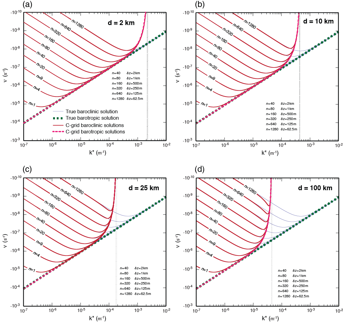
3.2 Solutions for the C grid

Baroclinic Rossby modes. We horizontally discretize Eqs. (1) and (2) on the C grid shown in Fig. 1b of Part 1 as

$$\begin{array}{ll}{\displaystyle }& {\displaystyle \frac{\partial {\left({\mathit{\omega }}_z\right)}_{i+\mathrm{1}/\mathrm{2},j+\mathrm{1}/\mathrm{2}}}{\partial t}}=\\ {\displaystyle }& {\displaystyle }-f_{\mathrm{0}}{\displaystyle \frac{\mathrm{1}}{\mathrm{4}}}\left(D_{i,j}+D_{i+\mathrm{1},j}+D_{i,j+\mathrm{1}}+D_{i+\mathrm{1},j+\mathrm{1}}\right)\\ \text{(16)}& {\displaystyle }& {\displaystyle }-{\displaystyle \frac{\mathit{\beta }}{f_{\mathrm{0}}}}\left({\displaystyle \frac{{\stackrel{\mathrm{‾}}{P}}_{i+\mathrm{3}/\mathrm{2},j+\mathrm{1}/\mathrm{2}}-{\stackrel{\mathrm{‾}}{P}}_{i-\mathrm{1}/\mathrm{2},j+\mathrm{1}/\mathrm{2}}}{\mathrm{2}d}}\right),\end{array}$$

where

$$\begin{array}{ll}\text{(17)}& {\displaystyle }& {\displaystyle }{\stackrel{\mathrm{‾}}{P}}_{i+\mathrm{1}/\mathrm{2},j+\mathrm{1}/\mathrm{2}}\equiv {\displaystyle }& {\displaystyle \frac{\mathrm{1}}{\mathrm{4}}}\left(P_{i,j}+P_{i+\mathrm{1},j}+P_{i,j+\mathrm{1}}+P_{i+\mathrm{1},j+\mathrm{1}}\right),\\ {\displaystyle }& {\displaystyle }\text{and}\\ {\displaystyle }& {\displaystyle }\mathrm{0}=\\ {\displaystyle }& {\displaystyle }{f}_{\mathrm{0}}{\displaystyle \frac{\mathrm{1}}{\mathrm{4}}}\left[{\left({\mathit{\omega }}_z\right)}_{i+\mathrm{1}/\mathrm{2},j+\mathrm{1}/\mathrm{2}}+{\left({\mathit{\omega }}_z\right)}_{i+\mathrm{1}/\mathrm{2},j-\mathrm{1}/\mathrm{2}}+{\left({\mathit{\omega }}_z\right)}_{i-\mathrm{1}/\mathrm{2},j+\mathrm{1}/\mathrm{2}}\right.\\ {\displaystyle }& {\displaystyle }\left.+{\left({\mathit{\omega }}_z\right)}_{i-\mathrm{1}/\mathrm{2},j-\mathrm{1}/\mathrm{2}}\right]-{\displaystyle \frac{\mathrm{1}}{d^{\mathrm{2}}}}\left(P_{i+\mathrm{1},j}+P_{i-\mathrm{1},j}+P_{i,j+\mathrm{1}}\right.\\ {\displaystyle }& {\displaystyle }\left.+P_{i,j-\mathrm{1}}-\mathrm{4}{P}_{i,j}\right).\end{array}$$

Equations (16), (17) and (10) complete the set of discrete equations for the C grid. By using Eqs. (16) and (22) of Part 1, we obtain the discrete dispersion relation as

$$\begin{array}{}\text{(18)}& \mathit{\nu }={\displaystyle \frac{-{\mathit{\mu }}^{\mathrm{2}}\stackrel{\mathrm{̃}}{\mathit{\xi }}\mathit{\beta }k}{{\mathit{\xi }}^{\mathrm{2}}{k}^{\mathrm{2}}+{\mathit{\eta }}^{\mathrm{2}}{\mathrm{\ell }}^{\mathrm{2}}+\frac{{\mathit{\mu }}^{\mathrm{2}}{f}_{\mathrm{0}}^{\mathrm{2}}}{N^{\mathrm{2}}}\left(m^{\mathrm{2}}+\frac{\mathrm{1}}{\mathrm{4}{H}^{\mathrm{2}}}\right)}},\end{array}$$

where $\stackrel{\mathrm{̃}}{\mathit{\xi }}$, ξ and η are given by Eq. (12), and

$$\begin{array}{}\text{(19)}& \mathit{\mu }\equiv \cos \left({\displaystyle \frac{\mathrm{1}}{\mathrm{2}}}kd\right)\cos \left({\displaystyle \frac{\mathrm{1}}{\mathrm{2}}}\mathrm{\ell }d\right).\end{array}$$

The definition of μ is identical to that used in Part 1.

Barotropic Rossby modes. By using D=0 in Eqs. (16) and (17) and then using Eqs. (16) and (22) of Part 1, we obtain the discrete dispersion relation for barotropic Rossby modes on the C grid as

$$\begin{array}{}\text{(20)}& \mathit{\nu }={\displaystyle \frac{-{\mathit{\mu }}^{\mathrm{2}}\stackrel{\mathrm{̃}}{\mathit{\xi }}\mathit{\beta }k}{{\mathit{\xi }}^{\mathrm{2}}{k}^{\mathrm{2}}+{\mathit{\eta }}^{\mathrm{2}}{\mathrm{\ell }}^{\mathrm{2}}}}.\end{array}$$

The discrete baroclinic and barotropic dispersion relations, Eqs. (18) and (20), for the C grid include an averaging factor μ². This is a difference from their Z-grid counterparts, Eqs. (11) and (15). Averaging of pressure term P from the cell centers to the corners in Eq. (17) leads to the factor of μ² in the numerators of Eqs. (18) and (20). A factor of μ² also appears in the inertia term at the denominator of Eq. (18), due to the averaging of divergence and vorticity to each other's grid points. Since μ and $\stackrel{\mathrm{̃}}{\mathit{\xi }}$ are both equal to zero at the SRZS, dynamically inert modes exist for both the baroclinic and barotropic Rossby modes on the C grid, similar to those that exist in the Z-grid solutions.

The C-grid solutions shown in Fig. 2 are qualitatively similar to the Z-grid solutions, but the C-grid solution deviates slightly because the dispersion relation for the C grid given by Eq. (18) contains an averaging factor μ² in the numerator. Since μ also approaches zero at the SRZS, and $\stackrel{\mathrm{̃}}{\mathit{\xi }}$ approaches zero, the small-scale modes on the C grid move or oscillate more slowly than on the Z grid. As mentioned above, at the SRZS, a dynamically inert mode is generated with the C grid.

3.3 Solutions for the D grid

Baroclinic Rossby modes. We horizontally discretize Eqs. (1) and (2) on the D grid shown in Fig. 1c of Part 1 as

$$\begin{array}{ll}\text{(21)}& {\displaystyle }& {\displaystyle \frac{\partial {\left({\mathit{\omega }}_z\right)}_{i,j}}{\partial t}}={\displaystyle }& {\displaystyle }-f_{\mathrm{0}}{\displaystyle \frac{\mathrm{1}}{\mathrm{4}}}\left(D_{i-\mathrm{1}/\mathrm{2},j-\mathrm{1}/\mathrm{2}}+D_{i+\mathrm{1}/\mathrm{2},j-\mathrm{1}/\mathrm{2}}+D_{i-\mathrm{1}/\mathrm{2},j+\mathrm{1}/\mathrm{2}}\right.\\ {\displaystyle }& {\displaystyle }\left.+D_{i+\mathrm{1}/\mathrm{2},j+\mathrm{1}/\mathrm{2}}\right)-{\displaystyle \frac{\mathit{\beta }}{f_{\mathrm{0}}}}{\displaystyle \frac{P_{i+\mathrm{1},j}-P_{i-\mathrm{1},j}}{\mathrm{2}d}},\end{array}$$

and

$$\begin{array}{ll}\text{(22)}& {\displaystyle }& {\displaystyle }\mathrm{0}={\displaystyle }& {\displaystyle }{f}_{\mathrm{0}}{\displaystyle \frac{\mathrm{1}}{\mathrm{4}}}\left[{\left({\mathit{\omega }}_z\right)}_{i+\mathrm{1},j+\mathrm{1}}+{\left({\mathit{\omega }}_z\right)}_{i,j+\mathrm{1}}+{\left({\mathit{\omega }}_z\right)}_{i+\mathrm{1},j}+{\left({\mathit{\omega }}_z\right)}_{i,j}\right]\\ {\displaystyle }& {\displaystyle }-{\displaystyle \frac{\mathrm{1}}{d^{\mathrm{2}}}}\left({\stackrel{\mathrm{‾}}{P}}_{i+\mathrm{3}/\mathrm{2},j+\mathrm{1}/\mathrm{2}}+{\stackrel{\mathrm{‾}}{P}}_{i+\mathrm{1}/\mathrm{2},j+\mathrm{3}/\mathrm{2}}+{\stackrel{\mathrm{‾}}{P}}_{i+\mathrm{1}/\mathrm{2},j-\mathrm{1}/\mathrm{2}}\right.\\ {\displaystyle }& {\displaystyle }\left.+{\stackrel{\mathrm{‾}}{P}}_{i-\mathrm{1}/\mathrm{2},j+\mathrm{1}/\mathrm{2}}-\mathrm{4}{\stackrel{\mathrm{‾}}{P}}_{i+\mathrm{1}/\mathrm{2},j+\mathrm{1}/\mathrm{2}}\right),\end{array}$$

respectively. In Eq. (22), ${\stackrel{\mathrm{‾}}{P}}_{i+\mathrm{1}/\mathrm{2},j+\mathrm{1}/\mathrm{2}}\equiv \frac{\mathrm{1}}{\mathrm{4}}\left(P_{i,j}+P_{i+\mathrm{1},j}+P_{i,j+\mathrm{1}}+P_{i+\mathrm{1},j+\mathrm{1}}\right)$. By adding the discrete version of Eq. (3) given by

$$\begin{array}{ll}\text{(23)}& {\displaystyle }& {\displaystyle }{N}^{\mathrm{2}}\left[{\displaystyle \frac{\mathrm{1}}{\mathrm{4}}}\left(D_{i-\mathrm{1}/\mathrm{2},j-\mathrm{1}/\mathrm{2}}+D_{i+\mathrm{1}/\mathrm{2},j-\mathrm{1}/\mathrm{2}}+D_{i-\mathrm{1}/\mathrm{2},j+\mathrm{1}/\mathrm{2}}\right.\right.{\displaystyle }& {\displaystyle }\left.\left.+D_{i+\mathrm{1}/\mathrm{2},j+\mathrm{1}/\mathrm{2}}\right)\right]-\left[{\displaystyle \frac{{\partial }^{\mathrm{2}}}{\partial z^{\mathrm{2}}}}-{\left({\displaystyle \frac{\mathrm{1}}{\mathrm{2}{\mathit{\rho }}_{\mathrm{0}}}}{\displaystyle \frac{\partial {\mathit{\rho }}_{\mathrm{0}}}{\partial z}}\right)}^{\mathrm{2}}\right]{\displaystyle \frac{\partial }{\partial t}}{P}_{i,j}=\mathrm{0}\end{array}$$

to Eqs. (21) and (22), we complete the discrete equations for the D grid. The resulting discrete dispersion relation is

$$\begin{array}{}\text{(24)}& \mathit{\nu }={\displaystyle \frac{-\stackrel{\mathrm{̃}}{\mathit{\xi }}\mathit{\beta }k}{{\mathit{\xi }}^{\mathrm{2}}{k}^{\mathrm{2}}+{\mathit{\eta }}^{\mathrm{2}}{\mathrm{\ell }}^{\mathrm{2}}+\frac{f_{\mathrm{0}}^{\mathrm{2}}}{N^{\mathrm{2}}}\left(m^{\mathrm{2}}+\frac{\mathrm{1}}{\mathrm{4}{H}^{\mathrm{2}}}\right)}}.\end{array}$$

Barotropic Rossby modes. By using D=0 in Eqs. (21) and (22), and using Eqs. (16) and (22) of Part 1, we obtain the discrete dispersion relation for the discrete barotropic modes as

$$\begin{array}{}\text{(25)}& \mathit{\nu }={\displaystyle \frac{-\stackrel{\mathrm{̃}}{\mathit{\xi }}\mathit{\beta }k}{{\mathit{\xi }}^{\mathrm{2}}{k}^{\mathrm{2}}+{\mathit{\eta }}^{\mathrm{2}}{\mathrm{\ell }}^{\mathrm{2}}}}.\end{array}$$

The dispersion equation for the discrete baroclinic and barotropic Rossby modes on the D grid is identical to that of the Z-grid solution. In the linear system, every averaging introduces a factor μ. For nontrivial solutions of Eqs. (21)–(23), the factors of μ cancel each other. As a result, the dispersion equation is identical to that of the Z grid.

Figure 1 is effectively a plot of the frequencies for the D grid because the dispersion equations for the Z grid given by Eqs. (11) and (15) are identical to those for the D grid, as given by Eqs. (24) and (25), respectively.

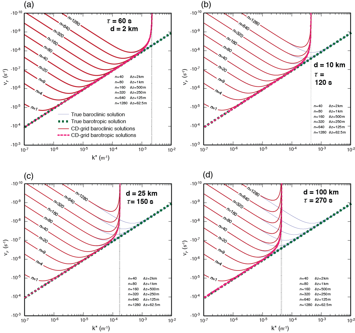
3.4 Solutions for the CD grid

Baroclinic Rossby modes. By dropping the finite-difference time derivatives of divergence and vertical velocity in Eqs. (32)–(42) of Part 1 and adding $-\underset{\sim }{i}\frac{\mathrm{1}}{\mathrm{2}}\mathit{\tau }\mathit{\mu }\left(\mathit{\beta }/f_{\mathrm{0}}\right)\stackrel{\mathrm{̃}}{\mathit{\xi }}k\widehat{P}$ and $-\underset{\sim }{i}\mathit{\tau }\left(\mathit{\beta }/f_{\mathrm{0}}\right)\stackrel{\mathrm{̃}}{\mathit{\xi }}k\widehat{P}$ to Eqs. (32) and (38) of Part 1, respectively, we write the CD-grid equations for a midlatitude β plane as

Predictor step on the C grid:

$$\begin{array}{}\text{(26)}& {\displaystyle }& {\displaystyle }{\widehat{\mathit{\omega }}}_z^{(*)}=\mathit{\mu }{\widehat{\mathit{\omega }}}_z^{\left(n\right)}-{\displaystyle \frac{\mathrm{1}}{\mathrm{2}}}\mathit{\tau }{f}_{\mathrm{0}}\widehat{D}-\underset{\sim }{i}{\displaystyle \frac{\mathrm{1}}{\mathrm{2}}}\mathit{\tau }\mathit{\mu }\left(\mathit{\beta }/f_{\mathrm{0}}\right)\stackrel{\mathrm{̃}}{\mathit{\xi }}k\widehat{P},\text{(27)}& {\displaystyle }& {\displaystyle }\mathrm{0}=f_{\mathrm{0}}{\widehat{w}}_z^{\left(n\right)}+L^{\mathrm{2}}\widehat{P},\text{(28)}& {\displaystyle }& {\displaystyle }\mathrm{0}=-\left(\underset{\sim }{i}m+{\displaystyle \frac{\mathrm{1}}{\mathrm{2}H}}\right)\widehat{P}+{\widehat{B}}^{\left(n\right)},\text{(29)}& {\displaystyle }& {\displaystyle }{\widehat{B}}^{(*)}={\widehat{B}}^{\left(n\right)}-{\displaystyle \frac{\mathrm{1}}{\mathrm{2}}}\mathit{\tau }{N}^{\mathrm{2}}\widehat{w},\text{(30)}& {\displaystyle }& {\displaystyle }\widehat{D}+\left(\underset{\sim }{i}m-{\displaystyle \frac{\mathrm{1}}{\mathrm{2}H}}\right)\widehat{w}=\mathrm{0}.\end{array}$$

Corrector step on the D grid:

$$\begin{array}{}\text{(31)}& {\displaystyle }& {\displaystyle }{\widehat{\mathit{\omega }}}_z^{\left(n+\mathrm{1}\right)}={\widehat{\mathit{\omega }}}_z^{\left(n\right)}-\mathit{\tau }{f}_{\mathrm{0}}\mathit{\mu }\widehat{D}-\underset{\sim }{i}\mathit{\tau }\left(\mathit{\beta }/f_{\mathrm{0}}\right)\stackrel{\mathrm{̃}}{\mathit{\xi }}k\widehat{P},\text{(32)}& {\displaystyle }& {\displaystyle }\mathrm{0}=f_{\mathrm{0}}{\widehat{w}}_z^{\left(n\right)}+\mathit{\mu }{L}^{\mathrm{2}}\widehat{P},\text{(33)}& {\displaystyle }& {\displaystyle }\mathrm{0}=-\left(\underset{\sim }{i}m+{\displaystyle \frac{\mathrm{1}}{\mathrm{2}H}}\right)\widehat{P}+{\widehat{B}}^{(*)},\text{(34)}& {\displaystyle }& {\displaystyle }{\widehat{B}}^{\left(n+\mathrm{1}\right)}={\widehat{B}}^{\left(n\right)}-\mathit{\tau }{N}^{\mathrm{2}}\widehat{w},\text{(35)}& {\displaystyle }& {\displaystyle }\mathit{\mu }\widehat{D}+\left(\underset{\sim }{i}m-{\displaystyle \frac{\mathrm{1}}{\mathrm{2}H}}\right)\widehat{w}=\mathrm{0}.\end{array}$$

In these equations, $\stackrel{\mathrm{̃}}{\mathit{\xi }}$ is given by Eq. (12), $L^{\mathrm{2}}\equiv {\mathit{\xi }}^{\mathrm{2}}{k}^{\mathrm{2}}+{\mathit{\eta }}^{\mathrm{2}}{\mathrm{\ell }}^{\mathrm{2}}$, ξ and η are given by Eq. (12) and μ is given by Eq. (15).

In this system, the divergence is a diagnostic variable, defined on the cell corners. This is why the divergence $\widehat{D}$ is multiplied by the averaging factor μ in Eq. (31) but not in Eq. (26). Using Scheme I, as discussed in Part 1, we eliminate ${\widehat{\mathit{\omega }}}_z^{(\ast )}$ by using Eq. (26) in Eq. (32) and eliminate ${\widehat{B}}^{(\ast )}$ by using Eq. (29) in Eq. (33). Then Eq. (43) of Part 1 is used to obtain the real frequency and amplification factor equations as follows:

$$\begin{array}{ll}\text{(36)}& {\displaystyle }& {\displaystyle }{e}^{\mathrm{2}{\mathit{\nu }}_i\mathit{\tau }}\left({\mathit{\mu }}^{\mathrm{2}}{N}^{\mathrm{2}}{L}^{\mathrm{2}}+f_{\mathrm{0}}^{\mathrm{2}}{\mathit{\sigma }}_m^{\mathrm{2}}\right)\sin \left(\mathrm{2}{\mathit{\nu }}_r\mathit{\tau }\right){\displaystyle }& {\displaystyle }+{\displaystyle \frac{\mathrm{1}}{\mathrm{2}}}\mathit{\tau }{e}^{\mathrm{2}{\mathit{\nu }}_i\mathit{\tau }}{\mathit{\mu }}^{\mathrm{2}}{N}^{\mathrm{2}}\mathit{\beta }\stackrel{\mathrm{̃}}{\mathit{\xi }}\cos \left(\mathrm{2}{\mathit{\nu }}_r\mathit{\tau }\right)+\mathit{\tau }{e}^{{\mathit{\nu }}_i\mathit{\tau }}{\mathit{\mu }}^{\mathrm{2}}{N}^{\mathrm{2}}\cos \left({\mathit{\nu }}_r\mathit{\tau }\right)\mathit{\beta }\stackrel{\mathrm{̃}}{\mathit{\xi }}k\\ {\displaystyle }& {\displaystyle }+\mathrm{2}{f}_{\mathrm{0}}^{\mathrm{2}}{e}^{{\mathit{\nu }}_i\mathit{\tau }}\left({\mathit{\mu }}^{\mathrm{2}}-\mathrm{1}\right){\mathit{\sigma }}_m^{\mathrm{2}}\sin \left({\mathit{\nu }}_r\mathit{\tau }\right)+{\displaystyle \frac{\mathrm{1}}{\mathrm{2}}}\mathit{\tau }{\mathit{\mu }}^{\mathrm{2}}{N}^{\mathrm{2}}\mathit{\beta }\stackrel{\mathrm{̃}}{\mathit{\xi }}k=\mathrm{0},\end{array}$$

and

$$\begin{array}{}\text{(37)}& e^{{\mathit{\nu }}_i\mathit{\tau }}={\displaystyle \frac{-b+\sqrt{b^{\mathrm{2}}-\mathrm{4}ac}}{\mathrm{2}a}},\end{array}$$

where

$$\begin{array}{ll}\text{(38a)}& {\displaystyle }a\equiv & {\displaystyle }{\mathit{\mu }}^{\mathrm{2}}{N}^{\mathrm{2}}{L}^{\mathrm{2}}\cos \left(\mathrm{2}{\mathit{\nu }}_r\mathit{\tau }\right)-{\displaystyle \frac{\mathrm{1}}{\mathrm{2}}}\mathit{\tau }{\mathit{\mu }}^{\mathrm{2}}{N}^{\mathrm{2}}\mathit{\beta }\stackrel{\mathrm{̃}}{\mathit{\xi }}k\sin \left(\mathrm{2}{\mathit{\nu }}_r\mathit{\tau }\right){\displaystyle }& {\displaystyle }+f_{\mathrm{0}}^{\mathrm{2}}{\mathit{\sigma }}_m^{\mathrm{2}}\cos \left(\mathrm{2}{\mathit{\nu }}_r\mathit{\tau }\right),\\ \text{(38b)}& {\displaystyle }b\equiv & {\displaystyle }\mathrm{2}{f}_{\mathrm{0}}^{\mathrm{2}}\left({\mathit{\mu }}^{\mathrm{2}}-\mathrm{1}\right){\mathit{\sigma }}_m^{\mathrm{2}}\cos \left({\mathit{\nu }}_r\mathit{\tau }\right){\displaystyle }& {\displaystyle }-\mathit{\tau }{\mathit{\mu }}^{\mathrm{2}}{N}^{\mathrm{2}}\mathit{\beta }\stackrel{\mathrm{̃}}{\mathit{\xi }}k\sin \left({\mathit{\nu }}_r\mathit{\tau }\right),\end{array}$$

and

$$\begin{array}{}\text{(38c)}& c\equiv f_{\mathrm{0}}^{\mathrm{2}}\left(\mathrm{1}-\mathrm{2}{\mathit{\mu }}^{\mathrm{2}}\right){\mathit{\sigma }}_m^{\mathrm{2}}-{\mathit{\mu }}^{\mathrm{2}}{N}^{\mathrm{2}}{L}^{\mathrm{2}}.\end{array}$$

Barotropic Rossby modes. By eliminating the divergence, vertical velocity and buoyancy in Eqs. (26)–(35), we obtain the two-part dispersion equation for the barotropic modes as

$$\begin{array}{ll}\text{(39)}& {\displaystyle }\mathrm{0}=& {\displaystyle }\left[{\left(L^{\mathrm{2}}\right)}^{\mathrm{2}}-{\left({\displaystyle \frac{\mathrm{1}}{\mathrm{2}}}\mathit{\tau }\mathit{\beta }\stackrel{\mathrm{̃}}{\mathit{\xi }}k\right)}^{\mathrm{2}}\right]\sin \left({\mathit{\nu }}_r\mathit{\tau }\right){\displaystyle }& {\displaystyle }+\mathit{\tau }\mathit{\beta }\stackrel{\mathrm{̃}}{\mathit{\xi }}k{L}^{\mathrm{2}}\cos \left({\mathit{\nu }}_r\mathit{\tau }\right),\end{array}$$

and

$$\begin{array}{}\text{(40)}& e^{{\mathit{\nu }}_i\mathit{\tau }}={\displaystyle \frac{L^{\mathrm{2}}}{L^{\mathrm{2}}\cos \left({\mathit{\nu }}_r\mathit{\tau }\right)-\frac{\mathrm{1}}{\mathrm{2}}\mathit{\tau }\mathit{\beta }\stackrel{\mathrm{̃}}{\mathit{\xi }}k\sin \left({\mathit{\nu }}_r\mathit{\tau }\right)}}.\end{array}$$

At the SRZS, for which $\stackrel{\mathrm{̃}}{\mathit{\xi }}=\mathrm{0}$ and μ=0, the real frequency ν_r becomes 0 in Eqs. (36) and (39), and the amplification factor $e^{{\mathit{\nu }}_i\mathit{\tau }}$ becomes 1 in Eqs. (37) and (40). The Supplement gives a more detailed derivation of the discrete equations.

The CD-grid solution shown by Fig. 3 is virtually identical to that for the Z-grid solutions (and D-grid solutions) shown in Figs. 1 and 2, respectively.

Figure 3 Same as Fig. 1 but on the CD grid.

DC grid

As stated above, the CD grid behaves similarly to the D grid rather than the C grid in the numerical solution of the Rossby waves on a midlatitude β plane. The normal-mode analysis of the Rossby waves with the DC grid produce a solution that is very close to the C-grid solution. A detailed discussion and frequency plots are presented in the Supplement. This is consistent with the findings of Part 1 that the correction step dominates the solutions with the CD and DC grids.

3.5 Solutions for the A grid

Baroclinic Rossby modes. We horizontally discretize Eqs. (1)–(3) on the A grid shown in Fig. 1e of Part 1 as

$$\begin{array}{}\text{(41)}& {\displaystyle \frac{\partial }{\partial t}}{\left({\mathit{\omega }}_z\right)}_{i,j}=-f_{\mathrm{0}}{D}_{i,j}-{\displaystyle \frac{\mathit{\beta }}{f_{\mathrm{0}}}}{\displaystyle \frac{P_{i+\mathrm{1},j}-P_{i-\mathrm{1},j}}{\mathrm{2}d}},\end{array}$$

and

$$\begin{array}{ll}\text{(42)}& {\displaystyle }& {\displaystyle }\mathrm{0}={\displaystyle }& {\displaystyle }f{\left({\mathit{\omega }}_z\right)}_{i,j}-{\displaystyle \frac{\mathrm{1}}{\mathrm{4}{d}^{\mathrm{2}}}}\left(P_{i+\mathrm{2},j}+P_{i,j+\mathrm{2}}+P_{i,j-\mathrm{2}}+P_{i-\mathrm{2},j}-\mathrm{4}{P}_{i,j}\right),\end{array}$$

respectively. Similarly, we obtain the discrete dispersion relation for the baroclinic Rossby modes as

$$\begin{array}{}\text{(43)}& {\displaystyle }\mathit{\nu }={\displaystyle \frac{-\mathit{\beta }\stackrel{\mathrm{̃}}{\mathit{\xi }}k}{{\stackrel{\mathrm{̃}}{\mathit{\xi }}}^{\mathrm{2}}{k}^{\mathrm{2}}+{\stackrel{\mathrm{̃}}{\mathit{\eta }}}^{\mathrm{2}}{\mathrm{\ell }}^{\mathrm{2}}+\frac{f_{\mathrm{0}}^{\mathrm{2}}}{N^{\mathrm{2}}}\left(m^{\mathrm{2}}+\frac{\mathrm{1}}{\mathrm{4}{H}^{\mathrm{2}}}\right)}},\end{array}$$

where the definition of $\stackrel{\mathrm{̃}}{\mathit{\xi }}$ is given by Eq. (12) and

$$\begin{array}{}\text{(44)}& \stackrel{\mathrm{̃}}{\mathit{\eta }}\equiv {\displaystyle \frac{\sin \left(\mathrm{\ell }d\right)}{\mathrm{\ell }d}}.\end{array}$$

The frequency becomes zero at the SRZS because $\stackrel{\mathrm{̃}}{\mathit{\xi }}$ is zero in the nominator of Eq. (43). This indicates the existence of a non-moving and non-oscillating computational mode. Moreover, the factor of ${\stackrel{\mathrm{̃}}{\mathit{\xi }}}^{\mathrm{2}}$ in the denominator causes the frequency to behave badly near the smallest resolvable horizontal scale.

Barotropic Rossby modes. By dropping $\left(f_{\mathrm{0}}^{\mathrm{2}}/N^{\mathrm{2}}\right)\left(m^{\mathrm{2}}+\mathrm{1}/\mathrm{4}{H}^{\mathrm{2}}\right)$ in Eq. (43), the discrete dispersion relation for the barotropic Rossby modes can be obtained as

$$\begin{array}{}\text{(45)}& \mathit{\nu }={\displaystyle \frac{-\mathit{\beta }\stackrel{\mathrm{̃}}{\mathit{\xi }}k}{{\stackrel{\mathrm{̃}}{\mathit{\xi }}}^{\mathrm{2}}{k}^{\mathrm{2}}+{\stackrel{\mathrm{̃}}{\mathit{\eta }}}^{\mathrm{2}}{\mathrm{\ell }}^{\mathrm{2}}}}.\end{array}$$

The frequency of the barotropic modes becomes strongly negative (retrogressing) at the SRZS. This means that small-scale barotropic Rossby modes can behave very badly. We discuss the behavior of these modes in connection with the plots below.

Figure 4 Same as Fig. 1 but on the A grid.

Figure 5 Same as Fig. 1 but on the E grid.

Figure 6 Same as Fig. 1 but on the B grid.

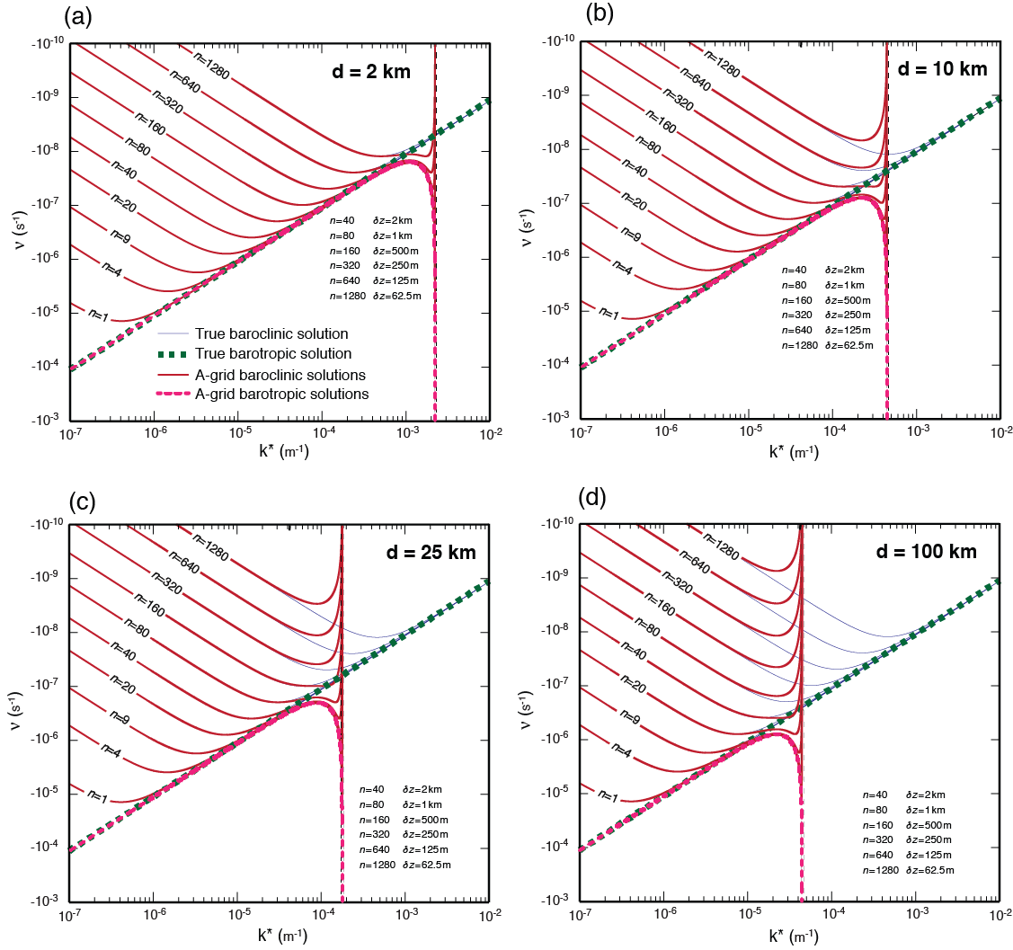
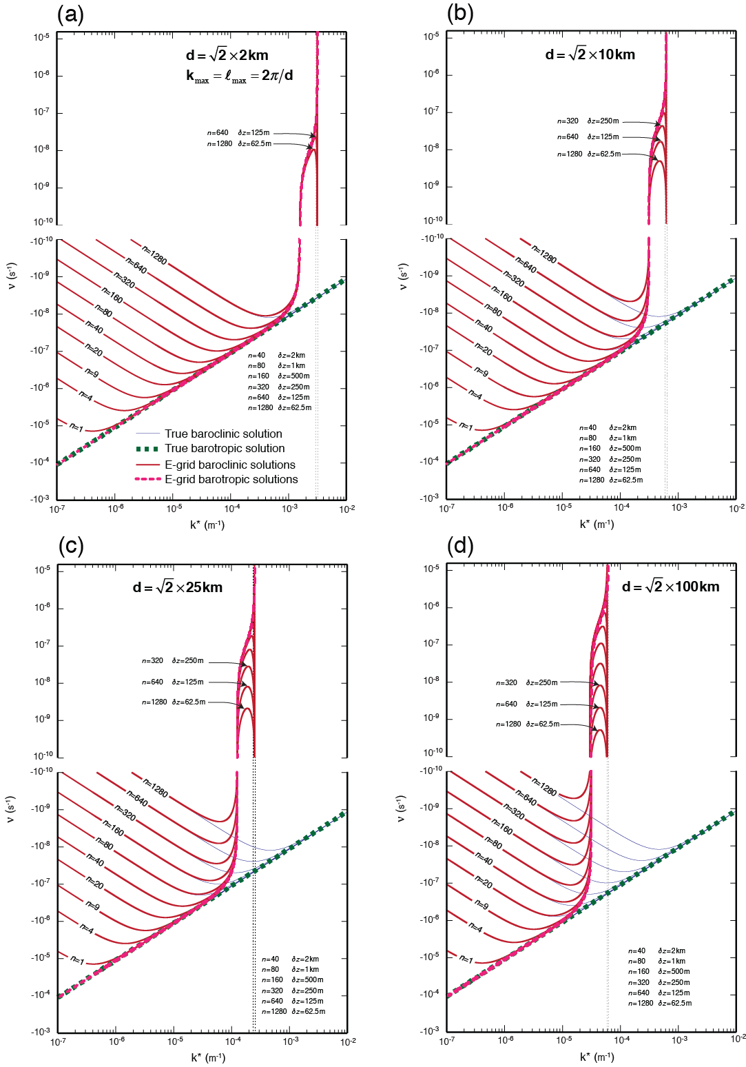
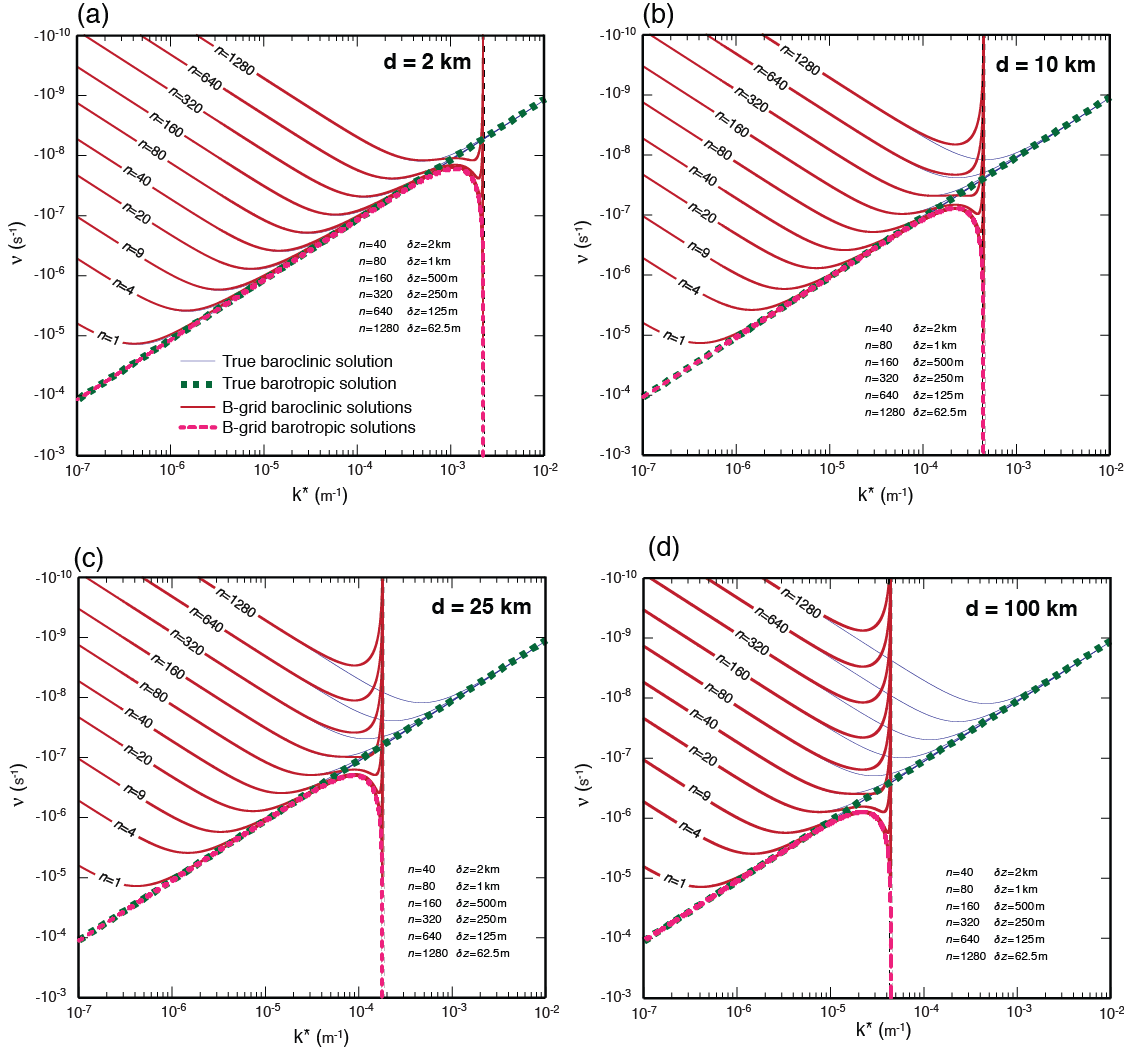
Figure 4 shows the frequency of the Rossby modes obtained on the A grid. The A grid produces very fast retrogression speeds of the barotropic mode at the SRZS. The baroclinic modes with short vertical scales retrograde faster than the true solution near the SRZS, but right at the SRZS, they do not move at all.

3.6 Baroclinic and barotropic Rossby modes with the E grid

Part 1 discusses in detail the horizontal discretization on the E grid. There it is pointed out that the E grid can be viewed as the superposition of the two C grids, in which the cell centers of one C grid are placed at the corners of a second C grid. It is also shown that, from the vorticity and divergence point of view, the E grid can be viewed as a superposition of two independent and non-interacting Z grids, as shown in Fig. 1f of Part 1. The dispersion relation for the E grid is identical to that for the Z grid, but the smallest resolvable zonal scale extends to $k_{max}=\mathrm{2}\mathit{\pi }/d$ (and ${\mathrm{\ell }}_{max}=\mathrm{2}\mathit{\pi }/d)$ for the E grid. Therefore, the dispersions of baroclinic and barotropic modes on the E grid are governed by Eqs. (11) and (15) with k_max and ℓ_max as described above. Recall that we use a grid spacing of $\sqrt{\mathrm{2}}d$ with the E grid to maintain the same cell density as with the other grids.

The E grid produces the wildest solutions, as shown in Fig. 5. It is the only grid that generates prograding Rossby modes. The modes with all vertical scales and horizontal grid spacings used in the models generate prograding solutions near the SRZS. The deeper the mode is, the faster the progradation speed is. The prograding modes are generated near the SRZS because the factor $\stackrel{\mathrm{̃}}{\mathit{\xi }}$ yields negative values for $k>\mathit{\pi }/d$. A interpretation is that the finite-difference pressure gradient determined over the two-grid distance is subject to aliasing errors for zonal waves with $k>\mathit{\pi }/d$, which causes the system to recognize the pressure gradient with the wrong sign.

3.7 Solutions for the B grid

Baroclinic Rossby modes. We can obtain the equations for the B grid by ignoring $\partial D/\partial t$ in Eq. (63) of Part 1, replacing f with f₀ and using Eqs. (8) and (9). Similarly, we obtain the discrete dispersion relation for the baroclinic Rossby modes on the B grid as

$$\begin{array}{}\text{(46)}& \mathit{\nu }={\displaystyle \frac{-\stackrel{\mathrm{̃}}{\mathit{\xi }}\mathit{\beta }k}{{\mathit{\xi }}^{\mathrm{2}}{k}^{\mathrm{2}}+{\mathit{\eta }}^{\mathrm{2}}{\mathrm{\ell }}^{\mathrm{2}}-\frac{\mathrm{1}}{\mathrm{2}}{d}^{\mathrm{2}}{\mathit{\xi }}^{\mathrm{2}}{k}^{\mathrm{2}}{\mathit{\eta }}^{\mathrm{2}}{\mathrm{\ell }}^{\mathrm{2}}+\frac{f_{\mathrm{0}}}{N^{\mathrm{2}}}\left(m^{\mathrm{2}}+\frac{\mathrm{1}}{\mathrm{4}{H}^{\mathrm{2}}}\right)}},\end{array}$$

where the factors ξ, η and $\stackrel{\mathrm{̃}}{\mathit{\xi }}$ are defined by Eq. (12). The frequency becomes zero for the SRZS because $\stackrel{\mathrm{̃}}{\mathit{\xi }}$ is zero. The Laplacian term ${\mathit{\xi }}^{\mathrm{2}}{k}^{\mathrm{2}}+{\mathit{\eta }}^{\mathrm{2}}{\mathrm{\ell }}^{\mathrm{2}}-\frac{\mathrm{1}}{\mathrm{2}}{d}^{\mathrm{2}}{\mathit{\xi }}^{\mathrm{2}}{k}^{\mathrm{2}}{\mathit{\eta }}^{\mathrm{2}}{\mathrm{\ell }}^{\mathrm{2}}$ also approaches zero in the numerator of Eq. (46) as the zonal wavenumber approaches the SRZS. This makes the frequency behave similarly to that of the A grid.

Barotropic Rossby modes. By dropping $\left(f_{\mathrm{0}}^{\mathrm{2}}/N^{\mathrm{2}}\right)\left(m^{\mathrm{2}}+\mathrm{1}/\mathrm{4}{H}^{\mathrm{2}}\right)$ in Eq. (46), we obtain the discrete dispersion relation of the barotropic Rossby modes as

$$\begin{array}{}\text{(47)}& \mathit{\nu }={\displaystyle \frac{-\stackrel{\mathrm{̃}}{\mathit{\xi }}\mathit{\beta }k}{{\mathit{\xi }}^{\mathrm{2}}{k}^{\mathrm{2}}+{\mathit{\eta }}^{\mathrm{2}}{\mathrm{\ell }}^{\mathrm{2}}-\frac{\mathrm{1}}{\mathrm{2}}{d}^{\mathrm{2}}{\mathit{\xi }}^{\mathrm{2}}{k}^{\mathrm{2}}{\mathit{\eta }}^{\mathrm{2}}{\mathrm{\ell }}^{\mathrm{2}}}}.\end{array}$$

The denominator approaches zero at the SRZS, which yields an infinite retrogression speed for these modes.

Figure 6 shows the frequency of the Rossby modes on the B grid. As with the A-grid solutions, the B grid produces infinitely fast retrogression speeds for the barotropic mode at the SRZS, and the shallow baroclinic modes retrograde faster than the true solution near the SRZS and do not move at all at the SRZS.

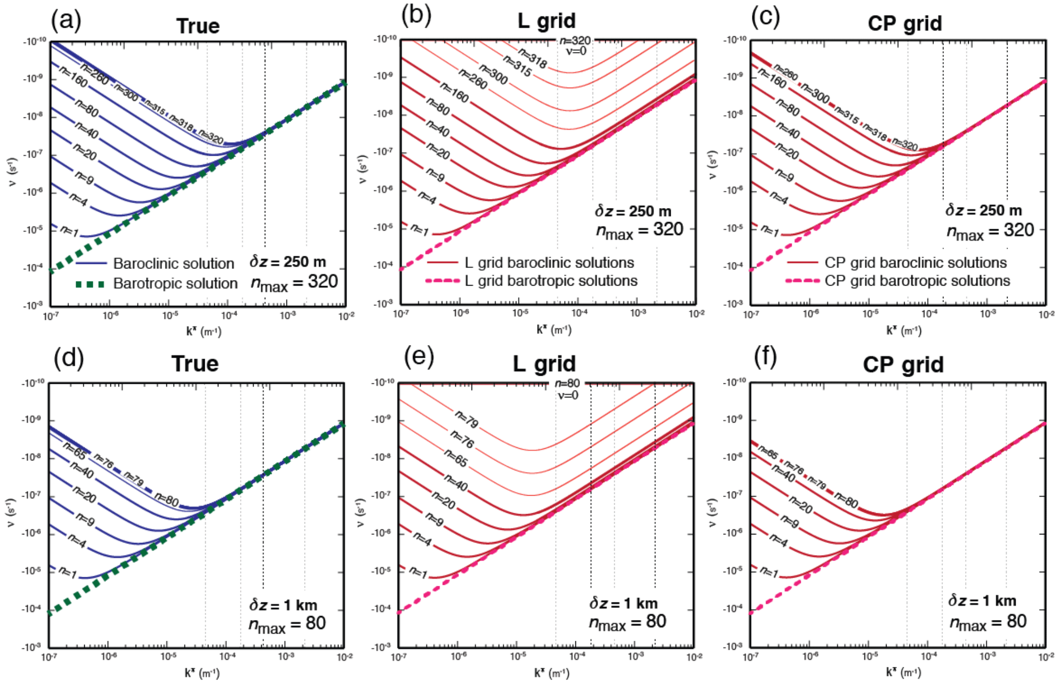
Figure 7 Plots of (a, d) true and discrete frequencies for the baroclinic and barotropic Rossby modes obtained on the (b, e) L and (c, f) CP grids. The thick blue and green dashed lines on the left panels indicate the true baroclinic and barotropic frequencies, respectively. The thick red and red dashed lines on the center and right panels indicate the discrete baroclinic and barotropic frequencies, respectively. The upper and lower panels show the plots for the maximum vertical integer wavenumbers of $n_{max}=\mathrm{320}$ (δz=250 m) and $n_{max}=\mathrm{80}$ (δz=1 km), respectively.

As discussed in Sect. 3.8 of Part 1, the A, E and B grids generate multiple (or non-unique) solutions and dynamically inert modes. Here, we see that the impact of the dynamically inert modes on the short Rossby waves is very severe.

The results of our normal-mode analysis of the nonhydrostatic anelastic barotropic and baroclinic Rossby waves on a midlatitude β plane the C, D, A, E and B grids overall agree with the results of Dukowicz's (1995) normal-mode analysis with the shallow-water equations. An exception is that we include the prograding modes with the E-grid solutions, whereas Dukowicz (1995) excludes them as “inadmissible”.

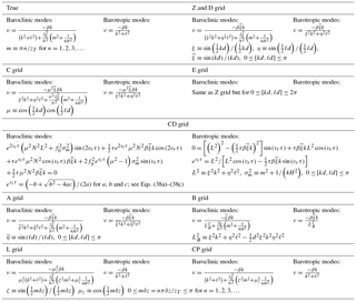
Table 1 A summary of the continuous and discrete dispersion relations with various horizontal and vertical grids.

3.8 Vertical discretization of the linear anelastic equations on the L and CP grids and discrete dispersion equation

Part 1 presents a discussion on the vertical grids, including a historical perspective, used in atmospheric models. Our purpose in this section is to assess and compare the performance of the L and CP grids in simulating Rossby modes on a midlatitude β plane through a normal-mode analysis.

3.9 The L grid

By replacing f with f₀ in Eqs. (65) and (66) of Part 1, adding the β term $-\left(\mathit{\beta }/f_{\mathrm{0}}\right)\left(\partial P_k/\partial x\right)$ to the right-hand side of Eq. (65) of Part 1 and dropping $\partial D_k/\partial t$ and $\partial w_{k+\mathrm{1}/\mathrm{2}}/\partial t$ in Eqs. (66) and (67) of Part 1, respectively, and using Eq. (70) of Part 1, we obtain (after some manipulations) the discrete dispersion relation for the baroclinic Rossby modes as

$$\begin{array}{}\text{(48)}& \mathit{\nu }={\displaystyle \frac{-{\mathit{\mu }}_z^{\mathrm{2}}\mathit{\beta }k}{{\mathit{\mu }}_z^{\mathrm{2}}\left(k^{\mathrm{2}}+{\mathrm{\ell }}^{\mathrm{2}}\right)+\frac{f_{\mathrm{0}}^{\mathrm{2}}}{N^{\mathrm{2}}}\left({\mathit{\zeta }}^{\mathrm{2}}{m}^{\mathrm{2}}+{\mathit{\mu }}_z^{\mathrm{2}}\frac{\mathrm{1}}{\mathrm{4}{H}^{\mathrm{2}}}\right)}},\end{array}$$

where

$$\begin{array}{}\text{(49)}& \mathit{\zeta }\equiv {\displaystyle \frac{\mathrm{1}}{\frac{\mathrm{1}}{\mathrm{2}}m\mathit{\delta }z}}\sin \left({\displaystyle \frac{\mathrm{1}}{\mathrm{2}}}m\mathit{\delta }z\right)\text{and}{\mathit{\mu }}_z\equiv \cos \left({\displaystyle \frac{\mathrm{1}}{\mathrm{2}}}m\mathit{\delta }z\right).\end{array}$$

By dropping $\left(f_{\mathrm{0}}^{\mathrm{2}}/N^{\mathrm{2}}\right)\left({\mathit{\zeta }}^{\mathrm{2}}{m}^{\mathrm{2}}+{\mathit{\mu }}_z^{\mathrm{2}}/\mathrm{4}{H}^{\mathrm{2}}\right)$ in Eq. (48), we obtain the discrete dispersion relation for the barotropic Rossby mode as

$$\begin{array}{}\text{(50)}& \mathit{\nu }={\displaystyle \frac{-\mathit{\beta }k}{k^{\mathrm{2}}+{\mathrm{\ell }}^{\mathrm{2}}}}.\end{array}$$

In Eq. (48), the numerator is proportional to ${\mathit{\mu }}_z^{\mathrm{2}}$, which is zero for the smallest resolvable vertical scale (SRVS), for which mδz=π. This means that, for all horizontal scales, the modes with the SRVS cannot propagate. They are dynamically inert (computational) modes. The pressure in the β term cannot recognize the SRVS buoyancy perturbation in the vertical velocity equation Eq. (67) of Part 1 with the quasi-static assumption ($\partial w_{k+\mathrm{1}/\mathrm{2}}/\partial t\approx \mathrm{0})$. The frequency of the discrete barotropic mode given by Eq. (50) is identical to the true frequency in Eq. (7), which is expected because the barotropic mode has no vertical structure and therefore is not affected by the vertical discretization.

3.10 The CP grid

We now derive the discrete dispersion relation for the baroclinic and barotropic Rossby modes on the CP grid, following the same strategy used with the L grid. The results are

$$\begin{array}{}\text{(51)}& \mathit{\nu }={\displaystyle \frac{-\mathit{\beta }k}{\left(k^{\mathrm{2}}+{\mathrm{\ell }}^{\mathrm{2}}\right)+\frac{f_{\mathrm{0}}^{\mathrm{2}}}{N^{\mathrm{2}}}\left({\mathit{\zeta }}^{\mathrm{2}}{m}^{\mathrm{2}}+{\mathit{\mu }}_z^{\mathrm{2}}\frac{\mathrm{1}}{\mathrm{4}{H}^{\mathrm{2}}}\right)}},\end{array}$$

and

$$\begin{array}{}\text{(52)}& \mathit{\nu }={\displaystyle \frac{-\mathit{\beta }k}{k^{\mathrm{2}}+{\mathrm{\ell }}^{\mathrm{2}}}},\end{array}$$

respectively. The dispersion equation for the baroclinic Rossby modes on the CP grid given by Eq. (51) does not have an averaging factor in the numerator, and therefore it does not allow a dynamically inert mode with zero frequency at the SRZS.

Figure 7 shows the frequencies as functions of composite horizontal wavenumber of barotropic and baroclinic Rossby modes obtained with the L and CP grids. The true frequencies are also shown in separate panels of the figure. The figure shows the results for two vertical wavenumbers (or number of layers), namely $n_{max}=\mathrm{320}$ and 80. We included additional frequency lines corresponding to more vertical wavenumbers than were used in the plots of Sect. 3 (indicated by thinner solid lines in the plots). In the L-grid solutions shown in Fig. 7b and e, the frequency of the smallest vertical resolvable mode, identified by n_max , deviates greatly from the true frequency, which yields zero values. Similar to the case of the inertia–gravity modes, as the vertical scale approaches the smallest resolvable scale, the modes gradually lose their ability to recognize the effects of buoyancy and therefore baroclinicity. For the mode with the smallest scale, the buoyancy and baroclinicity are completely decoupled from the wind field; for that mode, the buoyancy is dynamically inert. In contrast, the frequency of the CP-grid solutions shown in Fig. 7c and f is generally close to the true frequency but slightly higher.

4 Summary and conclusions

We have discussed the effects on the dispersion of middle-latitude Rossby waves of the horizontal and vertical discretizations of the quasi-geostrophic (quasi-static) linearized equations on the A, B, C, CD, (DC), D, E and Z horizontal grids and the L and CP vertical grids. We present a summary of the discrete dispersions of Rossby modes for the horizontal and vertical grids in Table 1 for an easy comparison.

The Z, C, D and CD (DC) grids generate similar dispersion of the baroclinic and barotropic Rossby modes. All have a dynamically inert mode at the SRZS because these scales cannot recognize the β effect. The dispersion equations for the A and B grids give infinite frequencies at the SHZS. Among all horizontal grids, the E grid produces the wildest solutions. The Rossby modes of all vertical scales near the SHZS prograde, while the true modes retrograde. The A, E and B grids generate multiple (non-unique) solutions, including dynamically inert (computational) modes. The impact of the computational modes on the short Rossby modes appears very severe on these grids.

The results of our normal-mode analysis of the Rossby waves for the C, D, A, E and B grids overall agree with the results of Dukowicz's (1995) normal-mode analysis with the shallow-water equations. Dukowicz (1995) considers the prograding modes with the E-grid solutions “inadmissible”, however, while we include them.

The selection of the vertical grid impacts the dispersion of the Rossby modes as much as the horizontal grid selection. The modes with the smallest resolvable vertical scale on the L grid do not retrograde. The CP-grid solutions are much more accurate than the L-grid solutions.