A Lagrangian particle tracking framework for the super-droplet method in SCALE-SDM 5.2.6-2.3.1: implementation and computational evaluation

Lagrangian particle histories provide a useful way to diagnose cloud-microphysical pathways in particle-based models, but their practical use in massively parallel super-droplet simulations depends on how particle identifiers, event records, output files, and post-processing workflows are implemented. This paper documents and evaluates a Lagrangian particle-tracking framework in SCALE-SDM 5.2.6-2.3.1. The framework includes forward tracking, backward tracking, and Two-Pass Hybrid Tracking (TPHT). Forward tracking saves the later states of super-droplets selected before or during a simulation. Backward tracking saves the rank and record location of each selected super-droplet's predecessor at the previous output time, so that post-processing can retrieve that record with an 𝒪(1) lookup instead of searching all super-droplets. Both methods use a common procedure to select all valid super-droplets, a random or height–radius-stratified sample, or an externally supplied target list. TPHT uses two integrations over the same physical time interval. The first records super-droplet identifiers when a chosen radius or coalescence condition is met. After duplicate identifiers are removed, the second starts from the same physical and random-number state and writes backward links only for this reduced set. Controlled computational tests are used to characterise runtime, peak random-access memory (RAM), storage (disk-output volume), the effect of output interval on file volume and mean write time, and sampling error and seed-to-seed variability. A three-dimensional DYCOMS-II RF02 stratocumulus case demonstrates TPHT. In this demonstration, the target criteria selected 19.3 % of the estimated valid super-droplet identities, corresponding to an estimated 5.2-fold reduction in retained backward output after temporary identifier files were removed. This factor is specific to the broad criteria used in this test; much larger reductions are possible for problems with sparser target populations. Agreement of the recorded coalescence events between the two integrations provided evidence of reproducibility under the tested configuration. The case study shows that TPHT can identify particles of interest and reconstruct their saved histories while reducing retained output. In future, the same approach could be applied to other history- or event-based questions, including entrainment and mixing, sedimentation, and ice-particle growth.

1 Introduction

Tracking the evolutionary history of moving objects is a common diagnostic approach in atmospheric science. Lagrangian particle dispersion models, such as HYSPLIT (Draxler and Hess, 1998; Stein et al., 2015) and FLEXPART (Pisso et al., 2019; Stohl et al., 2005), are widely used to examine the origins and destinations of air parcels and atmospheric constituents. These models illustrate the value of forward and backward trajectory analysis at macroscopic atmospheric scales.

A related concept in computer science is data provenance or lineage tracking, which records the transformations that lead from input data to a given output (Simmhan et al., 2005; Freire et al., 2008). In numerical simulations, such provenance information can support reproducibility, debugging, and interpretation by preserving the link between a diagnostic result and the intermediate states that produced it.

Applying these ideas to cloud microphysics requires additional model-specific choices. The Super-Droplet Method (SDM), a particle-based Lagrangian microphysics approach, has emerged as a state-of-the-art technique for simulating clouds with detailed microphysics, where each super-droplet represents a multitude of real particles (Shima et al., 2009, 2020). Although recent studies using SDM have presented the trajectories of cloud droplets and ice crystals as outcomes (Chandrakar et al., 2022, 2024), using such histories in a massively parallel SDM requires explicit choices for identifier definitions, MPI transfer, event logging, distributed output, post-processing reconstruction, and computational cost.

Other modelling approaches can also provide information on cloud-particle evolution, but with different compromises. Parcel models, for instance, track the motion and thermodynamic properties of a bulk air parcel and often rely on simplified assumptions such as adiabatic expansion and internal homogeneity (Krueger et al., 1997; Squires, 1958), thereby neglecting the individual histories and turbulent interactions of the droplets within. In contrast, the SDM framework allows for a more detailed examination of processes like condensation and collision-coalescence for individual super-droplets under realistic, turbulent conditions. Bin microphysics schemes track the evolution of the droplet size distribution by discretizing it into size bins (Khain et al., 2000, 2015). However, this approach is limited by the resolution of the bins, where important microphysical details may be averaged out, and numerical diffusion can artificially broaden the spectrum. SDM avoids these limitations by continuously following individual super-droplets, allowing for a more precise representation of their microphysical interactions without relying on binning. At the highest fidelity, Direct Numerical Simulation (DNS) is capable of tracking individual particles with exceptional resolution (Wang and Maxey, 1993; Ayala et al., 2008a, b), but its immense computational cost restricts its application to small domain sizes and low Reynolds numbers. This makes DNS impractical for studying cloud-scale structures where large eddies are crucial. SDM coupled with Large-Eddy Simulation (LES) provides an intermediate framework in which computational particles can be followed in cloud-scale turbulent simulations. For such simulations, the practical value of particle tracking depends not only on the tracking logic itself, but also on its output structure, memory footprint, I/O cost, and scalability. Therefore, a formally documented tracking algorithm capable of handling complex microphysical processes within a massively parallel SDM framework is still lacking in the literature.

Recent high-resolution SDM simulations have already used particle identifiers for diagnostic purposes. Matsushima et al. (2023) demonstrated the feasibility of metre- to submetre-scale simulations through high-performance computing optimisations. To validate their improved velocity interpolation scheme, they assigned a unique identifier to each super-droplet at the initial time and visualised particles according to their initial positions to analyse entrainment and mixing (e.g., their Fig. 6). This application demonstrates the value of persistent forward identifiers, but predecessor links through coalescence, event-level logging, distributed output, and the computational and storage implications of a broader tracking workflow were not central to that study. The present study documents and evaluates these elements in SCALE-SDM.

Particle-tracking diagnostics are particularly useful for questions in which particles are selected according to their histories, event participation, or later microphysical states. Examples include stochastic growth toward drizzle-size droplets, collision–coalescence participation, and entrainment or mixing histories, all of which have been studied previously (Telford, 1955; Dziekan and Pawlowska, 2017; Hoffmann et al., 2017; Li et al., 2022; Lim and Hoffmann, 2023, 2024). In the present paper, these studies motivate the use of event- and threshold-based target definitions, rather than serving as topics for a new process-level cloud-physics interpretation.

This paper presents a documented Lagrangian particle-tracking implementation in SCALE-SDM. The implementation provides three related workflows. Forward tracking assigns persistent identifiers to a chosen set of super-droplets and saves their later states. Backward tracking saves, for each selected record, where the corresponding predecessor can be found at the previous output time. The Two-Pass Hybrid Tracking (TPHT) combines two model integrations: the first identifies particles that meet prescribed radius or coalescence conditions, and the second starts from the same initial state and writes backward-linked histories only for those particles. The model also records event-level information for collision–coalescence. Separate post-processing tools use the saved identifiers to reconstruct selected histories from output files divided by MPI rank and model time. In addition to documenting these workflows, the paper evaluates wall-clock time, peak random-access memory (RAM), and output volume relative to simulations without tracking.

Full-population backward output preserves links for a broad set of super-droplets, allowing the final targets to be chosen after the simulation. This flexibility can require substantial disk output in large three-dimensional simulations. TPHT instead requires the selection conditions to be defined in advance and reconstructs histories only for particles that meet those conditions.

The remainder of this paper is organised as follows. Section 2 describes the SCALE-SDM implementation, including backward and forward tracking, the common procedure used to select tracked particles, and the TPHT workflow. Section 3 demonstrates the framework in a marine stratocumulus case based on DYCOMS-II RF02. The case study focuses on TPHT setup, computational cost, storage (disk-output volume) requirements, selected-particle statistics, recorded coalescence events, and example reconstructed histories. Section 4 discusses practical implications, limitations, and future extensions. Section 5 summarises the study. The appendices provide the controlled computational benchmark, the sampling-procedure verification, and the SDNC-scaling and output-interval sensitivity tests.

2 The Tracking Algorithms: Methodology and Implementation

2.1 General Framework: Numerical Model

The forward and backward tracking algorithms presented in this study were developed and implemented within the framework of the Scalable Computing for Advanced Library and Environment (SCALE) model, version 5.2.6 (Sato et al., 2015; Nishizawa et al., 2015). SCALE is an open-source software library jointly developed by institutions including the RIKEN (Institute of Physical and Chemical Research) Center for Computational Science and the Japan Meteorological Agency. It is designed to provide a flexible, efficient, and scalable numerical simulation platform for weather and climate research. Key features of the SCALE framework include a modular design, allowing users to combine various physical schemes to suit different research needs, and robust support for parallel computing (including MPI, OpenMP and OpenACC) to ensure high performance on diverse computational architectures.

For this work, we utilise SCALE-RM, the regional model component of the framework, whose dynamical core is based on the non-hydrostatic, compressible fluid equations. The model is configured as an LES, which explicitly resolves large-scale turbulent motions while parameterising unresolved small-scale turbulence using a sub-grid scale (SGS) model. This dynamical core is coupled with SDM, forming SCALE-SDM version 5.2.6-2.3.1 (Shima et al., 2009; Yin et al., 2024), the configuration used in this study. This coupling allows for the detailed investigation of cloud-scale dynamics and their interaction with high-resolution microphysical processes.

A critical feature of the model's architecture, which directly impacts the design of any particle-based algorithm, is its parallelization strategy. To enable large-scale simulations on high-performance computing systems, SCALE-SDM employs a spatial domain decomposition method using the Message Passing Interface (MPI). As illustrated by the model documentation, the total simulation domain is partitioned into multiple sub-domains, with each sub-domain assigned to a separate MPI process for computation.

This distributed-memory architecture imposes a fundamental requirement on our tracking algorithms: they must robustly handle the transfer of super-droplets as they move across the boundaries of these MPI sub-domains. Consequently, a significant component of our algorithm design, detailed in subsequent sections, is dedicated to ensuring the continuity and integrity of particle tracking information (both historical and permanent identifiers) during these inter-process communication events.

2.2 Backward Tracking

2.2.1 The Backward Tracking Algorithm

The objective of the backward tracking algorithm is to record predecessor-link information for selected target super-droplets and thereby support reconstruction of their available histories from saved model outputs. The selection of target super-droplets is controlled by the common sampling and target-selection procedure, which is used by both the backward and forward tracking algorithms and is described in Sect. 2.4. The backward tracking algorithm is summarised in Algorithm 1. In this implementation, backward tracking is activated by “tracking_mode = 2”. The target set can be initialised either from the configured target-selection settings or, when supplied, from an external target-ID list generated by a preceding target-discovery run. The latter option is used by the two-pass hybrid workflow described later in Sect. 2.5. During post-processing, the saved predecessor-link variables allow direct lookup of the previous saved record of a target super-droplet. This direct lookup avoids a search over all super-droplets at a given output time, although the total workflow cost still depends on the number of selected targets, output times, variables written, and files read.

Algorithm 1 High-level representation of the backward tracking algorithm over the simulation interval [T_0, T_1], where T_0 and T_1 denote the start and end times of the tracking run or analysis window. The algorithm is activated by tracking_mode = 2, initialises a target subset either from the two-pass hybrid tracking (TPHT) target-list files or from configured sampling settings, writes current target identifiers as predecessor-link variables (pre_sdid/pre_dmid) at selected-output times, and reconstructs available target histories by direct lookup during post-processing. Here, BW denotes backward tracking and SD denotes super-droplet.

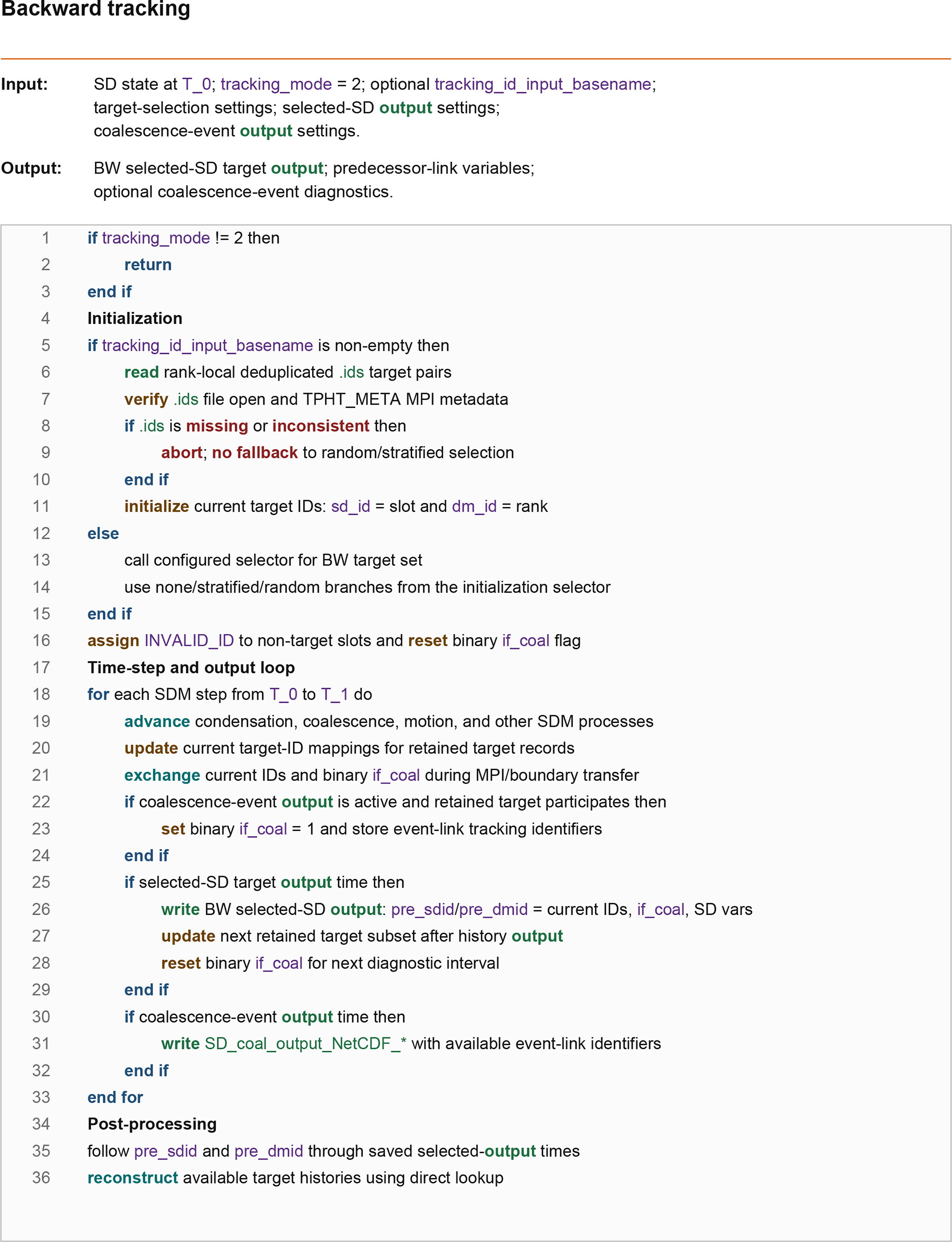
The initialisation step first defines the target subset. For each selected target super-droplet, the runtime identifier pair is initialised as “sd_id = local_index” and “dm_id = mype”, where “local_index” is the super-droplet slot within the local MPI rank and “mype” is the rank identifier. For non-target or invalid super-droplets, both identifier entries are set to “INVALID_ID”. Although the runtime arrays are stored as “sd_id/dm_id”, the backward-output writers save these values under the predecessor-link variable names “pre_sdid/pre_dmid”. Thus, in the output files, “pre_dmid” and “pre_sdid” together identify the predecessor record at the previous saved output level: pre_dmid denotes the MPI rank containing that predecessor record, and pre_sdid denotes its local record index within the corresponding rank-local output file. The predecessor-link pair is refreshed at selected-output boundaries. During an output interval, the runtime identifier pair sd_id/dm_id is propagated with each retained target. At output time t_i, the carried pair is written as pre_sdid/pre_dmid and points to the target record at the preceding saved output t_i−1. After the output is written, retained targets are remapped to their current rank and local record indices, which provide the predecessor-link values for the next output interval. The binary coalescence marker “if_coal” is initialised to zero for the selected target records and is reset to zero after each selected-super-droplet output, so that it records coalescence occurrence only within the current output interval.

At each SDM time step, the model first advances the standard super-droplet processes, including condensation/evaporation, collision-coalescence, sedimentation, advection, and MPI boundary exchange. The tracking fields are updated consistently with these processes. In particular, the current target-ID mappings are retained for target records, and both the current identifiers and if_coal are exchanged when target super-droplets cross MPI subdomain boundaries. If coalescence-event output is enabled and a retained target participates in a recorded coalescence event, if_coal is set to one for the current diagnostic interval and the available event-link tracking identifiers are stored in the coalescence-event output. At selected-output times, the model writes “SD_selected_NetCDF_^∗” files containing valid selected target super-droplet records. These records include if_coal, pre_sdid/pre_dmid, and the selected super-droplet state variables (e.g. radius, position, multiplicity and terminal velocity).

Coalescence-event output is handled through a separate event-recording pathway. When coalescence-event recording is enabled, every recorded collision-coalescence event is written to “SD_coal_output_NetCDF_^∗”. If backward tracking is active and one or both retained target super-droplets participate in the event, the event file also stores the corresponding predecessor-link identifiers, together with selected physical event variables such as radius and multiplicity. Each event record also stores the microphysics time at which the coalescence event was processed. This timestamp allows multiple recorded events involving the same target within one selected-output interval to be ordered during post-processing. Thus, if_coal provides a binary interval-level occurrence marker, whereas SD_coal_output_NetCDF_^∗ provides event-level timing and participant information. The variable if_coal in the selected super-droplet snapshot is not an event counter; it is a binary interval marker indicating whether at least one recorded coalescence event involved the target super-droplet since the previous selected-output dump. Therefore, if_coal is used in post-processing as a pointer to inspect event-log information, not as a complete collision-history record by itself.

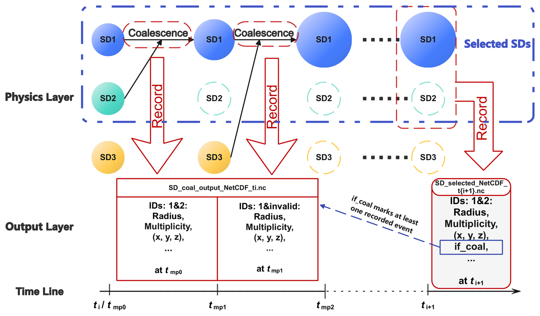
Figure 1 Schematic illustration of coalescence-event recording and selected-super-droplet output in the backward tracking algorithm. The example assumes that only SD1 and SD2 are selected target super-droplets, whereas SD3 is not selected. The times t_i and t_i+1 denote consecutive super-droplet output times, while t_mp0, t_mp1, and t_mp2 denote microphysics time steps within the same output interval. For one MPI domain and one super-droplet output interval, recorded coalescence events are appended as rows to a single SD_coal_output_NetCDF_^∗ file when coalescence-event output is enabled. Each row stores the microphysics time at which the event occurred, so multiple coalescence events involving the same selected super-droplet within the output interval can be ordered by their recorded event times. The SD_selected_NetCDF_^∗ file is written at the super-droplet output time and contains only selected target super-droplets. In forward tracking, the identifiers written to SD_selected_NetCDF_^∗ are sd_id and dm_id, which label the selected target super-droplet and the MPI rank where the target was selected. In backward tracking, the identifiers written to SD_selected_NetCDF_^∗ are pre_sdid and pre_dmid, which point to the predecessor record at the previous saved output time. When coalescence-event output is enabled, the corresponding mode-specific identifiers for recorded event participants are written to SD_coal_output_NetCDF_^∗ when available. Therefore, an unselected super-droplet such as SD3 is not written to SD_selected_NetCDF_^∗. If an unselected super-droplet coalesces with a selected target, its event-level physical information is written to SD_coal_output_NetCDF_^∗, while its tracking identifier is recorded as INVALID_ID. The variable if_coal in SD_selected_NetCDF_^∗ is a binary interval marker: it is set to 1 if at least one recorded coalescence event involving the selected target occurred between t_i and t_i+1, and remains 0 otherwise. It is not an event counter and does not by itself constitute a complete collision-history record.

Figure 1 illustrates this output structure for one selected-output interval, showing how coalescence events occurring at microphysics time steps are appended to the domain-local coalescence-event file, while selected target-super-droplet states are written only at the user-defined super-droplet output times. In the example shown in Fig. 1, only SD1 and SD2 are selected target super-droplets. An unselected event partner, such as SD3, is not written to SD_selected_NetCDF_^∗; however, if it coalesces with a selected target, its event-level physical information is written to SD_coal_output_NetCDF_^∗, while its tracking identifier is recorded as INVALID_ID. If at least one recorded coalescence event involving a selected target super-droplet occurs between two consecutive super-droplet output times, if_coal is set to 1 for that target at the later output time; otherwise, it remains 0.

The model also calculates the total number of coalescence events between the pair. Referring to the stochastic collection algorithm described in Shima et al. (2009), when the collision probability (p_α) exceeds one, it is interpreted as the expected number of collection events within the time step. A random integer (γ_α) is then generated, whose mathematical expectation equals p_α, to represent the actual number of collisions performed. Following the physical coalescence, the properties of the participating super-droplets are updated according to the model's rules. A special condition arises when both colliding super-droplets have a multiplicity of one. In this scenario, the smaller of the two is consumed and removed from the simulation, and its tracking identifiers (pre_dmid, pre_sdid) can be considered invalid for any subsequent steps, thus terminating its historical lineage. In all other cases, both parent super-droplets are preserved with updated properties. By recording the pre-collision state and the associated tracking identifiers, the event log preserves the information needed to link recorded coalescence events to the corresponding saved target histories during post-processing. The computational advantage of this design is realized during post-processing, where tracing a super-droplet's history back through time becomes a series of 𝒪(1) direct lookups, rather than an 𝒪(N) search at each step.

It is important to note, however, that the super-droplet state output used for trajectory reconstruction is written at user-defined intervals, which are generally longer than the model integration time step and microphysics time step. In our implementation, predecessor-link variables are written only at selected-output times, and coalescence-event diagnostics are written only when event output is enabled. The temporal resolution of the reconstructed target histories is therefore limited by the selected-output interval, while coalescence-event files provide additional event-level information only for recorded and linkable events. This design reduces output volume relative to writing complete target states at every microphysical time step, but it does not remove the storage and I/O dependence on output frequency and target-set size.

2.2.2 Post-Processing for Backward Tracking

The data generated by the backward tracking algorithm supports reconstruction of available saved target histories from selected output records. The post-processing workflow is designed to efficiently trace these histories from a large and distributed dataset, which is typically split by both MPI sub-domain and output time.

The process begins by identifying a set of “seed” super-droplets at a specified end time of the analysis period. These seeds are selected based on user-defined physical criteria, such as exceeding a certain radius or being located in a region of interest. Once the initial seed particles are identified, the core of the post-processing script begins tracing their histories backward in time.

For each active target record, the post-processing script reads the stored predecessor-link pair (pre_dmid, pre_sdid) and maps it to the corresponding MPI-rank file and local record index at the preceding saved output time. This operation is a direct lookup for a given key and therefore avoids a search over all super-droplets at that output time. To limit RAM use and repeated disk access, trajectories can be processed in batches and recently accessed files can be cached temporarily. The total post-processing cost, however, still depends on the number of targets, output times, variables requested, and files that must be opened.

The script repeats this lookup across saved output levels until the beginning of the available output period is reached or the predecessor-link pair becomes invalid. If if_coal = 1, the target record is marked as having participated in at least one recorded coalescence event during the preceding diagnostic interval. The post-processing workflow can then inspect the corresponding event files when event-link information is available. Because if_coal is a binary interval marker and not an event counter, this step should be interpreted as event-linked diagnostic reconstruction rather than a complete collision-history reconstruction. The reconstructed target histories are then collated into an analysis-ready output file.

2.3 Forward Tracking

2.3.1 Forward Tracking Algorithm

The forward tracking algorithm follows the subsequent evolution of selected target super-droplets by assigning persistent identifiers to them and writing their states at selected-output times. The method is summarised in Algorithm 2. In this implementation, forward tracking is activated by “tracking_mode = 1”. Selected target super-droplets are assigned the identifier pair sd_id/dm_id, where sd_id denotes the local super-droplet slot at the time of selection and dm_id denotes the MPI rank on which the target was selected. These identifiers are propagated with the super-droplet records during model integration and MPI boundary exchange. The target set is defined by the common sampling and target-selection procedure described in Sect. 2.4; therefore, the term “selected target super-droplets” is used here rather than assuming statistical representativeness for all diagnostics. The forward algorithm should therefore be interpreted primarily as an implementation and workflow component rather than as a claim of general algorithmic novelty.

Algorithm 2 A high-level representation of the forward tracking algorithm over the simulation interval [T_0, T_1], where T_0 and T_1 denote the start and end times of the tracking run or analysis window. The algorithm is activated by tracking_mode = 1, initialises a selected target subset using the common target-selection procedure, propagates sd_id/dm_id and if_coal with target super-droplet records, writes valid selected target records to SD_selected_NetCDF_^∗, and optionally records interest IDs for the two-pass hybrid workflow described later. Here, SD denotes super-droplet.

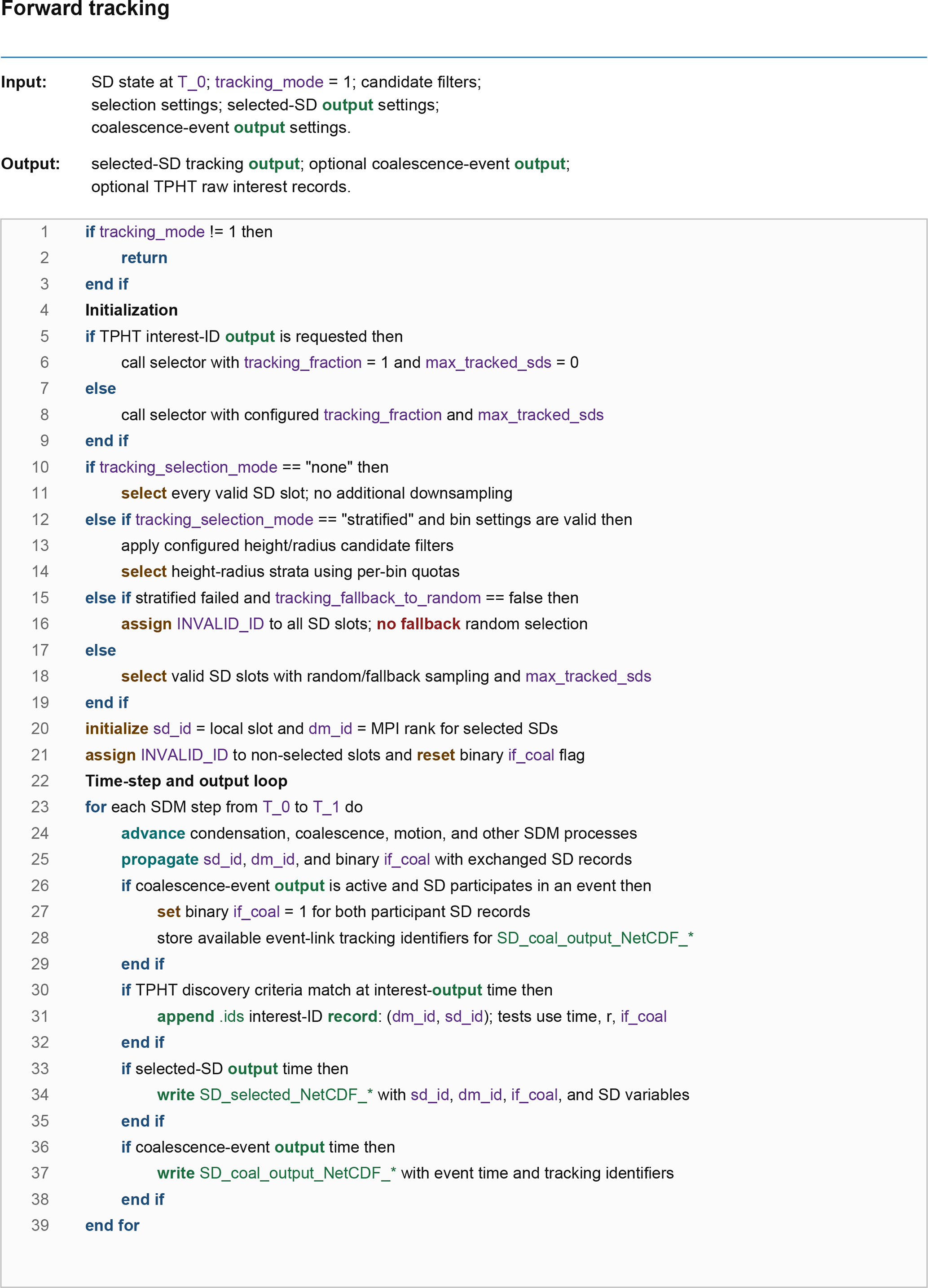
The initialisation step first defines the target subset using the configured target-selection settings. After the target subset has been determined, selected target super-droplets are initialised with “sd_id = local_index” and “dm_id = mype”, where local_index is the local super-droplet slot and mype is the MPI-rank identifier. Non-selected super-droplet slots are assigned INVALID_ID, and the binary if_coal flag is reset.

During the time-step loop, the model first advances the standard SDM processes, including condensation/evaporation, collision-coalescence, motion, sedimentation, and boundary transfer. The tracking identifiers sd_id/dm_id and the binary if_coal flag are propagated together with the corresponding super-droplet records. When selected target super-droplets cross MPI subdomain boundaries, their identifiers and if_coal values are exchanged with the super-droplet state variables, preserving target identity across the distributed-memory domain decomposition.

If coalescence-event output is active and a super-droplet participating in a recorded event has a valid tracking identifier, the algorithm sets if_coal = 1 for the corresponding participant record and stores the available event-link tracking identifiers for SD_coal_output_NetCDF_^∗. If a selected target super-droplet is removed from the simulation according to the SDM coalescence rules, its valid forward tracking record terminates and it is no longer written as a valid selected target at later output times.

At selected-output times, the model writes SD_selected_NetCDF_^∗ files containing the valid selected target super-droplet records, including sd_id, dm_id, if_coal, and the selected super-droplet state variables. Coalescence-event outputs, when enabled, are written to SD_coal_output_NetCDF_^∗ with event time and available tracking identifiers. As in the backward tracking output, if_coal is a binary interval marker and not an event counter; it indicates whether a recorded coalescence event involved the selected target during the relevant output interval.

2.3.2 Output Aggregation for Forward Tracking

The output-aggregation algorithm for forward tracking is straightforward because the selected target identifiers are written directly with each selected-super-droplet record. Analysis scripts iterate over output times and MPI-rank files, read valid records from SD_selected_NetCDF_^∗, and extract the variables needed for the diagnostic. No predecessor-link lookup is required. If a previously selected target no longer appears as a valid record at later output times, its tracked record is treated as unavailable for those times. This simple aggregation is distinct from the backward reconstruction workflow, which follows predecessor-link variables through saved output levels.

2.4 Common Target Selection and Sampling

The forward and backward tracking algorithms use the same procedure to choose which super-droplets will be saved. This procedure is called during the initialisation stage of the tracking algorithms shown in Algorithms 1 and 2. It operates on candidate super-droplets that satisfy the basic validity checks and then applies the configured sampling mode. Here we describe the ordinary target-selection modes used by the forward and backward tracking algorithms.

The simplest option is random sampling. In this mode, the candidate set consists of valid super-droplets. For each candidate super-droplet, the algorithm draws a uniform random number and retains the candidate when the draw is less than or equal to the namelist parameter “tracking_fraction”. If “max_tracked_sds” is larger than zero, selection stops when this upper limit is reached. Thus, tracking_fraction controls the expected retained fraction, while max_tracked_sds provides an optional upper bound on the number of selected target super-droplets. If tracking_fraction is less than or equal to zero, no target super-droplets are selected. If tracking_fraction is greater than or equal to one and max_tracked_sds is not set, all valid candidate super-droplets are retained.

The second option is stratified sampling. This mode first restricts the candidate population using the configured height bounds and radius bound. The remaining candidates are grouped into two-dimensional bins in height and logarithmic radius. The total target count is computed by rounding “candidate_count * tracking_fraction”, with a minimum of one target when candidates exist and “tracking_fraction > 0”, and is additionally constrained by max_tracked_sds when this cap is specified. The height coordinate is divided linearly between “tracking_height_min” and “tracking_height_max” into “tracking_nz_bin” intervals. A candidate super-droplet is assigned to a height bin according to its height within this interval. The radius coordinate is binned in logarithmic space, using “tracking_radius_min” as the lower reference radius and the largest candidate radius within the filtered population as the effective upper radius unless “tracking_radius_max” provides an active upper-bound filter. Integer bin quotas are then assigned approximately in proportion to the local candidate populations and adjusted to satisfy the total target count, with optional minimum-per-bin constraints controlled by “tracking_min_per_bin”. Within each populated bin, the retained targets are selected stochastically. Therefore, the stratified sampler should be interpreted as an approximately equal-fraction sampler over the stratified candidate population, not as an equal-count sampler from every height-radius bin. Accordingly, more populated bins receive larger quotas, while the optional tracking_min_per_bin constraint can increase the quota of populated but sparsely sampled bins when the total target budget permits. The method therefore aims to retain approximately the same fraction, rather than the same number, of candidates across bins.

If the stratified sampling path cannot be applied, for example because the bin configuration is invalid or because the configured height-radius filters produce no selected target, the behaviour is controlled by “tracking_fallback_to_random”. When this option is enabled, the algorithm falls back to the random valid-super-droplet sampling path. When it is disabled, no target super-droplets are selected for that tracking run. This rule makes the change from stratified selection to random selection explicit and user-controlled.

The selected target subset controls both the diagnostic scope and the output burden. A larger tracking_fraction increases the number of retained target records and can reduce sampling variability, but it also increases selected-output volume and post-processing cost. Conversely, a smaller tracking_fraction reduces output size but may miss rare target classes. Stratified sampling can reduce seed-to-seed variability for diagnostics that depend strongly on height or droplet size, but it does not guarantee statistical representativeness for all quantities. Representativeness depends on the sampling fraction, binning variables, target diagnostic, cloud regime, simulation duration, and output interval.

To avoid over-interpreting the selected subset, the sampling tests are treated as verification of the sampling procedure rather than as proof of general three-dimensional representativeness. A short quasi-two-dimensional sampling verification is provided in Appendix B. In that test, sampling errors decrease with increasing sampling fraction, and stratified sampling reduces seed-to-seed variability relative to purely random sampling for the tested diagnostics. These results confirm that the implemented sampling procedure behaves as intended in the tested configuration, but they should not be interpreted as a universal representativeness guarantee for all three-dimensional cloud diagnostics.

2.5 Two-Pass Hybrid Tracking

Two-pass hybrid tracking (TPHT) is a two-run method designed to reduce the amount of backward-tracking output that must be retained. In the first run, the model records the identifiers of super-droplets when they meet a prescribed radius or coalescence condition. The same identifier can be recorded many times, so an offline step removes duplicates and produces one target list. A second run starts from the same initial physical state and writes predecessor links only for the particles in this list. TPHT therefore reduces storage by giving up the ability to choose completely new targets after both runs have finished. We refer to the first integration as the discovery run, the offline removal of duplicate identifiers as ID processing, and the second integration as the reconstruction run. This target-restricted strategy is conceptually related to event- and history-based Lagrangian diagnostics used to study entrainment and mixing, in which particle histories are analysed conditionally on physically defined events or cloud-life-cycle states (Lim and Hoffmann, 2023, 2024). A full-population backward tracking configuration preserves broad freedom to choose targets after the simulation, but requires predecessor links to be written for many super-droplets and output times. TPHT trades this flexibility for lower retained output by restricting reconstruction to the predefined target list.

The workflow consists of three stages: forward discovery, offline ID processing, and backward reconstruction (Algorithm 3). The two model runs start from the same physical initial state at start time (T_0) and cover the same simulation interval to end time (T_1). In the forward-discovery stage, the model is run with tracking_mode = 1 and an output basename for interest-ID records. The tracking identifiers sd_id and dm_id are initialised and propagated with the super-droplet records. At each SDM step, the model advances the standard SDM physics and motion, updates if_coal after recorded coalescence participation, and tests the user-defined interest criteria. In the present implementation, these criteria can include radius-threshold exceedance or a binary coalescence-participation condition. When a target satisfies the interest criteria, the model appends an interest-ID record containing the pair dm_id and sd_id. The resulting per-rank “.ids” files are raw interest-ID streams used by the offline processing stage; they are not the target list supplied directly to the second run and contain no physical restart state. These files contain the tracking-ID pair together with decomposition metadata, but not super-droplet physical states. Additional event-level diagnostics, such as event time and partner radii, are written separately to SD_coal_output_NetCDF_^∗ when coalescence-event logging is enabled; these diagnostics are used as event records rather than as a complete process budget.

Algorithm 3 High-level representation of two-pass hybrid tracking (TPHT) over the simulation interval [T_0, T_1], where T_0 and T_1 denote the start and end times of the tracking run or analysis window. TPHT first performs a forward-discovery run to append interest-ID records for super-droplets satisfying predefined radius- or coalescence-based criteria. The raw rank-local ID streams are then merged, checked for MPI-decomposition consistency, deduplicated by dm_id and sd_id, and repartitioned into target-list files. A second run starts again from the same physical initial state at T_0, reads the deduplicated target-ID files before ordinary sampling, and performs backward reconstruction only for this target set. The .ids files are target-list files, not physical restart files. SD, FW and BW are abbreviations for super-droplet, forward and backward, respectively.

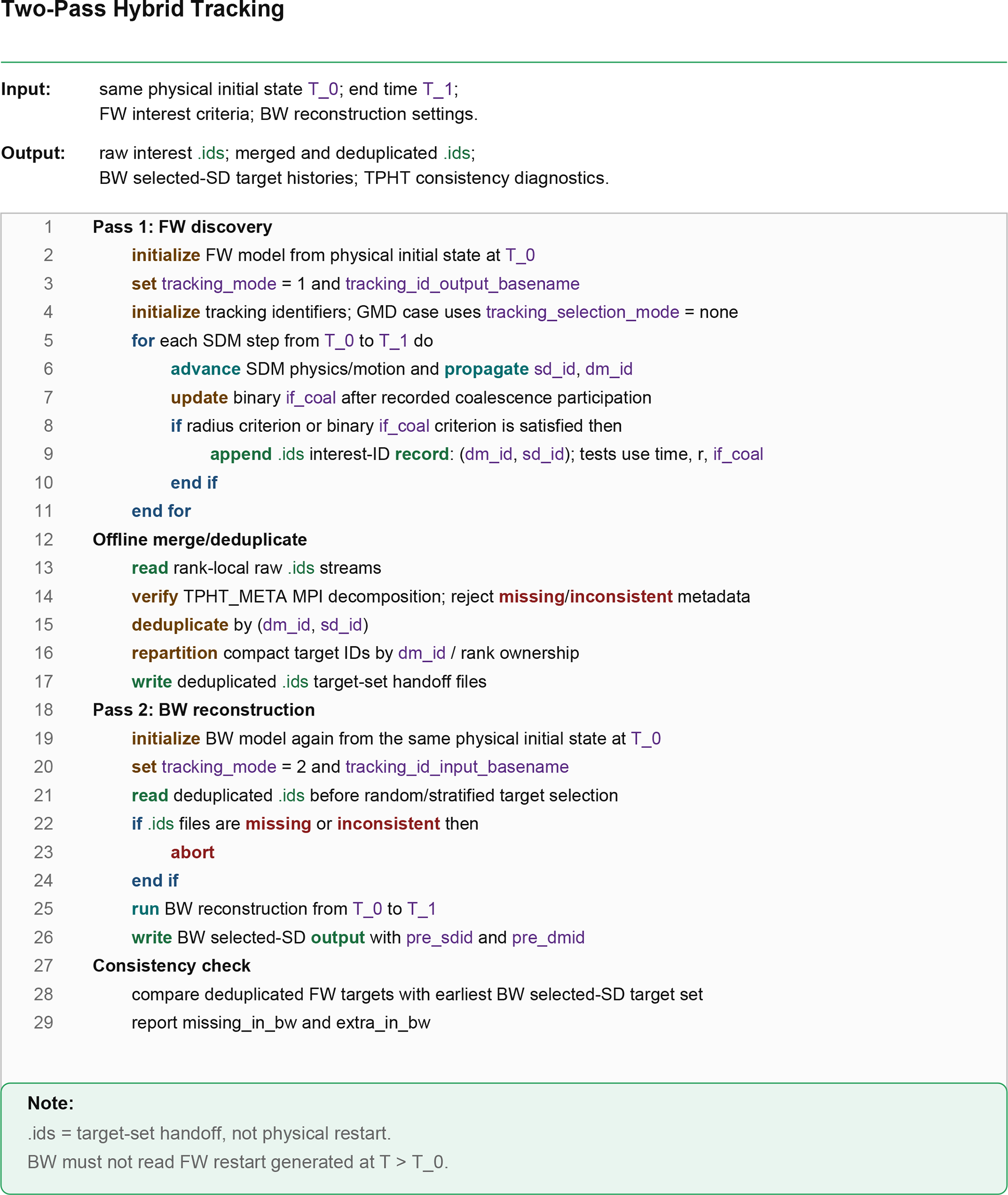
The raw interest-ID records are then processed offline. Rank-local streams are read, their MPI-decomposition metadata are checked, and records with missing or inconsistent metadata are rejected. The remaining records are deduplicated by the pair dm_id and sd_id, because the same super-droplet can satisfy the interest criteria at multiple times. The deduplicated target IDs are then repartitioned according to rank ownership and written as compact target-list files. These files define the target set for the following backward-reconstruction run. They are not physical restart files; they contain target identifiers used for reconstruction and do not replace the physical initial state of the simulation.

In the backward-reconstruction stage, the model is initialised again from the same physical initial state at T_0. The run is performed with tracking_mode = 2 and reads the deduplicated target-list files before any ordinary random or stratified target selection is applied; in TPHT, this external target set takes priority over ordinary sampling. If the required target-list files are missing or inconsistent, the run aborts rather than silently falling back to another target-selection mode. The model then evolves from T_0 to T_1 and writes selected-super-droplet output for the deduplicated target set, including the predecessor-link variables pre_sdid and pre_dmid. These output files are subsequently used to reconstruct the available target histories by direct lookup.

A consistency check is performed after the backward-reconstruction run. The deduplicated target set from the forward-discovery stage is compared with the earliest selected-super-droplet target set written by the backward-reconstruction stage. The diagnostics “missing_in_bw” and “extra_in_bw” report whether any discovered targets were not reconstructed or whether any additional targets appeared in the reconstruction output. This check verifies the target list between the two passes, but it does not imply that TPHT provides arbitrary access to every super-droplet history. This check establishes complete transfer of the target-ID list only; it does not by itself establish equality of the physical histories generated by the two integrations. The available physical-event comparison is reported separately in Sect. 3.2.4. This consistency check is meaningful only because the backward-reconstruction pass starts from the same TPHT initial physical state as the forward-discovery pass. TPHT remains an interest-restricted workflow whose usefulness depends on the chosen target criteria.

Across the tracking workflows, the main output files have distinct roles. Forward tracking writes selected target states and persistent identifiers sd_id and dm_id to SD_selected_NetCDF_^∗. Backward tracking writes selected target states and predecessor-link identifiers pre_sdid and pre_dmid to SD_selected_NetCDF_^∗. Coalescence-event diagnostics, when enabled, are written separately to SD_coal_output_NetCDF_^∗. TPHT forward discovery writes raw .ids interest-ID streams, and the offline merge step writes deduplicated per-rank .ids target-list files for the backward-reconstruction pass. For selected-super-droplet output, one NetCDF file is written per MPI rank and selected-output time; coalescence-event files are grouped by event-output bucket and rank and are written only when recorded events exist.

For the two integrations to follow the same stochastic realisation, they must use the same source and executable, compiler and floating-point settings, numerical libraries, MPI rank count and decomposition, effective thread count, initial physical and physical random-number states, floating-point operation ordering, and physical random-number call order. Tracking selection uses a separate random-number generator, and the audited identifier, output, and boundary-exchange paths do not alter the physical super-droplet arrays or collision-pair construction. These are requirements for simulation-level reproducibility. The separate code-level checks of target-ID transfer and recorded coalescence history are described in Sect. 3.2.4, and broader numerical limitations are discussed in Sect. 4.2.

2.6 Practical Comparison of Tracking Workflows

The three tracking workflows differ primarily in when and how the target super-droplets are defined. Backward tracking is useful when targets are identified after the simulation has evolved, forward tracking is useful when targets can be selected before or during the simulation, and TPHT is useful when targets are defined by event- or threshold-based interest conditions discovered during a preceding tracking run. These workflows should therefore be viewed as complementary selected-target diagnostics rather than as universally interchangeable alternatives.

Backward tracking is most appropriate for a posteriori diagnostic in which target particles are identified after the simulation has evolved. Examples include droplets that exceed a specified radius, particles located in a specified cloud region, or super-droplets that participate in recorded coalescence events. Its main advantage is that the target class does not need to be fixed at initialisation. Its main limitation is that the required predecessor-link information must already have been written; therefore, storage and I/O can become limiting when many particles, variables, or output times are retained.

The event- and history-conditioned perspective adopted in this study was particularly inspired by Lim and Hoffmann (2023, 2024), who analysed particle histories conditional on entrainment and mixing events. Other previously studied problems illustrate potential applications of backward tracking, including lucky-droplet and stochastic-growth analyses (Telford, 1955; Hoffmann et al., 2017; Dziekan and Pawlowska, 2017; Li et al., 2022), eddy hopping (Cooper, 1989; Grabowski and Abade, 2017; Abade et al., 2018), and droplet-spectrum broadening associated with mixing (Baker et al., 1980; Burnet and Brenguier, 2007). These studies are cited as examples of scientific questions that may benefit from a posteriori particle-history reconstruction; they are not analysed in the present case study.

Table 1 Practical comparison of the tracking workflows.

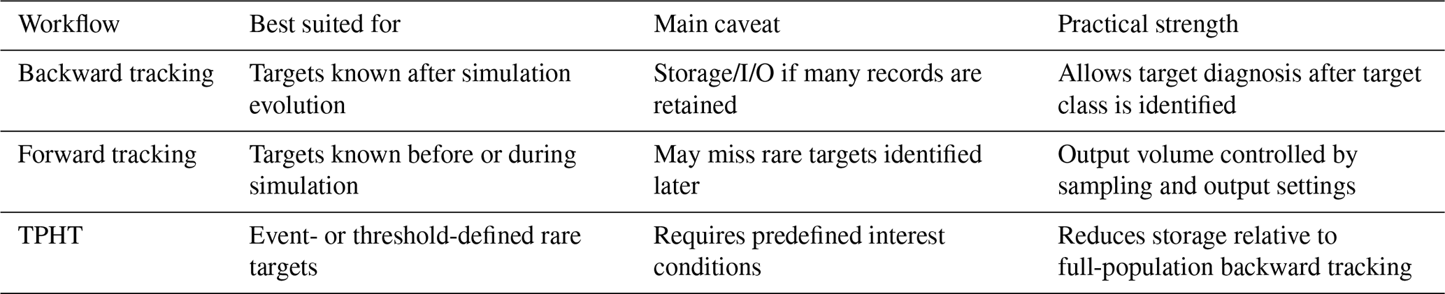
The storage cost of backward tracking depends on the size of the retained target set and the output frequency. Saving backward links for the full particle population leaves many possible targets available for later analysis, but also maximises the amount of predecessor-link output. A target-restricted configuration reduces this burden by retaining only a physically defined subset, at the cost of losing arbitrary access to unretained super-droplet histories. This distinction is central for three-dimensional applications: the direct lookup used during reconstruction reduces search complexity, but it does not remove the need to write the predecessor-link information that will later be queried.

Forward tracking is most useful when the target set can be defined before or during the simulation. The selected target super-droplets are assigned persistent identifiers and their subsequent states are written directly to selected-output files. Its main practical advantage is that output volume can be controlled by the sampling fraction, target filters, output interval, and variable selection. It is therefore suitable for experiments in which the particles of interest are known a priori, such as prescribed target cohorts, sensitivity experiments, or externally introduced particles.

The main limitation of forward tracking is that target selection is partly a priori. If a rare target class is only identifiable after the simulation has evolved, a fixed initial sample may miss some relevant particles unless the sampling fraction or target criteria are chosen accordingly. In addition, the sampled subset should not automatically be interpreted as statistically representative for all diagnostics. Representativeness depends on the sampling mode, sampling fraction, stratification variables, cloud regime, simulation duration, and diagnostic quantity. For this reason, forward tracking is best described as selected-target output, with representativeness assessed separately for the diagnostic of interest. The post-processing step for forward tracking is usually a direct aggregation of selected-output records across output times and MPI-rank files. Its cost is therefore mainly controlled by the number of selected records and files to be read, rather than by a lineage-reconstruction lookup. Simply increasing the number of particles retained by forward tracking is not equivalent to TPHT. Forward tracking remains an a priori selected-output strategy: it writes full selected-output histories for particles chosen before or during the simulation. Increasing the sampling fraction can reduce the chance of missing rare targets, but the output volume scales with the number of retained particles, output times, and variables written. In the limit, using forward tracking to guarantee capture of all rare a posteriori targets approaches a full-population selected-output problem. TPHT avoids writing full histories for a large forward sample. The first run saves only identifiers when a particle meets the chosen condition; the second run then writes histories only for the resulting unique targets.

The TPHT workflow is designed for cases in which the target class is not known at initialisation but can be defined by event- or threshold-based conditions during the simulation. A forward discovery run identifies candidate target IDs, and a subsequent backward reconstruction run follows only the deduplicated target set. This approach reduces the storage burden relative to full-population backward tracking, while avoiding the purely a priori limitation of ordinary forward tracking. Its limitation is that the target class must be specified through predefined interest conditions; it does not provide unrestricted access to every super-droplet history after the fact.

Table 1 summarises the main use case and primary caveat of each workflow.

3 Application and Results: A Stratocumulus Case Study

The purpose of this section is to demonstrate the TPHT workflow in a stratocumulus simulation, rather than to establish a new general mechanism of warm-rain formation.

3.1 Case Description

The case study employed in this research is the second research flight of the second Dynamics and Chemistry of Marine Stratocumulus field campaign (DYCOMS-II RF02) (Stevens et al., 2003). This case, part of the international DYCOMS project, is based on observations of nocturnal marine stratocumulus off the coast of Southern California on 11 July 2001. It is characterised by a bimodal cloud field, containing regions of closed-cell stratocumulus with light drizzle, interspersed with open-cell areas producing stronger precipitation. The initial thermodynamic conditions represent an average state of these two cloud regimes, while the microphysical conditions are representative of the open-cell regions. Due to its idealized boundary conditions, initial fields, and the availability of rich observational data, the DYCOMS-II RF02 case has been widely used for the evaluation and validation of cloud models, particularly for LES.

3.2 Simulation Setup

3.2.1 General Model Configuration

All simulations were performed using the SCALE-SDM model, which solves the compressible Navier-Stokes equations for moist air using a finite-volume method with a forward-in-time integration scheme. The spatial discretization of Eulerian variables is performed on an Arakawa-C staggered grid (Arakawa and Lamb, 1977). A fourth-order central difference scheme is used for the advection of prognostic dynamical variables, while a third-order upwind scheme by Koren (1993) is used for tracer advection. Other spatial derivatives are approximated using a second-order central difference scheme. For time integration, a fourth-order Runge–Kutta scheme is applied to dynamical variables, and a third-order Runge–Kutta scheme by Wicker and Skamarock (2002) is used for tracers. SGS turbulence is parameterised using a Smagorinsky–Lilly type scheme (Lilly, 1962; Smagorinsky, 1963), which includes stratification effects. To ensure numerical stability, fourth-order hyper-diffusion is added, with the dimensionless coefficient set to 10⁻⁴ as defined in Nishizawa et al. (2015).

SDM explicitly calculates the temporal evolution of aerosol, cloud, and precipitation particles. The microphysical processes considered in this study include advection, sedimentation, evaporation/condensation (including activation/deactivation of cloud condensation nuclei), and, in some simulations, collision-coalescence. To handle the stiffness problem, the condensation/evaporation process is solved using an implicit Euler scheme. The coalescence process is handled by the Monte Carlo stochastic algorithm of Shima et al. (2009). Super-droplets are initialised using a uniform sampling method (see Sect. 5.3 of Shima et al., 2020). The interaction between super-droplets and SGS turbulence is not directly considered in the current version of the model. For more details on the governing equations and numerical schemes, refer to the works of Shima et al. (2009, 2020).

The initial vertical profiles for wind, humidity, and temperature follow the setup of Ackerman et al. (2009), with doubly periodic lateral boundary conditions. A simplified radiation model as described in Ackerman et al. (2009) is used. Following Ackerman et al. (2009), supersaturation was capped at 1 % during the first hour of simulation. They adopted this constraint to prevent excessive activation of Aitken-mode particles during the initial spin-up, which could otherwise hinder precipitation development compared to simulations with fixed droplet number concentrations. The initial aerosol population follows the bimodal lognormal distribution specified in Ackerman et al. (2009). Constant surface sensible and latent heat fluxes are considered, with the latter slightly reduced from 93 to 86.7132 W m⁻² to prevent overestimation of the liquid water content. Momentum exchange between super-droplets and the fluid is also taken into account (see Shima et al., 2009, 2020 for detailed information).

3.2.2 TPHT Experiment Setups

To demonstrate TPHT as a practical three-dimensional backward-reconstruction workflow, an experiment was performed using the DYCOMS-II RF02 configuration and an SDNC (super-droplet number concentration) of 40 per cell. The domain was set to 2 km × 2 km × 1.5 km with a grid resolution of 50 m × 50 m × 5 m, corresponding to a 40 × 40 × 300 grid. The model was integrated for 70 min in the full three-dimensional domain; the first 60 min were treated as spin-up. TPHT was implemented as two model integrations over the same physical time interval, both initialised from the same physical and random-number state.

In the first integration, the forward discovery pass was run with tracking_mode = 1. No random or stratified downsampling was applied during the initial tracking-ID assignment; instead, the backward target set was reduced by interest criteria evaluated during the forward run. A super-droplet was added to the rank-local target-ID stream when its radius reached 15 µm or when the binary coalescence flag if_coal indicated participation in at least one recorded coalescence event within the current selected-output interval. During this discovery pass, ordinary Eulerian history output and selected super-droplet trajectory output were suppressed, and rank-local .ids streams were written for offline processing.

The rank-local target-ID streams were then merged and deduplicated by the tracking-identifier pair (dm_id, sd_id), with metadata checks for consistency of the MPI decomposition. The resulting deduplicated .ids files were supplied to the second integration through the namelist key “tracking_id_input_basename”, which specifies the basename of the external target-ID list read by the backward-reconstruction run. This backward reconstruction pass was run with tracking_mode = 2 and was initialised again from the same physical state at the beginning of the TPHT interval, rather than from a restart produced by the forward discovery pass. It wrote selected target states to SD_selected_NetCDF_^∗ every 10 s, and Eulerian history fields were written at the same interval. Coalescence-event logging was also enabled, producing SD_coal_output_NetCDF_^∗ diagnostics for recorded event-level information between saved selected-output times. Thus, the .ids files serve only as a target list, not as a physical restart. This setup restricts the expensive backward reconstruction to interest-defined targets while retaining available predecessor-link histories for the selected target set.

Table 2 Configuration of the two model integrations used in the TPHT experiment. The forward-discovery pass writes raw per-rank “.ids” interest-ID streams, whereas the backward-reconstruction pass starts again from the same initial physical and random-number state and reads deduplicated per-rank .ids target-set files. The .ids files are target-list files, not physical restart files. Coalescence-event logging is enabled in both passes, and recorded events are appended to 10 s file buckets only when events occur.

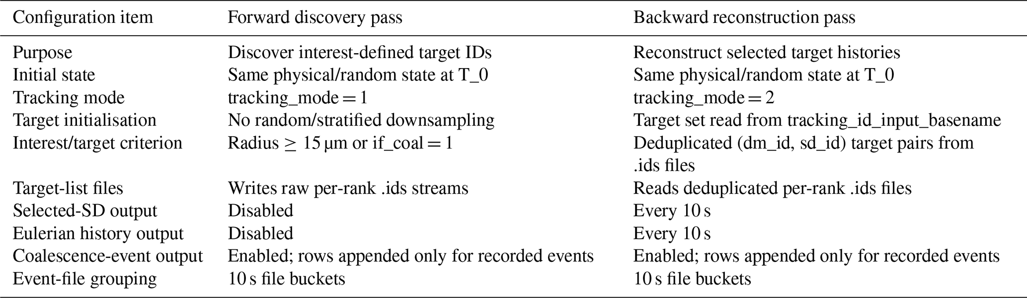
The key configuration differences between the forward-discovery and backward-reconstruction passes are summarised in Table 2.

3.2.3 Computational and Storage Characteristics

The simulations were performed on the general-purpose CPU nodes of the Osaka University D3 Center SQUID system. Each CPU node has two Intel Xeon Platinum 8368 processors (Ice Lake, 2.40 GHz, 38 cores per processor; 76 cores per node), 256 GB of RAM, and Mellanox InfiniBand HDR interconnects at 200 Gbps. The three-dimensional jobs generally used 64 MPI ranks. The model was compiled with the Intel Fortran compiler 2023.2.4 and Intel MPI 2021.11 (Build 20231005), using mpiifort invoking ifort. The linked threading and math libraries were oneTBB 2021.10.0 and MKL 2023.2.0. Parallel I/O used HDF5 1.12.3 with MPI support, netCDF-C 4.9.2, and netCDF-Fortran 4.6.1.

The controlled three-dimensional benchmark is summarised in Appendix A and Fig. A1. In this benchmark, the 5 % sampled forward and backward tracking configurations showed no large wall-clock or peak-RAM penalty relative to the no-tracking baseline. The wall-clock times were 8750–8754 s for the sampled tracking configurations and 8982 s for the no-tracking baseline, while peak RAM per rank remained around 649–653 MiB compared with 650 MiB for the baseline. The main additional burden was output volume: the sampled tracking cases wrote about 121 MiB of diagnostic output, whereas the no-tracking baseline wrote no selected-super-droplet output. The coalescence-log-only case wrote about 4.37 MiB of coalescence-event diagnostics.

Additional sensitivity tests are also reported in Appendix C. The SDNC-scaling test shows that wall-clock time increased with SDNC over the tested range, with empirical log-log slopes of about 0.78–0.83 for the no-tracking and 5 % sampled tracking cases. The number of tracked chains scaled approximately linearly with SDNC, whereas peak RAM increased only weakly. The output-interval test shows that selected-super-droplet output volume decreased as the output interval increased. Because each output operation then contained more records, the mean write time per output operation increased, although the total write-time response depended on the tracking configuration. A short quasi-two-dimensional sampling-procedure verification is provided separately in Appendix B and Fig. B1. That test verifies the sampling workflow and quantifies seed-to-seed variability in a short two-dimensional setup; it is not used as evidence for long-time three-dimensional representativeness.

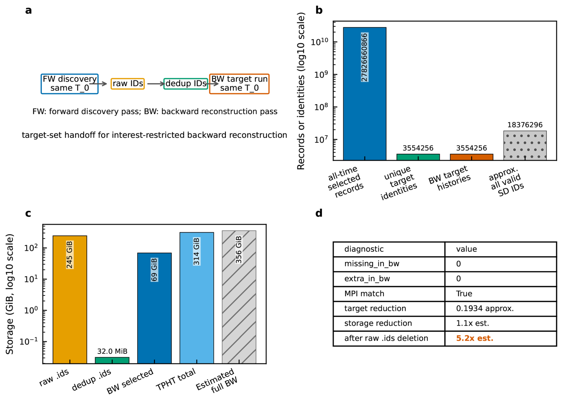
Figure 2 TPHT target transfer and storage diagnostics. (a) Schematic of the TPHT workflow: FW discovery identifies interest-defined target IDs, offline processing deduplicates the target set, and BW reconstruction follows the deduplicated targets from the same initial physical state. (b) Number of all-time discovery records, deduplicated target identities, BW-reconstructed target histories, and estimated valid super-droplet IDs. (c) Storage volumes for raw ID streams, deduplicated target list, BW selected output, total TPHT working storage, retained TPHT storage after raw-ID deletion, and estimated full-population BW output. (d) Target-list diagnostics showing that all deduplicated targets were recovered in BW reconstruction, with no additional reconstructed targets and consistent MPI-rank ownership. FW and BW denote forward and backward tracking, respectively. Estimated full-population BW output is used for the storage-reduction estimates.

The TPHT storage and target-list diagnostics are summarised in Fig. 2. The forward-discovery pass generated 27 826 660 866 all-time interest-ID records. These records include repeated detections because the same super-droplet can satisfy the interest criteria at multiple times. Offline deduplication reduced this stream to 3 554 256 unique target identities. The target-list check showed that all deduplicated targets were recovered in the backward-reconstruction output, with no additional reconstructed targets, and the MPI-decomposition consistency check was true. These diagnostics indicate that the target list between the forward-discovery pass and the backward-reconstruction pass was internally consistent.

The deduplicated target set contained 3 554 256 identities. Let ${\mathit{\varphi }}_{\text{tgt}}=N_{\text{target}}/N_{\text{full}}$ denote the retained-target fraction, where N_full is the estimated number of valid super-droplet identities; here, ϕ_tgt≈ 0.193. Assuming that backward selected-output size scales approximately with the number of retained identities under otherwise unchanged output settings, the estimated retained-storage reduction after deleting the temporary raw identifier files is R_storage≈ 1$/{\mathit{\varphi }}_{\text{tgt}}\approx$ 5.2. The factor is specific to the relatively broad radius and coalescence criteria used in this demonstration and is not an upper limit of TPHT. Sparser target definitions could yield substantially larger reductions.

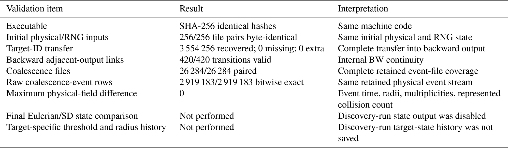
Table 3 Summary of TPHT target-ID transfer and coalescence-history verification. The event-row count refers to the complete raw coalescence-event logs from the two passes. Figure 3b uses a separately derived target-linked subset. “Not performed” denotes comparisons that could not be made because the forward-discovery run did not save Eulerian or selected-super-droplet state histories. RNG denotes random-number generator.

The raw interest-ID streams occupied 245 GiB. These raw streams are intermediate working files used for offline merging and deduplication. After deduplication, the compact per-rank target-list files occupied only 32.0 MiB. Thus, the deduplicated target list itself is small, even though the all-time discovery stream is large. The backward-reconstruction pass wrote 69 GiB of selected target output. If all raw discovery streams are retained, the total TPHT working storage is 314 GiB, compared with an estimated 356 GiB for full-population backward output, corresponding to an estimated end-to-end storage reduction of about 1.1×. However, the raw interest-ID streams can be deleted after the deduplicated target-list files have been generated. After this cleanup, the retained TPHT storage is dominated by the 69 GiB backward selected output plus the 32.0 MiB target list, corresponding to an effective retained-output reduction of about 5.2× relative to the estimated full-population backward output. The use of raw interest-ID streams is a deliberate design choice. The forward-discovery pass may encounter a very large number of interest-condition hits when the selected target class is broad or when the simulation contains many time steps. Deduplicating these hits inside the model, or keeping a large in-memory set of all previously detected IDs until the end of the run, would add runtime overhead and increase RAM use during the SDM integration. TPHT instead writes raw interest-ID records sequentially and transfers the deduplication step to offline post-processing. This design trades temporary working storage for lower in-model bookkeeping cost. In the present analysis, the offline merge/deduplication step was not recorded as a separate wall-clock metric; therefore, only the resulting file sizes are reported here. The lack of a separately instrumented merge/deduplication wall-clock time is a limitation of the present benchmark. The TPHT storage numbers therefore quantify the model-output and retained-analysis burden, whereas the total end-to-end workflow cost additionally includes offline parsing, deduplication, repartitioning, and target-list writing. In future benchmark runs, these offline stages should be timed separately. In the present manuscript, TPHT should therefore be interpreted as a storage- and diagnostic-workflow demonstration rather than as a complete end-to-end performance optimum.

The backward reconstruction itself uses direct lookup once the predecessor-link pair is known, so each predecessor query avoids a search over all super-droplet records at a given output time. This 𝒪(1) lookup property applies to a single predecessor query, not to the complete workflow; the total post-processing cost still depends on the number of reconstructed targets, saved output times, variables read, and file I/O. Overall, these results demonstrate that TPHT can perform a consistent three-dimensional interest-restricted backward reconstruction while separating temporary discovery output from retained reconstruction output. The storage benefit depends on the sparsity of the interest criteria, the selected-output interval, the variables written, and whether raw discovery streams are retained after deduplication. TPHT should therefore be interpreted as a practical target-restricted workflow rather than as eliminating the storage cost of full-population backward tracking in all configurations.

3.2.4 TPHT Target-ID Transfer and Coalescence-History Verification

Two different checks are considered here. A common practical check of simulation-level reproducibility is to compare Eulerian output from two model integrations. The forward-discovery run did not save Eulerian history or selected-super-droplet state output because these outputs were disabled to reduce storage, so this comparison could not be made from the archived files. The present analysis instead addresses two code-level questions specific to TPHT: whether the target-ID list was transferred completely to the backward-reconstruction run, and whether the second run recorded the same physical coalescence history as the first run.

We first compared the executable and four sets of rank-local input files used by both integrations: boundary files, DYCOMS initial-state files, physical random-number-state files, and reference-state files. We then read all corresponding coalescence-event files sequentially. Because the warm-cloud event files contain no global event identifier, records were paired by the same rank/time-bucket filename and ordered event-row index. Event time, both pre-update radii, both multiplicities, and the represented collision count were compared bitwise. Forward and backward tracking identifiers were analysed separately because they have different meanings. Table 3 summarises the target-ID transfer and coalescence-history checks.

The executable used by both integrations had the same SHA-256 hash, and all 256 corresponding input-file pairs were byte-identical. The target-list files contained 3 554 256 unique identities, all of which were recovered in the backward output without additional targets. The event-log audit compared all 26 284 corresponding file pairs and 2 919 183 event rows in each run. Every row agreed bitwise in event time, both pre-update radii, both multiplicities, and the represented collision count, with a maximum difference of zero for every compared field. The exact agreement of these event records provides evidence that the two integrations reproduced the same recorded coalescence history under the tested configuration. This is a code-level verification of TPHT rather than a comparison of every model-state variable.

Figure 3 Comparison between the Hall gravitational collection kernel and TPHT-diagnosed coalescence-record radius pairs. (a) Hall kernel as a function of droplet radii R_j and R_k (µm). The colour scale shows the collection kernel, including collection efficiency, geometric sweep-out area, and differential terminal fall speed; it is therefore not a dimensionless coalescence probability. (b) Radius-pair distribution from the derived TPHT target-linked event table, containing 2 919 104 two-participant coalescence records. The two participant radii are sorted into larger and smaller radii and accumulated in logarithmic bins. The colour scale shows the normalised multiplicity-weighted frequency of realised SDM coalescence records linked to TPHT targets. Both panels use logarithmic axes and the same radius range.

The raw-log population is distinct from the derived target-linked table used in Fig. 3b. The latter contains 2 919 104 two-participant coalescence records after applying the output-window and backward-chain-linkage requirements described in Sect. 3.3. The forward-discovery run did not save Eulerian history or selected-super-droplet state histories. Complete later model states, the time of the first r≥ 15 µm threshold crossing, and the preceding radius evolution therefore could not be compared from the archived files.

3.3 Coalescence-Event Context for TPHT Target Selection

In the current version of SCALE-SDM, droplet growth by coalescence considers only gravitational collection; the effects of turbulence on coalescence are not yet included. To understand the simulation results, we first consider the fundamental physics governing this process. The coalescence probability, P_jk, between two real droplets (j,k) within a volume ΔV over a microphysical time step dt_mp is determined by their physical properties (Shima et al., 2009, 2020):

$$\begin{array}{}\text{(1)}& P_{jk}=E_{\text{coal}}(R_j,R_k)\mathit{\pi }(R_j+R_k{)}^{\mathrm{2}}\mathrm{|}{v}_j^{\mathrm{\infty }}-v_k^{\mathrm{\infty }}\mathrm{|}\text{dt}\mathit{\_}\text{mp}/\mathrm{\Delta }V\end{array}$$

where R represents the radius, v^∞ is the terminal fall velocity, and E_coal is the collection efficiency. In this study, the collection efficiency is calculated using the Hall's kernel (Hall, 1980) as modified by Seeßelberg et al. (1996) and Bott (1998). Since each super-droplet represents a multiplicity of real droplets with identical radii and velocities, P_jk directly dictates the likelihood of coalescence events in the SDM algorithm. The collection efficiency itself is dimensionless and depends on the radii of the interacting droplets. In contrast, the gravitational collection kernel used below combines this efficiency with the geometric sweep-out area and the differential terminal fall speed. The kernel therefore emphasizes radius pairs for which gravitational collection is expected to be efficient, particularly when one or both droplets are sufficiently large and the differential fall speed becomes appreciable.

Figure 3 compares this theoretical radius-pair dependence with the coalescence-event records linked to the TPHT target set. Figure 3a provides a reference map of the Hall gravitational collection kernel in radius-pair space. The plotted quantity is not the dimensionless collection efficiency alone, but the radius-dependent collection kernel, which combines Hall's collection efficiency with the geometric sweep-out area and the differential terminal fall speed. It is therefore used as a physical reference for interpreting which droplet-size combinations are expected to contribute efficiently to gravitational collection.

Figure 3b shows the radius-pair distribution represented in the derived TPHT target-linked event table. The plotted distribution aggregates the linked coalescence records over all available model output times in the TPHT reconstruction period, rather than representing a single output snapshot. For each linked coalescence record, the two pre-coalescence super-droplet radii are sorted into larger and smaller radii and accumulated in logarithmic radius bins. The distribution is shown as a normalised multiplicity-weighted frequency, so the panel characterises which radius pairs dominate the represented real-droplet coalescence population in the TPHT-linked event records. The panel contains 2 919 104 two-participant coalescence records constructed from the backward-run event logs after applying the output-window and chain-linkage requirements. It is therefore a linked subset of the 2 919 183 raw event records compared in Sect. 3.2.4.

Figure 4 Characteristics of super-droplets selected by the TPHT criteria. (a) Target classification by the first recovered interest condition. Targets without an if_coal-marked selected output are grouped with the radius-threshold class, because they correspond to targets selected by radius-threshold exceedance. (b) Height distribution of the first recovered r≥ 15 µm crossing, with bins chosen to highlight the mean cloud-layer range of approximately 400–800 m. (c) Median radius at first r≥ 15 µm crossing and median maximum reconstructed radius; the dashed line marks the 15 µm threshold. All statistics include the spin-up period and are used as target-set diagnostics.

The purpose of this comparison is contextual. Figure 3a shows where the gravitational collection kernel is large in radius-pair space, whereas Fig. 3b shows which pre-coalescence radius pairs appear frequently in the realised SDM coalescence records linked to TPHT targets after multiplicity weighting. Differences between the two panels should not be interpreted as a validation of the Hall kernel or as a closed collision–coalescence budget. The recorded distribution depends on the simulated droplet population, multiplicities, local collision opportunities, stochastic collection sampling, the microphysics time step, and the event-recording configuration. The comparison is therefore used as radius-pair context for the coalescence-participation criterion in TPHT.

3.4 Characteristics of the Selected TPHT Target

The TPHT target diagnostics characterise the selected target set reconstructed in the three-dimensional demonstration. Figure 4 summarises the recovered target classes and radius-threshold diagnostics. The deduplicated target set contained 3 554 256 targets, including 2 279 068 targets that reached the radius threshold and 1 676 150 targets that carried the if_coal flag at least once. The radius-threshold condition accounts for the largest class of targets, while smaller fractions are associated with the if_coal flag or with both diagnostics. In this classification, targets without an if_coal-marked selected output are included in the radius-threshold class, because they correspond to targets selected by radius-threshold exceedance; some of these targets may have exceeded 15 µm between selected-output times and then evaporated below the threshold before the next saved output.

For targets that crossed the radius threshold, the first recovered r≥ 15 µm crossings were concentrated mainly in the 600–800 m height range, corresponding approximately to the upper part of the mean cloud layer, which was about 400–800 m in this simulation. The median radius at first threshold crossing was close to 15 µm, and the median maximum reconstructed radius remained only slightly above this value. This indicates that many selected targets were near-threshold droplets rather than substantially larger drops.

These statistics are computed over the full simulated period, including the cold-start spin-up stage. They are therefore used here as a TPHT diagnostic characterisation of the reconstructed target set.

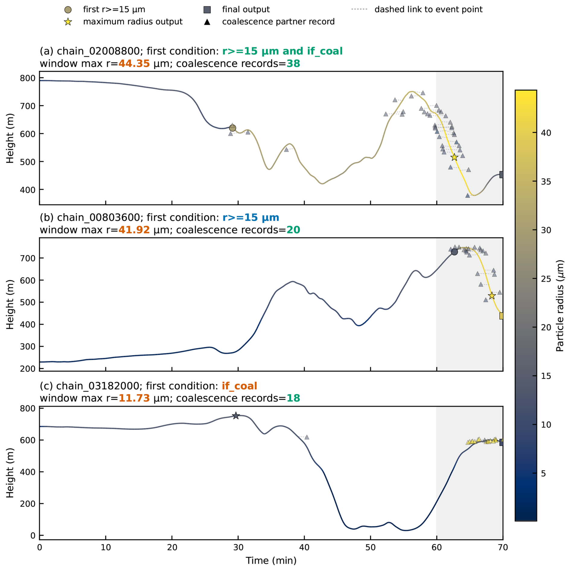
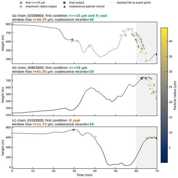
Figure 5 Example super-droplet histories reconstructed with TPHT for three selected targets in the final 10 min of the 70 min TPHT demonstration. The three panels show cases whose first recovered target-selection condition was (a) both r≥ 15 µm and if_coal, (b) r≥ 15 µm only, and (c) if_coal only. Lines show reconstructed target height versus model time, coloured by target super-droplet radius. Circles mark the first output at which r≥ 15 µm, stars mark the maximum-radius output, and squares mark the final output at which the target remained a valid selected super-droplet. Triangles mark target-linked coalescence records from SD_coal_output_NetCDF_^∗, with triangle colour indicating the radius of the coalescence partner. To avoid obscuring the target trajectory, the triangles are plotted in nearby blank regions and connected to the corresponding event locations by dashed guide lines. The grey shading denotes the final 10 min selection window. Text annotations give the first recovered selection condition, the maximum radius within the final 10 min window, and the number of linked coalescence records over the reconstructed history. The plotted coalescence records are diagnostic event-log links rather than a complete causal process budget.

3.5 Examples of Super-Droplet Histories Reconstructed with TPHT

To illustrate what information can be recovered for individual TPHT-selected targets, Fig. 5 shows three predecessor-chain examples selected from the final 10 min of the 70 min TPHT demonstration. The grey shading in each panel marks this final 10 min selection window, but the reconstructed histories include the available target records and target-linked coalescence records over the full simulation period. The examples span the three first recovered target-selection conditions used in the target diagnostics: simultaneous radius-threshold and coalescence-flag selection, radius-threshold-only selection, and coalescence-flag-only selection.

The curves show target height as a function of model time, with line colour indicating the target super-droplet radius. Circles mark the first output at which the target reached (r≥ 15 µm), stars mark the maximum-radius output, and squares mark the final output at which the target remained a valid selected super-droplet. Target-linked coalescence records are indicated by triangles. To avoid obscuring the target trajectory, the triangles are placed in nearby blank regions of the panel, and dashed guide lines point to the corresponding event locations on the reconstructed trajectory. The triangle colour indicates the radius of the coalescence partner. Each panel also reports the first recovered selection condition, the maximum radius within the final 10 min selection window, and the number of linked coalescence records over the reconstructed history.

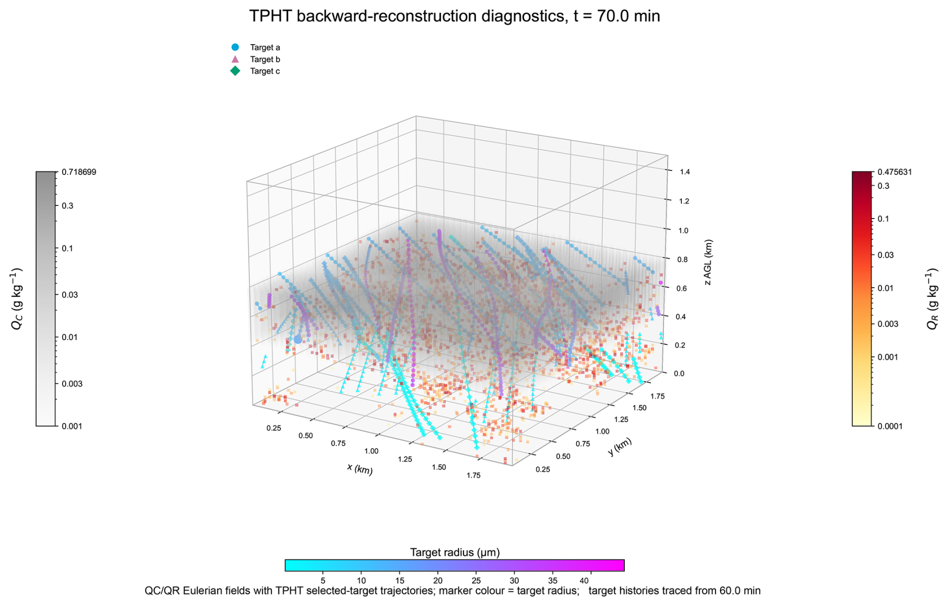
Figure 6 TPHT diagnostic visualisation for three selected targets at 70 min in the three-dimensional demonstration case. Grey shading shows the Eulerian cloud water mixing ratio (Q_C (g kg⁻¹)) field, plotted from smoothed grid-cell-centre markers for visualisation, and orange-red square markers show the rain water mixing ratio (Q_R (g kg⁻¹)) field without smoothing. The three TPHT-selected target histories are overlaid for the final 10 min, using circle, triangle, and diamond markers for the three targets; Target a, Target b, and Target c in the legend correspond to panels (a), (b), and (c) in Fig. 5, respectively. Marker and line colour indicate target radius. Trajectory line segments are not connected across periodic-boundary jumps. The visualisation places selected target histories in the contemporaneous cloud and rain fields and illustrates the diagnostic capability of interest-restricted backward reconstruction.

The three examples illustrate distinct diagnostic patterns. In Fig. 5a, the target first crosses the 15 µm threshold at about 30 min and around 600 m, associated with a target-linked coalescence record. It subsequently carries many additional coalescence-record links, especially after 60 min while descending, and reaches a radius exceeding 40 µm. In this example, the particle then evaporates near the cloud-base region rather than reaching the surface, and its reconstructed height indicates subsequent upward transport as a much smaller particle. In Fig. 5b, the target does not carry coalescence-record links during the first hour, and its reconstructed radius evolution before threshold crossing is consistent with condensational growth near cloud top during the final 10 min. The subsequent trajectory includes multiple linked coalescence records and a rapid increase in radius during descent. In Fig. 5c, the target does not reach the 15 µm threshold in the reconstructed output, but it carries several coalescence-record links. Its radius remains nearly unchanged, consistent with event records in which the target mainly changes multiplicity or participates as the smaller partner rather than growing substantially in radius.

These examples are intended to demonstrate TPHT diagnostic capability at the individual-target level. They show that the method can recover target-specific height–radius histories, first threshold-crossing positions, final-window target status, and associated coalescence-record timing.

The TPHT reconstruction also provides a compact way to inspect selected target histories in relation to the surrounding Eulerian cloud and rain fields. As an illustrative example, Fig. 6 overlays the three reconstructed target trajectories from the final 10 min of the 70 min TPHT demonstration on the Eulerian cloud-water and rain-water fields at 70 min. The trajectories are reconstructed from the backward selected-output records. Line segments are interrupted when a target crosses the periodic lateral boundary, so that the plotted path does not draw artificial connections across the domain. The visualisation shows that the selected targets can be followed through the cloud layer together with contemporaneous cloud water mixing ratio (Q_C) and rain water mixing ratio (Q_R) structures. Together with the predecessor-chain diagnostics in Fig. 5, this illustrates how TPHT connects individual target histories to the surrounding three-dimensional model fields.

Together, Figs. 5 and 6 show how the selected-population statistics in Sect. 3.4 can be linked to individual reconstructed histories and their surrounding cloud fields.

4 Discussion

4.1 Practical Implications of Tracking Workflows

The experiments highlight several practical differences among the tracking workflows: when the target set is defined, which identifiers and event records must be written, how much temporary and retained diagnostic output is produced, and how the resulting histories are reconstructed during post-processing. Forward tracking is appropriate when the target population can be specified before or during the model integration. Backward tracking is appropriate when the targets are known at the analysis stage, but its full-population configuration can become storage-limited because predecessor-link information must be written before the final target class is known. TPHT provides an intermediate strategy: a forward-discovery pass identifies an interest-defined target set, and a backward-reconstruction pass follows only the deduplicated targets.

The TPHT experiment illustrates both the value and the cost of this compromise. The forward-discovery pass generated many repeated interest-ID records because the same super-droplet can satisfy an interest condition at multiple times. Offline deduplication reduced these records to a compact target-list, and the backward-reconstruction pass recovered the deduplicated targets consistently. This demonstrates that the target-list can be used to connect event- or threshold-based discovery to backward reconstruction in a three-dimensional SDM simulation.

The storage interpretation is more nuanced than a single reduction factor. If raw discovery streams are retained, TPHT requires temporary working storage for the raw IDs, the deduplicated target list, and the reconstructed target output. If raw discovery streams are deleted after deduplication, the retained storage is dominated by the backward selected output and the compact target-list files. Therefore, TPHT should be interpreted as a workflow that separates temporary discovery output from retained diagnostic output. Its benefit depends on how sparse the interest criteria are, how frequently selected super-droplet states are written, and whether intermediate raw-ID streams are retained after the target list has been generated.

4.2 Limitations and Future Work

The same design choices that enable selected-target diagnostics also impose limitations on storage, target definition, sampling interpretation, and event-log analysis. The first limitation is storage and I/O cost. The direct lookup used in backward reconstruction reduces the search cost for a known predecessor-link pair, but it does not eliminate the need to write the predecessor-link information that will later be queried. The direct-lookup advantage can be interpreted as a record-level complexity reduction rather than as a measured wall-clock speed-up. If each predecessor query were performed by scanning all valid super-droplet records at the previous output time, the search cost would scale as O(N_tMN), where N_t is the number of saved output times, M is the number of reconstructed targets, and N is the number of valid records that would have to be searched at each output level. Using the saved predecessor-link pair reduces the lookup part to O(N_tM), because each predecessor query is a direct lookup once the rank and record index are known. A more efficient global-search baseline would scan all records once per output time, with cost O(N_tN). Relative to a global-pass baseline, the reduction in record-access operations can be written as $R_{\text{lookup}}=N/M$, where M is the number of reconstructed targets and N is the number of valid records at each saved output level. This factor increases as the queried target subset becomes sparser. It is a record-level complexity estimate rather than a measured wall-clock speed-up. More generally, if a fraction f of the valid super-droplet population is retained and per-record output dominates the file volume, the retained-output reduction approaches $\mathrm{1}/f$, subject to fixed file overhead and temporary discovery storage. TPHT can therefore provide orders-of-magnitude larger reductions for sufficiently sparse target classes. This estimate does not include NetCDF chunking, file caching, or other I/O effects, so it should be interpreted as a complexity estimate rather than a measured post-processing speed-up.

A full-population backward tracking configuration therefore remains expensive for large three-dimensional simulations with many output times and many variables. TPHT reduces this burden only when the interest-defined target set is sufficiently smaller than the full valid super-droplet population, and the practical retained-storage benefit also depends on whether temporary raw-ID streams are removed after deduplication.

A second limitation is that TPHT requires interest criteria to be specified before or during the discovery pass. In this study, radius-threshold exceedance and the binary coalescence flag were used as diagnostic criteria. Other questions would require different event definitions, for example entrainment, mixing, supersaturation exposure, sedimentation, or residence in a specified cloud region. TPHT does not provide arbitrary access to every super-droplet history after the fact; histories can only be reconstructed for targets that were captured by the discovery criteria or otherwise retained by the selected-output configuration.

The sampling tests also have a limited scope. The short quasi-two-dimensional sampling verification in Appendix B checks the sampling workflow and quantifies seed-to-seed variability for selected diagnostics, but it is not evidence of long-time or three-dimensional representativeness. In general, the representativeness of a selected target set depends on the sampling fraction, the stratification variables, the cloud regime, the output interval, and the diagnostic quantity. For this reason, sampled forward or backward tracking should be interpreted as selected-target diagnostics unless representativeness has been evaluated for the specific analysis.

Coalescence-event diagnostics also require careful interpretation. The if_coal variable is a binary interval marker indicating that at least one recorded coalescence event involved the selected target during the relevant output interval. It is not an event counter. Similarly, target-linked coalescence records identify logged event links that can be inspected together with the reconstructed target history, but they should not be treated as a complete causal process budget unless all required event branches, multiplicities, and output variables have been retained and analysed for that purpose.

The present TPHT implementation uses raw interest-ID streams and offline deduplication. This design avoids maintaining a large in-memory set of previously detected IDs during the SDM integration, but it creates temporary working files that can be large when the interest criteria are broad. Future workflow optimisation could include parallel streaming deduplication, optional compression of raw ID streams, automatic deletion of raw streams after a verified target list, and richer logging of merge/deduplication wall-clock time. Such diagnostics would make the separation between model-integration cost, temporary working storage, and retained analysis storage more explicit.

For the two TPHT integrations to follow the same stochastic realisation, they must use the same source and executable, compiler and floating-point settings, numerical libraries, initial physical and random-number states, MPI rank count and decomposition, effective thread count, floating-point operation ordering, and physical random-number call order. A common practical check of simulation-level reproducibility would be to compare Eulerian output from the two integrations. In this demonstration, however, the forward-discovery run did not save Eulerian history or selected-super-droplet state output because these outputs were disabled to reduce storage. A comparison of the final Eulerian output therefore could not be performed from the archived filesInstead, the complete coalescence-event logs were compared as a code-level verification of TPHT. All examined physical event fields agreed bitwise, confirming that the recorded coalescence history was reproduced under the tested configuration. This result does not establish equality of every later Eulerian or super-droplet state, nor does it imply bitwise reproducibility across arbitrary compilers, hardware, MPI decompositions, effective thread counts, code versions, or changes in floating-point operation ordering or random-number call ordering.

A natural future extension is to generalise TPHT interest criteria beyond radius and coalescence flags. Event- and history-based Lagrangian diagnostics have been used to study entrainment, mixing, and cloud-life-cycle states (Lim and Hoffmann, 2023, 2024). Similar criteria could be implemented in SCALE-SDM using entrainment indicators, supersaturation histories, activation or deactivation events, sedimentation, local turbulence measures, or residence in cloud-top and cloud-base regions. The same target-list mechanism could then be used to reconstruct histories for particles satisfying these more specialised diagnostic conditions. Although the implementation described here is specific to SCALE-SDM super-droplets, the underlying design is not intrinsically limited to the Super-Droplet Method. The same ideas require particle-like entities with persistent identifiers, well-defined ownership during parallel exchange, saved predecessor links, and event records. The interpretation of the tracked object remains model-specific: in SCALE-SDM, an identifier refers to a super-droplet with multiplicity rather than to an individual real droplet. Applying the framework to other Lagrangian particle models would therefore require model-specific definitions of particle identity, event participation, and output variables.

The present implementation focuses on warm-cloud microphysics. Extending the tracking workflows to ice-phase processes is a valuable direction for future work, for example to diagnose the histories of riming and aggregation events or to identify the origins of secondary ice particles. The identifier, event-log, and target-list concepts described here provide a technical basis for such an extension, although the ice-phase implementation would require additional process-specific event definitions and output variables. More broadly, selected-target histories and event-log diagnostics from particle-based models can provide process-level constraints for evaluating microphysical parameterisation schemes used in larger-scale weather and climate models. Such applications would require dedicated comparisons with the variables and assumptions used in those parameterisations.

5 Summary and Conclusions

This study documents and evaluates a Lagrangian particle-tracking framework implemented in SCALE-SDM. The framework includes forward tracking, backward tracking, and two-pass hybrid tracking (TPHT). Forward tracking assigns persistent identifiers to selected target super-droplets and writes their subsequent selected-output records. Backward tracking writes for each selected record, the location of its predecessor at the previous output time, allowing direct retrieval during post-processing. TPHT combines these two model integrations: the first identifies particles that meet prescribed radius or coalescence conditions, and the second reconstructs only those particles from the same initial state.

The implementation is designed to distinguish full-population backward tracking from target-restricted reconstruction. Full-population backward tracking preserves broader a posteriori flexibility, but its storage and I/O cost can become limiting in three-dimensional simulations because predecessor-link information must be written before the final target class is known. TPHT addresses this limitation for predefined diagnostic questions by replacing arbitrary full-population reconstruction with interest-restricted target discovery and reconstruction. In the present demonstration, the interest criteria were radius-threshold exceedance and participation in recorded coalescence events.

Controlled computational tests were used to quantify the tracking overhead. In the sampled three-dimensional benchmark, the 5 % sampled forward and backward tracking configurations did not show a large wall-clock or peak RAM penalty relative to the no-tracking baseline. The main additional burden was selected-super-droplet output and coalescence-event diagnostics. SDNC-scaling and output-interval tests further showed that output burden depends on the number of selected records and output frequency. A short quasi-two-dimensional sampling test was used to verify the sampling workflow and to quantify seed-to-seed variability, but it was not interpreted as evidence for long-time three-dimensional representativeness.

The TPHT demonstration was performed in a three-dimensional DYCOMS-II RF02 stratocumulus configuration. The forward-discovery pass generated 27 826 660 866 identifier records because an identifier was written each time a particle met a selection condition. The target-list transfer recovered all 3 554 256 unique target identities without missing or additional identities. To verify the TPHT implementation beyond this ID-transfer check, the complete coalescence-event logs from the two runs were compared. All 2 919 183 records agreed bitwise in event time, particle radii, multiplicities, and represented collision count, confirming that the recorded coalescence history was reproduced under the tested configuration.

The TPHT storage results show the importance of distinguishing temporary working storage from retained analysis storage. The raw interest-ID streams occupied 245 GiB, but they are temporary files that can be deleted after deduplication. The deduplicated per-rank target-list files occupied only 32.0 MiB, and the backward selected-super-droplet output occupied 69 GiB. If the raw discovery streams are retained, the total TPHT working storage was 314 GiB, corresponding to an estimated 1.1× reduction relative to the estimated full-population backward output of 356 GiB. After raw-ID deletion, the retained output was dominated by the backward selected output and compact target-list files, corresponding to an estimated retained-output reduction of about 5.2×. This storage benefit depends on the sparsity of the interest criteria, the output interval, the variables written, and whether raw discovery streams are retained after target-list generation.

The stratocumulus case study was used as a methodological demonstration rather than as a new cloud-physics interpretation. The comparison between the Hall gravitational collection kernel and TPHT-linked coalescence records provides radius-pair context for the coalescence-participation criterion. The TPHT target diagnostics characterise the reconstructed target set, including radius-threshold and coalescence-flag categories, first threshold-crossing heights, and near-threshold radius behaviour. The predecessor-chain examples and three-dimensional trajectory visualisation further demonstrate how TPHT can connect population-level target selection to individual reconstructed histories and contemporaneous Eulerian cloud and rain fields.

Several limitations remain. TPHT requires the interest criteria to be specified before or during the discovery pass and does not provide unrestricted access to every super-droplet history after the fact. The if_coal variable is a binary interval marker rather than an event counter, and target-linked coalescence records should be interpreted as diagnostic event-log links rather than a complete process budget. The present sampling verification is limited to a short quasi-two-dimensional setup. Future work should therefore extend the workflow to additional event definitions, improve logging of offline merge and deduplication costs, explore compression or automatic cleanup of temporary raw-ID streams, and apply the same identifier and event-log concepts to ice-phase processes such as riming, aggregation, and secondary ice production. More broadly, selected-target histories from particle-based models can provide useful constraints for evaluating microphysical parameterisation schemes, provided that the diagnostic variables are matched carefully to the assumptions and scales of those schemes.

Appendix A: Controlled Computational Benchmark

Figure A1 summarises the controlled cold-start three-dimensional benchmark used to quantify the computational cost of sampled tracking diagnostics. All cases used the DYCOMS-II RF02 configuration in a full three-dimensional domain of 2 km × 2 km × 1.5 km, with grid spacing of 50 m × 50 m × 5 m, corresponding to a 40 × 40 × 300 grid. The integration time was 1800 s, and the super-droplet number concentration was 40 per cell. The benchmark was run from a cold start and was intended as a computational-overhead test of the tracking diagnostics, not as a mature-cloud physical validation experiment.

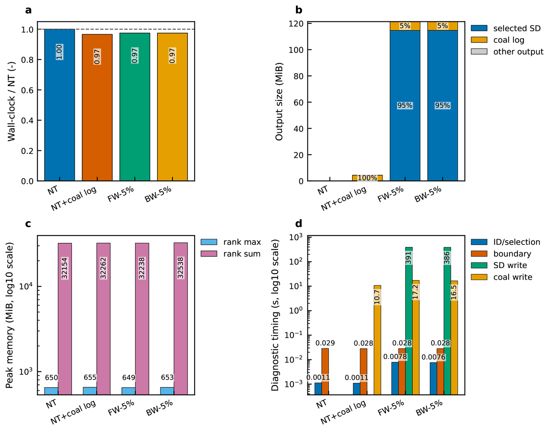
Figure A1 Controlled cold-start benchmark overhead for sampled tracking diagnostics. (a) Wall-clock time normalised by the no-tracking/no-coalescence-log case (NT). (b) Scientific output volume, separated into selected-super-droplet output (SD_selected_NetCDF_^∗), coalescence-event log output (SD_coal_output_NetCDF_^∗), and other output. (c) Peak-memory diagnostics, where “Peak memory” denotes the peak resident RAM measured from the rank-level resident-memory high-water mark. The bars show the maximum single-rank value and the sum of the rank-level peak values across MPI ranks. (d) Instrumented diagnostic timings for identifier assignment or selection bookkeeping, boundary-tracking exchange, selected-super-droplet output writing, and coalescence-event log writing. The timing diagnostics are subcomponent measurements and are not additive estimates of total model runtime.

The case NT disables both tracking and coalescence-event logging, whereas NT + coal log enables only coalescence-event output to SD_coal_output_NetCDF_^∗. The sampled forward- and backward-tracking cases use 5 % stratified target selection, write selected-super-droplet output to SD_selected_NetCDF_^∗ every 60 s, and also enable coalescence-event logging.

The plotted variables separate wall-clock cost, output volume, RAM use, and instrumented diagnostic timings. The relative wall-clock time is the elapsed runtime normalised by the no-tracking/no-log baseline. Scientific output is decomposed into selected-super-droplet output, coalescence-event log output, and other scientific output. Peak RAM is reported both as the maximum single-rank peak RAM and as the sum of peak RAM over MPI ranks, based on rank-level resident-memory diagnostics. The timing panel includes identifier assignment or selection bookkeeping, boundary-tracking exchange, selected-super-droplet output writing, and coalescence-event output writing. These timing diagnostics are subcomponent measurements and should not be summed to reconstruct the total wall-clock time.

In this benchmark, the sampled forward- and backward-tracking cases remain close to the no-tracking baseline in normalised wall-clock time. Values slightly below the NT case should not be interpreted as a speed-up. Because only one run was available per configuration, the small wall-clock differences cannot be separated from unquantified scheduler and file-system variability; the results show only that no large wall-clock penalty was detected. The main additional burden appears in output volume. The sampled tracking cases produce about 121 MiB of scientific output, of which approximately 95 % is selected-super-droplet output and about 5 % is coalescence-event log output. Peak RAM changes only weakly across the four cases. Among the instrumented timings, selected-super-droplet output writing is the dominant additional component, whereas identifier bookkeeping and boundary-tracking exchange are much smaller. Thus, for this sampled configuration, the practical overhead is dominated by diagnostic output rather than by tracking-identifier bookkeeping.

Table A1 Normalised metrics for the 30 min controlled three-dimensional benchmark. Wall-clock time is normalised by simulated duration and by the 18 000 model steps. Core-hours use 64 MPI ranks and one effective thread per rank. Selected-output bytes per written record use the sum of super-droplet numbers over all selected-output files; repeated records from the same target at different output times are counted separately. Coalescence-log bytes per event include NetCDF and sparse rank-file overhead. Peak RAM is the maximum rank-level resident-memory high-water mark. Only one run was available per configuration, so small wall-clock differences are not interpreted as statistically resolved speed-ups or overheads. n/a denotes not applicable.

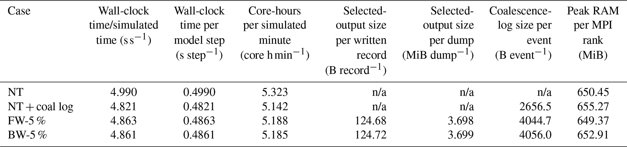
Normalising the 30 min benchmark gives 4.82–4.99 wall-clock seconds per simulated second, equivalent to 0.482–0.499 s per 0.1 s model step, and 5.14–5.32 core-hours per simulated minute (Table A1). Forward and backward selected output required 124.68 and 124.72 bytes per written target record, respectively, or about 3.70 MiB per scheduled output time. Peak RAM was 649–655 MiB per MPI rank. Because only one run was available for each configuration and the no-tracking run was the slowest, the benchmark does not resolve a statistically supported speed-up or a small tracking overhead; it shows only that no large penalty was detected under this configuration.

Appendix B: Sampling-procedure Verification

The common target-selection and sampling procedure described in Sect. 2.4 is evaluated using a short quasi-two-dimensional verification case. The purpose of this test is to check the implementation of the random and stratified sampling workflows and to quantify seed-to-seed variability in a controlled setup. The test is not intended to establish long-time or three-dimensional representativeness.

The common configuration used a quasi-two-dimensional domain of 6 km × 0.1 km × 1.5 km with grid spacing of 50 m × 50 m × 5 m. The integration time was 600 s, the super-droplet number concentration was 40 per cell, and forward tracking was enabled with the namelist parameter “tracking_mode = 1”. Selected-super-droplet output was written every 60 s, Eulerian history output was disabled, and coalescence-event output was enabled.

Two full-reference runs were used: “random_full” for the random-sampling design and “stratified_full” for the stratified-sampling design. Random sampled runs were performed with sampling fractions of 0.05, 0.10, and 0.20, using 10 independent sampling seeds for each fraction. Stratified sampled runs used the same sampling fractions and the same number of seeds. For stratified sampling, candidate super-droplets were restricted to heights between 400 and 800 m and radii r≥ 1 µm, and were then grouped into 8 height bins and 10 logarithmic radius bins. Random sampled cases are compared against random_full, and stratified sampled cases are compared against stratified_full. This avoids mixing two different candidate definitions and means that absolute errors should be interpreted within each sampling design rather than as a direct ranking between random and stratified sampling.

The main error metric is the droplet-size-distribution (DSD) L1 error, which is computed from multiplicity-weighted, normalised radius histograms. For each selected-output time t, the sampled case contains super-droplets with radii r_i(t) and multiplicities n_i(t), where n_i corresponds to the super-droplet multiplicity variable sd_n. The corresponding full-reference case contains radii $r_j^{\text{ref}}\left(t\right)$ and multiplicities $n_j^{\text{ref}}\left(t\right)$. For each sampled-reference comparison and output time, the upper radius bound is defined as

$$\begin{array}{}\text{(B1)}& R_{\text{max}}\left(t\right)=\text{max}\left(\underset{i}{\text{max}}{r}_i\left(t\right),\underset{j}{\text{max}}{r}_j^{\text{ref}}\left(t\right),\mathrm{25}\mathrm{\mu }\mathrm{m}\right).\end{array}$$

We first define 31 bin edges, which form 30 linearly spaced radius bins:

$$\begin{array}{}\text{(B2)}& e_k\left(t\right)={\displaystyle \frac{k{R}_{\text{max}}\left(t\right)}{\mathrm{30}}},k=\mathrm{0},\mathrm{\dots },\mathrm{30}.\end{array}$$

The 30 histogram bins are then indexed by $k=\mathrm{1},\mathrm{\dots },\mathrm{30}$, with bin k corresponding to the interval $\left[e_{k-\mathrm{1}}\right(t),e_k(t\left)\right)$. The final bin includes the right endpoint e₃₀(t). For bin $k=\mathrm{1},\mathrm{\dots },\mathrm{30}$, the multiplicity-weighted normalised sampled histogram is

$$\begin{array}{}\text{(B3)}& \begin{array}{rl}& P_k\left(t\right)={\displaystyle \frac{{\sum }_i{n}_i\left(t\right)\mathrm{1}\left[e_{k-\mathrm{1}}\right(t)\le r_i(t)<e_k(t\left)\right]}{{\sum }_i{n}_i\left(t\right)}},\\ & k=\mathrm{1},\mathrm{\dots },\mathrm{30}.\end{array}\end{array}$$

For k=30, the indicator includes the right endpoint r_i(t)=e₃₀(t). The corresponding full-reference histogram is

$$\begin{array}{}\text{(B4)}& \begin{array}{rl}& Q_k\left(t\right)={\displaystyle \frac{{\sum }_j{n}_j^{\text{ref}}\left(t\right)\mathrm{1}\left(e_{k-\mathrm{1}}\left(t\right)\le r_j^{\text{ref}}\left(t\right)<e_k\left(t\right)\right)}{{\sum }_j{n}_j^{\text{ref}}\left(t\right)}},\\ & k=\mathrm{1},\mathrm{\dots },\mathrm{30}.\end{array}\end{array}$$

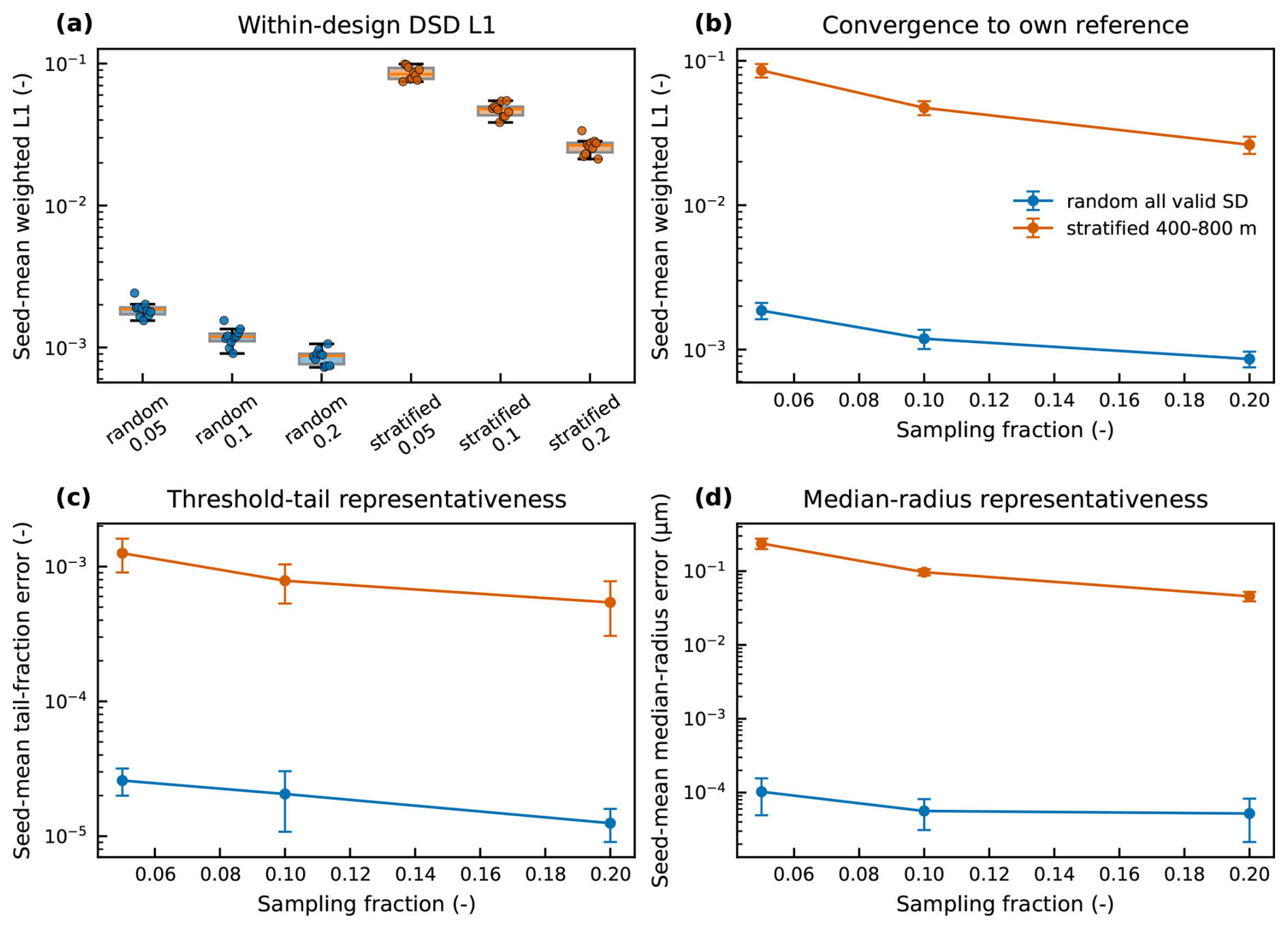
Figure B1 Short quasi-two-dimensional sampling-procedure verification. For each sampling design, sampled outputs are compared against the corresponding full-reference output: random samples are compared with random_full, and stratified samples are compared with stratified_full. The droplet-size-distribution (DSD) error is computed from normalised multiplicity-weighted radius histograms. Points and error bars in panels (b)–(d) show the mean and seed-to-seed standard deviation across 10 seeds after first averaging over output times for each seed. This test verifies the sampling workflow in a short two-dimensional setup and is not used as evidence for long-time three-dimensional representativeness.

For k=30, the final bin includes the right endpoint for both P_k(t) and Q_k(t). The DSD L1 error at time t is then defined as

$$\begin{array}{}\text{(B5)}& \mathrm{L}{\mathrm{1}}_{\text{DSD}}\left(t\right)={\sum }_{k=\mathrm{1}}^{\mathrm{30}}\mathrm{|}{P}_k\left(t\right)-Q_k\left(t\right)\mathrm{|}.\end{array}$$

No factor of $\mathrm{1}/\mathrm{2}$ is applied, so this is the histogram L1 distance rather than the total variation distance. Because both histograms are normalised, L1_DSD is dimensionless and ranges from 0 to 2, where 0 indicates identical sampled and full-reference histograms on the chosen radius bins.

For each seed, the time-mean error is computed as

$$\begin{array}{}\text{(B6)}& \mathrm{L}{\mathrm{1}}_{\text{DSD},\text{seed}}={\displaystyle \frac{\mathrm{1}}{N_t}}{\sum }_{t=\mathrm{1}}^{N_t}\mathrm{L}{\mathrm{1}}_{\text{DSD}}\left(t\right),\end{array}$$

where N_t is the number of selected-output times used in the verification. The values shown in Fig. B1 summarise L1_DSD,seed across the 10 independent sampling seeds for each sampling fraction and sampling mode.

This metric measures the total absolute difference between the sampled and reference normalised radius distributions. Because the histograms are normalised, the metric reflects the shape error of the multiplicity-weighted DSD rather than the total number of selected records.

Figure B1 summarises the sampling-procedure verification. The figure compares random and stratified sampling at sampling fractions of 5 %, 10 %, and 20 % against their corresponding full-reference outputs. Figure B1a shows the seed-level multiplicity-weighted DSD L1 error, Fig. B1b shows the decrease of the mean DSD L1 error with sampling fraction, Fig. B1c shows the error in the multiplicity-weighted fraction of droplets with radius greater than or equal to 15 µm, and Fig. B1d shows the error in the weighted median radius. For each seed, the diagnostics are first averaged over output times. Points and error bars then show the mean and seed-to-seed standard deviation across the 10 seeds for each sampling fraction and sampling design.

Within each sampling design, the multiplicity-weighted radius-distribution error generally decreases as the sampling fraction increases, indicating convergence toward the corresponding full-reference output in this short quasi-two-dimensional test. The spread across seeds quantifies sampling variability. These results support the implementation of the sampling procedure and show that increasing the retained fraction reduces sampling error for the tested diagnostics. However, the test should be interpreted as a procedure-level verification rather than as a general proof of three-dimensional representativeness for all cloud diagnostics.

In the 600 s quasi-two-dimensional verification, the number of written selected records increased approximately in proportion to the retained fraction over 5 %–20 % within both random and stratified selection modes. The ensemble was designed to evaluate sampling fidelity rather than fraction-only performance scaling. Changes in wall-clock time and peak RAM could not be resolved from the model-dominated runtime and seed-to-seed variability. Random and stratified results are evaluated against separate full references because their effective candidate populations differ.

Appendix C: Scalability and Output-Interval Sensitivity

Additional computational diagnostics were performed to support the computational and storage summary in Sect. 3.2.3. These tests characterised the sensitivity of the tracking workflow to the super-droplet number concentration (SDNC) and to the selected-super-droplet output interval. They are controlled diagnostic experiments and are not intended as mature-cloud physical analyses.

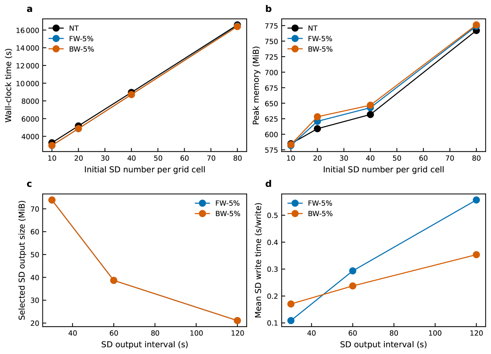
Figure C1 Scalability and selected-output-interval sensitivity diagnostics for the tracking experiments. The SDNC-scaling panels characterise the dependence of wall-clock time and peak RAM per rank on the super-droplet number concentration for the no-tracking baseline and sampled tracking configurations. The output-interval panels characterise the dependence of selected-super-droplet output size and mean write time per output operation on the selected-output interval. These controlled tests support the computational summary in Sect. 3.2.3 and should not be interpreted as asymptotic performance laws.

The common configuration used a full three-dimensional domain of 2 km × 2 km × 1.5 km with grid spacing of 50 m × 50 m × 5 m. Eulerian history output and coalescence-event output were disabled. Forward and backward tracking cases used stratified sampling with a sampling fraction of 0.05. Candidate super-droplets were restricted to heights between 400 and 800 m and radii r≥ 1 µm. The no-tracking cases provide compute baselines, while the sampled tracking cases quantify the additional diagnostic cost of selected-super-droplet output.

The SDNC-scaling experiment used SDNC values of 10, 20, 40, and 80 per cell. The corresponding experiment labels were sdnc10, sdnc20, sdnc40, and sdnc80, combined with no-tracking, forward tracking, and backward tracking configurations. The duration was 1800 s, and selected-super-droplet output was written every 60 s for the tracking cases. These experiments were used in Fig. C1 to characterise the response of wall-clock time and peak RAM to increasing SDNC.

The output-interval sensitivity experiment used SDNC = 40 per cell and a duration of 600 s. The no-tracking baseline was nt_nolog_10min. The forward and backward tracking cases used selected-super-droplet output intervals of 30, 60, and 120 s, corresponding to the experiment labels out30, out60, and out120. These experiments are used in Fig. C1 to characterise selected-output size and mean write-time behaviour as the output interval is varied.

Over the tested SDNC range, wall-clock time increases with SDNC, while the number of tracked chains scales approximately linearly with the number of super-droplets for a fixed sampling fraction. Peak RAM per rank increases only weakly over the same range. These results describe finite-range empirical behaviour for the tested machine configuration and should not be interpreted as general asymptotic scaling laws. The output-interval tests show the expected decrease in selected-output volume as the output interval increases. However, each output operation contains more records when the interval is longer, so the mean write time per output operation can increase even while the total number of output files decreases. Because SDNC was varied at a fixed 5 % tracking fraction, this experiment combines physical-model scaling with tracking-load and selected-output scaling. It therefore measures end-to-end behaviour as the physical super-droplet population and the tracked population increase together, but does not isolate the marginal overhead of changing the tracking fraction alone.