TRAILS – a novel framework for time-height-resolved attribution of long-range transported wildfire smoke

Accurately attributing long-range transported wildfire smoke to specific sources remains challenging, especially for elevated plumes. This study presents the TRAILS tool (Trajectory-based Identification of Lofted Smoke), which extends the automated air mass source attribution tool of Radenz et al. (2021) to provide time- and height-resolved identification of wildfire smoke. By integrating 10 d backward trajectories from FLEXPART with a multi-sensor satellite detection algorithm, we calculate a vertically resolved Smoke Occurrence Fraction (SOF), quantifying the likelihood of smoke influence based on air parcel residence time within smoke-affected regions. TRAILS identifies where and at what altitudes smoke is present, but does not automatically attributes these layers to specific fire sources. A key innovation is a new, statistically significant linear relationship between Ozone Mapping and Profiler Suite (OMPS) Ultraviolet Aerosol Index (UVAI) values and smoke plume height for fresh tropospheric smoke, derived from collocated OMPS and CALIOP observations. TRAILS was evaluated against ground-based measurements from the fluorescence lidar (MARTHA) and Raman lidar (Polly^XT) in Leipzig during the 2023 Canadian wildfire season. Results show that TRAILS effectively reproduces the vertical distribution and temporal evolution of long-range smoke layers, with a 76 % detection rate for fluorescent aerosol layers. Systematic underestimation of layer heights by 0.4 km, most pronounced in the UTLS, is consistent with unaccounted diabatic self-lofting in FLEXPART. While TRAILS performs well for the Northern Hemisphere smoke events studied here, its application to other wildfire regimes (e.g., Southern Hemisphere, different fuel types) may require recalibration of thresholds and carries additional uncertainties related to dust contamination. TRAILS provides a valuable, observationally constrained method for time-height-resolved smoke attribution, particularly where advanced fluorescence lidars are unavailable.

1 Introduction

Concurrent heatwaves and droughts have become more frequent, a trend that is projected to continue with global warming. These conditions have intensified fire weather, characterized by hot, dry, and windy events, which are becoming increasingly probable in some regions (Intergovernmental Panel On Climate Change (IPCC), 2023; Potapov et al., 2025). Fire weather increases the risk of the occurrence of wildfires as well as their intensity (Dowdy et al., 2019). In extreme cases, fire-triggered thunderstorms (pyrocumulonimbus, or short for pyroCb) can release large quantities of smoke particles into the upper troposphere and lower stratosphere, in amounts comparable to the mass released by a volcanic eruption (Peterson et al., 2021; Fromm et al., 2021). These particles may persist for months, circulating globally (Khaykin et al., 2020; Ohneiser et al., 2022).

Within the atmosphere smoke particles impact Earth's radiative balance both directly, by interacting with solar radiation (Hirsch and Koren, 2021; Das et al., 2021), and indirectly, by acting as cloud condensation nuclei (CCN) and ice-nucleating particles (INPs) that alter cloud formation (Knopf et al., 2018). Ground-based lidar observations over the Arctic and Europe confirm that aged, long-range transported smoke can trigger cirrus cloud development (Mamouri et al., 2023; Ansmann et al., 2023, 2025; Gast et al., 2025). As the optical properties of smoke aerosols can vary significantly, their identification and classification remains challenging (Floutsi et al., 2023). Laser-induced fluorescence observations improve the detection of biogenic particles within the atmosphere (Reichardt et al., 2025), particularly in detecting biomass burning aerosols (Hu et al., 2022; Gast et al., 2025). Yet, distinguishing wildfire smoke from other fluorescent particles such as pollen or urban aerosols remains a complex task when smoke is for example mixed into the lower troposphere or the planetary boundary layer (PBL) (Veselovskii et al., 2024; Miri et al., 2025). In such cases, information about the source of the fluorescent aerosol layer would be highly valuable.

Aerosol layer source attribution is usually achieved using backward trajectories combined with geographical data like the automated air mass source attribution tool developed by Radenz et al. (2021). This tool provides continuous, vertically resolved estimates of air mass origins above a given location. It combines backward airmass transport simulations from a dispersion model with geographical data, including land cover classifications and manually defined geographical regions. The tool can be used operationally and is already widely used in smoke-cloud interaction studies like Baars et al. (2021), Haarig et al. (2022), Ansmann et al. (2023). In general, the method assumes that an air parcel takes up the properties of the surface when its traveled path is close to the ground. Proximity to the surface is determined by the so-called reception height, typically defined as either the model-derived PBL height or a fixed threshold of 2 km (Val Martin et al., 2010). As noted by Radenz et al. (2021), the tool can also be particularly useful for studying events involving elevated aerosol emissions, such as wildfire smoke or volcanic eruptions. However, its fixed reception height is a major limitation, as smoke plume injection heights are highly variable and cannot be generalized to a single altitude (Val Martin et al., 2010).

The challenge of tracking smoke emissions by means of static emission heights is further complicated by a dynamic process known as smoke self-lofting. Smoke is highly absorptive in the shortwave spectrum. Optically thick smoke layers can heat the ambient air through absorption of solar radiation, generating buoyancy that causes the layer to ascend (Torres et al., 2020; Ohneiser et al., 2023). The self-lofting rate depends on several factors, most importantly including the aerosol optical thickness (AOT), the smoke injection height, and the aerosol chemical composition. For a comprehensive discussion, see Ohneiser et al. (2023). Model simulations for the troposphere indicate that a smoke layer initially at 4 km can be lifted to the tropopause within approximately 4.5 d, given a 500 nm AOT of 0.5 and a varying black carbon fraction of 5 % to 15 % to account for aging (Ohneiser et al., 2021). Using the Community Earth System Model (CESM), Huang et al. (2026) demonstrated that incorporating self-lofting for tropospheric smoke plumes improved the agreement between modeled and observed smoke plume heights from the 2019–2020 Australian New Year (ANY) wildfires. During the MOSAic (Multidisciplinary drifting Observatory for the Study of Arctic Climate) expedition, smoke from the 2019 Siberian wildfires was observed at an altitude of 12 km over the German icebreaker Polarstern. Due to the lack of pyroCb activity self-lofting has been suggested as the mechanism that transported the smoke from the lower troposphere up to the upper troposphere and lower stratosphere (UTLS) (Ohneiser et al., 2021). In contrast, self-lofting has been extensively studied in the stratified stratosphere, where more stable conditions favor the development of coherent, long-lived smoke layers. As noted by Ohneiser et al. (2023), tropospheric smoke layers are typically more vertically stretched, making them more susceptible to disruption by wind shear and turbulence in the less stratified troposphere. For instance, following the 2017 Canadian wildfires, CALIOP lidar observations recorded lofting rates of up to 1 km d⁻¹, associated with a 532 nm AOT of 0.7 and a black carbon ratio of 2.5 % (Ohneiser et al., 2023).

Satellite remote sensing enables the global tracking of the horizontal and vertical distribution of smoke plumes. This is achieved through sensors that measure aerosol radiation absorption, either quantitatively (e.g., single scattering albedo, SSA; aerosol absorption optical depth, AAOD) or qualitatively (e.g., UV Aerosol Index, UVAI) (Herman et al., 1997; Torres et al., 1998). Several operational UV-capable sensors currently retrieve near-UV aerosol properties. For instance, the Ozone Monitoring Instrument (OMI) aboard the low Earth orbit (LEO) Aura satellite (2004–present) offers a pixel size of 13 × 24 km and supports two aerosol algorithms: OMAERO (KNMI) and OMAERUV (NASA) (Torres et al., 2007, 2013). Since ∼ 2007, OMI observations have been degraded by the row anomaly, reducing effective coverage (Torres et al., 2018). The Ozone Mapping and Profiler Suite Nadir Mapper (OMPS-NM) on the Suomi-NPP satellite (launched 2011) provides observations at 50 km resolution, with data available from January 2012 to present (Kramarova et al., 2014). The Earth Polychromatic Imaging Camera (EPIC) aboard NOAA's DSCOVR spacecraft at the L1 point retrieves near-UV AOD and SSA (Ahn et al., 2021) as well as O₂-B–based aerosol layer height (ALH) at 18 × 18 km resolution since June 2015 (Xu et al., 2019; Torres et al., 2025). Since 2018, the Tropospheric Monitoring Instrument (TROPOMI) on ESA's Sentinel-5 Precursor satellite has provided global products of aerosol properties at a high spatial resolution of of 5.5 × 3.5 km (improved from 7 km × 3.5 km since August 2019), including UVAI, AOD, SSA, and ALH. EPIC and TROPOMI provide dedicated ALH products that rely on Oxygen-A and Oxygen-B band measurements. OMPS-NM, in contrast, does not provide a dedicated height product but offers the longest continuous UVAI record available, extending back to 2012 (Kramarova et al., 2014).

In the presented study, we build upon the study of Radenz et al. (2021) to attribute lidar-detected aerosol layers to wildfire smoke using output from the Lagrangian dispersion model FLEXPART (Pisso et al., 2019), and for the first time combine it with global smoke layer information derived from UVAI measurements from OMPS-NM. Additionally, we establish a relationship between UVAI and smoke plume heights using CALIPSO lidar observations, distinguishing between fresh tropospheric smoke and aged stratospheric smoke. Our empirically derived smoke height constraint from OMPS-NM UVAI is intentionally simpler compared to EPIC's and TROPOMI's ALH algorithms, which account in greater detail for surface and cloud contamination effects. However, OMPS-NM provides the longest continuous UVAI record currently available, extending back to 2012 (Kramarova et al., 2014) and unaffected by the row-anomaly-related degradation that has limited OMI since 2007 (Torres et al., 2018). As our processing chain spatially averages all products to a common 1° grid to constrain computational cost, OMPS-NM's coarser native resolution compared to the other sensors incurs no practical disadvantage while still reducing data volume and processing time. Taken together, our approach is computationally more efficient, requires less data storage, and is sufficient for the categorical smoke classification required in this study.

Additionally active fire data from Moderate Resolution Imaging Spectroradiometer (MODIS) sensor on board the Aqua and Terra platform or from the Visible Infrared Imaging Radiometer Suite (VIIRS) instruments aboard the Suomi National Polar-orbiting Partnership (Suomi-NPP) can be used for smoke identification close to fire sources. In this study we used the latest collection of MODIS active fire products (MCD14ML) (Giglio et al., 2016) and the VIIRS 375 m active fire product VNP14IMGML (Schroeder et al., 2014), both of which can be downloaded from the Fire Information for Resource Management System (FIRMS) website.

The results of time-height resolved smoke attribution product are then compared and validated against ground-based fluorescence lidar observations. This approach is particularly valuable for ground-based remote sensing studies of aerosol-cloud interactions when fluorescence-capable lidars are unavailable.

The structure of the paper is as follows. Section 2 provides an overview of the remote sensing instruments and data products used. Section 3 details the methodology for the air mass source and smoke attribution algorithm. Section 4 presents and discusses case studies evaluating the tool's performance during the 2023 Canadian wildfire season, using ground-based lidar observations from Leipzig, Germany. Section 5 provides a statistical validation of the smoke occurrence fraction (SOF) against independent fluorescence lidar measurements. Finally, Sect. 6 summarizes the conclusions and outlines potential for future work.

2 Remote Sensing of wildfire smoke

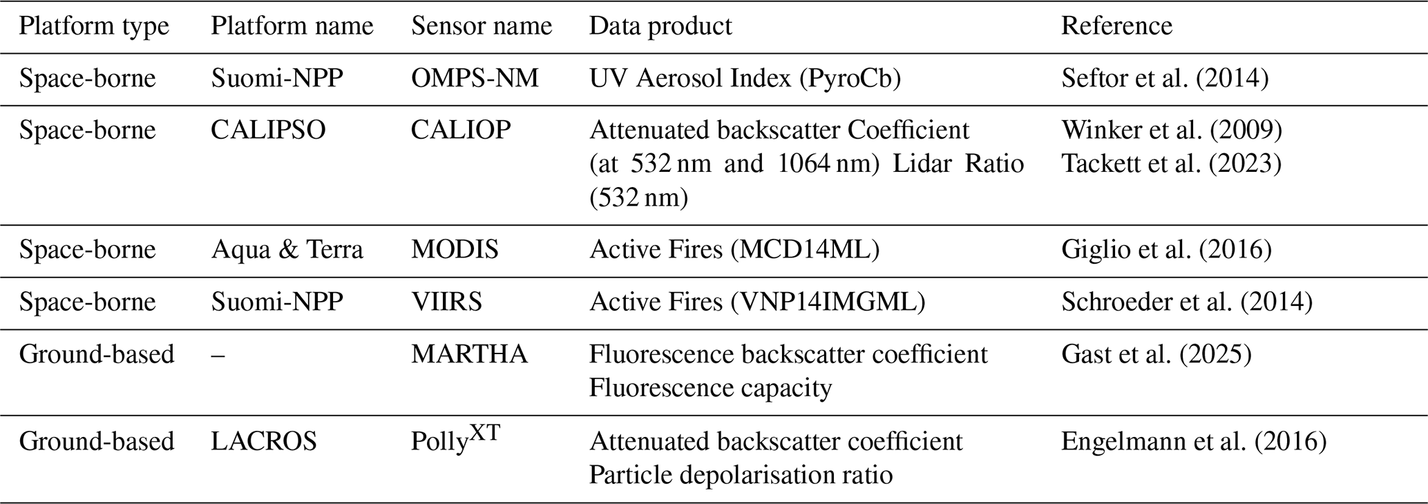
Satellite remote sensing enables global-scale observation of fires and smoke plumes, capturing their horizontal and vertical extent as well as long-range transport. In contrast, ground-based lidar remote sensing enables observations of aerosol profiles with very high temporal and vertical resolution. Table 1 provides a general overview of the different data products used in this study, which are introduced in more detail in the following sections.

Seftor et al. (2014)Winker et al. (2009)Tackett et al. (2023)Giglio et al. (2016)Schroeder et al. (2014)Gast et al. (2025)Engelmann et al. (2016)

Table 1 Overview of data products used within this study. MODIS = Moderate Resolution Imaging Spectroradiometer; VIIRS = Visible Infrared Imaging Radiometer Suite; Suomi-NPP = Suomi National Polar-orbiting Partnership, MARTHA = Multi-wavelength Atmospheric Raman lidar for Temperature, Humidity and Aerosol profiling, Polly^XT = PortabLe Lidar sYstem with eXTended capabilities.

2.1 CALIPSO

From June 2006 until August 2023, the Cloud-Aerosol Lidar with Orthogonal Polarization (CALIOP) aboard the Cloud-Aerosol Lidar and Infrared Pathfinder Satellite Observations (CALIPSO) satellite has provided the scientific community with continuous, vertically resolved data on the global distribution of atmospheric aerosols. The elastic-backscatter lidar features three measurement channels. Linearly polarized light pulses at 532 and 1064 nm are transmitted by the laser system. The detectors measure both cross- and co-polarized backscatter components at 532 nm and the total (cross + co-polarized) signal at 1064 nm. Here, “cross” and “co” refer to backscattered light polarized orthogonally and parallel, respectively, to the transmitted laser's polarization plane. A summary of the retrieval algorithms is provided by Winker et al. (2009). The basic measurement products include the attenuated backscatter coefficients at 532 and 1064 nm, and the volume linear depolarization ratio (defined as the ratio of the cross-polarized to co-polarized signal components). Figure 1 shows an overview of CALIOP observations from 18 July 2014. Enhanced backscatter coefficients reveal a smoke plume originating from British Columbia wildfires, along with cirrus clouds.

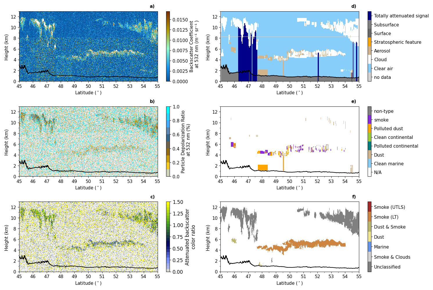
Figure 1 CALIOP observations from 18 July 2014 (20:33–20:36 UTC) reveal smoke from wildfires in British Columbia, Canada transported into the troposphere. The panels depict: (a) 532 nm attenuated backscatter coefficient, (b) particle depolarization ratio, and (c) attenuated backscatter color ratio. For comparison, (d) shows CALIPSO's Cloud-Aerosol Discrimination (CAD) output, while (e) displays the standard CALIPSO aerosol subtype classification. The smoke plume classification (distinguishing UTLS and lower troposphere (LT) layers) used in this study is shown in (f)). The black line denotes the surface elevation.

Within the Cloud and Aerosol Discrimination (CAD) algorithm of the CALIOP data processing sequence, clouds are distinguished from aerosols using multidimensional probability density functions derived from an extensive training set of CALIOP measurements (Liu et al., 2019). Subsequently, aerosol types are classified using predefined lidar ratios from the Lidar Level 2 Aerosol Profile (Version 4.51) product (Winker, 2026b) as detailed in Kim et al. (2018); Tackett et al. (2023). Although the CAD algorithm (Versions 3–4) improved smoke identification, we observe misclassification of smoke plumes as clouds, which is a known issue reported by Tackett et al. (2023). This arises from overlapping attenuated backscatter color ratios (0.5–0.9) and attenuated backscatter coefficients (0.004–0.01 m⁻¹ sr⁻¹) between dense smoke and clouds (Fig. 1c, d, e), preventing an unambiguous classification (Liu et al., 2009). The color ratio, which is the ratio of the backscatter coefficient at two wavelengths, serves as a proxy for particle size, with higher values typically indicating the presence of larger particles. For smoke, rapid signal attenuation at 532 nm (vs. 1064 nm) results in larger layer-averaged attenuated color ratios, further biasing classification toward clouds. This effect is evident in Fig. 1c, where below the smoke plume at approximately 5 km, the color ratio increases rapidly from 0.5 to above 1.5. Consequently, the known limitations of the standard CAD algorithm can lead to underestimation of smoke. To resolve this for our analysis, we implemented a custom classification scheme that allows the accurate identification of plume altitude for our case studies. These smoke plume altitude boundaries are then used to derive an altitude relationship with Suomi-NPP OMPS UVAI in Sect. 3.3.

To identify aerosol and cloud features, we utilize the attenuated backscatter coefficient at 532 nm (β₅₃₂) from the CALIOP Level 1B Profile data product (Version 4.51) (Winker, 2026a). Boundaries of aerosol plumes and clouds are enhanced using denoising and Gaussian filtering techniques to isolate coherent features. A percentile cutoff converts the smoothed backscatter into a binary mask, preserving only the strongest aerosol and cloud structures. This method maintains the original Level 1B resolution of 333 m. Object-based feature detection (Van Der Walt et al., 2014, scikit-image) identifies separated clusters, outputting a labeled array where each distinct plume is assigned a unique integer. Here, a “cluster” is defined as a contiguous region of pixels classified as smoke, identified via connected-component labeling. Each distinct cluster is assigned a unique integer label, while multiple clusters may belong to the same smoke layer if the layer is horizontally fragmented. To discriminate smoke plumes from clouds, marine aerosol, dust, and volcanic plumes, we use the extinction-to-backscatter ratio also known as lidar ratio at 532 nm (S₅₃₂) from the Lidar Level 2 Aerosol Profile (Version 4.51) data product (Winker, 2026b) and the particle depolarization ratio δ₅₃₂ that can be estimated from individual profiles of the cross-polarized (⟂β₅₃₂) and total backscatter coefficients as:

$$\begin{array}{}\text{(1)}& {\mathit{\delta }}_{\mathrm{532}}^{⟂/\parallel }={\displaystyle \frac{⟂{\mathit{\beta }}_{\mathrm{532}}}{\parallel {\mathit{\beta }}_{\mathrm{532}}-⟂{\mathit{\beta }}_{\mathrm{532}}}}\end{array}$$

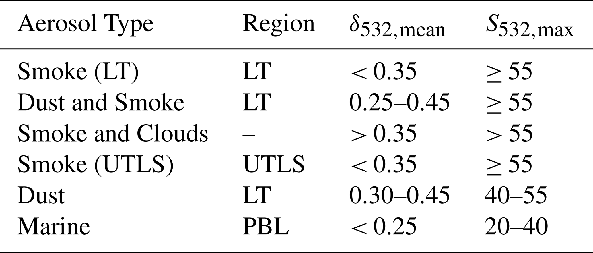
Each cluster is classified based on different thresholds for the cluster mean particle depolarization ratio δ_532,mean and the maximum lidar ratio S_532,max summarized in Table 2. The classification thresholds applied were derived empirically by testing a range of values for δ_532,mean and S_532,max across multiple CALIPSO overpasses and selecting the values that best reproduced the smoke boundaries identified through visual inspection. Smoke plumes are further separated into lower troposphere (LT) or upper troposphere-lower stratosphere (UTLS) regions using tropopause height data from the CALIOP L2 dataset. Note: This classification extracts boundaries for distinct smoke features, and does not intend to characterize complex aerosol mixtures (e.g. does not differentiate between smoke and polluted dust – see Fig. 1f).

Compared to the original CALIPSO atmospheric feature classification Fig. 1d), the smoke plume between 4–5 km is correctly identified by our classification method in panel (f). Moreover, our method shows similar mixed features (e.g., dust and smoke) compared to CALIPSO's aerosol classification (panel e). We classify features as smoke-cloud mixtures when parts of the feature meet the smoke lidar ratio threshold (S₅₃₂≥55 sr) and the feature-mean depolarization exceeds 35 %. This accounts for cirrus clouds' high depolarization (from non-spherical ice crystals).

Table 2 Aerosol and cloud classification criteria for different regions based on CALIPSO observations: lower troposphere (LT), upper troposphere and lower stratosphere (UTLS) and planetary boundary layer (PBL). Thresholds for the cluster mean particle depolarization ratio δ_532,mean and the maximum lidar ratio S_532,max are used to identify different aerosol types.

2.2 Suomi-NPP

The Ozone Mapping and Profiler Suite (OMPS) Nadir Mapper (NM), flown aboard the Suomi National Polar-orbiting Partnership (Suomi NPP) satellite, provides measurements of the ultraviolet Aerosol Index (UVAI). The concept of UVAI was introduced by Herman et al. (1997) and Torres et al. (1998) and has since become an invaluable tool for tracking the long-range transport of absorbing aerosols globally. Here we utilize UVAI generated by the NMMIEAI-L2 algorithm (version 2.1.1) (Torres, 2019). OMPS-NM has a nominal at-launch spatial resolution of about 50 km × 50 km.

The UVAI is a residual parameter that quantifies the difference in spectral dependence between measured and calculated outgoing radiances at the top of the atmosphere (TOA). For the calculation of radiances, Rayleigh scattering is assumed, and cloud scattering effects are parameterized. Global climatological data sets of Lambertian surface reflectivity are used to account for surface effects in the algorithm. Further information on the derivation of UVAI can be found in the README document in Torres (2019) and in Torres et al. (2018). For OMPS-NM, the UVAI is retrieved from the 340 and 378.5 nm wavelength channels (Torres, 2019). UV-absorbing aerosols, particularly smoke from biomass burning and desert dust, produce positive UVAI values. Non-absorbing aerosols in the UV produce negative UVAI values. A unique strength of the UVAI technique is that clouds produce nearly zero UVAI, and the presence of subpixel clouds does not significantly affect the detection of aerosols (Herman et al., 1997). Standard practice for filtering out cloudy pixels can be achieved using a UVAI threshold below 0.7 (Lee et al., 2015).

The UVAI of absorbing aerosols depends especially on the height of the aerosol layer and the aerosol optical depth (AOD). The AOD is influenced by the aerosol single scattering albedo, which depends on the imaginary refractive index and the particle size distribution (Herman et al., 1997; Torres et al., 1998). Aerosols that produce positive UVAI strongly absorb the molecular radiation coming from below the aerosol layer. Consequently, the higher the aerosol layer, the greater the amount of affected Rayleigh-scattered radiation that can be absorbed. This dependence is nearly linear and was established by Herman et al. (1997), Torres et al. (1998). The UVAI also increases linearly with AOD, with a slope proportional to the single-scattering albedo (Herman et al., 1997; Torres et al., 1998). For the 340 and 380 nm wavelength pair and a single layer of strongly absorbing aerosols, the linear increase with AOD continues until a value of approximately 2 (Stein Zweers, 2022). For AOD larger than 2, further increases in UVAI depend mainly on aerosol layer height (Ginoux and Torres, 2003; Torres et al., 2020). This effect diminishes with increasing single scattering albedo of the aerosol layer. Simulations of the UVAI sensitivities are described in Ginoux and Torres (2003), De Graaf et al. (2005). Model simulations show that the UVAI is further enhanced when the absorbing aerosol layer overlies a bright underlying scene. This occurs, for example, when liquid or ice clouds are located beneath or are embedded within the aerosol layer. The magnitude of the change in UVAI depends particularly on the cloud and aerosol optical depth and the aerosol single scattering albedo (Jethva and Torres, 2011; Torres et al., 2012). Moreover, the sensitivity of the UVAI to aerosol layer height is reduced when underlying clouds are present (Torres et al., 2012).

Guan et al. (2010) demonstrated that the UVAI, as measured by OMI, increases with plume height for fresh tropospheric and stratospheric smoke plumes exhibiting UVAI > 7. They pointed out that for young smoke plumes, which maintain sufficient optical thickness and stable single-scattering albedo (SSA), the primary driving factor of UVAI magnitude is plume height. They showed that UVAI is reduced in aged stratospheric plumes (4–5 d old), where dilution through mixing with clean air reduces aerosol optical depth and consequently UVAI. The authors further proposed that particle-aging processes play only a minor role in UVAI reduction, noting that the chemical and physical evolution of smoke occurs rapidly within the first hour after emission, with properties stabilizing thereafter for extended periods (hours to days) (Guan et al., 2010).

Peterson et al. (2021) report that UVAI values (for Suomi-NPP OMPS-NM) exceeding 15 typically indicate fresh stratospheric smoke plumes from extreme pyroCb events. For the Canadian wildfires in 2023, values exceeding 15 of the UVAI measured by OMPS-NM appeared in 5 cases between May and September, primarily between August–September when pyroCb activity was surprisingly low (Khaykin et al., 2020). Studies of such events, e.g., Khaykin et al. (2025), indicate that UVAI values larger than 10 are a strong indicator of pyroCb activity or smoke in the upper troposphere and lower stratosphere (UTLS).

Satellite-based wildfire and smoke detection is illustrated with an example case from the boreal summer of 2014. Strong wildfire activity was observed in the western part of North America (State of Washington and Northeast British Columbia) in July and August 2014. Active fires detected by MODIS (Aqua and Terra combined) between 16–18 July 2014 and the resulting wildfire smoke over Alberta and Montana on 18 July 2014 are evident from UVAI values exceeding 8 in Fig. 2. CALIOP backscatter coefficients (Fig. 3) indicate a smoke plume at approximately 5 km altitude during the overpass, marked by the blue dashed line in Fig. 2. We extract the respective grid points of the UVAI at the time of the CALIPSO overpass using the overpass time difference to Suomi-NPP combined with information about the 3D-wind field from ERA5 hourly data on the respective pressure levels of the smoke plume altitudes (Copernicus Climate Change Service, 2018). The extracted values of the UVAI can be seen in Fig. 3 together with the extracted smoke plume height from the CALIOP measurements.

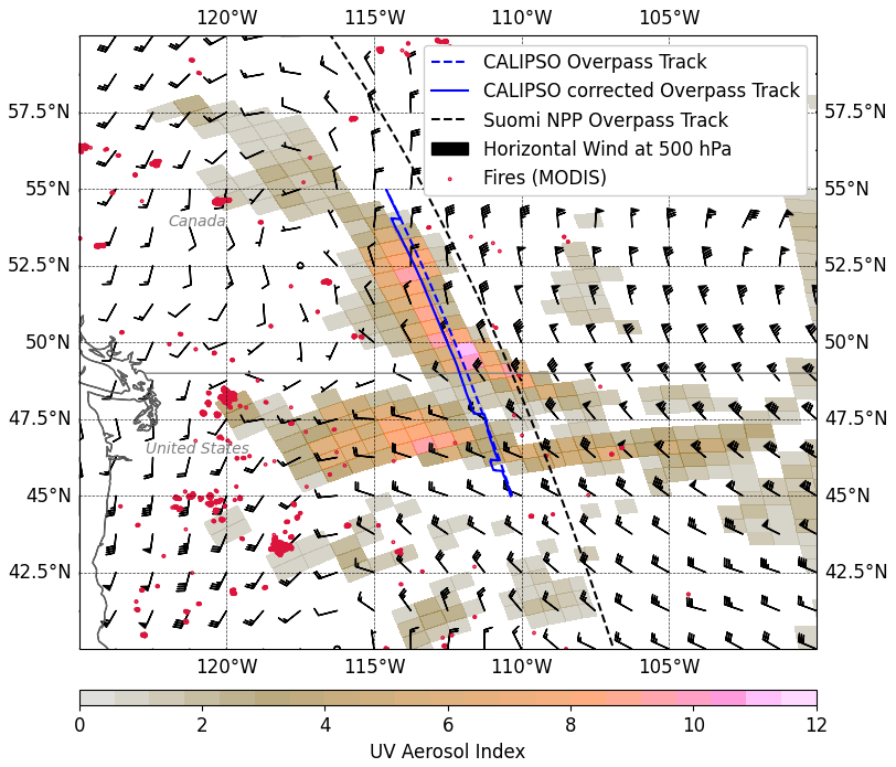
Figure 2 Map of wildfire smoke UVAI from the Carlton Complex Fire in Washington State and the Chukchuk Creek Fire in northeastern British Columbia, Canada on 18 July 2014: CALIPSO overpass between 20:33 and 20:35 UTC (blue dashed line). The Suomi-NPP overpass (black dashed line), is 53 min earlier (at 19:40 UTC) than the CALIPSO overpass. The theoretical plume location (upwind) at the time of the Suomi-NPP overpass is displayed (labeled as CALIPSO corrected Overpass Track, solid blue line). MODIS active fire hotspots betwen 16 and 18 July 2014 are shown by the red dots. Wind field in 500 hPa is depicted by wind barbs.

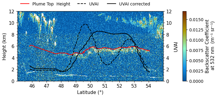
Figure 3 Latitude-height cross section of wildfire smoke in northeastern British Columbia, Canada on 18 July 2014: CALIOP attenuated backscatter coefficient at 532 nm and extracted values of the UV Aerosol Index (UVAI). The UVAI at the grid points along the original CALIPSO overpass track (dashed black line) and the “corrected” values of the UVAI at the windfield-corrected CALIPSO overpass track (solid black line) are displayed. Smoke plume top height is depicted by the red solid line.

2.3 Active Fire products

The Moderate Resolution Imaging Spectroradiometer (MODIS) instrument on board National Aeronautics and Space Administration (NASA)'s Earth Observing System (EOS) Aqua and Terra satellites has operationally detected active fires globally since 2000. The Aqua and Terra MODIS sensors are aging and nearing the end of their lives. Since 2017, the new generation moderate-resolution instrument called the Visible Infrared Imaging Radiometer Suite (VIIRS) on board the Suomi-NPP satellite provides continuity with MODIS (Li et al., 2018).

We obtain daily global active fire data from the MODIS MCD14ML product (Aqua and Terra combined) (Giglio et al., 2016) and the VIIRS 375 m active fire product VNP14IMGML (Schroeder et al., 2014), both available via the Fire Information for Resource Management System (FIRMS). The VNP14IMGML product is built on the modified active fire detection algorithm of the MODIS Collection 6 combined active fire product (Giglio et al., 2016), with modifications to separate fire pixels from background clear-land pixels (Li et al., 2018). A comparison between MODIS and VIIRS active fire data used in this study can be found in Li et al. (2018). The active fires detected in British Columbia and Washington State for the 18 July 2014 case are shown in Fig. 2.

2.4 Reference lidar observations at Leipzig, Germany

In 2022, a discrete fluorescence channel was incorporated into the Multiwavelength Atmospheric Raman Lidar for Temperature, Humidity, and Aerosol Profiling (MARTHA) system at the Leibniz Institute for Tropospheric Research (TROPOS) in Leipzig (Gast et al., 2025). The MARTHA system emits electromagnetic radiation at three wavelengths (355, 532, and 1064 nm) with an overall pulse energy of approximately 1.2 J at a repetition rate of 30 Hz. A detailed description of the system is provided in Mattis et al. (2002), Schmidt et al. (2013), Jimenez et al. (2019). The fluorescence channel added in the MARTHA lidar system is designed around a 44 nm wide interference filter centered at 466 nm (excitation wavelength: 355 nm). Further technical details on the setup can be found in Gast et al. (2025).

Generally, when excited by ultraviolet light, biogenic aerosol particles can be detected by measuring their laser-induced fluorescence emissions. Atmospheric fluorescent aerosols include biological particles such as pollen, viruses, fungi, bacteria, and spores, as well as non-biological compounds from biomass burning and fossil fuel combustion (Li et al., 2018). Mineral dust has also been found to produce a fluorescence signal, though it is relatively weak compared to that of biomass burning aerosols (Reichardt et al., 2018). The fluorescence spectrum varies depending on the type and composition of the aerosol. Because water does not fluoresce, fluorescent aerosols can be studied even in aerosol-cloud coexistence (Veselovskii et al., 2022a; Gast et al., 2025). However, an increase in relative humidity affects the fluorescence of water-soluble aerosol particles through hygroscopic growth, as well as that of water-insoluble particles due to the droplet lens effect. This complicates the retrieval of quantitative information about aerosol properties (Veselovskii et al., 2020).

The ability of certain aerosol particles to fluoresce may be expressed as the fluorescence capacity G_F

$$\begin{array}{}\text{(2)}& G_{\mathrm{F}}={\displaystyle \frac{{\mathit{\beta }}_{\mathrm{F}}}{{\mathit{\beta }}_{\mathrm{532}}}}\end{array}$$

which is the ratio of the fluorescence backscatter coefficient (β_F) to the elastic particle backscatter coefficient at 532 nm (β₅₃₂). The spectral fluorescence capacity with respect to the 355 nm wavelength $G_{\mathrm{F}}^{\mathrm{355}}$ can be expressed as

$$\begin{array}{}\text{(3)}& G_{\mathrm{F}}^{\mathrm{355}}={\displaystyle \frac{{\mathit{\beta }}_{\mathrm{F}}}{{\mathit{\beta }}_{\mathrm{355}}{d}_{\mathrm{IF}}}}\end{array}$$

where d_IF is the bandwidth (44 nm) of the interference filter in the fluorescence channel. Pollen and smoke exhibit significantly higher fluorescence capacity values compared to urban aerosol and mineral dust. Thus, when combined with information on the linear depolarization ratio, discrimination between smoke, mineral dust, pollen, and urban aerosol is possible (Veselovskii et al., 2021, 2022b).

Since 2022, profiles of the fluorescence backscatter coefficient have been obtained for a limited number of measurements, as the MARTHA lidar requires manual operation. Due to the broad bandwidth of the fluorescence channel and the low intensity of the fluorescence signal, measurements were only feasible during nighttime.

During daytime, when MARTHA measurements are unavailable, we use observations from the PortabLe Lidar sYstem with eXTended capabilities (Polly^XT) lidar (Engelmann et al., 2016) to interpret the air mass source estimate. Polly^XT is a Raman lidar that emits light at three wavelength channels. The technical setup of Polly^XT allows the measurement of the backscatter coefficient at 1064, 532, and 355 nm and the extinction coefficient at the two shorter wavelengths (532 and 355 nm). Additionally, Polly^XT is equipped with two polarization channels, providing measurements of the particle linear depolarization ratio at 532 and 355 nm (Baars et al., 2016). From these measurements, aerosol characterization is possible by comparing the respective extinction-to-backscatter ratio (lidar ratio) (Floutsi et al., 2023). A detailed description of the Polly lidar system can be found in Hofer et al. (2017), Jimenez et al. (2020).

3 Methodology: Air mass source – smoke attribution method TRAILS

In this approach, an air parcel arriving at a location of interest is considered to contain smoke aerosols if it either passed a smoke plume near an active wildfire hotspot or traveled through a smoke plume far from the original fire source. The likelihood of a detectable smoke aerosol signature increases with the air parcel's residence time in smoke-affected regions along its trajectory. Consequently, at a given altitude, a higher fraction of air parcels with long smoke plume residence times implies a greater probability of smoke aerosol presence. To quantify this relationship, we adapt the methodology of Radenz et al. (2021), computing the smoke occurrence fraction (SOF(z)) for each altitude bin z. This metric represents the percentage of smoke-contaminated air parcels at a given height, determined by their cumulative residence time within smoke plumes along their trajectories:

$$\begin{array}{}\text{(4)}& \mathrm{SOF}\left(z\right)={\displaystyle \frac{N_{\mathrm{smoke}}\left(z\right)}{N_{\mathrm{total}}\left(z\right)}}\times \mathrm{100}\mathit{\%}\end{array}$$

where z is the altitude bin, N_smoke(z) is the total number of smoke-identified air parcels at altitude z across all trajectories, $N_{\mathrm{total}}\left(z\right)=\mathrm{500}\times \mathrm{80}=\mathrm{40}\mathrm{000}$. For each altitude level, 500 air parcels are released, and their positions are tracked at 3 h intervals over 10 d (80 steps per trajectory), resulting in 40 000 potential parcel positions per level.

As in Radenz et al. (2021), we simulate the transport pathway of an air mass arriving at the study site using a Lagrangian particle dispersion model (LPDM), which provides a more realistic representation of turbulence and atmospheric mixing compared to conventional mean-wind trajectory methods like the Hybrid Single-Particle Lagrangian Integrated Trajectory model (HYSPLIT) (Stein et al., 2015). For this study, we utilize output from FLEXPART version 10.4 (Pisso et al., 2019), using meteorological data from the Global Forecast System (GFS) analysis at 1° horizontal resolution (National Centers for Environmental Prediction/National Weather Service/NOAA/U.S. Department of Commerce, 2000). The simulations use 500 air parcels per altitude level, with their positions recorded every 3 h along 10 d backward trajectories, at 500 m intervals from the surface up to 15 km.

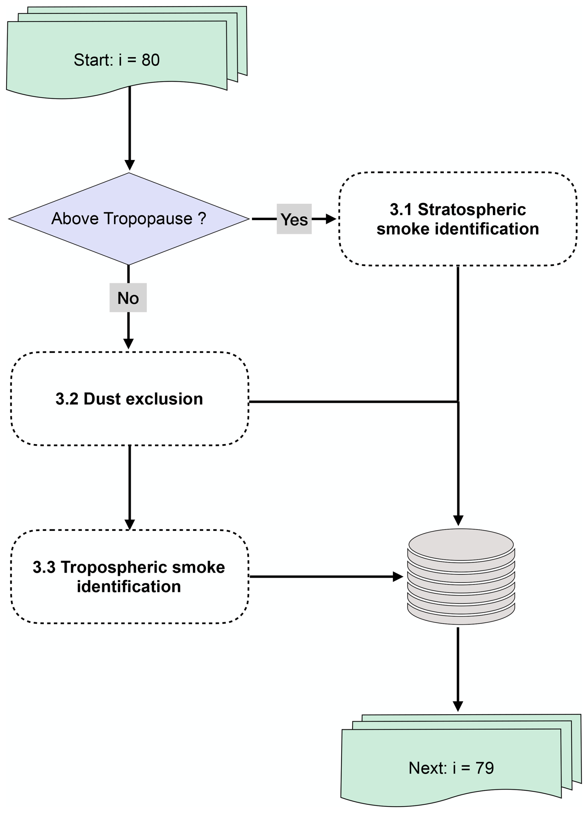
Figure 4 Simplified flowchart of the smoke attribution algorithm TRAILS. Ten-day backward trajectories from FLEXPART from the farthest point backward (time step i=80) are processed sequentially.

The identification of smoke-influenced air parcels from FLEXPART model output follows a multi-step classification process. Initial filtering excludes grid points affected by bright clouds by applying a minimum UVAI of 0.7 consistent with established approaches (Guan et al., 2010; Torres et al., 2007). The applied methodology to identify tropospheric smoke and to filter stratospheric smoke as well as dust is illustrated in Figs. 4 and 5, which are explained subsequently.

3.1 Stratospheric smoke identification

Attribution of smoke within the troposphere is the main goal of this study. Stratospheric smoke detection using the UVAI is treated as an experimental product, since the linear relationship between UVAI and aerosol properties is not generally valid for stratospheric plumes (Torres et al., 2020), particularly once they have aged (Guan et al., 2010). Smoke can be injected into the UTLS by intense pyroconvective events, where it can circulate globally and persist for several months to years (Ohneiser et al., 2022). Since our analysis is based on ten-day backward trajectories, stratospheric smoke plumes older than ten days cannot be attributed to their sources. Consequently, our approach is likely to miss aged or long-range transported smoke especially in the UTLS region. As shown in Fig. 4, the algorithm initializes at the air parcel position at step i=80 (corresponding to the 10th day backward in the trajectory). For each air parcel, FLEXPART provides the particle position and tropopause height (z_tropo) at 3 h time steps. If the air parcel's altitude (z_p) is located above the tropopause, potential stratospheric smoke influence is investigated (see Fig. 5). As an input, the daily maximum global UVAI field is used. Air parcels located above grid points where the UVAI exceeds the threshold UVAI_fresh=10 are classified as being influenced by fresh stratospheric smoke. While prior work has suggested that UVAI values greater than 15 indicate fresh stratospheric smoke (Torres et al., 2020; Peterson et al., 2021), our adopted threshold is comparatively lower. Further details on the sensitivity analysis and the discussion on the choice for this threshold are given in Appendix B. Once stratospheric smoke influence is detected, this information is retained and propagated along the trajectory. Subsequent air parcel positions are flagged as stratospheric if they are located above grid points where the UVAI exceeds the UVAI_aged threshold, applied to identify aged smoke plumes. For example, Guan et al. (2010) reported that plumes older than two days exhibited UVAI values between 5 and 10 at altitudes of 14–20 km. According to theoretical calculations describing the relationship between UVAI and AOD at a specified aerosol layer height (Torres et al., 2020), such plumes must have been optically thin (AOD <2).

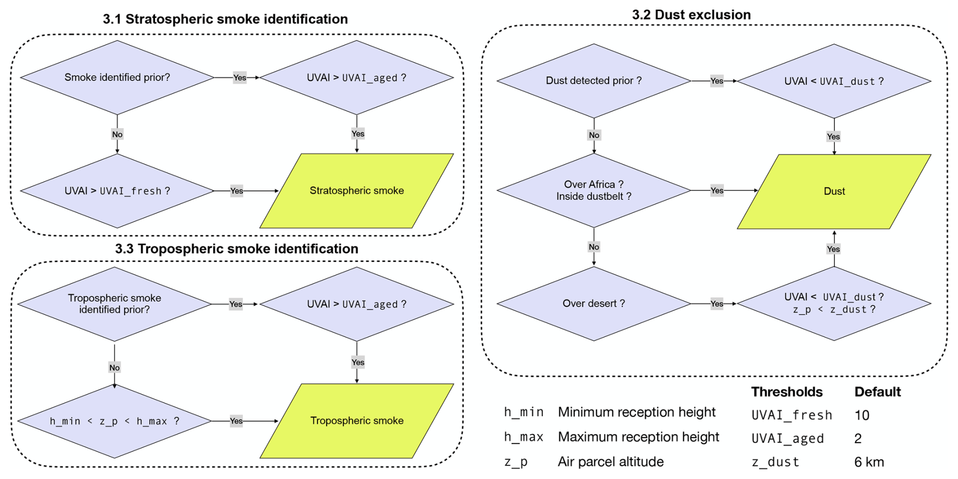
Figure 5 Overview of smoke and dust identification within TRAILS. Air parcels located within grid points where enhanced values of the UVAI are observed are assumed to be affected by smoke. For this, the classification involves comparing the air parcels altitude z_p with the location of the altitude of the tropopause and the theoretical plume height boundaries (h_min < z_p < h_max), estimated from the UVAI-plume height relationship. Different thresholds for dust (default UVAI_dust = 5) and stratospheric smoke identification (UVAI_fresh, UVAI_aged) can be chosen. The maximum dust plume altitude can be defined by z_dust.

To prevent unrealistic attribution, the algorithm imposes an upper altitude limit for stratospheric smoke identification. This limit is derived from the empirical relationship between UVAI and plume height established for tropospheric smoke (see Sect. 3.3 and Fig. 6). For a given UVAI value, the maximum reception height h_max,s is calculated. A stratospheric air parcel is only considered smoke-influenced if its altitude z_p lies between the tropopause and this dynamic altitude limit. In the default version of TRAILS we increase h_max,s by 4 km, which would equal a maximum altitude of 13.3 km for UVAI_fresh = 15 and 11.3 km for UVAI_fresh =10 (default version). However, grid points with UVAI values below 15 may either reflect an optically thin stratospheric smoke layer or an optically thick aerosol layer within the troposphere. Thus, we acknowledge that a complete separation between tropospheric and stratospheric smoke plumes cannot always be achieved. Moreover, stratospheric smoke might be mixed into the troposphere and therefore introduce another uncertainty in the smoke attribution. This limitation is particularly relevant because the decay phase of stratospheric smoke varies strongly between events. Gravitational settling is likely the dominant removal process, resulting in a slow and continuous decay of the smoke. Nevertheless, transport from the stratosphere to the troposphere can still occur during tropopause fold events (Breuninger et al., 2025; Haarig et al., 2026). These events, however, are rare and challenging to trace. Over the Arctic, a strong polar vortex may enhance vertical air mass exchange linked to the Brewer–Dobson circulation, facilitating downward transport of stratospheric smoke (Ohneiser et al., 2022). Furthermore, stratospheric smoke removal within the more isolated Southern Hemisphere (Ohneiser et al., 2022) might be more slow compared to the Northern Hemisphere, adding hemispheric variability to the detectability of aged smoke layers in the UTLS. Aged smoke can influence the evolution of cirrus clouds. Its subsequent removal by falling ice crystals further modifies the vertical distribution of smoke (Ansmann et al., 2025; Gast et al., 2025).

Taken together, these factors show that stratosphere–troposphere exchange processes further complicate smoke attribution. The UVAI-based identification of stratospheric smoke should therefore be interpreted with caution. We expect that our ten-day trajectory approach likely underestimates the occurrence, persistence, and vertical transport of stratospheric smoke signatures. Nonetheless, the focus of this study lies on tropospheric smoke attribution, and the final data product stores stratospheric- and tropospheric-affected air parcels separately. The attribution of stratospheric smoke therefore remains experimental, but it provides a practical means to minimize biases and to isolate tropospheric aerosol–UVAI relationships. A sensitivity analysis of the UVAI thresholds is presented in the Appendix.

3.2 Dust exclusion

While long-range transported dust is typically confined to the troposphere, deep convective systems can episodically inject it into the UTLS (Vernier et al., 2011). As our algorithm specifically targets tropospheric smoke plume detection, we omit a dedicated stratospheric dust identification to maintain simplicity and focus. For the tropospheric component of the analysis, potential dust influence must be excluded. Consequently, if the altitude (z_p) of the air parcel is located below the tropopause (see Fig.5), it is screened for dust influence. To mitigate false positives from dust, air parcels over Africa with UVAI > UVAI_cloud and z_p < z_tropo are categorically labeled as dust-influenced. This approach, however, also excludes African biomass burning aerosols and mixed dust–smoke scenarios. In practice, this means that all subsequent air parcel positions along a trajectory are excluded from smoke identification once the trajectory enters a dust source region. We acknowledge that this leads to an underestimation of smoke influence for trajectories that pass over Africa. However, for the scope and location of this study, which focus on smoke transported to Leipzig, Germany (51° N) from May to October 2023, this bias is minimized. The primary biomass burning seasons in Northern Hemisphere Africa typically occur from December to April (Roberts et al., 2009), outside our analysis period. Therefore, while the dust filter is coarse, its impact on the quantitative results for wildfire smoke arriving over Leipzig, Germany, is likely small. We opt for this conservative approach as it robustly increases the true positive rate for smoke identification from the dominant North American source region, which is the primary focus. Future applications of TRAILS in other regions or seasons may benefit from a more sophisticated dust-fire discrimination method.

Dust is identified when a trajectory passes either over Africa (defined by 35° S to 37° N, 20° W to 55° E) or within the global dust belt (30° S–10° N) (Prospero et al., 2002). As with stratospheric smoke, dust attribution is stored along the trajectory so that downstream positions can be consistently flagged as dust-influenced, even if they extend beyond Africa or the dust belt. Previous studies have shown that UVAI values exceeding 4 are indicative of elevated dust during severe dust storms (Asutosh et al., 2022; Kaskaoutis et al., 2008). In cases where dust was previously identified and the UVAI subsequently falls below the maximum dust threshold (UVAI_dust), the air parcel remains classified as dust-affected below an experimental altitude threshold (z_dust). While z_dust remains preliminary, its refinement lies beyond the scope of this study, which focuses primarily on tropospheric smoke identification. As a default, z_dust is set to 6 km (above mean sea level), representing the maximum dust layer altitude for extreme Saharan dust outbreaks near the west coast of Africa (Pu and Jin, 2021). Future work will address a more systematic evaluation of this parameter.

Dust storms outside the dust belt or Africa are also considered. For example, small-scale events in the Aralkum Desert, Kazakhstan, have been observed to produce UVAI values exceeding 3 (Xi et al., 2025). For such localized storms, dust is identified for air parcels located below an experimental altitude threshold (z_dust) above grid points with UVAI values lower than UVAI_dust. As input, we use the daily global mean UVAI field together with MODIS land surface classifications to identify deserts (category Barren) (Friedl et al., 2002). Once dust is identified along a trajectory, all subsequent air parcel positions are excluded from potential smoke attribution, ensuring that dust contamination does not bias smoke identification. This is particularly important given the spectral overlap between dust and smoke in UVAI, which often complicates attribution in mixed aerosol regions.

3.3 Tropospheric smoke identification

Air parcels affected by tropospheric smoke plumes are identified based on their location relative to grid points with enhanced UVAI values and their altitude. A new relationship between UVAI and plume height has been established for the Suomi-NPP UV Aerosol Index, extending previous work by Guan et al. (2010) on OMI-derived UVAI. As shown by Guan et al. (2010), UVAI exhibits a linear relationship with aerosol layer height for young tropospheric and stratospheric smoke plumes. Figure 6 confirms a pronounced linear dependence of UVAI on plume height for young tropospheric smoke in the Suomi-NPP UVAI product, with a statistically significant correlation (R²=0.50, p<0.001). Our analysis indicates that approximately half of the observed UVAI variability can be attributed to changes in plume altitude, with a standard error of 0.017.

The systematically lower UVAI values (UVAI < 7) observed for Russian smoke plumes compared to North American and Australian counterparts likely result from several interrelated factors. First, boreal forest fires in Russia typically burn at lower intensities than those in North America (Wooster and Zhang, 2004), with surface fires accounting for approximately 75 % of burned area in Siberia. In contrast, crown fires dominate the more intense North American forest fires. These differences are largely driven by divergent plant functional types between Siberian and North American boreal forests (Wirth, 2005). It has been shown that increased fire intensity enhances particle emission and coarse-mode aerosol production (Reid and Hobbs, 1998). Consequently, the lower UVAI for Russian plumes could result from differences in particle size distribution, composition, and resultant AOD. Peterson et al. (2025) reported lower pyroCb activity in Russia compared to North America, resulting in fewer high-altitude smoke injections. Over North America, storm systems from the Pacific Ocean provide the atmospheric instability and moisture necessary for pyroCb formation (Peterson et al., 2017). In contrast, South-East Siberia frequently experiences dry, anticyclonic conditions influenced by monsoon circulation (Damoah et al., 2004), which often do not fulfill the necessary ingredients for pyroCb development (Peterson et al., 2017). Consequently, Russian plumes remain predominantly in the mid-troposphere where UVAI sensitivity to height is reduced.

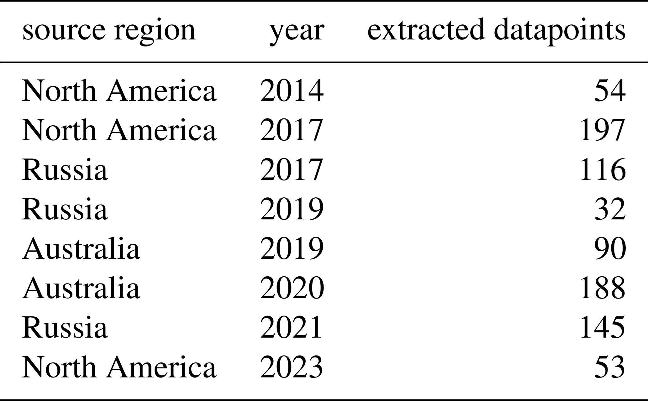
The spread in plume heights across all regions likely results from a combination of factors, including differences in satellite overpass times, variations in aerosol optical depth, and heterogeneity in smoke composition. Additionally, the potential presence of underlying cloud contamination due to the coarse spatial resolution of OMPS-NM (50 km × 50 km) is likely another source of uncertainty. As our empirical relationship (Eq. 5) does not explicitly account for this effect, cloud-contaminated pixels could bias the derived plume height upward. This potential positive height bias may partly offset the underestimation in plume height from optically thin or aged smoke plumes, which are expected to produce a weaker UVAI response for a given height (Torres et al., 2012; Jethva et al., 2018). However, as aerosol optical depth decreases, the sensitivity to enhanced scene reflectance also decreases (Jethva et al., 2018). We do not attempt to disentangle or explicitly correct for either effect. Consequently, the retrieved plume-height relationship is expected to be especially reliable for optically thick, young tropospheric smoke plumes over low-reflective underlying scenes (e.g. cloud-free conditions). It should be noted that our objective is not to retrieve exact layer heights but rather to constrain the horizontal and vertical extent within which smoke may occur. An overview of wildfire source regions and extracted data points for each year, serving as the basis for Fig. 6, is provided in Table 3.

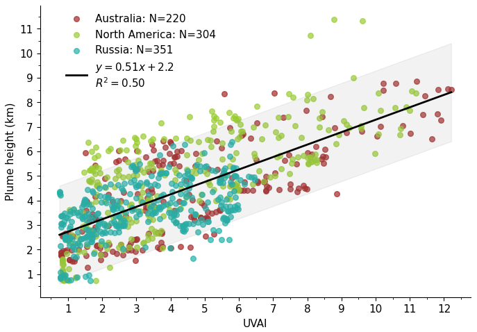
Figure 6 Scatterplot of OMPS-NM UV Aerosol Index versus CALIOP smoke plume height for fresh tropospheric smoke. Also annotated are the linear regression fit, number of scatterpoints (N) for each smoke affected region and the coefficient of determination (R²). The grey shaded area shows the lower and upper limits for the smoke identification using the FLEXPART output.

Table 3 Overview of extracted data point of young tropospheric smoke plumes per region and year of the fire season.

For air parcels near fires that do not meet stratospheric or dust conditions and reside below the tropopause (z_p < z_tropo), tropospheric smoke identification requires the parcel altitude to fall within theoretical plume height boundaries (h_min < z_p < h_max), estimated from the UVAI–plume height relationship as follows:

$$\begin{array}{}\text{(5)}& h=\mathrm{0.51}\cdot \text{UVAI}+\mathrm{2.2}\mathrm{km}\end{array}$$

from which the maximum and minimum reception heights $h_{\max ,\mathrm{t}}=h+\mathrm{2}$ km and $h_{\min ,\mathrm{t}}=h-\mathrm{1}$ km (default version) are derived.

This dynamic definition of plume height boundaries directly addresses the “reception height” problem highlighted in the introduction. Instead of assuming that air parcels only acquire smoke properties near the surface (e.g., within the PBL or below a fixed reception height of 2 km altitude), our method allows the reception height to be vertically dynamic and spatially variable. It is explicitly defined by the observed intensity of the UVAI and its corresponding estimated plume altitude. This represents a fundamental advancement over the previous tool introduced by Radenz et al. (2021), enabling the attribution of smoke influence for elevated plumes that have been injected directly into the free troposphere, thereby providing a more accurate and physically representative source attribution for wildfire emissions.

This criterion is applied under two key assumptions. First, continuous wildfire emissions near the source maintain stable UVAI–plume height relationships, despite temporal offsets between the Suomi-NPP overpass time and the FLEXPART air parcel positions. Second, we assume that smoke plumes within the troposphere will dilute if they are not lifted into the upper troposphere by processes such as WCBs within the first few days after emission. Consequently, we circumvent the challenge of directly identifying aged, diffuse tropospheric smoke. We argue that sustained high UVAI values in aged plumes originate from optically thick, condensed plumes that have been elevated into the UTLS. Therefore, we classify a plume as aged smoke if it is detected along an air parcel trajectory where smoke was previously identified. Similar to the method for aged stratospheric smoke, once a tropospheric smoke detection is made, it is retained and propagated along the calculated trajectory. Subsequent air parcel positions are then flagged as containing tropospheric smoke if they pass over grid points where the UVAI exceeds the predefined UVAI_aged threshold used to identify aged plumes. By propagating the detection along trajectories in this manner, the method inherently accounts for the advection and lofting of smoke over time. This approach ensures a realistic representation of slower atmospheric uplift mechanisms, such as those driven by WCBs. These processes typically require 2–4 d to transport smoke-laden air masses from the lower troposphere to the UTLS region, as demonstrated by Khaykin et al. (2025).

Additionally, if an air parcel is located above a grid cell in the daily one-degree averaged MODIS FRP grid and the cell exceeds the threshold of (FRP_thresh), the parcel is identified as smoke-influenced from the surface up to h_max. This condition ensures that air parcels positioned directly over a fire and with a height z_p below h_min are identified as smoke-influenced, provided the fire is sufficiently large and persistent to maintain burning over a daily period.

We set FRP_thresh = 30 MW based on detection reliability, not fire behaviour. This threshold sits at the upper end of the peak in fire detection across all world regions (Laurent et al., 2019) and well above the sensor's detection limit (9–11 MW (Roberts and Wooster, 2008)). Consequently, reaching 30 MW on average across a grid cell requires a robust and spatially consistent fire signal. This is different from the FRP level at which fire size stops growing, which Laurent et al. (2019) show varies widely by region (roughly 10 to 280 MW). Since our goal is to filter out unreliable low-intensity detections rather than to match a specific fire regime, a single global value based on detection statistics fits better than a region-specific one.

4 Results and Discussion

The 2023 wildfire season in Canada (late April to early October) was historically unprecedented, both in its intensity and hemispheric-scale impacts. Over 15.6 million ha of boreal forests, mixed-wood forests, and peatlands were burned across Alberta, British Columbia, Quebec, Ontario, and Saskatchewan. The combustion of these distinct vegetation types generated smoke plumes with complex aerosol compositions, which were subsequently transported across the Atlantic Ocean towards Europe (Filonchyk and Peterson, 2024). From mid-May to mid-July 2023, aerosol layers were frequently observed via lidar measurements over Leipzig (Gast et al., 2025). We will focus on two case studies during that period to evaluate the smoke attribution tool TRAILS with lidar observations.

4.1 29 May–2 June 2023: Biomass burning aerosol at Leipzig, Germany

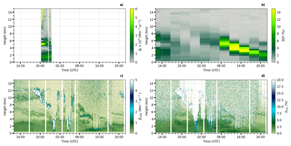
The period from 29 May to 2 June 2023 over Leipzig was characterized by the presence of extensive biomass burning aerosol layers. Figure 7 illustrates their temporal evolution, as captured by the complementary MARTHA (fluorescence, nightly) (panel a) and Polly^XT (continuous) (panels c–d) lidar systems. Smoke occurrence fractions retrieved from the airmass attribution tool are shown in panel (b). Several fluorescent aerosol layers were detected throughout the troposphere. These layers are partly visible in the Polly^XT measurements of the 1064 nm attenuated backscatter coefficient shown in panel (b), although they are most prominent at altitudes below 6 km. The evolution of cirrus clouds with ice virga between 7 to 12 km on the afternoons of 29 and 31 May can be recognized by increased values of the attenuated backscatter coefficient and the depolarization ratio, which are typical for irregularly shaped ice particles (panel c). Likely, ice nucleation was initiated at heights >10 km and at temperatures of below −50 °C according to model data from the ECMWF Integrated Forecast System (IFS). A detailed analysis of the fluorescence measurements from 29 May 2023, including potential smoke-cirrus interactions, is presented in Gast et al. (2025). For the aerosol layers below 6 km the depolarisation ratio in panel (d) shows values below 7 %. These values are in agreement with those found in aged tropospheric canadian smoke plumes (Ortiz-Amezcua et al., 2017). The signal-to-noise ratio in the Polly^XT measurements is lower during day, making aerosol features less distinct above 4 km.

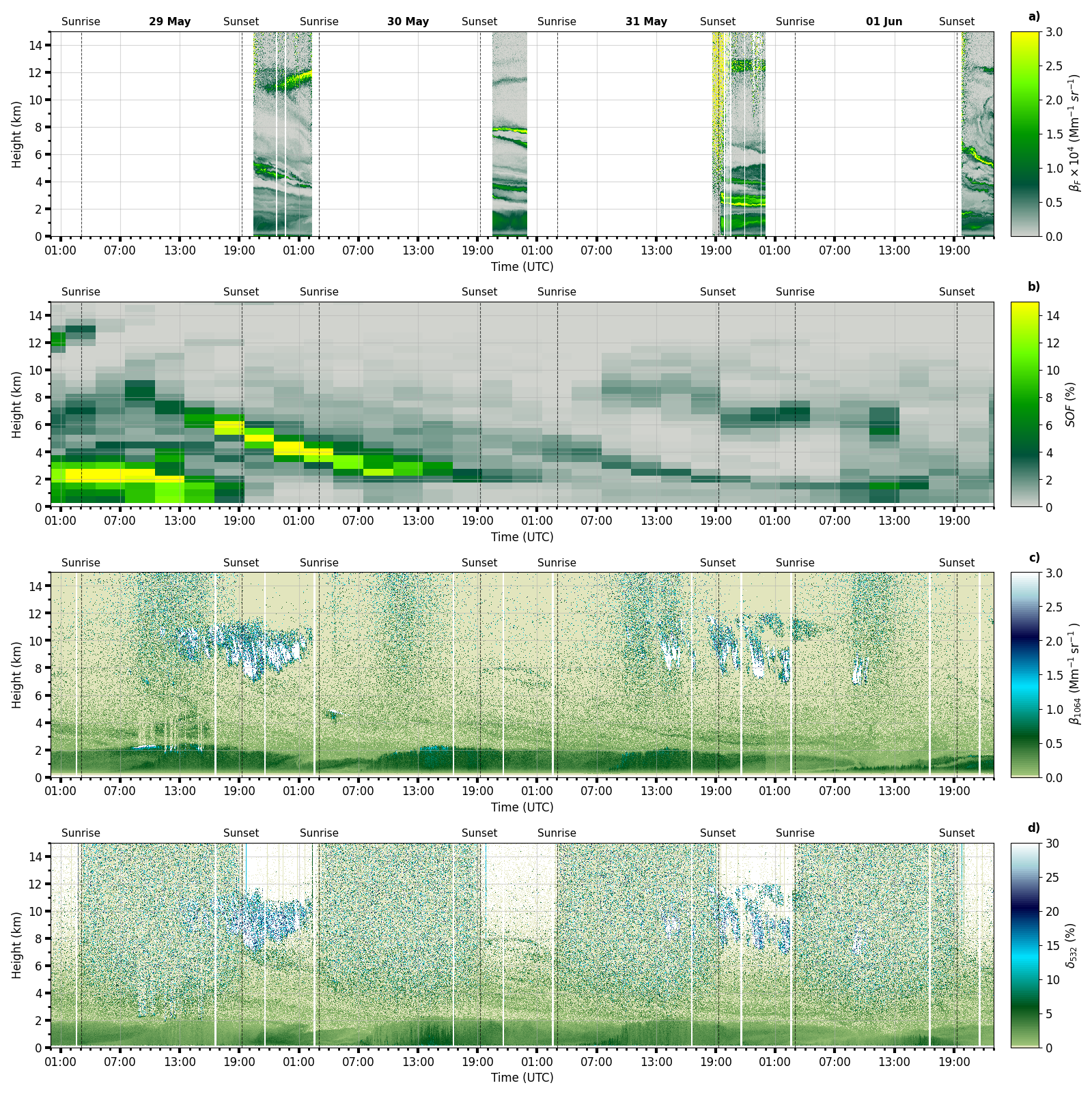
Figure 7 29 May–2 June 2023 Leipzig: (a) MARTHA fluorescence backscatter coefficient (β_F), (b) Smoke occurrence fraction (SOF), (c) Polly^XT backscatter coefficient at 1064 nm (β₁₀₆₄) and (d) Polly^XT depolarisation ratio at 532 nm (δ₅₃₂).

Layered aerosol features identified as smoke by our retrieval show enhanced SOF values exceeding 15 % on 29 and 30 May 2023. This stratified structure coincides with the altitudes of aerosol layers detected by both lidars. The observed wave-like patterns are consistent with the passage of a warm front, which transported smoke along tilted isentropic surfaces between approximately 4–8 km. Trajectory analysis indicates that smoke identified air parcels originated in the mid-troposphere (at around 5 km) over the western Atlantic. These air parcels were then lofted within the warm conveyor belt (WCB) of a mid-latitude cyclone located south of Iceland over the North Atlantic. Such frontal ascent provides a typical pathway for transporting polluted air and smoke from the lower to the upper troposphere (Eckhardt et al., 2004; Khaykin et al., 2025). From around 40° N, 60° W, the air parcels moved northward, ascending to about 7 km within one day before their trajectories turned anticyclonically over Western Europe. This transport pathway and its timescale (1 km d⁻¹) are characteristic of air mass ascent within warm conveyor belts (Eckhardt et al., 2004). The upper portion of the frontal zone arrived near 09:00 UTC on 29 May 2023, coinciding with observed enhancements in SOF near 8 km and the presence of cirrus clouds, which are typical of warm-frontal overrunning. The lower portion of the front passed the site around 03:00 UTC the following day. Subsequently, subsidence led to further downward mixing of the smoke layer. This subsidence is evident in the MARTHA lidar observations in Fig. 7a), which show a gradual descent of thin aerosol layers. The associated large-scale downward motion also suppressed cloud formation during the surface warm-front passage. The overall synoptic situation closely resembles conditions described by Evgenieva et al. (2025), featuring a stationary anticyclone over the North Atlantic that promoted large-scale descent through combined cold-air advection and negative vorticity advection.

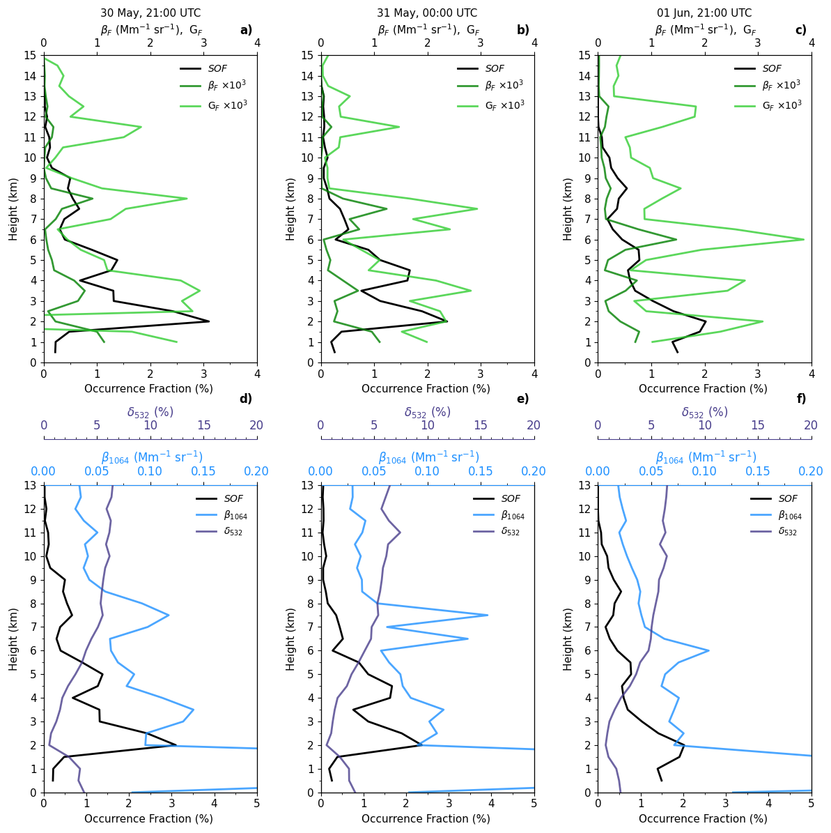
Figure 8 30 May 2023 at 21:00 UTC (a, d), 31 May 2023 at 00:00 UTC (b, e), and 1 June 2023 at 21:00 UTC (c, f): Smoke occurrence fraction (SOF) vs. MARTHA fluorescence backscatter (β_F) and capacity (G_F) (a–c), and compared to the Polly^XT particle backscatter coefficient at 1064 nm and volume linear depolarisation ratio at 532 nm (d–f).

Figure 8 shows MARTHA and Polly^XT lidar 1 h mean (centered at the full hour) vertical profiles between 30 May and 1 June 2023 averaged over 500 m height bins to match the resolution of the TRAILS output. The SOF is shown against the fluorescence backscatter coefficient together with the MARTHA fluorescence capacity (panels a–c) and against the Polly^XT elastic-backscatter coefficient at 1064 nm and depolarisation ratio at 532 nm in panels (d)–(f). Profiles at 21:00 UTC on 30 May 2023 (panels a and d), at 00:00 UTC during the night of 30–31 May 2023 (panels b and e), and at 21:00 UTC on 1 June 2023 (panels c and f) over Leipzig were selected, as they correspond to cloud-free periods where a reduction in fluorescence backscatter through effects such as fluorescence quenching or aerosol scavenging within cirrus clouds are negligible. Moreover, MARTHA lidar fluorescence measurements are only available during the night, with hourly mean profiles centered on the full hour (requiring at least 50 % data availability), whereas the SOF has a time resolution of 3 h (21:00, 00:00, 03:00 UTC, etc.). Consequently, only the profiles at 21:00 and 00:00 UTC can be used for evaluating the SOF against the fluorescence measurements.

The fluorescence measurements (particularly the fluorescence capacity G_F) reveal multiple elevated aerosol layers, with mean layer heights between 2–12 km. On 30 May at 21:00 UTC, three distinct layers were detected (3.5, 8, and 11 km height), splitting up into five during the night of the 30 to 31 May at 00:00 UTC. By 1 June at 21:00 UTC, these five layers were present again, with particularly high fluorescence capacity in the lower troposphere (up to 3.8 $\times {\mathrm{10}}^{-\mathrm{4}}$), consistent with previously reported values for wildfire smoke over Europe (Hu et al., 2022; Veselovskii et al., 2022b; Gast et al., 2025). In comparison, the Polly^XT backscatter coefficient profiles showed fewer and less distinct layers. For example, on 30 May only four broad layers were identified, with substantially weaker particle backscatter coefficients at 11 km. On 31 May, five layers were detected, but the UTLS layer remained faint. Overall, fluorescence lidar provides higher sensitivity to elevated aerosol layers, especially in the UTLS, whereas Polly^XT backscatter coefficient at 1064 nm captures the broader layer structure but struggles to resolve weak layers at high altitudes. This finding aligns with previous observations by Gast et al. (2025). In general, the particle depolarisation ratio increases steadily from 0.5 % at 2 km towards 6 % at 10 km. The observed increase in the depolarisation ratio with altitude indicates reduced condensation of water vapor, which suppresses the formation of a spherical coating on the aerosol particles in the drier upper troposphere, leading to more irregular shapes (Haarig et al., 2018; Ansmann et al., 2021).

The SOF profiles between 30 May at 21:00 UTC and 31 May at 00:00 UTC reveal four smoke layers (2–11 km height), with peak intensities decreasing from 3.4 % in the lower troposphere to about 1 % near 8 km. The detection of the highest layer required lowering the threshold to 0.1 %, indicating a reduced detection performance at these altitudes. Using our layer-matching procedure, three SOF layers (2.25, 7.5, and 10.5 km) correspond to layers in the G_F profiles, with an average altitude difference of −300 m and slightly larger thicknesses (+100 m). Layer thickness was determined by calculating the distance between the points where the peak intersects a specified reference level (50 % of the peaks prominence height). This requires predefining the peak threshold and peak prominence, which are summarized in Sect. 5. On 1 June at 21:00 UTC, however, fewer layers were detected with SOF: the UTLS layer at 12 km is missing, and two mid-tropospheric G_F layers (3.75 and 6.25 km) are merged into a single broader SOF layer at 5.25 km. Only the lower (1.75 km) and upper-tropospheric (8.25 km) layers showed good agreement with G_F. These results demonstrate that while SOF generally captures the main smoke structures and mean layer heights agree well with G_F profile, it tends to underestimate thin layers, particularly in the UTLS. This highlights the benefit of independent fluorescence measurements.

Interestingly, smoke-affected trajectories for detected layers in the SOF profiles originated from wildfires in British Columbia, Alberta, the Northwest Territories, and Saskatchewan between 21 and 23 May 2023. According to Beverly and Schroeder (2024), fires in Alberta that started in mid-May were mostly crown and surface fires caused by lightning. Burned area in May in Alberta was predominantly forested with conifer and mixedwood fuel. The dominant conifer fuel type reported is the C-2 Boreal Spruce fuel type of the Canadian Forest Fire Behaviour Prediction (FBP) System (Beverly and Schroeder, 2024). The C-2 Boreal Spruce is moderately well-stocked, with tree crowns extending nearly to the ground (Forestry Canada Fire Danger Group, 1992). It remains an open question, however, how the optical and microphysical properties of such aged smoke aerosols are influenced by this specific fuel type.

4.2 9–10 July 2023: Dust and Biomass burning aerosol at Leipzig, Germany

An example of wildfire smoke in the presence of mixed-phase clouds is shown in Fig. 9. Between 20:00 and 23:00 UTC on 9 July 2023, the fluorescence backscatter reveals an aerosol layer between 4 and 6 km altitude, also captured by the Polly^XT lidar. Prior to 20:00 UTC, a second aerosol layer is detected by the Polly^XT lidar between 10 and 12 km. Throughout the night, precipitating mixed-phase clouds developed in the vicinity of the smoke layers. Cirrus clouds (top height at around 12 km at temperatures $<-\mathrm{60}$ °C) are also visible, identified by elevated backscatter coefficients in panel (c) and relatively high depolarization ratios (>20 % – indicative of non-spherical ice crystals) in panel (d). By 23:30 UTC, attenuation in the lidar signal at 5 km suggests the development of liquid layers, with the mixed-phase cloud system reaching a top height of about 8 km (cloud-top temperature $\sim -\mathrm{30}$ °C). Precipitation onset was observed on 10 July at 00:00 UTC by the Parsivel2 disdrometer and lasted until 00:25 UTC. A second mixed-phase cloud produced precipitation between 04:15–04:40 and 05:00–05:20 UTC. These rain events are clearly visible in the Polly^XT volume depolarization ratio in panel (d), which increased to 10 %–15 % below 4 km at these times. Interestingly, after 06:00 UTC, enhanced particle backscatter reappeared between 4 and 6 km, with the layers appearing optically thicker than before precipitation. The temporal evolution of the SOF closely matches the lidar observations, supporting the interpretation of the aerosol layers as wildfire smoke. In particular, the correspondence of enhanced SOF values with the lower-tropospheric smoke layers after precipitation exemplifies the detection performance of our tool.

Figure 9 Same as in Fig. 7 at Leipzig on 9 to 10 July 2023.

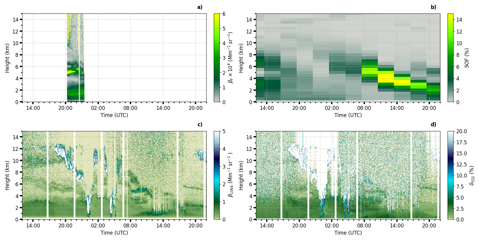
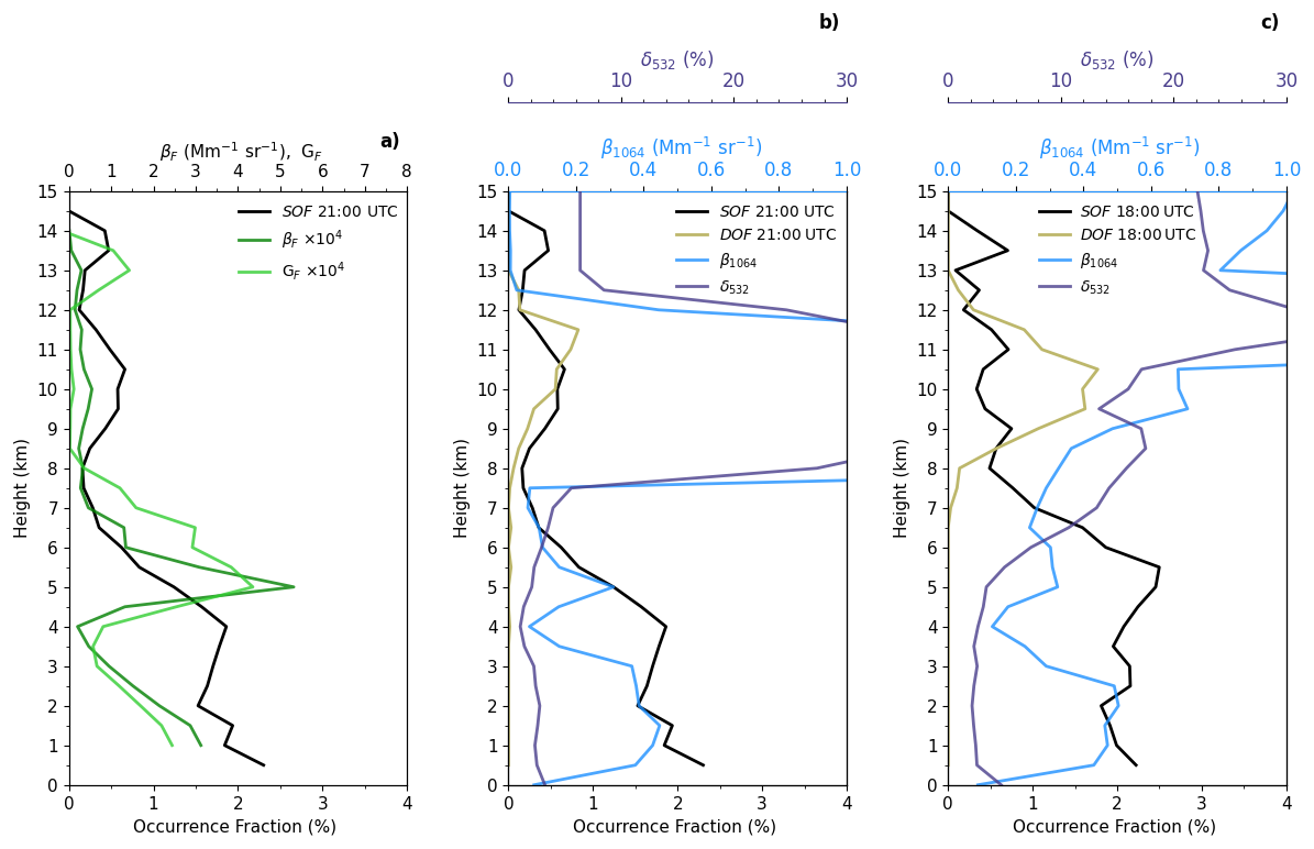
Figure 10 Leipzig on 9 July 2023: Same as Fig. 8 at 21:00 UTC (a–b). Additionally, the dust occurrence fraction (DOF) at 21:00 UTC is shown in (b). Panel (c) presents a comparison of the Polly^XT measurements with the SOF and DOF at 18:00 UTC .

Looking at the hourly averaged lidar profiles on 9 July 2023 at 21:00 UTC in Fig. 10a), the fluorescence lidar detects two fluorescent layers at 5.5 and 13 km. In contrast, the SOF profile identifies layers at 3.5, 10.25, and 13.75 km. In short, the SOF profile at 21:00 UTC does not include the layer at 5.5 km. However, in the SOF profile at 18:00 UTC (Fig. 10c), the SOF shows a peak at 5.5 km layer, illustrating that our tool does not always capture the time evolution of the layers precisely, possibly due to the 3 h time resolution. It is likely that the middle smoke layer at 5.5 km was mixed downwards between 18:00 and 21:00 UTC, such that the SOF layer at 3.5 km (peak at 4 km) at 21:00 UTC actually corresponds to the lidar-observed fluorescent layer at 5.5 km. Interestingly, the smoke layer between 4–6 km primarily originated from wildfires which occurred between 1–3 July 2023 in Northern Quebec (Nunavik), Canada, with a smaller fraction of trajectories passing through the Rocky Mountain Trench wildfire region. Both areas are characterized by boreal forests dominated by black spruce and pine species.

The SOF profile shows a distinct increase at a layer centered around 10.25 km at 21:00 UTC while the fluorescence capacity at this altitude remains weak. At 21:00 UTC between 8 to 12 km (at 18:00 UTC between 11 and 12 km), enhanced backscatter coefficient and particle depolarisation ratio (>30 %), indicate the presence of cirrus clouds. Enhanced Polly^XT depolarisation values (at 18:00 UTC: >15 % between 7 and 10.5 km indicate the presence of nonspherical particles like dust (Haarig et al., 2022). However, depolarisation ratios of biomass burning aerosol exceeding 15 % at 532 nm have also been previously observed in the UTLS region (Haarig et al., 2018; Hu et al., 2019). Ten-day back trajectories support the interpretation of dust presence: some trajectories arriving at 10 km originated near the Pinacate and Gran Desierto de Altar (Mexico), part of the larger Sonoran Desert system extending into the U.S. (Yuma Desert). Air parcels located below 5 km were tracked over grid points with UVAI values up to 5 and MODIS land cover classified as “Barren” (1° resolution). The resulting dust occurrence fraction (DOF) over Leipzig on 9–10 July 2023 is included in Fig. 10b and c. For both times, a dust layer was identified at 10 km with DOF >1.9 and DOF >3.5.

Taken together, these results demonstrate that the enhanced SOF at 10 km cannot be caused by false smoke attribution. Instead, the evidence points to either uncertainties in trajectory calculations or, more plausibly, the coexistence of dust and smoke in the same altitude range, i.e., a mixed dust–smoke layer at 10 km. This comparison demonstrates that relying on the SOF alone may lead to ambiguities in distinguishing smoke from dust. Incorporating measurements of the particle depolarisation ratio alongside the SOF therefore enhances the robustness of our tool, ensuring more reliable identification of aerosol type in complex scenes with coexisting smoke and dust layers.

5 Validation with MARTHA

We compare the smoke occurrence fraction (SOF) profiles with the fluorescence capacity (G_F) profiles rather than with fluorescence backscatter, as mineral dust may also fluoresce but typically exhibits a low fluorescence capacity. For dust, the maximum G_F is approximately $\mathrm{0.5}\times {\mathrm{10}}^{-\mathrm{4}}$, whereas for biomass burning smoke, the maximum G_F can be up to fifty times higher (Veselovskii et al., 2021, 2022b).

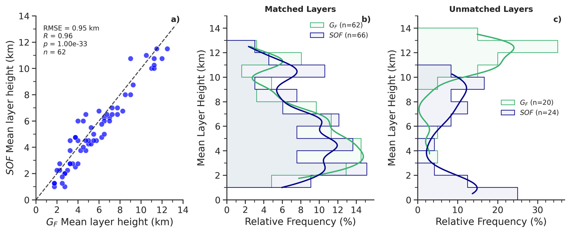
Figure 11 Correlation of matched mean layer heights of detected peaks in the profiles of smoke occurrence fraction (SOF) and lidar fluorescence capacity (G_F) (a). The number of matched G_F layers (n), as well as the RMSE, correlation coefficient, and p-value, are shown. Panels (b) and (c) display the relative frequency of matched and unmatched mean layer heights, respectively. The validation dataset comprises 23 profiles, of which layers were matched within a height tolerance of 2 km.

In general, we do not expect the intensity of the smoke occurrence fraction (SOF) to correlate directly with fluorescence capacity. Instead, the SOF serves as an indicator of the potential influence of wildfire smoke on an airmass, with larger values suggesting a greater likelihood of smoke contribution to the observed aerosol properties. The air parcel transport in FLEXPART is assumed to be broadly reasonable; however, the model setup for this study does not account for certain physical removal processes. Specifically, the AIRTRACER used to simulate smoke transport was configured without wet deposition parameterizations. Consequently, the removal of smoke aerosols through precipitation is not represented in our simulations. Furthermore, backward trajectory computations do not account for diabatic heating effects, which can alter vertical transport and lead to differences in layer heights, particularly in the UTLS region. Smoke self-lofting induced by diabatic heating may reach up to 1 km d⁻¹ (Ohneiser et al., 2023). Consequently, we expect systematic mismatches between layer heights of increased SOF and observed G_F layer heights in these regions.

The smoke detection tool TRAILS developed in this study is modular and relies on the synergy of several satellite products. Consequently, the accuracy of the retrieved smoke plume altitudes (reception heights) is affected by the uncertainties inherent in the input datasets as well as the thresholds applied. A sensitivity study on the influence of different thresholds is presented in the Appendix A. These uncertainties must be considered when interpreting SOF profiles in the context of independent observations. Even if the retrieved reception heights were assumed to be perfect, a long residence time, and thus a high SOF, would still represent a necessary but not sufficient condition for the aerosol load of an air parcel, as previously emphasized by Radenz et al. (2021). The fluorescence capacity itself may also be affected by environmental conditions, especially the presence of clouds or variations in relative humidity. An increase in relative humidity generally reduces the G_F signal (Veselovskii et al., 2021). Consequently, comparing SOF layer characteristics with layer characteristics of fluorescence measurements offers a more robust validation approach than comparing absolute signal intensities.

We compare the profiles of the SOF at matching times with profiles of the 1 h mean fluorescence capacity G_F. A total of 23 G_F profiles are available for validating the smoke detection tool performance. Using the scipy.find_peaks function by Virtanen et al. (2020) with specified detection parameters, we identified 82 fluorescence layers in the G_F profiles and 90 smoke layers in the SOF profiles. For G_F, layer detection required a threshold of $\mathrm{1}\times {\mathrm{10}}^{-\mathrm{4}}$, a peak prominence of $\mathrm{0.5}\times {\mathrm{10}}^{-\mathrm{4}}$, and a minimum peak width of 0.5 km. These thresholds follow Veselovskii et al. (2021), ensuring that the detected G_F layer peaks are well above the ones typical for dust. For SOF, we applied a threshold of 0.1 %, a peak prominence of 0.05 %, and a minimum peak width of 0.5 km. SOF parameters were optimized to maximize the matching efficiency between the datasets. Layer matching was performed by calculating the minimum height difference between detected layers within each profile, considering layers with a maximum height difference of 2 km as matches. A case study by Ohneiser et al. (2020) demonstrated that backward trajectory models can underestimate smoke layer altitudes by up to 2 km, primarily due to the omission of self-lofting processes. Therefore, a 2 km tolerance was selected as a conservative threshold to account for these biases, which are expected to be particularly relevant for smoke layers in the UTLS regions. The approach allows one-to-many matches, meaning that a single layer in one dataset can correspond to multiple layers in the other. This results in 62 matched layers, corresponding to a layer detection performance of 76 % relative to the total number of G_F layers.

As shown in Fig. 11a, the matched smoke layers (only the closest matches are shown) exhibit a strong positive correlation between mean and peak heights (R²=0.96), which is a consequence of the forced matching within the ±2 km tolerance window. The average mismatch between G_F and SOF mean layer heights is 0.95 km. For these matched layers, TRAILS systematically underestimates both mean and peak heights by about 0.4 km compared to the fluorescence observations ($t=\mathrm{3.590},p=\mathrm{0.0007}$, RMSE=0.95 km). We attribute the systematic low bias in the modeled heights to the combined uncertainties in UVAI-based plume height retrievals and the complexities of tropospheric transport, mixing, and removal processes along the 10 d trajectories.

The relative frequency distributions for all matched layers (Fig. 11b) illustrate the vertical structure agreement and discrepancy. Both SOF and G_F show a primary peak near 4 km, indicating good agreement in the lower troposphere. A secondary peak, however, reveals a systematic offset: it occurs at approximately 11.5 km for G_F but only around 10.5 km for SOF. This indicates an average underestimation of roughly 1 km by TRAILS for smoke layers in the upper troposphere and lower stratosphere (UTLS) region. This mean altitude difference of approximately 1–3 km for UTLS smoke layers implies an average ascent rate on the order of 0.1–0.4 km d⁻¹ over a typical smoke transport time of 7–9 d. This rate is well within the range of theoretical estimates for radiatively driven self-lofting of aged, optically thin smoke layers within the middle troposphere (Ohneiser et al., 2023).

The analysis of unmatched layers provides further insight. 85 % of the unmatched G_F layers are located at altitudes above 10 km. These likely correspond to smoke directly injected by pyroconvection, which was exceptionally frequent from May to August 2023 (Khaykin et al., 2025). Conversely, Fig. 11b) shows that most unmatched SOF layers reside between 5–10 km (50 %). These layers failed to match because the height difference between them and their potential G_F counterparts exceeded the 2 km tolerance. We hypothesize that many of these mid-level SOF layers correspond to the unmatched, higher-altitude G_F layers observed above 10 km. Moreover, 45.8 % of unmatched SOF layers are located below 5 km, indicating the smoke is frequently mixed into the boundary layer.

Taken together, these results indicate that the detection performance of TRAILS decreases for altitudes above 10 km. Since FLEXPART explicitly resolves synoptic-scale dynamical lifting (e.g., in WCBs), these height mismatches cannot be fully explained by resolved dynamics. The most consistent explanation for the systematic smoke layer height underestimation by the model in the UTLS is the lacking representation of post-injection smoke self-lofting through diabatic heating in the passive trajectory calculations of FLEXPART. The consequent vertical displacement moves the lidar-observed smoke layer outside the matching tolerance of the modeled TRAILS layer, providing an indirect observational signature of radiatively-driven ascent. For the 2023 Canadian wildfires, Khaykin et al. (2025) emphasized direct PyroCb injection as the dominant stratospheric pathway (between May–August 2023), noting the absence of large-scale, vortex-confined self-lofting. Our results align with this dominant pathway but also suggest the presence of a slower, more diffuse diabatic lofting process affecting smoke in the UTLS.

6 Conclusions

This study successfully extended the automated air mass source attribution tool of Radenz et al. (2021) to specifically identify wildfire smoke plumes and attribute their influence on an airmass. By integrating 10 d FLEXPART backward trajectories with a novel, multi-sensor satellite-based smoke detection algorithm, we developed a method to calculate a vertically resolved Smoke Occurrence Fraction (SOF). This metric quantifies the likelihood of smoke influence on an air parcel based on its residence time within smoke-affected regions, defined by Suomi-NPP OMPS UVAI observations and MODIS active fire data. The performance of the resulting SOF product was evaluated through detailed case studies and a statistical validation against independent, ground-based laser-induced fluorescence lidar measurements from the MARTHA system in Leipzig, Germany, during the record-breaking 2023 Canadian wildfire season. TRAILS identifies where and at what altitudes smoke is present, but does not automatically link these layers to their source fires. For the case studies presented, source attribution was performed by visually comparing the first smoke detection along trajectories with major active fire hotspots from MODIS/VIIRS.

The SOF profiles effectively captured the complex, multi-layered structure of long-range transported smoke, showing good agreement with the vertical distribution of aerosol layers observed by both fluorescence (MARTHA) and portable, automated multi-wavelength Raman (Polly^XT) lidars. A statistical comparison between detected SOF layers and fluorescent aerosol layers (G_F) revealed a high layer detection performance of 76 %. On average, the SOF-derived layer heights were slightly underestimated by approximately 0.4 km, with the discrepancy increasing to roughly 1 km for layers in the upper troposphere and lower stratosphere (UTLS). This systematic height mismatch provides indirect observational evidence for diabatic self-lofting, a process not represented in the air-tracer trajectory calculations of FLEXPART. The inferred ascent rate of 0.2–0.4 km d⁻¹ for UTLS layers is consistent with theoretical estimates for aged, optically thin smoke, offering a new observational constraint on this process. Therefore, the systematic height underestimation in the UTLS by TRAILS itself provides indirect observational evidence of diabatic lofting processes, offering a novel constraint on post-injection smoke ascent that is otherwise difficult to observe directly.

A key innovation of this work was the establishment of a new, statistically significant linear relationship between OMPS-NM UVAI values and smoke plume height for fresh tropospheric smoke. This relationship was derived by collocating Suomi-NPP OMPS-NM observations with independent, vertically resolved smoke plume heights retrieved from CALIOP lidar measurements aboard the CALIPSO satellite, thereby building upon the work of Guan et al. (2010). This relationship, alongside specific thresholds for identifying stratospheric smoke and for filtering out dust and cloudy scenes, formed the core of our modular smoke identification logic. In contrast to Radenz et al. (2021), who assumed air parcels only acquire smoke properties near the surface (e.g., within the PBL or below a fixed 2 km altitude), our method allows the reception height to be vertically dynamic and spatially variable. This represents a fundamental advancement over the previous tool introduced by Radenz et al. (2021), enabling the attribution of smoke influence for elevated plumes that have been injected directly into the free troposphere, thereby providing a more accurate and physically representative source attribution for wildfire emissions. The UVAI-plume height relationship (Eq. 5) was derived primarily from North American, Russian, and Australian smoke plumes (Fig. 6, Table 3). Its applicability to other fire types (e.g., agricultural burning) or regions with different aerosol composition remains to be validated.

The case study from 9–10 July 2023 demonstrated the TRAILS tool's capability to identify smoke layers even in the presence of complex cloud systems and mixed aerosol types. The combination of SOF with lidar depolarization ratios proved particularly valuable for distinguishing between pure smoke and dusty layers, highlighting the importance of independent lidar observations in conjunction with the SOF for unambiguous aerosol typing.

A key limitation of TRAILS in its current form is that it provides smoke layer detection but not automated source attribution. While the case studies include visual verification linking detected smoke to major fire hotspots (e.g., British Columbia, Alberta, Quebec), this step remains manual and qualitative. The tool does not yet automatically determine which specific fires contributed to an observed smoke layer, nor does it quantify the relative contribution from multiple potential source regions.

In conclusion, TRAILS provides a valuable, observationally constrained method for the time-height-resolved identification of wildfire smoke. When combined with lidar observations, especially depolarization ratios for aerosol typing, the SOF offers a valuable framework for interpreting aerosol layer origins and evolution. Consequently, TRAILS can help disentangle the effects of smoke aerosols from other INP and CCN sources, particularly at sites lacking of advanced fluorescence lidars. By delivering continuous, automated estimates of smoke influence, this tool can enhance investigations of aerosol-cloud interactions and the long-range transport of biomass burning aerosols.

From a technical perspective, the TRAILS algorithm is computationally efficient and modular. The daily processing of global satellite data and 10 d backward trajectories for multiple altitude levels can be automated for operational use. Its design allows for straightforward integration of new satellite datasets and adaptation to different geographic regions or aerosol types, such as volcanic plumes or dust storms. The implementation of the TRAILS framework thus represents an important step toward improved source attribution and quantification of smoke events. Future developments could integrate TRAILS with the source apportionment approach of Radenz et al. (2021) to assign an observed SOF signal to its likely source region. Furthermore, associating SOF values with forecasts from chemical transport models, such as those from the Copernicus Atmosphere Monitoring Service (Peuch et al., 2022), could improve estimates of smoke plume composition. Looking ahead, future work will focus on several key directions to advance the TRAILS framework and its scientific applications. First, we will apply TRAILS to biomass burning events across the Southern Hemisphere, including the Australian bushfires of 2019–2020 and recent observations from New Zealand. This extension will test the method's robustness under different meteorological regimes and fire characteristics and will be particularly valuable for studies focusing on biomass burning smoke over the Southern Ocean. Automating the fire source attribution step in TRAILS represents a key next step. By identifying where trajectories pass below a reception height threshold over active fire pixels, the tool would not only detect smoke layers but also trace them back to their specific fire sources, transforming TRAILS from a smoke detection tool into a complete source attribution system.

Appendix A: Recommended configuration and sensitivity study

TRAILS utilizes a range of data products and thresholds to identify wildfire-smoke-influenced air parcels from FLEXPART backward trajectories. The default configuration values, input data, and thresholds are summarized in Table A1. The default configuration (version 1) represents a balanced choice for general applications. However, parameter adjustments may optimize performance for specific use cases.

Table A2 provides an overview of the different configuration settings. All version contain the default input settings except when they are additionally specified in the table. Versions were created to test the sensitivity towards stratospheric smoke detection by varying the thresholds UVAI_fresh (2–3), tropospheric and stratospheric smoke detection by changing the reception height h_max,t (4–5) and h_max,s (6–7). In the following, the influence of changing these default thresholds is investigated.

Torres (2019)Friedl et al. (2002)Peterson et al. (2021)Guan et al. (2010)Asutosh et al. (2022)Pu and Jin (2021)Laurent et al. (2019)Prospero et al. (2002)

Table A1 Overview of the selected input parameters for the default version and respective references.

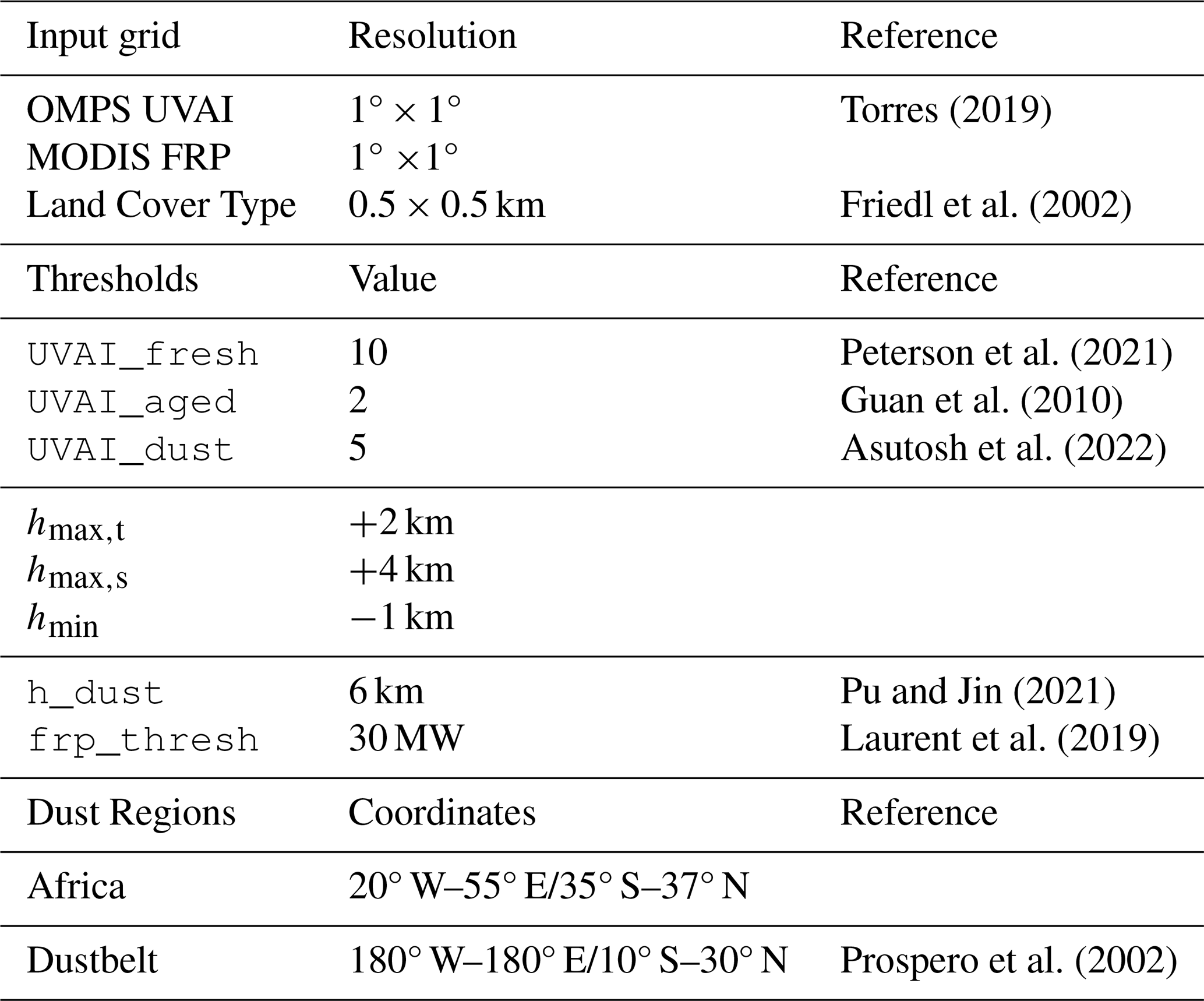
Table A2 Overview of processing versions used to determine optimal parameters. Versions 2–3 test UVAI_fresh threshold sensitivity; versions 4–5 test h_max,t sensitivity; versions 6–7 test h_max,s sensitivity.

Appendix B: Stratospheric smoke identification threshold

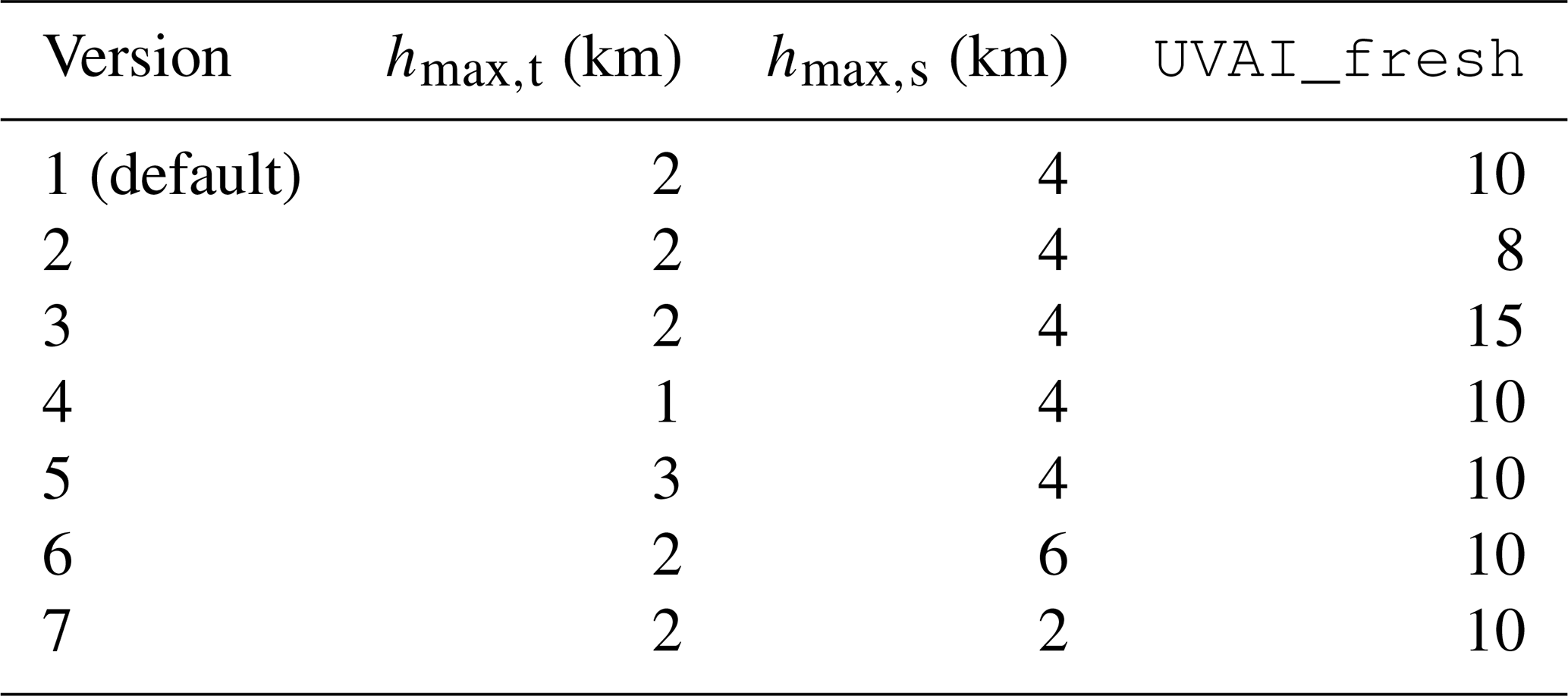
Figure B1a shows sensitivity in layer counts between mean layer heights (bin size = 2 km) derived from the smoke occurrence fraction (SOF) and those detected in the fluorescence capacity (G_F) observations. Positive values indicate that SOF overestimates the number of layers relative to G_F for a given mean layer height, whereas negative values indicate underestimation.

The impact of variations of UVAI threshold values is explored by modifying it in the following ways: A UVAI threshold of 10 for fresh stratospheric smoke identification is applied for the default version (V1). According to Torres et al. (2020), this threshold captures stratospheric smoke plumes with optical properties consistent with organic aerosol components and an AOD of approximately 1 (for sensors operating at 388 nm). Consequently, increasing the threshold excludes optically thinner smoke plumes, while lowering it includes more optically thinner plumes. Lowering the UVAI threshold to a value of 8 (V2) shows that the tool slightly overestimates layer occurrence compared to the default version, particularly above 6 km. This overestimation is remarkably reduced when the threshold is increased to 15, as TRAILS selectively identifies only optically thick elevated smoke plumes.

Differences between versions 1–2 become more apparent in geometrical mean layer thickness, as shown in Fig. B2a. Fluorescence observations (dashed grey line) show a tri-modal distribution in layer thickness with maxima at approximately 3.5, 5.5, and 7.5 km. At these peaks, layers are thickest (1.25–1.75 km), indicating frequent smoke layer occurrence. The minima between peaks likely reflect regions with fewer detected layers rather than consistently thinner smoke, as layer counts decrease at these intermediate altitudes (see Fig. B1a). Above 10 km, layers are consistently thinner (1 km). Below 4 km, TRAILS maintains similar mean layer thickness of 1.25 km at 2.5 km for versions 1–2, for version 15 layer thickness increases about 0.5 km. This indicates, that the number of thin layer below 4 km is reduced when lowering the UVAI_fresh threshold, because layer occurrence in this latitude range is reduced as well. Between 4–8 km–where the fluorescence distribution shows secondary maxima–layers are typically 1–1.25 km thick. TRAILS shows only a single broad peak in this range, indicating limited ability to resolve individual layers. Lowering the UVAI_fresh threshold increases mean layer thickness and narrows the distribution, suggesting reduced layer separation. Notably, UTLS thickness (8–12 km) remains consistent across all versions, supporting the hypothesis of frequent smoke mixing from the UTLS into the lower troposphere. In summary, modifying the stratospheric smoke identification threshold (UVAI_fresh) affects layer occurrence throughout the troposphere, as evidenced by variations in both layer counts and thickness between versions 1–3. While mean signal intensity shows minimal variation across these versions (and is therefore not shown), the changes in layer properties suggest downward mixing of UTLS air masses. This interpretation aligns with recent observations by Haarig et al. (2025), who documented smoke transport via tropopause folds and identified this as a key removal mechanism for stratospheric smoke during Northern Hemispheric summer. The sensitivity of our detection algorithm to these vertical transport processes validates its utility for studying cross-tropopause aerosol dynamics.

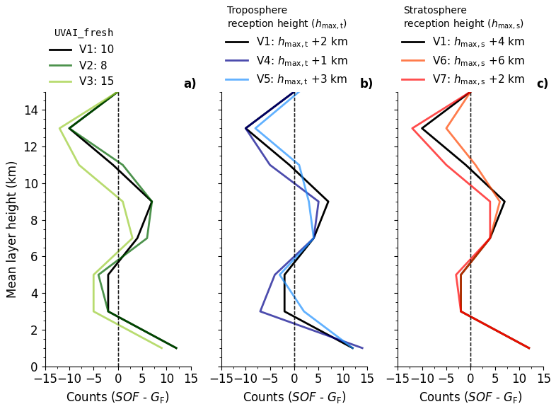
Figure B1 Layer count difference in between mean layer heights (bin size = 2 km) estimated using the smoke occurrence fraction (SOF) and fluorescence capacity (G_F) observations. Positive values indicate SOF overestimates layer counts relative to G_F, while negative values indicate underestimation. Number of matched layer (n) is displayed for each version (V) and the black line denotes the default version (V1). Detailed parameter specifications for different versions are provided in Table A2. Columns show variations in: (a) threshold values for stratospheric smoke identification (UVAI_fresh), (b) reception height threshold for tropospheric smoke identification (h_max,t), (c) reception height threshold for stratospheric smoke identification (h_max,s).

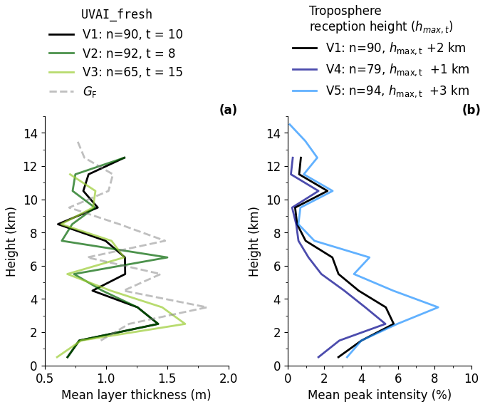
Figure B2 Vertical profiles of smoke layer properties: (a) Mean layer thickness for different UVAI_fresh thresholds (versions 1–3) compared to the fluorescence observations G_F (dashed line). (b) Mean SOF intensity for different tropospheric reception heights (versions 1, 4–5). Data are binned at 1 km vertical resolution.

Appendix C: Reception height maximum for tropospheric smoke

Figure B1b shows the tool's sensitivity to changes in the reception height threshold for tropospheric smoke identification. Both decreasing and increasing the reception height alter the number of detectable layers throughout the troposphere. This demonstrates the tool's high sensitivity to this parameter. A lower threshold corresponds to a stricter height tolerance for smoke identification. Consequently, decreasing h_max,t reduces the number of trajectories passing through this height region, and vice versa. This is also reflected in Fig. B2b, which shows that with increasing h_max,t, the mean intensity of the SOF signal increases, as more air parcel positions fall within the expanded height range considered for smoke identification. Physically, a more relaxed height range could include greater variability in AOD, plume height, and chemical composition (e.g., single-scattering albedo), all of which influence the UVAI. Furthermore, temporal offsets between the air parcel positions and the daily gridded UVAI measurements may be partially balanced by a broader height criterion. The selection of an optimal threshold h_max,t represents a balance between sensitivity and specificity. A stricter threshold improves specificity by reducing false positives but may exclude valid smoke layers affected by vertical dispersion or uncertainties in trajectory height. Conversely, a relaxed threshold increases sensitivity but may introduce uncertainty in source attribution by including aerosols from different origins.

Appendix D: Reception height maximum for stratospheric smoke

Modifying the stratospheric reception height threshold (h_max,s) primarily influences layer detection in the UTLS region, though smaller changes in layer counts extend down to 3 km (Fig. B1). Increasing h_max,s reduces layer count underestimation in the UTLS. It should be noted that layer thickness affects mean height calculations: thinner layers yield mean heights closer to their peak altitudes than thicker layers. Consequently, while total layer counts may remain constant, their vertical distribution can shift. Layer thickness remains remarkably consistent across all versions (and is therefore not shown), indicating that h_max,s primarily influences layer occurrence and SOF signal intensity rather than layer geometry. Mean SOF intensity shows minimal variation between version 1 (default) and version 6 ($h_{\max ,\mathrm{s}}=+\mathrm{6}\mathrm{km}$), suggesting the default threshold ($h_{\max ,\mathrm{s}}=+\mathrm{4}\mathrm{km}$) is adequate. For version 7 ($h_{\max ,\mathrm{s}}=+\mathrm{2}\mathrm{km}$), mean SOF intensity between 9.5–11.5 km decreases to near 0 %, approximately 2 % lower than versions 1 and 6. These intensity differences are confined to this narrow altitude range and are therefore not shown separately.