Assessment of an updated polar stratospheric cloud parameterisation for the UK Earth System Model (UKESM1.1) within the UK Met Office Unified Model (v13.9) using CALIOP and MLS observations

Accurately representing polar stratospheric clouds (PSCs) in global Chemistry-Climate Models and Earth System Models is important as they play a key role in springtime ozone depletion in polar regions by activating both chlorine and bromine species through heterogeneous reactions and denitrifying the stratosphere. Here, we present and evaluate an updated PSC parameterisation scheme implemented in the UK Earth System Model (UKESM1.1). The scheme includes the kinetic formation of nitric acid trihydrate (NAT) particles, the formation of supercooled ternary solution (STS) droplets assuming thermodynamic equilibrium, and accounts for ice and sulphate aerosols. To evaluate the new scheme, we compare modelled PSC production with satellite observations from the Cloud-Aerosol and Lidar with Orthogonal Polarization (CALIOP) instrument and model concentrations of gas-phase nitric acid, water vapour, and ozone concentrations with observations from the Aura Microwave Limb Sounder (MLS) instrument for the extended 2008 Antarctic and 2009/2010 Arctic winters. In comparison with the current, simpler scheme, the updated parameterisation increases both the range of PSC types that form and the seasonal variability, resulting in better agreement with CALIOP observations. However, there is still a gap in the model's ability to simulate ice PSCs with the full range of optical properties observed by CALIOP. The new scheme also slows the growth of NAT particles and enables nitric acid partitioning between gas, liquid, and solid phases, leading to improved agreement with gas-phase nitric acid MLS observations, although a substantial low-bias is still present in all model simulations. However, there is comparatively little impact on stratospheric ozone, with the exception near the edge of the polar vortex where the new scheme improves comparisons with MLS observations.

1 Introduction

Stratospheric ozone absorbs incoming solar radiation and its depletion leads to cooling of the polar stratosphere, influencing atmospheric circulation and surface climate (Randel and Wu, 1999; Polvani et al., 2011). Polar stratospheric clouds (PSCs) play a critical role in driving ozone depletion and shaping polar stratospheric chemistry. Heterogeneous reactions on the surfaces of PSCs convert reservoir chlorine and bromine species into active species during the polar winter, when the absence of solar radiation allows stratospheric temperatures to drop below the thresholds for PSC formation (Solomon et al., 1986; Tritscher et al., 2021). Once sunlight returns in spring, these active species participate in catalytic cycles that efficiently destroy ozone (O₃), resulting in rapid O₃ depletion (Molina and Molina, 1987). The threshold temperature for PSC formation depends on the composition of the PSC particles. Crystalline nitric acid trihydrate (NAT) are solid particles consisting of nitric acid (HNO₃) and water (H₂O) with formation temperatures of below T_NAT ∼ 195 K under normal stratospheric ambient conditions at 20 km. Supercooled ternary solution (STS) droplets grow through the uptake of HNO₃ on the background sulphate aerosols as temperatures decrease. Under normal stratospheric ambient conditions (i.e., 50 hPa with HNO₃ ∼ 10 ppb and H₂O ∼ 5 ppm), the typical temperature that HNO₃ rapidly condenses onto background sulphate aerosols is 191 K (although HNO₃ still condenses slowly on the background aerosols at higher temperatures if vapour pressures are high enough). Water ice particles form at the coldest temperatures of below T_ice ∼ 188 K (Koop et al., 2000; Engel et al., 2013).

Particle composition also influences PSC surface reactivity (Carslaw et al., 1997). For many heterogeneous reactions occurring below T_NAT, liquid droplets (e.g., STS) are comparable to, or more effective than, solid NAT and ice particles in activating chlorine based on reactivity per unit surface area (Ravishankara and Hanson, 1996). Peter and Grooß (2012) showed that chlorine activation rates of NAT could only compete with the chlorine activation rates of STS in high number density “mother clouds” that form downstream of ice clouds (Fueglistaler et al., 2002). Reaction rates on liquid binary H₂SO₄-H₂O aerosol particles also reach substantial values before NAT formation, indicating that chlorine activation is mainly driven by liquid heterogeneous chemistry. However, large solid ice and NAT particles sediment from the stratosphere into the upper troposphere, causing stratospheric denitrification and dehydration. Removal of reactive nitrogen limits the amount of nitrogen available to deactivate chlorine and prolongs periods of O₃ depletion (Toon et al., 1986). This effect is especially important in the Arctic, where temperatures are comparably higher and denitrification can result in greater ozone loss (Chipperfield and Pyle, 1998). In Antarctica, chlorine and bromine activation, combined with an increase in stratospheric chlorine loading due to anthropogenic release of chlorofluorocarbons, has resulted in severe springtime O₃ depletion in recent decades, forming a region of anomalously low total column ozone values referred to as the Antarctic ozone hole (Cicerone et al., 1974; Farman et al., 1985). This has significantly affected Southern hemisphere circulation and climate (Orr et al., 2008; Previdi and Polvani, 2014; Polvani et al., 2018).

To accurately simulate stratospheric ozone depletion, PSC parameterisation schemes in global Chemistry-Climate Models (CCMs) and Earth System Models (ESMs) must represent PSC formation and associated ozone-loss chemistry. However, the complexity of the PSC schemes in these models varies. For example, the SOCOL (SOlar Climate Ozone Links) model uses a relatively simplistic approach that assumes thermodynamic equilibrium between the PSC particles and gas phases, instantaneously forming PSCs when saturation vapour pressure is reached (Steiner et al., 2021). This requires assumptions about the particle size distribution, either number density or radius. By contrast, models such as EMAC (ECHAM5/MESSy Atmospheric chemistry model), ICON-ART (ICOsahedral Nonhydrostatic modelling framework and its Aerosol and Reactive Trace gases extension), and SD-WACCM-4.0/CARMA (Community Aerosol and Radiation Model for Atmospheres coupled to the Whole Atmosphere Community Climate Model with Specified Dynamics) use more complex methods to capture deviations from equilibrium conditions by simulating the growth and evaporation of particles, enabling a wider range of particle sizes to be represented (Kirner et al., 2011; Zhu et al., 2015; Weimer et al., 2021).

The UK Earth System Model (UKESM1.1) uses a relatively simple approach for PSC formation, accounting only for NAT, sulphate aerosols, and ice (Dennison et al., 2019). NAT particles are nucleated assuming thermodynamic equilibrium based on Hanson and Mauersberger (1988) and are assumed to have a fixed radius of 1.0 µm. Sulphate aerosols are included as a prescribed surface area density (SAD), and there is no mechanism for the formation of STS droplets (Sellar et al., 2019; Archibald et al., 2020). Ice particles are formed using the cloud microphysics scheme (Wilson and Ballard, 1999), but are assumed to have a fixed radius of 10 µm when calculating the SAD for heterogeneous chemistry. While the exact mechanisms of NAT nucleation are still not fully understood, the growth of NAT particles occurs over hours to days (Voigt et al., 2005), and are not in equilibrium when they grow to larger sizes (Carslaw et al., 2002). Therefore, the inability of this scheme to simulate NAT outside of equilibrium conditions and to form STS particles limits the capability of UKESM1.1 to represent all PSC particle types and their evolution over the PSC season, hindering its ability to accurately simulate stratospheric ozone depletion, including projections of future ozone recovery and associated climate impacts (Austin et al., 2003; Eyring et al., 2006, 2013; Zeng et al., 2022).

PSCs are observed with satellite measurements (Pitts et al., 2013; Spang et al., 2018), ground-based lidar (Snels et al., 2019) and airborne and balloon-borne in situ observations (Fahey et al., 2001; Voigt et al., 2003). Ground-based lidars provide measurements with high temporal resolution and enhanced signal-to-noise ratios of many variables, but their effectiveness can be limited by tropospheric cloudiness (Tesche et al., 2021). Airborne and balloon-borne in situ measurements offer detailed observations of trace gases and aerosols, including measurements of size and number concentration, but have limited temporal and spatial coverage. Satellite-based measurements such as the Cloud-Aerosol Lidar with Orthogonal Polarization (CALIOP) onboard the Cloud-Aerosol Lidar and Infrared Pathfinder Satellite Observations (CALIPSO), which operated from June 2006 until August 2023, use the depolarization ratio to infer the particle shape and concentration, enabling distinction between liquid and solid particles (Pitts et al., 2013). Given its excellent temporal and spatial coverage and ability to differentiate PSC types, CALIOP provides a robust benchmarking dataset to evaluate PSC parameterisations. Additionally, the Microwave Limb Sounder (MLS) instrument on board the Aura Satellite flew in formation with CALIPSO in the A-Train constellation until 2018 (Stephens et al., 2002), providing nearly coincident measurements of atmospheric gas variables, such as HNO₃, H₂O, and O₃ concentrations by observing passive thermal emissions on the millimetre and sub-millimetre wave length scale (Waters et al., 2006).

In this study, we address the limitations in the representation of NAT and STS particles in UKESM1.1 by replacing its current, simple representation of these particles with the more sophisticated representation employed in ICON-ART (Weimer et al., 2021). This approach kinetically forms NAT particles and thermodynamically forms STS particles, making it more interactive and physically based. We evaluate the performance of this new scheme relative to the current scheme by comparing modelled PSCs with CALIOP PSC observations during the 2008 Antarctic and 2009/2010 Arctic winters (Pitts et al., 2011, 2018). Comparing over both Arctic and Antarctic PSC seasons enables evaluation of the new parameterisation under the different dynamical conditions of the northern and southern polar vortices. For the Antarctic winter, we additionally investigate how the updated scheme affects the temporal evolution of PSCs and gas-phase HNO₃ and O₃ concentrations with a comparison against MLS measurements. Through these analyses, we assess how the new scheme alters UKESM1.1 PSC composition diversity and seasonal progression, while identifying remaining limitations and possible future model developments.

2 Models, Data, and Methods

2.1 Model Descriptions

2.1.1 UKESM1.1

UKESM version 1 (UKESM1.1) is a state-of-the-art Earth system model that is built around the global climate model HadGEM3-GC3.1, which is composed of the Unified Model (UM) atmosphere model, NEMO ocean model, and CICE sea ice model (Sellar et al., 2019; Mulcahy et al., 2023). Here we use version 13.9 of the UM, with a resolution of 1.875° longitude by 1.25° latitude and 85 vertical levels extending to 85 km (N96L85). Aerosols and trace gas chemistry are simulated using the stratospheric-tropospheric (Strat-Trop) configuration of the United Kingdom Chemistry and Aerosol (UKCA) model (Archibald et al., 2020), which includes v8.0 of the two-moment modal aerosol microphysics module GLOMAP-mode (Mann et al., 2010; Dhomse et al., 2014; Mulcahy et al., 2020). Strat-Trop employs 84 species and accounts for 299 reactions, including additional heterogeneous bromine reactions and updated uptake coefficients on aerosols and solid-phase PSCs implemented in UKESM1.1 (for more details, see Dennison et al., 2019).

In the original PSC parametrisation used by UKESM1.1, NAT is calculated following Chipperfield (1999), assuming thermodynamic equilibrium with gas-phase HNO₃ and H₂O. NAT is formed every time step when the partial pressure of HNO₃, $p_{{\text{HNO}}_{\text{3}}}$, exceeds the saturation vapour pressure of HNO₃ over NAT, $p_{{\text{HNO}}_{\text{3}}}^{\text{NAT}}$, calculated using the relationship defined in Hanson and Mauersberger (1988):

$$\begin{array}{}\text{(1)}& {\log }_{\mathrm{10}}\left(p_{{\text{HNO}}_{\mathrm{3}}}^{\text{NAT}}\right)=a_{\text{NAT}}\left(T\right)\times {\log }_{\mathrm{10}}\left(p_{{\text{H}}_{\mathrm{2}}\text{O}}\right)+b_{\text{NAT}}\left(T\right),\end{array}$$

where T is the temperature, $p_{{\text{H}}_{\mathrm{2}}\text{O}}$ is the partial pressure of H₂O, and

$$\begin{array}{}\text{(2)}& {\displaystyle }{a}_{\text{NAT}}\left(T\right)=-\mathrm{2.7836}-\mathrm{0.00088}\left(T\right),\text{(3)}& {\displaystyle }{b}_{\text{NAT}}\left(T\right)=\mathrm{38.9855}-{\displaystyle \frac{\mathrm{11397.0}}{T}}+\mathrm{0.009179}\left(T\right).\end{array}$$

This is only valid for the temperature range 180 K < T < 200 K. For temperatures below 180 K, $p_{{\text{HNO}}_{\text{3}}}^{\text{NAT}}$ is calculated with T = 180 K. All NAT particles are assumed to have a fixed-value radius, r_NAT, of 1.0 µm. Denitrification is prescribed based on Chipperfield (1999) with two different sedimentation velocities: one for pure NAT (0.46 mm s⁻¹) and one for mixed ice/NAT (17 mm s⁻¹) (Morgenstern et al., 2009).

Ice abundance is taken from the UM microphysics scheme which calculates the mass mixing ratio of ice using a single-moment scheme (Wilson and Ballard, 1999). The mass mixing ratio is then converted to a SAD by assuming a radius, r_ice, of 10.0 µm. STS formation is not explicitly included; instead, the effect of liquid droplets is accounted for with a prescribed SAD climatology from 1850–2014 prepared for the CMIP6 model intercomparison (Sellar et al., 2019; Archibald et al., 2020) Consequently, heterogeneous reaction rates are therefore calculated based on uptake on ice, NAT, and sulphate aerosols.

2.1.2 Updated PSC parameterisation

In the updated PSC scheme, the nucleation, growth, and evaporation of NAT particles is parameterised based on the analytic expression described in Carslaw et al. (2002). This is the same scheme implemented in ICON-ART, which was developed based on version 2.1 of ICON-ART (Schröter et al., 2018) and included in the published version 2025.04 (Hoshyaripour et al., 2026). Here, the time-dependent diffusive growth of the radius of a NAT particle, r_NAT, is estimated by:

$$\begin{array}{}\text{(4)}& {\displaystyle \frac{\mathrm{d}{r}_{\text{NAT}}}{\mathrm{d}t}}={\displaystyle \frac{G}{r_{\text{NAT}}}},\end{array}$$

where t is time, and G is the surface growth factor computed using:

$$\begin{array}{}\text{(5)}& G={\displaystyle \frac{D_{{\text{HNO}}_{\mathrm{3}}}^{*}{M}_{\text{NAT}}}{{\mathit{\rho }}_{\text{NAT}}RT}}(p_{{\text{HNO}}_{\mathrm{3}}}-p_{{\text{HNO}}_{\mathrm{3}}}^{\text{NAT}}),\end{array}$$

where M_NAT is the molar mass of NAT, ρ_NAT its density, and R the universal gas constant. $D_{{\text{HNO}}_{\mathrm{3}}}^{*}$ denotes the diffusion coefficient of HNO₃ in air, accounting for non-continuum mass transfer effects of particles comparable in size to the mean free path and is computed using:

$$\begin{array}{}\text{(6)}& D_{{\text{HNO}}_{\mathrm{3}}}^{*}={\displaystyle \frac{D_{{\text{HNO}}_{\mathrm{3}}}}{\mathrm{1}+\mathrm{4}{D}_{{\text{HNO}}_{\mathrm{3}}}/\left({\stackrel{\mathrm{‾}}{c}}_{{\text{HNO}}_{\mathrm{3}}}{r}_{\text{NAT}}\right)}},\end{array}$$

where $D_{{\text{HNO}}_{\mathrm{3}}}$ is the diffusion coefficient of HNO₃ in air, and ${\stackrel{\mathrm{‾}}{c}}_{{\text{HNO}}_{\mathrm{3}}}$ is the mean molecular speed of HNO₃.

To determine the new r_NAT at each time step as a result of growth or evaporation, Eq. (4) is integrated over time, t, which gives:

$$\begin{array}{}\text{(7)}& r_{\text{NAT}}^{\mathrm{2}}(t+\mathrm{\Delta }t)=r_{\text{NAT}}^{\mathrm{2}}\left(t\right)+\mathrm{2}G\mathrm{\Delta }t,\end{array}$$

where Δt is the chemistry time step (equal to 1 h in UKESM1.1).

To implement the kinetic NAT formulation in UKESM1.1, size bins with fixed radii are defined according to van den Broek et al. (2004). Nine bins, each with an average radius r_NAT,b and number density limit, n_NAT,lim,b, where b is the bin index, span radii from 0.1 to 22.5 µm, based on the observed range and distribution (Fahey et al., 2001). This results in a total maximum NAT number density limit, $n_{\text{NAT,max}}={\sum }_b{n}_{\text{NAT,lim},b}$. In this study a range of values for n_NAT,max are used to assess the sensitivity to NAT number density. Regardless of the choice of value for n_NAT,max, NAT initially nucleates in the smallest bin (r_NAT of 0.1 µm) with a number density of $\mathrm{1.5}\times {\mathrm{10}}^{-\mathrm{5}}$ cm⁻³ when $p_{{\text{HNO}}_{\mathrm{3}}}>p_{{\text{HNO}}_{\mathrm{3}}}^{\text{NAT}}$ (see Eq. 1) with a 3 K temperature threshold applied in line with similar NAT parameterisations to account for the supersaturation required for NAT formation (Grooß et al., 2002; Kirner et al., 2011). The condition thus becomes:

$$\begin{array}{}\text{(8)}& p_{{\text{HNO}}_{\mathrm{3}}}>p_{{\text{HNO}}_{\mathrm{3}}}^{\text{NAT}}(T+\mathrm{3}\text{K})\end{array}$$

The change in particle radius within each size bin is calculated sequentially from the smallest to the largest bin using Eq. (4) and the bin-specific growth factor G_b following Eq. (5). Changes in radius are immediately converted to changes in number density, n_NAT,b, by conserving mass, ensuring all particles in a bin have the same size. If n_NAT,b exceeds its limit n_NAT,lim,b, excess mass is transferred to the next larger bin. Evaporation occurs when $p_{{\text{HNO}}_{\mathrm{3}}}<p_{{\text{HNO}}_{\mathrm{3}}}^{\text{NAT}}$, making G_b negative in Eq. (5). At T>220 K, particles fully evaporate. Each size bin is treated as a separate tracer and NAT sedimentation is determined interactively, with the fall velocity calculated for each bin based on Stokes' law.

In the updated PSC scheme, STS droplets are formed by calculating the volume density of the sulphate aerosols or STS, V_STS, based on the uptake of HNO₃ and H₂O on aqueous sulphuric acid aerosols using the thermodynamic scheme documented in Carslaw et al. (1995). At temperatures above which HNO₃ uptake is negligible, V_STS corresponds to binary sulphate aerosols; as temperatures decrease, HNO₃ uptake increases and V_STS corresponds to ternary solution droplets. V_STS is then converted to a SAD, S_STS, for heterogeneous chemistry using the relationship described in Grainger et al. (1995):

$$\begin{array}{}\text{(9)}& S_{\text{STS}}=a_{\text{SV}}(V_{\text{STS}}{)}^{b_{\text{SV}}},\end{array}$$

where a_SV=6.068 and b_SV=0.671 based on the empirical parameter fitting (Hervig and Deshler, 1998). The effective radius of the STS particles, r_STS, used when calculating the optical properties, is then determined by:

$$\begin{array}{}\text{(10)}& r_{\text{STS}}={\displaystyle \frac{\mathrm{3}{V}_{\text{STS}}}{S_{\text{STS}}}}.\end{array}$$

To implement the new STS scheme in UKESM1.1, the concentration of aqueous sulphuric acid aerosols is provided each timestep from the interactive GLOMAP aerosol microphysical module (Mann et al., 2010; Dhomse et al., 2014; Mulcahy et al., 2020) and is used to calculate V_STS. Note that the STS routine is called before the NAT routine in UKCA. This means that when temperatures fall below T_STS, HNO₃ uptake on sulphate aerosols is calculated first. The formation, growth, or evaporation of NAT is then calculated (from Eqs. 8 and 5) based on the remaining gas-phase HNO₃.

The new PSC scheme still computes ice PSCs using the UM microphysics scheme, but the conversion from mass mixing ratio to SAD has been modified. Previously, ice mass mixing ratio was converted to a SAD assuming a fixed radius (r_ice=10 µm). With this assumption, the ice number density, n_ice, doesn't exceed 0.01 cm⁻³, and the resulting SAD remains below 2.5 µm² cm⁻³ for the periods analysed in this study. Although observations of ice PSC size distributions are limited, these values are relatively low compared to other PSC schemes (Zhu et al., 2017; Tritscher et al., 2019; Weimer et al., 2021). Therefore, following the approach of ICON-ART, in the updated PSC scheme the ice SAD is instead calculated assuming a fixed value for n_ice (Weimer, 2019). However, although ICON-ART uses n_ice=0.25 cm⁻³, in this study we examine a range of n_ice values to assess the sensitivity of the results to this. For example, using higher n_ice values produce smaller ice particles with larger surface area densities.

With a prescribed n_ice, stratospheric r_ice is calculated as follows:

$$\begin{array}{}\text{(11)}& r_{\text{ice}}={\displaystyle \frac{\mathrm{1}}{\mathrm{2}}}\sqrt[\mathrm{3}]{{\displaystyle \frac{m_{\text{ice}}}{\mathrm{130}}}},\end{array}$$

where m_ice is the mass of ice particles, defined as

$$\begin{array}{}\text{(12)}& m_{\text{ice}}={\displaystyle \frac{\mathit{\rho }{W}_{\text{ice}}}{n_{\text{ice}}}},\end{array}$$

with W_ice the water mass mixing ratio of cloud ice and ρ the air density (Doms et al., 2011).

2.2 Observations

CALIOP was a dual-wavelength, polarization-sensitive lidar that observed profiles of the parallel and perpendicular components of the backscatter coefficients (β_⟂ and β_∥, respectively) at 532 nm and total backscatter at 1064 nm from mid-June 2006–August 2023 (Pitts et al., 2018). In this study, we use the CALIPSO lidar level 2 PSC mask version 2.0 (v2) which has a horizontal resolution of 5 km and vertical resolution of 180 m, and considers only nighttime measurements. This dataset was derived using the CALIOP v2 PSC Classification Algorithm (Pitts et al., 2018). For PSC detection, only the 532 nm backscatter coefficient measurements are used. The molecular number density (calculated using temperature and pressure fields from Modern-Era Retrospective analysis for Research and Applications, version 2 (Gelaro et al., 2017) reanalysis) is used in the theoretical calculation described in Hostetler et al. (2006) to determine the molecular backscatter, β_mol, which is then used to compute the 532 nm attenuated scattering ratio, R₅₃₂:

$$\begin{array}{}\text{(13)}& R_{\text{532}}={\displaystyle \frac{{\mathit{\beta }}_{\parallel }+{\mathit{\beta }}_{⟂}}{{\mathit{\beta }}_{\text{mol}}}}.\end{array}$$

PSCs are identified as statistical outliers in β_⟂ or R₅₃₂. Daily threshold values of β_⟂ and R₅₃₂ are defined as the median plus one median absolute deviation (${\mathit{\beta }}_{⟂,\text{threshold}}$ and R_threshold, respectively). A PSC occurrence is then defined as exceeding either background threshold by at least the measurement uncertainty, σ:

$$\begin{array}{}\text{(14)}& {\displaystyle }{\mathit{\beta }}_{⟂}>{\mathit{\beta }}_{⟂,\text{threshold}}+\mathit{\sigma }\left({\mathit{\beta }}_{⟂}\right),\text{(15)}& {\displaystyle }{R}_{\text{532}}>R_{\text{threshold}}+\mathit{\sigma }\left(R_{\text{532}}\right).\end{array}$$

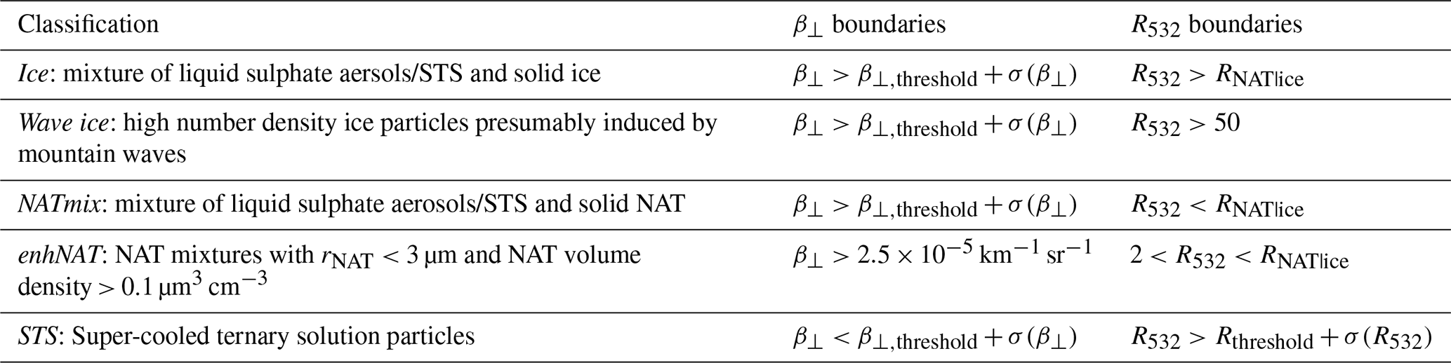
where σ(β_⟂) and σ(R₅₃₂) are computed using the noise-scale factor approach of Liu et al. (2006) as described for CALIOP by Hostetler et al. (2006). PSCs with β_⟂ exceeding the background threshold are assumed to contain non-spherical (i.e., solid) particles. The solid-containing PSCs are further classified as either liquid-NAT mixtures (NATmix), enhanced NAT mixtures with r_NAT ≲ 3 µm and NAT volume density ≳ 1.0 µm³ cm⁻³ (enhNAT), ice, or high-number-density ice that forms in mountain waves (wave ice). enhNAT is separated from NATmix using boundaries of R₅₃₂>2 and ${\mathit{\beta }}_{⟂}>\mathrm{2.5}\times {\mathrm{10}}^{-\mathrm{5}}$ km⁻¹ sr⁻¹, determined from empirical comparisons between CALIOP and MIPAS observations with and without the NAT band formed heterogeneously from wave ice (Höpfner et al., 2006). Since v2 of the CALIOP classification algorithm (Pitts et al., 2018), the R₅₃₂ boundary separating enhNAT and NATmix from ice, R_NAT|ice, is derived from relationships based on MLS HNO₃ and H₂O concentrations computed for weekly “cloud-free” conditions in equivalent latitude bands and potential temperature layers. The R_NAT|ice for a specific CALIOP observation is then estimated by finding the appropriate equivalent latitude band and potential temperature and using the corresponding R_NAT|ice value for the week. The wave ice boundary, R₅₃₂>50, is from the v1 CALIOP classification algorithm (Pitts et al., 2011). PSCs below ${\mathit{\beta }}_{⟂,\text{threshold}}$, but above R_threshold are classified as STS, with no maximum for R₅₃₂. These classification boundaries are summarised in Table 1, though it is important to note that they are not all-inclusive, i.e., enhNAT might not capture all NAT mixture PSCs that are heterogeneously nucleated downstream of wave ice PSCs. For more details on the CALIOP v2 PSC Classification Algorithm, see Pitts et al. (2018).

Table 1 Boundaries in R₅₃₂ and β_⟂ values used to classify PSC observations using CALIOP v2 PSC classification. Thresholds ${\mathit{\beta }}_{⟂,\text{threshold}}$ and R_threshold are the median plus one median absolute deviation, and σ(β_⟂) and σ(R₅₃₂) are the measurement uncertainties of β_⟂ and R₅₃₂ respectively. The boundary between ice and both NATmix and enhNAT, R_NAT|ice, is calculated dynamically.

The Aura MLS passively measures microwave thermal emissions from the ground to 90 km to retrieve profiles of about 20 trace gases and cloud properties. It takes measurements at wavelengths in the millimetre to sub-millimetre range from the limb of Earth's atmosphere from 82° S to 82° N every 25 s (Waters et al., 2006). In this study, model outputs are compared with MLS level 2 data (Livesey et al., 2006) for HNO₃, H₂O, and O₃. The MLS HNO₃ product is derived from the 240 GHz retrievals at pressures ≥ 22 hPa and 190 GHz retrievals for lower pressures, with a vertical resolution of 3–4 km in the region of interest. The MLS H₂O product is derived from the 190 GHz retrievals with a vertical resolution of 1.3–3.6 km in the region of interest. The MLS O₃ product uses the 240 GHz radiances and has a vertical resolution of 2.5 km.

2.3 Methodology

2.3.1 Comparing to observations

To compare PSCs simulated by UKESM1.1 with those observed by CALIOP, the particle size distributions from the model are used to calculate optical parameters offline as they would be observed by the satellite, i.e. β_⟂ and β_∥. The same classification algorithm used for CALIOP optical properties can then be applied to the model outputs. Comparing directly with the satellite optical properties is preferable to using the CALIOP SAD product derived from these properties, as these estimates are highly uncertain for NAT and ice (Pitts et al., 2018). These optical properties are derived from the particle size distribution using Mie theory and T-matrix calculations implemented in the scattering codes within the Zurich Optical Microphysical Model (ZOMM) (Mishchenko et al., 1996; Hoyle et al., 2013; Engel et al., 2013). When applying this code to UKESM1.1 data, ice and NAT particles are represented as prolate spheroids with aspect ratios of 0.9, and a refractive index of 1.31 for ice and 1.48 for NAT (Engel et al., 2013; Tritscher et al., 2019).

To implement the Mie theory and T-matrix calculations, the ZOMM scattering code requires size-resolved number densities of STS, NAT, and ice as inputs. However, since UKESM1.1 outputs do not include the size distributions of all three PSC particle types, assumptions are necessary. Thus, to determine the size-resolved number densities, it is assumed that the total number density of PSC particles/sulphate aerosols is 10 cm⁻³. The size-resolved number densities of NAT is determined inherently by the number density in each size bin for simulations using the new parameterisation. For the original parameterisation, the distribution is assumed to be monodisperse with a fixed radius of 1.0 µm. Sulphate aerosols and STS droplets are assumed to follow a lognormal distribution with a standard deviation of 1.6 and mean radius of r_STS estimated from Eq. (10). Ice is assumed to be a monodisperse distribution determined using either the prescribed radius or number density, depending on the parameterisation. To fully compare with CALIOP data, background β_⟂ and R₅₃₂ values were added to the simulated optical properties, and noise, σ, for both β_⟂ and R₅₃₂ is calculated using the CALIOP Noise Factor (CNF) defined in Tritscher et al. (2019):

$$\begin{array}{}\text{(16)}& {\displaystyle }\mathit{\sigma }\left({\mathit{\beta }}_{⟂}\right)=\mathrm{CNF}\times \sqrt{{\mathit{\beta }}_{⟂}},\text{(17)}& {\displaystyle }\mathit{\sigma }\left(R_{\text{532}}\right)=\left|R_{\text{532}}\right|\times \sqrt{{\displaystyle \frac{{\mathit{\sigma }}^{\mathrm{2}}\left({\mathit{\beta }}_{⟂}\right)+{\mathit{\sigma }}^{\mathrm{2}}\left({\mathit{\beta }}_{\parallel }\right)}{({\mathit{\beta }}_{⟂}+{\mathit{\beta }}_{\parallel }{)}^{\mathrm{2}}}}+(\mathrm{0.03}{)}^{\mathrm{2}}},\end{array}$$

with CNF taken as 0.00102 (corresponding to a CALIOP horizontal averaging scale of 135 km, the best case for detection). The last term in Eq. (17) accounts for the 3 % relative uncertainty in molecular backscatter. To estimate β_⟂ and R₅₃₂ with noise, a random value from a normal distribution with an expectation of the simulated β_⟂ or R₅₃₂ value and a standard deviation of either σ(β_⟂) or σ(R₅₃₂), respectively, is chosen. As with the CALIOP observations, the optical properties of each model grid-cell must exceed ${\mathit{\beta }}_{⟂,\text{threshold}}$ or R_{532,threshold} based on Eqs. (14) and (15), respectively, with σ calculated for each grid-cell using Eqs. (16) and (17). Additionally, the R_NAT|ice value is estimated for each grid-cell using the same data and method as CALIOP (described above).

To compare UKESM1.1-simulated HNO₃, H₂O, and O₃ concentrations with MLS satellite observations, the model outputs for HNO₃ (solid, liquid, and gas phase), H₂O, and O₃ were interpolated to the same pressure levels as the MLS data. The MLS observations were then binned and averaged to match the UKESM1.1 horizontal grid, and the UKESM1.1 outputs were masked to only included grid-cells where MLS data were available. In the original PSC parameterisation, solid-phase HNO₃ in NAT is combined with gas-phase HNO₃ at the end of the chemical time step for transport. Similarly, in the new scheme the liquid-phase HNO₃ in STS is added back to the gas phase at the end of the chemical time step. Therefore, to determine the concentration of gas-phase HNO₃ concentration during PSC formation and heterogeneous reaction rate calculations, the mixing ratio of HNO₃ in solid phase or liquid phase (for old and new scheme, respectively) was subtracted from the gas-phase HNO₃ output offline. Finally, an area-weighted zonal mean was calculated across three 10° latitude bands for both the MLS and UKESM1.1 data.

2.3.2 Simulations

UKESM1.1 simulations were run for five years from January 2007–December 2011, although we especially focus on the extended 2008 Antarctic and 2009/2010 Arctic winter seasons. For the Antarctic 2008 winter, this included the period 10–18 July 2008, which represents typical winter stratospheric conditions with temperatures consistently below the PSC formation threshold (Pitts et al., 2018). By contrast, the Arctic 2009/2010 winter featured unusually cold stratospheric temperatures, i.e., up to 9 K below the climatological mean from early December 2009 to mid-January 2010, bringing regions below both T_NAT and T_ice. This was followed by a major sudden stratospheric warming in late January driven by strong planetary wave-1 forcing (Dörnbrack et al., 2012), resulting in four distinct periods of CALIOP PSC optical regimes (Pitts et al., 2011).

Table 2 Average radius (r_NAT,b) and number density limit (n_NAT,lim,b) of NAT particles in each size bin (b). The order of magnitude of the n_NAT,lim,b values depends on the sensitivity simulation and is set to either 10⁻³, 10⁻⁴, or 10⁻⁵.

All UKESM1.1 simulations use the Coupled Model Intercomparison Project Phase 6 (CMIP6) historical emission data spanning from 1750–2014 (Feng et al., 2020), Reynold's sea-surface temperature and sea-ice data (Reynolds et al., 2002), and are nudged to the fifth generation ECMWF atmospheric reanalysis of the global climate (ERA5-reanalysis) data (Hersbach et al., 2020). The optical comparison with CALIOP is examined for both winter seasons, while temporal PSC evolution and gas-phase HNO₃, H₂O, and O₃ analysis focus on the Antarctic 2008 winter due to more consistent PSC formation.

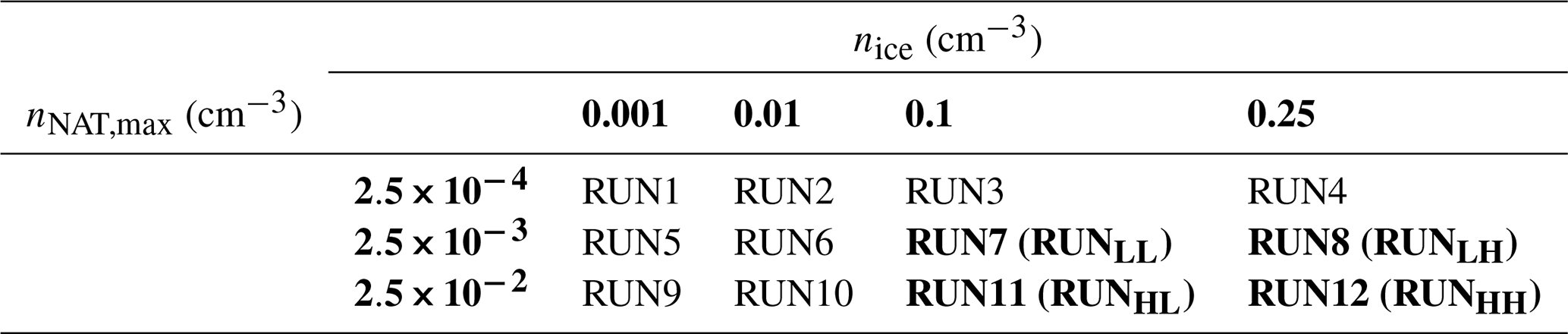
Twelve simulations were performed using the updated PSC parameterisation with varying values defined for n_NAT,max and n_ice to conduct a sensitivity analysis assessing the effect of the prescribed parameters on PSC formation. In the implementation of the same kinetic NAT parameterisation used here, Kirner et al. (2011) and Weimer (2019) use n_NAT,lim,b values of the order of 10⁻⁵ cm⁻³ resulting in a total maximum number density limit, $n_{\text{NAT,max}}={\sum }_b{n}_{\text{NAT,lim},b}$, of the order of 10⁻⁴ cm⁻³ based on measurements of Fahey et al. (2001). Here, we additionally investigate the effect of increasing the n_NAT,lim,b values to the order of 10⁻⁴ and 10⁻³ cm⁻³ to cover the range of number densities observed (Fahey et al., 2001; Biele et al., 2001) and used to constrain CALIOP observations (Pitts et al., 2018). The size bins and different orders of magnitudes used for the n_NAT,lim,b are summarized in Table 2 and result in values of n_NAT,max equal to $\mathrm{2.5}\times {\mathrm{10}}^{-\mathrm{2}}$, $\mathrm{2.5}\times {\mathrm{10}}^{-\mathrm{3}}$, and $\mathrm{2.5}\times {\mathrm{10}}^{-\mathrm{4}}$ cm⁻³ (for n_NAT,lim,b values of the order of 10⁻³, 10⁻⁴, and 10⁻⁵ cm⁻³, respectively). For ice PSCs, where observations are limited, n_ice was set to 0.001, 0.01, 0.1, and 0.25 cm⁻³, sampling across the wide range of values used in other models (Tritscher et al., 2019; Steiner et al., 2021; Weimer et al., 2021; Zhu et al., 2017), as well as the ice number densities considered by Pitts et al. (2018). A summary of the simulations is presented in Table 3. To avoid redundancy, we focus on analysing results from RUN7, RUN8, RUN11, and RUN12 as they best match the optical properties from CALIOP observations while illustrating sensitivity to n_NAT,max and n_ice. These simulations have been renamed based on whether n_NAT,max or n_ice is relatively high (H) or low (L) with respect to the four selected simulations. For example, RUN8 has $n_{\text{NAT,max}}=\mathrm{2.5}\times {\mathrm{10}}^{-\mathrm{3}}$ cm⁻³ which is relatively low and n_ice=0.25 cm⁻³ which is relatively high, so it has been renamed RUN_LH. A control run (CONTROL) using the original PSC parameterisation was also performed for comparison.

Table 3 Parameter settings for total maximum NAT number density limit (n_NAT,max) and ice number density (n_ice) in cm⁻³ for each of the sensitivity simulations. RUN7, RUN8, RUN11, and RUN12 are selected for analysis in this study and are highlighted in bold and renamed according to whether n_NAT,max or n_ice is relatively high (H) or low (L) with respect to the four chosen simulations.

Finally, the occurrence frequency and areal coverage of PSCs simulated by RUN12 (RUN_HH) and CONTROL are analysed. This requires defining SAD thresholds for NAT, ice, and STS to identify an occurrence of each PSC type at an individual grid-cell. SAD thresholds of 0.1 and 1.0 µm² cm⁻³ are used to identify ice and STS containing grid-cells, respectively. For NAT, the threshold is defined as the theoretical NAT SAD reached when particles grow to r_NAT>1.0 µm in the new parameterisation, corresponding to a particle size comparable to NAT PSCs in the CONTROL. This avoids counting grid-cells with very small NAT SADs and results in a NAT threshold of 0.015 µm² cm⁻³ for RUN_HH. Due to the known issues with the CALIOP SAD product mentioned above, observations are not included in this comparison.

3 Results

3.1 Comparison with optical properties from CALIOP

To assess the results from the simulations under conditions with temperatures consistently below the PSC formation thresholds, Fig. 1 compares the simulated optical properties from CONTROL and the four selected sensitivity runs (RUN_LL, RUN_LH, RUN_HL, and RUN_HH) with CALIOP observations over the Antarctic from 10–18 July 2008. Note that while the values of the counts of observations for CALIOP and grid-cells for the simulations in the 2D histograms cannot be directly compared due to their different spatial resolutions, their relative abundance can be compared qualitatively. During this period, CALIOP observations show distinct peaks in the NATmix and ice regions, with few points corresponding to the other three composition types (enhNAT, STS, and wave ice). In contrast, CONTROL shows a distinct peak in the enhNAT region with a tail in the NATmix and no points classifying as ice. The CONTROL also has a narrower R₅₃₂ range than CALIOP, resulting in fewer PSC types represented. (Note that since CONTROL includes no STS particles, the STS optical signal likely arises from NAT and ice with very low number densities.) The sensitivity runs generally capture the observed spread of the R₅₃₂ values better than CONTROL, which results in comparatively more points being classified as STS. The sensitivity simulations with higher n_ice (RUN_HH and RUN_LH) have optical properties extending into the ice region, however they don't cover the same range of optical properties in the ice region as the CALIOP observations. While CALIOP has a substantial number of observations with R₅₃₂ values ranging from 5 to 20, the maximum R₅₃₂ value achieved by the sensitivity simulations is around 6. Additionally, none of the sensitivity simulations have points with high enough R₅₃₂ values to be classified as wave ice. Instead, they exhibit a relative maxima in either the enhNAT or ice regions, depending on the choice of n_ice. The sensitivity simulations with larger n_NAT,max values (RUN_HL and RUN_HH) have more points in the NATmix region, whereas the lower n_NAT,max sensitivity simulations (RUN_LL and RUN_LH) have slightly more points in the STS region. Optical properties from all 12 sensitivity runs demonstrate a relatively strong dependence on n_NAT,max and n_ice, and are shown in Fig. S1 in the Supplement.

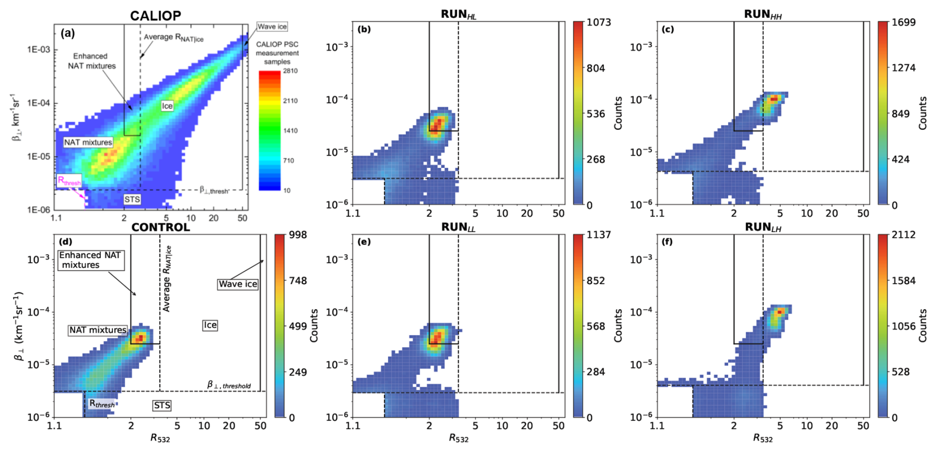
Figure 1 2D histogram of optical properties from CALIOP (a), RUN_HL (b), RUN_HH (c), CONTROL (d), RUN_LL (e), and RUN_LH (f) over the Antarctic for the period 10–18 July 2008, latitude range 65–75° S, and potential temperature range 475–525 K. The optical properties are plotted in the CALIOP v2 classification coordinate system of R₅₃₂ vs. β_⟂, with regions of enhanced NAT mixtures (enhNAT), liquid-NAT mixtures (NATmix), STS, ice, and wave ice indicated. The shading indicates the number of CALIOP observations (a), or the number of model grid points (b–f). Dashed lines indicate the mean β_⟂ and R₅₃₂ thresholds (including measurement uncertainty), as well as the mean R_NAT|ice boundary, calculated for CALIOP and each simulation separately. Solid lines indicate the boundaries separating wave ice and ice and enhNAT and NATmix. The regions labelled for CONTROL (d) are the same for all the sensitivity simulations (b, c, e, f).

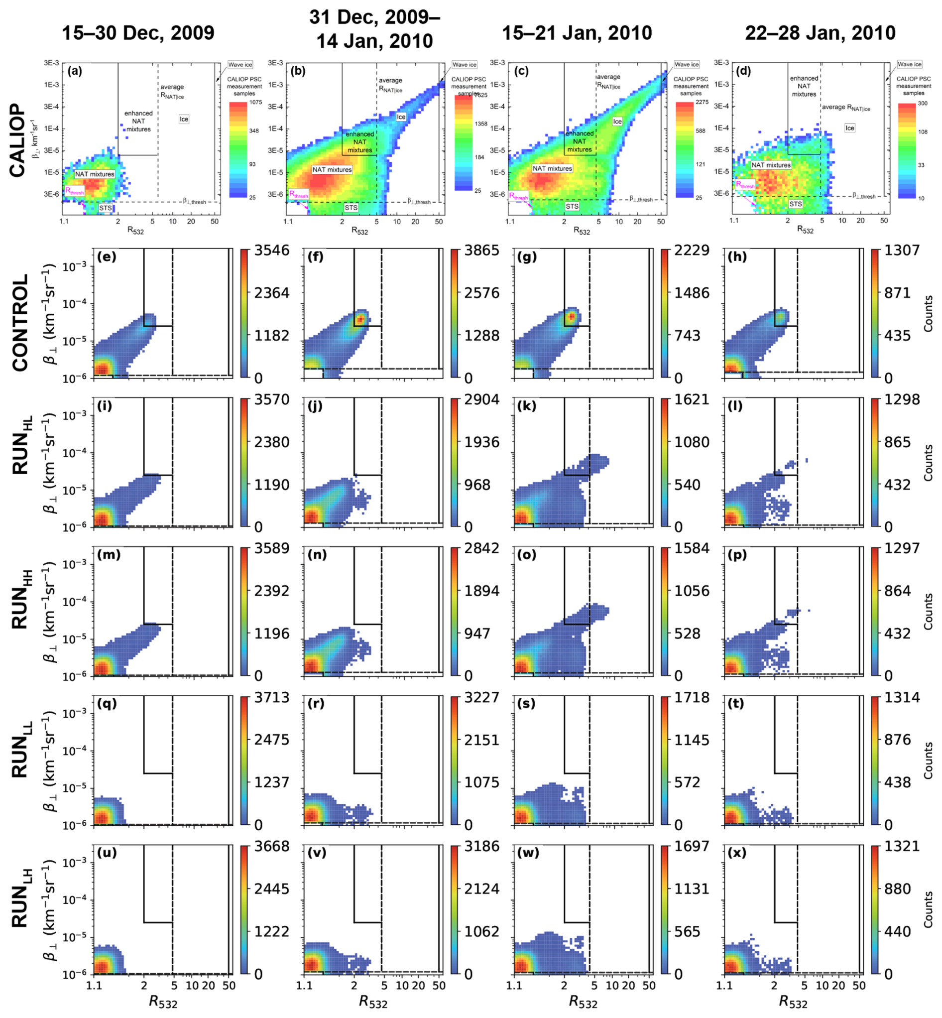
Figure 2 2D histogram of optical properties from CALIOP (a–d), CONTROL (e–h), RUN_HL (i–l), RUN_HH (m–p), RUN_LL (q–t), and RUN_LH (u–x) over the Arctic for the 2009/2010 winter season, latitude range 65–75° N, and height range 15–30 km. The results are separated into four distinct periods, comprising 15–30 December 2009 (first column), 31 December 2009–14 January 2010 (second column), 15–21 January 2010 (third column), and 22–28 January 2010 (fourth column). The results are plotted with the same classification algorithm, shading, boundaries, and regions as Fig. 1.

To further evaluate the new parameteristion, Fig. 2 compares simulated optical properties from CONTROL and the four selected sensitivity runs (RUN_LL, RUN_LH, RUN_HL, and RUN_HH) with CALIOP observations during the 2009/2010 Arctic winter, with the season separated into four distinct periods. Over the first period, from 15–30 December 2009, CALIOP is dominated by NATmix with no ice observed. Over the next two periods from 31 December 2009–14 January 2010 and 15–21 January 2010, CALIOP shows an increase in NATmix, as well as the occurrence of enhNAT and STS particles, and wave ice. In the final period from 22–28 January 2010, the vortex warmed above T_ice and widespread PSC observations from CALIOP declined appreciably. Most remaining PSCs are NATmix or STS, with only a few ice particles. In contrast, CONTROL shows PSCs initially dominated by NATmix in the period from 15–30 December 2009, then dominated by enhNAT for the remainder of the season with a tail extending into the NATmix, exhibiting little variation throughout the season aside from the number of points classified as PSCs, i.e., little resemblance to CALIOP and almost no response to the changing atmospheric conditions.

Unlike CONTROL, the higher n_NAT,max sensitivity runs (RUN_HH and RUN_HL) show broadly similar variations in PSC types over the Arctic winter, though not as pronounced as CALIOP observations (Fig. 2). During the first period (15–30 December 2009), RUN_HL and RUN_HH classify most PSCs as NATmix, in agreement with CALIOP. While during the second period (31 December 2009–14 January 2010), both these runs have a higher density of points in the NATmix region and extend into the STS region, again in agreement with CALIOP observations, but missing the points classifying as enhNAT and ice that are observed by CALIOP. However, during the third period (15–21 January 2010), both these runs spread into the ice and enhNAT region and further into the STS region, resulting in closer resemblance to CALIOP. Although, as with the Antarctic case, none of the points reach high enough values of R₅₃₂ to be classified as wave ice and the extent of the points in the ice region is limited compared to CALIOP. During the fourth period (22–28 January 2010), both these runs show a decrease in NATmix, enhNAT, and STS, again similar to CALIOP. In contrast, RUN_LL and RUN_LH produce fewer PSCs that fall in the optical property classification range compared to RUN_HL and RUN_HH. However, while RUN_LL and RUN_LH show a similar temporal evolution of maximum R₅₃₂ values over the season (i.e., an increase, followed by a slight decrease) that RUN_HH and RUN_HL (and CALIOP) also show, the equivalent evolution of maximum β_⟂ values is not as evident. This results in no points in the enhNAT region or ice region over the entire season in RUN_LL and RUN_LH. Note that the mean β_⟂ and R₅₃₂ thresholds (including measurement uncertainty) are determined by the boundaries defined in Eqs. (14) and (15) and therefore shift based on the measured and modelled values. In Fig. 2, the mean β_⟂ threshold line is lower across all periods and simulations compared to CALIOP, indicating the generally lower β_⟂ values in the distribution of model optical values compared to CALIOP.

Figures 1 and 2 show that increasing n_NAT,max (i.e., comparing RUN_LL and RUN_LH to RUN_HL and RUN_HH; see Table 3) shifts more points from the region below both the β_⟂ and R₅₃₂ thresholds into the regions classified as NATmix, enhNAT, and ice. In contrast, increasing n_ice (i.e., comparing RUN_LL and RUN_HL to RUN_LH and RUN_HH) results in more points being classified as enhNAT or ice. The sensitivity to ice number density is more pronounced for the Antarctic case (Fig. 1), whereas sensitivity to NAT number density is more pronounced for the Arctic case (Fig. 2).

3.2 Temporal evolution of modelled PSCs

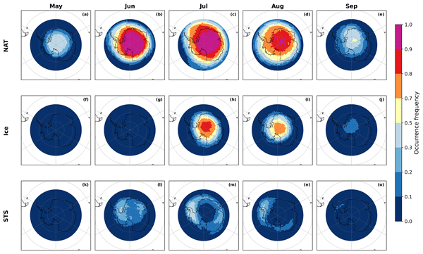
Figures 3 and 4 show the average PSC occurrence frequency over Antarctica at 20 km for NAT, ice, and STS for every month of the extended winter season over the entire 5-year simulation period of 2007–2011 for RUN_HH and CONTROL, respectively. RUN_HH was chosen as it shows the largest spread of optical properties compared with CALIOP (Fig. 1). Here, RUN_HH has high NAT occurrence frequency across Antarctica from June to August (values reaching 1), with lower frequencies in May and September (reaching 0.2). High occurrence frequency of ice (reaching 0.9) also occur during July and August, and are mainly concentrated over the centre of Antarctica. In contrast, STS only occurs from June to August in RUN_HH, particularly over Western Antarctica and the Antarctic Peninsula (i.e., near the edge of the stratospheric polar vortex), with much lower occurrence frequencies (reaching 0.2) – although this STS pattern is consistent with CALIOP observations (Pitts et al., 2018, Fig. 19 therein). CONTROL shows broadly similar patterns in both NAT and ice occurrence frequency as RUN_HH. The main differences are higher NAT frequency in May and September, reaching 0.7, and slightly lower ice frequencies in July and August. As CONTROL does not form STS, these results are not included in our comparison. The other sensitivity simulations show similar behaviour to RUN_HH (not shown). These results are further supported by the seasonal evolution of Antarctic PSC areal coverage for the extended 2008 winter season (see Fig. S2). Both CONTROL and RUN_HH show broadly similar areal coverage for NAT and ice PSCs, although there are slight differences in timing and vertical distribution. STS only forms in RUN_HH and starts having notable areal coverage later in the season and at a lower altitude than NAT. This results in both simulations showing broadly similar total PSC areal coverage over the entire winter season, although CONTROL has larger extent at higher altitude and RUN_HH at lower altitude.

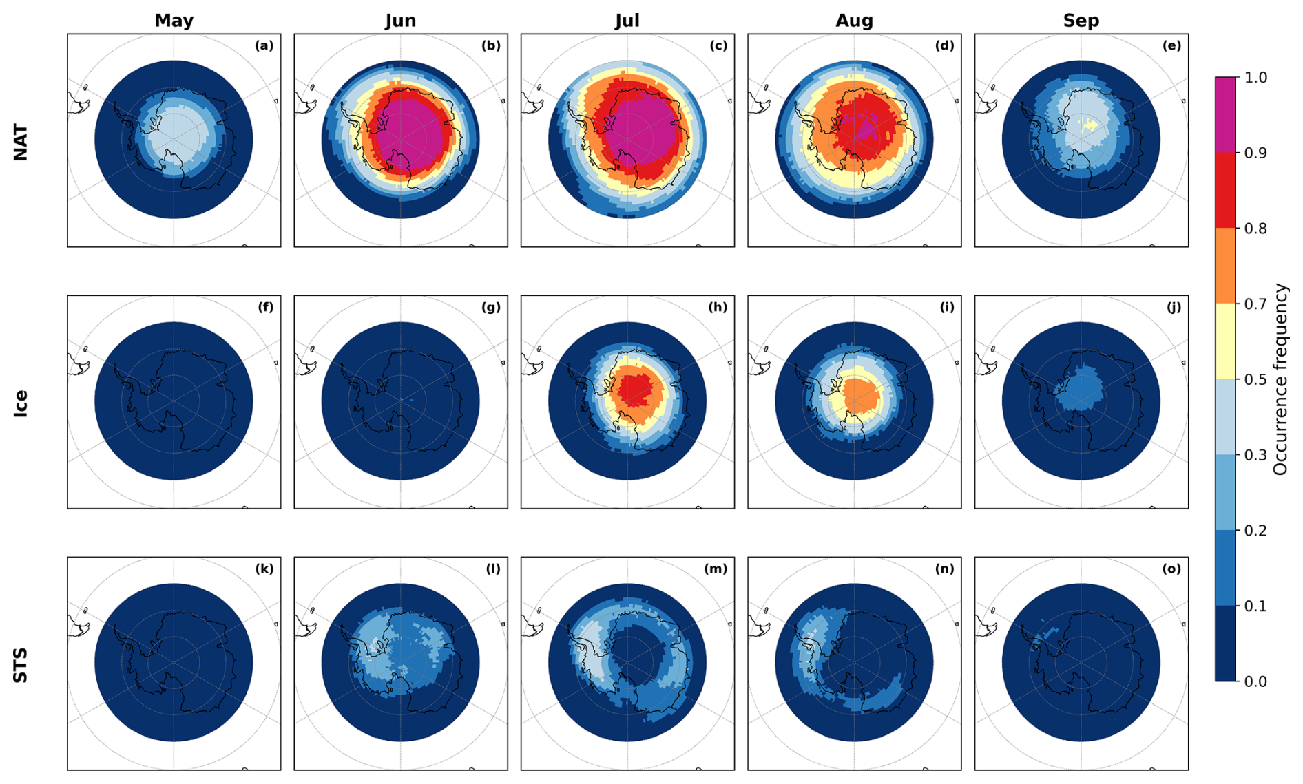
Figure 3 Monthly average PSC occurrence frequency over the Antarctic of NAT (a–e), ice (f–j) and STS (k–o) for May–September (left to right) over the 5-year period from 2007 to 2011 at an altitude of 20 km for RUN_HH. Occurrence frequency is defined as the number of days with PSC occurrence over the 5-year period for each month, divided by the total number of days over the 5-year period for each month.

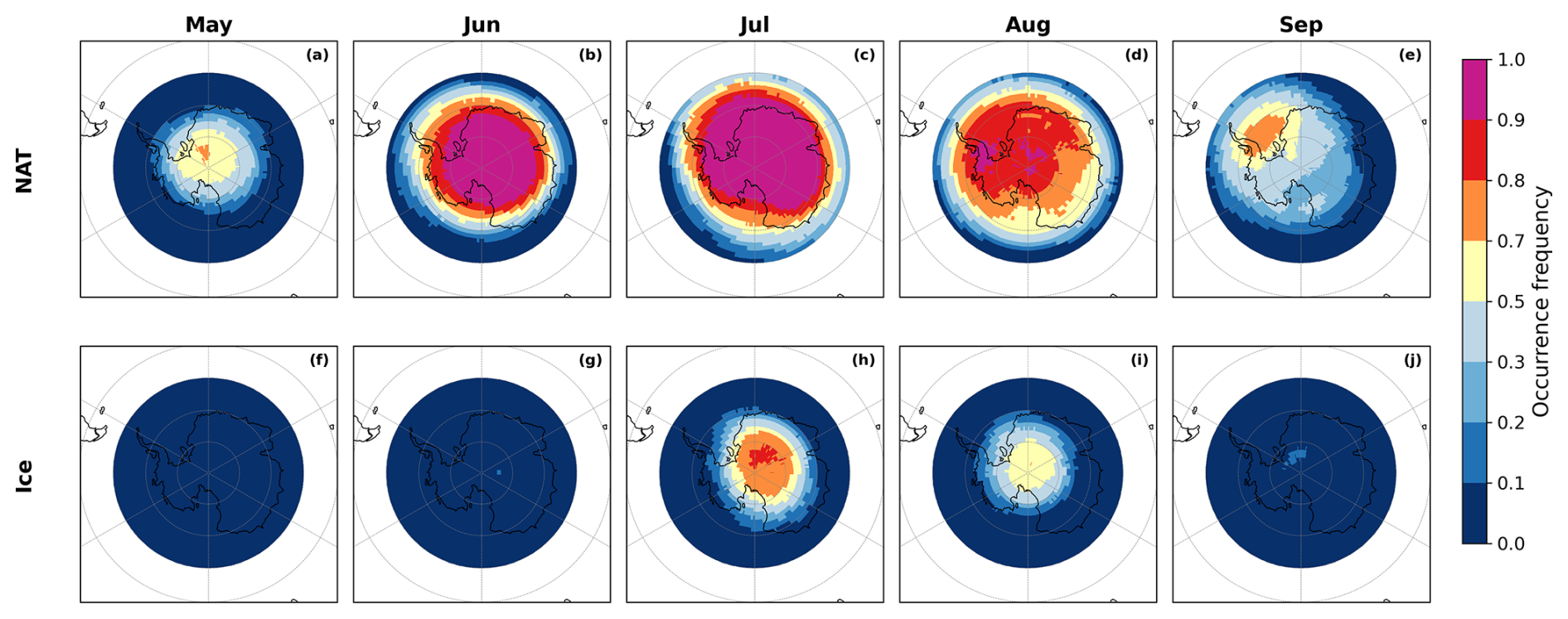
Figure 4 As in Fig. 3, but for CONTROL. Note that STS is not shown for CONTROL, as this is not simulated by the original PSC parameterisation.

To assess the seasonality and magnitude of SAD for the PSCs simulated by RUN_HH and CONTROL, Fig. 5 compares the temporal evolution of this quantity for NAT, ice, and liquid droplets (STS and sulphate aerosols) over the extended Antarctic 2008 winter. The smallest contribution to SAD for RUN_HH from the three PSC types is from NAT particles, which reach a maximum of around 0.36 µm² cm⁻³ in mid-June from around 16 to 22 km (Fig. 5a), despite NAT showing the largest spatial coverage (Fig. 3). In contrast, the opposite occurs for liquid droplets and ice in RUN_HH, which have much larger SAD (Fig. 5b and c) despite smaller spatial coverage (Fig. 3). Additionally, the peak in SAD for ice particles occurs slightly after that for NAT and at a slightly lower altitude range, while the occurrence of liquid droplets occurs at even lower altitude but with no distinct peak. Compared to RUN_HH, the SAD for NAT particles simulated by CONTROL is up to an order of magnitude higher (Fig. 5d). Differences in the distribution of SAD values for NAT particles simulated by CONTROL and RUN_HH across all grid-cells confirms this (Fig. S3), showing that CONTROL produces a narrow distribution of SAD for NAT particles concentrated at ∼ 1–10 µm² cm⁻³, while RUN_HH produces a broader distribution shifted to lower values of ∼ 0.01–1 µm² cm⁻³. The opposite is apparent for ice and liquid droplets (Fig. 5e and f), where CONTROL consistently has lower SAD than RUN_HH. Note that results for the other sensitivity simulations were broadly similar to RUN_HH (not shown), but with varying SAD magnitudes (see also Fig. S3).

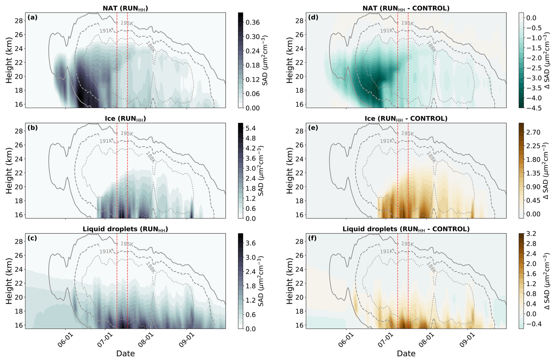
Figure 5 Time-height plot of zonal mean SAD (shading; µm² cm⁻³) for NAT (a), ice (b) and liquid droplets (STS and sulphate aerosols, (c) for RUN_HH over the Antarctic for the extended 2008 winter season (May to October), averaged across the latitude band 65–90° S. Also shown are the differences between RUN_HH and CONTROL for NAT (d), ice (e), and liquid droplets (f). Grey contour lines indicate T_NAT (solid), T_STS (dashed), and T_ice (dotted). The red dashed vertical lines indicate the period 10–18 July 2008 examined in Fig. 1. Note that the colour bar for all panels corresponds to different scales.

3.3 Comparison of HNO₃ and H₂O from MLS

To further assess the simulations, Fig. 6 compares gas-phase HNO₃ at 68 hPa from CONTROL and the four selected sensitivity runs (RUN_LL, RUN_LH, RUN_HL, and RUN_HH) with MLS measurements over the extended 2008 Antarctic winter. Over the latitude band 60–70° S (i.e., near the edge of the stratospheric polar vortex), MLS shows a gradual drop in gas-phase HNO₃ concentration from about 8 ppbv in June to 4 ppbv by August (Fig. 6a). By contrast, at 70–80° S (i.e., within the polar vortex), gas-phase HNO₃ concentration drops sharply in June from 8–10 to ∼ 2 ppbv and remains near this level until November (Fig. 6b), reflecting removal of HNO₃ from the gas-phase to form PSCs. While both the CONTROL and sensitivity runs have slight gas-phase HNO₃ depletion, they consistently underestimate gas-phase HNO₃ concentrations, especially in May before significant PSC formation. This likely reflects the known bias in low total reactive nitrogen (NO_y) in UKESM1.1 (Archibald et al., 2020). During the period of gas-phase HNO₃ depletion due to PSC formation, starting in mid-June, the underestimate of gas-phase HNO₃ concentration is most pronounced in CONTROL, with the sensitivity runs showing slightly higher gas-phase HNO₃ concentrations than CONTROL resulting in closer agreement to the MLS observations. A similar analysis at 100 hPa is presented in the Supplement (Fig. S4), showing consistent results with Fig. 6. Additionally, the same analysis is presented in the Supplement for the extended 2009/2010 Arctic winter at 68 hPa (Fig. S5). Here, there is not the same level of removal of gas-phase HNO₃, however the same low-bias in the models compared to MLS at the start of the Antarctic winter season is present throughout the entire Arctic winter season.

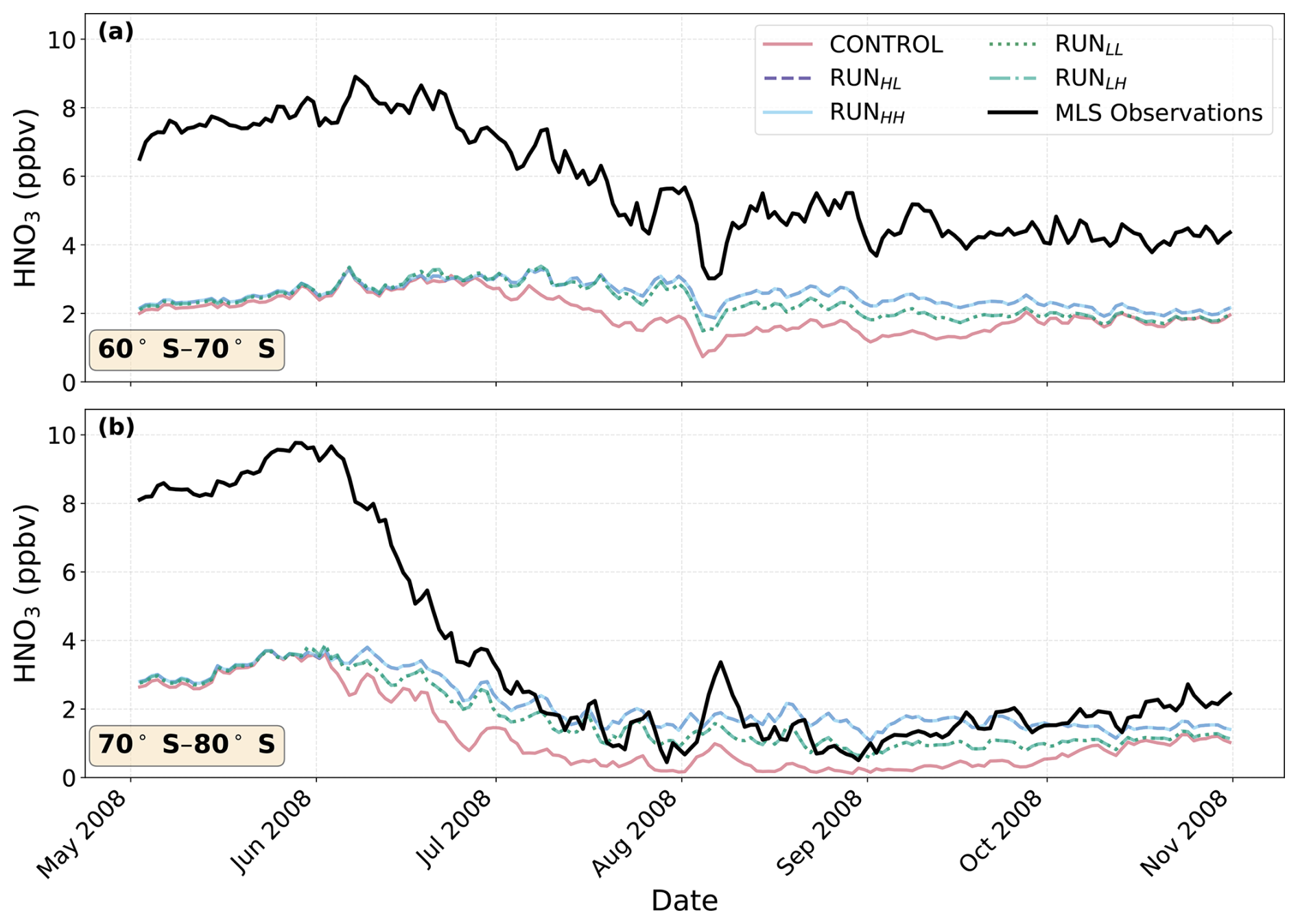
Figure 6 Zonal mean volume mixing ratio of gas-phase HNO₃ (ppbv) at 68 hPa for MLS (black line), CONTROL (pink line) and RUN_LL, RUN_LH, RUN_HL, and RUN_HH (purple, blue, green, and teal lines, respectively) over the Antarctic for the extended 2008 winter season (May to October), averaged across the latitude bands 60–70° S (a), and 70–80° S (b). Note that there is almost complete overlap of RUN_HH and RUN_HL, and RUN_LL and RUN_LH, resulting in only RUN_HH and RUN_LL being visible in the plot.

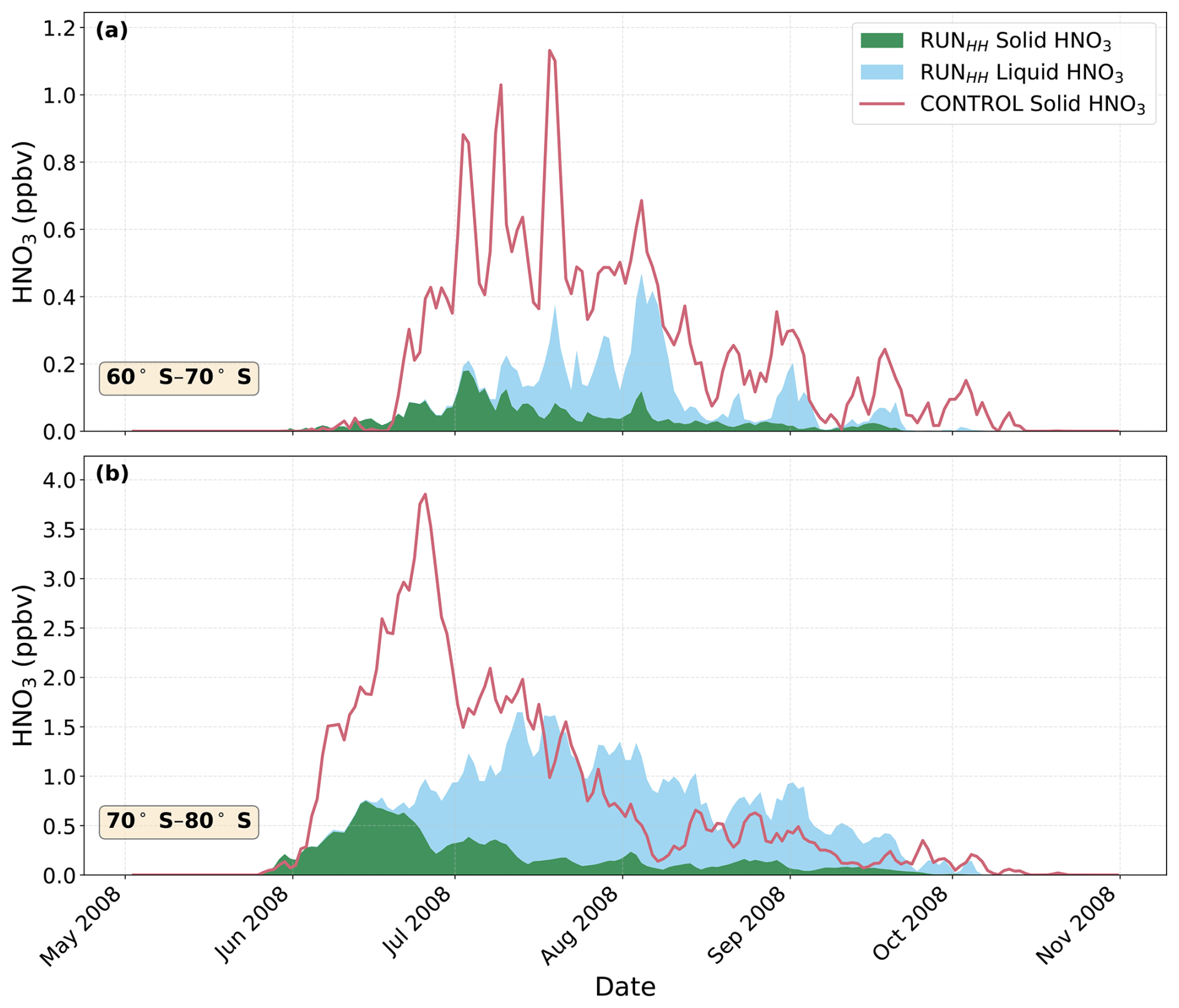
Figure 7 Zonal mean volume mixing ratio of solid- and liquid-phase HNO₃ (ppbv) at 68 hPa for CONTROL and RUN_HH over the Antarctic for the extended 2008 winter season (May to October), averaged across latitude bands 60–70° S (a), and 70–80° S (b). Solid-phase HNO₃ for CONTROL is shown with a pink line. The solid- and liquid-phase HNO₃ for RUN_HH are shown as a stacked area, with solid-phase in green and liquid-phase in blue. Note that liquid-phase HNO₃ is not shown for CONTROL, as this is not simulated by the original PSC parameterisation. Also, the panels have different scales.

The CONTROL and the sensitivity runs treat the removal of HNO₃ from the gas-phase differently: CONTROL converts all removed gas-phase HNO₃ to solid phase (NAT), whereas the sensitivity runs partition it between solid-phase and liquid-phase (STS). Figure 7 illustrates these differences for the extended 2008 Antarctic winter season by comparing the solid- and liquid-phase HNO₃ at 68 hPa from CONTROL and RUN_HH. The results show that RUN_HH starts partitioning HNO₃ from the gas-phase to solid-phase at roughly the same time as CONTROL (early June), but that the amounts of solid-phase HNO₃ simulated by CONTROL quickly surpasses RUN_HH. For example, over the latitude band 70–80° S the amount of solid-phase HNO₃ simulated by CONTROL peaks in mid-June before declining in late June–early July (Fig. 7b). Conversely, RUN_HH has a less-pronounced peak of solid-phase HNO₃ in mid-June over 70–80° S, followed by an increase in liquid-phase HNO₃ as STS forms. At 70–80° S, the combined solid- and liquid-phase HNO₃ simulated by RUN_HH becomes comparable to solid-phase HNO₃ simulated by CONTROL by July and exceeds CONTROL during August, September, and October. These shifts in the amounts of solid- and liquid-phase HNO₃ throughout the winter season are consistent with the changes in SAD (Fig. 5). A similar analysis at 100 hPa is shown in the Supplement (Fig. S6), which broadly agrees with Fig. 7.

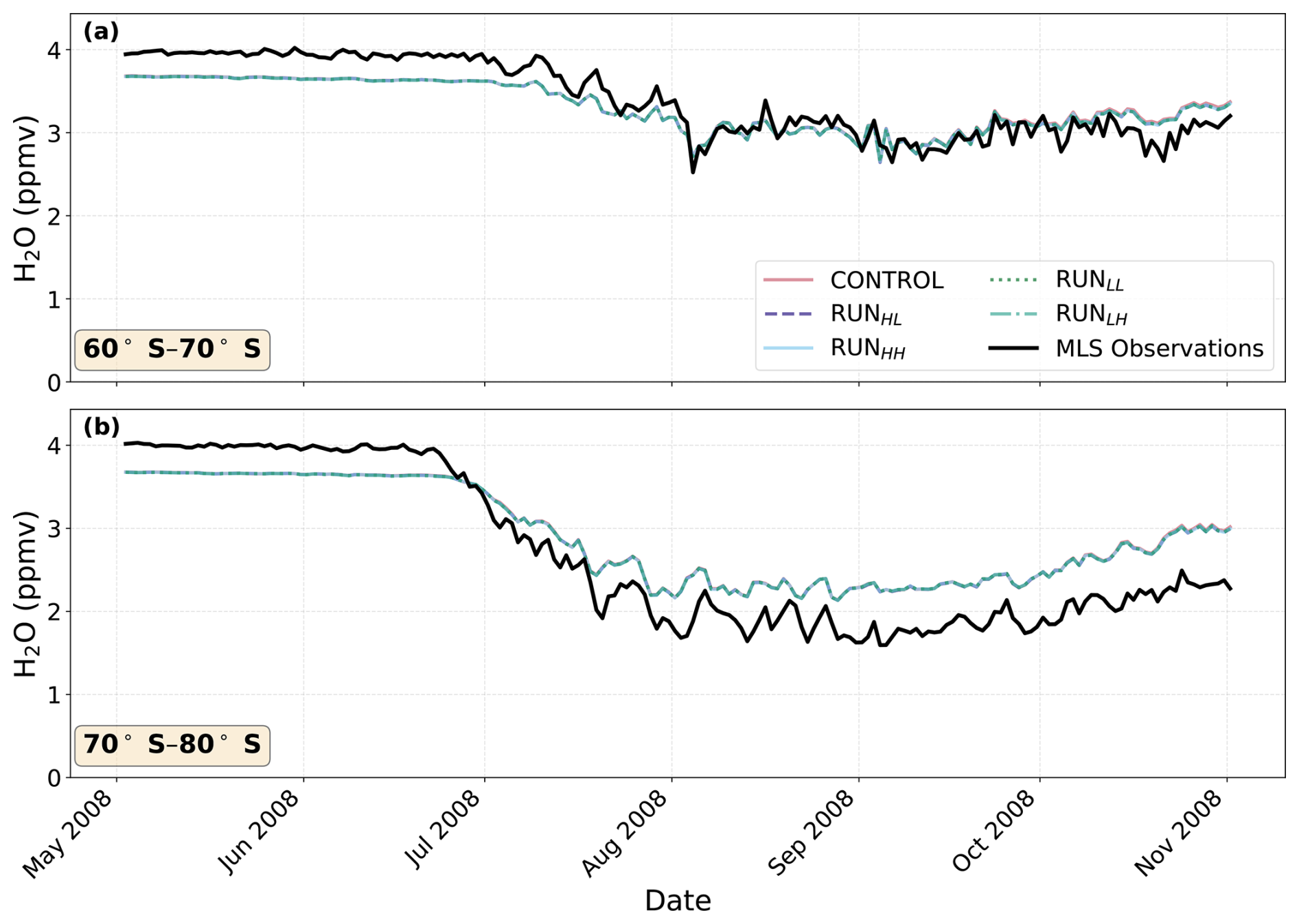
Figure 8 As Fig. 6, but for zonal mean gas-phase H₂O (ppmv) at 68 hPa. Note that there is complete overlap of all model runs (CONTROL and sensitivity simulations).

Stratospheric gas-phase H₂O is additionally analysed in Fig. 8 for the extended 2008 Antarctic winter. All model simulations produce the same gas-phase H₂O concentrations since ice is formed as a part of UKESM1.1's microphysics and is unchanged in the new PSC parameterisation. The new scheme only affects how ice mass mixing ratio is converted to SAD for heterogeneous chemistry. Furthermore, the amount of H₂O that condenses to form STS particles is negligible compared to the gas-phase H₂O concentrations. Compared to MLS, the model slightly underestimates gas-phase H₂O in May and June, but shows weaker dehydration from July to November. As a result, simulated gas-phase H₂O is comparable to MLS over 60–70° S (Fig. 8a) and higher than MLS over the 70–80° S (Fig. 8b). The same analysis is presented in the Supplement for the Arctic winter at 68 hPa (Fig. S7).

3.4 Comparison with ozone from MLS

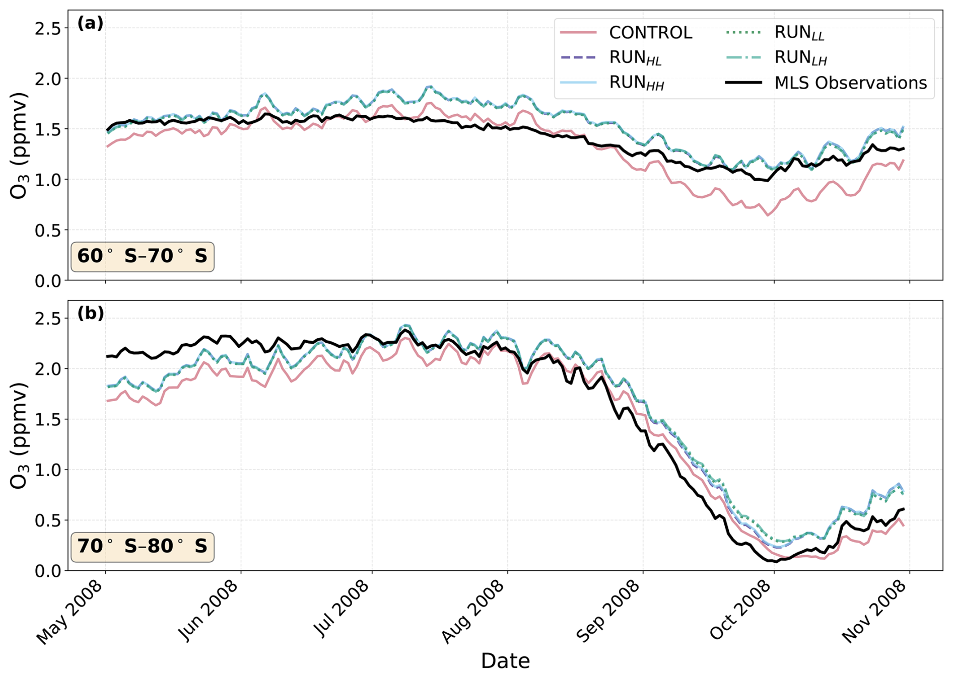
To assess how the simulations represent O₃, Fig. 9 compares the simulated O₃ at 68 hPa from CONTROL and the four selected sensitivity runs (RUN_LL, RUN_LH, RUN_HL, and RUN_HH) with MLS observations during the extended 2008 Antarctic winter, extending into early springtime to capture ozone depletion. The MLS data shows distinct O₃ loss starting around mid-August, reaching near-complete depletion over the latitude band 70–80° S by early October, when the Antarctic ozone hole tends to form. While both the CONTROL and sensitivity runs capture the timing of O₃ depletion at 60–70° S, CONTROL underestimates O₃ from September to October, whereas the sensitivity runs overestimate it from June to August (Fig. 9a). At 70–80° S, both the CONTROL and the sensitivity runs underestimate O₃ from May to June, but overestimate it from August to September, with the same bias persisting into October for the sensitivity runs (Fig. 9b). All four sensitivity runs show comparable O₃ concentrations. More generally, there is often little difference between the amount of O₃ simulated by CONTROL and the sensitivity runs, with the exception being over the latitude band 60–70° S (i.e., near the edge of the polar vortex) from September to October, where the sensitivity runs agree better with MLS. A similar analysis at 100 hPa is presented in the Supplement (Fig. S8), with these results in general agreement with Fig. 9.

Figure 9 As Fig. 6, but for zonal mean O₃ (ppmv) at 68 hPa. Note that there is almost complete overlap of RUN_HH and RUN_HL, and RUN_LL and RUN_LH, resulting in only RUN_HH and RUN_LL being visible in the plot.

4 Summary

This study attempts to improve the representation of PSCs in UKESM1.1 by replacing its current, simple scheme with a kinetic scheme for NAT formation and a thermodynamic scheme for STS formation. These improvements enhance UKESM1.1's ability to represent the diversity and seasonal evolution of PSCs. Comparisons with CALIOP observations for the 2008 Antarctic and 2009/2010 Arctic winters demonstrates that the new parameterisation scheme achieves closer agreement with CALIOP observations by increasing the number of points classifying as STS and ice and capturing seasonal variability in PSC types (Figs. 1 and 2). A sensitivity analysis using the new scheme reveals that n_NAT,max and n_ice directly influences the relative abundance of each PSC type (Figs. 1 and 2). Larger values of these parameters favour the formation of smaller particles with greater SAD (Fig. S3). Additionally, the influence of n_NAT,max is particularly strong in the Arctic, where warmer temperatures limit ice particle formation (Fig. 2). However, there is still a gap in the ability of the model to simulate high β_⟂ and high R₅₃₂ PSCs that are observed by CALIOP (Figs. 1 and 2).

The improvement in the diversity of PSCs simulated by the new scheme is further supported by an examination of the temporal evolution of PSCs over the Antarctic winter season (Figs. 3 and 4). While overall NAT and ice occurrence frequencies remain similar to the original scheme, the new scheme produces STS in regions where it was previously absent, especially near the vortex edge. Furthermore, analysis of SAD over the 2008 Antarctic winter shows that the new scheme produces a greater diversity of PSC types by slowing NAT growth and enabling the formation of STS droplets, resulting in STS contributing a greater proportion to the total PSC SAD than NAT, especially later in the season. (Fig. 5).

The updated scheme leads to modest improvements in gas-phase HNO₃ compared to MLS, particularly within the polar vortex, although all model simulations significantly underestimate HNO₃ (Fig. 6). The overall impact on stratospheric O₃ is small, but differences emerge near the polar vortex edge, where reduced O₃ loss from August to October brings the sensitivity simulations closer to MLS observations (Fig. 9). Conditions near the vortex edge are more variable, meaning changes in PSC formation, such as slowing the growth of NAT, may have a stronger influence on heterogeneous chemistry and ozone depletion. In contrast, changes within the vortex core are limited because ozone depletion is already close to saturation under persistently cold and isolated conditions (Kirner et al., 2015; Tritscher et al., 2021).

The severe underestimation of HNO₃ at the beginning of the PSC season, likely due to a known low-NOy bias in the UKESM1.1 stratosphere (Archibald et al., 2020), means that the improved comparison with observations of gas-phase HNO₃ from MLS using the new scheme does not necessarily imply an improvement in the ability of UKESM1.1 to accurately capture the full extent of HNO₃ depletion and denitrification. This is because UKESM1.1 begins the PSC/winter season with less HNO₃ than observed. This bias also affects NAT and STS formation since both depend on the partial pressure of HNO₃. The previous thermodynamic equilibrium approach may have partly compensated for this bias in terms of NAT formation by converting all excess gas-phase HNO₃ into NAT, whereas the new scheme slows NAT growth, making the effect of low HNO₃ on NAT formation more apparent. As a result, the reduction in NAT SAD in the new scheme reflects both slower NAT growth and enhanced STS formation, but is likely also amplified by the background HNO₃ bias. The origin of this bias requires further investigation.

The CONTROL and sensitivity runs produced less ice than observed by CALIOP and failed to form wave ice (Figs. 1 and 2). This likely arises from the prescribed ice number density, which constrains the ice particles to a narrow range of SAD (Fig. S3). This may limit the model's ability to reproduce the broader range of optical properties observed by CALIOP. Similar findings have been noted in other models (Weimer et al., 2021), suggesting that reproducing high-number-density ice particles requires a method that does not have a fixed prescribed ice number density. Additionally, adiabatic cooling from fine-scale mountain waves propagating into the stratosphere can cause rapid, localised cooling in the stratosphere that triggers the formation of ice PSCs, which in turn can seed NAT mother clouds downstream, resulting in high-number-density NAT and ice PSCs (Drdla et al., 2002; Voigt et al., 2003; Fueglistaler et al., 2003).

A parameterisation scheme that represented the cooling phase of these mountain-wave-induced temperature fluctuations was implemented in an earlier version of UKESM, and resulted in a considerable increase in the number of occasions that simulated stratospheric temperatures dropped below the threshold for ice PSCs (Orr et al., 2015, 2020). However, this scheme was not implemented in UKESM1.1, and so these effects are not represented in our simulations. This, combined with prescribing ice and NAT number densities, likely limits the formation of high-number-density PSCs in our simulations using the new PSC parameterisation scheme. To address this, implementing the mountain-wave-induced temperature fluctuation scheme and allowing n_ice and n_NAT,max to vary with cooling rate could improve the representation of PSC variability (Orr et al., 2015, 2020). Such development could further advance UKESM1.1's capability to simulate PSC formation and variability, contributing to more accurate projection of future changes in polar ozone and climate (Polvani et al., 2011; Previdi and Polvani, 2014).