Physics vs. AI in weather prediction: evaluating GraphCast, AIFS, and FuXi against an observation-corrected WRF model for flash floods

Data-driven artificial intelligence (AI) weather models are increasingly positioned as alternatives or complements to physics-based numerical weather prediction (NWP) systems, yet systematic model evaluation studies that compare both paradigms under controlled experimental conditions remain limited. Here we present a structured model evaluation framework applying standardised verification metrics to assess a regional WRF configuration against three publicly available AI models – GraphCast, AIFS Single 1.0, and FuXi – over three high-impact flood events in Luxembourg and the Greater Region (2016, 2018, and 2021), comprising around 90 simulated days per configuration and 92 119 matched forecast–observation pairs at a four-country network of 259 to 280 stations per event, each screened to be independent of the observations assimilated in that event (Fig. 1). The WRF model employs a three-dimensional variational (3D-VAR) data assimilation scheme ingesting GNSS Zenith Total Delay and conventional observations on a 6-hourly Rapid Update Cycle. All systems draw their initial and boundary information from the same ERA5 reanalysis, although the effective initial states are not identical: WRF is cycled and, in the assimilated configuration, corrected by observations, and ERA5 lateral boundary forcing of a limited-area model differs structurally from a global rollout. Categorical precipitation scores evaluated at thresholds from 1 to 20 mm (6 h)⁻¹ and continuous temperature metrics at surface stations serve as verification targets. Data assimilation raises WRF's categorical precipitation skill at the 1 mm threshold (Critical Success Index: 0.364 to 0.389, a difference not resolved by a block bootstrap over 24 h blocks) and brings the near-surface temperature bias close to zero, although this benefit does not extend to heavier rainfall: at 10 mm (6 h)⁻¹ the assimilated run scores below the unassimilated one. The degradation appears in all three events and is not ordered by the density of the assimilated observing network, so we report it without attributing a cause. At the 1 mm threshold AIFS achieves the highest detection rate (POD 0.835) and GraphCast the highest net categorical skill (CSI 0.424, against 0.415 for AIFS and 0.389 for the assimilated WRF), and AIFS and GraphCast reduce temperature RMSE by 19.0 % and 17.6 % relative to assimilated WRF at the subset of stations that also report temperature. This ordering reverses as the rainfall threshold increases: at 20 mm (6 h)⁻¹ WRF attains the highest skill (CSI 0.160), ahead of AIFS (0.141) and GraphCast (0.114), while FuXi produces no exceedances at all. A weather-radar comparison over 27 6 h periods shows the same reversal in space: AIFS holds the highest mean per-period Fractions Skill Score at 1 mm (6 h)⁻¹ at every neighbourhood width, but at 20 mm (6 h)⁻¹ both WRF configurations are ahead of all three AI models on that estimator, and a WRF configuration leads on the pooled aggregate as well. The per-event breakdown reveals no skill degradation for GraphCast on the 2021 event, which lies outside its training period – indeed its skill is highest there – demonstrating useful skill on this later event without identifying the cause of the event-to-event differences; the same test cannot be applied to AIFS, whose fine-tuning window encompasses all three events. These results provide a replicable model evaluation methodology for benchmarking emerging data-driven NWP systems against observation-corrected regional models.

1 Introduction

Accurate weather forecasting remains a critical challenge, particularly for predicting extreme events that can lead to catastrophic impacts such as the July 2021 European floods. For decades, conventional numerical weather prediction (NWP) models like the Weather Research and Forecasting (WRF) model have been the cornerstone of meteorological forecasting (Skamarock et al., 2019). These physics-based models rely on solving complex differential equations that govern atmospheric dynamics. However, they are computationally intensive and highly sensitive to initial conditions and parameterisation schemes (Prein et al., 2017; Nguyen et al., 2025; Mekawy et al., 2023; Fosser et al., 2024).

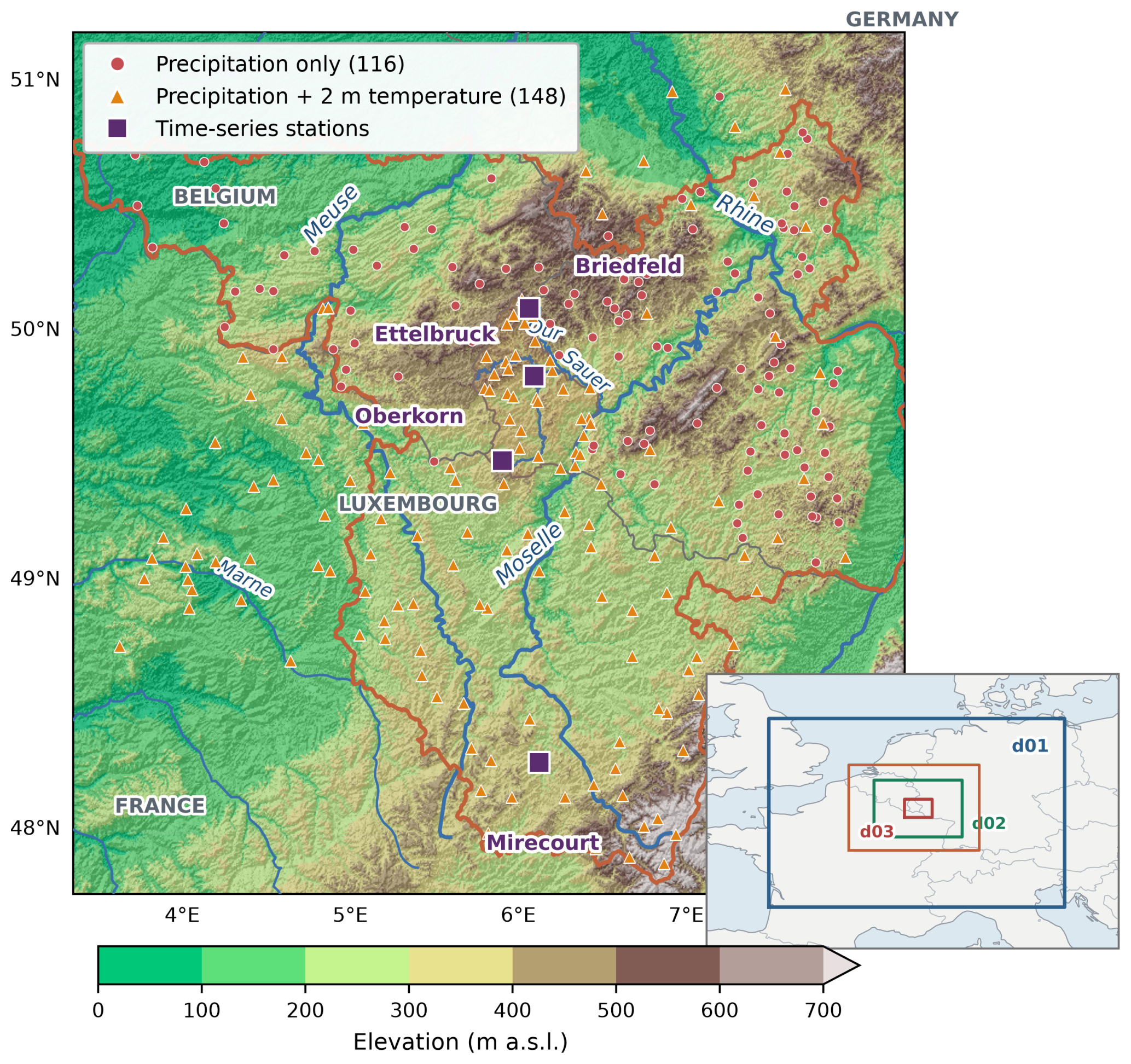
Figure 1 The study area and the independent verification network. The main panel zooms on Luxembourg and the Greater Region (orange outline) over SRTM-derived topography, shaded in 100 m elevation bands, with the principal rivers in blue. Stations are those used for verification (Sect. 5.3); the network shown is the one used for the 2021 event. Every station in the network reports precipitation; red circles mark the 116 that report precipitation only, orange triangles the 148 that report both precipitation and 2 m temperature ($\mathrm{116}+\mathrm{148}=\mathrm{264}$). All 148 are scored for temperature (Sect. 5.3). Purple squares mark the four gauges of the Fig. 13 time series (Briedfeld, Ettelbruck, Oberkorn, Mirecourt). The inset shows the WRF domains – d01 (blue, 12 km), d02 (green, 4 km) and d03 (red, 1.33 km), the last two used only for the resolution experiment of Sect. 6.5 – and the extent of the main panel over Western Europe. Station counts differ between events and between variables; they are given in Sect. 5.3 and Fig. 8. Topography is derived from the NASA Shuttle Radar Topography Mission 30 m global dataset (SRTMGL1, NASA JPL, 2013); national boundaries, coastlines and the ocean mask are from Natural Earth (https://www.naturalearthdata.com, last access: 9 October 2026, public domain). The Greater Region outline and the river network were produced by the authors.

Recently, artificial intelligence (AI) models have emerged as a disruptive technology in weather forecasting. Models such as GraphCast (Lam et al., 2023), Pangu-Weather (Bi et al., 2023), FourCastNet (Pathak et al., 2022), FuXi (Chen et al., 2023), the Artificial Intelligence Forecasting System (AIFS) (Lang et al., 2024), and Aurora (Bodnar et al., 2025), developed by leading research groups, leverage deep learning architectures and are trained on decades of historical reanalysis data. These data-driven models have demonstrated remarkable skill and computational efficiency (Kashinath et al., 2021; Wu and Xue, 2024; Bodnar et al., 2025; Weyn et al., 2021), often matching or exceeding the performance of conventional NWP models at global scales (Sham et al., 2025; Johny et al., 2026).

The comparative literature, however, points in two directions, and the tension between them motivates the present study. On one hand, Shirali et al. (2020) evaluated the WRF model against AI techniques for short-term rainfall, temperature, and flood forecasting in a regional case study and found that, while WRF provided physically consistent simulations of atmospheric processes, AI-based models achieved higher accuracy in predicting rainfall intensity and flood peaks. On the other, Zhang et al. (2026) showed that physics-based NWP models still outperform state-of-the-art AI systems for record-breaking extreme events, finding that AI models systematically underestimate the frequency and intensity of unprecedented extremes. These conclusions are not necessarily contradictory: they may simply describe different parts of the precipitation distribution, with data-driven models performing well for ordinary rainfall and losing their advantage as events become more extreme. Distinguishing between the two possibilities requires a comparison in which the same systems are verified over the same period, against the same observations, and across a range of rainfall intensities rather than at a single threshold. That is the design adopted here, applied to three flood events in a region where the catchment response leaves little margin for forecast error.

This study aims to conduct a comparative analysis between the physics-based WRF model (configured and tuned for Luxembourg and the Greater Region) and three AI-driven weather models: GraphCast, AIFS, and FuXi. By evaluating their performance across three high-impact flood events – the flash flood of 21–23 July 2016 in north-eastern Luxembourg, the Mullerthal flash flood of 31 May–2 June 2018, and the catastrophic 14–15 July 2021 European flood – we investigate the respective strengths and limitations of both approaches. Each event is simulated over a window of approximately one month (10 July–6 August 2016, 20 May–20 June 2018, and 20 June–20 July 2021). A single-domain (12 km) WRF setup with data assimilation, configured and tuned specifically for Luxembourg and the Greater Region, is used to provide a physics-based benchmark against the rapid inference capabilities of the AI models.

2 Study area

This study focuses on Luxembourg and the surrounding Greater Region (Fig. 1), a transboundary area whose contrasting terrain exerts a strong control on the hydrological response. Within Luxembourg itself, two physiographic units dominate the landscape. To the north lies the Oesling, the Luxembourg portion of the forested Ardennes massif, where mean elevations of roughly 450–500 m and steep, incised valleys favour rapid runoff. To the south, the Gutland comprises gentler, fertile lowlands with mean elevations near 200 m (Lucius, 1948; Muller, 1980; Waterlot et al., 1973). The region is drained by an interconnected river network: the Moselle, together with its tributaries the Sauer and the Our, forms the backbone of the system. Because many basins are small and steep, they respond quickly to convective rainfall, leaving only short lead times for warning.

The hazard was illustrated on 1 June 2018, when a near-stationary convective cell dropped extreme rainfall over the steep slopes of the Mullerthal and triggered severe local floods (Luxembourg Institute of Science and Technology, 2021). The July 2021 event was more catastrophic still, with specific discharges exceeding 1300 $\mathrm{l}{\mathrm{s}}^{-\mathrm{1}}{\mathrm{km}}^{-\mathrm{2}}$ in small basins such as the Bibeschbach (Luxembourg Institute of Science and Technology, 2021). Such episodes underline the need for forecasting systems able to resolve localised, high-intensity convection and the rapid runoff it generates.

3 Atmospheric modelling system

3.1 Weather Research and Forecasting model

The WRF model is a community mesoscale NWP system developed by the National Center for Atmospheric Research (NCAR) and partner institutions (Skamarock et al., 2019). The present study uses the Advanced Research WRF (ARW) core, configured as a single domain at 12 km horizontal grid spacing covering Luxembourg and the Greater Region (Fig. 1). The domain comprises 120×120 horizontal grid points with 33 terrain-following vertical levels and a model top at 50 hPa, integrated with a 60 s time step. All simulations were performed with WRF version 4.5. The physics suite is summarised in Table 1.

Thompson et al. (2008)(Mlawer et al., 1997)Dudhia (1989)(Jiménez et al., 2012)(Tewari et al., 2004)(Hong et al., 2006)(Grell and Freitas, 2014)

Table 1 WRF physics parameterisation options used in this study.

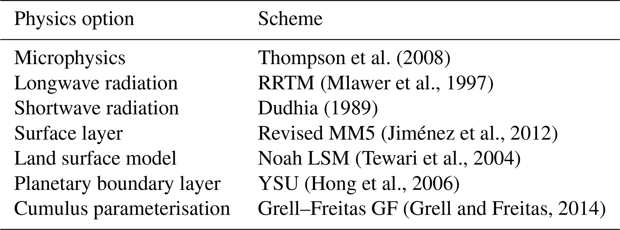
The domain was defined to cover the Greater Region because the synoptic systems responsible for these floods develop at that scale, while the hydrological focus, and hence the density of verification stations, is Luxembourg. The parameterisations in Table 1 follow published evaluations of WRF over neighbouring domains, supported by exploratory comparisons against station observations. The two choices that most directly govern convective rainfall at this grid spacing are corroborated by an independent systematic study: in an ensemble of 30 parameterisation combinations applied to eight extreme precipitation events over Germany, Stergiou et al. (2022) identified the Grell–Freitas cumulus and YSU boundary-layer schemes as the best-performing members of their respective groups, both of which are adopted here. Knist et al. (2018) likewise employed the Noah land surface model and YSU boundary layer in convection-permitting simulations over Central Europe. The Thompson microphysics scheme was retained for its double-moment treatment of ice and rain, which is well suited to the mixed-phase and orographically enhanced precipitation characteristic of the Ardennes–Eifel uplands. A comprehensive sensitivity analysis of the full physics suite lies beyond the scope of the present comparison and is left for future work. The background error covariance was not taken from a default dataset but generated specifically for this domain using the NMC method over a one-month period, as described in Sect. 3.2.

3.2 WRF data assimilation strategy

The 3D-VAR assimilation mode within the WRFDA system was employed. The primary objective of 3D-VAR is to minimise a quadratic cost function representing the discrepancy between the model analysis and both the background field and observations (Lorenc, 2003; Barker et al., 2004):

$$\begin{array}{}\text{(1)}& \begin{array}{rl}J\left(\mathit{x}\right)=& (\mathit{x}-{\mathit{x}}_{\mathrm{b}}{)}^T{\mathbf{\text{B}}}^{-\mathrm{1}}(\mathit{x}-{\mathit{x}}_{\mathrm{b}})\\ & +\left(H\right(x)-\mathit{y}{)}^T{\mathbf{\text{O}}}^{-\mathrm{1}}(H\left(\mathit{x}\right)-\mathit{y}),\end{array}\end{array}$$

where x_b is the background field, B is the background error covariance matrix, H is the observation operator, y represents the observations, and O is the observation error covariance matrix. The background error covariance was configured using the CV5 option with domain-specific statistics generated via the NMC method. The cost-function minimisation used two outer loops, and observations were accepted within a ± 1 h window centred on each analysis time.

3.3 NWP data and pre-processing

Initial and lateral boundary conditions were taken from the ERA5 reanalysis (Hersbach et al., 2020) at 0.25° resolution, sampled every 6 h across each 30 d window (Hersbach et al., 2023b, a). Conventional observations were drawn from the NCEP PREPBUFR archive and comprise SYNOP and METAR surface reports, TEMP radiosonde profiles, TAMDAR aircraft measurements (Daniels et al., 2006), and satellite atmospheric motion vectors (SATOB). In addition, GNSS ZTD observations were obtained from the Nevada Geodetic Laboratory (Blewitt et al., 2018). The composition of this observation set differs substantially between the three events, which proves important for interpreting the high-threshold results (Fig. 3 and Table 4).

Observations were assimilated on a 6-hourly cycle following the Rapid Update Cycle (RUC) strategy (Benjamin et al., 2004). The model is first cold-started from ERA5 to produce a spin-up; thereafter, each analysis updates the short-range first guess with the available observations, and the corrected state initialises the next cycle (Fig. 2).

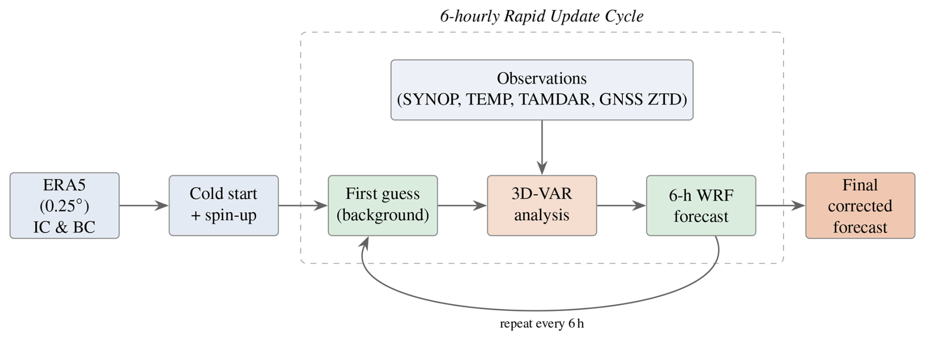
Figure 2 The WRF/WRFDA Rapid Update Cycle (RUC). The model is cold-started from ERA5 and spun up; thereafter, every 6 h the short-range forecast (first guess) is combined with conventional and GNSS ZTD observations in a 3D-VAR analysis that initialises the next 6 h forecast. After repeated cycling, the final observation-corrected forecast is launched.

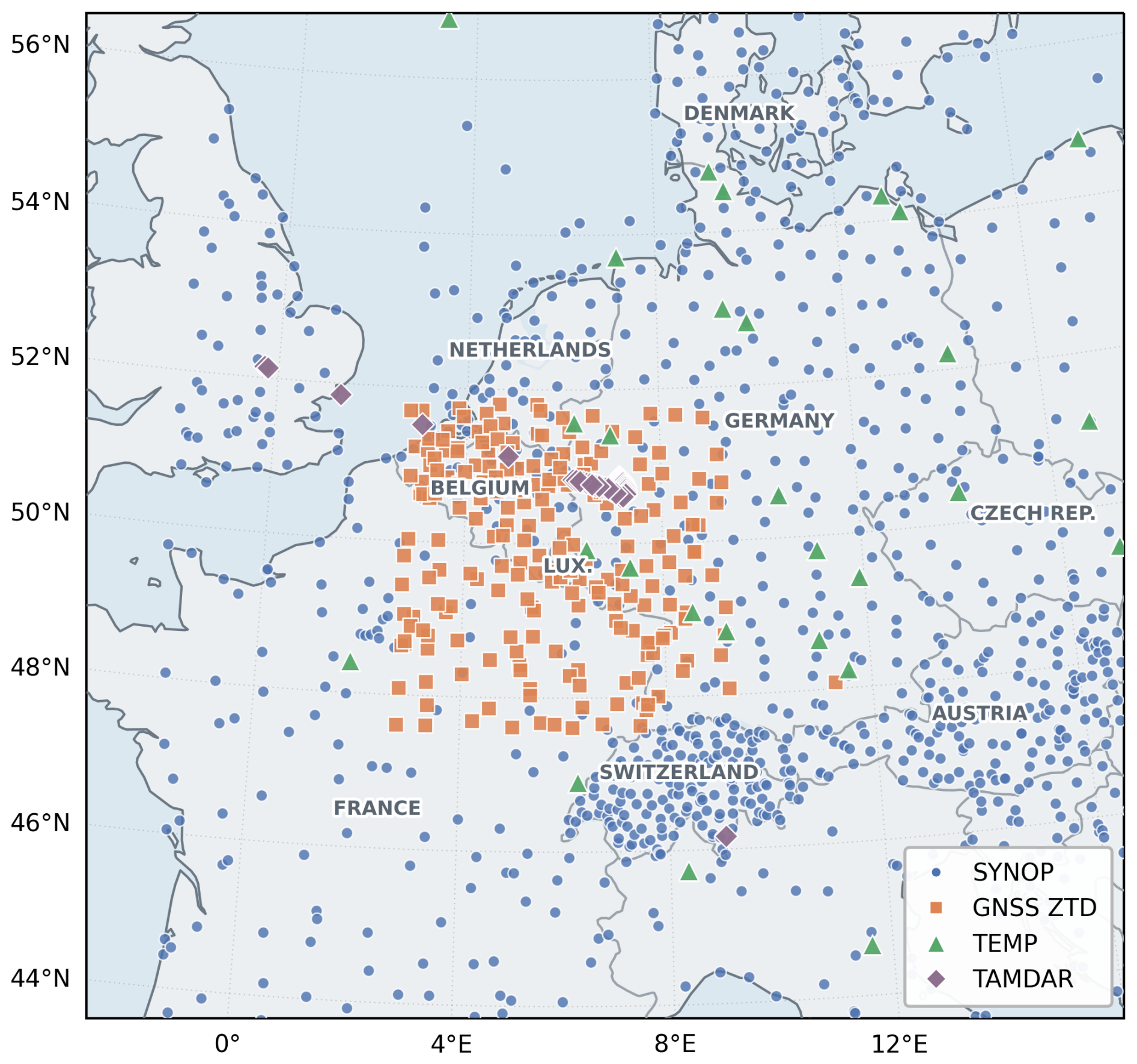
Figure 3 Spatial distribution of observations assimilated into the WRF 3D-VAR system: SYNOP surface stations (blue circles), GNSS ZTD sites (orange squares), TEMP radiosondes (green triangles), and TAMDAR aircraft reports (purple diamonds). The panel shows the 2021 event. The observing system differs considerably between the three events, so both the number and the distribution of the assimilated observations change from event to event: the 12 km independence screen of Sect. 5.3 is applied against 921, 904 and 1357 distinct assimilated surface positions in 2016, 2018 and 2021 respectively. Per-event counts by observation type are given in Table 4.

Verification observations were assembled from four national and regional archives: the Luxembourg AgriMeteo network (Administration des Services Techniques de l'Agriculture (ASTA), 2025), the German Weather Service, Météo-France and the Walloon SPW network. Station lists, per-event completeness and the screening applied to each are given in the accompanying data files. Hourly composite weather-radar rainfall accumulations for the July 2021 event were obtained from the RADFLOOD21 product of the Royal Meteorological Institute of Belgium (Goudenhoofdt et al., 2023) and aggregated to 6 h totals.

3.4 Post-processing

Meteorological variables were extracted from the WRF output using a custom Python workflow built on GDAL (GDAL/OGR contributors, 2023). Model values at station locations are taken from the nearest grid point, using a cKDTree query on the model grid (Virtanen et al., 2020); the same nearest-neighbour rule is applied to all four systems so that they are sampled identically (Table 3). No spatial averaging or weighting is applied.

4 AI-based weather forecasting models

This study evaluates three distinct data-driven weather forecasting models: GraphCast, AIFS, and FuXi. These models were selected because, at the time the experiments were configured, their publicly available implementations exposed a precipitation field that could be used directly, unlike the Pangu-Weather release and the Aurora version then available. Later Aurora releases do provide precipitation (Bodnar et al., 2025); adding them is left to future work rather than claimed as impossible here.

GraphCast, developed by Google DeepMind, utilises a multi-scale graph neural network (GNN) trained on ERA5 reanalysis data from 1979 to 2017. It generates global forecasts at a horizontal resolution of 0.25° with a native 6 h time step (Lam et al., 2023).

AIFS is the data-driven forecasting system developed by ECMWF (Lang et al., 2024). We use AIFS Single 1.0, the most recent AIFS release that can be initialised entirely from ERA5. The subsequent AIFS 2.0 release adds coupled ocean-wave inputs that we could not supply from ERA5 alone within the same input schema, which would have broken the consistency of initial conditions across the compared models; we did not attempt to establish the minimal set of fields that would make it runnable from reanalysis. AIFS Single 1.0 operates on an N320 (∼ 28 km) grid and was fine-tuned using operational IFS analyses from 2016–2022.

FuXi, developed by Fudan University and the Shanghai AI Lab, is a cascaded transformer-based forecasting system (Chen et al., 2023). Like GraphCast, it was trained on ERA5 and operates at 0.25° horizontal resolution with 6-hourly steps. The key characteristics of the three AI models are summarised in Table 2.

Table 2 Characteristics of the AI-based weather forecasting models evaluated in this study.

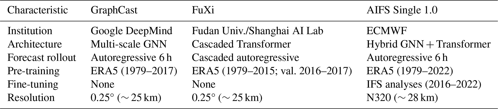
All three are trained on the same reanalysis, so that is not what separates them. What does separate them is what happens after pre-training: GraphCast and FuXi are used here exactly as pre-trained on ERA5, whereas AIFS Single 1.0 was subsequently rolled out on operational IFS analyses for 2016–2022 (Lang et al., 2024). That fine-tuning window covers all three of our case studies, which is why the AIFS results cannot be read as evidence of generalisation (Sect. 6.2.4). Where the text below groups two of the three models together it does so by result, not by provenance, except where it refers explicitly to the two models trained on reanalysis alone.

4.1 Model versions, inference settings and post-processing

Table 3 records the information required to reproduce the AI forecasts and their extraction to station locations.

Table 3 Model versions, inference settings and post-processing applied to the three AI systems. Precipitation is the native accumulated-precipitation field of each model over its 6 h step; all three report it in metres and it is converted to millimetres.

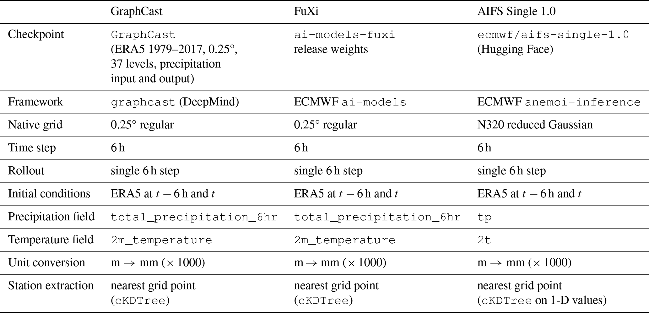
Exact checkpoint file names, sizes, checksums, Python environments and package versions are recorded in analysis/INFERENCE_MANIFEST.md in the archived repository (see Code and data availability). GraphCast was driven by a purpose-written runner on the public DeepMind checkpoint rather than through the ai-models command-line tool; FuXi used the short-range member short.onnx of the ai-models assets, so the cascade was not exercised; AIFS used the site module aifs-single-mse/1.0.2 with the 1.0 checkpoint pinned explicitly.

No bias correction, calibration or downscaling was applied to any AI output. ERA5 fields were retrieved from the ECMWF MARS archive (class=ea, expver=1, stream=oper) at 0.25° on the pressure levels each model requires. The same reanalysis is distributed through the Copernicus Climate Data Store; we name MARS because that is the retrieval actually executed, and the exact requests are archived with the code. For GraphCast and FuXi, which run on that same regular grid, the only pre-processing was selection of the variables and levels each model's input schema specifies, plus the 6 h accumulation of total_precipitation_6hr described below. AIFS runs on the N320 reduced Gaussian grid, and its inputs were retrieved from MARS directly on that grid (grid=N320), together with the constant fields it requires. No regridding of the AIFS input was performed, either by us or inside anemoi-inference. WRF fields were extracted to station locations with the same nearest-neighbour approach on the model grid, so that all four systems are sampled identically. Precipitation is the 6 h accumulation valid at the verification time in every case.

One input requirement differs between the three AI systems and deserves explicit statement, because it is a common source of error. The GraphCast checkpoint used here takes total_precipitation_6hr as a model input as well as an output, and it expects a genuine 6 h accumulation: the six consecutive hourly ERA5 totals ending at the initialisation time, summed. Supplying instead the single hourly total ending at that time – the value returned by the common “hourly, sampled at 00/06/12/18” retrieval – supplies the wrong accumulation period and degrades the forecast substantially. It is not in general six times too small: for steady rain the 6 h total is about six times the final hour, but rainfall is intermittent, so the ratio varies from zero to much more than six from cycle to cycle. The same file also carries toa_incident_solar_radiation, which must not be summed in the same way; only the precipitation field is accumulated. Neither of the other two systems has this requirement. FuXi accepts a precipitation channel but its released checkpoint does not use it: forecasts produced with the correct 6 h accumulation, with zeros, and with random values are identical to within machine precision. AIFS treats total precipitation purely as a diagnostic output and takes no precipitation input at all. All GraphCast results reported here use the correctly accumulated 6 h input.

5 Experimental design and verification

5.1 Case studies and simulation configuration

The two modelling systems were evaluated on three historic high-impact flood events over Luxembourg and the Greater Region: 2016, 2018, and 2021. Each event was simulated over a window of approximately one month (10 July–6 August 2016, 20 May–20 June 2018, and 20 June–20 July 2021), with forecasts initialised every 6 h, giving around 90 simulated days per configuration across the three events. The 2016 window is the shortest of the three, at 27 d, because the archived WRF output for that event ends on 6 August; the other two are full 30 d windows. Nominal 6-hourly sampling of a 30 d window gives about 120 valid times per event. Fewer are scored, because scores are computed only on the valid times common to all five products: 106, 122 and 117 6 h times enter the verification for 2016, 2018 and 2021, a total of 345 times or about 86 simulated days per configuration. The radar comparison of Sect. 6.4 uses 27 6 h periods and the resolution experiment of Sect. 6.5 22; neither is a subset of the station sample, since both are field-to-field comparisons. For WRF, two configurations were produced: a cold-start run without data assimilation (Before DA) and an observation-corrected run (After DA) using the 6-hourly RUC described in Sect. 3.3. WRF simulations were executed on 52 CPU cores of a high-performance computing cluster, distributed over dual-socket nodes with 28 Intel Xeon (Broadwell) cores each.

A 30 d window was chosen in preference to a window restricted to the flood days themselves. The first objective of the study is to establish whether 6-hourly assimilation of GNSS ZTD and conventional observations improves forecast skill, and a sample of two to four days does not contain enough independent precipitation events to separate that signal from sampling noise. The 30 d windows also include the pre-event synoptic evolution that conditions each flood, and they provide the model spin-up required by the Rapid Update Cycle. Scores restricted to the flood days alone are reported alongside the full-window scores in Sect. 6.2.6.

The three AI models were run on the same three events and 30 d windows. Forecasts were initialised from ERA5 analyses (at t−6 h and t) and advanced a single 6 h step to the verification time; each model was re-initialised from ERA5 every 6 h rather than rolled out freely. Inference was performed on a single NVIDIA A100 GPU with 40 GB of HBM2 memory. The 6 h cycling interval was chosen to align the products being compared. GraphCast, FuXi and AIFS all advance on a fixed 6 h native time step, which cannot be altered without retraining; that constrains the prediction interval, not necessarily the frequency at which forecasts could be launched, and off-synoptic initialisation is a separate question we have not tested. Cycling WRF more frequently would have given the physics-based system a shorter effective update interval than the products it is compared against. The sensitivity of the results to the cycling frequency is not examined here and we identify it as future work.

The computational contrast between the two approaches is large. On 52 CPU cores, one 6 h WRF cycle takes approximately 34 min without assimilation and 37 min with the 3D-VAR analysis included, so a complete 30 d window requires roughly 70 and 75 h of wall-clock time respectively. On a single NVIDIA A100 GPU, one 6 h AI forecast takes about 1.5 min, so the 120 initialisations of a 30 d window take about 30 min of inference. That is roughly 140 times faster than the physics-based chain for the same product, albeit after a training phase whose cost is borne once by the model developers. The timings are wall-clock for the forecast step alone and exclude ERA5 retrieval, checkpoint loading and output writing.

5.2 Scope of the three evaluations

Three distinct evaluations are reported, each covering the largest period for which the necessary observations exist. They are summarised here so that the domain of validity of each result is unambiguous.

The model intercomparison (Sect. 6.1–6.2.6) covers all three flood events over their full evaluation windows, verified against surface stations. This is the primary evaluation and provides the categorical and continuous scores.

The verification against weather radar (Sect. 6.3 and 6.4) is restricted to the July 2021 event. The RADFLOOD21 composite was produced specifically for that flood and is extensively documented (Goudenhoofdt et al., 2023); no equivalent open radar product covers the 2016 and 2018 events. It has two parts. Section 6.3 compares the fields visually at the three 6 h periods spanning the peak, 14 July 18:00 to 15 July 06:00 UTC. Section 6.4 scores them with the Fractions Skill Score over the 27 6 h periods from 11 July 06:00 to 17 July 18:00 UTC for which the radar total is complete and every system has a field.

The resolution experiment (Sect. 6.5) is restricted further, to the 22 6 h periods from 12 July 12:00 to 17 July 18:00 UTC, because the 4 and 1.33 km nests were not integrated before that time. It is therefore a targeted test of one question, whether horizontal resolution explains the behaviour seen at 12 km, and its results are not carried into the pooled statistics.

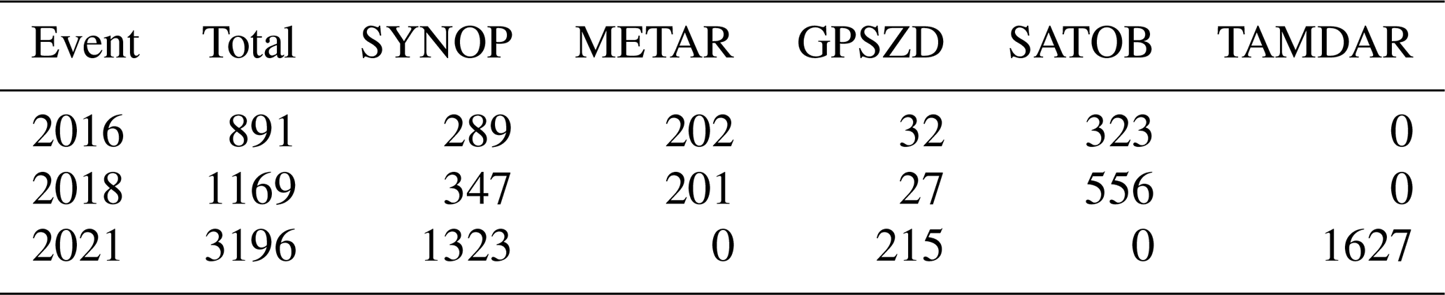
A point of uniformity should be stated explicitly, because the three events differ in the observations available for assimilation (Table 4). That heterogeneity affects the input to a single configuration, WRF (After DA). In every event all systems draw on the same ERA5 fields, are advanced on the same 6-hourly cycle, and are verified against the same station network with the same metrics and the same matching procedure. The verification is therefore uniform across the three events. The initial states themselves are not identical, and we do not claim they are: the AI models are re-initialised directly from ERA5 at each cycle, whereas the WRF first guess is a 6 h forecast from the previous cycle and, in the assimilated configuration, is corrected by observations. This study is best read as a comparison of ERA5-driven 6 h hindcast systems that includes an explicit WRF assimilation sensitivity, rather than as an isolation of physics from data-driven formulation under identical initial states. We regard this variation as a property of the observing system rather than of the experimental design, since aircraft reporting depends on commercial air traffic and GNSS coverage depends on which regional archives extend back to a given event.

Table 4 Observations assimilated per 6-hourly analysis cycle, averaged over every analysis cycle inside each event's verification window (109, 125 and 121 cycles). GPSZD is GNSS zenith total delay, SATOB satellite atmospheric motion vectors, and TAMDAR aircraft observations. The listed platforms do not sum to the total: the balance is 45, 38 and 31 reports per cycle, made up of TEMP radiosondes (10, 10 and 31), SHIP (15, 11 and 0) and BUOY (19, 16 and 0) reports, which are assimilated but not broken out here. The 2021 cycles contain no METAR or SATOB reports; that is the composition of the archive for that event.

5.3 Verification network and its independence

Verification uses surface stations that are independent of the observations assimilated into WRF. Two criteria were applied. First, any station lying within 12 km of a surface observation assimilated in that event's own analyses was excluded; the assimilated positions were taken from the observation files actually ingested by the Rapid Update Cycle rather than assumed, and the screen was applied separately for each event. Second, stations whose records cannot support a 6 h accumulation, several of which report only 12 or 24 h totals, were excluded, retaining only those supplying at least 95 % of the 6-hourly windows. The retained networks comprise 259, 280 and 264 stations for precipitation in 2016, 2018 and 2021. Of these, 119, 134 and 148 stations also carry a 2 m temperature channel and pass the same two criteria, and the temperature scores reported below are computed on those; the smallest station-to-observation separation anywhere is 12.04 km. The counts differ between events because the available station networks themselves differ – gauges are commissioned and decommissioned, records begin and end, and the assimilated observing system was denser in 2021 – not because a different rule was applied. For the 2021 event the retained network comprises 105 German, 92 French, 34 Luxembourgish and 33 Belgian stations occupying 234 distinct 12 km model grid cells. All 264 report precipitation; 148 of them report 2 m temperature as well, leaving 116 that report precipitation only (Fig. 1). The two variables use different networks because not every station reports both: the Belgian SPW gauges are precipitation-only, only a subset of the German stations carries an hourly temperature record, and fewer still report it without long gaps.

It should be emphasised that precipitation, the primary verification variable, is not assimilated by any observation type in this configuration. The WRFDA observation files carry only pressure, wind speed and direction, height, temperature, dew point and humidity, together with sea-level pressure and precipitable water; radar reflectivity and rain-rate assimilation are disabled. No precipitation observation therefore enters the regional analysis, and the station-selection criteria extend the same separation to the 2 m temperature verification. Two limits on that statement should be kept in view. The assimilated temperature, humidity and wind observations can inform the model's rainfall indirectly, so the verification is independent of direct reuse rather than statistically independent of the analysis. And ERA5, which supplies the initial and boundary conditions for every system here, has itself assimilated many of the same observing networks.

The retained network spans four countries and samples the model domain rather than concentrating on the hydrological area of interest. For the 2021 event it comprises 105 German, 92 French, 34 Luxembourgish and 33 Belgian stations occupying 234 distinct model grid cells, and the 2016 and 2018 networks are similarly distributed. Two features are worth noting. The Luxembourg AgriMeteo gauges provide continuous 6-hourly records at high spatial density over the small, fast-responding catchments described in Sect. 2, and because they are agro-meteorological stations that do not report on the Global Telecommunication System they cannot enter an operational analysis: they are independent by construction rather than by selection. The German, French and Belgian stations, by contrast, sample the wider domain over which the responsible synoptic systems develop. The scores reported here therefore describe domain-scale performance and are not dominated by conditions in a single catchment.

5.4 Verification metrics

Because precipitation is intermittent and highly skewed, categorical scores derived from a 2 × 2 contingency table of forecast/observed rainfall occurrence at or above a threshold are used, with hits a, false alarms b, misses c, correct negatives d, and total $n=a+b+c+d$. The comparison is inclusive, ≥ rather than >. This is worth stating because 692 of the 92 119 observations in each model's sample are reported at exactly 1.0 mm, and would change category under the strict inequality:

$$\begin{array}{}\text{(2)}& {\displaystyle }\mathrm{POD}={\displaystyle \frac{a}{a+c}},\text{(3)}& {\displaystyle }\mathrm{FAR}={\displaystyle \frac{b}{a+b}},\text{(4)}& {\displaystyle }\mathrm{CSI}={\displaystyle \frac{a}{a+b+c}},\text{(5)}& {\displaystyle }\mathrm{ETS}={\displaystyle \frac{a-a_r}{a+b+c-a_r}},a_r={\displaystyle \frac{(a+b)(a+c)}{n}},\end{array}$$

where POD is the probability of detection, FAR the false-alarm ratio, CSI the critical success index, and ETS the equitable threat score. Scores are reported at a 1.0 mm (6 h)⁻¹ threshold throughout, and additionally at 5, 10 and 20 mm (6 h)⁻¹ in Sect. 6.2.5 to assess whether the conclusions depend on the rainfall rate considered. Near-surface temperature and precipitation amount were verified with continuous statistics over N forecast–observation pairs (F_i,O_i):

$$\begin{array}{}\text{(6)}& {\displaystyle }\mathrm{Bias}={\displaystyle \frac{\mathrm{1}}{N}}\sum _{i=\mathrm{1}}^N(F_i-O_i),\text{(7)}& {\displaystyle }\mathrm{MAE}={\displaystyle \frac{\mathrm{1}}{N}}\sum _{i=\mathrm{1}}^N\left|F_i-O_i\right|,\text{(8)}& {\displaystyle }\mathrm{RMSE}=\sqrt{{\displaystyle \frac{\mathrm{1}}{N}}\sum _{i=\mathrm{1}}^N(F_i-O_i{)}^{\mathrm{2}}},\text{(9)}& {\displaystyle }r={\displaystyle \frac{{\sum }_i(F_i-\stackrel{\mathrm{‾}}{F})(O_i-\stackrel{\mathrm{‾}}{O})}{\sqrt{{\sum }_i(F_i-\stackrel{\mathrm{‾}}{F}{)}^{\mathrm{2}}{\sum }_i(O_i-\stackrel{\mathrm{‾}}{O}{)}^{\mathrm{2}}}}}.\end{array}$$

For POD, CSI, ETS, and r, higher is better; for FAR, MAE, and RMSE, lower is better; the bias is best near zero. Bias, MAE and RMSE are used for the station verification of 2 m temperature; r is used only for the field-to-field comparison against radar (Sects. 6.3–6.5), where F_i and O_i are the model and radar values at the points of the common mesh rather than at stations.

6 Results and discussion

The results are presented in three stages. We first quantify the effect of data assimilation (Sect. 6.1), then benchmark WRF (After DA) against the three AI models (Sect. 6.2), and finally evaluate all systems against weather radar for the July 2021 flood (Sect. 6.3).

6.1 Impact of data assimilation on WRF forecasts

6.1.1 Precipitation

At the 1 mm (6 h)⁻¹ threshold used here, assimilation improves the detection-based precipitation scores. POD rises from 0.527 to 0.611 (+16.0 %), CSI from 0.364 to 0.389 (+6.7 %) and ETS from 0.288 to 0.306 (+6.1 %), at the cost of a slightly higher false-alarm ratio (0.458 to 0.483). The mean precipitation bias moves toward zero ($-\mathrm{0.220}\to -\mathrm{0.094}$ mm), consistent with the hypothesis that assimilated moisture information, GNSS ZTD among it, partially relieves the model's tendency to under-forecast totals. We have not isolated the contribution of any single observation type, which would require observation-denial experiments. This improvement does not carry over to heavier rainfall: Sect. 6.2.5 shows that at 5 and 10 mm (6 h)⁻¹ the assimilated run scores lower than the cold-start run, and that at 20 mm (6 h)⁻¹ the two are indistinguishable.

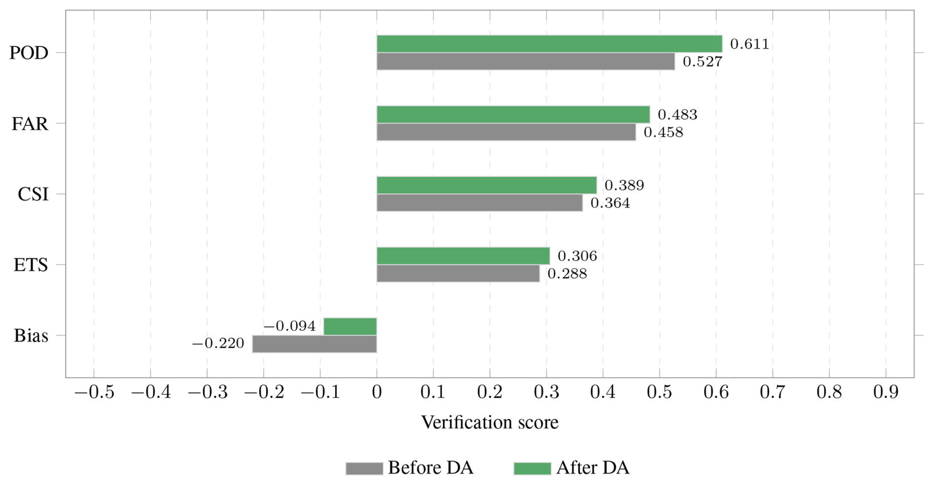
Figure 4 WRF precipitation verification before and after data assimilation, aggregated over the 2016, 2018, and 2021 events (90 simulation days). Higher POD, CSI, and ETS and lower FAR indicate better skill; the bias is the mean precipitation bias (best near zero).

6.1.2 Temperature

Near-surface temperature is largely insensitive to assimilation. RMSE and MAE shift only by a small amount in the wrong direction (1.880→1.916 and 1.439→1.479 °C), although the mean bias is brought closer to zero ($-\mathrm{0.203}\to -\mathrm{0.036}\mathit{°}$C). The paired bootstrap of Sect. 6.2.3 separates the two: the RMSE change is +0.036 °C (−0.008 to +0.083), an interval containing zero, whereas the bias improvement of +0.167 °C (+0.115 to +0.222) is resolved. One possible reading is that the assimilated network is weighted towards moisture-sensitive observations, so that 6-hourly cycling reshapes the humidity and mass fields more than the surface temperature; the observation counts in Table 4 are consistent with that but do not establish which observations dominate the analysis increment.

6.2 WRF and AI models compared

6.2.1 Precipitation

The comparison reveals clear distinctions among the models. GraphCast and AIFS both detect rain events far better than the regional model: AIFS reaches the highest detection rate (POD 0.835) and GraphCast follows closely (0.782), against 0.611 for the assimilated WRF. GraphCast attains the highest net categorical skill (CSI 0.424, ETS 0.330), marginally above AIFS (0.415, 0.315) and clearly above WRF (0.389, 0.306). The mean precipitation biases are small in all four systems: AIFS is marginally wet (+0.166 mm) and GraphCast almost unbiased (+0.043 mm), whereas WRF (−0.094 mm) and FuXi (−0.288 mm) are marginally dry, so none of the systems misrepresents the 6-hourly rainfall climatology of the verification period to a meaningful degree. FuXi consistently underperforms on both categorical metrics and bias. The assimilated WRF maintains a lower false-alarm ratio (0.483) than any of the AI systems, although the unassimilated run is lower still (0.458). As Sect. 6.2.5 shows, however, this ordering is specific to the 1 mm threshold and does not carry over to the heavier rainfall rates that matter for flash-flood warning.

6.2.2 Temperature

For near-surface temperature, AIFS and GraphCast show unambiguous advantages over WRF. AIFS attains the lowest RMSE (1.552 °C) and MAE (1.173 °C), with GraphCast close behind (1.580, 1.194 °C); both reduce RMSE substantially relative to the assimilated WRF (1.916 °C), by 19.0 % for AIFS and 17.6 % for GraphCast. Pooled RMSE is the square root of the mean squared error over all 45 925 matched pairs, not an average of the per-event values. AIFS is also the least biased system (+0.015 °C), ahead of the assimilated WRF (−0.036 °C) and GraphCast (+0.171 °C). FuXi underperforms significantly, with the highest errors and a pronounced warm bias (+0.609 °C).

6.2.3 Statistical significance of the differences

Because several of the differences in Figs. 6 and 7 are small, their sampling uncertainty is quantified by a bootstrap. Two features of the sample make the obvious choice inappropriate. Neighbouring stations share the same weather and sometimes the same model grid cell, and successive 6 h cycles belong to the same weather episodes, so the 92 119 matched pairs are far from 92 119 independent realisations; and a difference between two models is a paired quantity, which comparing two separately computed intervals does not test.

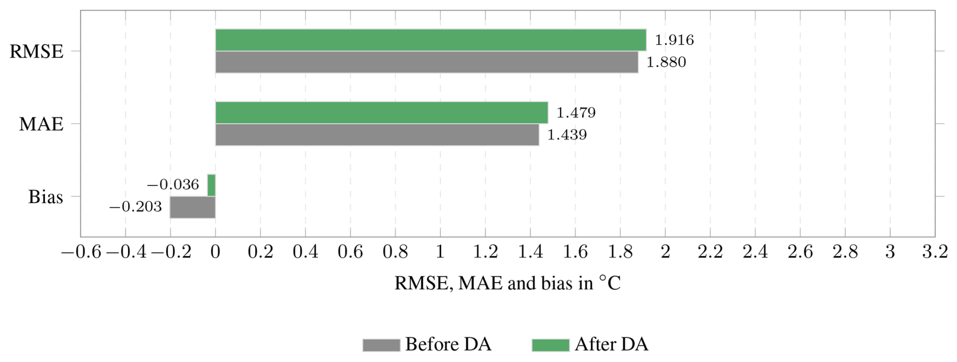
Figure 5 WRF 2 m temperature verification before and after data assimilation, aggregated over the 2016, 2018, and 2021 events. Lower RMSE and MAE are better, and the bias is best near zero.

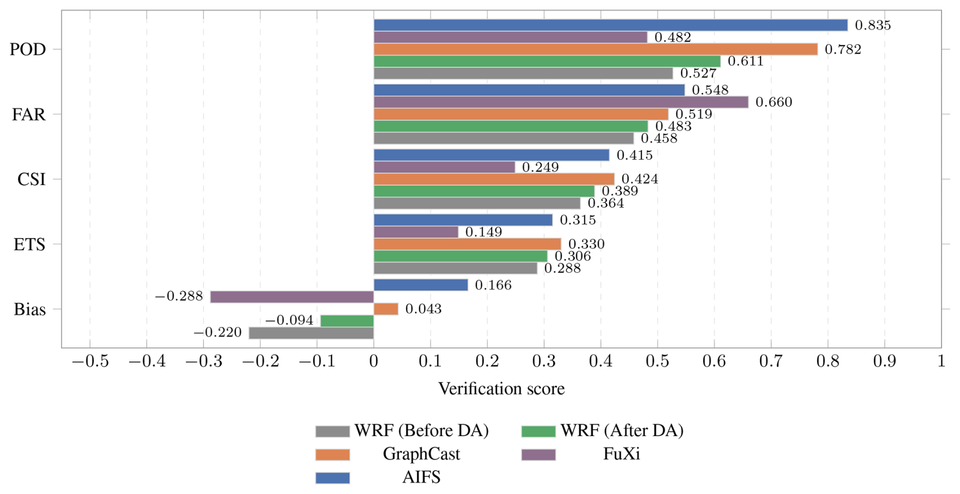
Figure 6 Precipitation verification of WRF versus the AI models over the common observation forecast pairs of the 2016, 2018, and 2021 events. Higher POD, CSI, and ETS and lower FAR indicate better skill; the bias is the mean precipitation bias (best near zero). All five products are scored on the same 92 119 forecast–observation pairs, the subset available to every system simultaneously; the WRF values in Fig. 4 use the same common sample, so the two figures agree. Figure 10 shows 95 % bootstrap intervals for CSI; intervals for POD, FAR and ETS at every threshold are in the accompanying data file.

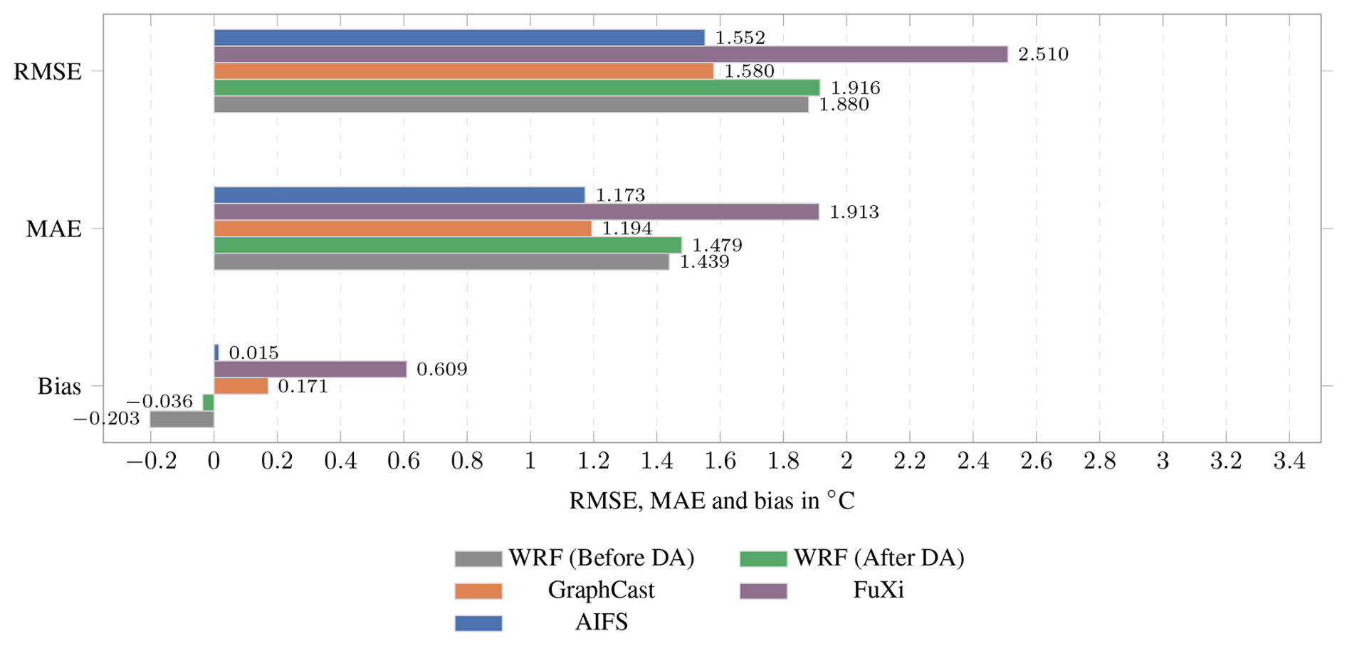
Figure 7 2 m temperature verification of WRF versus the AI models over the 45 925 common pairs of the 2016, 2018 and 2021 events. Lower RMSE and MAE are better and the bias is best near zero. Paired 95 % intervals on the differences between systems are given in Sect. 6.2.3; against the assimilated WRF the RMSE reductions are 0.364 °C for AIFS and 0.337 °C for GraphCast, whereas the small RMSE change produced by assimilation itself (+0.036 °C) is not resolved.

We use a moving-block bootstrap over whole analysis cycles (Gilleland, 2020). The resampling unit is a 6-hourly valid time with all its stations attached. Consecutive cycles are sampled in blocks within each event, retaining the joint spatial field and within-block temporal dependence; dependence is broken at joins between sampled blocks. Every system receives the same resampled cycles. Pooled scores are recomputed from the summed contingency counts or temperature error sums, and 95 % percentile intervals are computed directly for paired differences. We use 10 000 resamples at each of $L=\mathrm{1},\mathrm{2},\mathrm{4},\mathrm{8}$ cycles (6–48 h), with fixed seed 20 260 905. The values below use L=4; all block lengths, individual-model intervals and paired differences accompany the paper. The samples contain 92 119 precipitation pairs and 45 925 temperature pairs per model, with identical station-time keys and observations across systems. Temperature uses the screened subsets of 119, 134 and 148 stations in 2016, 2018 and 2021, respectively.

At 1 mm (6 h)⁻¹, GraphCast exceeds WRF (After DA) in CSI by +0.035 (+0.012 to +0.057), and AIFS by +0.026 (+0.003 to +0.050). Both intervals exclude zero at every block length tested. GraphCast and AIFS are not separated: their difference is +0.009 (−0.003 to +0.020).

At 20 mm (6 h)⁻¹, WRF (After DA) exceeds GraphCast by +0.046 (+0.009 to +0.096), with zero excluded at all four block lengths. Its advantage over AIFS is +0.019 (+0.002 to +0.046), but zero is excluded only for 24 and 48 h blocks. The 6 and 12 h intervals are −0.007 to +0.051 and −0.003 to +0.050, respectively. Thus WRF has the highest point estimate, while its separation from AIFS is sensitive to block length. Overlapping individual-model intervals are not themselves a test of a paired difference.

For temperature, AIFS minus WRF (After DA) RMSE is −0.364 °C (−0.423 to −0.315), and GraphCast minus WRF is −0.337 °C (−0.392 to −0.293). AIFS minus GraphCast is −0.028 °C (−0.041 to −0.011). All three differences exclude zero at every tested block length, and they are the largest well-resolved differences in the study. Assimilation itself changes temperature RMSE by +0.036 °C (−0.008 to +0.083), an interval that contains zero at every tested block length, while moving the signed bias towards zero by +0.167 °C (+0.115 to +0.222), which is resolved at every block length. The analysis therefore improves the mean level of the near-surface temperature field, whereas its effect on the scatter is not resolved by this sample (Fig. 5).

The assimilation effect on CSI at 1 mm is +0.0246. Its interval narrowly excludes zero for independent cycle resampling (+0.0004 to +0.0501), but includes zero at 12, 24 and 48 h; the 24 h interval is −0.0005 to +0.0543. The pooled CSI decreases at 5 and 10 mm, −0.018 and −0.023, also have intervals containing zero at every tested block length, as does the 20 mm change. Across events, the 1 mm CSI increase and the 10 mm decrease have consistent signs; the 5 and 20 mm changes do not. These statements concern CSI: some other diagnostics, including the 1 mm POD increase, exclude zero.

These are conditional, pointwise uncertainty intervals for the three sampled episodes, not simultaneous tests over all model, metric and threshold comparisons. Block-length sensitivity is reported rather than selecting a length to obtain a desired separation. The bootstrap cannot supply additional independent events; generalisation to flood events in general remains limited by the three-event design. FuXi forecasts no 20 mm exceedances in this sample, so its FAR is undefined and has no interval.

6.2.4 Skill by event

Because the three events hold different positions relative to each AI model's training period, the pooled scores are broken down by event in Fig. 8. The 2016 event lies inside GraphCast's training period (1979–2017) and inside FuXi's validation years: FuXi is trained on 1979–2015, validated on 2016–2017 and tested on 2018 (Chen et al., 2023); the 2021 event is entirely unseen by GraphCast and FuXi; for AIFS, all three events fall within its 2016–2022 fine-tuning window.

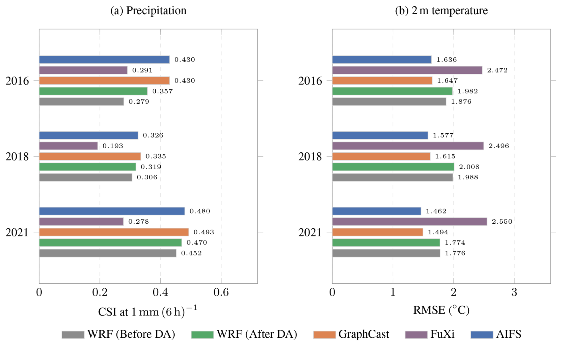
Figure 8 Verification by event on the independent network. (a) Critical Success Index for precipitation at the 1 mm (6 h)⁻¹ threshold, scored on the 12 km-screened network of each event: 259 stations in 2016 (where the archived WRF also ends on 6 August), 280 in 2018 and 264 in 2021; (b) root-mean-square error of 2 m temperature on the screened temperature subset, 119 stations in 2016, 134 in 2018 and 148 in 2021 – the stations of each event's network that also report 2 m temperature. Higher is better in (a), lower in (b). Full scores, including POD, FAR, ETS and bias, are given in the data files accompanying this paper.

The per-event breakdown is broadly stable: GraphCast and AIFS lead in every event, WRF (After DA) is third in every event, and FuXi is last in 2018 and 2021. The ordering is not identical throughout, however. In 2016 AIFS and GraphCast are effectively tied (0.430 against 0.430) and FuXi (0.291) exceeds the unassimilated WRF (0.279), so the pooled ranking should not be read as holding event by event. Notably, GraphCast's categorical skill is highest for the fully out-of-sample 2021 event (CSI 0.493 vs. 0.430 for the in-training 2016 event). This is evidence of useful skill on an event after the training cutoff and tempers the concern that AI models' skill merely reflects memorisation of training samples. It does not identify meteorology as the cause: event difficulty, rainfall prevalence, station composition and observation availability all differ between the events, and CSI itself depends on the occurrence distribution. We note also that 2018 lies after GraphCast's cutoff and is its least skilful event, so the pattern is not simply in-training against out-of-training.

This test is, however, only available for GraphCast and FuXi. Because the AIFS Single 1.0 fine-tuning window (2016–2022) encompasses all three case studies, none of the events is out-of-sample for that model, and its performance here cannot be used to distinguish generalisation from familiarity with the period. The AIFS results should therefore be read as potentially optimistic, since the evaluation periods overlap its development data; its performance on unseen events is not assessed here, and we do not claim these scores are a formal upper bound. The generalisation argument above applies to GraphCast and FuXi only. The 2021 event yields the highest categorical skill for four of the five systems, reflecting the large-scale, long-duration character of that episode; FuXi is the exception, scoring slightly lower there (CSI 0.278) than in 2016 (0.291), so its behaviour supports the generalisation argument less clearly than GraphCast's does; the mean 6-hourly biases remain small throughout, so the systematic underestimation of the July 2021 rainfall is expressed not in the mean but in the amplitude of the heaviest accumulations, which Sect. 6.2.5 and 6.3 examine directly.

Figure 9 condenses the categorical precipitation results into a single performance diagram.

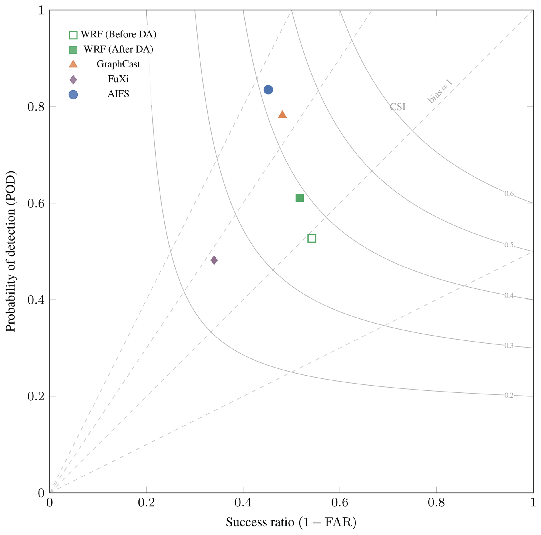
Figure 9 Performance diagram of categorical precipitation skill at the 1 mm (6 h)⁻¹ threshold, computed over the same 92 119 matched pairs for every system. The open square is WRF before assimilation and the filled square WRF after assimilation, so the displacement between them is the effect of the 6-hourly analysis at this threshold. Curved grey lines are constant CSI (0.2–0.6) and dashed grey lines constant frequency bias (0.5, 1, 1.5, 2). Points nearer the top-right corner are more skilful.

6.2.5 Sensitivity to the precipitation threshold

The scores discussed so far use a 1 mm (6 h)⁻¹ threshold, which measures whether a system places rainfall in the right place at the right time but says little about its ability to reproduce rainfall intensity, the property that matters for flash-flood warning. The categorical scores were therefore recomputed at 5, 10 and 20 mm (6 h)⁻¹ (Fig. 10).

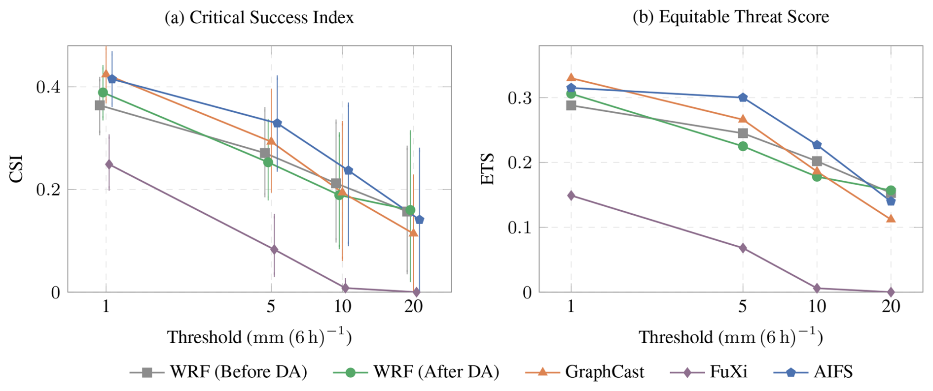
Figure 10 Categorical precipitation skill as a function of exceedance threshold, pooled over the three events on the independent network (92 119 matched pairs). (a) Critical Success Index, with error bars giving the 95 % confidence interval from the moving-block bootstrap with 24 h blocks and 10 000 resamples; the five series are offset by a few per cent in threshold so that the bars remain legible, and the tick labels give the true thresholds. (b) Equitable Threat Score. These are individual-model intervals; comparisons between systems use the paired-difference intervals in Sect. 6.2.3. GraphCast and AIFS lead at 1 mm but fall below WRF by 20 mm, and FuXi produces no exceedance of 20 mm (6 h)⁻¹ anywhere in the verification set. POD, FAR and all confidence intervals are provided in the accompanying data files.

The ranking obtained at 1 mm does not survive the increase in threshold. AIFS, second to GraphCast at 1 mm, has the highest skill at 5 and 10 mm, and at 10 mm it is clearly the best system (CSI 0.237 against 0.189 for the assimilated WRF), but at 20 mm (6 h)⁻¹ the ordering reverses and WRF becomes the most skilful system (CSI 0.160 with assimilation and 0.157 without, against 0.141 for AIFS). The degradation of the two models trained on reanalysis alone is more severe: GraphCast falls from CSI 0.424 at 1 mm to 0.114 at 20 mm, and FuXi does not produce a single exceedance of 20 mm (6 h)⁻¹ anywhere in the verification set. Its POD, CSI and ETS are therefore zero and its false-alarm ratio is undefined, since it forecasts no exceedance to be wrong about.

Including the unassimilated run in Fig. 10 reveals a second feature that the 1 mm scores conceal: the benefit of assimilation is itself threshold-dependent. At 1 mm the analysis raises CSI from 0.364 to 0.389; the paired block bootstrap of Sect. 6.2.3 puts that difference at +0.024, with an interval that excludes zero when cycles are resampled individually but includes it once 24 h blocks are used, so we report the improvement as consistent in this sample rather than as established. At higher thresholds the sign changes. At 10 mm the assimilated run scores marginally lower than the cold-start run (CSI 0.189 against 0.212), and at 5 mm likewise (0.253 against 0.271); at 20 mm the two are indistinguishable (0.160 and 0.157). The degradation at 10 mm is present in all three events but is largest for the 2018 Mullerthal case (−0.027), against −0.009 for 2021 and −0.008 for 2016. The differences are small in absolute terms, and we do not claim that any single event carries the pooled signal.

The three events differ substantially in what was available to assimilate (Table 4). The 2021 analysis ingests roughly 3200 reports per cycle, including 215 GNSS ZTD retrievals and about 1600 aircraft profiles, whereas the 2016 and 2018 analyses ingest about a third of that volume, dominated by satellite atmospheric motion vectors, with fewer than 35 ZTD retrievals per cycle and no aircraft data. The contrast is starker in the GNSS network itself: 232 distinct ZTD sites are assimilated somewhere in the domain during the 2021 window, against 33 in 2016 and 29 in 2018, and within Luxembourg 9 against one in each of the earlier events. This difference reflects what the observing system delivered rather than a design choice, since aircraft coverage depends on commercial traffic and the denser 2021 GNSS network was assembled from regional providers whose archives do not extend to the earlier events. We record these counts for completeness, but they do not explain the high-threshold behaviour: the degradation at 10 mm is of similar size in the densely observed 2021 event (−0.009) and in the sparsely observed 2016 event (−0.008).

The contingency tables show what form the degradation takes. For 2018 at 10 mm the unassimilated run converts 132 of its heavy forecasts into hits against 114 for the assimilated run, on a sample containing 900 observed exceedances. The number of heavy forecasts rises from 263 to 338 while the hits fall from 132 to 114, so the assimilated run issues more heavy forecasts and gets fewer of them right. That is a statement about exceedance counts; it does not by itself establish that a comparable volume of rain was placed in the wrong locations, which would require a displacement analysis. The frequency bias for that event moves the same way: at 10 mm it is 0.29 before assimilation and 0.38 after, so both configurations under-forecast the number of heavy events. A fuller attribution would require the observation-minus-background and observation-minus-analysis statistics of each cycle, which were not retained for these experiments and which we recommend archiving in any repetition of this work.

We draw no causal conclusion from this. With three events, observation density, observation type and synoptic character cannot be separated, and the high-threshold behaviour is in any case not ordered by observation density. Establishing why assimilation fails to improve intensity would require repeating a single event with its observation set systematically varied while the meteorological situation is held fixed. We identify this as the natural next step rather than a result of the present study.

Two checks nevertheless constrain the interpretation. First, AIFS, which shares no component with the WRF chain, converts 131 of its 243 heavy forecasts into hits for the same event, so the 2018 rainfall was to some degree predictable at this threshold; that makes a pure artefact of the verification network less likely, though it does not exclude one. Second, the 2018 analyses ingest the full surface observing network, so the high-threshold behaviour is not a consequence of a depleted observation set. One interpretation is that surface pressure, wind and screen-level observations alone do not supply the mid-tropospheric moisture information these convective cases require; we offer it as a hypothesis, since the experiment repaired the observation set rather than denying one observation type in a controlled way. The practical statement we are willing to make is therefore a narrow one: assimilation improved the detection of rainfall occurrence in all three events, and lowered the pooled CSI at 5 and 10 mm (6 h)⁻¹, with the 10 mm decrease present in every event. It is not a uniform degradation at intensity: the 5 mm score improves in 2016 (0.168→0.198) and the 20 mm score improves in 2021 (0.227→0.278), and pooled over the three events the 20 mm CSI is marginally higher after assimilation (0.157→0.160). The size of the 10 mm shortfall is not ordered by how densely each event was observed. CSI at a threshold combines occurrence, threshold crossing and placement, so these are not pure measures of intensity. We note that exceedances of the highest threshold are rare in each individual event (323 observed exceedances of 20 mm in 2018, for example, out of 33 999 pairs), so the per-event attribution should be read as indicative rather than conclusive.

This behaviour is the quantitative counterpart of the spatial fields discussed in Sect. 6.3. Models trained with pixel-wise loss functions are rewarded for predicting the conditional mean, which suppresses the extremes of the distribution; the resulting fields are spatially smooth and rarely attain high 6 h accumulations. The practical implication is that the apparent advantage of the AI systems at low thresholds should not be extrapolated to the rainfall rates that generate flash floods, and that a physics-based model with observation correction remains the more reliable source of intensity information at those rates.

6.2.6 Skill restricted to the flood days

The scores presented so far are computed over the full evaluation windows. To isolate performance during the extreme episodes themselves, they were recomputed using only the 6 h periods spanning each flood (21–23 July 2016, 31 May–2 June 2018, and 13–15 July 2021), giving 9600 matched pairs in total (Fig. 11).

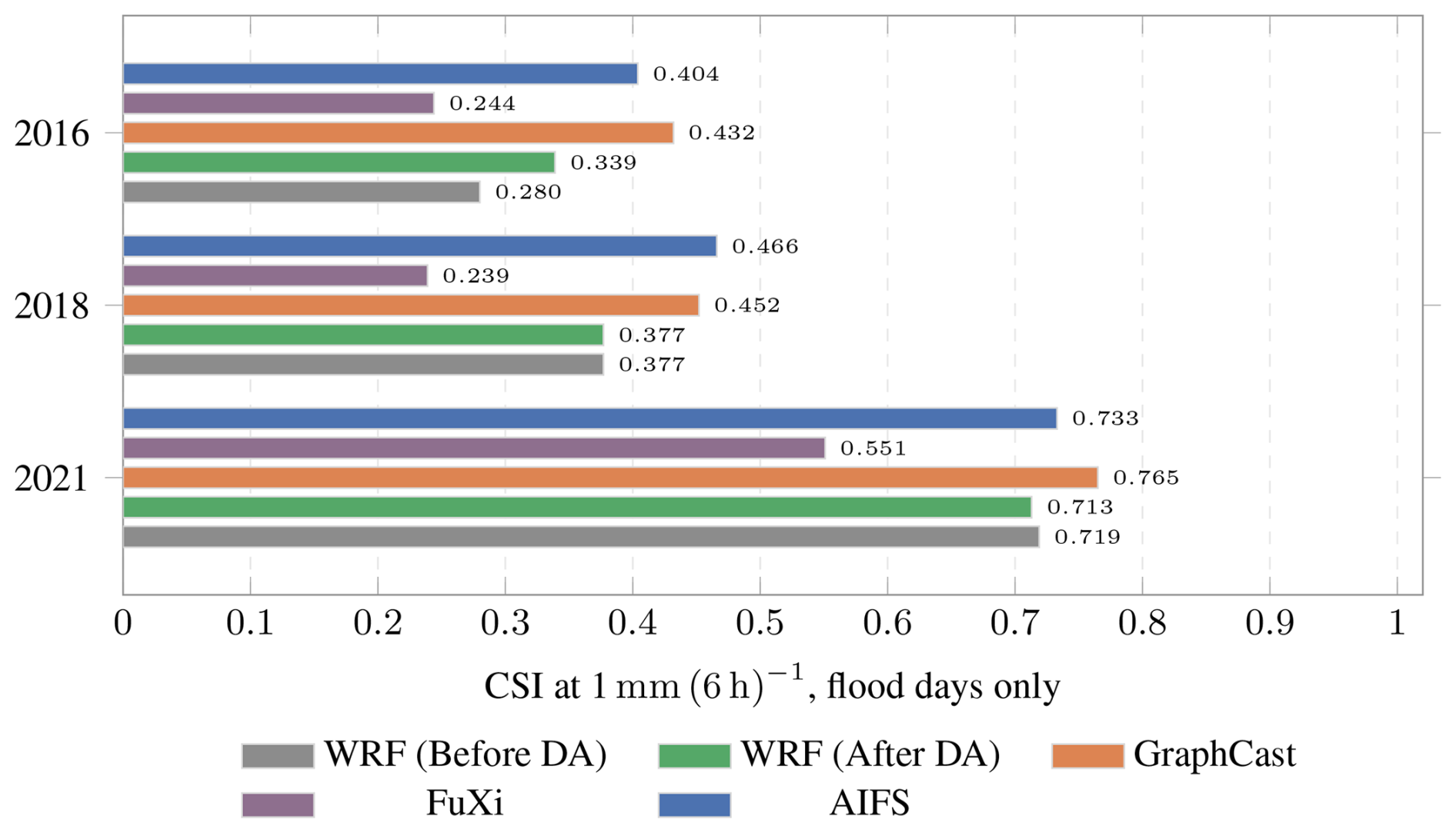
Figure 11 Critical Success Index restricted to the flood days alone (21–23 July 2016, 31 May–2 June 2018, 13–15 July 2021), on the same 12 km-screened networks used for the full windows. Pooled over the three events this subset contains 9600 matched pairs against 92 119 for the full windows. Scores are markedly higher during the flood days in 2018 and 2021, where rainfall is widespread and persistent; in 2016, the weakest of the three episodes, three of the five systems score slightly lower on the flood days than over the full window. The two leading AI systems remain ahead of WRF, although AIFS overtakes GraphCast in 2018 and the two WRF configurations change places in 2018 and 2021 by margins of 0.0005 and 0.006, so the full-window conclusions are not an artefact of including quiescent days.

Scores are markedly higher during the flood days in 2018 and 2021, which is expected: rainfall is widespread and persistent during these episodes, so the detection problem is easier than it is for the scattered convection of the intervening fair-weather periods. In 2016, the weakest of the three episodes, three of the five systems score slightly lower on the flood days than over the full window. GraphCast and AIFS remain ahead of both WRF configurations in every event, but they change places: AIFS leads narrowly in 2018 (0.466 against 0.452), whereas GraphCast is ahead in that event over the full window (0.335 against 0.326).

Two qualifications. The two WRF configurations also change places, the assimilated run falling behind the cold start on the flood days of 2018 and 2021 while remaining ahead over all three full windows; the margins are too small to carry weight, 0.0005 in 2018 (0.3770 against 0.3765, indistinguishable at the precision plotted) and 0.006 in 2021. And this test is made at 1 mm (6 h)⁻¹ only, so it does not establish that the 20 mm ordering of Sect. 6.2.5 survives restriction to the flood days. Two features are specific to the events. First, the mean biases turn markedly more negative: pooled over the flood days they run from −0.28 mm for AIFS to −2.07 mm for FuXi, against near-zero values over the full windows, so the underestimation is confined to the heavy-rainfall periods, exactly as the threshold analysis of Sect. 6.2.5 implies. Second, during the July 2021 flood the WRF configurations achieve the lowest false-alarm ratios recorded anywhere in this study (0.093 before assimilation and 0.130 after, against 0.207 for GraphCast and 0.255 for AIFS), indicating that when the regional model predicts rainfall during such an episode it is almost always correct, even though it detects fewer of the events than the AI systems (POD 0.798 against 0.956 for GraphCast).

6.3 Event-scale evaluation: the July 2021 flood

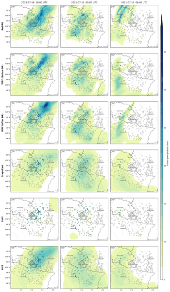
The aggregated scores are complemented by a spatial evaluation against the Belgian weather-radar composite for the peak of the July 2021 flood. Hourly RADFLOOD21 radar accumulations (Goudenhoofdt et al., 2023) were aggregated to 6 h windows. This evaluation is restricted to 2021 because RADFLOOD21 was released specifically for this event, whereas no equivalent open radar product covers 2016 and 2018. Figure 12 compares the 6 h precipitation fields at three consecutive timestamps spanning the event peak (14 July 18:00 UTC to 15 July 06:00 UTC).

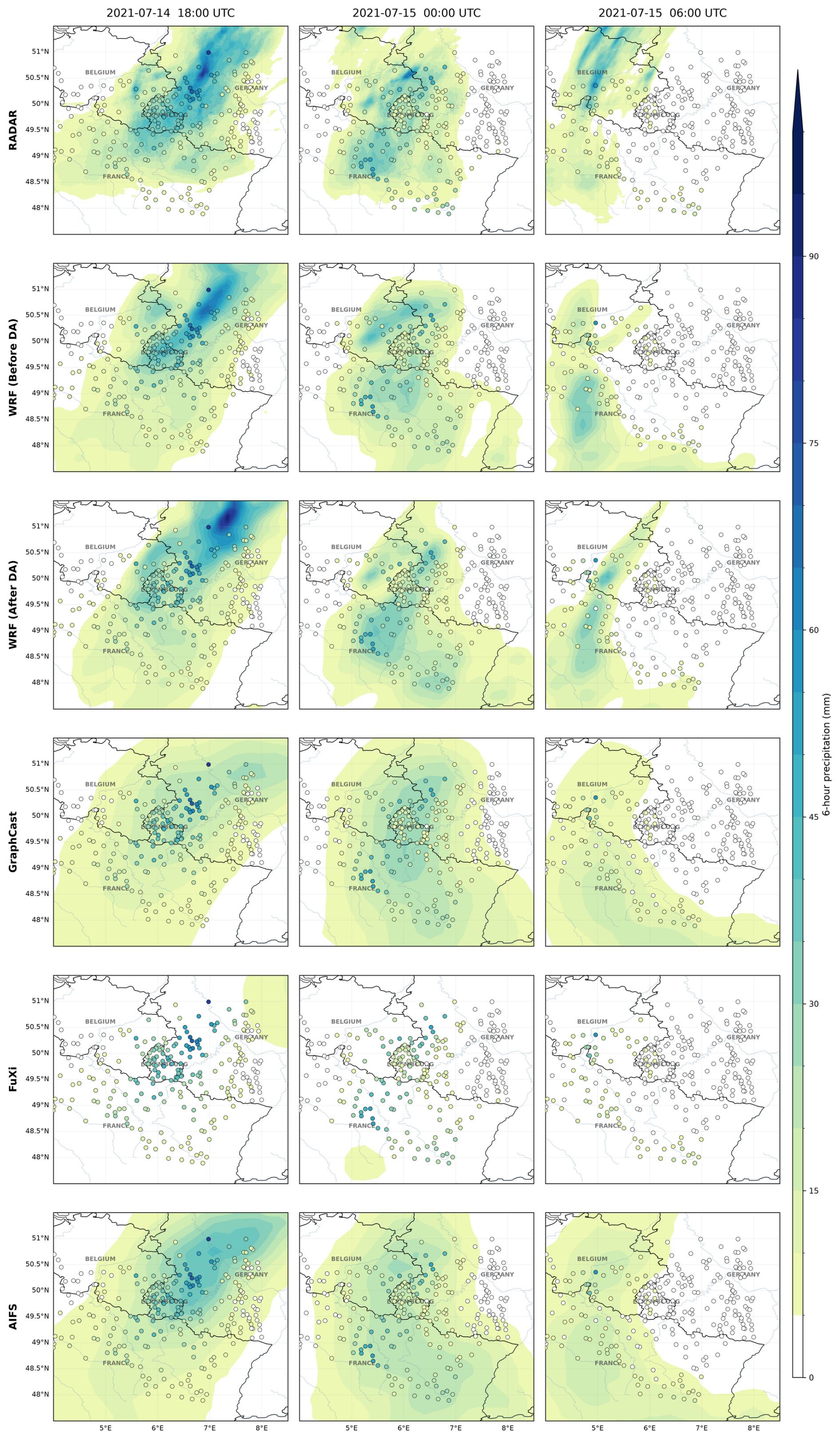
Figure 12 6 h precipitation fields over Luxembourg and the Greater Region at the peak of the July 2021 flood (columns: valid 14 July 2021 18:00 UTC, 15 July 2021 00:00 UTC, and 15 July 2021 06:00 UTC). Rows show the Belgian radar composite, WRF before and after data assimilation, GraphCast, FuXi, and AIFS. All model fields are 6 h forecasts initialised 6 h before the valid time; the shared colour scale gives the 6 h accumulation in mm. Filled circles show the gauge observations of the independent verification network at the same valid times, plotted on the same colour scale so that station, radar and model values can be compared directly.

The station gauges overlaid on each panel provide a partial check on the radar composite: within Luxembourg the two agree closely on both the location and the magnitude of the heaviest 6 h accumulations. That check is weaker than it may appear. RADFLOOD21 is a radar–gauge merged analysis whose inputs include the Belgian SPW network, so the SPW gauges in our verification set are not independent of it; the Luxembourg AgriMeteo gauges are, and it is those that support the agreement quoted here. Agreement at a few stations also does not validate the composite across the whole scoring domain – at Mirecourt, near the edge of the composite, the radar gives 42.3 mm against 62.0 mm at the gauge. We therefore treat the radar as a useful spatial reference rather than as ground truth.

Including the unassimilated WRF run in the comparison isolates the effect of the assimilation on the spatial field, and here the visual impression and the quantitative score disagree, so we report both. Both configurations place the rain band in approximately the correct position and the assimilated field looks the sharper of the two. Scored against the radar over these three panels alone, however, the unassimilated run is the better of the two at every threshold and every neighbourhood width, and its spatial correlation with the radar accumulation is higher (0.671 against 0.578); at the 12 km neighbourhood and the 1 mm (6 h)⁻¹ threshold it attains an FSS of 0.849 against 0.801, using the same kilometre-sized neighbourhoods and native-to-common-grid treatment as Sect. 6.4. Over the full week (Sect. 6.4) the ordering is the opposite at the lower thresholds, where assimilation raises the panel-mean FSS from 0.502 to 0.519 at 1 mm and from 0.366 to 0.385 at 5 mm at 12 km, and raises correlation from 0.290 to 0.306. These are descriptive differences; the pooled FSS can rank the two WRF configurations differently, and no dependence-aware uncertainty analysis of radar FSS is presented here. The peak and week summaries therefore need not support identical statements about assimilation. We draw attention to this because it also illustrates why the visual comparison of Fig. 12 cannot stand on its own, and why the quantitative scores of Sect. 6.4 are reported alongside it.

The radar shows an intense, elongated rain band stretching from Belgium across Luxembourg into western Germany. Both WRF configurations reproduce this banded mesoscale structure and its sharp gradients, and the assimilated field looks the sharper of the two, although as reported above the cold-start run scores higher over these three panels. GraphCast captures the correct location of the rainfall envelope but is strongly smoothed and underestimates peak intensities. FuXi produces almost no precipitation signal during the peak, consistent with its poor categorical scores. AIFS produces the largest and most coherent precipitation envelope of the three AI systems, which explains its high detection rates, but its fields remain smooth and broad relative to the radar. Thus, even where the aggregated skill of AIFS or GraphCast matches or exceeds WRF, the physics-based model retains a clear advantage in representing the fine-scale structure and amplitude of extreme convective rainfall.

Figure 13 shows 6-hourly precipitation time series from 10 to 17 July 2021 at four illustrative stations near the verification network described in Sect. 5.3. Three span the physiographic gradient of the study area described in Sect. 2: Briedfeld in the northern Oesling, Ettelbruck near the Sauer–Alzette confluence, and Oberkorn in the southern Gutland. Mirecourt lies some 150 km to the south in France and tests behaviour away from the core catchments. Briedfeld passes the 12 km separation screen but fails the 95 % completeness rule, so it is not included in the pooled verification sample.

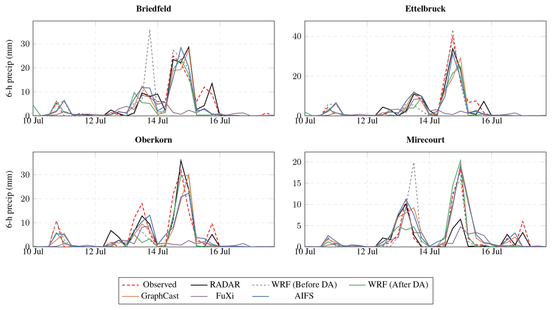
Figure 13 Six-hourly precipitation time series for 10–17 July 2021 at four independent gauges: Briedfeld in the northern Oesling, Ettelbruck near the Sauer–Alzette confluence and Oberkorn in the southern Gutland, all in Luxembourg, and Mirecourt some 150 km south in France as a distant control. Plotted are the gauge observations, the Belgian radar estimate, WRF before and after data assimilation, GraphCast, FuXi and AIFS. Model values are 6 h forecasts valid at each time, sampled at the nearest grid point to the station; gaps indicate periods without radar coverage. Ettelbruck, Oberkorn and Mirecourt belong to the screened verification network of Sect. 5.3; Briedfeld lies 40 km from the nearest assimilated observation and so passes the independence screen, but its 30 d record does not meet the 95 % completeness rule and it is therefore not part of the scored network.

The time series corroborate both the aggregated metrics and the spatial analysis. At the three Luxembourgish stations the gauge and radar records agree closely on the timing and magnitude of the episode (130.6, 121.8 and 131.8 mm at the gauges against 129.3, 116.2 and 116.3 mm from the radar over the 8 d window), providing a well-constrained target against which the forecasts can be judged. Of the systems plotted, the unassimilated WRF comes closest at Briedfeld (134.5 mm against 130.6 mm observed) while AIFS is closest at the other two (112.0 and 113.0 mm; 121.4 mm at Briedfeld), and AIFS captures the timing of the heaviest 6 h accumulations; GraphCast is close behind at all three (113.7, 106.5 and 100.4 mm); the assimilated WRF follows with somewhat weaker peaks (97.9, 87.5 and 94.5 mm); and FuXi remains far too low throughout the episode (56.0, 48.8 and 42.5 mm), less than half the observed total at every station, consistent with its poor categorical scores. At Mirecourt, where the event was much weaker, the ordering differs: WRF tracks the observed total most closely (60.5 mm against 62.0 mm observed) whereas AIFS overestimates it (89.6 mm), indicating that the tendency of AIFS to produce broad, coherent precipitation envelopes helps it during widespread heavy rainfall but costs accuracy in more marginal situations.

6.4 Spatial verification against radar

The comparison in Sect. 6.3 is visual, and visual comparison of precipitation fields is subjective. The week covered by the radar composite was therefore scored quantitatively using the Fractions Skill Score (FSS; Roberts and Lean, 2008), which compares the fraction of grid points exceeding a threshold within a neighbourhood of increasing size and so credits a forecast that places rainfall approximately, rather than exactly, in the right place.

Four points of sampling and method are stated explicitly, because each of them can move the scores. First, a 6 h radar total is formed only where all six hourly composites exist; a partial window is discarded rather than treated as containing dry hours. Of the 28 6 h periods of 11–17 July 2021 this removes one, 11 July 00:00 UTC, for which only the final hour is archived. Second, the systems are scored on the intersection of the valid times at which the radar and every system has a field, which leaves 27 common periods, 11 July 06:00 to 17 July 18:00 UTC. Third, all fields reach the common mesh by the same nearest-neighbour step from their own native grids: the 0.02° (∼ 2.2 km) mesh spanning 47.5–51.5° N and 4.0–8.5° E. Inside that box the native grids provide 1764 points for WRF, 323 each for GraphCast and FuXi, and 159 for AIFS on its N320 reduced Gaussian grid, so AIFS is the most coarsely sampled of the systems compared here, not the least. Fourth, a period in which neither the forecast nor the radar exceeds the threshold carries no information and cannot be scored; such periods are excluded, so the number of scored periods falls as the threshold rises, from 25–27 at 1 mm to 18 at 20 mm (6 h)⁻¹. Those counts, and a pooled aggregate FSS formed from summed numerator and denominator terms over the common periods, are given in the data file accompanying this paper; the aggregate weights panels by their FSS denominator and can change the ordering. At 1 mm and 12 km, for example, GraphCast leads the aggregate (0.748), ahead of WRF Before DA (0.738), WRF After DA (0.732) and AIFS (0.730), whereas AIFS leads the panel mean. At 100 km the aggregate leader is WRF Before DA (0.874). At 20 mm, both estimators place WRF ahead of the AI models, although their preferred WRF configuration differs at 100 km. Rankings must therefore name the estimator. Neighbourhood filtering uses zero padding outside the rectangular scoring domain.

Results are given in Fig. 14, together with the spatial correlation of the 6 h accumulation fields.

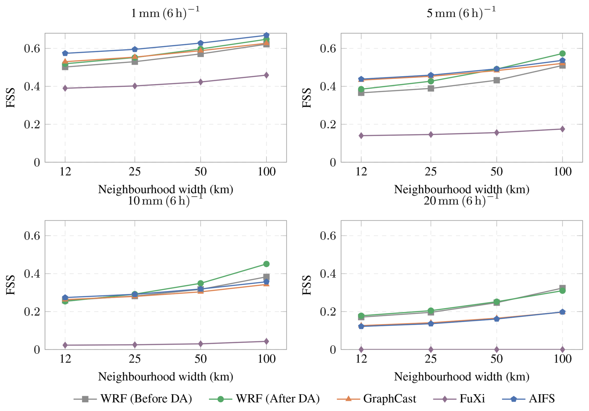
Figure 14 Fractions Skill Score against the RADFLOOD21 radar composite over the 27 six-hourly periods of 11 July 06:00 to 17 July 18:00 UTC for which the radar total is complete and every system has a field, as a function of neighbourhood width, at four exceedance thresholds. Higher is better. The neighbourhood is sized in true kilometres in both directions on the common 0.02° mesh, and every field reaches that mesh by the same nearest-neighbour step from its native grid. Periods with no exceedance in either field are unscorable and excluded, so the number of scored periods falls with threshold (25–27 at 1 mm, 18 at 20 mm); the per-threshold counts and a pooled aggregate FSS are in the accompanying data file. AIFS leads the panel mean at 1 mm at every width, and at 5 mm at 12–50 km; WRF After DA leads at 5 mm and 100 km (0.573 against 0.537 for AIFS). The ordering reverses with intensity and at 20 mm (6 h)⁻¹ the two WRF configurations are ahead of all three AI models. All three global models are coarser than the 12 km neighbourhood – 323 native points for GraphCast and FuXi and 159 for AIFS inside the scoring box, against 1764 for WRF – so the 12 km column is below the scale any of them resolves. Spatial correlations with the radar field are 0.290 (WRF Before DA), 0.306 (WRF After DA), 0.410 (GraphCast), 0.081 (FuXi) and 0.414 (AIFS).

The quantitative scores show the same threshold dependence as the station scores. At 1 mm (6 h)⁻¹ AIFS leads the panel mean at every neighbourhood width (0.574 at 12 km), ahead of GraphCast (0.530), the assimilated WRF (0.519) and the cold-start run (0.502); at 5 mm AIFS leads at 12–50 km, while WRF After DA leads at 100 km (0.573 versus 0.537). The ordering reverses as intensity increases. At 20 mm (6 h)⁻¹ a WRF configuration is the most skilful system at every width: the assimilated run leads at 12, 25 and 50 km (0.178 at 12 km) and the cold-start run at 100 km (0.324 against 0.310). At 12 km GraphCast and AIFS attain 0.126 and 0.122, and at 100 km 0.197 and 0.198, while FuXi produces no exceedance anywhere in the scored periods. FSS is non-decreasing with neighbourhood width in these results. This alone does not distinguish amplitude from displacement errors; the amplitude statistics provide separate evidence of peak attenuation. The spatial correlation of the 6 h accumulation fields runs the other way at all thresholds – 0.414 (AIFS), 0.410 (GraphCast), 0.306 (WRF After DA), 0.290 (WRF Before DA), 0.081 (FuXi) – so the AI fields track the broad pattern of the accumulation more closely even where they fail to reproduce its extremes.

Two caveats apply. All three global models are coarser than the 12 km neighbourhood – GraphCast and FuXi at 0.25° and AIFS on N320, giving 323, 323 and 159 native points inside the scoring box against 1764 for WRF – so that column lies below the scale any of them resolves and none of the three is exempt from the limitation. Whether a sub-grid neighbourhood score is a strict lower bound on what the model could achieve is not established, and we do not claim it. And although the sample spans 27 6 h periods, they all fall within a single week of one event, so these values characterise this flood episode rather than model behaviour in general.

6.5 Effect of horizontal resolution

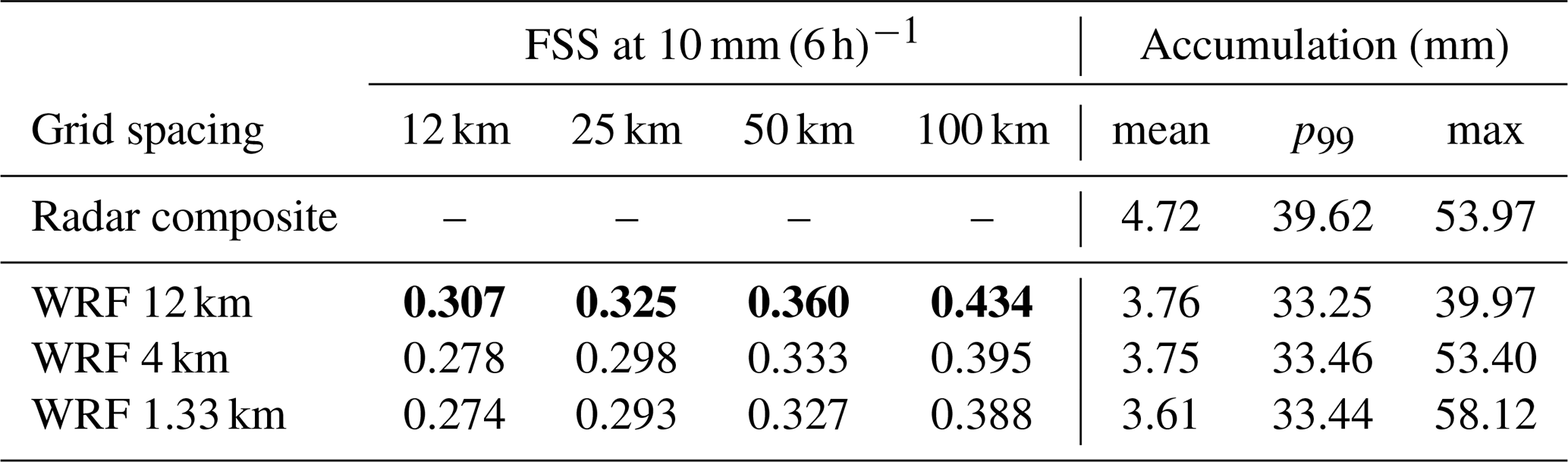
The comparison above sets a 12 km limited-area model against global systems at 25–28 km, and it is reasonable to ask whether the advantage of WRF follows from its finer grid rather than from its formulation. The 12 km domain used throughout this study is the outermost member of a 12–4–1.33 km nest configured following the recommended 1:3 ratio, the innermost member of which is intended to drive hydraulic simulation of the Luxembourgish catchments at approximately 1 km. That nest was integrated from 12 July 12:00 to 17 July 18:00 UTC, which allows the question to be addressed directly, although only for those 22 6 h periods and only over the footprint of the innermost domain (49.2–50.1° N, 5.6–7.0° E). The three nest members were scored against the radar composite exactly as in Sect. 6.4 (Table 5).

Table 5 Effect of horizontal resolution. FSS against the radar composite over the footprint of the innermost domain, on the 22 six-hourly periods of 12 July 12:00 to 17 July 18:00 UTC for which the radar total is complete and all three nest members exist. The nest was not integrated before 12 July 12:00, so this is a shorter sample than the 27 periods of Sect. 6.4; radar and all three members are scored on exactly these periods and on identical geography. Accumulation columns are the domain mean, 99th percentile and maximum 6 h total over the same 22 periods. Bold indicates the highest FSS in each column.

The nest is run with two-way feedback, so the inner domains are not passive receivers: the solution on each nest is communicated back to its parent at every coupling step, and the analysis increment introduced on the 12 km domain is therefore propagated through all three members. Assimilating the same reports separately on the finer grids would reuse observations that have already been applied on the parent domain, which would count the same information twice rather than add new constraint. The comparison in this section is consequently a test of horizontal resolution at fixed analysis, which is the quantity in question. Assimilation performed directly at convection-permitting scale is a different experiment, requiring observation error statistics and a background error covariance appropriate to that scale, and we identify it as future work.

Refining the grid does not improve the position-based scores. FSS at 10 mm (6 h)⁻¹ falls from 0.307 at 12 km to 0.278 at 4 km and 0.274 at 1.33 km, and the spatial correlation declines in the same order (0.145, 0.135, 0.106). This is consistent with the double-penalty behaviour familiar from convection-permitting verification, in which a finer model generates sharper and more numerous small-scale features and any displacement of them is penalised twice, once as a miss and once as a false alarm. We offer that as the likely explanation rather than a demonstrated one: FSS responds to coverage and amplitude as well as to displacement, and separating them would require object-based displacement diagnostics or matched-smoothing experiments that we have not performed.

The amplitude statistics move in the opposite direction, but only in the tail. The maximum 6 h accumulation rises from 39.97 mm at 12 km to 53.40 mm at 4 km and 58.12 mm at 1.33 km, against the 53.97 mm recorded by the radar over the same periods: the 12 km domain falls well short of the observed peak, the 4 km domain reaches it almost exactly, and the 1.33 km domain exceeds it by some 8 %. The bulk of the distribution does not follow. All three members carry a domain-mean 6 h total of 3.6–3.8 mm against 4.72 mm from the radar, so every member is 20 %–24 % low in the mean and refinement does not close that gap; the 99th percentile is likewise flat across the three at 33.2–33.5 mm against 39.62 mm observed. The finer nests therefore do what convection-permitting simulation is expected to do for the heaviest cells – to the point of slight overshoot at 1.33 km – while leaving a persistent deficit in the bulk of the accumulation and being scored more harshly by neighbourhood metrics.

What this experiment can and cannot settle should be stated carefully. It shows that within WRF, refining the grid by an order of magnitude raises peak accumulation but does not raise the neighbourhood scores: from 12 to 1.33 km the 10 mm score at the 12 km neighbourhood changes by −0.033 (0.307 to 0.274). It does not test WRF against the AI systems at a matched 25–28 km grid, which is the comparison that would isolate resolution in the cross-model difference, and a non-monotonic response within one model does not by itself exclude a role for grid spacing between models. The two experiments also use different geography and different samples: the wide domain over 27 periods in Sect. 6.4, the inner footprint over 22 here. For scale, at 10 mm and the 12 km neighbourhood the spread between WRF and the two stronger AI systems in Fig. 14 is 0.020 (0.254–0.274), smaller than the 0.033 produced by refinement within WRF; the much larger spread across all systems depends on including FuXi. What can be said is that the AI fields do not reach the observed intensities at any scale, whereas the WRF nest attains and slightly exceeds the observed peak once the grid is refined to 4 km and below. Resolution contributes to the sharpness of the WRF fields, as acknowledged in Sect. 7; whether it is also the origin of the contrast between the two modelling paradigms is not resolved by this experiment.

7 Conclusions

This study benchmarked an observation-corrected WRF configuration against three state-of-the-art AI weather models (GraphCast, AIFS, and FuXi) across three high-impact flood events (2016, 2018, and 2021) over Luxembourg and the Greater Region, verifying precipitation and 2 m temperature over 90 simulation days per system against a four-country station network independent of the assimilated observations (259, 280 and 264 precipitation stations in 2016, 2018 and 2021; 92 119 matched precipitation pairs). Several main conclusions emerge. First, 6-hourly 3D-VAR assimilation of conventional and GNSS ZTD observations raises WRF's categorical precipitation skill at the 1 mm threshold (CSI 0.364 to 0.389) and brings the near-surface temperature bias close to zero. The temperature bias change is resolved by the paired block bootstrap (+0.167 °C, +0.115 to +0.222); the precipitation improvement is not once 24 h blocks are used, and should be read as the behaviour of this sample. The benefit is in any case confined to light rainfall: at 10 mm (6 h)⁻¹ the assimilated run scores lower than the cold-start run. The degradation appears in all three events (−0.008 in 2016, −0.027 in 2018 and −0.009 in 2021) and is not ordered by the density of the assimilated observing network: the densely observed 2021 event degrades as much as the sparsely observed 2016 one. We therefore report it without attributing a cause. The practical statement is narrow: assimilation improved where rain falls in every event, and lowered the pooled score at 5 and 10 mm (6 h)⁻¹. The effect is not uniform across events and thresholds – 2016 improves at 5 mm and 2021 at 20 mm, and the pooled 20 mm score is marginally higher after assimilation – so we report a threshold-dependent effect rather than an absence of benefit at intensity. Establishing why would require repeating a single event with its observation set varied systematically, which we identify as the priority for future work. Second, at the 1 mm (6 h)⁻¹ threshold GraphCast and AIFS both detect rain far better than the regional model – AIFS reaches the highest detection rate (POD 0.835) and GraphCast follows at 0.782, against 0.611 for the assimilated WRF – and GraphCast attains the highest overall net skill (CSI 0.424), marginally ahead of AIFS (0.415; the two are not separated by the paired bootstrap) and ahead of WRF by +0.035 (+0.012 to +0.057), which is resolved. Both WRF configurations nevertheless keep lower false-alarm ratios (0.458 before assimilation, 0.483 after) than any AI system. Third, GraphCast and AIFS surpass WRF and FuXi for temperature forecasting, reducing RMSE by 19.0 % and 17.6 % respectively; these are the largest and most securely resolved differences in the study, the paired intervals against the assimilated WRF being −0.364 (−0.423 to −0.315) °C for AIFS and −0.337 (−0.392 to −0.293) °C for GraphCast. Assimilation itself improves the temperature bias (+0.167, +0.115 to +0.222, resolved) while its effect on temperature RMSE (+0.036, −0.008 to +0.083) is not resolved by this sample. Fourth, the per-event breakdown (Fig. 8) shows no skill degradation for GraphCast on the out-of-sample 2021 event – its skill is in fact highest there – showing useful skill after its training cutoff without isolating the effects of meteorology, sampling or training-data overlap. The evidence is not one-sided: 2018 also lies after GraphCast's cutoff and is its weakest event, so the pattern is not simply in-training against out-of-training. FuXi scores marginally lower in 2021 than in 2016, so this evidence rests mainly on GraphCast.

The fifth and most consequential conclusion is that this ordering depends on the rainfall rate considered. As the exceedance threshold is raised the advantage of the data-driven models disappears: at 20 mm (6 h)⁻¹ WRF has the highest CSI point estimate (CSI 0.160 with assimilation and 0.157 without), AIFS falls to 0.141, GraphCast to 0.114 and FuXi produces no exceedances whatsoever. Small pooled mean biases do not establish an accurate upper tail because compensating errors can cancel. The observed reduction in high-threshold skill is consistent with smoothing from mean-oriented training losses, but this experiment does not isolate that mechanism. The radar comparison for July 2021 shows the same effect in space, and the Fractions Skill Score makes it quantitative: over the 27 six-hourly periods for which the radar total is complete and every system has a field, AIFS leads the panel-mean FSS at 1 mm (6 h)⁻¹ at every neighbourhood width (0.574 against 0.530 for GraphCast and 0.519 for the assimilated WRF at 12 km), but the ordering reverses with intensity and at 20 mm (6 h)⁻¹ a WRF configuration leads at every width (assimilated 0.178 at 12 km versus 0.126 for GraphCast and 0.122 for AIFS; cold-start 0.324 at 100 km versus 0.197 and 0.198). These radar scores are a field-to-field comparison and do not involve the station screening. All three global models are coarser than the 12 km neighbourhood – 323 native points for GraphCast and FuXi and 159 for AIFS inside the scoring box – so that column lies below the scale any of them resolves.

Sixth, this structural advantage is not a consequence of horizontal resolution. Refining the WRF grid from 12 to 4 and then 1.33 km over the July 2021 radar week raises the simulated peak 6 h accumulation from 39.97 mm to 53.40 and 58.12 mm, against 53.97 mm observed by radar, as convection-permitting simulation should, but it does not raise the FSS, which falls from 0.307 to 0.274 at 10 mm (6 h)⁻¹ through the familiar double-penalty mechanism. The difference between WRF and the AI systems at a common threshold is therefore larger than the difference resolution produces within WRF itself.

Several caveats temper the apparent superiority of AIFS at low thresholds. All three case-study events lie inside its fine-tuning period, and AIFS inherits information from ECMWF's full operational data-assimilation system, vastly more observations than the conventional and GNSS ZTD network assimilated into WRF. Furthermore, AIFS operates on a coarser grid (∼ 28 km), and its high detection rates partly reflect spatial smoothness that inflates POD at the expense of FAR. A further structural asymmetry should be borne in mind: the three AI systems are global models run at 0.25° or N320 (∼ 25–28 km), whereas WRF is a limited-area model integrated at 12 km. Part of the smoothing evident in the AI precipitation fields is therefore attributable to resolution rather than to the data-driven formulation itself. The 12 km configuration was retained because it is the outermost member of a 12–4–1.33 km nest designed to drive hydraulic simulation of the Luxembourgish catchments, and degrading it to 25 km would not correspond to any configuration of operational interest. Limited-area data-driven models trained specifically for extremes (Xu et al., 2025; Baño-Medina et al., 2025) are a promising route to separating these two effects, and represent a natural continuation of this work.

The AI models produce these forecasts on a single NVIDIA A100 GPU in roughly 15 s per 6 h step, whereas WRF requires approximately 37 min on 52 Intel Xeon cores for the same step including the 3D-VAR analysis, a factor of about 140, underscoring the efficiency of data-driven inference. These results are retrospective 6 h hindcasts re-initialised from reanalysis, not a test of real-time warning performance, and they stop at the rainfall field rather than at discharge. Read with that limit, they suggest a complementary strategy worth testing prospectively: AI models for rapid temperature fields and for detection of rainfall occurrence, and observation-corrected WRF where the heaviest rates matter. The high-threshold advantage is narrow in absolute terms – at 20 mm (6 h)⁻¹ the assimilated WRF has the highest CSI (0.160) but a POD of 0.216 and a false-alarm ratio of 0.619, so it misses most observed exceedances, and AIFS has the lower false-alarm ratio there (0.351). A near-zero mean bias also does not imply a correct distribution, since light and heavy errors can cancel. Future work will extend this comparison to further events and couple both forecasting systems directly to a hydrological model; the 1.33 km member of the nest presented here is already being used to drive hydraulic simulations of the July 2021 flood, which will be reported separately.