Virtual Rain v1.0: a unified toolkit for high-resolution rainfall simulation and disaggregation

Stochastic simulation models are essential for investigating hydrological processes and supporting water resource management. In this study, we introduce Virtual Rain, a software toolkit that first generates synthetic daily rainfall time series and then disaggregates them to a user-defined temporal resolution. The toolkit implements and integrates the approaches recently proposed by some of the authors, ensuring a realistic representation of rainfall dynamics while preserving key statistical properties. The framework is implemented through a set of Python and R routines designed to facilitate practical application. In addition to providing observed rainfall time series and the scaling exponent n (Intensity–Duration–Frequency slope), users can configure key modelling components, including the marginal distribution, autocorrelation structure, number of lags, and target temporal resolution. The routines generate both graphical and quantitative outputs, enabling direct comparison between observed and simulated series. Rather than introducing new stochastic rainfall methodologies, Virtual Rain provides the first publicly available implementation of an integrated workflow combining the CoSMoS-2s daily rainfall generator and the MRC rainfall disaggregation model within a unified software environment. Virtual Rain is demonstrated through a real-world case study, illustrating the functionality and usability of the implemented workflow. The toolkit is also available through an interactive web-based platform, facilitating its use by a broad range of users.

1 Introduction

Reliable hydrological modelling, flood risk assessment, and climate variability analyses critically depend on the availability of long-term, high-resolution rainfall records (Grimaldi et al., 2022; Northrop, 2024; Volpi et al., 2024; Fischer et al., 2025). However, sub-daily precipitation observations are often limited in both spatial coverage and temporal continuity, limiting their use for statistically robust analyses and long-term risk assessments. This limitation also hinders the development, calibration, and validation of stochastic precipitation models, which require extensive datasets to reliably reproduce the multiscale structure of precipitation processes (Onof and Arnbjerg-Nielsen, 2009; Volpi et al., 2024).

In contrast, hydrologists typically have access to much longer daily precipitation time series, often spanning several decades, as well as non-continuous observations of extreme precipitation events with durations of less than a day (e.g., 1, 3, 6, 12, and 24 h). These data form the basis of widely used tools such as intensity-duration-frequency (IDF) curves, which play a central role in flood analysis and infrastructure design (Koutsoyiannis, 2025). Exploiting the combined information contained in daily time series and IDF curves, therefore, represents a promising avenue for reconstructing precipitation dynamics at sub-daily scales. However, despite the wide range of stochastic precipitation generators and disaggregation techniques proposed in the literature, choosing an appropriate model for a given application remains a challenge (Koutsoyiannis et al., 2003).

In this paper, we introduce Virtual Rain v1.0, a software toolkit implementing a unified workflow for stochastic daily rainfall simulation and subsequent temporal disaggregation to arbitrary resolutions while preserving key statistical properties. The methodological framework underlying Virtual Rain was recently proposed by Cappelli et al. (2026a, c), integrating two complementary modules: (Module 1) stochastic daily rainfall generation and (Module 2) sub-daily rainfall disaggregation. The objective of the present work is not to develop or re-validate these methodologies, but to provide their first publicly available implementation within an integrated, reproducible, and user-friendly software environment.

Module 1 is based on the Complete Stochastic Modelling Solution (CoSMoS) framework introduced by Papalexiou (2018). The first publicly available software implementation of this framework was PyCoSMoS (Cappelli et al., 2024), which implements the original single-state formulation, hereafter referred to as CoSMoS-1s, where rainfall is modeled as a single intermittent stochastic process. Virtual Rain instead implements CoSMoS-2s (Papalexiou, 2022), which extends the original framework by explicitly separating rainfall occurrence and rainfall intensity into two coupled stochastic processes. This two-state formulation provides a more realistic representation of wet and dry spell dynamics while improving the reproduction of rainfall intermittency, marginal distributions, and autocorrelation structure (ACS) across temporal scales.

Module 2 implements the Multifractal Random Cascade (MRC) rainfall disaggregation methodology originally developed by Cappelli et al. (2025a) and subsequently refined in Cappelli et al. (2025b). Based on multifractal theory, the MRC model exploits the scale-invariant properties of precipitation and provides a parsimonious parameterization through IDF curves (Langousis et al., 2009). While the methodological developments of CoSMoS-2s and the MRC model have already been presented and validated in the corresponding methodological studies, no integrated software implementation was previously available. Therefore, neither CoSMoS-2s nor the MRC formulation is presented here as a new methodological contribution. Rather, Virtual Rain operationalizes these previously developed methodologies within a common computational framework, providing the interfaces, routines, documentation, and workflow required to apply them jointly or independently.

A key advantage of the proposed framework is that it eliminates the need for continuous sub-daily observations during calibration. Daily precipitation data are used to calibrate the simulation module, while IDF curves provide the information needed for disaggregation (Cappelli et al., 2026a). This significantly broadens the framework's applicability, particularly in data-sparse regions, and addresses a major limitation of existing approaches that rely on high-resolution observations.

Another important feature of Virtual Rain is its flexibility: the two modules can be used jointly or independently, depending on data availability and modelling objectives. When long-duration daily time series are not available, Module 1 can be used to generate synthetic series of arbitrary length, which can then be disaggregated using Module 2. Conversely, when reliable daily observations exist, users can directly apply the disaggregation module without prior simulation.

The proposed toolkit is implemented through modular routines compatible with Python and R environments. In this study, the daily simulation module is implemented in Jupyter Notebook (Pérez and Granger, 2007), while the disaggregation module is developed in R. These open-source environments support interactive workflows and are accessible without local installation such as Anaconda or Binder. Virtual Rain is also available through an interactive web-based platform, facilitating its use by a broad range of users.

Figure 1 Virtual Rain workflow. Green box: Module 1; red box: Module 2.

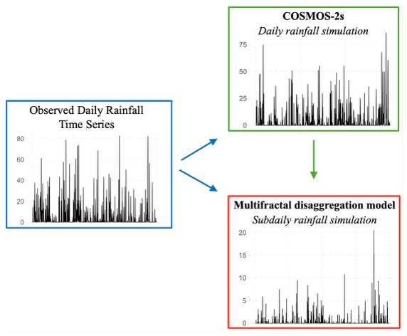
Table 1 Methodological background and specific contributions of Virtual Rain v1.0.

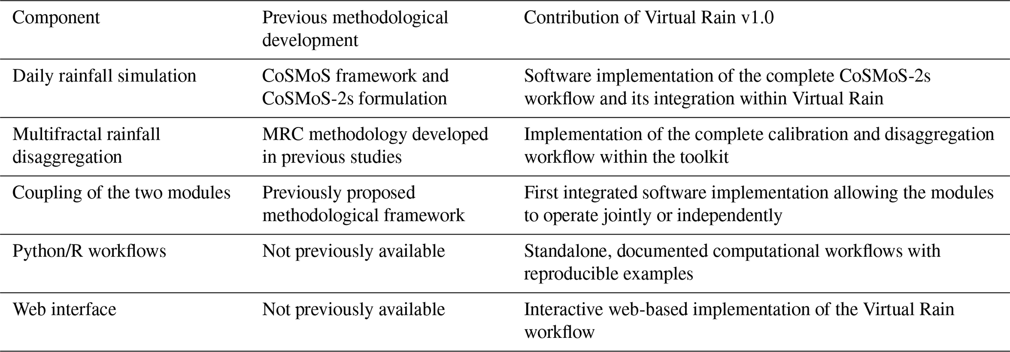
Compared with the previous methodological studies, the novelty of the present contribution lies in the development, implementation, integration, documentation, and verification of the Virtual Rain software framework, rather than in the development of new stochastic rainfall methodologies. Virtual Rain provides the first integrated implementation of the complete CoSMoS-2s workflow (Module 1) and the complete MRC calibration and disaggregation workflow (Module 2) through standalone Python and R routines, complemented by an interactive web-based platform that reproduces the same computational workflow. The specific developments introduced in the present work include the integration of the two previously independent methodological components, their implementation as accessible computational workflows, the development of user interfaces and supporting documentation, and the provision of reproducible examples and implementation-verification procedures. Table 1 summarizes the distinction between previously established methodological developments and the new software and technical contributions introduced by Virtual Rain v1.0.

The proposed software is demonstrated through a real-world case study involving a single rain gauge station. The purpose of the case study is to illustrate the implementation and application of the complete Virtual Rain workflow and to verify the consistency of the software outputs with the expected behavior of the underlying methodologies, rather than to provide a new methodological validation of CoSMoS-2s or the MRC model. Consistent with the Development and technical paper scope, particular attention is therefore given to workflow reproducibility, implementation verification, and consistency among the computational interfaces.

The remainder of the paper is structured as follows. Section 2 presents the underlying methodology. Section 3 describes the Virtual Rain framework and its software implementation. Section 4 presents the case study. Section 5 discusses the main findings, practical implications, and limitations of the proposed implementation. Finally, Sect. 6 concludes the paper, while the Appendix provides an overview of the web-based platform.

2 Methodology in brief

Reliable hydrological modelling, flood risk assessment, and climate variability analyses critically depend on the availability of long-term, high-resolution rainfall records (Grimaldi et al., 2022; Northrop, 2024; Volpi et al., 2024; Fischer et al., 2025).

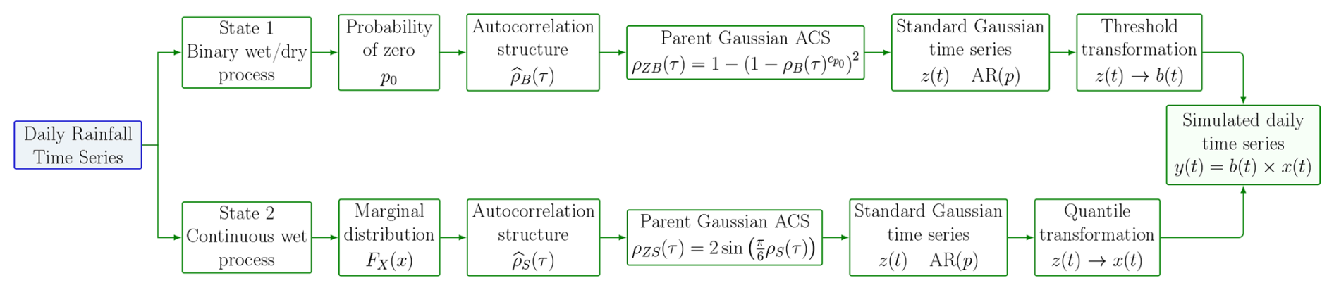
Figure 2 Workflow of Daily Rainfall Simulation Model. Equations details are described in the text.

Figure 3 Workflow of Sub-Daily Rainfall Disaggregation Model. Blue boxes represent the procedure input.

The Virtual Rain framework consists of two modules (Fig. 1): (i) a daily rainfall simulation module based on CoSMoS-2s and (ii) a multifractal temporal disaggregation module based on an MRC model. Depending on data availability and modelling objectives, the two modules can be used either jointly or independently.

The methodological details of the daily simulation and disaggregation procedures are described in Sects. 2.1 and 2.2, respectively.

2.1 Module 1 – daily rainfall simulation model

Daily rainfall time series are simulated using CoSMoS-2s, a two-state intermittent stochastic model (Papalexiou, 2022; Cappelli et al., 2024). In the single-site configuration adopted here, the model is structured around two coupled components: (i) State 1, a binary wet/dry occurrence process and (ii) State 2, a continuous intensity process defined for wet days (Fig. 2).

Since rainfall is usually affected by seasonality, it is necessary to group data into subsets (i.e., $m=\mathrm{1},\mathrm{2},\mathrm{\dots },\mathrm{12}$ seasons), with the aim of modeling rainfall occurrence and intensity within homogeneous samples. The two processes are then modeled separately. In State 1, the observed daily rainfall is transformed into a binary process B(t). For each season, occurrence probabilities p₀ and empirical ACSs (${\widehat{\mathit{\rho }}}_B\left(\mathit{\tau }\right)$) are estimated and subsequently mapped into gaussian correlations through the transformation: ${\mathit{\rho }}_Z\left(\mathit{\tau }\right)=\mathrm{1}-(\mathrm{1}-{\mathit{\rho }}_B(\mathit{\tau }{)}^{c_{p_{\mathrm{0}}}}{)}^{\mathrm{2}}$. Temporal dependence is then reproduced using a gaussian autoregressive (AR) model of order p, and simulated values are converted back into wet/dry states using seasonally varying thresholds. Specifically,

$$\begin{array}{}\text{(1)}& b_m\left(t\right)=\left\{\begin{array}{l}\mathrm{0},z_m\left(t\right)\le z_{p_{\mathrm{0}},m}\left(t\right)\\ \mathrm{1},z_m\left(t\right)>z_{p_{\mathrm{0}},m}\left(t\right)\end{array}\right.\end{array}$$

where $z_{p_{\mathrm{0}},m}={\mathrm{\Phi }}^{-\mathrm{1}}\left(p_{\mathrm{0},m}\right)$ and Φ⁻¹ is the inverse of the cumulative distribution function of the standard normal distribution 𝒩(0,1).

State 2 is devoted to the continuous process X(t) describing the wet-day rainfall amounts. For each season, suitable parametric distributions (e.g., 2- and 3-parameter Gamma, Generalized Gamma, Burr III, Burr XII, and 2- and 3-parameter Weibull distributions) are fitted to non-zero rainfall values, and parametric ACSs are used to model the empirical Spearman ACS S computed from consecutive wet-day sequences.

These correlations are transformed into gaussian equivalents through the parent gaussian ACS ${\mathit{\rho }}_{ZS}\left(\mathit{\tau }\right)=\mathrm{2}\sin \left(\frac{\mathit{\pi }}{\mathrm{6}}{\mathit{\rho }}_S\right(\mathit{\tau }\left)\right)$ and reproduced through an autoregressive model of order p. The simulated gaussian values are then mapped back to rainfall intensities via inverse transformation by applying x(t)=QX(Φ_Z(z(t)) where QX is the quantile function of the fitted rainfall distribution and Φ_Z is the standard gaussian cumulative distribution function.

The final synthetic series is obtained by combining the occurrence and intensity components, allowing the model to reproduce key features such as intermittency, marginal distributions, and temporal persistence (Cappelli et al., 2026a).

2.2 Module 2 – sub-daily rainfall disaggregation model

This module is designed to disaggregate a simulated (by Module 1) or observed daily rainfall time series into high-resolution sub-daily time series using a multifractal random cascade (MRC) model (Cappelli et al., 2025a, b) (Fig. 3). The approach assumes that rainfall intensity evolves as a multiplicative cascade process, in which the mean intensity at each temporal scale is redistributed through random weights with prescribed statistical properties. These weights follow a beta-lognormal distribution. The MRC model is characterized by three parameters: C_β, controlling intermittency and the proportion of dry intervals; C_LN, governing lognormal variability and intensity fluctuations; and D, representing the outer-scale parameter that defines the range of multifractal behavior. Importantly, D represents a scaling parameter of the theoretical multifractal formulation and should not be interpreted as the duration of the rainfall block subsequently disaggregated by the cascade.

The complete mathematical formulation of the MRC model adopted in Virtual Rain, including the beta-lognormal weight distribution, recursive cascade construction, conservation rule, theoretical multifractal IDF formulation, and calibration objective, is provided in Cappelli et al. (2025a, b). The present section summarizes the elements required to understand the role of Module 2 within Virtual Rain, while avoiding duplication of the complete methodological derivation already reported therein. Virtual Rain implements this formulation without introducing modifications to the underlying MRC model; implementation-specific choices and the corresponding input parameters are documented in the software-description section and in the archived software documentation.

Rather than calibrating these parameters using high-resolution rainfall observations, the implemented workflow derives them from IDF relationships, following Cappelli et al. (2025a). IDF curves are typically expressed as $i(d,T)=a\left(T\right)d^{n-\mathrm{1}}$ where i(d,T) is the rainfall intensity associated with duration d with return period T, and n is a scaling exponent constant with $\mathrm{0}<n<\mathrm{1}$, and a(T) is a function independent of d. The parameters C_β, C_LN, and D are jointly estimated through numerical optimization by matching the theoretical multifractal IDF relationships to the target IDF information. Within this calibration, D enters the theoretical formulation through the scale ratio $D/d$ (Cappelli et al., 2025a, b). The theoretical relationship linking the MRC parameters to the IDF scaling properties, together with the objective function used for their calibration, parameter constraints, and optimization procedure, follows the formulation given in Cappelli et al. (2025a, b). By matching theoretical multifractal IDF relationships to empirical IDF curves, it is possible to estimate C_β, C_LN, and D without relying on sub-daily calibration data. The cascade procedure is applied independently to each simulated day, ensuring exact preservation of daily rainfall totals while generating physically consistent sub-daily variability. Once the MRC parameters have been calibrated, the stochastic redistribution within each daily block is governed by C_β and C_LN; therefore, a fitted value of D greater than 24 h does not imply that a multi-day cascade of duration D is explicitly simulated. The cascade recursion and conservation condition are those defined in Cappelli et al. (2025a, b), to which readers are referred for the complete mathematical derivation and definition of all associated variables.

For reproducibility, the specific input variables, parameter units and constraints, preprocessing operations, optimization settings, convergence criteria, and output structure used by the Virtual Rain implementation are reported in Sect. 3 and in the README accompanying the archived software release.

Table 2 Main routines implemented in Virtual Rain.

3 Virtual Rain: a unified toolkit

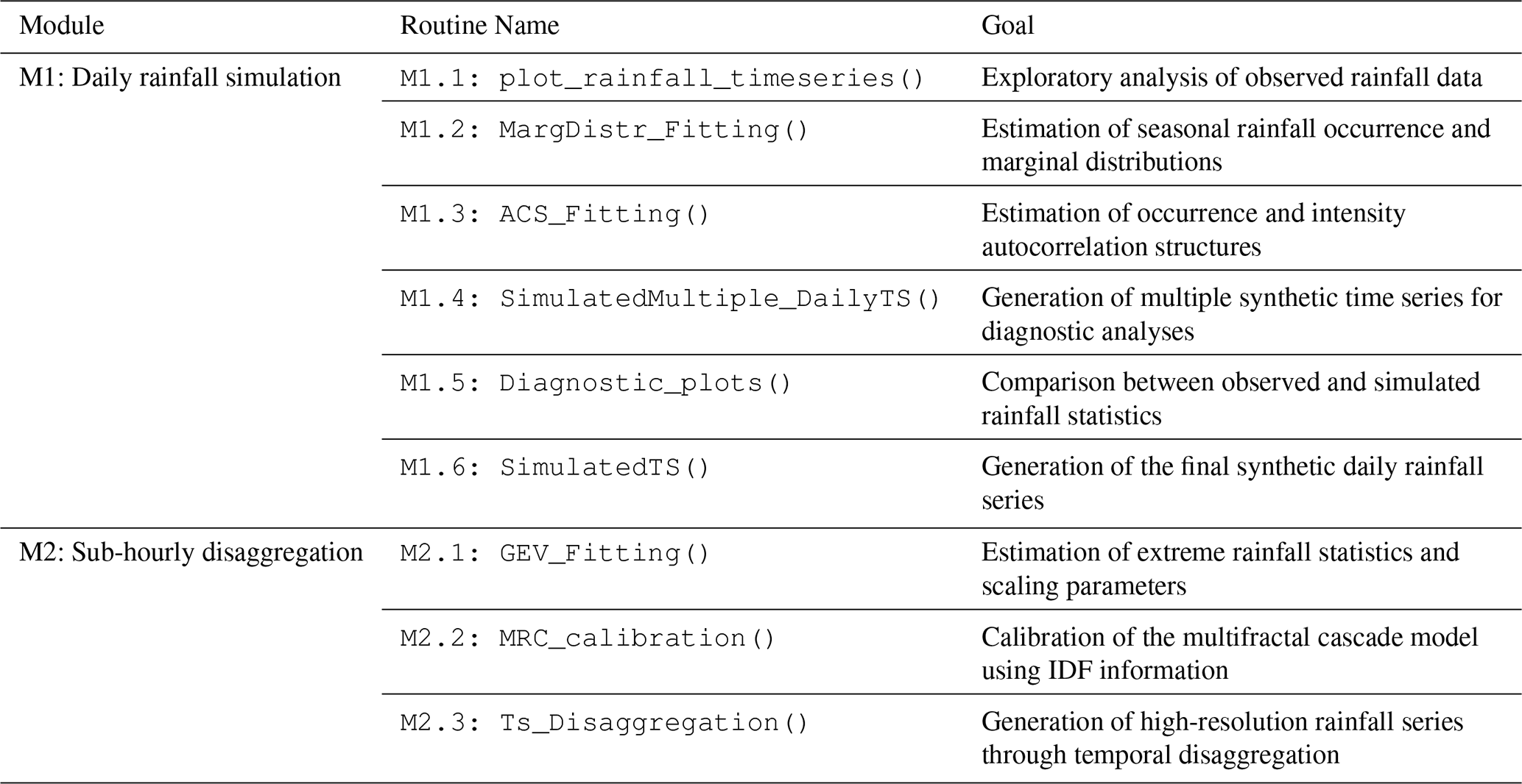
In line with the methodological framework described in Sect. 2, Virtual Rain is organized into two modules: Module 1, dedicated to daily rainfall simulation using CoSMoS-2s, and Module 2, dedicated to temporal disaggregation using the MRC model. Each module consists of a set of routines that guide the user through data analysis, model calibration, simulation, validation, and generation of final outputs.

Table 2 summarizes the main routines implemented in the toolkit and their respective functions.

The following sections describe each routine, including its goal, required inputs, main operations, and outputs.

3.1 Implementation of the daily rainfall simulation module

This module includes six routines designed to guide the user through the complete workflow of stochastic daily rainfall simulation, from exploratory analysis of the observed series to the generation and validation of synthetic rainfall data. The routines allow the user to reproduce key statistical rainfall properties, including marginal distributions, intermittency, seasonality, and temporal dependence, while providing graphical and quantitative tools to support model selection and validation. The routines are described below.

⋆

M1.1:   plot_rainfall_timeseries(data)

Goal: The routine provides a preliminary exploratory analysis of the observed rainfall series and helps the user visually inspect the main rainfall characteristics before model fitting.

Input:

• data: observed daily rainfall time series.

Operations: The function preprocesses the input series and produces three diagnostic plots:

• 1.

  Daily rainfall during the first observation year, useful for visualizing intermittency and wet/dry alternation;

• 2.

  Annual maximum daily rainfall, allowing the user to inspect interannual variability and extreme events;

• 3.

  Monthly seasonal components, highlighting the seasonal rainfall regime and supporting the choice of the seasonal grouping.

Outputs:

• plots of rainfall time series, annual maxima and monthly seasonal components.

⋆

M1.2:   MargDistr_Fitting(data, seasonality_option = (1,2,3,4,6,12), start_month=1)

Goal: The routine identifies the probability distribution that best describes rainfall intensities in each season.

Inputs:

• data: observed daily rainfall time series.

• seasonality_option: number of seasonal groups used to partition the data (e.g., annual = 1, semiannual = 6, quarterly = 3, monthly = 12);

• start_month: starting month of the seasonal partition.

Operations: For each seasonal group, the routine:

• 1.

  estimates the probability of dry days (p₀);

• 2.

  fits seven candidate distributions (2- and 3-parameter Gamma, Generalized Gamma, Burr III, Burr XII, and 2- and 3-parameter Weibull distributions) to non-zero rainfall values:

• 3.

  estimates model parameters through the Nelder–Mead optimization algorithm by minimizing discrepancies between empirical and theoretical exceedance probabilities.

Outputs:

• Estimated parameters for all candidate distributions;

• Diagnostic plots comparing empirical and fitted distributions;

• Summary table containing Relative Mean Absolute Error values (RMAE) estimated on empirical and fitted distributions.

The resulting object (resM1.2) is used as input by the SimulatedMultiple_DailyTS() and SimulatedTS() routines.

⋆

M1.3:   ACS_Fitting(data, lags, seasonality_option = (1,2,3,4,6,12), start_month = 1)

Goal: Estimate the autocorrelation structure of rainfall occurrence and intensity processes.

Inputs:

• data: observed rainfall time series;

• lags: maximum lag considered in the autocorrelation analysis;

• seasonality_option: seasonal grouping window (same of M1.2);

• start_month: starting month of the seasonal partition.

Operations: For each seasonal group and both the binary occurrence process B(t) and the continuous intensity processes X(t), the routine:

• 1.

  computes empirical Spearman autocorrelations;

• 2.

  fits candidate parametric ACSs (Pareto II, Weibull, Burr XII);

• 3.

  estimates model parameters by minimizing the Mean Absolute Error (MAE) between empirical and theoretical ACS values.

The ACS fitting procedure is independent of the marginal distribution selected in Routine M1.2, since it is performed directly on the empirical ACS. Users may subsequently choose whether to use the fitted parametric ACS or the empirical ACS directly during rainfall simulation.

Outputs:

• Estimated ACS parameters;

• Diagnostic plots comparing empirical and fitted ACS for each season and process.

The resulting object (resM1.3) is used as input by the SimulatedMultiple_DailyTS() and SimulatedTS() routines.

⋆

M1.4:   SimulatedMultiple_DailyTS(data, n_simulations, resM1.2, resM1.3, p, seasonality_option, start_month, marg_distr = ('gamma', 'gamma3','ggamma', 'burrIII', 'burrXII', 'weibull', 'weibull3'), acf_distr_BT = ('pare-toII', 'weibull', 'burrXII','empirical'), acf_distr_CT = ('paretoII', 'weibull', 'burrXII','empirical'))

Goal: Generate an ensemble of synthetic rainfall series for model evaluation and uncertainty assessment.

Inputs:

• data: observed rainfall time series;

• n_simulations: number of synthetic time series to generate;

• resM1.2: output from MargDistr_Fitting() routine, including the estimated parameters of all candidate marginal distributions and the observed dry-day frequency (p0);

• resM1.3: output from ACS_Fitting() routine, including the empirical and fitted ACS coefficients;

• p: autoregressive order;

• seasonality_option: number of seasonal groups used in the calibration.

• start_month: starting month of the seasonal partition.

• Marg_distr: selected marginal distribution for rainfall intensities.

• Acf_distr_BT, acf_distr_CT: selected ACS for the binary B(t) and continuous X(t) processes.

Operations: The routine generates multiple synthetic daily rainfall series having the same length as the observed dataset

Outputs:

• Ensemble of synthetic rainfall time series.

The resulting object (resM1.4) is used as input for the Diagnostic_plots() routine.

⋆

M1.5:   Diagnostic_plots(data, resM1.4)

Goal:The routine evaluates the ability of the stochastic model to reproduce the main statistical characteristics of observed rainfall.

Inputs:

• data: observed rainfall time series;

• resM1.4: ensemble of synthetic rainfall series generated by SimulatedMultiple_TS() routine.

Operations: The routine compares observed statistics against simulated distributions using four diagnostic groups:

• 1.

  autocorrelation structure;

• 2.

  seasonal component;

• 3.

  ranked annual maxima;

• 4.

  summary statistics, including dry-day probability (p₀), mean wet-day rainfall (mean), standard deviation (sd), extreme percentiles (P95, P99, P99.9).

Outputs:

• Diagnostic plots comparing observed statistics with the distribution of the simulated ensemble.

⋆

M1.6:   SimulatedTS(data, resM1.2, resM1.3, p, n_years, seasonality_option, start_month, marg_distr, acf_distr_BT = ('paretoII', 'weibull', 'burrXII','empirical'), acf_distr_CT = ('paretoII', 'weibull', 'burrXII','empirical'))

Goal: Generates a synthetic daily rainfall time series using the selected modelling configuration.

Inputs:

• data: observed rainfall time series;

• resM1.2: output from MargDistr_Fitting() routine, including the estimated parameters of all candidate marginal distributions and the observed dry-day frequency (p0);

• resM1.3: output from ACS_Fitting() routines, including the empirical and fitted ACS coefficients;

• p: autoregressive order;

• n_years: desired simulation length

• seasonality_option: number of seasonal groups used in the calibration.

• start_month: starting month of the seasonal partition.

• marg_distr: selected marginal distribution for rainfall intensities.

• acf_distr_BT, acf_distr_CT: selected ACS for the binary B(t) and continuous X(t) processes.

Operations: The routine simulates the wet/dry occurrence process and the wet-day intensity process separately using the calibrated seasonal probabilities, marginal distributions, and autocorrelation structures. The two components are subsequently combined to generate a continuous synthetic daily rainfall series of the specified length.

Outputs:

• Synthetic daily rainfall time series with user-defined duration.

3.2 Implementation of the sub-hourly rainfall disaggregation module

This module includes three routines designed to guide the user through the complete workflow of rainfall temporal disaggregation, from the estimation of extreme rainfall properties to the generation and validation of high-resolution synthetic rainfall series. The routines allow the user to disaggregate daily rainfall while preserving scale-invariant properties and reproducing the imposed IDF scaling exponent through a stochastic MRC approach.

The routines are described below.

⋆

M2.1:   GEV_Fitting(data, starting_day = '2000-01-01', num_of_days_for_truncation = 183, n_par = 0.3)

Goal: Estimate the extreme rainfall statistics and scaling parameters required for MRC calibration.

Inputs:

• data: observed rainfall time series;

• starting_day: starting date of the time series used to construct the temporal index;

• num_of_days_for_truncation: threshold used to exclude incomplete initial or final years;

• n_par: externally imposed scaling exponent representing the slope of the IDF/DDF relationships. This parameter can be estimated from local sub-daily observations or obtained from independent regional IDF/DDF information. In the present case study, n was estimated from the observed sub-daily record and therefore represents a calibration input rather than a model output.

Operations: The routine:

• 1.

  extracts annual maximum rainfall time series;

• 2.

  transforms annual maxima into scaling-based a-IDF coefficients using the imposed scaling exponent n;

• 3.

  fits a GEV distribution to the a-coefficients using three estimation methods: Maximum Likelihood (mle), Probability Weighted Moments (pwm), L-moments (L-mom);

• 4.

  estimates mean annual rainfall intensity;

• 5.

  computes a-coefficients associated with return periods ranging from 2 to 999 years using both: parametric approaches (GEV-based) and empirical approaches. These a-coefficients are subsequently used to constrain the matching between the target and simulated IDF curves during the MRC calibration procedure. The interval 2–999 years represents the admissible range implemented in the software, where 999 years is simply adopted as the maximum allowable return period to provide flexibility to the user. In practical applications, however, the selected return periods should be commensurate with the length of the available annual maximum series, since estimates associated with increasingly large return periods become progressively more uncertain.

Outputs:

• GEV parameter estimates for the three fitting methods;

• a-coefficients associated with different return periods;

• Annual maxima time series;

• Diagnostic plots including: (1) daily rainfall during the first year, (2) annual maximum daily rainfall over the observation period, (3) Gumbel plots comparing empirical and fitted distributions.

The resulting object (resM2.1) is used as input for the MRC_calibration() routine.

⋆

M2.2:   MRC_calibration(resM2.1, lower_bounds = c(Cb_Lb, Cln_Lb, D_Lb), upper_bounds = c(Cb_Ub, Cln_Ub, D_Ub), Return_periods = c(2, 4, 6, 8, 10), n_par, method = c('mle', 'pwm', 'L-mom', 'empirical'), Num_Iterations, a_Rp = NULL)

Goal: Calibrate the MRC model parameters required to reproduce the imposed rainfall scaling properties and IDF relationships.

Inputs:

• resM2.1: output from GEV_Fitting() routine, including the scaling-based a-coefficients, the estimated mean annual rainfall intensity, and the observed rainfall time series.

• lower_bounds, upper_bounds: admissible parameter ranges for calibration. By default, the routine adopts the following literature-based bounds: $C_{\mathit{\beta }}\in [\mathrm{0.1},\mathrm{0.7}];C_{\text{LN}}\in [\mathrm{0.01},\mathrm{0.1}];D\in [\mathrm{24},\mathrm{2400}]$.

• Return_periods: return periods used to constrain the calibration through the matching of target and simulated IDF curves.

• n_par: externally imposed scaling exponent representing the slope of the IDF/DDF relationships. This parameter can be estimated from local sub-daily observations or obtained from independent regional IDF/DDF information. In the present case study, n was estimated from the observed sub-daily record and therefore represents a calibration input rather than a model output.

• method: method used to estimate the a-coefficients (mle, pwm, L-mom, or empirical).

• Num_Iterations: maximum number of optimization iterations;

• a_Rp (optional): user-defined a-coefficients. When provided, these coefficients replace those estimated by GEV_Fitting(), allowing users to directly incorporate externally derived IDF information (e.g., regional IDF curves, published studies, or expert knowledge). This option extends the applicability of Virtual Rain to ungauged or data-sparse regions and supports scenario analyses based on modified rainfall scaling characteristics, such as those associated with climate change.

Operations: The routine estimates the MRC parameters (C_β, C_LN, D) through numerical optimization. The optimal parameter set is defined by minimizing discrepancies between theoretical and empirical IDF curves associated with the imposed scaling exponent nand the selected a-coefficients for the chosen return periods. By default, the target a-coefficients are obtained from GEV_Fitting(), although users may alternatively provide externally derived coefficients through the optional a_Rp argument. The calibration procedure, including the definition of the objective function, the weighting strategy adopted for the IDF curves, and the numerical optimization approach, is described in detail in Sect. 2.3 of Cappelli et al. (2025b). Because the a-coefficients are estimated by fitting a GEV distribution to the available annual maxima, the associated uncertainty depends on both the record length and the extrapolation to the selected return periods.

Outputs:

• Calibrated MRC parameters (C_β, C_LN, D);

• Objective function value at convergence;

• Diagnostic plots comparing empirical and theoretical IDF curves.

The resulting object (resM2.2) is used as input for the Ts_Disaggregation() routine.

⋆

M2.3:   Ts_Disaggregation(resM2.2, ending_time_resolution = 15, N_simulations = NULL, preserve_rainfall_volume = c('Yes', 'No'), seed = c('Yes', 'No'))

Goal: Generate high-resolution rainfall series through temporal disaggregation of daily rainfall using the calibrated MRC model.

Inputs:

• resM2.2: output from MRC_calibration() routine, including the calibrated values of the MRC parameters (C_β, C_ln, D), which are used to perform the disaggregation;

• ending_time_resolution: target temporal resolution (1–60 min).

• N_simulations: number of disaggregated time series to generate.

• preserve_rainfall_volume: option to preserve daily rainfall totals. Preserving daily totals is the default and recommended setting for standard rainfall disaggregation, as it ensures consistency between daily and sub-daily rainfall amounts.

• seed: option to initialize the random number generator for reproducibility.

Operations: The routine applies the calibrated MRC model to disaggregate daily rainfall into sub-daily intervals. The cascade is applied only to wet days, recursively redistributing daily rainfall volumes while preserving the prescribed scaling properties and, optionally, the original daily totals. One or more stochastic realizations can be generated at the selected temporal resolution.

Outputs:

• Disaggregated rainfall time series;

• Plots of the observed daily time series and the corresponding disaggregated one for the first simulated year;

• Summary tables reporting key rainfall statistics, ACS coefficients, annual maxima over multiple durations, and IDF-related indicators for each simulation.

The resulting outputs allow users to visually inspect the generated series and evaluate whether the simulated scaling and IDF characteristics are consistent with the calibration targets, namely the prescribed scaling exponent nand the prescribed a-coefficients for the considered return periods.

This module includes six routines designed to guide the user through the complete workflow of stochastic daily rainfall simulation, from exploratory analysis of the observed series to the generation and validation of synthetic rainfall data. The routines allow the user to reproduce key statistical rainfall properties, including marginal distributions, intermittency, seasonality, and temporal dependence, while providing graphical and quantitative tools to support model selection and validation. The routines are described below.

3.3 Interactive digital platform

The routines described in the previous sections are mainly intended for advanced users with programming experience in Python and R. To make the proposed toolkit accessible to a wider scientific and technical audience, an interactive web-based platform, Virtual Rain (https://www.hydrolab.unitus.it/virtualrain, last access: 29 September 2026), has been designed and developed. Its main interfaces are reported in the Appendix.

The web platform follows the same logical structure as the routines presented above, guiding users' step by step through the modelling workflow, from input data processing to model calibration, simulation, and diagnostic evaluation. The main model parameters introduced in the methodological framework can be modified directly by the user, providing a flexible environment for both operational applications and methodological exploration.

Importantly, the standalone Python and R routines and the Virtual Rain web platform implement the same methodological formulations, computational workflow, and model parameterization. Because both daily rainfall generation and sub-daily disaggregation involve stochastic simulation, individual synthetic realizations are not expected to be numerically identical across the different software environments, even when the same input data and model parameters are used. Cross-interface consistency should therefore be interpreted in terms of equivalence of the implemented algorithms and parameterization and, for stochastic outputs, reproduction of the same target statistical properties rather than point-by-point equality of the generated series. These properties include rainfall intermittency, marginal distributions, temporal dependence, preservation of daily rainfall totals during disaggregation, and the statistical characteristics of sub-daily rainfall prescribed by the MRC model. For deterministic components of the workflow, consistency can instead be assessed through direct comparison of the corresponding parameters and intermediate computational outputs.

By combining computational routines with an intuitive graphical interface, Virtual Rain reduces the technical barrier associated with coding while preserving the flexibility of the proposed modelling framework. The web platform therefore provides an alternative interface to the same computational framework rather than a separate modelling implementation. It supports not only practical model implementation, but also a clearer understanding of the underlying stochastic processes, parameter choices, and diagnostic outputs. Overall, Virtual Rain represents a comprehensive tool that bridges methodological flexibility and practical usability, making the proposed framework suitable for research applications, advanced professional analyses, and educational purposes.

4 Case study: Arno rain

To illustrate the effectiveness and flexibility of the proposed framework, we present a case study based on a daily rainfall time series (Station code TOS01004779) selected from a dataset of more than 70 rain gauges distributed across the Arno River Basin. The Arno is one of the longest rivers in Italy, and it is the main river system in Tuscany, Central Italy. The dataset spans the period from 1 January 2001 to 31 December 2020 (Cappelli et al. 2026b). The dataset comprises 70 rain gauges located across the Arno River Basin, all providing continuous and contemporaneous 15 min rainfall observations over the common 20-year period (2001–2020) and satisfying the quality-control criteria adopted in Cappelli et al. (2025b, 2026b). Consequently, the 20-year period represents the longest common observation window available across the entire monitoring network. Further details on the dataset preparation and quality-control procedures are provided in Cappelli et al. (2025b, 2026b).

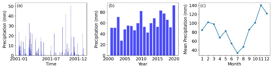
Figure 4 Overview of the input observed daily time series: (a) daily rainfall for the first year, (b) annual maximum daily rainfall, and (c) monthly mean seasonal component.

The 2001–2020 observational record is used both for model calibration and for the subsequent diagnostic comparison with the simulated series. Accordingly, the comparison between observed and simulated statistics should be interpreted as a calibration diagnostic aimed at verifying the ability of the calibrated stochastic model to reproduce the target statistical characteristics and at demonstrating the correct implementation of the Virtual Rain workflow, rather than as an assessment of predictive performance on an independent validation dataset.

The proposed modelling framework and its underlying procedures have already been extensively tested in previous studies on several rainfall datasets and climatic conditions, yielding satisfactory results in terms of reproducing rainfall intermittency, temporal dependence, scaling properties, and extreme-event statistics (Cappelli et al., 2024, 2025b, 2026a, c). Accordingly, the objective of the present case study is not to provide a new methodological validation of CoSMoS-2s or the MRC model, but to demonstrate the practical implementation of the complete Virtual Rain workflow and verify to assess whether the integrated software implementation reproduces the statistical behaviour expected from the underlying methodologies.

4.1 Results of the daily rainfall simulation module

As described in Sect. 3.1, The plot_rainfall_timeseries() routine of the Daily Rainfall Simulation Module provides an overview of the observed daily time series (Fig. 4).

It produces three plots: daily rainfall for the first year, annual maximum rainfall over the full observation period, and monthly mean seasonal component. The seasonal component (Fig. 4c) is intended to provide users with a visual summary of the annual rainfall cycle to support the selection of an appropriate seasonal partition. It assists users in choosing both the number of seasonal groups and the starting month according to the characteristics of the rainfall regime. In the present case study, three seasonal groups starting in April were adopted as a compromise between representing the main seasonal variability and ensuring a sufficient sample size for robust estimation of the marginal distributions and autocorrelation structure. The seasonal grouping is therefore user-defined and is not selected automatically by the software.

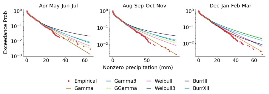
Figure 5 Calibration results of the seven candidate marginal distributions fitted on non-zero rainfall values.

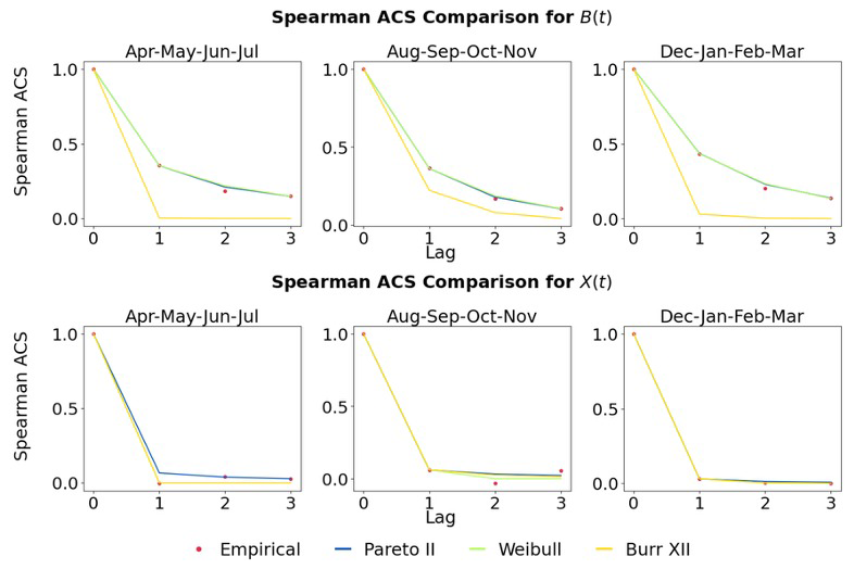
Figure 6 Comparison between empirical and fitted parametric ACSs for the B(t) and X(t) processes across the seasonal groups. The fitted curves are obtained by minimizing the Mean Absolute Error between empirical and theoretical Spearman ACSs.

Table 3 Relative Mean Absolute Error (RMAE) associated with the candidate marginal distributions for each seasonal group. Lower RMAE values indicate better agreement between empirical and theoretical exceedance probabilities, particularly for the upper tail of the rainfall distribution (values above the 50th percentile).

Non-zero rainfall values are modeled using seven candidate distributions (Gamma, three-parameter Gamma, Generalized Gamma, Weibull, three-parameter Weibull, Burr III, and Burr XII). The parameters of each candidate distribution are estimated by minimizing the distance between empirical and theoretical exceedance probabilities using the Nelder–Mead optimization algorithm. Model performance is evaluated using the RMAE computed over the upper tail (values above the 50th percentile), as lower values are generally well reproduced by all candidate distributions. The objective of the procedure is to identify a single marginal distribution family to be adopted consistently across all seasons, while estimating its parameters independently for each season. When the same distribution provides the best fit for every season, it is selected directly. Otherwise, the routine returns the estimated parameters for all candidate distributions together with a summary table of seasonal RMAE values, allowing the user to select the most appropriate common marginal distribution based on its overall performance across seasons. The calibration results obtained using MargDistr_Fitting() routine (Fig. 5 and Table 3) indicate that the Gamma distribution provides the best overall performance.

The autocorrelation structure is then modeled using the ACS_Fitting() routine, which estimates the Spearman ACS accounting for seasonality and distinguishing between B(t) and X(t) processes.

After selecting the maximum lag, parametric ACS models (Pareto II, Weibull, and Burr XII) are fitted separately for the two processes B(t) and X(t) by minimizing the MAE between empirical and parametric ACSs. Figure 6 compares the empirical and fitted ACSs, providing a visual assessment of the adequacy of the candidate models. For the binary process, both the Weibull and Pareto II ACS provide a satisfactory representation of the empirical Spearman ACS. Conversely, the Burr XII model exhibits a less accurate fit for the third seasonal group because the empirical ACS decays more slowly than can be reproduced by the fitted Burr XII function, highlighting the limitations of this parametric form for representing the observed persistence pattern. For the continuous process, all three candidate ACSs accurately reproduce the empirical Spearman ACS. In this case study application p=3 and the empirical ACS are adopted.

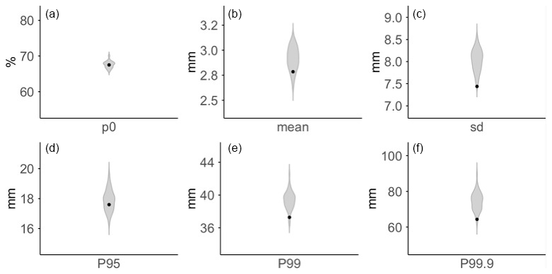
Figure 7 Comparison between observed (black dots) and 50 simulated (gray violin plots) summary statistics of non-zero rainfall: (a) probability of zero, (b) mean, (c) standard deviation, (d) 95th percentile, (e) 99th percentile, and (f) 99.9th percentile.

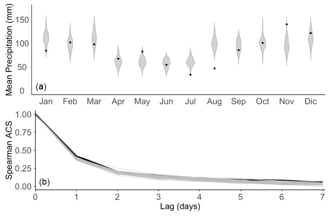
Figure 8 Comparison of: (a) seasonal components between observed (black dots) and 50 simulated (gray violin plots) series (upper panel); (b) Spearman autocorrelation functions between observed (black line) and 50 simulated series (gray lines) (bottom panel).

Based on the results of the previous calibration steps, the selected marginal distributions and ACS models are subsequently used within the SimulatedMultiple_DailyTS() routine to generate an ensemble of 50 synthetic daily rainfall time series having the same length as the observed record. The use of multiple realizations is an integral part of the Module 1 workflow because the user must evaluate a model configuration resulting from several choices, including the seasonal grouping, marginal distribution, dry-day probability, ACS representation, and AR order. The ensemble therefore provides a robust basis for assessing the stability of the selected CoSMoS-2s configuration and the variability associated with the stochastic simulation process. The resulting ensemble is then provided as input to the Diagnostic_plots() routine, which compares observed and simulated rainfall characteristics, including autocorrelation structure, seasonality, dry-day probability (p0), mean and standard deviation of wet-day rainfall, and extreme percentiles. These comparisons are intended to verify that the implemented stochastic simulation workflow correctly reproduces the statistical characteristics prescribed during calibration. The results (Fig. 7) show that the model successfully reproduces the main statistical properties of the observed data, including dry frequency and central distribution characteristics, with a slight overestimation in the upper tail. A slight overestimation is observed in the upper tail, which reflects the combined effects of the stochastic nature of the rainfall generator and the limited amount of information available for calibrating the marginal distribution, rather than a systematic model bias. In the present case study, the daily rainfall record spans approximately 20 years and contains nearly 70 % dry days, resulting in a relatively small sample of non-zero rainfall events for estimating the upper-tail behaviour. Because the synthetic daily rainfall series generated by Module 1 is subsequently used as input to Module 2, uncertainty in the representation of the daily upper tail may propagate into the estimation of the a-coefficients and, consequently, into the calibration and outputs of the MRC disaggregation model. Nevertheless, the objective of the present case study is to demonstrate the complete Virtual Rain workflow rather than to isolate the performance of the MRC methodology. Module 2 can also be applied directly to observed daily rainfall series whenever reliable daily observations are available, as described in the Introduction. This application, together with the corresponding assessment of extreme-value reproduction, is presented in Cappelli et al. (2026b). Figure 8 compares the seasonal cycle and the Spearman ACS of the observed and simulated rainfall series. Overall, the model satisfactorily reproduces both the seasonal variability and the temporal dependence across lags, although minor discrepancies are observed for some individual months. These discrepancies are an expected consequence of the adopted user-defined seasonal partition, in which three consecutive months are grouped to increase the amount of data available for estimating the marginal distributions and autocorrelation structure. This choice represents a deliberate trade-off between faithfully reproducing month-to-month variability and obtaining robust parameter estimates from relatively short rainfall records. Although a finer seasonal parameterization (e.g., 12 monthly groups) could improve the representation of the seasonal cycle, it would substantially increase the number of parameters to estimate, reduce the sample size available for each calibration period, and increase the computational cost. In the present case study, the empirical ACS was selected during the ACS_fitting() routine because it provided the most faithful representation of the observed autocorrelation structure. Consequently, the agreement observed over the first p=3 lags is expected, as these lags directly reflect the empirical dependence structure adopted during model configuration, and should therefore not be interpreted as an independent validation of the model's ability to reproduce temporal dependence. Instead, the behaviour at longer lags provides a more informative diagnostic of the implemented stochastic model, demonstrating its ability to propagate temporal dependence beyond the range explicitly used during calibration. The observed discrepancies are an expected consequence of the adopted seasonal parameterization, in which three consecutive months are grouped to increase the amount of data available for estimating the marginal distributions and autocorrelation structure. This configuration represents a deliberate trade-off between faithfully reproducing month-to-month variability and obtaining robust parameter estimates from relatively short rainfall records. Accordingly, a modest reduction in the accuracy of the monthly seasonal cycle is accepted in exchange for improved robustness and stability of the statistical model, ultimately enhancing the reliability of the simulated daily rainfall series.

Figure 9 presents the comparison of ranked annual maxima at different durations. The observed values generally fall within the variability range of the simulated extremes, indicating that the implemented workflow reproduces the prescribed multi-day extreme-rainfall behaviour.

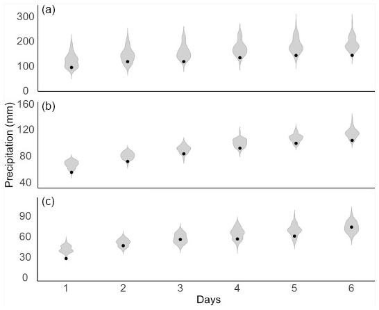
Figure 9 Comparison of (a) highest, (b) median, and (c) lowest ranked annual maxima between observed (black dots) and 50 simulated series (gray violin plots).

Overall, Figs. 7–9 provide a verification of the software implementation by demonstrating that the calibrated stochastic simulation workflow reproduces the target statistical characteristics of the observed rainfall process. The methodological validation of the underlying CoSMoS-2s framework has already been presented in Papalexiou (2022), Cappelli et al. (2026a), Cappelli and Grimaldi (2026).

If the model performance is deemed satisfactory, the user can proceed with the final simulation using the SimulatedTS() routine, specifying the desired length. The generated daily rainfall time series can then be downloaded or directly used as input for Module 2 for temporal disaggregation.

4.2 Results of the sub-hourly rainfall disaggregation module

In contrast to Module 1, the purpose of Module 2 in the present manuscript is not to compare alternative model configurations or to quantify the statistical variability of the MRC methodology through a new ensemble experiment. Once the daily rainfall series, the imposed scaling exponent, and the calibrated MRC parameter set are available, Module 2 applies the established stochastic disaggregation procedure. The case study therefore illustrates a single application of the calibrated MRC workflow, whereas extensive ensemble-based analyses and methodological validation of the MRC model have already been presented in Cappelli et al. (2025a, b).

Besides the daily rainfall series, Module 2 requires the scaling exponent n, representing the slope of the IDF relationship. This parameter is an imposed input of the GEV_Fitting() routine and can either be estimated from available sub-daily rainfall observations or obtained from external sources, such as regional IDF relationships. In the present case study, the imposed value n=0.251 was estimated from the observed 15 min rainfall time series. Specifically, precipitation was aggregated at durations of 1, 3, 6, 12, and 24 h, annual maximum rainfall depths were extracted for each duration, and the resulting DDF relationships were linearized in logarithmic coordinates. The common slope was then estimated by least squares while imposing parallelism among the linearized curves. The resulting value n=0.251 was used, together with the synthetic daily rainfall series generated by Module 1, to calibrate the MRC disaggregation model. Consequently, n should be regarded as an imposed calibration input rather than as a model output.

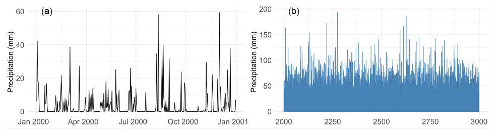
Figure 10 (a) First year of the simulated daily rainfall time series; (b) annual maximum of the simulated daily time series.

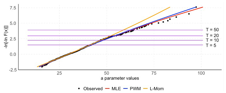
Figure 11 Gumbel plot comparing empirical and theoretical a-coefficients obtained from the fitted GEV distributions using Maximum Likelihood (MLE), Probability Weighted Moments (PWM), and L-moments (L-mom).

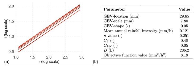
Figure 12 MRC model calibration: (a) comparison between empirical (red line) and theoretical (black line) IDF curves; (b) estimated calibration inputs and calibrated model parameters.

Figures 10 and 11 present the outputs of GEV_Fitting() routine. Figure 10 provides a general overview of the rainfall dataset, including first year of the simulated daily rainfall series (Fig. 10a) and the annual maxima extracted from the entire simulated time series (Fig. 10b). These annual maxima, together with the imposed scaling exponent n, are subsequently used to estimate the scaling-based a-coefficients required for the calibration of the MRC model. Although the routine does not impose a minimum number of annual maxima, longer records generally provide more robust GEV parameter estimates and, consequently, more reliable a-coefficients, particularly for high return periods. Figure 11 shows the Gumbel plot that compares the performance of the alternative GEV fitting methods. The plot supports the selection of the most appropriate method for estimating the a-coefficients used in the MRC calibration. Both mle and pwm provide a good fit to the empirical data.

The MRC_calibration() routine is then used to calibrate the MRC model. In this study, return periods of 10, 20, 50, 100, and 200 years are considered, and the mle method is selected. Figure 12 presents the calibration results. Figure 12a compares the empirical and theoretical IDF curves obtained after calibration, while Fig. 12b reports the corresponding parameter estimates, including the GEV parameters, the calibrated MRC parameters (C_β, C_LN, and D), the mean annual rainfall intensity, and the value of the objective function (8.19 mm² h⁻² for the present case study). The close agreement between the empirical and theoretical IDF curves indicates that the calibrated parameter set reproduces the target IDF relationships prescribed during calibration over the selected range of return periods. The reported objective-function value should be interpreted solely as a case-specific calibration diagnostic and not as a universal indicator of calibration quality. Furthermore, the reliability of the estimated IDF relationships depends on the uncertainty associated with fitting the GEV distribution to the available annual-maximum series, particularly for long return periods. A detailed description of the calibration procedure and objective function is provided in Sect. 2.3 of Cappelli et al. (2025b).

Figure 13 Disaggregated rainfall time series at 15 min resolution (first year).

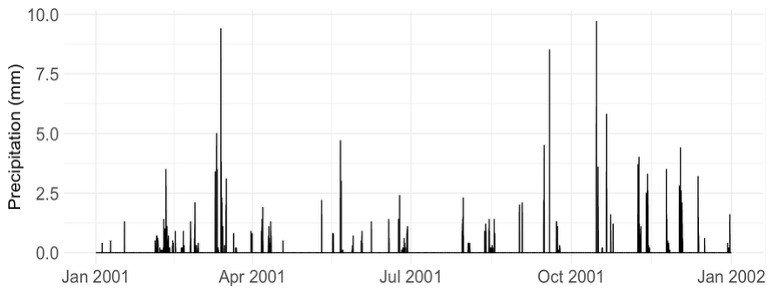
Once the calibration parameters have been estimated, they are used as input to the Ts_Disaggregation() routine, which implements the MRC disaggregation procedure. For illustrative purposes, the simulated daily rainfall time series is disaggregated to a 15 min temporal resolution, generating a single stochastic realization. Figure 13 shows the resulting 15 min rainfall series for the first simulated year.

Finally, a comprehensive summary of the disaggregation results is provided in Table 4. The observed 15 min rainfall series serves two distinct purposes in the present case study: (i) it is used to estimate the target scaling exponent n, which is subsequently imposed as an input to the MRC calibration procedure, and (ii) it provides the benchmark for the diagnostic comparison with the disaggregated rainfall series. The MRC parameters (C_β, C_LN, and D) is performed independently through the MRC calibration procedure using the synthetic daily rainfall series generated by Module 1 together with the imposed value of n. Therefore, the present application represents the data-rich pathway available in Virtual Rain, in which local sub-daily observations are available to estimate n. When such observations are unavailable, the software also allows n to be supplied from independent external information, such as regional IDF/DDF relationships; however, this data-sparse pathway is a software capability and is not explicitly evaluated in the present case study. The subsequent comparison between the observed and disaggregated rainfall series is intended as a diagnostic assessment of the implemented workflow rather than as an independent validation of the MRC methodology.

Table 4 Diagnostic comparison of summary statistics, ACS coefficients, accumulated maxima, and IDF parameters for the observed 20-year rainfall series at 15 min resolution and a 1000-year synthetic rainfall realization generated by the MRC disaggregation model. Owing to the different record lengths, sample-dependent extreme statistics should not be interpreted as directly comparable estimates.

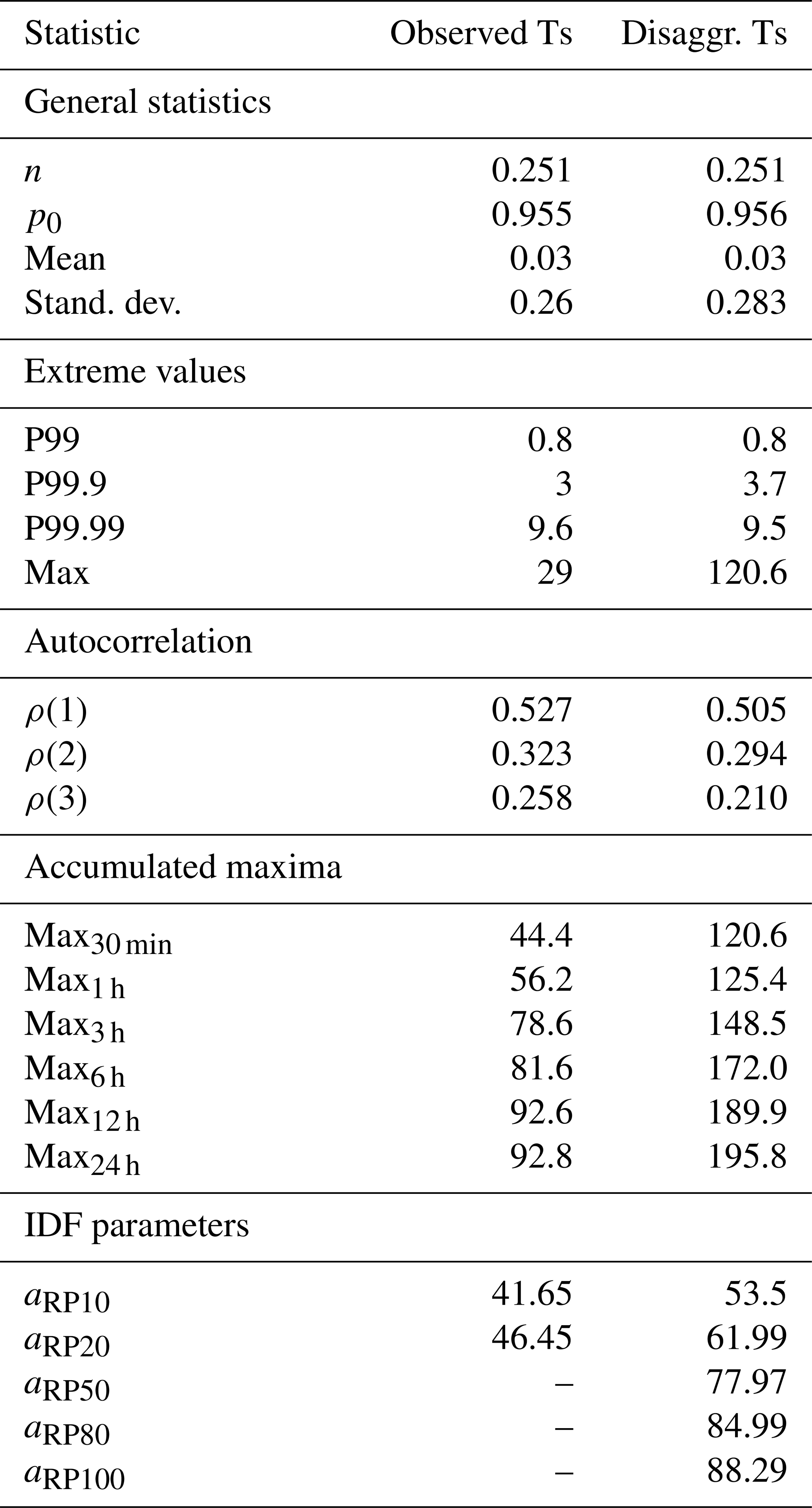
In particular, the scaling exponent n, dry frequency (p0), mean rainfall, and the central and upper portions of the rainfall distribution (e.g., P99 and P99.99) are reproduced with good accuracy. The close agreement between the imposed and simulated scaling exponent demonstrates that the calibration procedure successfully reproduces the prescribed scaling behavior. This result should be interpreted as verification of the correct implementation of the calibration workflow rather than as an independent assessment of the predictive capability of the MRC model. The autocorrelation structure is also satisfactorily preserved, although a slight underestimation of the first autocorrelation coefficients can be observed. Table 4 compares the observed 20-year rainfall series at 15 min resolution with a single 1000-year synthetic realization. Consequently, sample-dependent quantities, particularly absolute maxima and very high empirical percentiles, are not directly comparable between the two records because their sampling variability depends strongly on record length. A matched-length ensemble would provide a more appropriate framework for quantifying the distribution of these diagnostics and the associated Monte Carlo uncertainty. Such an ensemble-based assessment is not included in the present software-oriented study because it requires a substantially larger computational effort and would duplicate the extensive diagnostic analysis of the MRC methodology already presented in Cappelli et al. (2025a, Appendix, Case Study 3), to which interested readers are referred.

As expected, larger differences emerge when considering extreme rainfall properties. These differences should not be attributed exclusively to model performance, because they may arise from both the different record lengths and stochastic variability. In the present workflow, they may also reflect the uncertainty propagated from the synthetic daily rainfall series generated by Module 1, which constitutes the input to the MRC calibration procedure. Therefore, the current case study does not allow the effects of record length and stochastic rainfall generation to be disentangled. The disaggregated time series exhibits higher maximum rainfall accumulations across all aggregation durations, and the empirically estimated a-coefficients are generally larger than those derived from the observed record. Nevertheless, the key calibration targets are reproduced remarkably well. Both the dry-frequency (p0) and the scaling exponent (n)—the latter being the only parameter directly used to calibrate the MRC model—are identical to those observed, confirming the ability of the two modules to preserve rainfall intermittency and scaling properties while remaining consistent with the target IDF relationships. A more extensive assessment based on multiple stochastic realizations and matched record lengths, including the variability of the resulting rainfall statistics, is available in Cappelli et al. (2025a, Appendix, Case Study 3) and is not repeated here. The application of the MRC model directly to observed daily rainfall series, thereby isolating the performance of the disaggregation methodology from the uncertainty introduced by Module 1, is presented and discussed in Cappelli et al. (2026b).

Overall, the results confirm that the calibrated MRC model provides a statistically consistent representation of sub-daily rainfall variability while preserving the prescribed scaling behavior and extreme-value characteristics. Within the context of this software paper, these results demonstrate the correct implementation of the integrated Module 1–Module 2 workflow rather than providing a new methodological validation of the MRC model. Accordingly, Table 4 should be interpreted as a diagnostic illustration of the implemented workflow, while the more computationally intensive ensemble-based evaluation of stochastic uncertainty and record-length effects is documented in the previous methodological study.

5 Discussion

The primary objective of Virtual Rain is not to introduce new stochastic rainfall methodologies, but to provide an operational and reproducible implementation of previously validated approaches within a unified software environment. Accordingly, the case study presented here should be interpreted primarily as a calibration, diagnostic, and software-verification exercise rather than as an independent validation of the underlying CoSMoS-2s and MRC methodologies. The same observational information used for model configuration and calibration is also used for the subsequent diagnostic assessment. The comparison between observed and simulated statistics is therefore intended to verify whether the implemented workflow reproduces the statistical characteristics prescribed during calibration, rather than to assess predictive performance on an independent validation dataset. Broader methodological evaluations of the underlying rainfall-generation and disaggregation approaches are reported in the corresponding previous studies.

An important outcome of this work is that several methodological choices, which are often only implicitly described in previous studies, become explicit user decisions within the software. Consequently, Virtual Rain translates the theoretical flexibility of the underlying models into a structured operational workflow. The user must specify several key configuration elements, including (i) the seasonal partition, (ii) the marginal distribution of non-zero rainfall, (iii) the representation of the autocorrelation structure, (iv) the AR model order, (v) the imposed scaling exponent n, (vi) the return periods adopted during MRC calibration, and (vii) the length of the rainfall time series. These choices inevitably involve trade-offs between statistical accuracy, robustness of parameter estimation, computational efficiency, and data availability.

The seasonal partition represents one of the most influential configuration choices. Increasing the number of seasonal groups generally improves the representation of the annual rainfall cycle but simultaneously reduces the amount of data available for estimating the marginal distributions and autocorrelation structure within each season. Conversely, grouping several consecutive months provides more robust parameter estimates, particularly when relatively short rainfall records are available, at the expense of a less detailed representation of month-to-month variability. Transitions between independently calibrated seasons may also introduce discontinuities in model parameters or dependence properties at seasonal boundaries. Virtual Rain therefore provides diagnostic information to support the user in selecting a seasonal structure appropriate to the available record and application rather than assuming that a single partition is universally optimal.

A similar compromise characterizes the selection of the marginal distribution. The software estimates several candidate distributions independently for each season while encouraging the adoption of a single distributional family throughout the year whenever possible. Although different distributions may locally provide the best statistical fit, adopting a common distribution improves consistency, reproducibility, and interpretability of the resulting stochastic model while limiting unnecessary model complexity. The selected distribution and its fitted parameters remain subject to sampling uncertainty, particularly when seasonal stratification leaves relatively few wet observations. Consequently, differences among similarly performing candidate distributions should not necessarily be interpreted as evidence of a uniquely identifiable marginal model.

The representation of temporal dependence also reflects the balance between flexibility and operational simplicity. In the present application, the empirical ACS structure was adopted because it provided the closest agreement with the observed rainfall series without introducing additional calibration parameters. Virtual Rain nevertheless allows users to employ a parametric ACS whenever a smoother analytical representation is preferred. Similarly, the autoregressive order should not be interpreted as a uniquely identifiable parameter but rather as a practical modelling choice that controls the persistence reproduced by the stochastic generator. Diagnostic comparisons at lags beyond those explicitly included in the autoregressive formulation provide useful information on the ability of the calibrated model to propagate temporal dependence. The MRC disaggregation module follows the same general philosophy. The scaling exponent n is treated as an imposed calibration input and may, in principle, be estimated from local sub-daily observations or obtained from external information such as regional IDF/DDF relationships. In the present case study, however, n=0.251 was estimated from the available 15 min observations. The application presented here therefore represents the data-rich pathway and should not be interpreted as an empirical demonstration of calibration in the complete absence of local sub-daily observations. The possibility of supplying independently derived regional scaling information represents a capability of the software that remains to be evaluated explicitly in data-sparse applications.

The interpretation of the MRC outer-scale parameter D also deserves clarification. The parameter D is jointly estimated with C_β and C_LN during the numerical optimization of the theoretical multifractal IDF relationships and enters the calibration through the scale ratio $D/d$, where d denotes rainfall duration. It therefore represents the outer scale of the calibrated multifractal scaling regime rather than the duration of the rainfall block explicitly disaggregated by the cascade. In the analyzed case study, the fitted value D = 286.2 h consequently does not imply that a continuous 286.2 h cascade is simulated. Following calibration, individual daily rainfall amounts are independently disaggregated using the calibrated cascade parameters while preserving their daily totals. The theoretical interpretation and sensitivity of D are discussed more extensively in the original methodological formulation (Cappelli et al., 2025a).

The integrated use of Modules 1 and 2 introduces an additional source of uncertainty that is important when interpreting the final high-resolution rainfall series. Module 2 receives the synthetic daily rainfall generated by Module 1; consequently, departures generated during daily rainfall simulation may propagate into the subsequent disaggregation stage. Virtual Rain also allows Module 2 to be applied directly to observed daily rainfall, thereby avoiding this specific source of propagated uncertainty when reliable daily observations are available. The present integrated case study does not formally partition the total error into contributions from daily rainfall generation, MRC calibration, and stochastic cascade variability. Application of the MRC model directly to observed daily rainfall, which allows the disaggregation component to be examined separately, is presented in the corresponding methodological study.

Parameter uncertainty represents another limitation of the current implementation. Marginal, dependence, extreme-value, and cascade parameters are represented through point estimates in the operational workflow, and uncertainty in these estimates is not currently propagated through the complete Module 1–Module 2 chain. Moreover, combinations of MRC parameters may provide similarly performing solutions to the numerical calibration problem, making parameter identifiability an aspect that should be considered when interpreting individual fitted values. The current implementation should therefore be regarded as providing an operational calibrated solution rather than a complete probabilistic characterization of parameter uncertainty.

The temporal resolution attainable through Module 2 is determined by the cascade structure and by the configuration supported by the implementation. Accordingly, Virtual Rain should be applied only at temporal resolutions compatible with the implemented cascade hierarchy and the assumptions of the underlying MRC formulation. Extrapolation to resolutions or cascade configurations not explicitly supported by the software should not be assumed to be valid without additional evaluation. The software documentation identifies the supported inputs and configuration options and should be consulted when applying the toolkit outside the example configuration considered here.

The present case study is deliberately limited to a single rain-gauge station and therefore cannot, by itself, establish general transferability across different hydroclimatic regimes. Claims regarding the broader performance of the underlying stochastic methodologies should consequently be interpreted in the context of the multi-site and methodological evaluations reported in the previous studies, rather than as conclusions derived from the present single-site demonstration. In particular, the previous large-sample framework applications provide complementary evidence on performance across multiple rainfall records, whereas the objective here is to demonstrate how the corresponding modelling components can be accessed and combined through Virtual Rain.

Potential failure modes should also be considered when applying the software. Short or incomplete records, very small seasonal wet-day samples, poorly constrained extreme-value fits, weakly identifiable cascade parameters, unsuitable seasonal partitions, or IDF information that is inconsistent with the daily rainfall climatology may lead to unstable or physically implausible parameter estimates. Diagnostic outputs should therefore be considered an integral component of model configuration rather than merely a graphical complement to the final simulation. Where calibration fails to converge or produces parameters outside the theoretically or numerically admissible range, the corresponding configuration should not be used without further investigation.

Overall, the results presented here support the correct operation and internal consistency of the implemented Virtual Rain workflow for the case study considered, rather than establishing universal robustness or transferability of the software across hydroclimates and datasets. The modular architecture nevertheless provides a flexible basis for broader applications, since the two modules can be operated jointly or independently and several model-configuration choices remain accessible to the user. Future evaluations should extend the software assessment to multiple hydroclimatic settings and include systematic uncertainty quantification, parameter-identifiability analyses, sensitivity experiments, matched-length stochastic ensembles, and benchmarking against alternative rainfall-generation and disaggregation tools. Such analyses would complement the methodological evidence already available and provide a more comprehensive assessment of the operational domain of Virtual Rain.

6 Conclusion

In this paper, we introduced Virtual Rain, a software toolkit designed to integrate complementary methods for simulating rainfall time series at arbitrary resolutions. The toolkit is designed to generate univariate time series that reproduce key hydroclimatic features of observed data, including marginal distributions, autocorrelation structure, and intermittency.

A central aspect of this work is the development of a flexible and operational workflow capable of functioning under limited data availability. By combining daily rainfall observations with IDF curve information, the toolkit enables the reconstruction of sub-daily dynamics without requiring continuous high-resolution records.

The primary contribution of this study is the implementation of the methodological framework proposed by Papalexiou (2022) and Cappelli et al. (2025a, b, 2026a) within a unified software environment. Virtual Rain provides the first publicly available implementation integrating the complete CoSMoS-2s daily rainfall simulation workflow and the complete MRC rainfall disaggregation workflow through Python and R routines together with an interactive web-based platform.

The proposed approach has been assessed through a real-world case study, demonstrating the correctness and usability of the software implementation while reproducing the statistical behavior expected from the underlying methodologies.

Beyond the methodological contribution, this study also emphasizes usability and practical implementation. The proposed routines have been integrated into an interactive web-based platform that reproduces the logical structure of the modeling workflow, allowing users to explore, configure, and apply the methodology without requiring advanced programming skills. By enabling full control over the modeling parameters, the platform supports both operational use and a deeper understanding of the underlying processes and assumptions.

In this perspective, Virtual Rain can be seen not only as a computational tool, but also as an operational and educational environment, facilitating its adoption across research, professional, and teaching contexts. The modular software architecture also provides a common framework for future methodological developments, including the integration of alternative rainfall generators and disaggregation models. Furthermore, comprehensive benchmarking against alternative stochastic rainfall generators and temporal disaggregation approaches represents a valuable direction for future development and evaluation of Virtual Rain, enabling a broader assessment of its performance across different hydroclimatic conditions and application contexts. Future developments will also focus on enhancing the robustness and reliability of the calibration framework through uncertainty quantification, parameter-identifiability analysis, sensitivity analysis, and multi-start optimization strategies. These developments will provide a more comprehensive assessment of parameter uncertainty and calibration robustness while further extending the flexibility and applicability of the Virtual Rain software framework.

The availability of the routines and datasets further supports transparency, reproducibility, and future developments of the proposed approach.

Appendix A: Virtual Rain platform: implementation of the case study workflow

This Appendix reports the main interface screens of the Virtual Rain digital platform used to replicate the case study presented in Sect. 4. The screenshots follow the same logical sequence adopted in the methodological workflow,

guiding the user from the upload and preprocessing of the observed rainfall series to stochastic simulation, diagnostic evaluation and temporal disaggregation.

Figure A1 Initial user interface of the Virtual Rain digital platform.

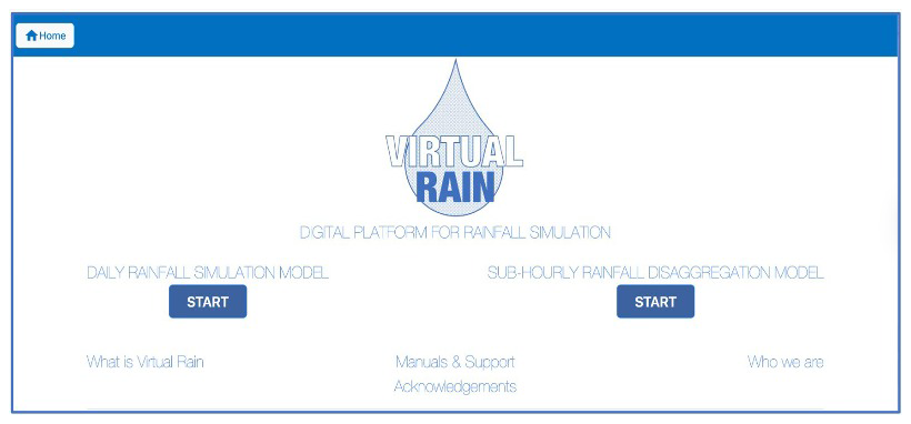
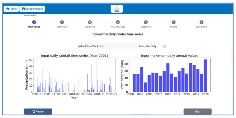
Figure A2 Input interface for uploading the observed daily rainfall time series, including visualization of the first year and annual daily maxima.

The Appendix is organized according to the two modules introduced in Sect. 3.1:

• Module 1: Daily rainfall stochastic simulation;

• Module 2: Sub-hourly rainfall disaggregation.

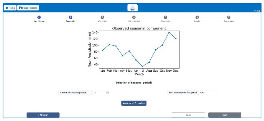
Figure A3 Seasonality interface supporting the user-defined selection of the number of seasonal periods and the starting month. The seasonal partition is specified by the user and is not automatically determined by the software.

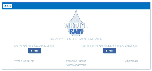
Figure A1 shows the initial access interface of the platform, from which the user can select one of the two rainfall models and start the modelling workflow.

A1 Module 1 – daily rainfall simulation

Figure A2 reports the upload interface for the observed rainfall data together with the first exploratory diagnostics, including daily rainfall variability and annual maxima. These preliminary outputs allow the user to visually inspect the rainfall series before starting the stochastic modelling workflow.

Figure A3 illustrates the interface used to define the seasonal partitioning of the rainfall series based on the monthly seasonal component plot automatically generated by the platform. This step represents a key modelling choice, since the selected seasonal aggregation directly affects both the fitting of marginal distributions and the calibration of the autocorrelation structures.

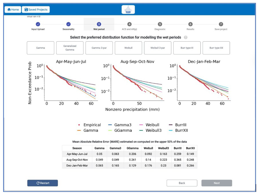
Figure A4 Wet period module: calibration results of marginal distributions for non-zero rainfall values.

Figure A4 shows the calibration results of the candidate marginal distributions fitted to wet-day rainfall values for each seasonal group. Both graphical and tabular outputs are provided to support the user in selecting the most appropriate marginal distribution according to the fitting performance and the reproduction of the upper-tail behavior.

Figure A5 ACS and AR(p) interface: calibration results of the autocorrelation structure.

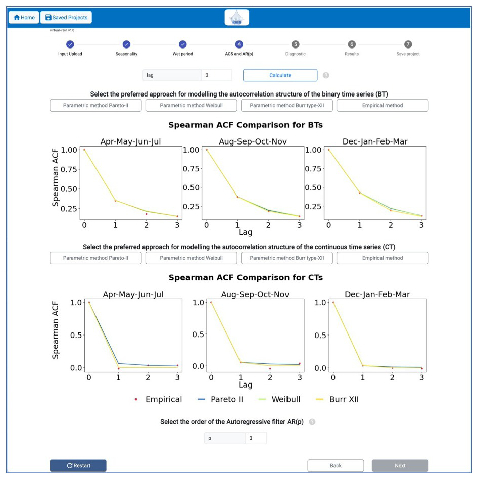
Figure A5 reports the ACS calibration for both the binary and continuous rainfall processes based on the number of lags specified by the user. The interface allows the comparison between empirical and fitted Spearman ACSs obtained after calibration. At this stage, the user can select either the empirical ACS or the preferred parametric representation. The interface also allows the specification of the autoregressive order (p). It is important to note that, when the empirical ACS is selected, the number of lags necessarily coincides with the order (p) of the AR model.

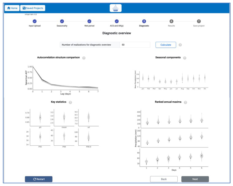
Figure A6 Diagnostic interface: comparison between observed and simulated statistical properties for model evaluation.

Figure A6 illustrates the diagnostic interface used to evaluate the consistency between observed and simulated rainfall statistics through ensemble-based comparisons. In this step, the user first specifies the number of synthetic daily time series to be generated. The quality of the simulations is then assessed by comparing observed and simulated properties, including: (i) autocorrelation structure, describing temporal dependence; (ii) seasonal cycle based on monthly mean rainfall; (iii) ranked annual maxima (highest, median and lowest); (iv) summary statistics, including dry-day probability (p0), mean wet-day rainfall, standard deviation, and extreme percentiles (P95, P99 and P99.9). These diagnostics support model diagnostic and help the user refine the modelling configuration when necessary.

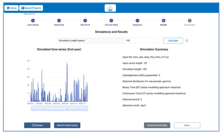
Figure A7 Results interface: visualization of the simulated series (first year) and summary of simulation settings.

Figure A7 presents the final output interface of Module 1, including the simulated rainfall series and a summary of the selected stochastic-model configuration. From this interface, the user can directly download the generated rainfall series or automatically transfer the simulated dataset to Module 2 for temporal disaggregation into sub-hourly resolutions.

A2 Module 2 – sub-hourly rainfall disaggregation

Figure A8 shows the input interface of the disaggregation module, where the user specifies the starting date of the uploaded rainfall time series together with the scaling exponent n, representing the slope of the IDF curves in logarithmic scale. This parameter is required for the calibration of the MRC model and controls the scaling relationship across temporal resolutions.

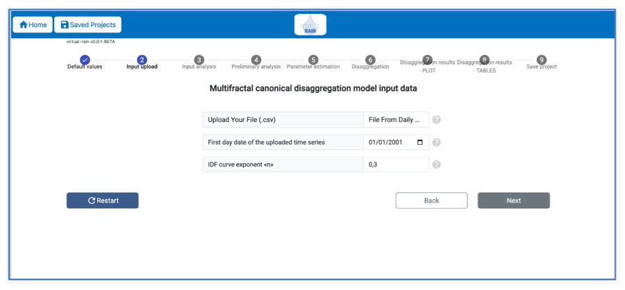
Figure A8 Input interface of the Sub-hourly Disaggregation Module showing the required inputs, including the starting date of the rainfall series and the IDF scaling exponent n.

Figure A9 reports the preliminary extreme-rainfall analysis, including the visualization of the first year of the rainfall series and the annual maximum daily rainfall values. The interface also provides the Gumbel plot comparing the empirical distribution of the a-coefficients with the fitted GEV distributions obtained using three estimation methods: Maximum Likelihood (MLE), Probability Weighted Moments (PWM), and L-moments (L-mom).

Figure A10 presents the estimated GEV parameters according to the method selected in the previous step, together with the mean annual rainfall intensity and the corresponding a-coefficients used as inputs for the MRC calibration procedure. The platform also allows the user to directly provide custom a-coefficients instead of estimating them from the observed rainfall series.

Figure A11 illustrates the calibration results of the MRC model, including the comparison between theoretical and empirical IDF curves for the selected return periods. The interface also reports the estimated MRC parameters resulting from the numerical optimization procedure and the corresponding objective-function value.

Figure A12 shows the interface used to configure the temporal disaggregation process, including the target temporal resolution (up to 1 min) and the number of stochastic realizations to be generated.

Figure A13 presents the graphical comparison between the observed daily rainfall series and the corresponding disaggregated sub-hourly realization generated by the MRC model.

Figure A14 reports a comprehensive summary of the statistical properties of the disaggregated rainfall series. The interface includes key indicators such as sample size, dry-period frequency, mean and standard deviation, extreme percentiles, maximum rainfall values at multiple aggregation scales, autocorrelation coefficients, and IDF-related parameters. These outputs provide a complete characterization of the generated time series and support the evaluation of its statistical consistency. This final step concludes Module 2 and allows the user to directly download the disaggregated rainfall series.

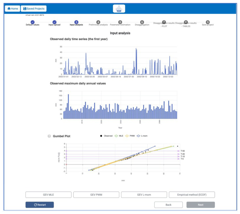
Figure A9 Preliminary analysis interface showing daily rainfall for the first year, annual maximum daily rainfall and the Gumbel plot comparing GEV fits obtained through MLE, PWM and L-mom methods.

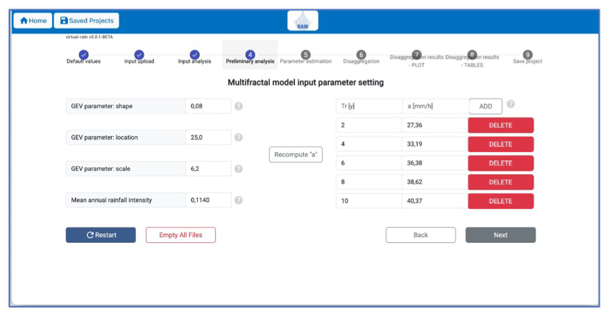
Figure A10 Interface reporting estimated GEV parameters, mean annual rainfall intensity and the a-coefficients associated with the selected return periods.

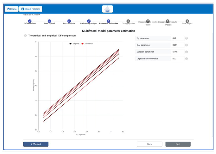
Figure A11 MRC calibration interface showing the comparison between imposed and calibrated IDF curves for the selected return periods, together with the estimated MRC parameters and objective-function value.

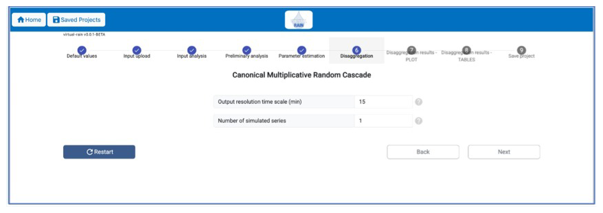
Figure A12 Disaggregation setup interface used to define the target temporal resolution and the number of stochastic simulations.

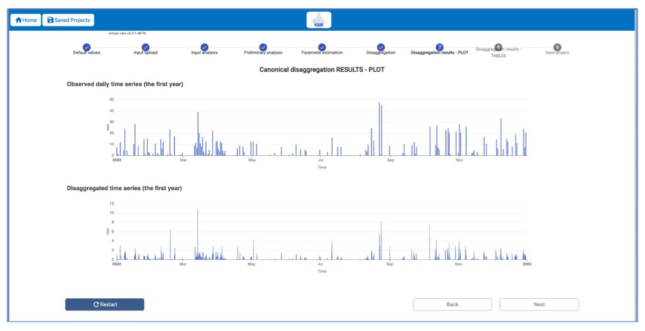
Figure A13 Disaggregation results interface showing the comparison between the observed daily rainfall series and the generated sub-hourly disaggregated series for the first simulation year.

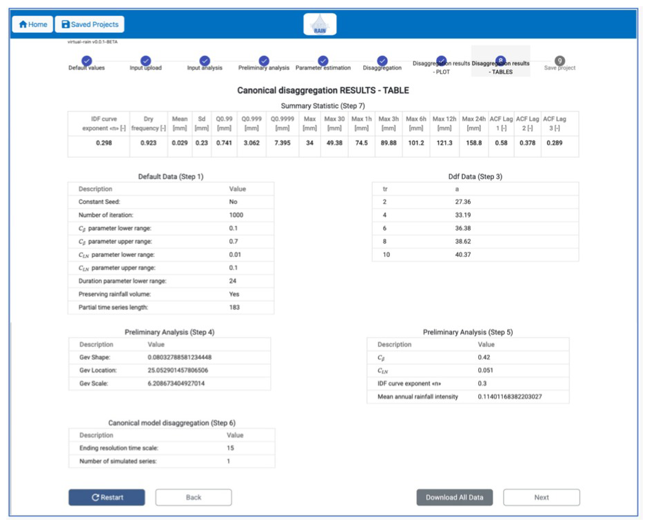
Figure A14 Summary table interface reporting the statistical properties of the disaggregated rainfall series together with the calibrated MRC parameters and IDF-related statistics.