Short-lived halogen sources and chemistry in the Community Earth System Model v2 (CESM2-SLH)

The implementation of short-lived halogen (SLH) sources and atmospheric chemistry in the Community Earth System Model v1 (CESM1) allowed to study the influence of SLH chemistry on the oxidative capacity of the atmosphere and, consequently, the Earth's climate. In this manuscript, we summarize 15 years of research on SLH chemistry and present a complete revision of the porting of the original developments into the latest version of CESM (v2), hereafter CESM2-SLH. This includes a detailed description of all offline and online sources of organic and inorganic SLH, as well as the gas-phase and heterogeneous recycling of chlorine, bromine and iodine in the troposphere and stratosphere, including their species-independent atmospheric sinks. In doing so, we provide a comprehensive evaluation of how changes in model parameters and coupled dynamics within the Community Atmosphere Model v6 (CAM6) affect SLH abundances and their implications. The new CESM2-SLH implementation offers various model configurations and resolutions, all of which result in equivalent global budgets and zonal distributions of organic and inorganic chlorine, bromine and iodine, which in turn, lead to SLH impacts on atmospheric composition that are consistent with previous CESM1 results. The released CESM2-SLH version includes specific namelist options, input files and technical notes detailing the most relevant SLH updates implemented in main CESM2/CAM6 routines. Our results show that the tropospheric halogen budget and tropical stratospheric injection of organic and inorganic chlorine, bromine and iodine species in CESM2-SLH are in agreement with observational assessments, resulting in significant global ozone reductions (−21 % to −28 % at the surface, −17 % to −22 % in the troposphere and up to −3 % in the stratosphere). Equivalent changes in OH and NO₂ abundance are also found, respectively ranging between −2 % to −9 % and −1 % to −10 %), depending on the specific model configuration and resolution. Based on this, we encourage the wider CESM community to consider the released CESM2-SLH scheme to obtain a more realistic representation of the background influence of natural and anthropogenic short-lived halogen sources and chemistry in air quality and Earth's climate studies.

1 Introduction

Over the past few decades, both observational and modelling studies have shown that Short-Lived Halogens (SLH) are widespread and ubiquitously distributed throughout the troposphere and stratosphere (Chance, 1998; Alicke et al., 1999; Saiz-Lopez et al., 2007; Read et al., 2008; Thornton et al., 2010; Prados-Roman et al., 2015a; Koenig et al., 2020). This SLH definition (Saiz-Lopez et al., 2023) includes the contribution from organic (i.e., carbon-bonded) very short-lived (VSL) halocarbons with a chemical lifetime smaller than 6 months plus the contribution of inorganic halogen species (collectively called Cl_y, Br_y and I_y for chlorine, bromine and iodine, respectively) that, through chemical cycling, partition between reactive and reservoir fractions within the gas-phase. Due to their short lifetime, reactive halogens affect atmospheric chemical composition including the depletion of tropospheric ozone (O₃), and consequently, the production of the hydroxyl radical (OH) and the partitioning between both hydrogen (HO₂/OH) and nitrogen (NO₂/NO) oxides (Saiz-Lopez and von Glasow, 2012). In addition, SLH compounds contribute to stratospheric ozone depletion (Salawitch et al., 2005; Sinnhuber et al., 2009), particularly over Antarctica where reactive bromine and iodine enhance the depth and size of the springtime ozone hole (Fernandez et al., 2017; Cuevas et al., 2022). Recently, SLH chemistry has been shown to influence the Earth radiative balance through direct and indirect chemical coupling with methane (CH₄) (Li et al., 2022), O₃ (Saiz-Lopez et al., 2023) and OH (Bossolasco et al., 2025), as well as the oxidation of dimethyl sulphide (DMS) and other sulphate sources which, in turn, can alter the formation of cloud condensation nuclei (Wohl et al., 2024).

VSL species are organic halogenated source gases (SGs) such as chloro-, bromo-, iodo-carbons which are present in the atmosphere in the form they were emitted. Bromine and iodine SGs are predominantly natural and emitted from the oceans (e.g., CHBr₃, CH₂Br₂ and CH₃I), whereas chlorine species such as CH₂Cl₂ and C₂Cl₄ have an important contribution from anthropogenic sources (WMO, 2022). The oceans are also the source of abiotic emission of hypoiodous acid (HOI) and molecular iodine (I₂) following the deposition of tropospheric ozone to the ocean surface and the reaction with iodide ions (Carpenter et al., 2013; MacDonald et al., 2014). This oceanic source of inorganic iodine is estimated to account for ∼75 % of the total source of atmospheric iodine, with the rest coming from VSL iodocarbons (Prados-Roman et al., 2015b). Similarly, very efficient heterogeneous reactions occurring at the surface of sea-salt aerosols (SSA) can result in the initial uptake and subsequent release of different halogen species within the Marine Boundary Layer (MBL), constituting a significant source of inorganic chlorine and bromine to the lower atmosphere, which is currently considered to be the dominant natural halogen source (WMO, 2018; Saiz-Lopez et al., 2023).

Once in the atmosphere, VSL SGs photo-decompose to release inorganic halogen product gases (PGs) that cycle back and forth between reactive (ClO_x, BrO_x and IO_x) and reservoir species, the whole group of which constitute SLH species. In contrast, long-lived Ozone Depleting Substances (ODSs), such as chloro-fluoro-carbons (CFCs) and brominated halons, remain unreactive throughout the troposphere until they are photodecomposed in the stratosphere (WMO, 2018, 2022). The photochemical cycling of SLH involves chemical reactions with other hydrogen, nitrogen, carbon and sulphur species, modifying the chemical composition of the atmosphere and therefore affecting its oxidative capacity and consequently, the Earth's climate (Li et al., 2022; Saiz-Lopez et al., 2023; Bossolasco et al., 2025). A detailed descriptions of the overall processes and reactions occurring in the atmosphere have been widely described in the literature (e.g., see the reviews of Saiz-Lopez and von Glasow, 2012; Simpson et al., 2015 and/or supplementary information of previous studies; Saiz-Lopez et al., 2014, 2023; Badia et al., 2021). Below we provide a brief description of the most relevant chemical cycles in which SLH participate.

The first step in the long reactive chain of SLH is the photochemical breakdown of either organic VSL halocarbons and/or photo-labile inorganic halogen species that results in the release of chlorine, bromine and iodine atoms, typically represented by X,Y = Cl, Br, I (Reactions R1a–R1c). Once in the atmosphere, these highly reactive halogen atoms (particularly I and Br) can catalytically destroy O₃, which in turn, controls the tropospheric formation of the OH radical through the reaction of O¹D with water vapour (Reactions R2–R4). Here, note that OH is typically referred to as the “atmospheric detergent” because it dominates the chemical decomposition of different volatile organic compounds (VOCs), and therefore controls the oxidative capacity of the troposphere (Reaction R5a). Similarly, direct reactions of halogen radicals (particularly Cl atoms) with several VOCs also contribute to the photochemical degradation of biogenic compounds and anthropogenic pollutants emitted to the atmosphere (Reactions R5b–R7), including CH₄. As a result, halogen chemistry alters the overall partitioning between nitrogen (NO_x = NO + NO₂) and hydrogen (HO_x = OH + HO₂) cycling (Reactions R8–R10), which has important implications for determining the chemical composition not only for halogens, but also for several reactive and reservoir species in the global atmosphere. Therefore, SLH chemistry can either increase the photochemical degradation rate of VOCs as well as the formation of aerosols (Saiz-Lopez and von Glasow, 2012; Simpson et al., 2015), while at the same time it can decrease the OH-driven chemical destruction and/or production rates due to their direct influence on O₃ abundance (Iglesias-Suarez et al., 2020; Badia et al., 2021; Saiz-Lopez et al., 2023), which in turn controls OH (Benavent et al., 2022; Bossolasco et al., 2025). Finally, it is worth noting that depending on the background environment, reactive halogen chemistry can also result in ozone production under polluted environments due to the formation of nitryl chloride (ClNO₂) that, through photolysis (Reaction R11), represents an additional source of NO_x (Reactions R12 and R13).

$$\begin{array}{}\text{(R1a)}& {\displaystyle }& {\displaystyle }\mathrm{CH}{X}_{\mathrm{3}}+h\mathit{\upsilon }\to \mathrm{3}X\text{(R1b)}& {\displaystyle }& {\displaystyle }{\mathrm{CH}}_{\mathrm{2}}XY+\mathrm{OH}\to X+Y\text{(R1c)}& {\displaystyle }& {\displaystyle }XY+h\mathit{\upsilon }/\mathrm{OH}\to X+Y\end{array}$$

$$\begin{array}{}\text{(R2)}& {\displaystyle }& {\displaystyle }X+{\mathrm{O}}_{\mathrm{3}}\to X\mathrm{O}+{\mathrm{O}}_{\mathrm{2}}\text{(R3)}& {\displaystyle }& {\displaystyle }{\mathrm{O}}_{\mathrm{3}}+h\mathit{\upsilon }\to {\mathrm{O}}^{\mathrm{1}}\mathrm{D}+{\mathrm{O}}_{\mathrm{2}}\text{(R4)}& {\displaystyle }& {\displaystyle }{\mathrm{O}}^{\mathrm{1}}\mathrm{D}+{\mathrm{H}}_{\mathrm{2}}\mathrm{O}\to \mathrm{2}\mathrm{OH}\end{array}$$

$$\begin{array}{}\text{(R5a)}& {\displaystyle }& {\displaystyle }\mathrm{OH}+\mathrm{VOCs}\to {\mathrm{RO}}_{\mathrm{2}}+{\mathrm{HO}}_{\mathrm{2}}\text{(R5b)}& {\displaystyle }& {\displaystyle }X/Y+\mathrm{VOCs}\to {\mathrm{RO}}_{\mathrm{2}}+\mathrm{H}X\end{array}$$

$$\begin{array}{}\text{(R6)}& {\displaystyle }& {\displaystyle }{\mathrm{RO}}_{\mathrm{2}}+\mathrm{NO}\to {\mathrm{NO}}_{\mathrm{2}}+\mathrm{RO}\text{(R7)}& {\displaystyle }& {\displaystyle }\mathrm{RO}+{\mathrm{O}}_{\mathrm{2}}\to {\mathrm{HO}}_{\mathrm{2}}+\mathrm{products}\text{(R8)}& {\displaystyle }& {\displaystyle }\mathrm{NO}+{\mathrm{HO}}_{\mathrm{2}}\to {\mathrm{NO}}_{\mathrm{2}}+\mathrm{OH}\text{(R9)}& {\displaystyle }& {\displaystyle }X\mathrm{O}+{\mathrm{HO}}_{\mathrm{2}}\to \mathrm{HO}X+{\mathrm{O}}_{\mathrm{2}}\text{(R10)}& {\displaystyle }& {\displaystyle }\mathrm{HO}X+h\mathit{\upsilon }\to X+\mathrm{OH}\text{(R11)}& {\displaystyle }& {\displaystyle }{\mathrm{ClNO}}_{\mathrm{2}}+h\mathit{\upsilon }\to \mathrm{Cl}+{\mathrm{NO}}_{\mathrm{2}}\text{(R12)}& {\displaystyle }& {\displaystyle }{\mathrm{NO}}_{\mathrm{2}}+h\mathit{\upsilon }\to \mathrm{NO}+{\mathrm{O}}^{\mathrm{3}}\mathrm{P}\text{(R13)}& {\displaystyle }& {\displaystyle }{\mathrm{O}}^{\mathrm{3}}\mathrm{P}+{\mathrm{O}}_{\mathrm{2}}+M\to {\mathrm{O}}_{\mathrm{3}}+M\end{array}$$

In this work, we describe the implementation of SLH chemistry into the Community Earth System Model, version 2 (CESM2) (Danabasoglu et al., 2020), which include version 6 of the Community Atmospheric Model (CAM6) physics (Gettelman et al., 2019a), as well as the tropospheric and stratospheric (TS1) chemistry scheme within CAM6-Chem (Emmons et al., 2020). The corresponding SLH implementation in the Whole Atmosphere Community Climate Model v6 (WACCM6) troposphere, stratosphere, mesosphere, and lower thermosphere (TSMLT1) chemical scheme (Gettelman et al., 2019b) has also been performed. The implementation is based on most of the previous SLH developments implemented in CESM1 from Saiz-Lopez et al. (2012) to Saiz-Lopez et al. (2023). Due to the changes in several atmospheric and oceanic fields between CESM1 and CESM2, such as sea surface temperature (SST), SSA and the corresponding aerosols surface area density (SAD) computation, as well as the different prescribed pollutant emissions, meteorological fields and/or atmospheric dynamics affecting SLH chemical cycling, transport and washout in the atmosphere (Gettelman et al., 2019a; Danabasoglu et al., 2020; Emmons et al., 2020; Simpson et al., 2023), we have included a new user-defined namelist section including a set of scaling-factors that allows CESM2-SLH performance to be consistent with the previous version of the model.

The paper is organized as follows: Sect. 2 describes the implementation of SLH chemistry in CESM, while Sect. 3 introduces the new CESM2-SLH configurations available and the complete set of experiments performed. Then, in Sect. 4 we present a comprehensive description of SLH global abundances and distributions obtained with the new CESM2-SLH model and how they compare with previous CESM1 results as well as with observations. Finally, Sects. 5 and 6 presents, respectively, a discussion of the results variability obtained with different model configurations and the importance of considering SLH chemistry in CESM as well as in other chemistry-climate models. We also provide a technical Appendix with several suggestions and notes of caution for new CESM2-SLH users, emphasising the need and types of model validation checks that must be performed in case other configurations beyond the ones described here are used.

2 Implementation of SLH chemistry in CESM

Although not strictly chronological, below we provide a brief description of the most important SLH developments originally implemented in CESM1 (CAM4-Chem). We begin with the initial descriptive papers that presented the main sources, reactions and halogen species, then continue with the subsequent updates and improvements, and finalize with the latest modelling studies that have demonstrated the importance of considering SLH chemistry to improve our understanding of atmospheric chemistry, air quality and climate evolution from past, to present and future. All these developments, have been led by the Atmospheric Chemistry and Climate group (AC2, IQF-CSIC, Madrid, Spain), in close cooperation with the Atmospheric Chemistry Observations & Modeling Department (ACOM-NCAR, Boulder, Colorado) and the Institute for Interdisciplinary Science (ICB-CONICET/UNCUYO, Mendoza, Argentina), as well as with fundamental contributions from other research groups around the world. Most of previous research used the term VSL or VSLS to refer to organic halogenated very short-lived substances. However, in this work we follow the most recent and complete representation of short-lived halogens in CESM (Saiz-Lopez et al., 2023), and therefore expanded the terminology to SLH, which includes in addition to VSLS, those inorganic halogen species (Cl_y, Br_y and I_y) that rapidly interconvert between each other and are responsible for the halogen impacts in the atmosphere. A comprehensive review of the SLH influence on atmospheric chemistry and climate is provided in Saiz-Lopez et al. (2025b).

The initial description of SLH halogen chemistry in CAM-Chem was published in Ordóñez et al. (2012), who presented a complete set of tables with all photochemical processes considered and also developed the VSL halocarbon emission inventory that was used in all subsequent studies. The companion work of Saiz-Lopez et al. (2012) performed the first estimation of the impacts of combined SLH (chlorine, bromine and iodine) on tropospheric ozone and radiative balance. Here, we acknowledge that these initial works considered offline inorganic iodine emissions. Afterwards, Prados-Roman et al. (2015a, b) implemented the online computation of oceanic iodine emissions and determined the negative geophysical feedback with tropospheric ozone that led to the hypothesis that atmospheric iodine levels would have tripled since the onset of the Industrial Era, later confirmed by ice-core observations (Cuevas et al., 2018). Further updates related mostly to heterogeneous recycling processes occurring in the MBL, Free Troposphere (FT) and Upper Troposphere (UT), relevant for properly quantifying the contribution of SLH to the stratospheric halogen loading of bromine (Fernandez et al., 2014) and iodine (Saiz-Lopez et al., 2014, 2015), led to quantification of the overall impact of natural bromine and iodine over the Antarctic ozone hole (Fernandez et al., 2017; Cuevas et al., 2022), as well as the seasonal variability within the mid-latitudes (Barrera et al., 2020). These updates included the online implementation of SSA-dehalogenation sources which are of particular importance for improving BrO observations in the MBL (Koenig et al., 2017), as well as the inclusion of higher order iodine oxides (I_xO_y), whose effective photolysis was found to be necessary to reproduce iodine observations in the upper troposphere and lower stratosphere (Saiz-Lopez et al., 2014, 2015; Koenig et al., 2020). For the particular case of chlorine, the contribution of anthropogenic VSLS was implemented based on the emissions inventories from Hossaini et al. (2019) and Claxton et al. (2020), with further updates related to the inorganic chlorine emissions resulting from the heterogeneous recycling of nitrogen oxides and nitric acid on chloride-rich aerosols, the so called acid-displacement reactions (Li et al., 2022). These allowed to evaluate for the first time the combined impact of halogens (chlorine, bromine and iodine) over tropospheric ozone during the 21st century (Iglesias-Suarez et al., 2020; Badia et al., 2021) in comparison with pristine pre-industrial conditions (Barrera et al., 2023); as well as the enhanced chemical coupling of natural and anthropogenic SLH on the lowermost tropical stratosphere ozone trends (Villamayor et al., 2023). Based on these works, and thanks to the implementation of CH₄ emission-driven simulations (Li et al., 2022) and polar halogen emissions from the sea-ice (Fernandez et al., 2019, 2024), SLH were demonstrated to induce an overall cooling effect on the climate system arising from the direct and indirect (and sometimes opposite) influence of reactive halogens on ozone, methane, aerosols and stratospheric water vapour (Saiz-Lopez et al., 2023). CESM1 simulations including SLH also enabled quantification of the radiative influence of DMS and methanethiol (MeSH) oceanic emissions on the direct sulphate aerosol radiative effect over the Southern Ocean (Veres et al., 2020; Wohl et al., 2024), while the overall influence of SLH on all tropospheric oxidants has recently been described in Bossolasco et al. (2025). The role of anthropogenic SLH emissions from biomass burning and other sources on long-term atmospheric chemistry and mercury contamination over continental Asia has also been evaluated using CESM1 (Chang et al., 2024; Fu et al., 2024). The model has been also employed to evaluate the potential of chlorine based interventions in climate mitigation through methane reduction (Li et al., 2023; Meidan et al., 2024), as well as to quantify for the first time the role of the stratosphere on the global mercury cycle and surface deposition (Saiz-Lopez et al., 2025a).

It is important to note that not all processes, reactions and implications summarized in previous studies have been implemented in the current release of CESM2-SLH described in this work. Please refer to Sect. 3.3 below for further details. It is worth noting that following the pioneering implementation of combined SLH emissions and chemistry into CAM4-Chem, other research groups implemented SLH schemes in different models, which in many cases followed the original implementation of SLH in CESM, particularly for iodine. These include global and regional models such as EMAC (Sinnhuber and Meul, 2015), TOMCAT (Hossaini et al., 2016), GEOS-Chem (Sherwen et al., 2016a, b), CMAQ (Sarwar et al., 2015), WRF-Chem (Badia et al., 2019), SOCOL (Karagodin-Doyennel et al., 2021) and LMDZ-INCA (Caram et al., 2023).

2.1 Short-lived halogen emissions

The starting point of SLH implementation in CESM was the development of an oceanic emission inventory of VSL halocarbons (Ordóñez et al., 2012), which not only represents an important tropospheric halogen source, but was also needed to reproduce total stratospheric bromine loading observations (WMO, 2018, 2022). To achieve this goal, many global models – including CESM1 and CESM2 – initially assumed a constant surface abundance of the two main bromocarbons – i.e., bromoform (CHBr₃) and dibromomethane (CH₂Br₂) – and imposed a Lower Boundary Condition (LBC) of 1.2 pptv each (adding up to 6 pptv of total bromine at the model surface), which resulted in an additional bromine stratospheric injection of approximately 5 pptv (Eyring et al., 2013; Hegglin et al., 2014). However, motivated by the rapid photochemical-degradation of VSLS in the troposphere, spatially- and temporally-resolved emission inventories were implemented to account for oceanic halocarbon emissions of bromine and iodine (which include mostly natural sources), and was later extended to chlorocarbons, for which the anthropogenic emissions dominate. These original VSLS oceanic sources, which represent the initial step releasing highly reactive Cl, Br and I atoms in the lower troposphere, were further extended by computing the online recycling of inorganic halogen sources occurring at the ocean surface as well as on sea-salt aerosols. Section 2.1.1 and 2.1.2 describe, respectively, the natural and anthropogenic sources of VSL halocarbons implemented in CESM2-SLH, while Sect. 2.1.3 describes the online recycling of halogen reservoirs that represent a net source of SLH to the atmosphere.

2.1.1 Natural offline halocarbon emissions

The implementation of VSL halocarbons emitted from the ocean in CESM has been described in Ordóñez et al. (2012). The methodology follows a top-down approach based on chlorophyll-a monthly climatology from the SeaWIFS project for the 1998–2003 period (Melin, 2013), and the iterative adjustment of emission flux strength by comparing modelled distributions and vertical profiles of VSL halocarbons with a compilation of aircraft campaigns and surface observations (see Tables 1 and 2 in Ordóñez et al., 2012). Nine halogenated VSL species are included in the Ordóñez et al. (2012) emission inventory, including individual emissions of two bromocarbons (CHBr₃ and CH₂Br₂), three bromo-chlorocarbons (CH₂BrCl, CHBrCl₂ and CHBr₂Cl), two iodocarbons (CH₃I and CH₂I₂), one iodo-chloro (CH₂ICl) and another iodo-bromo (CH₂IBr) carbon, respectively. All of these species are well known to be emitted from biologically active oceans as side products of the metabolite of different micro- and macro-algae and phytoplankton colonies (Carpenter and Liss, 2000; Carpenter et al., 2003). In the Ordóñez et al. (2012) inventory, the oceanic emission shows a seasonal and latitudinal distribution, with most of the emission (∼70 %) occurring in the tropics (20° N–20° S), approximately 25 % arising from the north and south mid-latitudes (20–50° on both hemispheres) and the remaining 5 % released from ice-free oceanic regions from the high-latitudes and polar regions. The net oceanic emission flux of each halocarbon species (E_spec) is given by Eq. (1);

$$\begin{array}{}\text{(1)}& E_{\mathrm{spec}}=\mathrm{1.127}\times {\mathrm{10}}^{\mathrm{5}}\times f_{\mathrm{spec}}\times r_{\mathrm{coast}}\times {\mathrm{chl}}_a,\end{array}$$

where f_spec is a species-dependent scaling factor iteratively adjusted to improve model-observation agreement, r_coast is a constant enhancement factor applied only to coastal areas outside the tropics, and chl_a is the SeaWIFS monthly climatology chlorophyll-a distribution (Ordóñez et al., 2012). In comparison to other VSLS approaches considering only latitudinal bands (Warwick et al., 2006a, b; Butler et al., 2007; Jones et al., 2010), the Ordóñez et al. (2012) inventory introduces a tropical geographically-heterogeneous and seasonally dependent variability, which allows for an improved spatio-temporal representation of VSLS distribution in the global troposphere. Once the monthly-mean prescribed fields are read, hourly dependent profiles are applied to the flux strength of all halocarbons to represent the photosynthetic dependence on radiation intensity. Therefore, VSLS emissions follow a Gaussian diurnal profile with peak emissions at local solar noon (Ordóñez et al., 2012), with exception of CH₂I₂ that follows a top-hat shape with a uniform distribution during the day and no-null emissions at night (see Fig. S1 in the Supplement). Given that no global long-term trend has been observed or established (WMO, 2022; Tinel et al., 2023), the emission strength of oceanic halocarbons is assumed to follow a constant climatology.

Due to improvements in the representation of large-scale ascent and transport across the boundary layer in CESM2 (Simpson et al., 2020) as well as in the emission strength and speciation of air pollutants altering the oxidative capacity of the troposphere (Emmons et al., 2020) the original Ordóñez et al. (2012) inventory for chlorinated and brominates species was increased by a constant factor of 1.15 (i.e., 15 %) to reproduce the stratospheric halogen loading obtained in previous CESM1 studies (Fernandez et al., 2014, 2021). The rationale for increasing the offline emission fluxes is that the reduction of transport across the boundary layer and the increase near-surface OH abundance in CESM2-SLH results in more efficient conversion from SGs to PGs at lower model levels. Given the much shorter photochemical lifetime of iodine species, no scaling was applied to VSL iodocarbons.

2.1.2 Anthropogenic offline halocarbon emissions

For anthropogenic VSL sources of chlorocarbons, we used the Hossaini et al. (2019) and Claxton et al. (2020) emission inventories, which include time-dependent emission of two major contributors to the organic chlorine load (CH₂Cl₂ and C₂Cl₄.) as well as surface LBCs for two other compounds (CHCl₃ and C₂H₄Cl₂) during the recent past. Beside a fraction of CHCl₃ emissions arise from natural sources (with minor contributions from the other compounds), chlorinated VSLS are dominated by anthropogenic emissions that display a pronounced hemispheric asymmetry (WMO, 2022). Therefore, hereafter we assume all of these offline emissions to have only an anthropogenic origin. Consistent with the scaling factor applied to the Ordóñez et al. (2012) inventory, both VSL chlorocarbon surface emissions and LBCs were globally scaled by the same constant factor (1.15 or 15 % enhancement). It should be noted that additional anthropogenic halocarbon sources, as those arising from the waste treatment of power-plants as well as seaweed aquaculture are not considered (Carpenter et al., 2000; Leedham et al., 2013; Jia et al., 2023).

2.1.3 Online emissions of inorganic halogens

In addition to the VSL halocarbon emissions, abiotic sources of inorganic halogens are implemented in the model. Here it is worth noting that these ocean-related sources have different routes for iodine compared to bromine and chlorine, and therefore are described separately. Inorganic iodine (HOI and I₂) emissions from the ocean surface are computed online following the ozone-driven oxidation of aqueous iodide occurring at the seawater surface (Carpenter et al., 2013). Following Prados-Roman et al. (2015b), the parameterized expressions for HOI and I₂ fluxes from MacDonald et al. (2014) are computed online by Eqs. (2a) and (b), respectively,

$$\begin{array}{}\text{(2a)}& {\displaystyle }\begin{array}{rl}{F}_{\mathrm{HOI}}& =\left[{\mathrm{O}}_{\mathrm{3}}\right]\times (\mathrm{4.15}\times {\mathrm{10}}^{\mathrm{5}}\times \sqrt{{\displaystyle \frac{\left[{\mathrm{I}}_{\mathrm{aq}}^{-}\right]}{w}}}-\left({\displaystyle \frac{\mathrm{20.6}}{w}}\right)\\ & -\mathrm{23}\mathrm{600}\times \sqrt{\left[{\mathrm{I}}_{\mathrm{aq}}^{-}\right]}),\end{array}\text{(2b)}& {\displaystyle }\begin{array}{rl}{F}_{{\mathrm{I}}_{\mathrm{2}}}& =\left[{\mathrm{O}}_{\mathrm{3}}\right]\times {\left[{\mathrm{I}}_{\mathrm{aq}}^{-}\right]}^{\mathrm{1.3}}\times (\mathrm{1.74}\times {\mathrm{10}}^{\mathrm{9}}-(\mathrm{6.54}\times {\mathrm{10}}^{\mathrm{8}}\\ & \times \ln \left(w\right)\left)\right),\end{array}\end{array}$$

where [O₃] and w are the surface ozone abundance (ppbv) and wind speed (m s⁻¹), respectively, computed over the ocean at the lowest model level. [I${}_{\mathrm{aq}}^{-}$] is the aqueous iodide seawater concentration computed by Eq. (2c), which in turn depends on the model SST,

$$\begin{array}{}\text{(2c)}& \left[{\mathrm{I}}_{\mathrm{aq}}^{-}\right]=\mathrm{1.46}\times {\mathrm{10}}^{\mathrm{6}}\times \exp \left({\displaystyle \frac{-\mathrm{9134}}{\mathrm{SST}}}\right).\end{array}$$

Equations (2a, b) are only valid for w≥3 m s⁻¹. Below this threshold, anomalously high iodine fluxes are obtained. To avoid this overprediction, w=3 m s⁻¹ is assumed for all grid cells where w<3 m s⁻¹. Not imposing this wind speed mask result in an overestimation of iodine fluxes from the ocean during calm periods (Inamdar et al., 2020). The first order dependence on ozone abundance of F_HOI and $F_{{\mathrm{I}}_{\mathrm{2}}}$ (Eqs. 2a and b) has important consequences for the long-term trend of inorganic iodine emissions during the historical period (see Sect. 4).

For bromine and chlorine, additional abiotic inorganic sources arise from the so-called SSA-dehalogenation reactions. In this case, the online computation of inorganic halogen emissions assumes an oxidized gas-phase species to be deposited on the sea-salt aerosol surface, followed by an heterogeneous reaction that captures a reduced halide reservoir within the substrate that is oxidized before being released to the gas-phase (Fernandez et al., 2014). This complex redox process is parameterized to proceed in a single-step heterogeneous reaction dependent on the collisional frequency of the gas-phase species and the substrate, as well as on the degassing efficiency of the halogenated product released to the atmosphere (Ordóñez et al., 2012). Given that CESM2 does not include an explicit treatment of aqueous phase chemistry and diffusion, we assume the rate-limiting step is the uptake of inorganic halogen species onto SSA and computes the first-order reaction rate based on the Free-Regime Approximation (FRA) approach (McFiggans et al., 2000) following

$$\begin{array}{}\text{(3)}& \begin{array}{rl}{F}_{\mathrm{SSA}}^{XY}& ={\displaystyle \frac{\mathrm{1}}{\mathrm{4}}}\times {\mathit{\gamma }}_{\mathrm{ox}}\times \left(\mathrm{100}\times \sqrt{{\displaystyle \frac{\mathrm{8}\times R\times T}{\mathit{\pi }\times {\mathrm{MW}}_{\mathrm{ox}}}}}\right)\times {\mathrm{SAD}}_{\mathrm{SSA}}\\ & \times \left[{\mathrm{Spec}}_{\mathrm{ox}}\right]\times \mathrm{DF}\times {\mathrm{mask}}_{\mathrm{SSA}}.\end{array}\end{array}$$

Here, $F_{\mathrm{SSA}}^{XY}$ is the flux of inorganic halogens (in the form of X₂ or XY, with X,Y = Cl, Br or I) in molec. cm⁻³ s⁻¹, γ_ox represents the accommodation coefficient of the gas-phase halogenated oxidized reservoir colliding with the SSA, MW_ox is the molecular weight (g mol⁻¹) of the oxidized species used to compute the mean-root square molecular speed, which in turn depends on the modelled temperature at each gridpoint (T in K) and the universal gas constant (R). Furthermore, the surface area density of SSA (SAD_SSA in cm⁻² cm⁻³) is computed considering the three SSA bins represented in the model, while [Spec_ox] is the atmospheric molecular concentration (molec. cm⁻³) of the gas-phase oxidized halogen species (XONO₂, XNO₂ and/or HOX, with X = Cl, Br and I) colliding with SSA. Finally, DF is a seasonal-dependent normalized depletion factor that represents the efficiency of the recycling reaction for any given atmospheric condition (Yang et al., 2005), while mask_SSA is a logical mask that limits the occurrence of the SSA-dehalogenation processes below a pressure threshold (P<300 hPa). Further details on the SSA-dehalogenation implementation in CESM can be found elsewhere (Ordóñez et al., 2012; Fernandez et al., 2014, 2021).

The FRA implementation in CESM2-SLH assumes that the bromide and chloride content of SSA is sufficiently large to act as an effectively infinite halide reservoir capable of sustaining the surface heterogeneous-redox reaction. This implies that the bromide and/or chloride content in the SSA bulk is always in excess compared to the abundance of the gas-phase halogen reservoir that deposits on the aerosol surface, which is valid for fresh SSA typically found close to the ocean surface. Therefore, the implementation of SSA-dehalogenation does not account for the slowing down of the halogen recycling when aged sea-salt aerosols become depleted in bromide and chloride (von Glasow et al., 2002). Table 1 summarizes all 9 independent reactions releasing either gas phase X₂ or XY, where the non-stoichiometric coefficients between reactants and products for each gas-phase halogen species determines the net inorganic halogen flux. Given the large increase in SSA abundance and vertical distribution between CESM1 and CESM2 (see Fig. S2), particularly over the boundary layer where the latter show up to 10 times larger values than the former, the accommodation coefficients (γ_ox) for halogenated reservoirs compiled in Table 4 of the Supplement of Ordóñez et al. (2012) was reduced by a factor of 3 for chlorine and iodine and by a factor of 8 for bromine (see Table 1). This scaling factors are within the reported uncertainty and variability of γ_ox for the different halogen families and aerosol compositions (Burkholder et al., 2020) and allowed to reproduce previously estimated SSA-dehalogenation fluxes and burdens (see Sect. 4.2).

Table 1 Heterogeneous recycling processes representing a net source of inorganic halogens in CESM2-SLH.

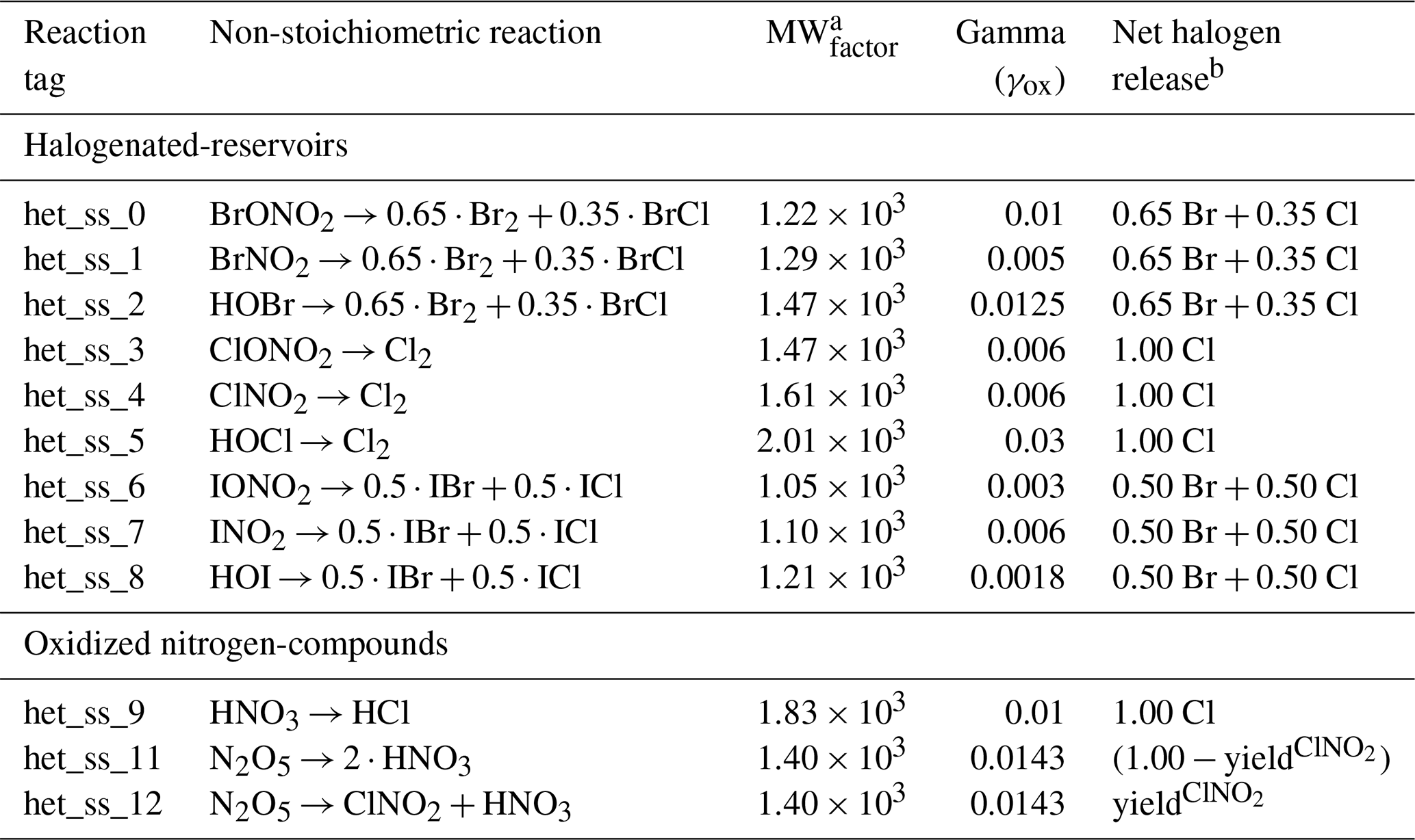
^a Values for the molecular weight factor (MW_factor) correspond to the following term from Eq. (3), $\left(\sqrt{\frac{\mathrm{8}\times R}{\mathit{\pi }\times {\mathrm{MW}}_{\mathrm{ox}}}}\right)$, where temperature has been excluded from the square-root and is later multiplied by an independent ($\sqrt{T}$) term. ^b The ClNO₂ yield is computed as yield${}^{{\mathrm{ClNO}}_{\mathrm{2}}}={\left(\frac{{\mathrm{SSA}}_{\mathrm{mass}}-{\mathrm{SSA}}_{\min }}{{\mathrm{SSA}}_{\max }-{\mathrm{SSA}}_{\min }}\right)}^{\mathrm{3}}$, where SSA_mass is the total sea-salt aerosol mass mixing ratio (kg kg⁻¹) of all aerosol bins in each model gridbox, while SSA${}_{\min }=\mathrm{5.0}\times {\mathrm{10}}^{-\mathrm{10}}$ and SSA${}_{\max }=\mathrm{1.0}\times {\mathrm{10}}^{-\mathrm{9}}$ are the minimum and maximum SSA_mass adjusted thresholds for N₂O₅ → 2 ⋅ HNO₃ implemented in Lamarque et al. (2012).

For chlorine, additional inorganic halogen sources arise from the heterogeneous recycling of nitrogen species (N₂O₅ and HNO₃) on halide-rich SSA (see Eq. 3 and Table 1). In the first case, the SSA uptake and recycling of N₂O₅ drives two key processes: (i) the well-documented hydrolysis to produce HNO₃ (het_ss_11, Lamarque et al., 2012); and (ii) the production of nitryl chloride (ClNO₂), which constitutes a net chlorine source (het_ss_12). The latter is of importance as ClNO₂ photolysis in polluted environments lead to ozone production (Knipping and Dabdub, 2003; Thornton et al., 2010). Within CESM2-SLH, the ClNO₂ yield is computed online based on a cubic expression dependent on the total sea-salt aerosol mass within each of the sea-salt aerosol bins (Li et al., 2022). In the second case (het_ss_9), the acid-displacement reaction results in the oxidation of the available chloride in the sea-salt bulk and depends on a fixed HNO₃ accommodation coefficient (Sander, 2015), following other models including chlorine chemistry (Hossaini et al., 2016). The implementation of both chlorine sources follows the FRA-approach described above for oxidized halogen reservoirs (Eq. 3), although in this case the uptake of oxidized nitrogen species drives the SSA-dehalogenation. We note that stoichiometric N₂O₅ recycling on halide-poor tropospheric aerosols is also considered in the model, although for these reactions the halogen uptake and recycling only constitute a partitioning shift between different halogen and nitrogen species (see Table 2).

Table 2 Heterogeneous recycling processes representing a change in partitioning of inorganic halogens in CESM2-SLH.

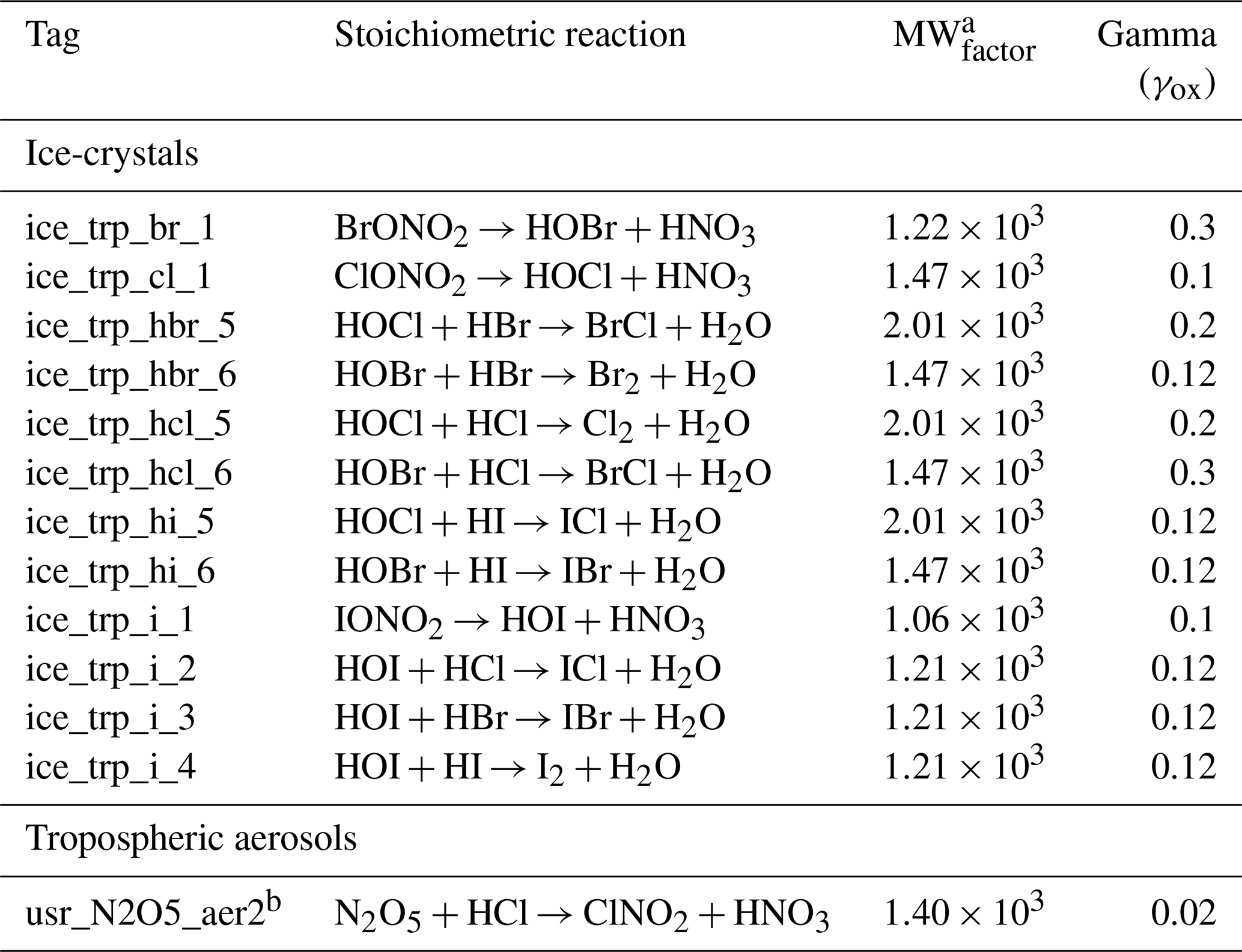
^a Values for the molecular weight factor (MW_factor) correspond to the following term from Eq. (3), $\left(\sqrt{\frac{\mathrm{8}\times R}{\mathit{\pi }\times {\mathrm{MW}}_{\mathrm{ox}}}}\right)$, where temperature has been excluded from the square-root and is later multiplied by an independent ($\sqrt{T}$) term. ^b A reaction yield of 0.138 is considered for ClNO₂ production (Li et al., 2022).

Finally, we highlight the importance of adjusting the strong model dependence of online SLH sources and burdens depending on the sea-salt abundances and distributions represented in different model configurations (see Fig. S2). Note that the accommodation coefficients (γ) and depletion factors (DF) altering the reactive efficiency for the different species reported in the literature (Sander, 2015; Burkholder et al., 2020) possess a wide range of values and large uncertainties that depend on variables that are unconstrained in the simplified parameterization implemented in CESM2-SLH (e.g., pH dependence, halide content, etc.). Consequently, variations in SSA fields, pollutant emissions, and atmospheric composition (e.g., HO_x/NO_x partitioning), combined with non-linear heterogeneous recycling (Table 1), may cause regional over-/under-estimations of halogen content in localized regions in comparison with previous CESM1 studies (see Sect. 5).

2.2 Short-lived halogen chemistry

In the following subsections, we provide a self-contained description of the main photochemical (Sect. 2.2.1), gas-phase (Sect. 2.2.2) and heterogeneous-phase (Sect. 2.2.3) reactions implemented in the default CESM2-SLH chemical scheme. This scheme builds upon the TS1.2 benchmark chemical mechanism used in CESM2 (Emmons et al., 2020), which explicitly includes the volatility basis set (VBS) parameterization for secondary organic aerosol formation (Tilmes et al., 2019, 2023). The complete set of SLH reactions added to the TS1-simpleVBS branch within the precompiled trop_strat_mam4_slh chemical pre-processor (chem_mech.in) is included in the Supplement (Tables S1–S3). An equivalent SLH chemical scheme has also been merged into the TSMLT1 mechanism for WACCM (waccm_tsmlt_mam4_slh).

2.2.1 Photochemical reactions

A comprehensive list of all photochemical halogen reactions included in the SLH scheme is shown in Table S1, based on the original publication compiled in Ordóñez et al. (2012) and Saiz-Lopez et al. (2014), with further updates from Badia et al. (2021) and Saiz-Lopez et al. (2023). This includes 11, 10 and 17 new photolysis reactions for chlorine, bromine and iodine, respectively, which adds up to previously defined photolysis reactions of long-lived halocarbons as well as odd-chlorine and odd-bromine reactions that are required for properly representing stratospheric ozone depletion in CESM2 (Gettelman et al., 2019b). The absorption cross sections and quantum yields are taken from the latest JPL 19-5 (Jet Propulsion Laboratory; Burkholder et al., 2020) and IUPAC (International Union of Pure and Applied Chemistry; Atkinson et al., 2007, 2008) handbooks, and are included within the xs_long and xs_short file typically used in CAM-Chem and WACCM. Wavelength integrated J-values are computed as a function of temperature and height considering the model actinic flux and a Look-Up-Table (LUT) approach (Kinnison et al., 2007; Lamarque et al., 2012; Emmons et al., 2020).

Note that the photodegradation of anthropogenic VSLS (CHCl₃, CH₂Cl₂ and C₂Cl₄) results in the formation of phosgene (COCl₂), which constitutes a halogen intermediate that accumulates in the upper troposphere until it photo-decomposes in the lower stratosphere (see Fig. S3) (Hossaini et al., 2016). Therefore, phosgene does not participate in direct ozone destruction in the lower-stratosphere until it releases the Cl atoms through photolysis. However, and given that the only source of phosgene in the model is the degradation of chlorinated VSLS, we consider the contribution of COCl₂ within the PGs chlorine fraction, in line with the latest WMO (2022) report. In addition, we follow the JPL 19-5 recommendation (Burkholder et al., 2020) of neglecting the C₂Cl₄ absorption cross-section beyond λ>270 nm (Keller-Rudek et al., 2013), as not doing so resulted in a complete photodecomposition in the lower troposphere which is not in line with observations (Roozitalab et al., 2024). For iodine, Table S1 considers the photodissociation of higher order oxides (I_xO_y, with x=2 and $y=\mathrm{2},\mathrm{3},\mathrm{4}$). The absorption cross sections of these species were derived from solution spectrum measured at the University of Leeds (Lewis et al., 2020), which were subsequently scaled to estimate absolute absorption cross-sections (Gómez Martín et al., 2005). Therefore, and supported by observationally-constrained modelling studies demonstrating that considering I_xO_y photolysis was required to reproduce gas-phase (Saiz-Lopez et al., 2014, 2015) and particulate iodine (Koenig et al., 2020) vertical profiles, the released CESM2-SLH chemical mechanism is based on the $J_{{\mathrm{I}}_x{\mathrm{O}}_y}$ scheme for iodine proposed in Saiz-Lopez et al. (2014).

2.2.2 Gas-phase reactions

A complete description of all bimolecular Arrhenius type reactions of halogen species are shown in Table S2, where for the sake of simplicity we have ordered reactions in the following groups: Odd-Oxygen, Odd-Chlorine, Odd-Bromine, Odd-Iodine, VSLS degradation and reactions with sulphur and carbon compounds. All these developments have been initially described in Ordóñez et al. (2012), with additional updates for iodine described in Saiz-Lopez et al. (2014). In addition, all termolecular reactions considered in the default SLH chemical mechanism are shown in Table S3. Note that for the final implementation of SLH chemistry in CESM2, all expressions, reaction-rate coefficients and temperature dependence factors have been updated to the reported values in the last JPL 19-5 handbook (Burkholder et al., 2020).

Oxidation of DMS to produce sulphur dioxide (SO₂) by BrO, Cl and IO are also included in the updated SLH chemical scheme. These improvements in sulphur chemistry representation in CESM2 with respect to CESM1, including tropospheric sulphate formation and washout, are a major source of uncertainty for radiative forcing estimations (Ge et al., 2022) and are currently under development. Therefore, the current CESM2-SLH mechanism has been developed starting from the benchmark sulphur scheme implemented in TS1.2 (Emmons et al., 2020). Similarly, the Modal Aerosol Model with 4 modes (MAM4) scheme is the default aerosol option in CESM2, which includes updates in the formation and growth of sulphate, black carbon and organic matter, secondary organic aerosols, sea salt, and dust (Liu et al., 2016). Although no direct SLH changes to the MAM4 scheme were implemented, we note that indirect perturbations of reactive halogens on OH abundance can influence the global aerosol burden (Saiz-Lopez et al., 2023). In the following section, we describe the stoichiometric heterogeneous processes involving inorganic halogens species.

2.2.3 Heterogeneous reactions

Heterogeneous SLH reactions occurring on different types of atmospheric substrates have also been implemented (see Table 2). It is worth noting that unlike the SSA-dehalogenation source described in Sect. 2.1.3, all of these reactions are stoichiometric and therefore do not represent a net halogen source from the aerosol to the gas-phase, but instead, result in a change in individual species partitioning between gaseous reactants and products. Indeed, in all cases, the substrate surface (e.g., ice-crystals, cloud droplets and/or other anthropogenic aerosols typically considered in CAM6 like black-carbon, organic carbon, sulphate, nitrate, etc.) acts like a catalyst and does not contribute with any halogen content. For heterogeneous reactions occurring over ice-crystals, we use the FRA approach to compute the reaction rate constant (rate_ice) considering the total number of gas-phase species that suffer uptake on the aerosol surface, resulting in the following expressions for uni-molecular

$$\begin{array}{}\text{(4a)}& \begin{array}{rl}{\mathrm{rate}}_{\mathrm{ice}}^{\mathrm{uni}}& ={\displaystyle \frac{\mathrm{1}}{\mathrm{4}}}\times {\mathit{\gamma }}^X\times \left(\mathrm{100}\times \sqrt{{\displaystyle \frac{\mathrm{8}\times R\times T}{\mathit{\pi }\times {\mathrm{MW}}_X}}}\right)\times {\mathrm{SAD}}_{\mathrm{ice}}\\ & \times {\mathrm{mask}}_{\mathrm{ice}}^{\mathrm{strat}},\end{array}\end{array}$$

and bimolecular

$$\begin{array}{}\text{(4b)}& \begin{array}{rl}{\mathrm{rate}}_{\mathrm{ice}}^{\mathrm{bi}}& ={\displaystyle \frac{\mathrm{1}}{\mathrm{4}}}\times {\mathit{\gamma }}^X\times \left(\mathrm{100}\times \sqrt{{\displaystyle \frac{\mathrm{8}\times R\times T}{\mathit{\pi }\times {\mathrm{MW}}_X}}}\right)\times {\mathrm{SAD}}_{\mathrm{ice}}\\ & \times {\mathrm{mask}}_{\mathrm{ice}}^{\mathrm{strat}}\times {\displaystyle \frac{\mathrm{1}}{\left[Y\right]}},\end{array}\end{array}$$

reactions (see Table 2). Here, γ^x and MW_X are, respectively, the accommodation coefficient and the molecular weight of the gas-phase halogenated reservoir species (X) that is initially taken up by the ice-crystal, SAD_ice represents the surface area density of ice crystals and is computed online based on the ice-water content in clouds (CLDICE) from the CAM6 model, and mask${}_{\mathrm{ice}}^{\mathrm{strat}}$ is a logical mask imposed to limit the computation below the model tropopause and avoid double-counting recycling reactions historically implemented to occur in the stratosphere (Kinnison et al., 2007; Fernandez et al., 2014). For bimolecular reactions, note that the reaction rate is normalized by the atmospheric concentration of the most abundant halogenated species (either X or Y) involved in the reaction. The original implementation of these reactions has been described in detail in Fernandez et al. (2014) for bromine and chlorine and in Saiz-Lopez et al. (2015) for the case of iodine.

The heterogeneous recycling reaction of N₂O₅ shown in Table 2 (usr_N2O5_aer2) differs from the net source of chlorine occurring on sea-salt aerosols (het_ss_12 in Table 1). Indeed, tagged reaction usr_N2O5_aer2 occur on other tropospheric aerosols (e.g., black-carbon, organic-carbon, sulphate and/or nitrate) over continental domains, considering accommodation coefficients and production yields from McDuffie et al. (2018, 2019). The resulting ClNO₂ can further photolyze to release NO₂ and consequently result in additional ozone production within polluted environments (i.e., high-NO_x regimes). Given that main aerosol components within MAM4 do not represent a halide reservoir, reaction usr_N2O5_aer2 assumes that the gas phase HCl is initially condensed at the substrate surface (Osthoff et al., 2008), which further react to produce ClNO₂ that is released back to the gas phase (reactive uptake). This stoichiometric recycling of nitrogen oxides is based on Li et al. (2022) following the original implementation of chlorine activation on non-SSA substrates described in Hossaini et al. (2016).

Table 3 Update of stratospheric heterogeneous reactions for minor bromine and iodine species in CESM2-SLH.

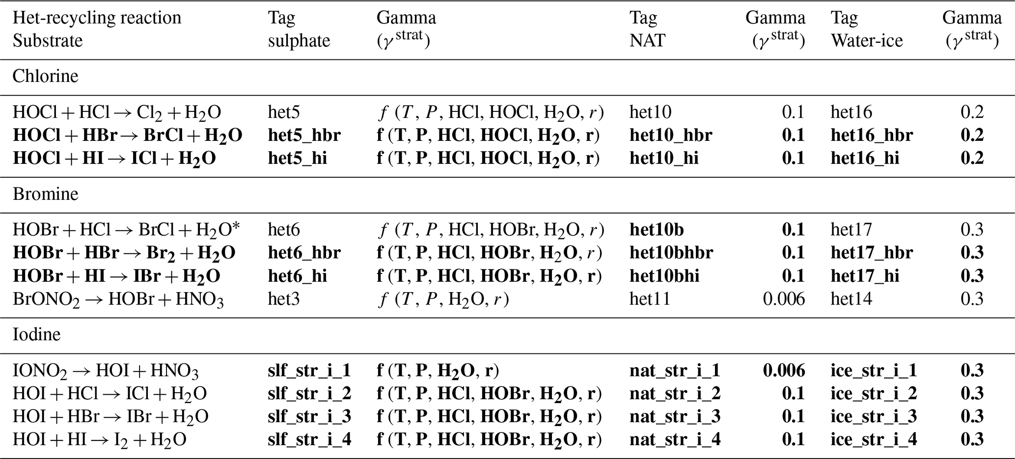
Bold font style highlights the mapped reactions and gammas applied to the corresponding regular font expression originally implemented in Marsh et al. (2013). For chlorine and bromine reactions we extended the original reaction tag-name, while for iodine expressions we adopted an independent tag-convention indicative of the substrate where each reaction occurs. ^* For the case of HOBr + HCl → BrCl + H₂O reaction only tag het10b was updated on top of the original scheme.

Implementation of stratospheric heterogeneous reactions of inorganic halogen reservoirs arising from the photodecomposition of long-lived halogens in WACCM are important for representing the ozone layer (Marsh et al., 2013). This includes temperature and water-vapour dependent re-activation reactions of chlorinated and brominated reservoirs occurring on stratospheric sulphate (SAD_sulfc), ice-crystals (SAD_ice) and nitric acid trihydrate (SAD_NAT) surfaces (Kinnison et al., 2007), including recent updates of individual stratospheric accommodation coefficients (γ^strat; Solomon et al., 2015). Based on Cuevas et al. (2022), in CESM2-SLH we extended WACCM developments to both low-top (32L) and high-top (70L) vertical configurations (see Sect. 3.1) by mapping equivalent heterogeneous reactions in the stratosphere for the minor halogenated reservoirs (mainly HOCl and HOBr), as well as the previously neglected iodine species (see Table 3). Here, we assumed identical accommodation coefficients and reaction yields for iodine as those used for the equivalent chlorinated and brominated reservoirs. This assumption represents a lower-limit of iodine impacts, as previous studies suggest that the reactive efficiencies of iodine species are larger than those for bromine and chlorine (Solomon et al., 1994; Koenig et al., 2020). Based on the original implementation in CESM1 (Fernandez et al., 2017; Saiz-Lopez et al., 2023), for low-top configurations (see Table 6) we imposed prescribed stratospheric sulphate aerosols above the tropopause (Mills et al., 2016), which results in smaller SAD_sulfc fields compared to those computed with MAM4 (see Fig. S4). Note that equivalent logical conditions based on mask${}_{\mathrm{ice}}^{\mathrm{strat}}$ have also been applied to all equivalent tropospheric reactions occurring over tropospheric ice-crystals to avoid double counting.

2.3 Species-specific dry and wet deposition

The implementation of species-independent dry and wet deposition processes in CESM1 CAM4-Chem has been previously described in the literature (Ordóñez et al., 2012; Fernandez et al., 2014; Saiz-Lopez et al., 2014). Here we briefly summarize the main approaches used to compute the removal or sink of SLH from the atmosphere, focusing on the few cases where a different approach was implemented in CESM2-SLH. Note that the model only considers the removal of inorganic halogen species, and therefore the sinks of VSL halocarbons are only chemical while for inorganic PGs deposition represents the major sink.

The depositional flux of gas-phase halogenated inorganic species due to dry deposition is calculated as the product of the deposition velocity of each individual species times its concentration at the lowest model surface (Lamarque et al., 2012; Ordóñez et al., 2012). Table 4 summarises the complete list of gas-phase species that are considered in the drydep_list, and shows the individual deposition velocity for each species. In addition, inorganic halogens are also removed by wet-deposition, following the default NEU scheme (Neu and Prather, 2012). Both nucleation scavenging (rainout) and impaction scavenging (below-cloud washout) are implemented in the wet-removal schemes based on Lamarque et al. (2012), although in CESM2-SLH we avoid mapping the ice-uptake of halogen species to that of HNO₃, as this resulted in too efficient washout of bromine and iodine in the upper troposphere (Fernandez et al., 2014). The individual Henry law constants (k_H) for all chlorine, bromine and iodine species shown in Table 4 are mostly based on the compilations from Sander (2015) and IUPAC (Atkinson et al., 2007, 2008).

Table 4 Independent halogen species considered for dry and wet deposition in CESM2-SLH.

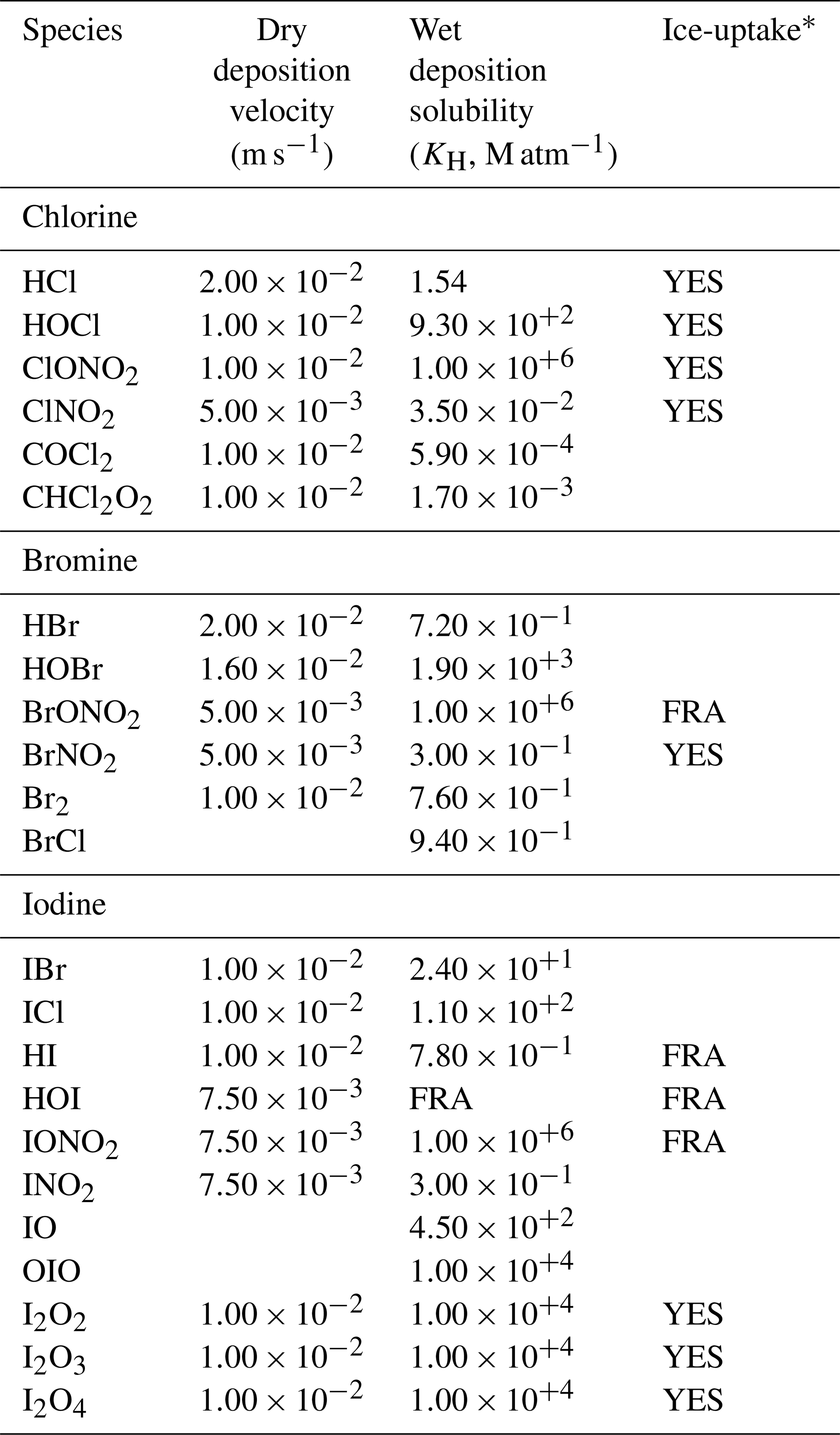
^* FRA indicate that for that particular case, the Free Regime Approximation was applied, see Table 5.

Halogenated reservoir species are assumed to be adsorbed by liquid droplets and ice-crystals, where they can undergo either: (i) reactive uptake (chemical recycling and re-emission back to the atmosphere) or (ii) permanent removal from the gas phase through washout (substrate capture/adsorption). Consequently, the modelled total inorganic halogen loading (Cl_y, Br_y and I_y), particularly in the Tropical Tropopause Layer (TTL), is determined by the competition between the wet deposition efficiency relative to the heterogeneous recycling (Aschmann et al., 2011; Aschmann and Sinnhuber, 2013). For iodine, Saiz-Lopez et al. (2014, 2015) determined that it was not possible to reproduce IO observations in the free troposphere because the NEU scheme washout of major iodine reservoirs was too efficient and iodine was completely removed within the lower troposphere. Therefore, for the particular case of HOI, HI and IONO₂, we calculate wet deposition with the FRA unimolecular approach for the dominant I_y species, considering Eq. (4a) to determine the collisional frequency. These ice-uptake processes are assumed to lead to deposition of iodine from the atmosphere (see non-stoichiometric removal reactions in Table 5). For HOI, which is the dominant iodine species in the lower troposphere, the FRA was implemented for both liquid-droplets and ice-crystals, where the former considers the surface area density of liquid clouds (SAD_liq) and the latter considers SAD_ice (Saiz-Lopez et al., 2014). Note that the non-reactive uptake or substrate capture of higher-order iodine oxides is also assumed to proceed efficiently on sea-salt aerosols following the FRA approach (Saiz-Lopez et al., 2015), although due to the efficient I_xO_y photolysis this additional sink of atmospheric iodine is a minor contributor compared to scavenging of major I_y species. We note that the ice-uptake for BrONO₂, one of the most abundant brominated reservoirs in the TTL and lower stratosphere, followed the NEU scheme and was assumed to be infinitely efficient in CESM1 (Fernandez et al., 2014). Following the FRA approach implemented for IONO₂, we have now implemented the FRA for BrONO₂ on ice-crystals in CESM2-SLH, which led to better agreement of the contribution of inorganic bromine to the total stratospheric bromine budget within tropical regions (see Sect. 4.2.1).

Table 5 Free Regime Approximation reactions representing a net sink of inorganic halogens in CESM2-SLH.

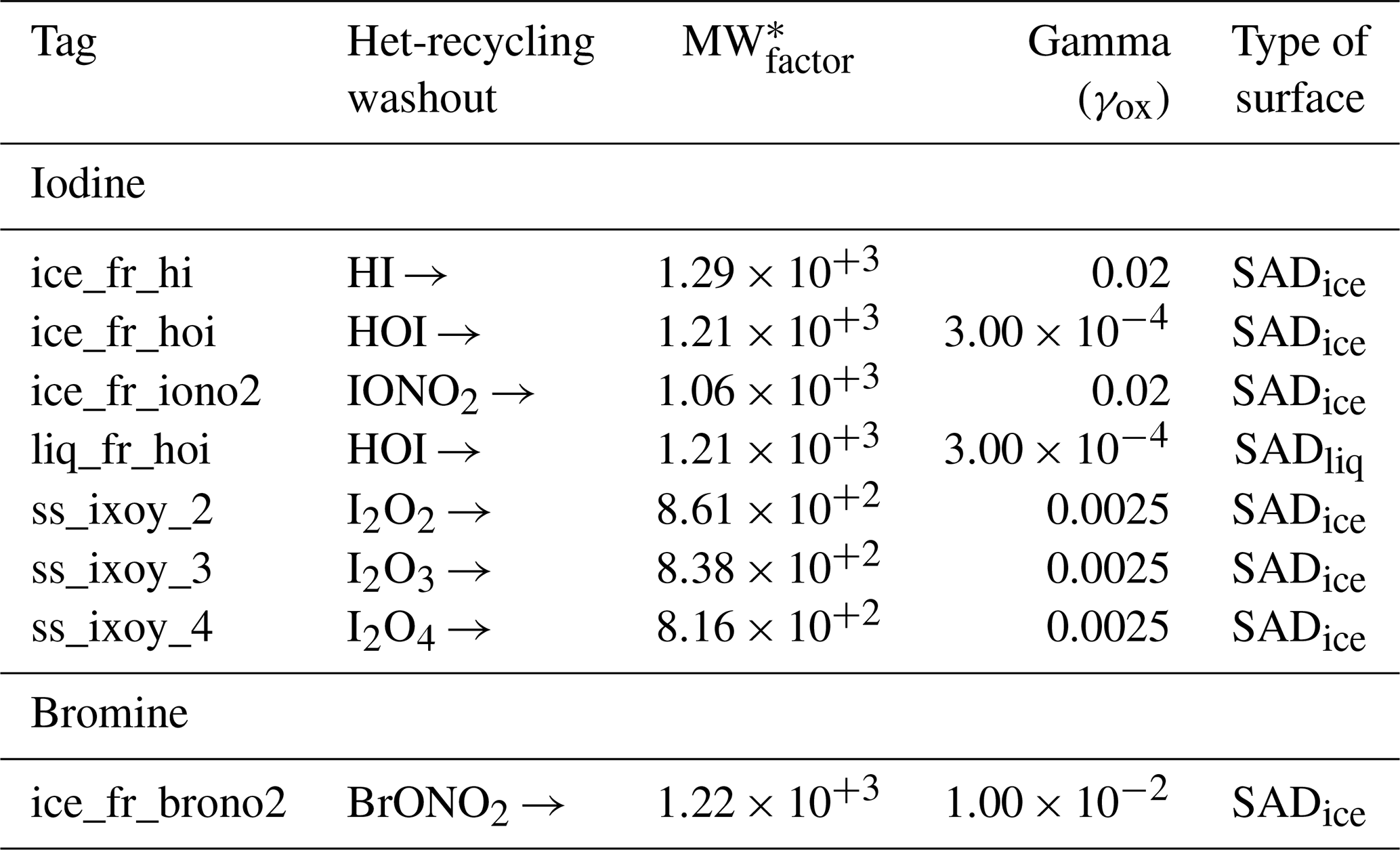
^* Values for the molecular weight factor (MW_factor) correspond to the following term from Eq. (3), $\left(\sqrt{\frac{\mathrm{8}\times R}{\mathit{\pi }\times {\mathrm{MW}}_{\mathrm{ox}}}}\right)$, where temperature has been excluded from the square-root and is later multiplied by an independent ($\sqrt{T}$) term.

3 CESM2-SLH release

The implementation of SLH sources and chemistry described in this work was performed over the base FCnudged and FCHIST atmospheric chemistry compsets (https://docs.cesm.ucar.edu/models/cesm2/config/2.2/compsets.html, last access: 4 May 2026). In CESM terminology, compset is an acronym for “component setup” and refers to specific model configuration of the Earth System Model, specifying which components are used and how they are coupled (Danabasoglu et al., 2020). These base chemistry compsets are forced with prescribed SSTs, while an additional fully-coupled chemistry-climate compset for WACCM has also been developed based on BWHIST (Gettelman et al., 2019b). Given the relevance for the computation of SLH sources and sinks, we highlight that prescribed CESM2-SLH compsets follow the climatological SST configuration from Huang et al. (2017) and an explicit representation of SSA lifting, transport and removal based on three individual bins (Tilmes et al., 2023). This differs from the original SSA representation available in the CAM4-Chem version used for the initial implementation of SLH in CESM1. Similarly, we note that the default dynamical core namelist options in CAM6-Chem (Davis et al., 2022) are based on the new nudging approach considering MERRA2 (Modern-Era Retrospective analysis for Research and Applications v2) reanalysis (Rienecker et al., 2011). This new nudging approach allows to select which physical variables (i.e., vertical and horizontal wind velocity, temperature, water vapour and/or pressure) are nudged, defining independent relaxation times for each, while previous CAM4-Chem configurations followed the old Specified Dynamics (SD) approach (Kunz et al., 2011) that forced identical relaxation times for all nudged magnitudes.

CESM2-SLH porting was performed on top of version 2.2.0 of CESM2 (Danabasoglu et al., 2020), particularly over branch cesm2.2-asdbranch, which includes CAM6 tagged version cam_cesm2_2_rel_09. Based on these versions, we forked and created the new CESM2-SLH and CAM6-SLH branches called cesm2.2-asdbranch_slh and cam_cesm2_2_rel_09_slh, respectively, which incorporate SLH updates within the main FORTRAN routines as well as modifications to building scripts (e.g., cime and cime_config) and default namelist variables (see Appendix). These open-access community developments allow to download, clone and build all SLH compsets available (see Code and Data Availability below; Fernandez et al., 2026a).

The representation of aerosols in general circulation models, including CESM, plays a key role for predicting halogen production via SSA-dehalogenation, which in turn impacts on the SLH tropospheric budget and burden. The major difference between CESM1 (CAM4-Chem) and CESM2 (CAM6-Chem) is that the former uses a continuous bulk representation of aerosols with four size bins, whereas the latter uses a modal representation with three bins (Danabasoglu et al., 2020). Another relevant difference is that MAM4 is the default dust scheme in CESM2 (Liu et al., 2016). Consequently, the vertical extent of SSA in the free-troposphere was largely reduced to improve the model overestimation obtained in previous studies (Lamarque et al., 2012; Tilmes et al., 2023). Therefore, to allow adjusting the online efficiency of the SSA-dehalogenation flux and avoid unrealistic changes in the atmospheric burden of tropospheric halogens due to parallel SSA developments, the released CESM2-SLH version now includes a group of SLH scaling factors (&slh_nl,) within the user-defined namelist (user_nl_cam). These tuneable scaling factors allow individual users to adjust the SSA-dehalogenation source in the different model resolutions and configurations in order to assure a consistent halogen atmospheric loading that are consistent with those shown in this work (see Sect. 5.3 and Appendix for further details).

Table 6 Summary of the different SLH compsets developed in CESM2-SLH.

3.1 Model compsets and resolutions

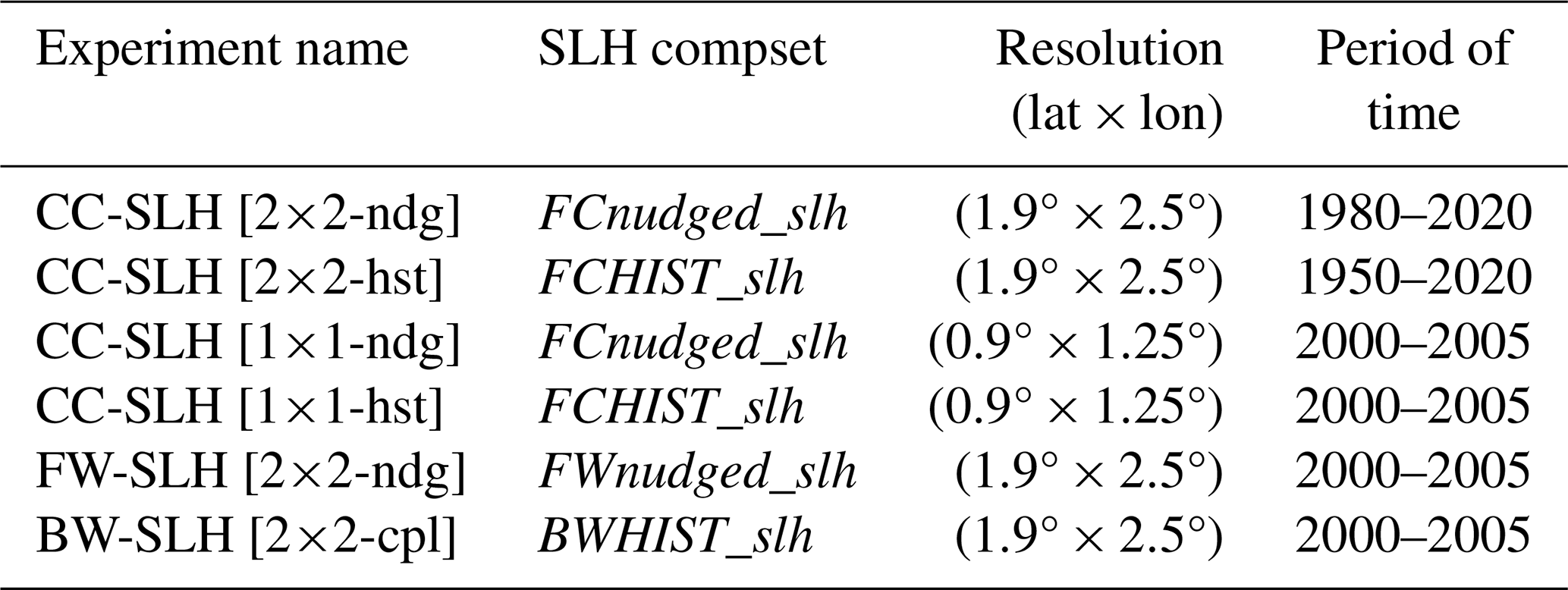
Two main CESM2-SLH configurations have been developed based on the available CAM6 base atmospheric chemistry compsets: FCHIST_slh and FCnudged_slh (see Table 6), where the former resolves atmospheric dynamics internally (free-running) and the latter is forced by prescribed meteorological fields (new nudging approach for specified dynamics). Both configurations employ the coarse f19_f19_mg17 horizontal resolution (1.9° latitude × 2.5° longitude, hereafter 2°×2°) and 32 vertical levels (low-top) from the surface to approximately 40 km (∼4 hPa). Unless stated otherwise, all external forcings and namelist options, including prescribed ocean SST and ice-coverage fields as well as solar radiation, cloud microphysics, gravity-wave dragging and dust emission factors are identical to those used in the base FCHIST and FCnudged configuration of CESM2 (Danabasoglu et al., 2020; Emmons et al., 2020). This includes surface LBCs of ODSs and greenhouse gases (GHGs) based on the Climate Model Intercomparison Project Phase 6 (CMIP6; Meinshausen et al., 2017), as well as anthropogenic and biomass burning pollutant emissions from the Community Emission Data System (CEDS; Van Marle et al., 2017; Hoesly et al., 2018) as described in Emmons et al. (2020). To extend model simulations beyond the historical period, we concatenated prescribed emission and LBC data from CMIP6 until year 2015 (Eyring et al., 2016) with future projections following the CMIP6 Shared Socio-economic Pathway 3.70 (SSP-370) scenario for the period 2016–2100 (Meinshausen et al., 2020; IPCC, 2022). We note that additional emission and LBC files for other configurations using different SSP scenarios are available in the published CESM2-SLH repository and can be changed through user-defined namelist options (see Appendix). In addition, equivalent model configurations using a finer resolution f09_f09_mg17 grid (0.9° latitude × 1.25° longitude, hereafter 1°×1°) have also been tested and adjusted to reproduce results obtained with the 2°×2° grids. In addition to the low-top configurations, whole atmosphere (high-top) fully-coupled BWHIST_slh (f19_g16) and FWnudged_slh (f19_f19_mg17) compsets were developed, both considering the coarse 2°×2° resolution and 70 vertical levels as their corresponding base atmospheric WACCM compsets. Table 6 summarizes the names and specifications of the main CESM2-SLH compsets.

3.2 Model experiments and sensitivity simulations

The complete set of model experiments performed in this work is presented in Table 7. Each experiment's name is composed by a prefix denoting the model used and the inclusion of short-lived halogens (e.g., CC-SLH for CAM6-Chem with SLH turned on) and a suffix indicating the model resolution and meteorology option (e.g., [2×2-ndg] for coarse resolution and nudging approach). Although all model configurations have been validated, initial results presented in Section 4 are mostly based on low-top and coarse CC-SLH [2×2-ndg] and/or CC-SLH [2×2-hst] experiments. We note that for each of the six SLH experiments listed in Table 7, an additional sensitivity was conducted neglecting the sources and chemistry of short-lived halogens (e.g., the corresponding CC-NOH [2×2-ndg] experiment, see Appendix). For most analysis comparing CC-SLH and CC-NOH distributions, we used the FCnudged_slh compset as this ensures that dynamical transport is consistently represented across experiments, which is crucial for isolating and quantifying chemical changes.

Table 7 CESM2-SLH experiments performed in this work.

In addition to the CESM2-SLH experiments presented above, and with the intention to validate current model performance compared with previous CESM1 studies, we also analysed model output from the main simulations originally published by Li et al. (2022) and Saiz-Lopez et al. (2023), as well as in Barrera et al. (2023) and Bossolasco et al. (2025). For consistency, these experiments are referred to, respectively, CESM1-SLH [QL22], CESM1-SLH [SL23], CESM1-SLH [JB23] and CESM1-SLH [AB25]. Although these CESM1 configurations are not strictly identical, the experiments were conducted considering analogous spatial resolution and nudging options to those employed here in CESM2-SLH. They are therefore considered as the benchmark simulations for quantitative and qualitative intercomparison between CESM model versions. Further details of the main similarities and differences between SLH results performed with CESM1 and CESM2 are described below.

3.3 SLH developments not implemented in CESM2

As described in Sect. 2, the initial implementation and the subsequent updates of SLH sources and chemistry in CESM1 were performed in consecutive studies focused on different regions of the atmosphere and/or different processes affecting each of the individual halogen families within the complete SLH scheme. Simultaneously, other non-SLH related model developments in different versions of CESM were also implemented, which have introduced variations in the distribution and impacts of SLH compared to the initial studies. Therefore, with the intention of: (i) including the most scientifically-validated representation of SLH influence on atmospheric composition in the latest released version of CESM; and (ii) keeping the closest model setup to the current CESM2 configurations commonly used for global climate and air quality studies; several SLH developments implemented in CESM1 have not been included in the released CESM2-SLH version. The reasons behind these exclusions and their potential implications for interpreting SLH impacts on atmospheric composition are detailed below:

• Emission-driven Methane simulations: although Li et al. (2022) highlighted the importance of performing emission-driven CH₄ simulations to properly evaluate the SLH influence on methane burden and radiative forcing, all default CESM2 configurations consider CH₄ LBCs altogether with other long-lived halogenated ODS and greenhouse gases (N₂O and CO₂). Consequently, current CESM2-SLH configuration does not allow evaluating direct (Cl-driven) and indirect (OH-driven) impacts of SLH chemistry on methane lifetime and radiative balance described by Li et al. (2022) and Saiz-Lopez et al. (2023). Nevertheless, an initial implementation of emission-driven CH₄ configuration in CESM2-SLH is presented in Mirrezaei et al. (2026).

• Continental Inorganic Halogen emissions: in addition to the anthropogenic halocarbon emissions of VSL chlorine, an anthropogenic emission inventory of continental inorganic halogens arising mostly from coal-burning and other sectors was developed in Saiz-Lopez et al. (2023). This inventory is mostly relevant for air quality studies focused on urban and/or continental regions (Chang et al., 2024; Fu et al., 2024), without contribution to the free troposphere and stratospheric halogen loading. Indeed, Saiz-Lopez et al. (2023) found that the SLH influence on global atmospheric composition and radiative balance is dominated by natural SLH emissions, whose source strength has been amplified by human activity since pre-industrial periods due to the efficient coupling of halogenated species with background air pollutants, e.g. the so called Anthropogenically Amplified Natural Emissions (AANE) sensitivity detailed in Saiz-Lopez et al. (2023).

• Polar sea-ice halogen sources and chemistry: given the substantial architectural code changes in many model components between CESM1 and CESM2 (Danabasoglu et al., 2020), the implementation of sea-ice halogen emissions and associated chemistry from polar regions (Fernandez et al., 2019, 2024) have not yet been fully tested and evaluated, particularly for the southern hemisphere. Consequently, these processes are not included in the current release of CESM2-SLH. This omission extends to other sea-ice related halocarbon emissions, such as those described by Abrahamsson et al. (2018).

• Halogen sources from dust: neither the photocatalytic chlorine production (van Herpen et al., 2023) nor the iodine release from dust (Koenig et al., 2021) have been implemented in the current CESM2-SLH release. We consider that further research is required before these complex heterogeneous redox processes can be robustly parameterized and included alongside the other widely validated SLH developments.

• Expanded sulphur chemistry scheme: this includes MeSH emissions and chemical processing reported by Wohl et al. (2024), as well as the hydroperoxymethyl thioformate (HPMTF) updated chemical scheme of DMS oxidation reported by Veres et al. (2020). Despite the important role played by SLH in the atmospheric sulfur cycle, these CESM1 additions are not directly related to SLH chemistry. Therefore, we have decided not to include them in the final CESM2-SLH release, maintaining the default CESM2 sulphur chemistry.

4 Results

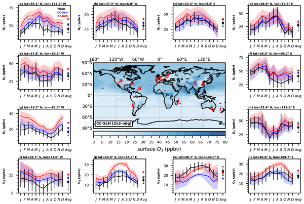
This section presents a comprehensive description of the main SLH effects on atmospheric composition obtained with the new CESM2-SLH model configuration, and is oriented to provide a general view for new users not familiarized with SLH chemistry. We focus on mean tropical, global, zonal and surface quantities, as well as their integrated values within the troposphere and stratosphere considering the model lapse rate tropopause. Results presented here show the net changes due to the SLH implementation, and, unless stated otherwise, are based on the difference between CC-SLH and CC-NOH experiments for the low-top (32L) and coarse (2°×2°) horizontal resolution. Section 4 is organized as follows: the individual emissions of organic and inorganic halogens are quantified in Sect. 4.1, altogether with the mean SLH surface and tropospheric burden changes across the historical (1980–2020) period. Section 4.2 evaluates the modelled spatio-temporal distribution of organic VSLS and inorganic halogens (reactive and reservoir species) during present-day conditions, defined as the mean 2015–2020 period. Section 4.3 assesses the impacts of SLH chemistry on the main atmospheric components during present-day, including O₃ and OH destruction, as well as the main changes in the chemical loss and production channels induced by SLH. Finally, Sect. 4.4 presents a comprehensive comparison between the different CESM2-SLH resolutions and configurations. Validation of the model performance is performed comparing CESM2-SLH simulations with multi-platform SLH observations in Sect. 4.2.1, as well as against surface ozone measurements over oceanic and coastal locations in Sect. 4.3.1.

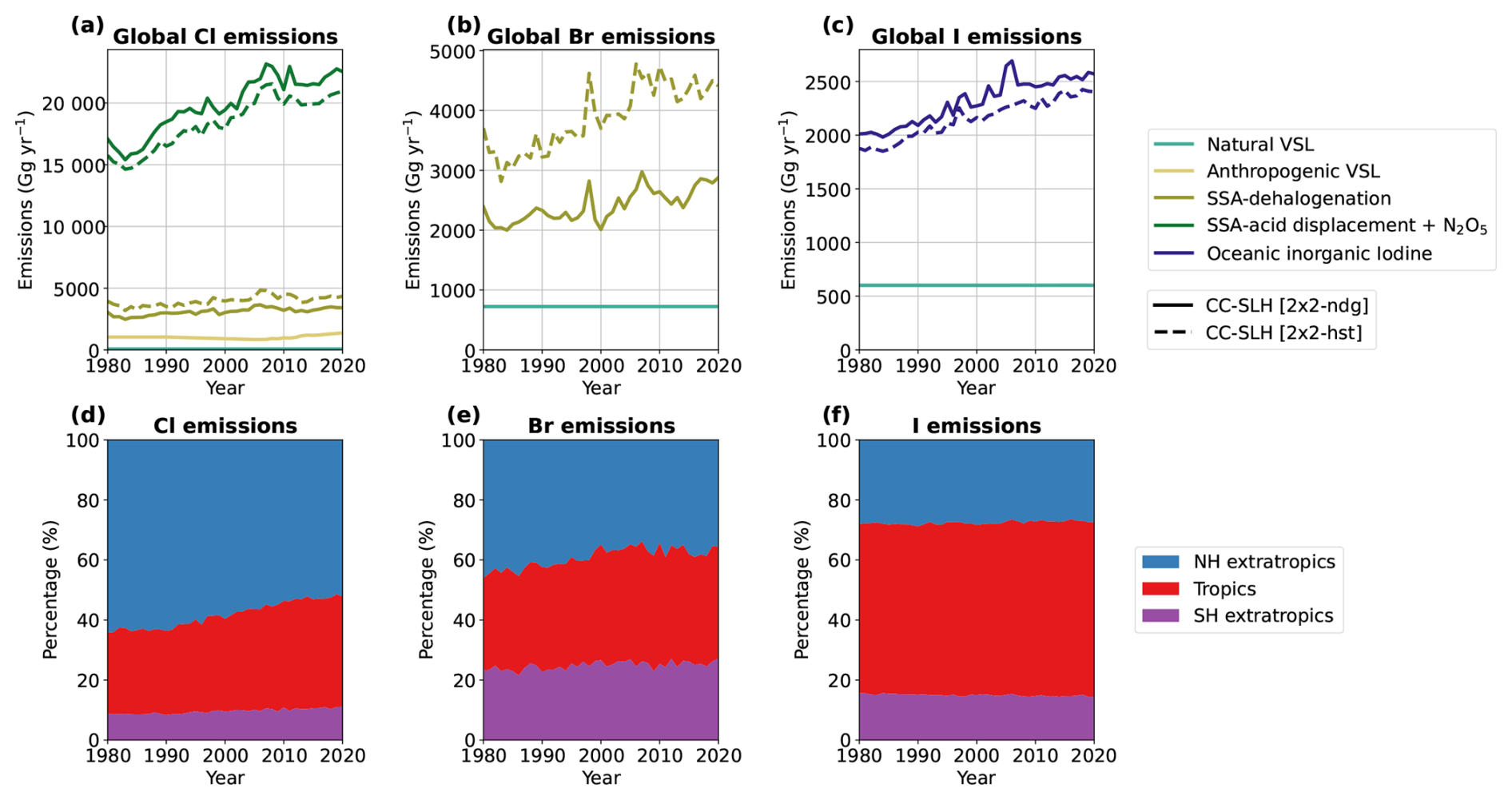
Figure 1 Historical evolution of global annual mean SLH emissions during 1980–2020. Top-row shows the individual contribution from offline and online sources for (a) chlorine, (b) bromine and (c) iodine, while bottom-row shows the percentage distribution within the Tropical (20° N–20° S) as well as Northern Hemisphere (NH = 20–90° N) and Southern Hemisphere (SH = 20–90° S) extra-tropical regions. Online emissions for the nudged CC-SLH [2×2-ndg] (solid) and free-running CC-SLH [2×2-hst] (dashed) experiments are distinguished, while the contribution from offline sources are equivalent for both simulations.

4.1 Evolution of SLH emissions and burdens during the historical period

Figure 1 shows the global mean evolution of SLH emissions from 1980 to 2020, as well as the hemispheric distribution of the total halogen sources discriminated for each individual halogen family. Note that the emission flux of natural oceanic VSL halocarbons remains constant throughout the entire period and constitutes the only source of natural bromo- and iodo-carbons (Fig. 1b and c). However, additional CH₂Cl₂ and C₂Cl₄ emissions from anthropogenic sources dominate the VSL chloro-carbon source (Fig. 1a). In all cases, we highlight that all emitted VSL halocarbons remain unreactive until they photolyze and/or are photochemically degraded by OH, where they release Cl, Br and I atoms that, due to their very high reactivity, react with other atmospheric components and partition among the different species within the Cl_y, Br_y and I_y halogen families (see Figs. 9 and 10). Although VSLS are not the primary source of halogens in the MBL, their photodecomposition constitutes the critical first step in releasing inorganic chlorine and bromine to the atmosphere. These initially released halogens can subsequently be amplified through non-stoichiometric heterogeneous recycling processes, particularly via SSA-dehalogenation.

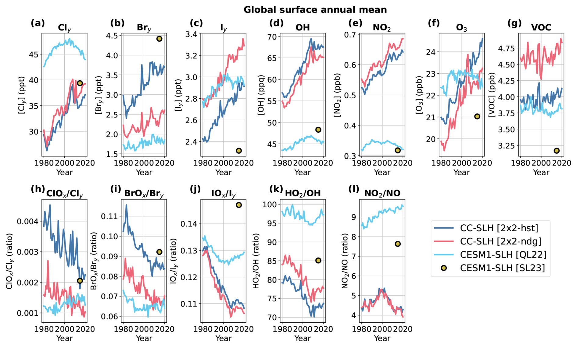
Figure 2 Historical evolution of global annual mean surface abundance and partitioning of main atmospheric components during 1980–2020. Top-row shows the total inorganic halogen surface abundance for (a) Cl_y, (b) Br_y and (c) I_y, as well as the surface mixing ratio for (d) OH, (e) NO₂, (f) O₃, and (g) VOC (calculated as the sum of species: ISOP, MTERP, CH₃OH, C₂H₅OH, CH₂O, CH₃CHO, CH₃COOH, CH₃COCH₃, HCOOH, C₂H₂, C₂H₄, C₂H₆, C₃H₈, C₃H₆, BIGALK, BIGENE, MEK, TOLUENE, BENZENE, XYLENES). Bottom row shows the reactive (XO_x) to reservoir (X_y) surface ratio (i.e., XO_x $/$ X_y) for (h) chlorine, (i) bromine and (j) iodine, as well as the (k) HO₂ $/$ OH and (l) NO₂ $/$ NO mean ratio at the model surface. Results for the nudged CC-SLH [2×2-ndg] (pink) and free-running CC-SLH [2×2-hst] (blue) experiments obtained with the CESM2-SLH release are compared with those obtained in previous CESM1 studies (see Sect. 3.3).

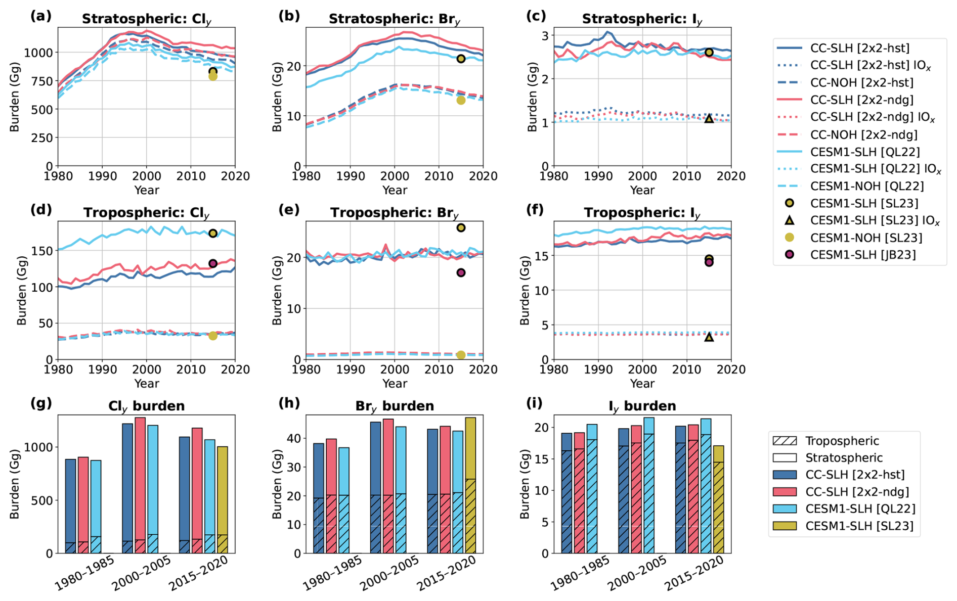
Figure 3 Historical evolution of global mean inorganic halogen burden during 1980–2020. Top-row shows the stratospheric burden for (a) Cl_y, (b) Br_y and (c) I_y, while middle-row shows the corresponding tropospheric burden for (d) Cl_y, (e) Br_y and (f) I_y for different model experiments including (CC-SLH, solid lines) and neglecting (CC-NOH, dashed lines) the contribution of SLH sources and chemistry. Given that the CC-NOH sensitivity does not consider iodine chemistry, panels (c) and (f) show the reactive iodine fraction (IO_x = I + IO) for CC-SLH experiment using dotted lines to avoid confusion with I_y. Results for the nudged CC-SLH [2×2-ndg] (pink) and free-running CC-SLH [2×2-hst] (blue) experiments are compared with those obtained in previous CESM1 studies (see Sect. 3.3). Bottom-row shows the mean total inorganic halogen burden for the 1980–1985, 2000–2005 and 2015–2020 periods using stacked columns distinguishing the tropospheric (striped) and stratospheric (empty unhatched) contributions for (g) chlorine, (h) bromine and (i) iodine.

In addition to offline VSL halocarbon emissions, inorganic halogen sources for chlorine, bromine and iodine are also computed online, which in all cases represent the dominant source of halogens to the atmosphere (Fig. 1 and Table 8). This online inorganic halogen flux shows an increasing emission trend between 1980 and 2020 (Fig. 1) for the three halogen families, although the main drivers of the parameterized expressions are significantly different for chlorine and bromine with respect to iodine (see Section 2.1.3). Indeed, Prados-Roman et al. (2015b) suggested that the online ocean–atmosphere coupling represents a negative geochemical feedback loop by which current ocean emissions of iodine (HOI + I₂) would be 2–3 times higher than in pre-industrial times, constituting a natural buffer for ozone pollution in the global marine environment. Results for both CC-SLH [2×2-ndg] and CC-SLH [2×2-hst] experiments show a global oceanic inorganic iodine flux increasing from 1.9–2.0 Tg I yr⁻¹ in 1980 to 2.4–2.5 Tg I yr⁻¹ in 2020 (Fig. 1c), with a dominant contribution from the tropical regions (Fig. 1f). In absolute terms, these values are larger than previously reported results obtained in CESM1, which ranged from 1.7–2.1 Tg I yr⁻¹ depending on the period of time and model configuration (Prados-Roman et al., 2015b; Iglesias-Suarez et al., 2020; Barrera et al., 2023; Saiz-Lopez et al., 2023). The larger iodine flux in CESM2-SLH is coherent with the higher CESM2 surface ozone abundances compared to CESM1 (Fig. 2f) (Emmons et al., 2020), which is the main driver of the oceanic iodine flux enhancement. However, we note that current CESM2-SLH oceanic iodine flux remain below other models that implemented iodine emissions (∼2.7 Tg yr⁻¹ in GEOS-Chem and ∼2.9 Tg yr⁻¹ in SOCOL; Sherwen et al., 2016b; Karagodin-Doyennel et al., 2021).

The online recycling emissions of chlorine and bromine are driven by, respectively, the acid-displacement reaction occurring on sea-salt aerosols and the SSA-dehalogenation source (Fig. 1a, b and Table 8). Similar to the oceanic inorganic iodine source, the modelled chlorine and bromine sources also increase from 1980 to 2020, although in this case the main driver is the positive trend in anthropogenic NO_x surface abundances (Fig. 2e). The net chlorine and bromine emissions respectively increase from approximately 15–16 Tg Cl yr⁻¹ and 2.0–3.0 Tg Br yr⁻¹ in 1980–1985 to 21–23 Tg Cl yr⁻¹and 2.8–4.4 Tg Br yr⁻¹ during 2015–2020. Here, we note that chlorine sources present a larger inter-hemispheric difference due to the dominant contribution of NO_x emissions in the Northern Hemisphere (NH) extratropical bands, which in turn increase the N₂O₅ and HNO₃ recycling (Fig. 1d). Following the larger SSA abundance within the CC-SLH [2×2-hst] (Fig. S2), the SAA-debromination source for this experiment is larger than that for CC-SLH [2×2-ndg], although the corresponding bromine sinks for the former is also larger than for the latter, resulting in equivalent bromine tropospheric burdens (see Table 8). Further details on the vertical distribution of individual emissions processes during present-day are provided in Sect. 4.2.

Figure 2 shows the inorganic halogen surface abundance during the 1980–2020 period for the CC-SLH [2×2-ndg] and CC-SLH [2×2-hst] experiments. In order to compare the current CESM2-SLH inorganic halogen abundances with previous studies, Fig. 2 also shows the results obtained in previous studies (i.e., CESM1-SLH [QL22] and CESM1-SLH [SL23] corresponding to Li et al., 2022 and Saiz-Lopez et al., 2023, respectively). These CESM1 configurations were selected as they allow for a better qualitative visualization and quantitative comparison of the absolute abundances of each halogen family and their reactive to inorganic halogen ratios (XO_x $/$ X_y, with XO_x = X + XO and X = Cl, Br and I), as well as the main atmospheric components driving the trends during the hindcast period. For example, given that the dominant halogen sources in the troposphere are computed online depending on the background concentration of NO₂ and O₃ (Fig. 2e and f), the surface abundance of Cl_y, Br_y and I_y (Fig. 2a–c) follows the temporal evolution of the former species within each model version. Indeed, the increasing trend in surface ozone abundance during the 1980–2020 period in CESM2-SLH compared to the more flatten trend observed in CESM1 (Fig. 2f) results in an increasing trend in iodine volume mixing ratios in the former, while I_y abundances in the latter remained approximately constant, particularly after year 2000 (Fig. 2c). A similar behaviour is also observed for Cl_y and Br_y, as their main sources depends mostly on the HNO₃ and N₂O₅ abundance as well as on the extent of partitioning of halogen reservoirs to ClONO₂ and BrONO₂, all of which increase for larger NO_x background conditions (Barrera et al., 2023). Compared with CESM1, the new benchmark tropospheric chemistry implemented in CESM2 includes updates in the oxidation of isoprene and terpenes, organic nitrate speciation, aromatic speciation and oxidation, as well as in the prescribed anthropogenic and biomass burning emission inventories, which in turn improves the representation of ozone and other secondary air-pollutants (Emmons et al., 2020). The total surface Br_y abundance for CC-SLH [2×2-hst] is larger than for CC-SLH [2×2-ndg] but both lie between previous CESM1 studies, while for the case of chlorine, both experiments are similar and show surface Cl_y abundances that are lower than in Li et al. (2022) and similar to Saiz-Lopez et al. (2023).

Figure 3 shows the tropospheric, stratospheric and total halogen burden across the 1980–2020 period for the CC-SLH [2×2-ndg] and CC-SLH [2×2-hst] experiments (solid lines) along with the corresponding CC-NOH [2×2-ndg] and CC-NOH [2×2-hst] (dashed lines) experiments. Equivalent comparisons for CESM1 are also shown. Several distinctive features are of major relevance to support the final CESM2-SLH configuration, as described below:

• Temporal evoluition of stratospheric halogen burden: the predicted trend shows a maximum peak just before and after year 2000 for chlorine and bromine, respectively, which is in line with the temporal variation of the dominant long-lived ODSs that dominate the inorganic halogen burden in the stratosphere (WMO, 2018, 2022). In both cases, the increase in stratospheric Cl_y and Br_y burden due to SLH are equivalent between CESM1 and CESM2 configurations. For stratospheric iodine, all experiments show an equivalent stratospheric burden that remains constant with time (see Sect. 4.2.1). Reaching an equivalent stratospheric halogen enhancement for all configurations provides confidence that the modelled influence of SLH in the lower stratosphere within CESM2-SLH are in line with previous studies.

• Global mean tropospheric halogen burden: the spread between the different CESM2-SLH experiments is smaller than that obtained with CESM1 in previous studies. Indeed, for the case of bromine, the tropospheric Br_y burden for both CC-SLH [2×2-ndg] and CC-SLH [2×2-hst] are equivalent to those obtained for CESM1-SLH [QL22], although they lie in between CESM1-SLH [SL23] and CESM1-SLH [JB23] (Fig. 3e). This range of tropospheric Br_y burdens arise due to changes in the seasonal and latitudinal sea-salt aerosol masks used when the CESM1 polar module is enabled (Fernandez et al., 2014, 2021), highlighting the large sensitivity of the SSA-dehalogenation source to the modelled changes in SSA abundance and distribution (see Fig. S2). The tropospheric Cl_y burden for both CESM2-SLH nudged and free-running configurations are equivalent to those obtained for CESM1-SLH [JB23] and lower than for CESM1-SLH [QL22] and CESM1-SLH [SL23] (Fig. 3d).

• Partitioning between reactive and reservoir species: Although the tropospheric Iy trend for all transient simulations follows the oceanic iodine flux increase due to the enhanced ozone levels between 1980 and 2020 (Fig. 2f), the overall stratospheric burden remains constant with time (Fig. 3c). This implies that most of the inorganic iodine enhancement occurring in the MBL and close to the surface is washed out in the free troposphere before reaching the tropopause. The larger present-day tropospheric I_y burden between CESM2-SLH experiments (17.2–17.7 Tg I) compared to CESM1-SLH [SL23] and CESM1-SLH [JB23] (14–14.5 Tg I) are explained by the significant changes in reactive (IO_x) vs. reservoir iodine partitioning (IO_x/I_y) between CESM1 and CESM2. Despite these differences in I_y burdens, the tropospheric IO_x burden for all CESM1 and CESM2 experiments are equivalent (see dotted lines in Fig. 3f), and therefore the influence of iodine on atmospheric composition shown in Sect. 4.3.3 remains consistent with previous CESM1 studies.

4.2 SLH abundance during present-day

Annual mean tropospheric halogen abundances, LBCs, sources and sinks during present-day (2015–2020) are summarized in Table 8. These global-mean reference values for the CC-SLH [2×2-ndg] and CC-SLH [2×2-hst] experiments should be taken as a guideline for any other CESM2-SLH configuration. The main similarities and differences between the recommended setup with respect to the remaining CESM2-SLH compsets and/or resolutions available (Tables 6 and 7) are described in Sect. 4.4.

The global annual emission flux for VSL halogens in CESM2-SLH during present-day is 65.3 Gg Cl yr⁻¹, 721.3 Gg Br yr⁻¹, and 599.7 Gg I yr⁻¹. Due to changes in transport and background OH abundance between CESM1 and CESM2 (see Fig. 2), we increased the flux strength of the original VSL inventory (Ordóñez et al., 2012) by 15 % for all VSL bromo- and chloro-carbons (e.g., CH₂Br₂ and CH₂BrCl) but retained the magnitudes of iodo-carbon species, including CH₂ICl and CH₂IBr. As a result, chlorinated (VSL_Cl) and brominated (VSL_Br) halocarbon emissions are, respectively, ∼6 % and 14 % larger in CESM2 compared to CESM1. VSL_Br shows a higher percentage change than VSL_Cl since the mixed iodocarbon species plays a smaller role in the overall VSLS flux in the case of bromine (CH₂IBr) compared to CH₂ICl for chlorine (Ordóñez et al., 2012). We highlight that the contribution of anthropogenic VSLS (1265.5 Gg Cl yr⁻¹) has also been increased by 15 % and results in surface fluxes up to 20 times larger than the natural oceanic source from VSL chlorocarbons (65.3 Gg Cl yr⁻¹). Here, it should be noted that the additional contribution from other anthropogenic VSL chlorocarbons (CHCl₃ and C₂H₄Cl₂) are also included as LBCs instead of considering offline emissions, reaching a total of ∼48 pptv at the lowest model level above the surface.

Table 8 Quantitative values for global annual SLH burdens during present-day (2015–2020) conditions.

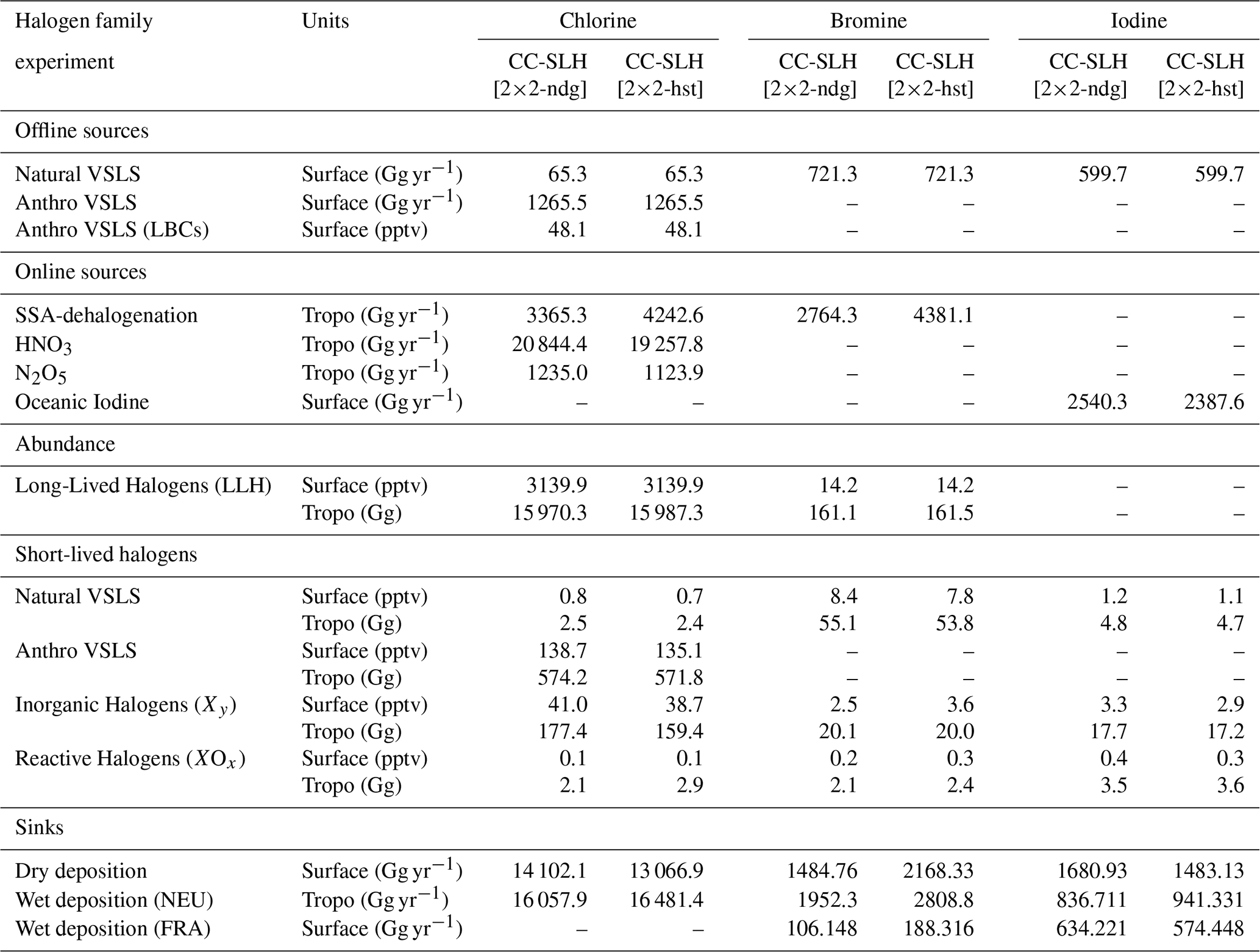
The largest variability among all online emissions arises from the uptake and release of bromine and chlorine from sea-salt aerosol. In absolute terms, the global annual mean SSA-dehalogenation source for CC-SLH [2×2-hst] is 877.3 Gg Cl yr⁻¹ (2 %) and 1616.7 Gg Br yr⁻¹ (58 %) larger than for CC-SLH [2×2-ndg] (see Table 8). This is explained by the non-linear response of Cl₂, Br₂ and BrCl sources resulting from the online computation of non-stoichiometric heterogeneous reactions described in Table 1 that enhance chlorine (bromine) emissions due to the iterative accumulation of gas-phase HOCl, ClONO₂ and ClNO₂ (HOBr, BrONO₂ and BrNO₂). As detailed in Sect. 2.1.3, this efficient recycling mechanism depends on the parameterized fields of SAD_SSA (Fig. S2) and the partitioning shift between different inorganic halogen reservoirs (Sect. 4.2.2). Similarly, the chlorine source from the acid-displacement for the CC-SLH [2×2-ndg] experiment is larger by ∼1700 Gg Cl yr⁻¹, which in relative terms represents only ∼8 % variability but in absolute terms surpasses the total contribution from VSL chlorine sources. We note that our present-day global chlorine source from acid displacement is equivalent to CESM1 (21.5 Tg Cl yr⁻¹) and around 4 times smaller than an equivalent implementation of acid displacement dehalogenation in TOMCAT (∼ 90 Tg Cl yr⁻¹; Hossaini et al., 2016). Similarly, the SSA-dehalogenation source in CESM2-SLH is between 1.5 and 3 times lower than the range of values estimated by Graedel and Keene (1995) (∼37–73 Tg Cl yr⁻¹) and less than half of the recent predictions from Wang et al. (2019, 2021) (∼50–64 Tg Cl yr⁻¹). For the case of bromine, our global annual flux of SSA-dehalogenation (∼ 2.8–4.4 Tg Br yr⁻¹) remains lower than other estimates obtained with GEOS-Chem when the reactivity of bromine with tropospheric aerosols is considered (3.5–6.4 Tg Br yr⁻¹; Chen et al., 2018; Zhu et al., 2019), and between 4 to 7 times smaller than their most recent predictions (∼20 Tg Br yr⁻¹; Wang et al., 2019, 2021).

Regardless of the large variability on the online computation of inorganic halogen sources, we highlight that CESM2-SLH considers a species-independent removal of inorganic halogens from the atmosphere, and consequently, the larger the emission flux for any specific configuration, the larger the corresponding global sink. Indeed, absolute and percentage changes in both dry and wet deposition between CC-SLH [2×2-ndg] and CC-SLH [2×2-hst] are of equivalent magnitude to their corresponding sources (Table 8). Here, it should be noted that the surface dry deposition occurring only at the model surface accounts for almost half of the total halogen sink, representing ∼ 45 %, ∼ 40 % and ∼ 50 % for chlorine, bromine and iodine, respectively. For the case of wet deposition tendencies, the NEU scheme represents the largest individual sink for bromine and chlorine, while for iodine, the NEU scheme accounts only for approximately half of the total wet deposition, with a substantial contribution from the FRA removal of HOI in liquid clouds. In contrast, the FRA only represents a small fraction (<5 %–7 %) of the total bromine wet deposition compared to the NEU scheme, as only ice-uptake of BrONO₂ is considered to occur through FRA (see Table 4). It is worth noting that although dry and wet deposition are computed for individual species, the net sink of each halogen family is typically dominated by a single or a couple of species that dominates the halogen partitioning in different layers of the troposphere (e.g., HCl for chlorine, HOBr and HBr for bromine and HOI for iodine, see Fernandez et al., 2014 and Saiz-Lopez et al., 2014).

Table 8 also quantifies the mean surface abundance and global tropospheric burdens for both organic VSLS and inorganic SLH during present-day. Differences between experiments in general remain below ∼10 %, with slightly larger halogen surface abundance and tropospheric burden for CC-SLH [2×2-ndg]. The exception is surface Br_y, which is ∼44 % larger in CC-SLH [2×2-hst] due to its larger SSA-dehalogenation source. However, note that the tropospheric Br_y burden between both experiments is almost identical (20.1 Gg Br for CC-SLH [2×2-ndg] vs. 20.0 Gg Br for CC-SLH [2×2-hst]). Surface chlorine abundance is dominated by anthropogenic VSLS reaching 135–139 pptv that largely surpass the natural contribution from the ocean (less than 1 pptv), while surface inorganic Cl_y reaches approximately 40 pptv. The corresponding values for brominated compounds reach 7.8–8.4 pptv for VSL bromine and 2.5–3.6 pptv Br_y, while for the case of iodine global mean values are 1.1–1.2 pptv and 2.9–3.3 pptv, respectively. Regarding the partitioning between reactive and reservoir halogen species for the different compsets, our model results show that surface and tropospheric XO_x $/$ X_y ratio for chlorine, bromine and iodine ranges between 0.2 %–1.8 %, 8 %–12 % and 10 %–21 %, respectively, with general larger values for CC-SLH [2×2-hst] compared to CC-SLH [2×2-ndg].

In contrast to bromine and chlorine, surface I_y abundance in CC-SLH [2×2-ndg] is ∼40 % higher compared to CESM1-SLH [SL23] (2.3 pptv I_y), which is mainly due to the different IO_x $/$ I_y and HO₂ $/$ OH ratios between the different nudging approaches among CESM versions (see Fig. 2j and k). However, free-running experiments (CC-SLH [2×2-hst] and CESM1-SLH [QL22]) show equivalent surface abundances, particularly for the 2015–2020 period. The larger OH abundance and lower HO₂/OH ratio in CESM2-SLH compared to CESM1 increases the contribution of HOI to the total I_y loading, and therefore, there is a major shift on the partitioning from reactive to reservoir species for iodine (see Table 8). Therefore, the reactive IO_x tropospheric burden in CESM2 (3.5–3.6 Gg I) is only ∼10% larger than the 3.2 Gg I estimated value found in Saiz-Lopez et al. (2023). Most notably, the spread in global I_y abundance between free-running and nudging CESM2 compsets is smaller than the spread in CESM1.

The contribution of inorganic chlorine, bromine and iodine to the total (tropospheric + stratospheric) burden when SLH are considered is shown in Fig. 3g–i. We found that for present-day conditions, the contribution of tropospheric Cl_y, Br_y and I_y to the total halogen loading represents ∼14 %, ∼47 % and ∼87 %, respectively. This increasing contribution of tropospheric X_y content going from chlorine to bromine to iodine is in line with the enhanced efficiency of each halogen species in reacting with tropospheric ozone (X + O₃ → XO + O₂, see Reaction R2), and results in tropospheric iodine to be the dominant species affecting the tropospheric oxidative capacity and ozone abundance (see Sect. 4.3.2). Given the turnover in stratospheric halogen loading from anthropogenic ODSs around year 2000, we note that the percentage contributions change for the different time periods.

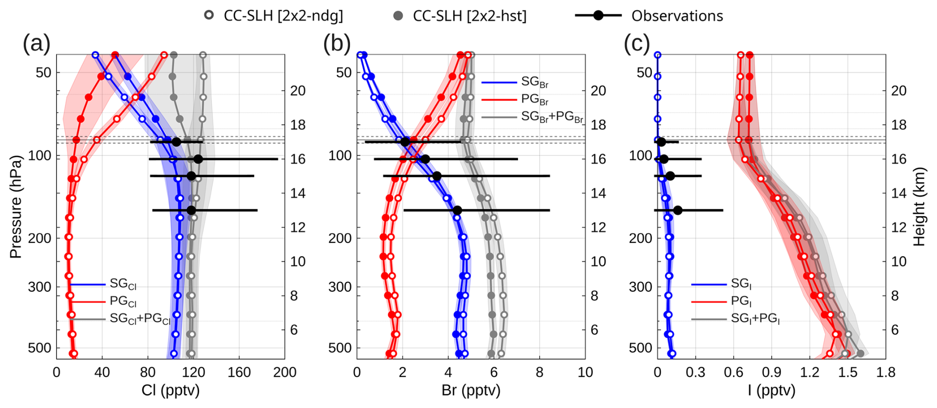
Figure 4 Tropical mean vertical profile of organic SLH source gases (SG_X) and product gases (PG_X) during present-day (2015–2020) for (a) chlorine, (b) bromine and (c) iodine. The SGs profiles (blue lines) correspond to the nudged CC-SLH [2×2-ndg] (empty symbols) and the free-running CC-SLH [2×2-hst] (filled symbols) experiments, while PGs profiles (red lines) are obtained as the difference with respect to the corresponding CC-NOH sensitivity (see text for details). The total additional halogen abundance due to SLH (SG_X + PG_X) is shown in grey. The tropical (20° N–20° S) mean and spread (i.e., ± the interannual standard deviation for the 2015–2020 period) are shown with solid lines and coloured shading, respectively. Average and range of observed VSLS mixing ratios in the tropical tropopause layer compiled in Tables 1–5 of WMO (2022) are shown in black symbols and solid-thick horizontal lines at 13, 15, 16 and 17 km, respectively. The solid and dashed horizontal lines indicate the tropical mean tropopause height ± standard deviation.

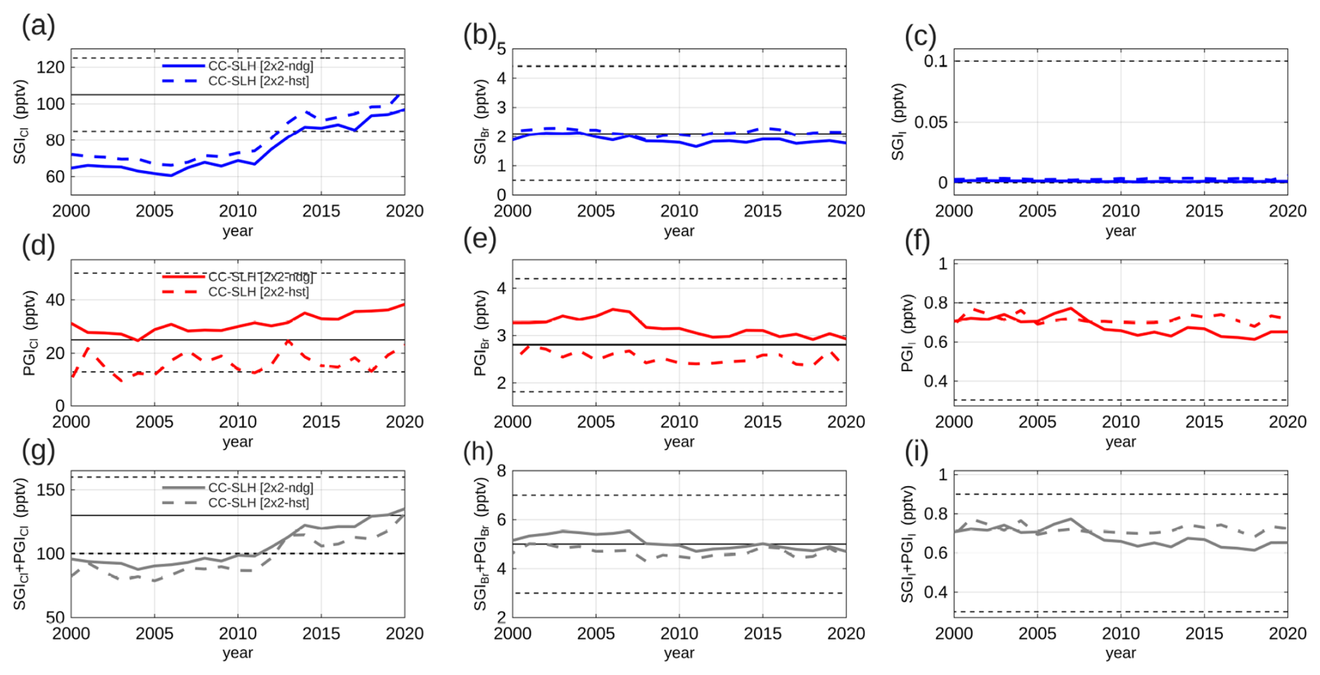
Figure 5 Temporal evolution of tropical (20° N–20° S) source gas injection (SGI_X, a–c), product gas injection (PGI_X, d–f) and total SLH injection (SGI_X + PGI_X, g–i) to the stratosphere from 2000 to 2020 for the nudged CC-SLH [2×2-ndg] (solid lines) and free-running CC-SLH [2×2-hst] (dashed lines) experiments. Individual results for (a, d, g) chlorine, (b, e, h) bromine and (c, f, i) iodine are respectively shown on the left, middle and right columns, respectively. The reported best estimate and range of SGI and PGI for each individual family compiled in Tables 1–6 of WMO (2022) are respectively represented by horizontal solid and dashed lines on each panel. Intermediate species COCl₂, CHCl₂O₂ and COFCl (see Fig. S3) are assumed to contribute to PGI_Cl.

4.2.1 Validation of SLH abundance with observations

Several studies highlight the importance of properly distinguishing between the contribution of Source Gas Injection (SGI) and Product Gas Injection (PGI) to the stratosphere when representing the contribution of SLH to stratospheric ozone depletion (Fernandez et al., 2014, 2021; Salawitch et al., 2005; WMO, 2018, 2022). This is mainly because the ozone destruction efficiency of SLH in the lowermost stratosphere depends on the net fraction of the emitted VSLS that has already been converted to the reactive inorganic form (Fernandez et al., 2021). Figure 4 shows the tropical mean (20° N–20° S) vertical profiles of all VSL source gases (SG_X) along with the associated increment of inorganic product gases (PG_X). Since the simulations neglecting SLH have non zero Cl_y and Br_y abundance, the PG_Cl and PG_Br vertical profiles were computed as ΔCl_y and ΔBr_y, respectively (i.e., the difference between the CC-SLH and CC-NOH experiments). Therefore, PG_Cl and PG_Br exclusively account for the additional contribution of SLH to the total inorganic halogen loading at any given height, without considering the small (but not negligible) contribution from long-lived chlorine and bromine photodecomposition close to the tropopause (see Fig. 10a and c). In addition, Fig. 4 shows the sum of all organic and inorganic species for each halogen family (SG_X + PG_X).

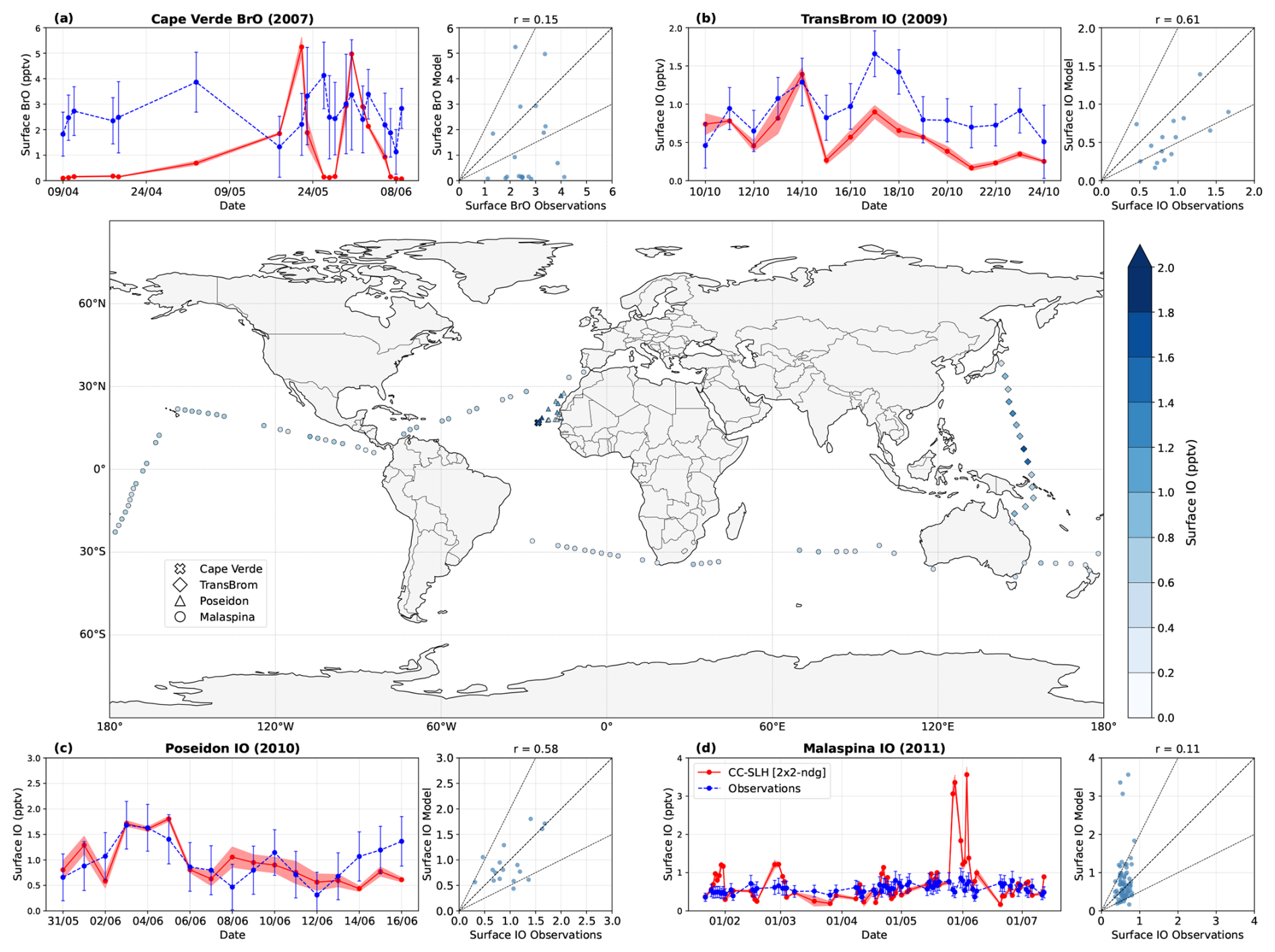
Figure 6 Comparison of IO and BrO surface mixing ratios between nudged CC-SLH [2×2-ndg] and observations. The central panel shows the location of a coastal surface station where BrO was measured as well as the routes of three ship-based IO campaigns (coloured markers). Side panels show time series of observations (blue dashed line with reported root-mean square error (RMSE) bars) and model outputs (red line with ± 1 standard deviation), along with modelled vs. observed scatterplots with correlation coefficients (r). Measurement campaigns are (a) Cape Verde; (b) TransBrom; (c) Poseidon and (d) Malaspina. All data corresponds to daytime conditions.

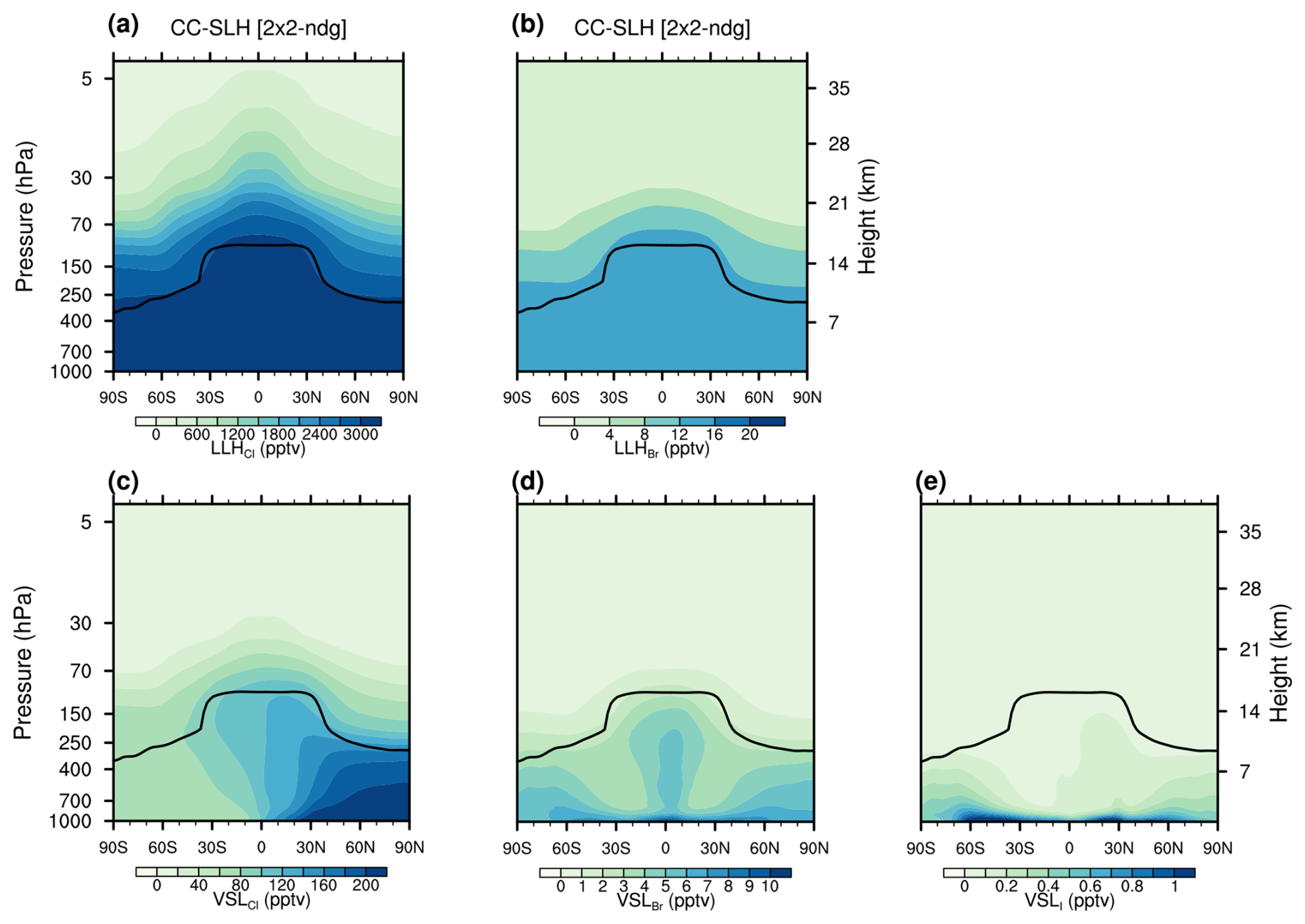
Figure 7 Zonal average distribution of the organic halogen fraction during present-day (2015–2020) for the nudged CC-SLH [2×2-ndg] experiments. Top row shows the long-lived (LLH) distribution for (a) chlorine (LLH_Cl) and (b) bromine (LLH_Br). Note that CESM2-SLH does not include long-lived iodine species. Bottom row shows the very short-lived (VSL) distribution for (c) chlorine (VSL_Cl), (d) bromine (VSL_Br) and (e) iodine (VSL_I). The black solid line shows the mean model tropopause.

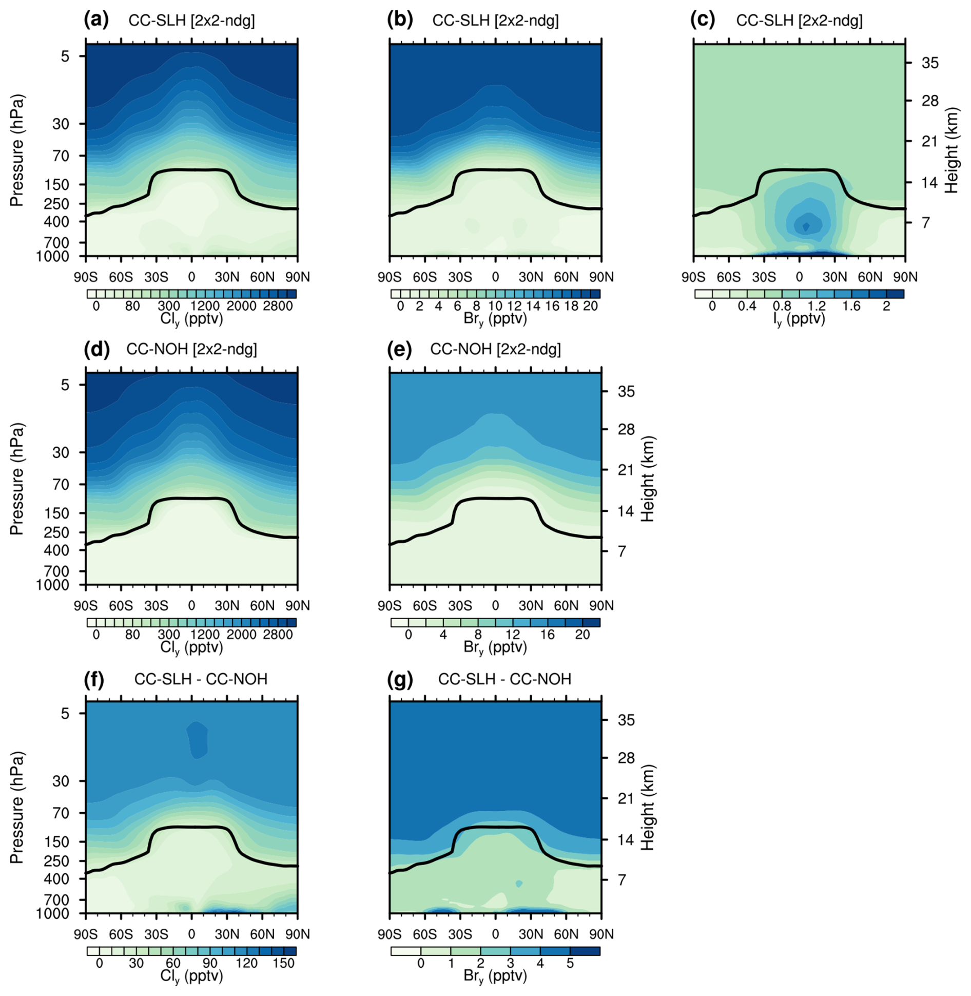
Figure 8 Zonal average distribution of total inorganic halogen (X_y) during present-day (2015–2020) for different nudged model experiments including (CC-SLH [2×2-ndg]; a–c) and neglecting (CC-NOH [2×2-ndg]; d, e) the contribution of SLH sources and chemistry. The bottom-row (f, g) shows the absolute difference between both simulations (CC-SLH–CC-NOH). Left column (a, d, f) shows the distribution for chlorine (Cl_y), while the middle (b, e, g) and right (c) columns show the distribution of bromine (Br_y) and iodine (I_y), respectively. The black solid line shows the mean model tropopause. Note that CC-NOH [2×2-ndg] sensitivity does not consider iodine chemistry.

Stratospheric injection is computed at approximately 85 hPa (17 km) within the tropics, just above the mean model tropopause. At this level, the simulated contribution of SGI and PGI to the total bromine injection reaches 1.8–2.2 pptv + 2.5–3.0 = 4.3–5.2 pptv during present-day (Fig. 4b). Notably, all experiments simulate SGs vertical profiles that fall within the accepted range reported in the last Ozone Assessment Report (WMO, 2022) throughout the tropical troposphere, regardless of the compset and resolution considered. Indeed, our simulations show a continuous conversion of SGs to PGs just below the tropopause that results in a larger fraction of inorganic bromine injection (PGI) relative to the organic halocarbon fraction (SGI). Once all organic VSL_Br has been converted into reactive Br_y, the total contribution of SLH to the stratospheric bromine loading remains nearly constant at ∼5 pptv roughly from the tropopause to the model top (grey line in Fig. 4b). Here we note that the dominant contribution of VSLS to the total SGI arises from the major CH₂Br₂ and CHBr₃ emissions, with only minor contributions from the remaining VSL bromocarbons (Fernandez et al., 2014). In contrast, CH₂IBr emissions, which constitute the largest source of VSL bromine mass to the atmosphere (Ordóñez et al., 2012), barely contributes with a negligible fraction to the stratospheric SGI due to its particularly short lifetime. Unlike bromine, the larger lifetime of chlorinated VSLS imply that the total chlorine injection (114–126 pptv) is dominated by SGI (91–97 pptv), with a smaller contribution from PGI (17–35 pptv), in agreement with reported ranges (WMO, 2022). For the case of iodine, much faster photochemistry compared to chlorine and bromine implies that almost the complete injection occurs through PGI = I_y (Fig. 4c), with a total injection of approximately 0.65–0.72 pptv, in agreement with observations and previous estimations using CESM1 (Saiz-Lopez et al., 2015; Koenig et al., 2020).

Figure 5 shows the temporal evolution of SGI_X and PGI_X occurring at the model tropical tropopause for chlorine, bromine and iodine for the CC-SLH [2×2-ndg] and CC-SLH [2×2-hst] experiments, where the modelled values are compared with the latest assessed values of SLH injection to the stratosphere (i.e., see Tables 1–6 in WMO, 2022). The modelled contribution of SLH to PGI for all three halogens does not show a significant trend and lies within the WMO estimates across the simulated period. For the particular case of bromine and chlorine, CC-SLH [2×2-ndg] shows slightly larger values than the CC-SLH [2×2-hst], coherent with the different representation of tropical convective transport and Brewer-Dobson circulation between nudged and free-running experiments. Modelled SGI_Cl shows a growing trend across 2000–2020 in agreement with previous reports (Hossaini et al., 2019) approaching the assessed 2019 atmospheric abundance by the end of the simulated period (WMO, 2022). Here we recall that in CESM2-SLH we applied the same 15 % enhancement to natural oceanic bromine sources as well as to anthropogenic chlorine emissions and LBCs. In quantitative terms, SLH contributes to a significant enhancement on present-day stratospheric bromine loading of approximately 25 %–26 % compared to other long-lived halogen (LLH) sources, while for chlorine, the contribution of SLH represents only an increase of 3.7 %–3.8 %, in agreement with the latest estimation from WMO (2022). The iodine SGI contribution is almost zero and all the iodine injection to the stratosphere occurs as PGI (Fig. 5c).

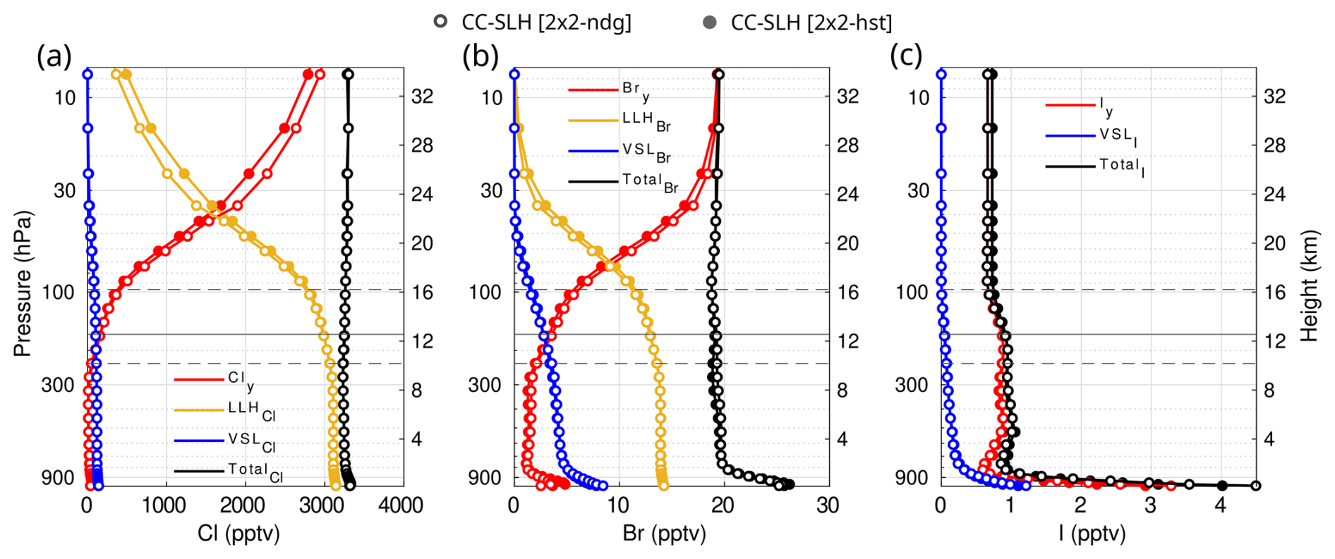
Figure 9 Global mean vertical profile of organic and inorganic halogens during present-day (2015–2020) for (a) chlorine, (b) bromine and (c) iodine. Each coloured line shows individual contributions from organic long-lived (LLH_X, yellow). very short-lived (VSL_X, blue) and total inorganic (X_y, red) halogens, together with the sum of all contributions (Total_X, black) for each species (X = Cl, Br, I) for the nudged CC-SLH [2×2-ndg] (empty symbols) and free-running CC-SLH [2×2-hst] (filled symbols) experiments. Solid and dashed horizontal lines indicate the global mean tropopause height ± standard deviation.

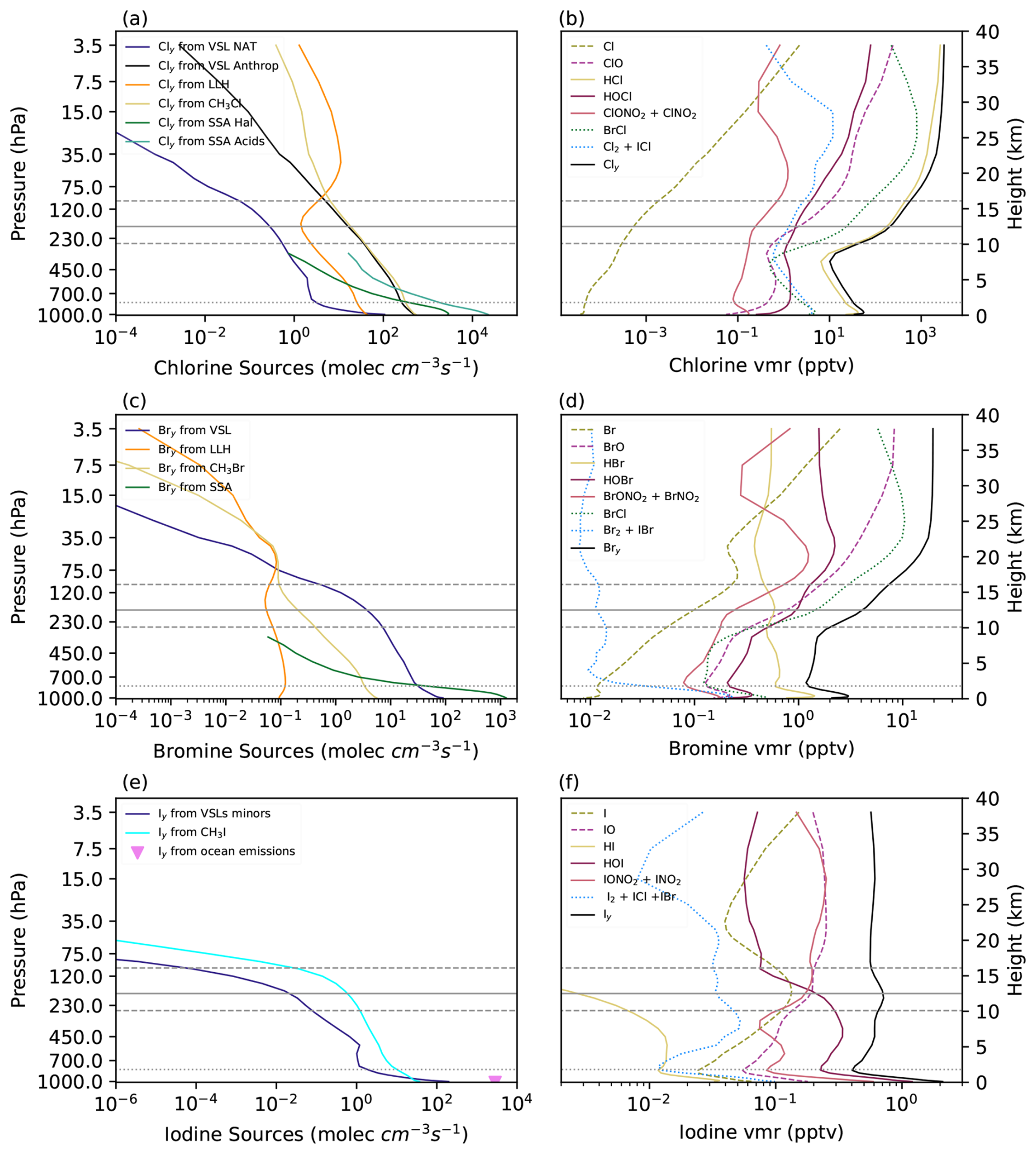
Figure 10 Global mean vertical profile of inorganic halogen release from different types of sources (a, c, e) and the corresponding abundance for the different species conforming each halogen family (b, d, f) during present-day (2015–2020). Individual panel show results for (a, b) chlorine, (c, d) bromine and (e, f) iodine for the CC-SLH [2×2-ndg] experiment. The halogen atom release arising from the photochemical (OH + hν) degradation of organic very short-lived (VSL, blue) and long-lived (LLH, yellow) halogens, including the independent contribution from CH₃Cl and CH₃Br (orange) are distinguished on the left panels. The vertically-resolved inorganic halogen source arising from SSA-dehalogenation and acid-displacement processes is shown in greenish colours, while the surface oceanic iodine emission is indicated by a pink triangle. Right panels show the contribution of each individual halogen species to the total inorganic halogen loading (X_y, black), where dashed lines highlight the abundance of the dominant reactive halogen species (X and XO) for each family (X = Cl, Br, I). The horizontal solid and dashed lines show the global mean tropopause height ± standard deviation, while the horizontal dotted line corresponds to P=850 hPa.

Additional model validation was performed extracting hourly surface reactive halogens mixing ratios for the CC-SLH [2×2-ndg] experiment at the same location and time as previously published observations obtained in multiple measurement campaigns. Three ship-based campaigns measured IO concentrations: TransBrom, conducted in October 2009 from Japan to Australia (Großmann et al., 2013), Poseidon, which surveyed the coasts of Northwest Africa between the Canary Islands and Cape Verde in June 2010 (Bange, 2011) and Malaspina, conducted between January and July 2011, which circumnavigated the globe from Brazil to Spain via Australia and the Panama Canal (Prados-Roman et al., 2015a). Additionally, we compared measurements from a coastal station in Cape Verde between April and June 2007 (Read et al., 2008; Mahajan et al., 2010). The ship routes and the location of Cape Verde are shown in the central panel of Fig. 6. The side panels compare daily mean modelled (red) and observed (blue) values, where the shading and error bars represents the modelled spread and the reported observational uncertainty, respectively. A general good agreement is achieved, especially for IO where observed values ranging between 0.5 and 2 pptv with a sharp variability that can exceed 1 pptv between consecutive days is captured in magnitude by the model, although not always for the exact time and location. The maximum values predicted in Malaspina during late May and early June (Fig. 6d) are attributed to highly localized IO bursts due to the large partitioning shift between I_y species driven by SSA recycling (Prados-Roman et al., 2015a). Similarly, near-zero BrO values are modelled in Cape Verde (Fig. 6a) due to the negligible contribution of SSA-debromification predicted by the model during early April. However, during late May the model is capable of reproducing the magnitude of sporadic BrO peaks due to the improved representation of SSA abundance over the east-Atlantic. Despite the remaining model-observation discrepancies, we highlight that CESM2-SLH results in a general underestimation of observed reactive halogen abundance, which implies that the predicted influence of SLH on atmospheric composition is, in any case, a lower limit.

4.2.2 Latitudinal and vertical distribution of SLH

Figure 7 shows the zonal average latitudinal-height distribution of total organic long-lived (Fig. 7a and b) and short-lived (Fig. 7c–e) halogens for the CC-SLH [2×2-ndg] experiment during present-day. While long-lived halogenated ODSs remain unreactive throughout the troposphere and are converted to inorganic Cl_y and Br_y only after crossing the tropopause, VSL halocarbons photolyze at much lower heights in the atmosphere. Consequently, iodine VSL is nearly completely decomposed in the lower troposphere (Fig. 7e), whereas only a small fraction of the emitted VSL bromine and chlorine SGs is transported unaltered to the stratosphere (Fig. 7c and d). In contrast to the naturally emitted bromine and iodine VSLS, the modelled VSL chlorine abundances show a remarkable inter-hemispheric difference with larger values over the NH, due to its dominant anthropogenic sources (Fig. 7c).

In addition, Fig. 8 shows the corresponding zonal average distribution of inorganic halogens (Cl_y, Br_y and I_y) from the model surface up to the middle stratosphere for CC-SLH [2×2-ndg] (Fig. 8a–c) and CC-NOH [2×2-ndg] (Fig. 8d and e), as well as the difference between both experiments (Fig. 8f and g). Note that CC-SLH [2×2-ndg] does not consider any long-lived iodine source (Fig. 7) while CC-NOH [2×2-ndg] does not include iodine chemistry at all (Fig. 8). Notably, not only the total X_y abundance at the model top, but also the conversion from organic SGs to inorganic PGs occurs at lower heights for CC-SLH [2×2-ndg] (Fig. 8a and b) than for CC-NOH [2×2-ndg] (Fig. 8d and e), following the different ODS and VSLS photodecomposition shown in Fig. 7. Given the typically longer photochemical lifetimes of long-lived chlorinated compounds compared to brominated halons (see Table A1 in the Annex of WMO, 2022), the latter presents a steeper vertical gradient in the lower stratosphere and an almost complete conversion to inorganic bromine in the upper stratosphere (Fig. 9b).

The change in inorganic halogen abundance X_y due to SLH (Fig. 8f and g) highlights the different behaviour for each individual halogen family in different regions of the atmosphere. For example, within the troposphere, both Cl_y and Br_y show a pronounced enhancement in the MBL and close to the surface mostly in the NH mid-latitude regions that is rapidly reduced in the free-troposphere, which is driven by the efficient SSA-dehalogenation source and acid displacement that presents a sharp vertical profile (see green lines in Fig. 10a and c). For the case of iodine, the largest abundances at the surface are driven by the strong HOI/I₂ emission occurring in the tropical regions (Fig. 1f). In this region, up to 1 pptv of I_y is transported to the tropical free troposphere where, due the local changes in ozone abundance and temperature, a pronounced partitioning shift lead to the formation of the tropical rings of atomic halogens (Saiz-Lopez and Fernandez, 2016). A fraction of this tropospheric inorganic iodine is washed out, and the remaining fraction is injected to the stratosphere as inorganic PGs through the tropical tropopause region with an almost negligible contribution from SGs (see Fig. 4). In contrast, Fig. 8f shows a gradual enhancement in Cl_y occurs in the middle stratosphere, which arises due to the longer photochemical lifetime of chlorinated VSLS which are mostly transported unaltered to the lower stratosphere (Fig. 4a). For bromine, Figs. 7d and 8g highlight that both organic SGs and inorganic Br_y PGs contribute to the total stratospheric bromine loading due to SLH.

Figure 9 summarizes the global mean (90° N–90° S) vertical profiles of the sum of all organic and inorganic halogen species from the Earth's surface to the middle stratosphere for the CC-SLH [2×2-ndg] and CC-SLH [2×2-hst] experiments. The figure distinguishes the contributions from long-lived chlorine and bromine species, as well as the total halogen fraction transported as VSL SGs and inorganic PGs, consistent with Figs. 7 and 8. The conversion of unreactive organic SGs to reactive PGs is found to be very similar between the two meteorological representations (free-running vs. nudged dynamics) among model compsets. We note that these global and annual mean averages lumped together continental and oceanic domains within the boundary layer, as well as tropospheric and stratospheric parcels due to the latitudinal variation of the tropopause (see dashed horizontal lines in Fig. 9). However, three main differences characterizing the vertical distribution for each halogen family are distinguished. First, the tropospheric chlorine abundance is dominated by long-lived species, with minor contributions from VSL chlorine and Cl_y. Due to the long lifetimes of CFCs and CH₃Cl, the crossing point between LLH_Cl and Cl_y representing the photochemical conversion from the organic to the inorganic fractions occurs in the middle stratosphere (∼ 40 hPa, see Fig. 9a). Second, the VSL bromine contribution is comparable (although smaller) to the contribution from long-lived halons and CH₃Br, and therefore the initial enhancement in Br_y abundance, as well as the crossing point with LLH_Br, occurs at lower heights in the stratosphere (∼ 75 hPa, Fig. 9b). Third, given that there are no long-lived iodine species and the short photochemical lifetimes of VSL_I (particularly CH₃I), both the tropospheric and stratospheric abundance is dominated by inorganic I_y. This is in line with the tropospheric and stratospheric mean burdens shown in the stacked bars of Fig. 3g–i.

Given that the atmospheric impact of SLH over different atmospheric components depend on the overall abundance of reactive halogens, whose initial step is the release of a halogen atom through Reactions R1a and b, left panels in Fig. 10 shows the Cl, Br and I atom release from the different organic and inorganic sources as a function of height. Here note that only emissions or processes that lead to net inorganic halogen production are considered. In addition, right panels in Fig. 10 show the chemical partitioning between all halogen species constituting each inorganic halogen family (X_y) which interconvert between one and the other following gas-phase and heterogeneous phase reactions involving other atmospheric components such as O₃, OH and NO₂ (see summarized Reactions R1–R13 scheme in Sect. 1 and Tables S1–S3).

As summarized in Table 8, SSA-dehalogenation is the dominant source of bromine and the second largest source for chlorine. However, Fig. 10a and c highlights that these sources are primarily confined to the lower troposphere where most of the washout takes place. For chlorine, the contribution of the acid-displacement HCl release dominates, increasing surface Cl_y particularly in the NH mid-latitudes and coastal locations (Fig. 11d). The photochemical degradation of both VSL_Cl and VSL_Br dominates the release of Br and Cl atoms throughout the free troposphere, although the biogenic ocean flux is the sole source of bromine, while for the case of chlorine the contribution from anthropogenic VSL_Cl is at least two orders of magnitude larger than the natural oceanic source. In addition, the release of Cl atoms from long-lived CH₃Cl accounts for an equivalent source as that arising from anthropogenic VSL_Cl (Fig. 10a). In contrast, bromine release from long-lived CH₃Br only surpass that arising from VSL_Br in the stratosphere (Fig. 10c). For iodine, ocean HOI/I₂ release dominates the surface emissions, while the photochemical degradation of CH₃I alone controls the organic to inorganic iodine conversion throughout the troposphere (Fig. 10e).

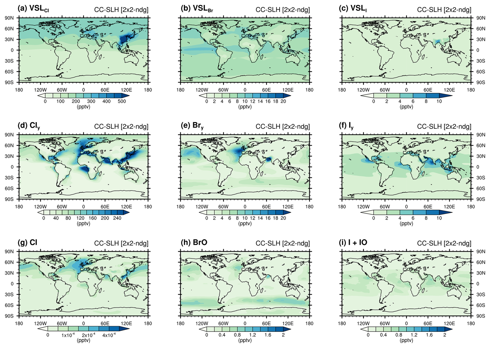
Figure 11 Annual mean geographical distribution of organic and inorganic halogens during present-day (2015–2020) for the CC-SLH [2×2-ndg] experiment. Top row shows the very short-lived (VSL) distribution for (a) chlorine (VSL_Cl), (b) bromine (VSL_Br) and (c) iodine (VSL_I), while middle-row shows the distribution of the total inorganic halogen content for (d) chlorine (Cl_y), (e) bromine (Br_y) and (f) iodine (I_y). The bottom-row shows the corresponding distribution for the most important reactive halogen species for each family: (g) Cl atom, (h) bromine monoxide (BrO) and (i) reactive iodine (IO_x = I + IO). All magnitudes have been averaged from the model surface up to 850 hPa.

Figure 10b shows that the dominant inorganic chlorine species throughout the troposphere is HCl, which represents between 63 % and 85 % of the total Cl_y partitioning. The Cl atom and ClO partitioning are generally 4 and 1 to 2 orders of magnitude smaller than the global mean Cl_y, respectively, although due to rapid heterogeneous recycling their contributions on the regional scale can increase, particularly in coastal locations (see Fig. 11). For bromine (Fig. 10d), the dominant species in the lower troposphere is HBr both during day and night (Fernandez et al., 2014). However, during reactive transport to the upper troposphere, HBr is heterogeneously converted on ice-crystals first to HOBr and finally to the dominant BrONO₂ fraction in the stratosphere (see Tables 2 and 4). The vertical profile of iodine partitioning in Fig. 10f shows that HOI is the dominant iodine species throughout the troposphere and therefore its washout controls the transport and abundance of inorganic iodine from their dominant surface sources to the stratosphere. It should be noted that the chemical partitioning from reservoir to reactive halogen species is the largest for iodine, followed by bromine and last by chlorine (i.e., IO_x/I_y > BrO_x/Br_y > ClO_x/Cl_y). This is associated with the much faster photochemistry of iodine compared to bromine and, to a larger extent, chlorine, which in turn controls the efficiency of each halogen family in altering the composition and oxidative capacity of the troposphere (see Sect. 4.3.2).

4.2.3 Geographical heterogeneity and seasonality of SLH

Figure 11 shows the spatial distribution of carbon-bonded VSLS (Fig. 11a–c), total inorganic halogens (Fig. 11d–f) and the most relevant reactive fraction (Fig. 11g–i) of each halogen family averaged over model levels with P≥850 hPa and for the time period 2015–2020. Note that depending on the halogen family considered, the most relevant reactive species for each family are shown: i.e., Cl atom for chlorine, BrO for bromine and the sum of I + IO = IO_x for iodine.

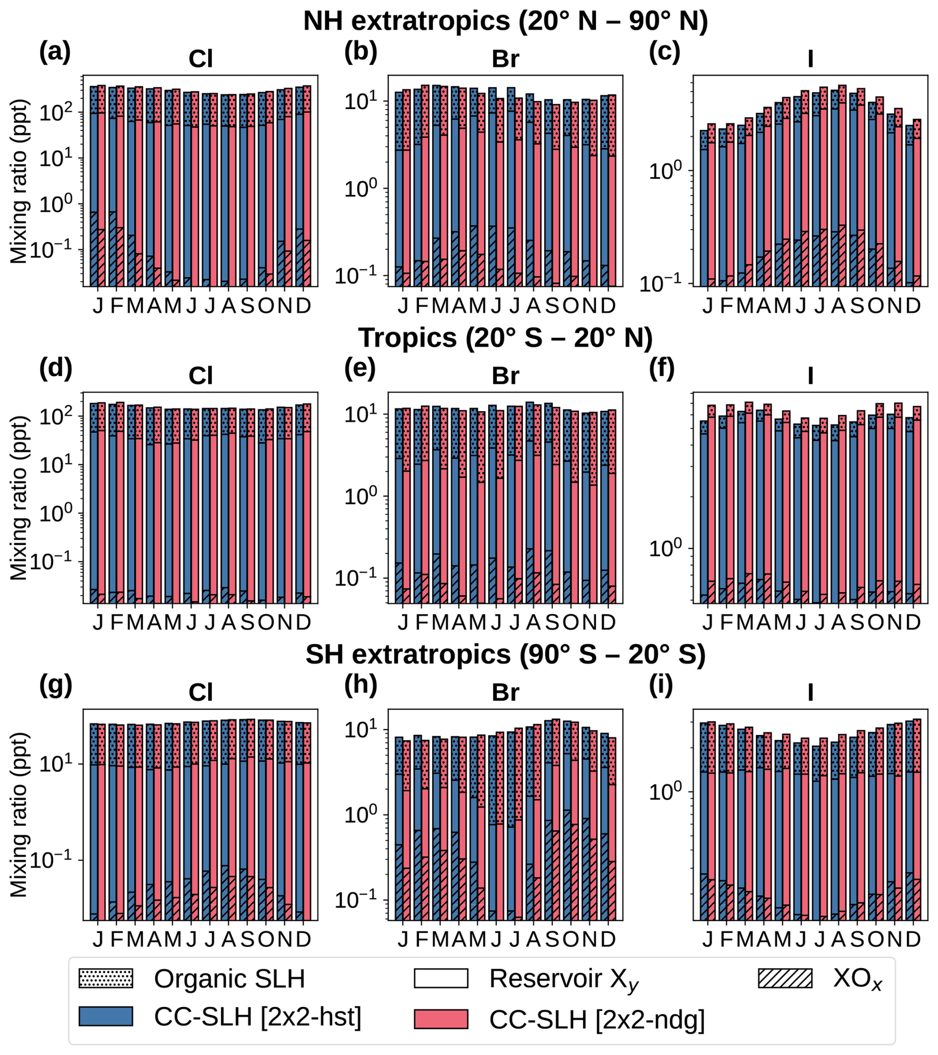
Figure 12 Seasonal distribution of total SLH abundance during present-day (2015–2020) for (a–c) Northern Hemisphere (NH = 20–90° N) extratropics; (d–(f) tropical (20° N–20° S) mean; and (g–i) Southern Hemisphere (SH = 20–90° S) extratropics. Each coloured stacked bar distinguishes the contribution from organic VSL_X (stippled bars), reactive (XO_x, striped bars) and reservoir (empty unhatched bars) halogens (i.e., the sum of reactive XO_x plus reservoir species representing total inorganic halogens, X_y) for the nudged CC-SLH [2×2-ndg] and free-running CC-SLH [2×2-hst] experiments.

Driven by the prevalence of anthropogenic sources in the NH, VSL_Cl exhibits a pronounced South–North latitudinal gradient between ∼60 and ∼260 pptv (Fig. 11a), with peak values exceeding 500 pptv over China. In contrast, VSL_Br shows a more homogeneous spatial distribution with maximum abundances observed over the equatorial regions due to the dominant source from the tropical oceans (Ordóñez et al., 2012). Minimum, maximum and mean global VSL_Br mixing ratios reach 2.9, 12.9 and 6.8 pptv, respectively. The global mean VSL_I is ∼1.0–1.2 pptv (see Table 8). Inorganic chlorine also maximizes over the NH, particularly over coastal locations where the mixing of halogen-rich SSA and HNO₃/N₂O₅ plumes results in an enhanced chlorine source. The highest Cl atom concentrations occur over the coastal regions of Europe, US and East Asia, with maximum values smaller than $\mathrm{0.4}\times {\mathrm{10}}^{-\mathrm{3}}$ pptv and a global mean average of $\mathrm{4}\times {\mathrm{10}}^{-\mathrm{5}}$ pptv. These distributions are consistent with maximum and mean Cl_y levels of ∼640 pptv and ∼47 pptv, respectively (Fig. 11d). Similarly, modelled Br_y also maximizes over coastal regions co-located with high SSA abundance (Fig. S2). However, the inter-hemispheric bromine enhancement is less pronounced than for chlorine because SSA-debromination is not controlled by HNO₃ and N₂O₅, but instead by shifts in Br_y partitioning between BrONO₂, BrNO₂ and HOBr (see Table 1). Maximum Br_y peaks in the NH are up to 2 times larger than in the Southern Hemisphere (SH). However, the corresponding maximum BrO abundances does not present such inter-hemispheric asymmetry (Fig. 11h), highlighting the strong dependence of reactive bromine partitioning on the background atmospheric composition of NO_x and HO_x. For iodine, global I_y distributions is primarily controlled by oceanic HOI/I₂ emissions that peak within the tropics. The mean modelled I_y and I + IO surface abundances reach ∼1.25 pptv and ∼ 0.15 pptv, respectively, with corresponding volume mixing ratios spanning between (0.05–21) pptv for I_y and (0.008–0.90) pptv for I + IO. Notably, the global mean IO_x $/$ I_y ratio is ∼0.12, whereas in regions with the highest I_y, abundances it remains below ∼0.04.

Table 9 Quantitative changes in atmospheric composition between CC-SLH and CC-NOH experiments.

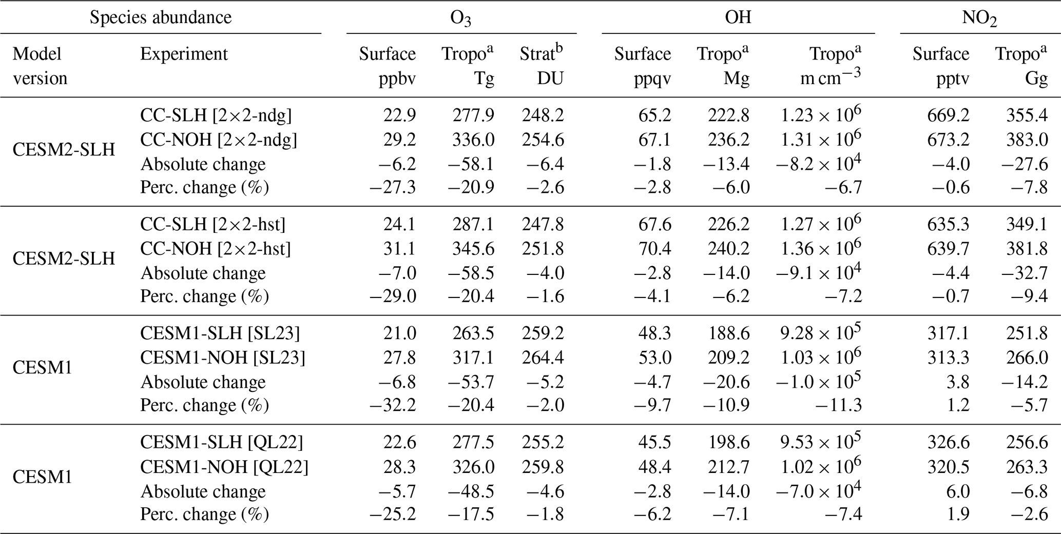
^a Tropospheric magnitudes express the total mass and have been computed considering the chemical tropopause (O₃ < 150 ppbv). For the case of OH, the global mean tropospheric abundance in molec. cm⁻³ is also shown. ^b The stratospheric ozone column is expressed in Dobson Units (DU) and computed for O₃ ≥ 150 ppbv. Equivalent CC-SLH–CC-NOH differences are obtained regardless of considering the chemical or lapse rate definition for the tropopause.

Figure 12 presents the seasonal variation of surface organic and inorganic halogen species averaged within different latitudinal bands, distinguishing between the tropics (20° N–20° S) and the extratropical domains in the NH (20–90° N) and the SH (20–90° S). The stacked bars shown in Fig. 12 represent the total halogen abundance decomposed into the reactive (XO_x) and reservoir species, as well as organic VSL_X species for each experiment. The corresponding zonal average seasonality of VSL_X halocarbons, as well as the geographical X_y (reactive plus reservoir) seasonal cycle over the boundary layer are shown in Figs. S5 and S6, respectively. We first describe the seasonality in the NH extratropics and then highlight the main similarities and differences with the SH extratropics and the tropical mean.

The NH extratropical Cl_y presents a pronounced seasonal cycle with approximately doubled values during the boreal winter (∼90–100 pptv) compared to the summertime (∼45–50 pptv). This is coherent with the seasonal variation of the heterogeneous recycling efficiency that reduces the conversion of both chlorinated (e.g., ClONO₂) and nitrogen (e.g., N₂O₅ and HNO₃) reservoirs to more reactive species. For the same reason, the organic VSL_Cl and VSL_Br abundances also peak during the winter when the photochemical decomposition is smallest (see Fig. S5). In contrast, the iodine seasonal cycle shows maximum abundances during the summertime, both for I_y and VSL_I. This is explained by the dominant contribution of oceanic sources for iodine, which increase associated with the larger fraction of ice-free ocean in summer. The inorganic Br_y abundance is lower and maximizes during the spring for CC-SLH [2×2-ndg] in comparison with CC-SLH [2×2-hst], which shows larger values and a maximum peak during the summer, due to the larger efficiency of SSA-dehalogenation recycling in CC-SLH [2×2-hst] (see Table 8). Here we recall that sea-ice polar halogen emissions are not yet considered in CESM2-SLH, and therefore, the modelled seasonal cycle observed for the different halogen species differs from those described in the NH high- and mid-latitudes as well as near Antarctica in previous works (Fernandez et al., 2019, 2024).

The predicted seasonal cycle of iodine over the SH extratropical regions presents a similar pattern to that in the NH, although with a 6-months shift, mostly for VSL_I. However, and due to the much lower influence of anthropogenic ozone pollution over the SH, the I_y abundance remains less variable throughout the entire year. In contrast, VSL_Br show larger abundances during the austral winter due to the reduced photodecomposition. The same seasonal pattern is also observed for VSL_Cl, although we note that total mixing ratio are remarkably lower in the SH compared to the NH extratropics. Larger Br_y abundance is predicted during austral spring and summer following the seasonal changes in sea-salt distributions particularly over the Southern Ocean, resulting in higher Br_y enhancement for CC-SLH [2×2-hst] than for CC-SLH [2×2-ndg] (see Fig. 11h). Is worth noting that over the SH extratropical latitudes, the Cl_y seasonality follows that of Br_y, which is explained by the fact that within this region, the SSA-dehalogenation flux for chlorine (which is linked to that for bromine, see Table 1) dominates over the acid-displacement reaction controlling the total chlorine flux over the NH.

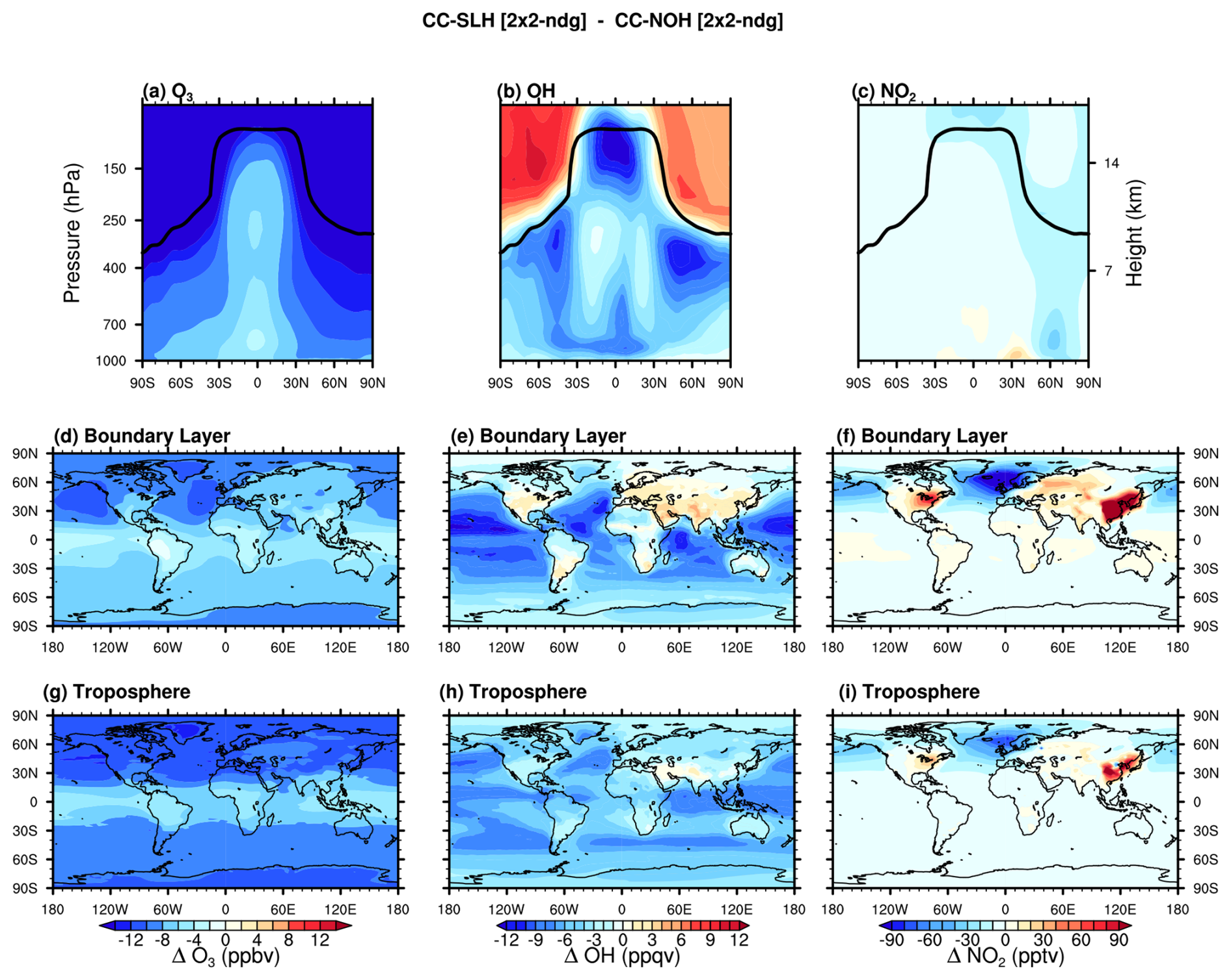
Figure 13 Geographical distribution of the SLH effect on the O₃, OH and NO₂ abundances during present-day (2015–2020) for the CC-SLH [2×2-ndg] experiment. First row: zonal average vertical distribution of (a) O₃, (b) OH and (c) NO₂. Second row: boundary layer mean (P≥850 hPa) for (d) O₃, (e) OH and (f) NO₂. Third row: tropospheric mean (surface up to the tropopause) for (g) O₃, (h) OH and (i) NO₂. The absolute differences computed as (CC-SLH [2×2-ndg] − CC-NOH [2×2-ndg]) are shown in all panels. Equivalent results with the percentage change are shown in Fig. 14.

Finally, the tropical VSL_I abundance is the lowest compared to the NH and SH extratropics due to the higher photochemical decomposition close to the Equator. In contrast, the I_y abundance in the tropics is larger than in the NH and SH extratropics due to the dominant tropical HOI/I₂ source (Fig. 1f). On the other side, surface VSL_Cl and VSL_Br tropical surface abundances lack of a pronounced seasonal cycle, although a regional seasonality is predicted in SGI_Br due to the changes in convective transport to the tropical tropopause layer (Fernandez et al., 2014, 2021). The double peak annual cycle in reservoir X_y observed within the tropics is attributed the seasonal changes in atmospheric rainout during the wet and dry seasons that affect the washout of inorganic halogens.

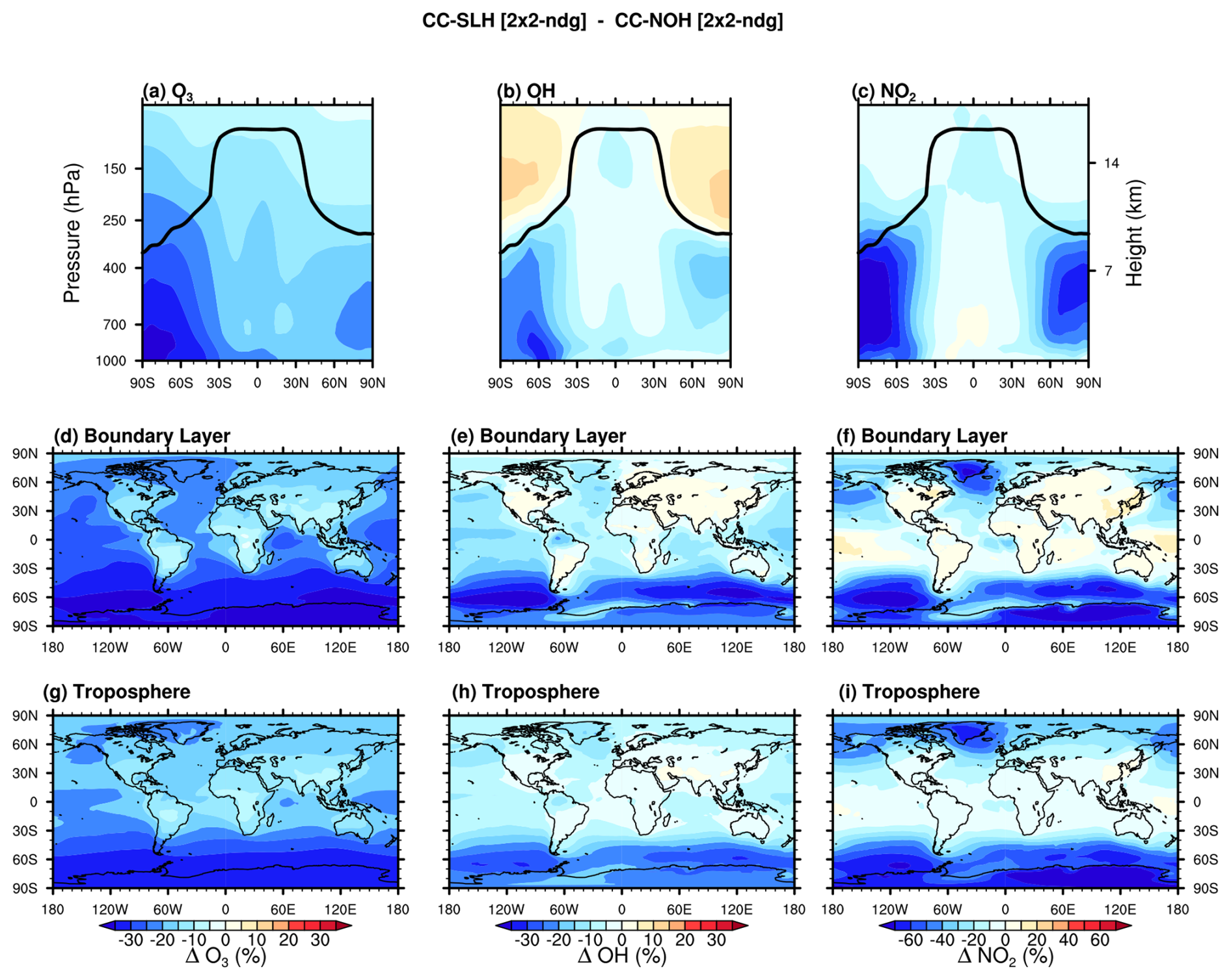
Figure 14 Geographical distribution of the SLH effect on the O₃, OH and NO₂ abundances during present-day (2015–2020) for the CC-SLH [2×2-ndg] experiment. First row: zonal average vertical distribution of (a) O₃, (b) OH and (c) NO₂. Second row: boundary layer mean (P≥850 hPa) for (d) O₃, (e) OH and (f) NO₂. Third row: tropospheric mean (surface up to the tropopause) for (g) O₃, (h) OH and (i) NO₂. The percentage differences computed as ((CC-SLH [2×2-ndg] − CC-NOH [2×2-ndg])/CC-NOH [2×2-ndg]) × 100 % are shown in all panels. Equivalent results with the absolute difference are shown in Fig. 13.

4.3 Influence of SLH on atmospheric composition

Table 9 presents the global mean O₃, OH and NO₂ abundance represented by the main CESM2-SLH compsets during the 2015–2020 period, distinguishing the absolute and percentage differences between equivalent simulations including (SLH) and neglecting (NOH) short-lived halogen chemistry. Including SLH chemistry in the model results in a substantial (16.9 %–17.3 %) reduction in the tropospheric ozone burden, decreasing from 336–345 Tg O₃ for the CC-NOH [2×2-ndg] and CC-NOH [2×2-hst] experiments to 278–287 Tg O₃ for CC-SLH [2×2-ndg] and CC-SLH [2×2-hst], respectively. Previous CESM1 estimations of stratospheric ozone depletion due to SLH were −5.2 DU (−2.0 %) (Saiz-Lopez et al., 2023), which falls within our CESM2-SLH simulated values of ozone depletion between −6.4 and −4.0 DU (−2.5 % and −1.6 %), respectively obtained with CC-SLH [2×2-ndg] and CC-SLH [2×2-hst] (see Sect. 4.3.4). Similar to ozone, SLH sources and chemistry globally reduce OH and NO₂. CESM2-SLH reductions range between −2.7% and −3.9% at the surface and approximately −6 % integrated in the troposphere for OH, while for NO₂ differences remain below −1 % at the surface and ranging between −7.2 % and −8.6 % in the troposphere.

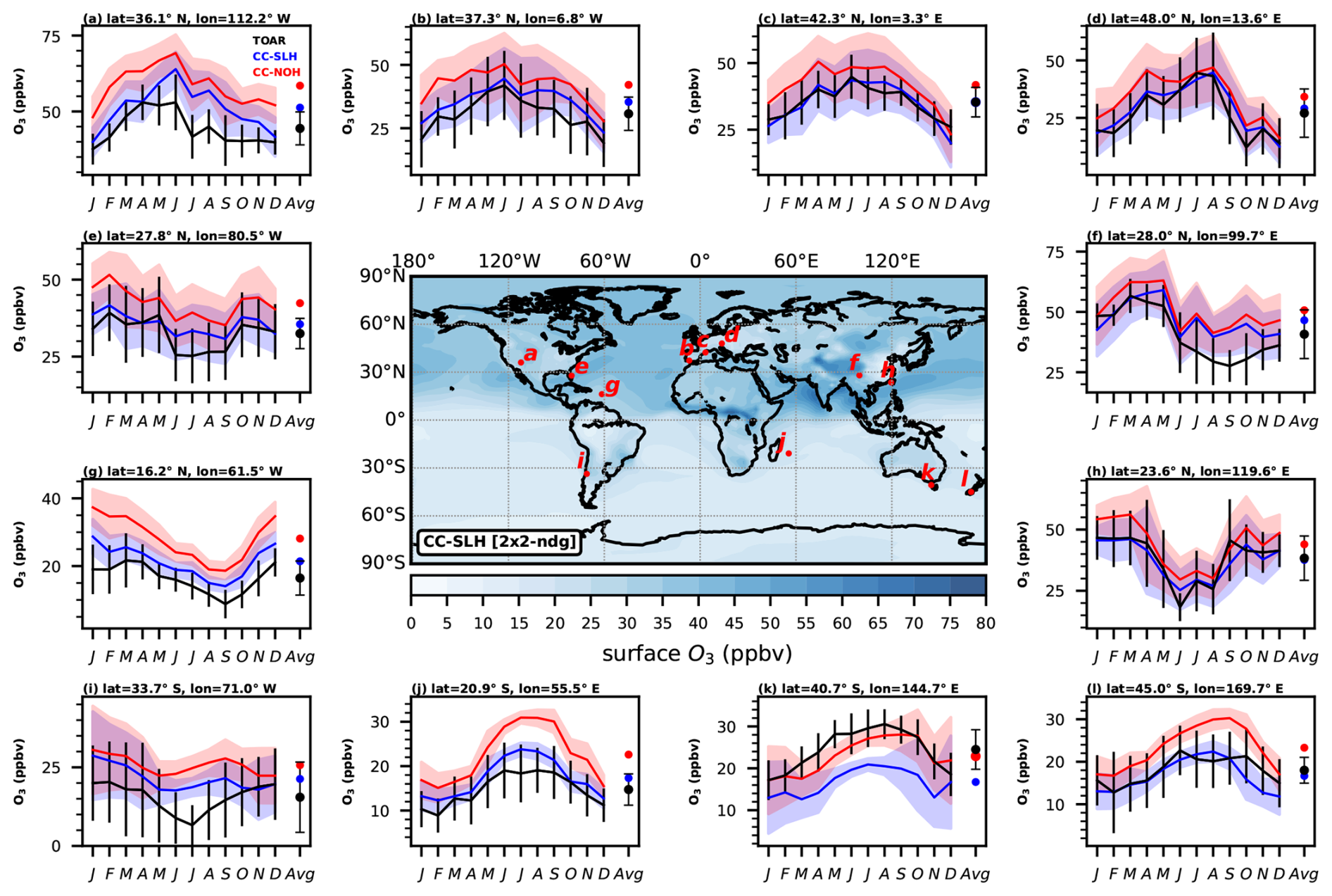
Figure 15 Comparison of CESM2-SLH nudged CC-SLH [2×2-ndg] and CC-NOH [2×2-ndg] simulations with TOAR-I observations. The center panel shows the geographical distribution of surface ozone for the CC-SLH [2×2-ndg] experiment, as well as the location of each of the observational sites shown in the side panels (red points). The side panels (a–l) show the monthly mean ± range seasonality (solid lines and shading) and the annual average (separate marker) of surface ozone for CC-SLH [2×2-ndg] (blue) and CC-NOH [2×2-ndg] (red) experiments. Black lines and error bars show surface observations reported in the first phase of Tropospheric Ozone Assessment Report (TOAR-I) (Schultz et al., 2017). Both model output and observations ranges have been computed as the standard deviation of hourly data for year 2015.

Figures 13 and 14 show the absolute and percentage change, respectively, induced by SLH over the atmospheric abundance of O₃, OH and NO₂ for the nudged experiments. SLH globally reduce the abundance of all species, particularly over the ocean and at high latitudes, with exception of some continental regions where the model shows an enhancement in OH and NO₂ abundance. The largest reductions in ozone mixing ratios occur in the lower stratosphere due to the high O₃ levels within the ozone layer, while percentage changes in the troposphere are larger than in the stratosphere. Similarly, the larger background ozone abundance over the NH results in larger absolute changes north of the Equator, while the largest percentage changes are observed in the SH, with minimum differences occurring over the tropical regions.

Given the dominant role of O₃ as the primary source of OH in the troposphere, the spatial distribution of OH changes follows that for O₃. However, and driven by its higher reactivity, OH changes are more pronounced than for O₃, with the largest reductions over the ocean as well as some continental enhancements (Bossolasco et al., 2025). In percentage terms, OH reduction due to SLH is lower over tropical regions, where most of the global tropospheric oxidation takes place. Maximum percentage differences are found over the pristine southern ocean due to the smaller contribution of the dominant secondary OH source driven by NO_x (see Sect. 4.3.2) compared with the north Atlantic and Pacific oceans, which presents the larger absolute differences. Similarly, the large NO₂ changes exceeding 50 pptv over continental regions barely represent a small percentage. The global mean change of surface NO₂ remains below ∼1 % (see Table 9).

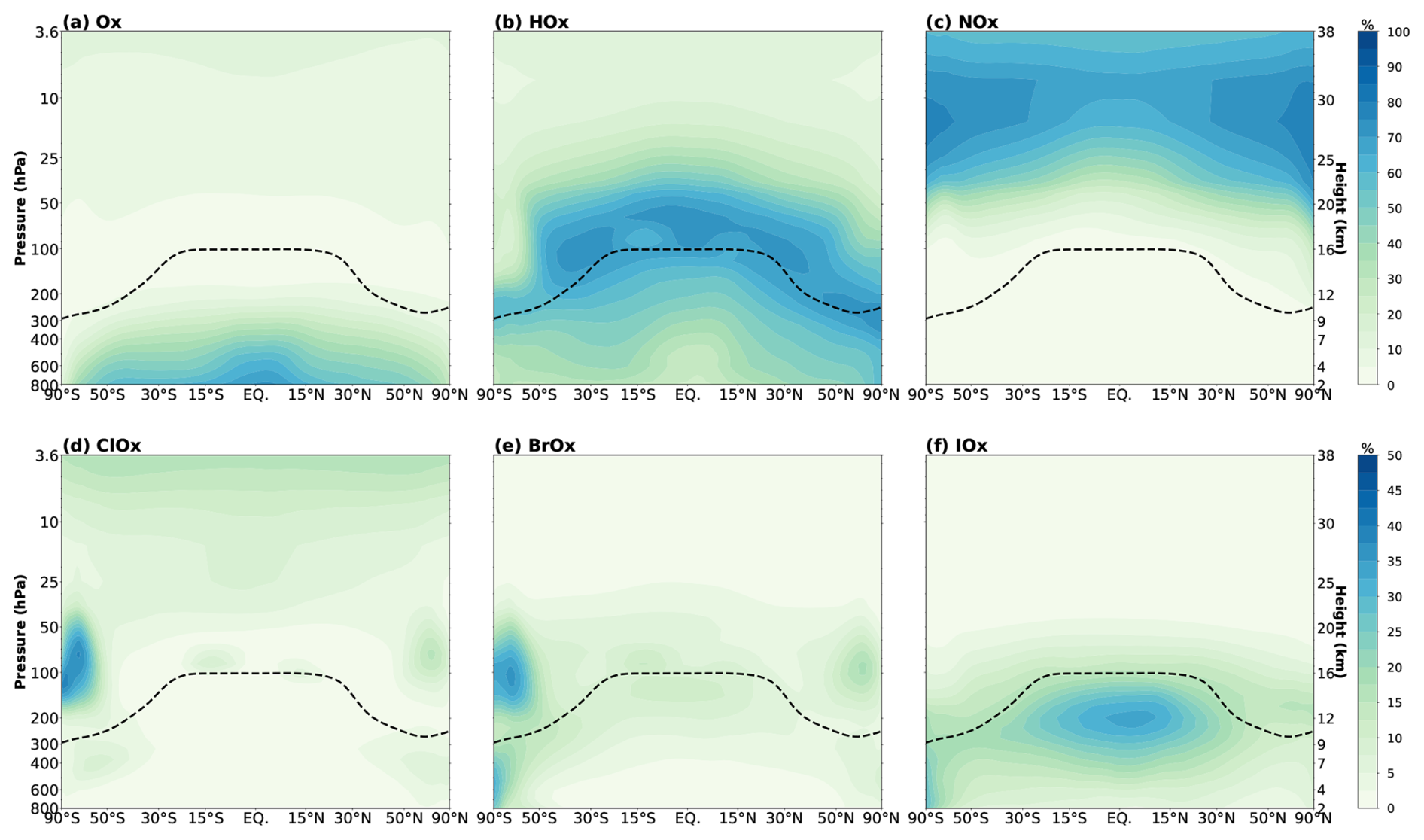
Figure 16 Zonal average distribution of Odd-oxygen loss rates (OddOx_Loss) for different ozone depleting families during present-day (2015–2020). Each panel presents the percentage contribution of each OddOx_Loss family to the total ozone loss for the CC-SLH [2×2-ndg] experiment. The top-row shows results for the main OddOx_Loss channels when SLH are not considered: (a) O_x, (b) HO_x and (c) NO_x loss cycles, while the bottom-row shows the percentage contribution from the individual halogen-driven OddOx_Loss cycles: (d) ClO_x, (e) BrO_x and (f) IO_x. The black-dashed line indicates the model mean tropopause.

4.3.1 Evaluation of model performance with air-pollutants

To evaluate the performance of CESM2-SLH, surface ozone abundance for the CC-SLH [2×2-ndg] and CC-NOH [2×2-ndg] experiments was compared with observations reported in the first phase of Tropospheric Ozone Assessment Report (TOAR-I; https://igacproject.org/activities/TOAR/TOAR-I, last access: 4 May 2026) (Schultz et al., 2017). The central panel in Fig. 15 shows the geographical distribution of annual mean surface ozone for CC-SLH [2×2-ndg] during year 2015, along with 12 surrounding panels showing the seasonal comparison with observational data at coastal or close-to-coastal locations (red points in central panel). The model reproduces the hemispheric asymmetry in surface ozone, with background levels below 40 ppbv in the pristine SH, contrasting with peak concentrations (60–75 ppbv) over continental and coastal Asia. Moreover, the ozone peak on the African continent is mainly linked to biomass burning. These maxima values are consistent with those reported by previous studies using CESM2 (Emmons et al., 2020). Moreover, Fig. 15 also shows a visual comparison of the monthly (lines) and annual mean (markers) surface ozone concentrations between the CC-SLH [2×2-ndg] (blue) and CC-NOH [2×2-ndg] (red) simulations and TOAR-I observations (black) across multiple stations located between extra-polar latitudes (60° N–60° S). Overall, the model captures the observed seasonal ozone cycles across most stations. This agreement is particularly strong at northern mid-latitude stations (>30° N), where the model reproduces both the magnitude and seasonality of ozone, with peaks in spring-summer driven by enhanced photochemical production. Similarly, good representation of ozone seasonality is observed at station (h) located in east Asia as well as in station (l) south of New Zeeland. Most notably, the inclusion of SLH chemistry results in an overall reduction of ozone that reduces the model bias and in most locations is larger than the spread of modelled values between the CC-SLH and CC-NOH experiments. However, discrepancies emerge at some stations like i) in central Chile, where the model successfully reproduces the observed ozone magnitude but fails to capture the seasonal cycle. This divergence likely stems from incomplete representation of ozone sources and sinks in this pristine region, as well as due to the coarse resolution used. Indeed, the coarse resolution of the model is well-known factor affecting the comparison with in-situ observations, as the local ozone values in some observational sites do not necessarily represent the mean background levels predicted over a 1.9°×2.5° pixel size. Nevertheless, Fig. 15 clearly shows that the inclusion of SLH chemistry in CESM2 helps to close the gap between the model and observations.

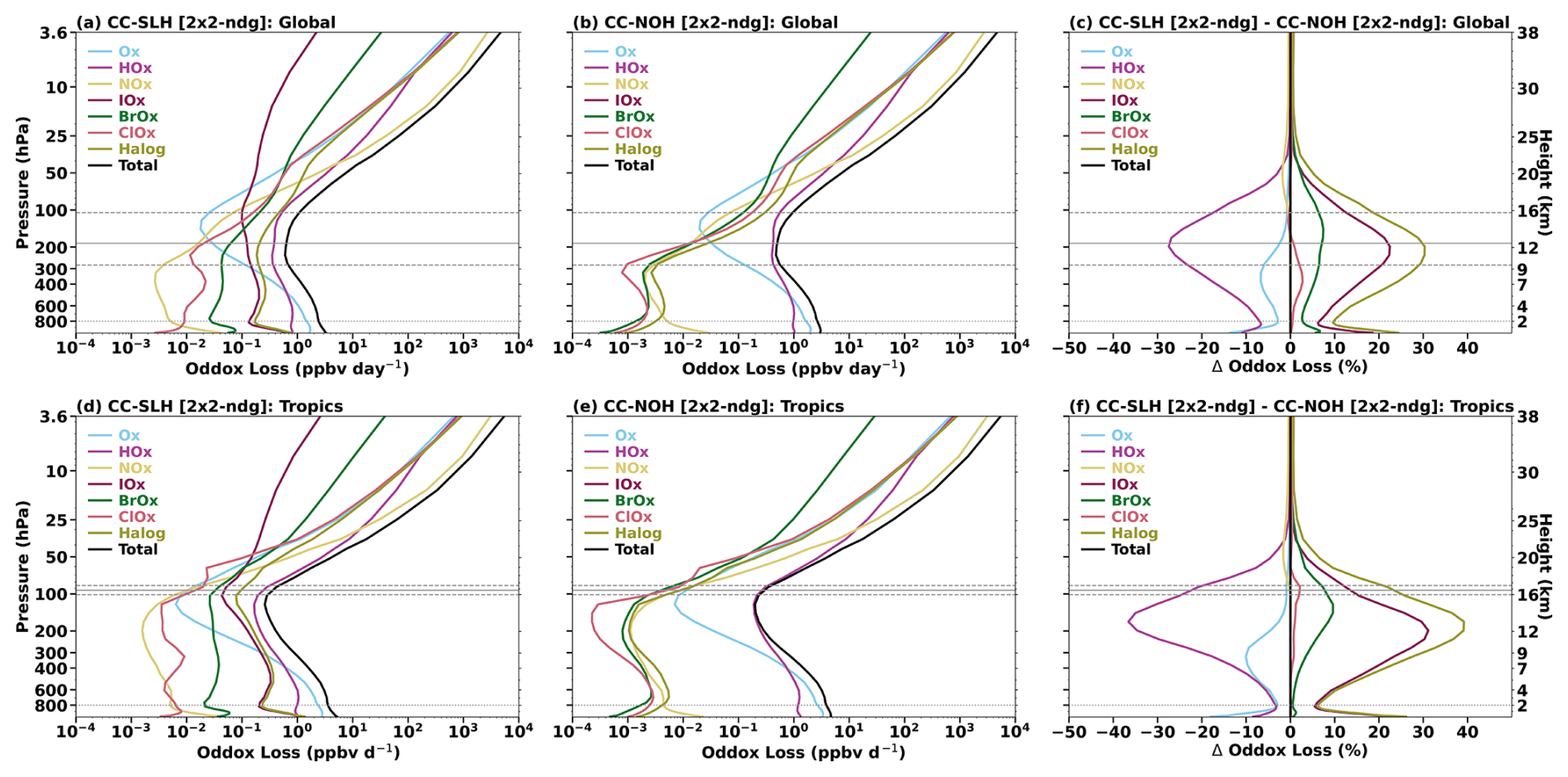
Figure 17 Vertical profile distribution of Odd-oxygen loss rates (OddOx_Loss) cycles during present-day (2015–2020) for nudged model experiments that (a, d) include and (b, e) neglect SLH sources and chemistry, respectively. Panels (c, f) show the percentage difference between both experiments computed as ((CC-SLH [2×2-ndg] − CC-NOH [2×2-ndg])/CC-NOH [2×2-ndg]) × 100 %. Results for the global mean (90° N–90° S) are shown in the top row while tropical mean (20° N–20° S) vertical profiles are shown in the bottom-row. The horizontal solid and dashed lines show the global or tropical mean tropopause height ± standard deviation, while the horizontal dotted line corresponds to P=850 hPa.

Table 10 Tropospheric ozone budget for nudged and free-running experiments including and neglecting SLH.

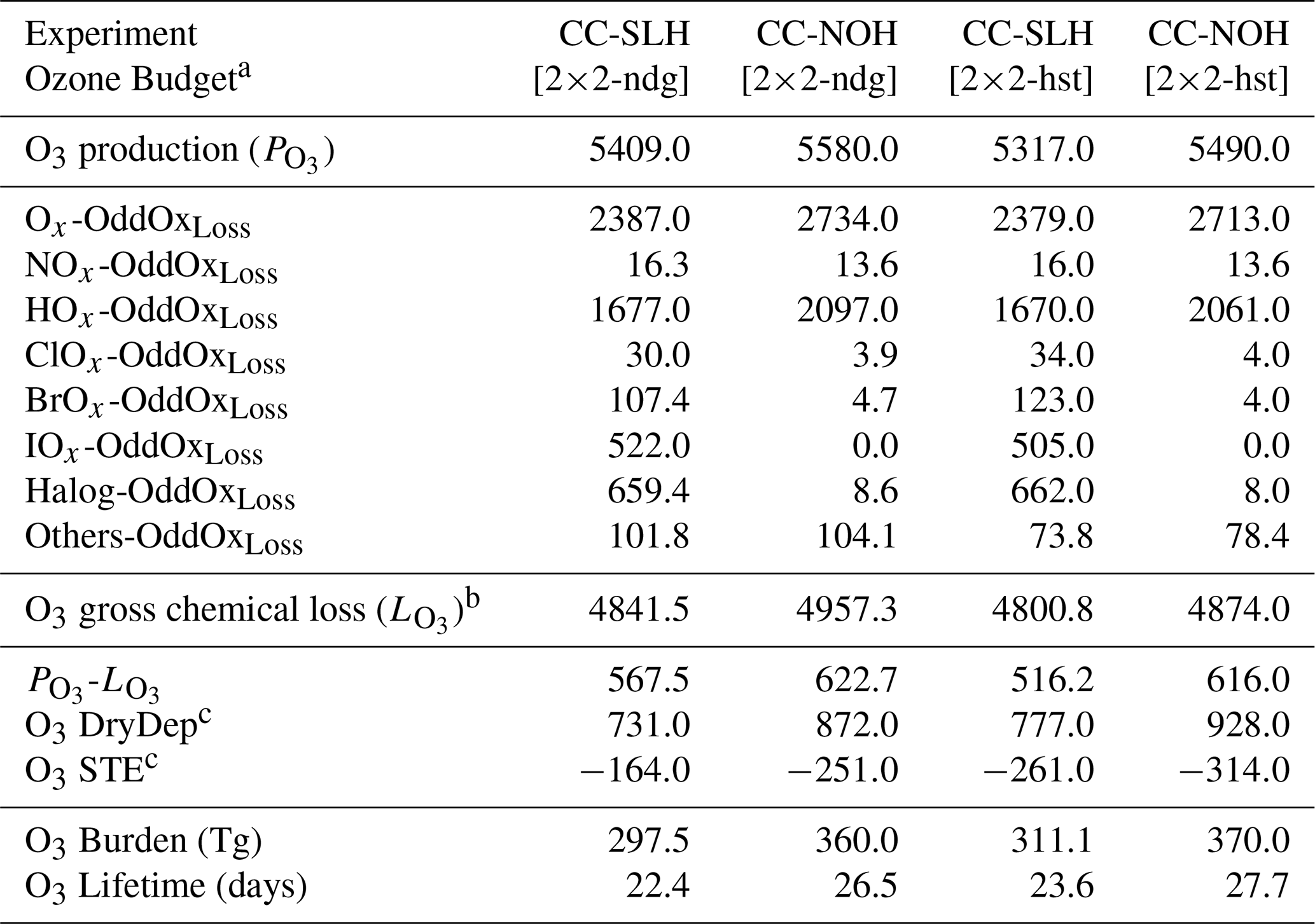
^a Unless stated otherwise, all tropospheric magnitudes are expressed in Tg yr⁻¹ and have been computed considering the internal model tropopause (TROP_P, hPa), defined as the pressure level where the minimum temperature lapse rate is derived. ^b The ozone gross chemical loss ($L_{{\mathrm{O}}_{\mathrm{3}}}$) is computed as the sum of all individual OddOx_Loss terms. ^c Stratosphere-to-Troposphere Exchange (STE) is computed as STE = $P_{{\mathrm{O}}_{\mathrm{3}}}$ − $L_{{\mathrm{O}}_{\mathrm{3}}}$ − DryDep, where $P_{{\mathrm{O}}_{\mathrm{3}}}$ is the O₃ photochemical production, $L_{{\mathrm{O}}_{\mathrm{3}}}$ is the gross chemical loss and DryDep is the ozone dry deposition.

4.3.2 Enhanced SLH-driven ozone chemical loss

This section highlights the effect of SLH on ozone destruction by means of computing the odd-oxygen chemical loss (OddOx_Loss) as performed in previous studies, following the definitions presented in Table 5 of Saiz-Lopez et al. (2014) (see Appendix for further details). Figure 16 shows the annual mean OddOx_Loss as a function of latitude and height for CC-SLH [2×2-ndg], where the individual contribution of the different families contributing to ozone depletion are distinguished. Going from top to bottom, in the upper stratosphere, OddOx_Loss is dominated by NO_x cycles (Fig. 16c), while from the middle and lower stratosphere down to the free-troposphere, the dominant OddOx_Loss family is HO_x (Fig. 16b) until O_x becomes the dominant ozone loss channel over the boundary layer (Fig. 16a). Note the halogen-driven OddOx_Loss shown in Fig. 16d–f maximize in the tropical upper troposphere (dominated by IO_x) and global lower stratosphere (both BrO_x and IO_x increase, with a minor role of ClO_x), where they contribute to additional ozone destruction. Most of this halogen-driven ozone loss results from: (i) faster recycling and gas-phase iodine chemistry compared to bromine and chlorine; and (ii) the larger conversion of iodine to reactive product gases occurring in the lower troposphere. In addition, note the important contribution of BrO_x and ClO_x cycles on ozone depletion over the Antarctic lower stratosphere of the southern hemisphere high latitudes (Fig. 16d and e), which maximizes during spring and is responsible for the formation of the Antarctic ozone hole (see Fig. 18).

Table 11 Global OH production for nudged and free-running experiments including and neglecting SLH.

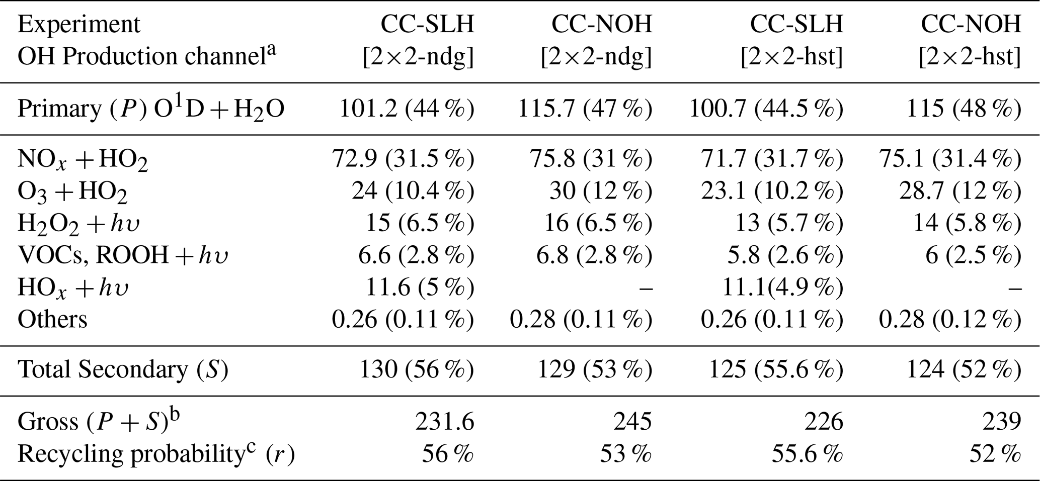
^a Unless stated otherwise, absolute OH production values for each channel are expressed in Tmol yr⁻¹. The corresponding percentage contribution of each channel with respect to the gross OH production is shown inside parenthesis. ^b The gross OH production expressed in Tmol yr⁻¹ is computed as $G=P+S$, where P is the primary OH production and S is the sum of all secondary channels (S). ^c The recycling probability (r) is expressed in percentage and is calculated as $\mathrm{1}-(P/G)\cdot \mathrm{100}$ %.

Figure 17 shows the mean vertical distribution of the dominant OddOx_Loss channels averaged globally (Fig. 17a–c) and within the tropical regions (Fig. 17d–f). To highlight the influence of SLH on tropospheric chemistry, we quantify in absolute terms the contribution from each family for the CC-SLH [2×2-ndg] and CC-NOH [2×2-ndg] experiments, as well as the differences between them in the right-most panel. The dominant ozone losses in the troposphere for CC-NOH [2×2-ndg] (Fig. 17a) are due to direct O_x photolysis, followed by HO_x cycles, both of which are significantly reduced when SLH are included, particularly in the lower and free troposphere (note NO_x only contribute significantly to OddOx_Loss in the middle and upper stratosphere). Indeed, for the CC-SLH [2×2-ndg] experiment (Fig. 17b), the total contribution of halogens increases significantly and represents between 10 % and 30 % globally (Fig. 17c), with a variable vertical profile that is dominated by IO_x cycles in the troposphere, and an increasing contribution mostly from BrO_x close to the tropopause. This increase in halogen driven ozone loss is compensated by a proportional decrease in the OddOx_Loss destruction by HO_x and O_x in comparison with CC-NOH [2×2-ndg] (negative change in Fig. 17c and f). Most notably, the largest halogen-driven contribution to total ozone loss is due to iodine chemistry, which represents up to 30 % within the tropical free troposphere in agreement with previous estimates (Saiz-Lopez et al., 2012, 2014), followed by bromine and with a minor contribution by chlorine.

4.3.3 Impact of SLH in the troposphere

Table 10 summarized the annual mean odd-oxygen loss channels, as well as the net chemical ozone production and net chemical change for the different simulations considered. Globally, the halogen driven tropospheric photochemical ozone destruction reaches 659.4 Tg yr⁻¹ for CC-SLH [2×2-ndg] and 662 Tg yr⁻¹ for CC-SLH [2×2-hst], dominated by IO_x-induced OddOx_Loss (accounting for 76 %–79 %) and with minor contributions for bromine (16 %–18 %) and chlorine (5 %). These values show excellent agreement with previously reported halogen influences obtained with CESM1 (Badia et al., 2021). Table 10 also shows that the tropospheric ozone photochemical production and the gross chemical loss remains almost unaltered (with minor changes below ∼3 %) regardless of the consideration or not of SLH sources and chemistry, consistent with previous studies (Barrera et al., 2023). In contrast, and driven mainly by the larger ozone destruction when SLH are considered, the estimated O₃ dry deposition is reduced by approximately 16 % for CC-SLH [2×2-ndg] and CC-SLH [2×2-hst] compared to their corresponding CC-NOH [2×2-ndg] and CC-NOH [2×2-hst] experiments, which is in line with the 11 % reduction previously estimated in CESM1. The net stratospheric to tropospheric exchange (STE) for CC-SLH [2×2-ndg] and CC-SLH [2×2-hst] reaches 164 and 261 Tg yr⁻¹, respectively. Even though in absolute terms the contribution of STE to the tropospheric ozone budget in CESM2-SLH is smaller than for CESM1 (e.g., STE accounts for 341 Tg yr⁻¹ for CESM1-SLH [SL23]), the inclusion of SLH compared to NOH results in an equivalent halogen-driven reduction in the contribution of STE of approximately 20 %, particularly for the nudging setup (Barrera et al., 2023). Differences between model versions are attributed to dynamical changes in the representation of air subsidence and downward ozone transport across the tropopause between the old and new nudging approaches (Davis et al., 2022) and will be evaluated in future studies.

Table 11 shows the most important chemical pathways contributing to the formation of OH, where the individual contributions have been separated between the dominant primary production (P), which is the production of O¹D by ozone photolysis at hν<330 nm followed by reaction with tropospheric water vapour; and secondary production (S), which accounts for all the remaining processes involving VOCs, NO_x and O_x (Lelieveld et al., 2016), as well as the reactions of hydrogen peroxide and halogenated hypohalous acids (Bossolasco et al., 2025). Due to the larger O₃ burden in CESM2-SLH compared with CESM1, we note that the changes in OH production are also expected to differ between the different model versions.

The tropospheric ozone depletion induced by SLH result in a reduction of P from approximately 116 Tg yr⁻¹ for the CC-NOH [2×2-hst] and CC-NOH [2×2-ndg] sensitivity simulations (which represent approximately 47 %–48 % of the total OH source) to approximately 101 Tg yr⁻¹ (44 %–45 %) for the main CC-SLH [2×2-hst] and CC-SLH [2×2-ndg] experiments. Similarly, the secondary ozone-driven pathway (O₃ + HO₂) reduces from approximately 12 % to 10 % due to the inclusion of SLH, inducing minor alterations in the other secondary channels that remain below a few percent (see Table 11). These reductions in P and S are compensated by ∼5 % increase in the contribution from the photolysis of HOCl, HOBr and HOI, which accounts for more than 11 Tg yr⁻¹ of the global annual production. Consequently, there is a continuous shift in the chemical OH production from primary to secondary sources, which implies that once formed, OH has an increased capability of being chemically re-generated in the atmosphere when SLH are considered. Therefore, SLH results in a net reduction of OH abundance while the tropospheric oxidation capacity of OH on a per atom basis increases. This is typically measured by computing the OH recycling probability, $r=\mathrm{1}-P/(P+S)$ (Lelieveld et al., 2016), which represents the capability of OH to be regenerated from secondary sources. Most notably, considering SLH in CESM2 increases r from approximately 52 %–53 % to 55 %–56 % (see Table 11).

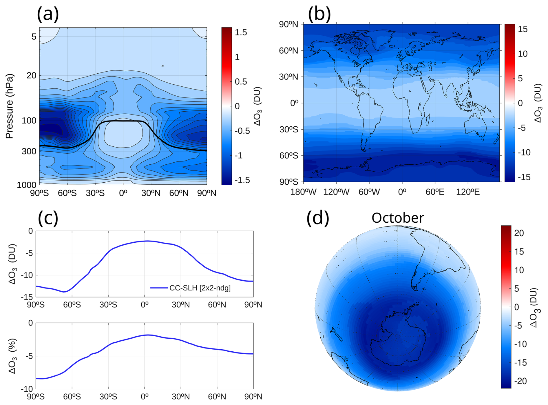
Figure 18 Column integrated ozone change (ΔO₃) in Dobson units (DU) between the CC-SLH [2×2-ndg] and CC-NOH [2×2-ndg] experiments during present-day (2015–2020). (a) Annual mean zonal average of ΔO₃. The solid black line shows the mean tropopause height. (b) Annual mean geographical distribution of ΔO₃ integrated across the lower stratosphere (from the tropopause to 20 hPa). (c) Annual mean absolute (top panel) and percentage (bottom panel) latitudinal distribution of integrated ΔO₃ in the lower stratosphere. (d) South-polar view of October ΔO₃ integrated in the lower stratosphere.

4.3.4 Impact of SLH in the stratosphere

This section presents the combined influence of SLH chlorine, bromine and iodine on stratospheric ozone in CESM2-SLH. Following previous studies (Saiz-Lopez et al., 2015; Fernandez et al., 2017; Cuevas et al., 2022; Barrera et al., 2023; Villamayor et al., 2023), we distinguish the effects observed over the global lower stratosphere from those affecting the Antarctic ozone hole. Figure 18a shows the annual mean change in O₃ associated with SLH, defined as the difference in O₃ partial column densities (DU) as a function of latitude and height between CC-SLH [2×2-ndg] and CC-NOH [2×2-ndg] (ΔO₃). This diagnostic highlights that the SLH influence on stratospheric ozone maximizes in the lowermost stratosphere, just above the tropopause (Fig. 18a), which is of major importance as the radiative perturbations in this region are highly sensitive to small changes in ozone abundance (Riese et al., 2012; Saiz-Lopez et al., 2012, 2023). Most notably, the SLH influence integrated in the lower stratosphere (from the tropopause to ∼20 hPa) presents a pronounced latitudinal variation, with ozone reductions increasing from the Equator and tropical regions to the mid-to-high latitudes (Fig. 18b and c). This is due to the larger conversion from SGI to PGI as air is transported from the tropical regions towards the poles through Brewer-Dobson circulation, combined with the lower temperatures prevailing at high latitudes that accelerate halogen chemical cycles. Here we note that SLH influence in lower stratospheric ozone is dominated by bromine and iodine chemistry (see Figs. 16 and 17), although the net effect is particularly sensitive to the background inorganic chlorine (Cl_y) levels in the stratosphere (Barrera et al., 2020; Villamayor et al., 2023). Therefore, the total SLH impact is expected to vary over time following the overall stratospheric chlorine loading before and after the peak in ODS observed in the stratosphere following the Montreal Protocol (WMO, 2018, 2022).

Figure 18b and c shows the net SLH-induced O₃ difference (ΔO₃) integrated over the lowermost stratosphere, where most of the SLH influence occurs. The resulting ΔO₃ for the nudged configuration ranges from −2.3 to 3.3 DU within the tropics (20° N–20° S) up to −9.5 to 13.8 DU for the high-latitudes (poleward of 60°). These ozone changes represent, respectively, −1.8 % to 2.7 % and −4.0 % to 8.4 % for the annual mean, depending on latitude. Current impacts are larger than those reported in previous CESM1 studies (Barrera et al., 2020; Fernandez et al., 2021), as those analyses only considered SLH bromine, while the CESM2-SLH simulations assessed here additionally include SLH iodine and anthropogenic VSL chlorine. Finally, Fig. 18d shows that stratospheric ozone destruction maximize during austral spring over the Antarctic polar vortex, where SLH bromine and iodine enhance the ozone hole deficit by more than −20 DU and −14 % during October, in agreement with previous reports based on CESM1 (Fernandez et al., 2017; Cuevas et al., 2022).

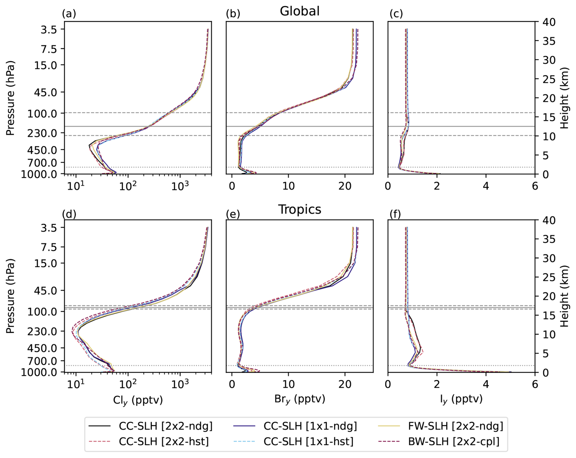
Figure 19 Comparison of global (90° N–90° S; a–c) and tropical (20° N–20° S; d–f) mean vertical profiles of total inorganic halogen abundance (X_y) between the 6 different CESM2-SLH experiments. Left, middle and right columns show results for (a, d) chlorine, (b, e) bromine and (c, f) iodine. The horizontal solid and dashed lines show the global or tropical mean tropopause height ± standard deviation, while the horizontal dotted line corresponds to P=850 hPa.

4.4 Comparison between different model experiments

All results using CESM2-SLH presented in previous sections have been performed using the FCnudged_slh and FCHIST_slh compsets with (2°×2°) resolution (i.e., CC-SLH [2×2-ndg] and CC-SLH [2×2-hst], see Table 7). Below we provide a first-order general intercomparison of organic VSLS and inorganic halogen distributions between different model configurations that is recommended to perform in order to validate model performance. A brief description of the main routines and user-defined namelist required to setup and modify different model experiments within CESM2-SLH is included in the Appendix.

Figure 19 shows a comparison of the tropical (20° N–20° S) and global (90° N–90° S) mean vertical profiles of Cl_y, Br_y and I_y for the six SLH experiments shown in Table 7, where the model output of high-top compsets using WACCM 70L have been interpolated with a bi-linear method (i.e., using NCAR interpic routine) to the default CAM6-Chem 32L vertical grid. All model experiments result in a very similar profile all the way from the surface to the upper stratosphere, although minor discrepancies in the vertical distribution remain. The corresponding tropospheric percentage changes range from −0.4 % to +20 % for bromine and −24 % to −0.2 % for iodine (see Fig. S7), where as expected, the largest percentage differences appear at those heights where the X_y abundance is small. For the particular case of surface Br_y, fine-resolution CC-SLH [1×1-hst] shows lower abundances than the coarse CC-SLH [2×2-hst] setup, while CC-SLH [1×1-ndg] and BW-SLH [2×2-cpl] experiments show larger values than CC-SLH [2×2-ndg] and FW-SLH [2×2-ndg], respectively. This is attributed to the smaller contribution from SSA-dehalogenation, particularly over the Southern Ocean. However, when integrated over the troposphere, note that the fine CC-SLH [1×1-hst] experiments present a larger Br_y burden than the coarse CC-SLH [2×2-hst] case, although smaller than those predicted for CC-SLH [1×1-ndg] and BW-SLH [2×2-cpl] (see Table S4). Chlorine, which of all halogen species shows the largest range in Cl_y abundance from the surface to the top of the model, results in tropospheric changes that remain below ∼7.5 % between the different compsets, with peak percentage differences predicted between BW-SLH [2×2-cpl] and FW-SLH [2×2-ndg] experiments close to the tropopause that are rapidly reduced below 10 % as soon as LLH_Cl are photodecomposed in the lower stratosphere.

Finally, Fig. S8 shows a comparison of the VSLS zonal average for the different SLH experiments, where all distributions have been averaged for the 2000–2005 period. Most notably, all experiments show equivalent distributions for all halocarbons and inorganic halogens, with slightly lower values in the NH high-latitude free troposphere for the finer resolution (1°×1°) grids, particularly for VSL_Cl (see Fig. S8g and j). Similarly, Fig. S9 shows the geographical distribution of Cl_y, Br_y and I_y abundance averaged within the boundary layer for the different model experiments. Although all compsets show comparable global distributions and mean values, we highlight that the maximum abundance and partitioning between reactive and reservoir species within regional hot-spots present significant differences. Particularly remarkable are the Br_y differences between CC-SLH [2×2-hst] and BW-SLH [2×2-cpl] over the North Atlantic and North Pacific oceans, as well as over the Southern Ocean. This is coherent with the larger SSA-dehalogenation sources simulated in these regions, which affect the BrO/Br_y partitioning. Similarly, the higher resolution experiments CC-SLH [1×1-ndg] and CC-SLH [1×1-hst] display greater Cl_y abundances over the oceanic outflow of polluted air masses from Europe, Eastern US and East Asia (see Fig. S9g and j). This is associated with the enhancement of the acid-displacement reaction occurring when HNO₃ air-masses are mixed with SSA-rich oceanic fresh air. Table S4 summarizes the comparison of the global mean surface and tropospheric halogen abundance of halogenated VSLS and inorganic halogens across the different model experiments, while Table S5 compares the change in O₃, OH and NO₂ abundance between CC/FW/BW-SLH and CC/FW/BW-NOH simulations.

5 Discussion

In this section we highlight the scientific relevance and limitations of including comprehensive halogen chemistry in CESM2-SLH in comparison with previous studies and other models, pointing out the main drivers controlling halogen abundance and distribution in the global atmosphere (Sect. 5.1) as well as the implications for quantifying changes in tropospheric oxidative capacity and stratospheric ozone depletion (Sect. 5.2). In Sect. 5.3 we introduce a comprehensive set of recommendations that should be considered not only for interpreting current results, but mostly for new users willing to perform their own scientific studies using CESM2-SLH.

5.1 Representation of halogen abundance in the global atmosphere

Although organic VSLS are not the primary source of reactive halogens in the boundary layer, their photodecomposition constitutes a critical first step in releasing inorganic chlorine, bromine and iodine to the atmosphere, followed by subsequent gas-phase and heterogeneous-phase reactions that partition inorganic halogens between reactive and reservoir species. These initial release of halogens can be amplified through non-stoichiometric heterogeneous recycling processes, particularly via SSA-dehalogenation, which constitutes the dominant halogen source for chlorine and bromine in the lower troposphere (see Fig. 10). In particular, VSL_Cl photodegradation represents only a minor contribution to atomic Cl release in the troposphere, which is largely dominated by the online acid-displacement emissions. The quantitative analysis presented in Sect. 4.1 and 4.4 shows that the overall tropospheric and stratospheric halogen abundance obtained with the current CESM2-SLH release is equivalent to (and in any case, smaller than) that implemented in previous CESM1 and other global models such as EMAC, TOMCAT and GEOS-Chem (Saiz-Lopez et al., 2012, 2023; Sinnhuber and Meul, 2015; Hossaini et al., 2016; Sherwen et al., 2016b). This highlights that the influence of chlorine, bromine and iodine in tropospheric oxidative capacity and stratospheric ozone depletion in CESM2-SLH represents a lower limit compared to previous studies.

The current CESM2-SLH configuration applied ∼15 % enhancement to oceanic VSL bromo- and chloro-carbons to reproduce previous CESM1 distributions. This resulted in SG vertical profiles and trends that lay in the lower margin of the most recent assessment of VSL_Cl contribution to chlorine stratospheric injection (Fig. 5a). Therefore the offline emissions and LBCs for anthropogenic chlorinated halocarbons described in Sect. 2.1.2 could have been increased by a factor larger than the 15 % enhancement considered here to reproduce the observed trend in the recent past (WMO, 2022). However, we acknowledge that several other factors influence the regional enhancements and recent trends of chlorinated VSLS in the lower stratosphere (Hossaini et al., 2024). Due to the large anthropogenic contribution from developed regions over US, Europe and Asia (Hossaini et al., 2019; Claxton et al., 2020), the VSL_Cl distribution for the Northern and Southern mid-latitudes shown in Fig. 7 shows a clear hemispheric asymmetry just below the tropopause. This asymmetry on VSLS distributions have already been described in the literature for chlorine (Roozitalab et al., 2024) as well as bromine (Keber et al., 2020; Jesswein et al., 2022), although note that anthropogenic VSL_Br sources are currently not considered in CESM2-SLH.

Given that chlorine influence on stratospheric ozone is dominated by long-lived CFCs and HCFCs, the current model underestimation of SGI_Cl does not introduce a significant bias in the total stratospheric chlorine budget and, consequently, does not substantially affect chlorine-driven ozone destruction. Indeed, equivalent Cl_y changes in the upper stratosphere are predicted for all CC-SLH and CC-NOH experiments (see Fig. 19). Similarly, most of the organic LLH_Br conversion to reactive Br_y occurs in the lower stratosphere while most of VSL_I is rapidly photo-decomposed before reaching the tropopause (Figs. 7 and 8). Therefore, an adequate representation of the SGI and PGI of bromine and iodine occurring over the tropical regions (Fig. 4) is of major importance to properly quantify the SLH influence on lowermost stratospheric ozone. All free-running and nudged experiments show an equivalent stratospheric bromine and iodine loading regardless of the compset considered, with exception of BW-SLH [2×2-cpl] that results in a larger abundance of Br_y at the model top by ∼1 pptv compared to the other experiments. Most notably, our sensitivity analysis shows that after long-lived and short-lived halogens have been converted to inorganic chlorine, bromine and iodine, the modelled ΔCl_y, ΔBr_y and ΔI_y, between the different experiments remain below ∼5 %.

5.2 Influence of SLH on atmospheric composition

Given the general higher ozone abundance in base CESM2 CAM6-Chem compared to CESM1 CAM4-Chem (Emmons et al., 2020, see Fig. 2), the absolute SLH-driven tropospheric and surface ozone reductions are larger for current CESM2-SLH simulations compared to previous studies. However, we highlight that the corresponding percentage decreases of global mean ozone at the surface (∼22 %) and the troposphere (∼17 %) obtained in CESM2-SLH are in very good agreement with previous CESM1 studies, ranging from −13 % to −24 % at the surface and −16 % to −2 0% in the troposphere (Iglesias-Suarez et al., 2020; Badia et al., 2021; Barrera et al., 2023; Saiz-Lopez et al., 2023). Nevertheless, we note that some discrepancies remain due to several SLH developments not yet implemented in CESM2-SLH (such as continental inorganic halogens, emissions from dust and/or polar halogens, see Sect. 3.3), as well as due to the continuous improvements implemented in the base CESM development branch, which directly or indirectly impact on SLH abundance and chemistry.

The tropospheric OH burden of 222.8–226.2 Mg obtained for nudged CC-SLH [2×2-ndg] and free-running CC-SLH [2×2-hst] experiments corresponds to a global mean tropospheric OH concentration of approximately 1.23–1.27×10⁶ molec. cm⁻³, consistent with previous model results neglecting SLH chemistry (Lelieveld et al., 2016) and in the higher edge of the range reported in the literature for the 21st century ($\mathrm{11.7}\pm \mathrm{1.0}\times {\mathrm{10}}^{\mathrm{5}}$ molec. cm⁻³; Voulgarakis et al., 2013). While the relative contribution of SLH to OH production and loss remains consistent between CESM1 and CESM2-SLH (Table 11), the absolute OH burden is substantially higher in CESM2-SLH compared to CESM1 (Table 9). This discrepancy is not attributable to the implementation of SLH sources and chemistry, but rather due to structural changes in between CESM versions, including updates in VOCs degradation, pollutant emissions, prescribed LBCs and the overall atmospheric oxidative capacity of CAM6-Chem relative to CAM4-Chem (Emmons et al., 2020). Although the absolute values of P and S differ between CESM1 and CESM2-SLH due to the different background state of the modelled atmosphere, the overall magnitude and relative contribution of the dominant OH production pathways remain consistent with previous studies using CESM1 and other global chemistry models (Bossolasco et al., 2025).

Other global models including SLH sources and chemistry, many of them following the original implementation in CESM (see Sect. 2), result in equivalent atmospheric composition changes as those summarized in Tables 9–11 for CC-SLH [2×2-ndg] and CC-SLH [2×2-hst] and Table S5 for the remaining experiments. For example, Sherwen et al. (2016b) estimated a global mean OH concentration of 1.27×10⁶ molec. cm⁻³ in GEOS-Chem that is ∼8 % lower than in a simulation without SLH, while the addition of tropospheric halogens in LMDZ-INCAA leads to ∼22 % decrease in tropospheric ozone and approximately −8 % in OH (Caram et al., 2023), although their predicted reduction in NO_x (∼33 %) is almost 4 times larger than in CESM2-SLH. Compared to CESM1, the percentage change in CESM2-SLH is smaller for OH and larger for NO₂ (see Table 9). Note that not only the absolute abundance but also the HO₂ $/$ OH and NO₂ $/$ NO ratio are significantly different between CESM1 and CESM2 (see Fig. 2k and l), all of which impact on the estimated global mean values. Given the large number of factors influencing the rapid interconversion between HO_x and NO_x species, such as the strength and spatial distribution of sources and the changes in chemical schemes between CESM versions, a deeper analysis of the dominant processes controlling these changes should be subject to future studies.

5.3 User recommendations for CESM2-SLH

Given the large spatio-temporal variability of Cl_y, Br_y and I_y within different regions of the atmosphere, we recommend new-users not familiarized with SLH chemistry to initially select the coarse (2°×2°) resolution, particularly with the FCnudged_slh compset. This ensures that atmospheric transport and temperature are consistently represented across simulations, which is crucial for isolating and quantifying chemical perturbations from dynamical variability between different model simulations. Despite a high-spatial resolution being available (see Table 7), we recommend new users to select the coarse resolution setup as many of the online photochemical sources and recycling reactions described in Sect. 2 depend on highly variable resolution-dependent atmospheric fields, such as SAD_SSA and SAD_ice, which typically show larger variability with increasing resolution (see Tables S4 and S5). Similarly, we found that resolution-dependent scaling factors for lightning-NOx production typically used in CESM2 (Emmons et al., 2020; Wild et al., 2020) result in significant alterations of the chemical partitioning and washout efficiency of SLH. Therefore, caution should be taken when moving from a coarse to a fine resolution, as the resulting halogen abundances can significantly vary between them. We highlight that all values and results presented in Sect. 4.4 were obtained considering the compset- and resolution-specific &slh_nl scaling factors compiled in Table A1, which should be taken as the starting point to adjust SLH and X_y abundance in CESM2-SLH. In case other model configuration is preferred, we strongly recommend performing an equivalent model intercomparison as the one provided in Sect. 4.4 to ensure that the global halogen sources and budgets are within the ranges of the many model experiments compiled in this work.

For the particular case of the FCnudged_slh and FWnudged_slh compsets, the scaling factors compiled in the Appendix for VSLS emissions, SSA-dehalogenation and washout following FRA were adjusted considering the default meteorological MERRA2 dataset (Rienecker et al., 2011). However, we note that all &slh_nl values are affected by changes in the dynamical transport, and must be fine-tuned in case other meteorological fields are imposed, as for example those from the fifth generation ECMWF (European Centre for Medium-Range Weather Forecasts) reanalysis (ERA5, 2023). See the Appendix and the CESM2-SLH Mendeley repository for further details (Fernandez et al., 2026b).

6 Summary and conclusions

In this work, we provide a comprehensive summary of the major scientific advances in our understanding of SLH emissions and chemistry on the global atmosphere as well as a complete description of the technical implementation of the main related processes and parameterizations in the widely used CESM chemistry-climate model. The new CESM2-SLH version includes a detailed representation of the main organic halocarbon and natural inorganic sources, as well as the gas-phase and heterogeneous chemistry of chlorine, bromine and iodine in the marine boundary layer, free troposphere and lowermost stratosphere, highlighting the dominant processes determining the role played by SLH on atmospheric composition. We have evaluated SLH global budgets, chemical partitioning and spatio-temporal distributions, with a special focus on the regional and global implications of SLH on tropospheric oxidizing capacity and stratospheric ozone. Although during the past 15 years most of the SLH developments had already been reported in several studies using different versions of CESM1, the current work provides a unified and comprehensive description integrated in the context of the latest model developments made within the Community Earth System Model framework. This development is a porting of our previous SLH experience and codes in CESM1, and therefore we aimed for new model results to be as similar as possible to those obtained in previous studies, all of which had been validated against multi-platform observations to date. In the future, as more observations become available, new validation efforts will allow further improvements to CESM2-SLH, particularly in the representation of heterogeneous recycling processes. We expect that new developments in the base version of CESM2, such as the improvements in the representation of sea-salt aerosol fields and atmospheric dynamics, would also help to reduce the remaining model biases, particularly for local domains with high-resolution. Indeed, the main drivers of the different modelled trends in O₃, OH, NO₂ and VOCs between CESM1 and CESM2 are the changes in the benchmark air-pollutant emissions, as well as on the updates on the chemical degradation and speciation of large hydrocarbons.

The current CESM2-SLH release comprises six new model compsets and includes a complete set of configuration files and parameters that must be properly set up with user-defined namelist options. These include increasing the number of default emission sources and prescribed LBCs, as well as expanding the list of species that suffer dry- and wet-deposition, including those that are taken up on ice. Similarly, a new set of initialization and absorption cross-section files, including updated data for VSLS and inorganic halogen species, are now available. Most notably, and with the intention of avoiding unintended misevaluation of SLH influence on atmospheric composition for users familiarized with current CESM2 compsets typically used for climate and air quality studies on the global scale, this work provides a general but complete intercomparison of organic VSLS and inorganic halogen distributions between previously published CESM1 results and a comrehensive set of CESM2-SLH experiments and resolutions. Given the important role played by SLH in tropospheric and stratospheric chemistry, as well as their changing influence depending on many Earth's system components that, in turn are linked to background atmospheric composition and climate, we call the wider CESM community to employ the CESM2-SLH release to obtain a realistic representation of the background influence of natural and anthropogenic short-lived halogen sources and chemistry in air quality and Earth's climate studies. Similarly, we encourage other global chemistry-climate models and regional chemistry-transport models to implement equivalent representations of SLH sources and chemistry to improve their representation of the natural halogen baseline in the atmosphere.

Appendix A: CESM2-SLH user's guide

Given that original SLH developments were performed on top of a discontinued CESM1 version that is no longer maintained by the community, the current CESM2-SLH implementation is presented and sustained with a double purpose: to be easily configured by CESM2 users that are not initially familiarized with SLH chemistry; and to allow the wider scientific community to evaluate the global mean influence of SLH in atmospheric chemistry and their implications for the Earth's climate system.

The updates in the CESM2-SLH release include:

• i.

  increasing the total number of halogenated species considered in the chemical mechanism, for some of which various species independent deposition velocity and Henry coefficients are required;

• ii.

  extending the number of species for which offline and online emissions are considered, as well as those that are included as LBCs;

• iii.

  replacing the absorption cross-section files to include new SLH species that are not available in the default CESM2 files;

• iv.

  incorporating a new namelist group section for SLH (&slh_nl) along with additional namelist variables to consider independent ice-uptake efficiencies for some halogen species;

• v.

  expanding the total number of default namelist files that provide individual namelist values for the different SLH configurations and user's cases;

• vi.

  including pre-compiled chemical mechanism with all SLH updates for CAM-Chem and WACCM; and

• vii.

  mapping and updating the original compsets available in the benchmark CESM2.2.0 version to directly create and compile the different CESM2-SLH model cases.

Chart S1 in the Supplement shows the main Fortran files that have been updated within the CESM2-SLH CAM6-Chem release (blue), highlighting in green the new ones specifically created for SLH chemistry. These modules and routines constitute the freeze state of the CESM2-SLH release and should be used as the starting point of any further developments related to SLH sources and chemistry. Additional building-scripts and configuration files are required to build and compile the new SLH compsets (Chart S2). As suggested by CESM developers, only expert users should introduce updates to these configuration files. Finally, Chart S3 highlight the main changes that must be applied to the default CESM namelist variables to properly configure any CESM2-SLH simulation based on the FCnudged_slh and FCHIST_slh compsets (equivalent changes shall also be applied to FWnudged_slh and BWHIST_slh compsets). These mandatory SLH namelist updates include:

• Initialization file: the initial condition (ncdata) data has been expanded from the default CESM initialization files with stabilized ODSs and GHGs and replaced to ensure background SLH species and related atmospheric compounds such as O₃ and OH are in steady state. Note that while 3 years of spin-up are sufficient to achieve tropospheric stabilization of SLH SGs and PGs, for studies focused in the stratosphere we recommend performing at least 7–10 years of spin-up when starting from an initial condition that neglects SLH.

• Offline emissions: the srf_emis_specifier within the &chem_inparm group has been expanded to include the offline emissions of CHBr₃, CH₂Br₂, CH₂BrCl, CHBr₂Cl, CHBrCl₂, CH₃I, CH₂I₂, CH₂IBr, CH₂ICl, CH₂Cl₂, C₂Cl₄, I₂, and HOI. Note that although HOI and I₂ are included in this list, this serves just as a placeholder as their emissions are forced to zero after being read and are subsequently computed online within the iodine_emissions.F90 routine.

• Boundary conditions: CH₃Cl and C₂H₄Cl₂ have been included in the flbc_list within the &chem_surfvals_nl group, as these species contribute to the atmospheric SLH chlorine loading. Updated flbc_file options including the projected trend of anthropogenic VSLS for the different SSPs have also been developed.

• Absorption cross-sections: to compute the photolysis of gas-phase organic and inorganic halogen species, wavelength-dependent absorption data of several SLH have been added to the default short-wave (xs_short_file) and temperature-dependent long-wave (xs_long_file) cross-section files within &chem_inparm.

• Dry deposition: the following species have been included in the drydep_list within &drydep_inparm: ClONO${}_{\underset{\mathrm{¯}}{\mathrm{2}}}$, HCl, HOCl, ClNO₂, BrONO${}_{\underset{\mathrm{¯}}{\mathrm{2}}}$, HBr, HOBr, BrNO₂, Br₂, IONO₂, HI, HOI, INO₂, I₂O₂, I₂O₃, I₂O₄, CHCl₂O₂, and COCl₂. The underlined species were already included in the default CESM2 setup.

• Wet deposition: the gas_wetdep_list within section &wetdep_inparm has also been extended with the following species: ClONO${}_{\underset{\mathrm{¯}}{\mathrm{2}}}$, HCl, HOCl, COFCl, BrONO${}_{\underset{\mathrm{¯}}{\mathrm{2}}}$, HBr, HOBr, ClNO₂, BrNO₂, Br₂, BrCl, IONO₂, INO₂, HI, IO, OIO, ICl, IBr, I₂O₂, I₂O₃, I₂O₄, CHCl₂O₂, and COCl₂. Additionally, the new namelist variable gas_wetdep_ice_uptake_list was included with the following halogen variables: HNO${}_{\underset{\mathrm{¯}}{\mathrm{3}}}$, ClONO₂, HCl, HOCl, BrNO₂, ClNO₂, I₂O₂, I₂O₃ and I₂O₄,. Note that ice_uptake=.true. is always imposed for HNO₃ within mo_neu_wetdep.F90 by default.

• SLH scaling factors: the new &slh_nl namelist section was incorporated, providing a set of scaling factors intended to adjust the recycling efficiency of the main processes affecting SLH sources and sinks when shifting between configurations.

All changes related to the implementation of offline oceanic VSLS sources have been performed in routines mo_srf_emissions.F90 and mo_usrrxt.F90 within the chemistry/mozart folder. To include the offline VSLS emissions from the Ordóñez et al. (2012) inventory, users just need to include the name of the species within the srf_emiss_specifier namelist option, and point at the specific file for each individual species. For the case of offline anthropogenic VSL chlorocarbons, in addition to increasing the srf_emiss_specifier namelist option with CH₂Cl₂ and C₂Cl₄, users should expand the flbc_list to include CHCl₃ and C₂H₄Cl₂. Differing from natural VSLS sources, anthropogenic VSLS emissions included in mo_srf_emissions.F90 present a flat hourly profile (i.e., no diurnal variation as shown in Fig. S1 is applied).

Table A1 Adjusted values of &slh_nl scaling factors for each of the main CESM2-SLH compsets and resolutions.

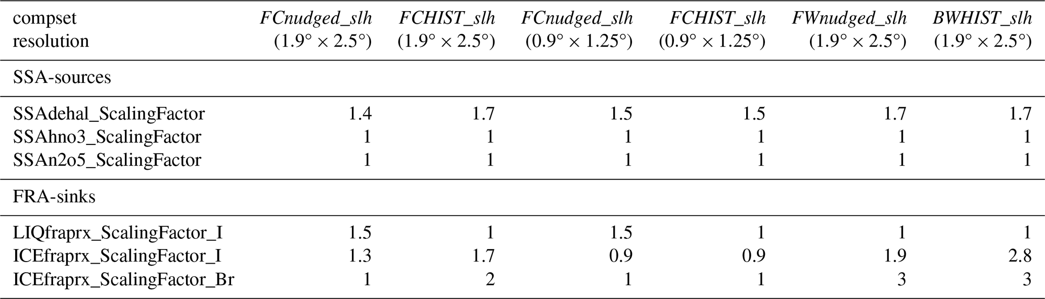
Online oceanic sources for inorganic iodine are included by adding variables HOI and I₂ to the standard srf_emiss_specifier used for offline VSLS, although the imposed offline iodine file represents just a place-holder as the input values are forced to zero after being read within mo_srf_emissions.F90 routine and replaced by the online computation performed in iodine_emissions.F90. For the case of SSA-dehalogenation reactions (see Table 1 in the main text), individual reactions are included in the chem_mech.in scheme and must be recompiled by the chemical pre-processor in case any change is applied (i.e., turn them off). Similarly, any alteration of stoichiometric reactions altering the SLH partitioning (Tables 2 and 3) as well as the washout of iodine and bromine species occurring through the Free-Regime Approximation (FRA, Tables 4 and 5), requires of recompiling the pre-compiled chemical mechanism. To allow a direct adjustment of the SSA-dehalogenation source-strength for different representations of sea-salt aerosol loadings, the current release incorporates a new SLH namelist section (&slh_nl; see Chart S3) with individual scaling factors for chlorine, bromine and iodine reservoirs, as well as for N₂O₅ and HNO₃ recycling (see Table A1). All of these stoichiometric and non-stoichiometric reactions and scaling factors for inorganic halogen reservoirs have been implemented in mo_usrrxt.F90. Finally, dry and wet deposition for halogen species has been implemented in modules mo_drydep.F90 and mo_neu_wetdep.F90, respectively. In the latter case, we introduced the additional variable gas_wetdep_ice_uptake_list within the &wetdep_inparm namelist group to avoid mapping the ice-uptake of halogen species to that of HNO₃ as originally implemented in CESM2.

Overall, the final SLH chemical mechanism implemented in CAM6-Chem introduces 12, 9 and 19 additional chlorine, bromine and iodine species that participate in 67, 53 and 93 new reactions, respectively. These new reactions are categorized as: photolysis, odd-halogen reactions, organic-halogen reactions, sulfur-halogen reactions, heterogeneous recycling on tropospheric aerosols, sea-salt recycling, and stratospheric mapped reactions (see Table A2), where some of the reactions involve inter-halogen interactions (e.g., ClO + BrO), and therefore are double-counted within each family. The inclusion of SLH chemistry in CESM2 results in an increment of the computational cost of ∼20 %–25 %.

Table A2 Total number of additional gas-phase and heterogeneous-phase halogen reactions included in CESM2-SLH chem_mech.in.

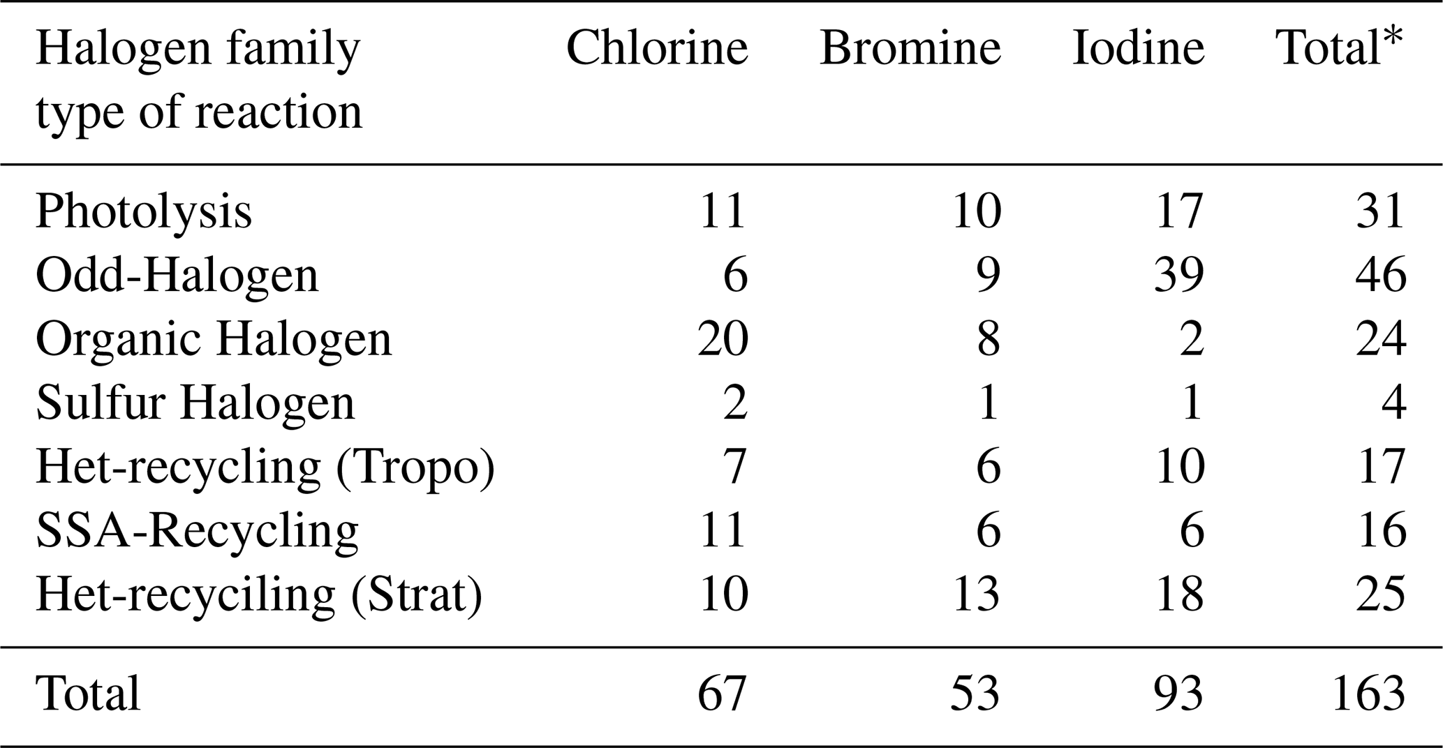
^* Some reactions involve inter-halogen interactions (e.g., ClO + BrO) and are double-counted within each halogen family. Therefore, the total reaction sum by halogen families is not additive. The complete list of halogen reactions is provided in main Tables 1–5 and S1–S3.

Finally, we note that current CESM2-SLH release includes only the SLH compsets (e.g., FCHIST_slh and FCnudged_slh), and therefore, any study willing to perform an SLH vs. NOH inter-comparison (i.e., considering and neglecting SLH sources and chemistry) must configure the corresponding NOH experiment. For example, note that the base CESM2 compset FCHIST considers LBCs for the two main bromocarbons (CHBr₃ and CH₂Br₂) in order to achieve a consistent stratospheric bromine loading, but the corresponding CESM2-SLH compset has replaced those LBCs by offline emissions files. Consequently, comparing FCHIST_slh vs. its parent FCHIST compset will not allow to address the impact of including (or not) CHBr₃ and CH₂Br₂, as both species are considered, although with different approaches. Thus, new CESM2-SLH users willing to run NOH sensitivities, must start from the FCHIST_slh or FCnudged_slh configuration, and then disable SLH sources, sinks, and/or chemical reactions involved according to their needs and the particular case and/or halogen family they are studying (see user-defined NOH namelists provided in the CESM2-SLH repository). We emphasize that it is the final user's responsibility to properly evaluate that the halogen abundance and distribution in any new user-defined configuration remain consistent with previous studies and the results provided in Sect. 4 of the main text.