ShyBFM v1.0: unstructured grid advection-diffusion-reaction modelling for coastal biogeochemical processes

This study presents ShyBFM, a high-resolution coupled physical–biogeochemical modelling system based on an unstructured grid. The physical component is the parallel computing finite element, ocean circulation model SHYFEM-MPI, while the marine ecosystem is described through the Biogeochemical Flux Model (BFM) which resolves the coupled pelagic and benthic lower trophic level interactions. The unstructured grid framework enables an accurate representation of complex coastal geometries while maintaining the influence of larger-scale dynamics through open boundary conditions. The numerical implementation of the model coupling is described, including the treatment of lateral and surface boundary conditions, and its application is illustrated through a reference case study. Model validation is performed for a coastal region of the northern Adriatic Sea (Mediterranean Sea), nested within an existing large-scale coupled physical–biogeochemical model that provides initial and lateral boundary conditions and serves as a calibration and validation benchmark. Simulated biogeochemical tracers from both the large-scale model and ShyBFM are compared against observational climatology. Results indicate that ShyBFM successfully reproduces the seasonal variability of key biogeochemical variables, exhibiting enhanced temporal variability and improved skill scores relative to the coarser-resolution model, although some limitations remain to be addressed. ShyBFM constitutes a robust and flexible tool for investigating interactions between physical dynamics and biogeochemical processes in coastal environments, which are strongly constrained by geomorphology, bathymetry, and riverine inputs. As such, ShyBFM is particularly well suited for applications supporting coastal management and environmental assessment.

1 Introduction

Coastal areas are dynamic interfaces between land and ocean, where complex physical, chemical and biological interactions regulate the cycling of foundational Earth System chemical elements such as carbon, nitrogen and oxygen (Liu et al., 2010; Mackenzie et al., 2011). Estuaries, wetlands, mangroves and nearshore waters are among the most productive and diverse ecosystems on Earth (Gattuso et al., 1998). As transitional zones, they link hydrodynamics, organic matter transport and air-sea gas exchanges that steer natural primary production and nutrient cycling (Levin et al., 2001). Understanding these interactions is essential for predicting responses to stressors such as eutrophication, hypoxia and environmental impacts from global warming (Trégarot et al., 2024).

Coastal biogeochemistry is marked by strong spatial and temporal variability, driven by salinity, light and nutrient gradients that generate distinct ecological niches (Geyer and MacCready, 2014; Ward et al., 2020). These systems play a key role in the global carbon cycle, but the balance between sequestration and release is highly sensitive to human pressures such as land use change, nutrient enrichment and coastal interventions (Bauer et al., 2013). Nutrient inputs from rivers, atmosphere and groundwater (Seitzinger et al., 2010) fuel high productivity but can also trigger severe marine eutrophication and hypoxia disruptive conditions (Diaz and Rosenberg, 1995, 2008; Rabalais et al., 2010).

To address these challenges, advanced observational and modelling approaches have been increasingly employed in recent decades. Remote sensing provides spatially extensive data on chlorophyll, sediments and temperature (Hu et al., 2004; Tong et al., 2022), which are complementary to local in situ sensors and autonomous vehicles fine-scale insights (Glenn et al., 2000). Coupled physical–biogeochemical models allowed to simulate interactions between physical and ecological processes and to support scenario testing for nutrient and climate impacts (Fennel et al., 2011; Libralato, 2025; Liu et al., 2021; Ramirez-Romero et al., 2020). In particular, structured-grid models were widely applied at global and regional scales: a regional configuration with a horizontal resolution of 10 km was implemented for the North East North American shelf (NENA; Fennel et al., 2006), using the Regional Ocean Modelling System (ROMS; Shchepetkin and McWilliams, 2005) ocean model. An internal Nutrient-Phytoplankton-Zooplankton-Detritus (NPZD) module focusing on the nitrogen cycle was developed for this model. The Nucleus for European Modelling of the Ocean (NEMO; Madec et al., 2024) was coupled with the BFM (Vichi et al., 2023) in a global configuration (Vichi and Masina, 2009) as well as with the PISCES model (Aumont et al., 2015) for global carbon and ecosystem studies. Coupled models are widely used in operational systems such as MedBFM (Salon et al., 2019) within the Copernicus Marine Environment Monitoring Service (CMEMS) and in Earth System Models (ESM), including CMCC-ESM2 (Lovato et al., 2022) and CESM-BGC (Lindsay et al., 2014), that integrate the carbon cycle for climate applications.

However, structured models often lack the resolution to capture sharp coastal gradients. Unstructured-grid approaches overcome this by enabling variable resolution (Umgiesser et al., 2004). Examples of common unstructured grid ocean models include the System of HYdrodynamic Finite Element Modules (SHYFEM; Bellafiore and Umgiesser, 2010) and its MPI version (SHYFEM-MPI; Micaletto et al., 2022; Verri et al., 2023), which were initially developed for lagoons and have since been used in many other coastal systems worldwide (Alessandri et al., 2023; Federico et al., 2017; Ferrarin et al., 2010; Maicu et al., 2021a; Park et al., 2022; Umgiesser et al., 2016). Other examples include the Finite-Volume Community Ocean Model (FVCOM; Chen et al., 2003), which uses the finite volume approach, and the Semi-Implicit Cross-scale Hydroscience Integrated System Model (SCHISM; Zhang et al., 2016). Increasingly, these models were coupled with biogeochemistry: FVCOM with ERSEM (Butenschön et al., 2016; Ge et al., 2020) and GEM (Ji et al., 2008); SCHISM with EcoSim 2.0 (Bissett et al., 2004; Rodrigues et al., 2009) and CoSiNE (Chai et al., 2002; Liu et al., 2018). A barotropic implementation of SHYFEM was coupled with the EUTRO ecosystem module of the WASP water quality modelling system (Ambrose et al., 1993), for ecological studies of the Venice Lagoon (Umgiesser et al., 2003) and the Curonian Lagoon (Zemlys et al., 2008), as well as with the BFM model for applications in the Cabras Lagoon (Cucco et al., 2012). More recently, the SHYFEM model has been coupled with BFM for regional ecosystem studies (Zennaro et al., 2023, 2024). These studies demonstrated the scientific value of integrating unstructured grid modelling of currents with complex biogeochemical rates; however, they provided only limited details on code availability and on the modelling integration approach.

The present work offers a full description of the advection-diffusion-reaction (ADR) equation formalism and of the coupling architecture between SHYFEM-MPI (Micaletto et al., 2022; Verri et al., 2023) and BFM (v5.3, Vichi et al., 2023), hereafter called ShyBFM (v1.0), an open-source system designed for efficient execution in a parallel MPI environment. ShyBFM is demonstrated for a case study along the Emilia-Romagna coast in the northern Adriatic Sea, a nutrient-impacted area influenced by the Po River. The results are compared to a well-established physical-biogeochemical coupled model (NEMO-BFM) and validated against climatological data.

The paper is organised as follows: Section 1 introduces the context; Sect. 2 presents the ADR governing equations, their boundary conditions, the ocean circulation and the biogeochemical reaction numerical models and the coupling strategy; Sect. 3 describes the numerical implementation of the ADR equation; Sect. 4 shows the testcase and results; and Sects. 5 and 6 cover discussion and conclusions.

2 The coupled physics-biogeochemistry system

In this paper the numerical development and implementation of an ADR equation are documented for a marine biogeochemical tracer (C), written analytically as:

$$\begin{array}{}\text{(1)}& {\displaystyle \frac{\partial C}{\partial t}}=S_{\text{phys}}+S_{\text{bgc}}\text{(1a)}& {\displaystyle }\begin{array}{rl}{S}_{\text{phys}}& =-{\mathrm{\nabla }}_{\mathrm{h}}\cdot \left({\mathit{u}}_{\mathrm{h}}C\right)-{\displaystyle \frac{\partial }{\partial z}}\left(\right(w+w_{\mathrm{s}}\left)C\right)\\ & +{\mathrm{\nabla }}_{\mathrm{h}}\cdot k_{\mathrm{h}}{\mathrm{\nabla }}_{\mathrm{h}}C+{\displaystyle \frac{\partial }{\partial z}}\left(k_{\mathrm{v}}{\displaystyle \frac{\partial C}{\partial z}}\right)\end{array}\text{(1b)}& {\displaystyle }{S}_{\text{bgc}}={\displaystyle \frac{\partial C}{\partial t}}{|}_{\text{bio}}.\end{array}$$

All symbols are explained in Appendix B. The terms related to physical processes, S_phys, in Eq. (1a) from left to right are the horizontal and vertical advection and the horizontal and vertical diffusion, while S_bgc account for the biogeochemical reaction rate of a tracer C. Equation (1) is solved in an unstructured horizontal grid and a vertical z-coordinate system as for the SHYFEM-MPI physical model described in Sect. 2.3.

The flow is assumed to be incompressible, i.e. the horizontal current fields u_h obey the approximated continuity equation:

$$\begin{array}{}\text{(2)}& {\mathrm{\nabla }}_{\mathrm{h}}\cdot {\mathit{u}}_{\mathrm{h}}=-{\displaystyle \frac{\partial }{\partial z}}w.\end{array}$$

2.1 Vertical boundary conditions

The physical model (Sect. 2.3) considers the free surface and kinematic boundary conditions for the vertical velocity, respectively at the surface (z=η) and bottom ($z=-H$) as:

$$\begin{array}{}\text{(3)}& {\displaystyle }w{|}_{z=\mathit{\eta }}={\displaystyle \frac{\partial \mathit{\eta }}{\partial t}}+{\mathit{u}}_{\mathrm{h}}{|}_{z=\mathit{\eta }}\cdot {\mathrm{\nabla }}_{\mathrm{h}}\mathit{\eta }+(E-P-R)\text{(4)}& {\displaystyle }w{|}_{z=-H}=-{\mathit{u}}_{\mathrm{h}}{|}_{z=-H}\cdot {\mathrm{\nabla }}_{\mathrm{h}}H.\end{array}$$

The surface boundary conditions for the tracers can be deduced by taking the volume integral of Eq. (1) in a laterally closed domain and by applying the Leibniz integral rule which, after substituting Eqs. (3) and (4), gives:

$$\begin{array}{}\text{(5)}& \begin{array}{rl}{\displaystyle \frac{\mathrm{d}}{\mathrm{d}t}}& {\int }_{V}C\mathrm{d}V=\\ & \begin{array}{rl}{\int }_{\mathrm{\Omega }}[& -C_{\mathit{\eta }}(E-P-R)-w_{\mathrm{s}}{|}_{z=\mathit{\eta }}{C}_{\mathit{\eta }}\\ & +w_{\mathrm{s}}{|}_{z=-H}C{|}_{z=-H}+k_{\mathrm{v}}{\displaystyle \frac{\partial }{\partial z}}C{|}_{z=\mathit{\eta }}-k_{\mathrm{v}}{\displaystyle \frac{\partial }{\partial z}}C{|}_{z=-H}\\ & -k_{\mathrm{h}}{\mathrm{\nabla }}_{\mathrm{h}}C{|}_{z=\mathit{\eta }}\cdot {\mathrm{\nabla }}_{\mathrm{h}}\mathit{\eta }-k_{\mathrm{h}}{\mathrm{\nabla }}_{\mathrm{h}}C{|}_{z=-H}\cdot {\mathrm{\nabla }}_{\mathrm{h}}H]\mathrm{d}\mathrm{\Omega }\end{array}\\ & +{\int }_V{\displaystyle \frac{\partial C}{\partial t}}{|}_{\text{bio}}\mathrm{d}V\end{array}\end{array}$$

where V and Ω are the volume and area of the model region, respectively. In the layer-integrated formulation of the model, horizontal diffusion occurs between different columns of the same layer, so its flux is tangent to the layers by construction, and the 6th and 7th terms on the RHS of Eq. (5) are identically zero.

In the case of surface inputs of tracer, the surface boundary condition is equal to the sum of wet deposition by precipitation, PC_pw, dry deposition, F_g(C_air), and river contributions, RC_rw, plus the term $C_{\mathit{\eta }}(E-P-R)$ which ensures that the freshwater volume flux does not alter the tracer inventory and accounts for the dilution/concentration effects (Verri et al., 2020). Because particulate matter does not settle out through the air–sea interface, $w_{\mathrm{s}}{|}_{z=\mathit{\eta }}{C}_{\mathit{\eta }}=\mathrm{0}$. The most general surface vertical flux boundary condition is therefore:

$$\begin{array}{}\text{(6)}& k_{\mathrm{v}}{\displaystyle \frac{\partial }{\partial z}}C{|}_{z=\mathit{\eta }}=C_{\mathit{\eta }}(E-P-R)+R{C}_{\text{rw}}+P{C}_{\text{pw}}+F_g\left(C_{\text{air}}\right).\end{array}$$

Here the rivers are assumed to discharge the tracer only at the surface which is a widely used assumption in other modelling systems (Madec et al., 2024). Each symbol in Eq. (6) is explained in Appendix B.

The bottom boundary conditions for tracers use a benthic return parameterization. Particulate organic matter (POM) is deposited into the benthic compartment, where it is remineralized using constant rates and returned to the water column as dissolved inorganic nutrients:

$$\begin{array}{}\text{(7)}& k_{\mathrm{v}}{\displaystyle \frac{\partial }{\partial z}}C{|}_{z=-H}=-F_{\text{rem}}\left(C_{\text{bent}}\right).\end{array}$$

F_rem(C_bent) is the remineralization flux returned from the sedimented pools. Here C_bent denotes the areal content of the tracer in the benthic compartment, i.e. the sedimented POM and benthic nutrient pools. For particulate matter, F_rem=0, since organic matter is returned to the water column as dissolved inorganic nutrients and Eq. (7) reduces to a vanishing diffusive flux at the bottom, the whole exchange is the settling flux. Dissolved nutrients have no settling velocity (w_s=0) and the benthic return imposes a remineralization flux from the bottom toward the water column, F_rem(C_bent).

If we substitute Eqs. (6) and (7) into Eq. (5) the rate of change of tracer inventory is:

$$\begin{array}{}\text{(8)}& \begin{array}{rl}{\displaystyle \frac{\mathrm{d}}{\mathrm{d}t}}{\int }_{V}C\mathrm{d}V=& \underset{\text{external loading}}{\underbrace{{\int }_{\mathrm{\Omega }}(C_{\text{rw}}R+C_{\text{pw}}P+F_g(C_{\text{air}}\left)\right)\mathrm{d}\mathrm{\Omega }}}\\ +& \underset{\text{net pelagic-benthic exchange}}{\underbrace{{\int }_{\mathrm{\Omega }}{w}_{\mathrm{s}}{|}_{z=-H}C{|}_{z=-H}+F_{\text{rem}}\left(C_{\text{bent}}\right)\mathrm{d}\mathrm{\Omega }}}\\ +& \underset{\text{net reaction}}{\underbrace{{\int }_V{\displaystyle \frac{\partial C}{\partial t}}{|}_{\text{bio}}\mathrm{d}V}}.\end{array}\end{array}$$

The rate of change of tracer inventory evolves in time due to surface fluxes, equal to the sum of river contribution and wet and dry deposition, the net pelagic-benthic exchange and the net biogeochemical reaction rates.

2.2 Lateral boundary conditions

In this version of the coupled model ShyBFM, the lateral boundary conditions are flow-dependent (Oddo and Pinardi, 2008). If the flux is towards the interior of the domain, the tracer values are prescribed at the inflow boundary points, ∂Ω_in, of the domain:

$$\begin{array}{}\text{(9)}& C{|}_{\partial {\mathrm{\Omega }}_{\text{in}}}=C_{\text{ext}}\end{array}$$

where C_ext is the tracer concentration value provided by an external model. If the flux is directed outside the domain at boundary grid points, ∂Ω_out the condition is:

$$\begin{array}{}\text{(10)}& C{|}_{\partial {\mathrm{\Omega }}_{\text{out}}}=C_{\text{int}}\end{array}$$

where C_int is the tracer concentration of the nearest model interior grid point.

2.3 Physical and biogeochemical model components

The ShyBFM ADR Eq. (1) couples the unstructured grid model SHYFEM-MPI (Micaletto et al., 2022; Verri et al., 2023) producing the current fields and turbulent diffusivities and BFM (Vichi et al., 2023) representing the reaction terms.

SHYFEM-MPI is a parallel ocean model solving the primitive equations for an incompressible fluid, applying the hydrostatic and Boussinesq approximations. It runs on a triangular, unstructured grid analogous to an Arakawa B-grid type of horizontal discretization. Scalar quantities are computed at nodes (the vertices of the triangular elements), while vectors are solved at the centroid of the elements. This version of SHYFEM-MPI uses the free surface z-coordinates and discretizes the vertical with layers, with only the surface layer varying with time.

The model uses a semi-implicit algorithm to integrate the free surface equation over time, ensuring stability by damping the fastest external gravity waves. Vertical eddy viscosity and eddy diffusivity in the tracer equations are treated fully implicitly for stability reasons. The advection and horizontal diffusion terms in the momentum and tracer equations are instead treated explicitly. Vertical turbulent viscosities and diffusivities are computed using the k-ϵ model of the General Ocean Turbulence Model (GOTM; Burchard et al., 1999). Further details of the model equations can be found in Bellafiore and Umgiesser (2010) and Maicu et al. (2021b).

BFM is an open-source, community-developed marine ecological numerical model based on a living and non-living functional groups (FGs) representation. It simulates the pelagic and benthic dynamics of the lower trophic ecosystem through a selection of chemical and biological processes, thereby reproducing the core marine biogeochemical cycles. The cycles of carbon, nitrogen, phosphorus and silicon are solved separately, with the inorganic (dissolved nutrient) pool and the organic content within each FG treated as distinct state variables. Living FGs comprise phytoplankton, micro- and mesozooplankton, and bacteria, while non-living FGs comprise dissolved and particulate organic matter. In this first release of the code sediments are handled using a benthic return parameterization to account for the constant remineralization of deposited organic matter. A detailed explanation of the model equations can be found in Vichi et al. (2023).

2.4 The coupling strategy

Figure 1 is a schematic of the ShyBFM components, outlining the exchanged fields between the physical (SHYFEM-MPI), the biogeochemical (BFM) components and the ADR module.

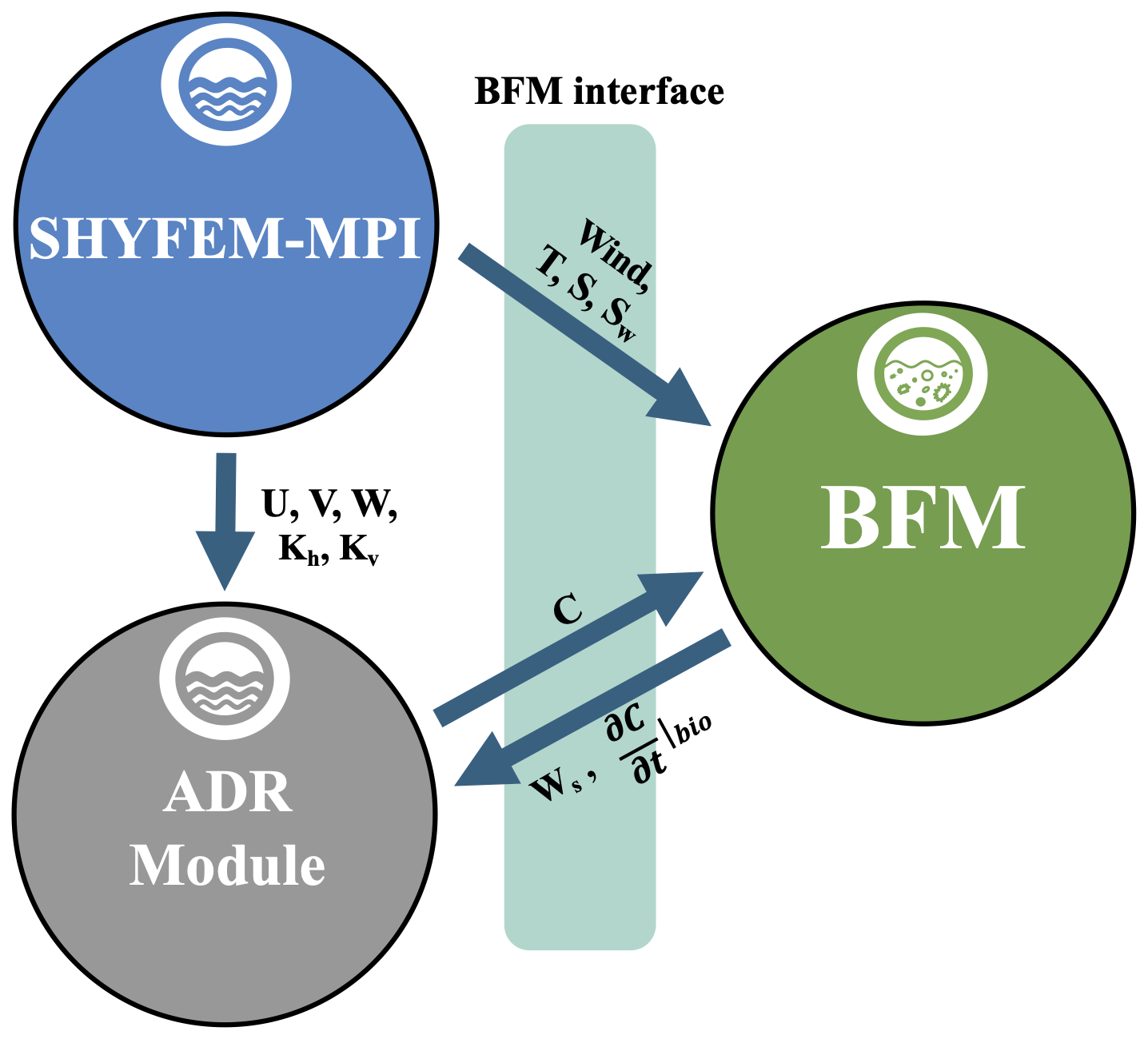
Figure 1 Scheme summarizing the coupling between SHYFEM-MPI, the ADR module and BFM, highlighting the variables that are exchanged. The interface manages the BFM specific data flow among the different components of the coupled model.

Temperature (T), salinity (S), solar radiation (S_w) and wind components are passed to BFM by SHYFEM-MPI via the BFM interface. The ADR module passes the current value of the tracer (C) to BFM that computes the rates that are then given back to the ADR module. SHYFEM-MPI provides velocity components ($U,V,W$) and the horizontal and vertical diffusion coefficient to the ADR module that solve the system to find the updated value of the tracer C. While in SHYFEM-MPI the solar radiation is computed using the MFS Bulk Formulae (Pettenuzzo et al., 2010), the possibility to provide solar radiation to BFM as an external field was added. Tracers and physical variables are initialized in both SHYFEM-MPI and BFM using data from external sources or climatological values (e.g. carbon dioxide).

3 Numerical schemes of ShyBFM

Equation (1) is numerically discretized following the formulation of SHYFEM-MPI advection diffusion equations for physical tracers (Micaletto et al., 2022) choosing an implicit time integration scheme for vertical diffusion. It is integrated over the model layer thicknesses, h_l, to allow for a better conservation in the volume since the physical model is free surface (Campin et al., 2004; Griffies et al., 2001). Therefore, the numerical form of Eq. (1) is given by:

$$\begin{array}{}\text{(11)}& \begin{array}{rl}{\displaystyle \frac{h_l^{n+\mathrm{1}}{C}_l^{n+\mathrm{1}}-h_l^n{C}_l^n}{\mathrm{\Delta }t}}& =-\left({\displaystyle \frac{\partial U_l^n{C}_l^n}{\partial x}}+{\displaystyle \frac{\partial V_l^n{C}_l^n}{\partial y}}\right)\\ & -(w_{\mathrm{t}}{C}_{\mathrm{t}}-w_{\mathrm{b}}{C}_{\mathrm{b}}{)}_l^n-(w_{S_{\mathrm{t}}}{C}_{\mathrm{t}}-w_{S_{\mathrm{b}}}{C}_{\mathrm{b}}{)}_l^n\\ & +K_{\mathrm{H}}\left({\displaystyle \frac{{\partial }^{\mathrm{2}}{h}_l^n{C}_l^n}{\partial x^{\mathrm{2}}}}+{\displaystyle \frac{{\partial }^{\mathrm{2}}{h}_l^n{C}_l^n}{\partial y^{\mathrm{2}}}}\right)\\ & +{\displaystyle \frac{\partial }{\partial z}}\left(K_{\mathrm{V}}^{n+\mathrm{1}}{\displaystyle \frac{\partial h_l^{n+\mathrm{1}}{C}_l^{n+\mathrm{1}}}{\partial z}}\right)\\ & +{\displaystyle \frac{h_l^n(\mathrm{\Delta }{C}_l^n{)}_{\text{bio}}}{\mathrm{\Delta }t}}\end{array}\end{array}$$

where the last term in the RHS is the layer-integrated biogeochemical tendency S_bgc of Eq. (1b), namely $h_l^n{S}_{\text{bgc}}=h_l^n\left(\frac{(\mathrm{\Delta }{C}_l^n{)}_{\text{bio}}}{\mathrm{\Delta }t}\right)$, while all the other terms are the discretized physical processes (S_phys). K_H and K_V are the layer-integrated discrete analogues of the horizontal and vertical diffusion coefficients (k_h, k_v). The transports are defined as:

$$\begin{array}{}\text{(12)}& U_l^n=h_l^n{u}_l^n,V_l^n=h_l^n{v}_l^n.\end{array}$$

The superscripts n and n+1 indicate the timestep at which the variables are evaluated. Subscripts t and b denote the quantities considered at the top and bottom of the layer, respectively.

Equation (1) is solved using a synchronous source splitting method (Butenschön et al., 2012), with the same timestep applied to both the “physical” and “reaction” parts. This overrides any errors arising from the use of different timesteps for different processes. The numerical scheme workflow is the following: first the biogeochemical rates (S_bgc) and the advection and horizontal diffusion terms, the latter written as $S_{\text{phys}}^{\text{expl}}$:

$$\begin{array}{}\text{(13)}& \begin{array}{rl}{S}_{\text{phys}}^{\text{expl}}& =-\left({\displaystyle \frac{\partial }{\partial x}}{U}_l^n{C}_l^n+{\displaystyle \frac{\partial }{\partial y}}{V}_l^n{C}_l^n\right)\\ & -(w_{S_{\mathrm{t}}}{C}_{\mathrm{t}}-w_{S_{\mathrm{b}}}{C}_{\mathrm{b}}{)}_l^n-(w_{\mathrm{t}}{C}_{\mathrm{t}}-w_{\mathrm{b}}{C}_{\mathrm{b}}{)}_l^n\\ & +K_{\mathrm{H}}\left({\displaystyle \frac{{\partial }^{\mathrm{2}}}{\partial x^{\mathrm{2}}}}{h}_l^n{C}_l^n+{\displaystyle \frac{{\partial }^{\mathrm{2}}}{\partial y^{\mathrm{2}}}}{h}_l^n{C}_l^n\right)\end{array}\end{array}$$

are integrated with an Euler forward scheme to give an intermediate result, ${\stackrel{\mathrm{̃}}{C}}_l^n$:

$$\begin{array}{}\text{(14)}& \begin{array}{rl}{h}_l^n{\stackrel{\mathrm{̃}}{C}}_l^n& =h_l^n{C}_l^n+S_{\text{phys}}^{\text{expl}}\left(C_l^n\right)\mathrm{\Delta }t+h_l^n{S}_{\text{bgc}}\left(C_l^n\right)\mathrm{\Delta }t\\ & +\mathrm{\Delta }t{\left[{\mathit{\delta }}_{l\mathrm{1}}{F}_{\mathrm{s}}+{\mathit{\delta }}_{lL}{F}_{\text{rem}}\left(C_{\text{bent}}\right)\right]}_l^n\end{array}\end{array}$$

where Δt is the timestep and δ is the Kronecker delta with L the index of the deepest layer of the water column and “1” indicating the first layer. The last term on the RHS of Eq. (14) accounts for the surface and bottom boundary conditions and is active only at the surface (l=1) and bottom layers (l=L). $F_{\mathrm{s}}=C_{\mathit{\eta }}(E-P-R)+R{C}_{\text{rw}}+P{C}_{\text{pw}}+F_g\left(C_{\text{air}}\right)$ is the prescribed surface flux while F_rem(C_bent) is the remineralization flux, as discussed in Sect. 2.1.

The final solution $C_l^{n+\mathrm{1}}$ is found rearranging the terms of Eq. (11) after writing the discrete form of the vertical diffusion term to give:

$$\begin{array}{}\text{(15)}& \begin{array}{rl}{\displaystyle \frac{-\mathrm{\Delta }t{K}_{\mathrm{V}(l-\mathrm{1})}^{n+\mathrm{1}}}{\mathrm{\Delta }{z}_{\text{top}\left(l\right)}}}& C_{l-\mathrm{1}}^{n+\mathrm{1}}\\ & +\left(h_l^{n+\mathrm{1}}+{\displaystyle \frac{\mathrm{\Delta }t{K}_{\mathrm{V}(l-\mathrm{1})}^{n+\mathrm{1}}}{\mathrm{\Delta }{z}_{\text{top}\left(l\right)}}}+{\displaystyle \frac{\mathrm{\Delta }t{K}_{\mathrm{V}\left(l\right)}^{n+\mathrm{1}}}{\mathrm{\Delta }{z}_{\text{bot}\left(l\right)}}}\right)C_l^{n+\mathrm{1}}\\ & -{\displaystyle \frac{\mathrm{\Delta }t{K}_{\mathrm{V}\left(l\right)}^{n+\mathrm{1}}}{\mathrm{\Delta }{z}_{\text{bot}\left(l\right)}}}{C}_{l+\mathrm{1}}^{n+\mathrm{1}}=h_l^n{\stackrel{\mathrm{̃}}{C}}_l^n\end{array}\end{array}$$

where Δz_top(l) and Δz_bot(l) are defined as:

$$\begin{array}{}\text{(16)}& \mathrm{\Delta }{z}_{\text{top}\left(l\right)}={\displaystyle \frac{h_l^{n+\mathrm{1}}+h_{l-\mathrm{1}}^{n+\mathrm{1}}}{\mathrm{2}}},\mathrm{\Delta }{z}_{\text{bot}\left(l\right)}={\displaystyle \frac{h_l^{n+\mathrm{1}}+h_{l+\mathrm{1}}^{n+\mathrm{1}}}{\mathrm{2}}}.\end{array}$$

At the surface and bottom layers, the vertical diffusive flux is not evaluated but prescribed by Eqs. (6) and (7). Accordingly, $K_{\mathrm{V}\left(\mathrm{0}\right)}^{n+\mathrm{1}}=K_{\mathrm{V}\left(L\right)}^{n+\mathrm{1}}=\mathrm{0}$ in Eq. (15), the first and last rows of the system reduce to two terms, and the prescribed fluxes enter the solution through the last term of Eq. (14).

For each node of the domain, Eq. (15) has the form of a tridiagonal matrix that is inverted using the Thomas algorithm (Thomas, 1949) to provide the final result.

4 ShyBFM testcase

The Emilia-Romagna (ER) coastal area is considered as a testing site for the ShyBFM coupled system.

Given that the physical and biogeochemical model systems have undergone extensive verification across a wide range of applications (Federico et al., 2017; Lovato et al., 2022; McKiver et al., 2016; Micaletto et al., 2022; Verri et al., 2023), no additional verification of the numerical implementation of the physical and biogeochemical processes was deemed necessary.

4.1 Emilia-Romagna coastal area

The ER coastal region (Fig. 2) is a shallow region with a maximum depth of around 50 m. The physical and biogeochemical interactions in this area are extremely important due to the presence of the Po River and other minor Apennine rivers. These form a complex network of land-borne freshwater inputs shaping the hydrological, chemical and ecological dynamics of the coastal area (Scroccaro et al., 2022; Toller et al., 2025; Zavatarelli and Pinardi, 2003). The Po River has a mean discharge of 1500 m³ s⁻¹ and a high nutrient load, accounting for over 50 % of the riverine loads discharged into the northern Adriatic Sea (Degobbis and Gilmartin, 1990; Marini and Grilli, 2023) with mean values of dissolved inorganic nitrogen (DIN; defined here as the sum of nitrate and ammonium as nitrite concentration is considered negligible), dissolved inorganic phosphorus (DIP) and reactive silicic acid (RSI) of 115.98, 2.97 and 128.29 Kt yr⁻¹ respectively (Ludwig et al., 2009) over the period 2000–2009. The variability in inorganic nutrient loads primarily drives the trophic status of the area, potentially leading to a high primary production and, in extreme cases, to severe eutrophication events resulting in hypoxic and anoxic conditions (Degobbis et al., 2000; Justić et al., 1987; Ricci et al., 2022). The northern Adriatic Sea is deeply affected by the river runoff (Scroccaro et al., 2022) and accounts for one third of the freshwater input in the Mediterranean Sea (Marini and Grilli, 2023).

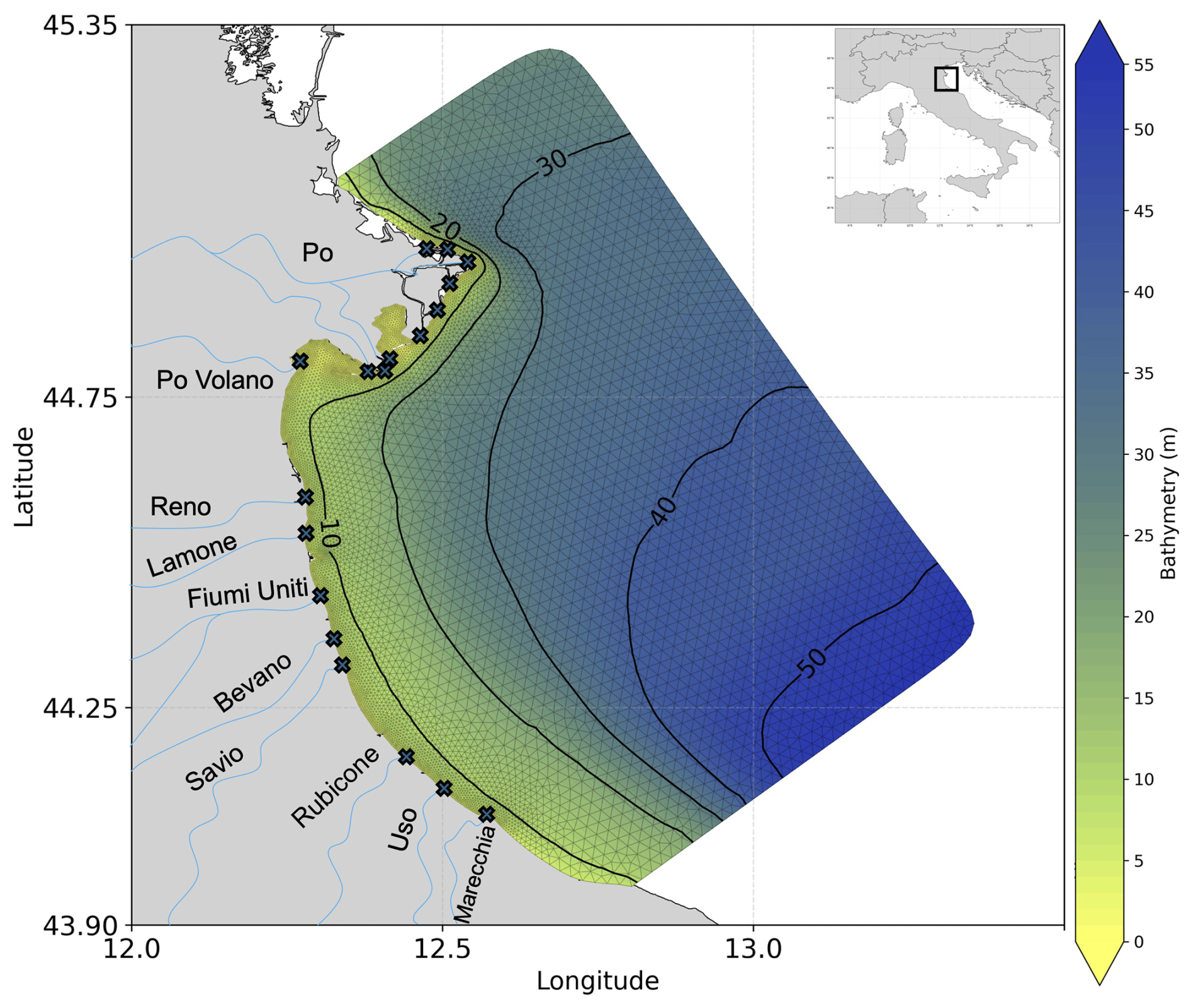
Figure 2 Testcase domain of the ER coastal area. Colours and contours indicate the bathymetry of the region. The numerical grid is superimposed in transparency. Crosses indicate the mouth of the rivers considered in the testcase. The plot in the top right corner shows the position of the domain within Italy.

The Adriatic Sea general circulation is cyclonic and a western Adriatic coastal current (WACC), driven by winds and buoyancy inputs from the Po, carries nutrient-rich water southwards. This has a significant impact across the entire Adriatic Sea (Giani et al., 2012; Ricci et al., 2022), with marked seasonal variability.

The specific domain of this study covers two ecosystem regions, classified by Mentaschi et al. (2024). These are the nutrient-rich and productive “Northern Estuarine” (NE) coastal area, influenced by river catchments (especially the Po River), and the “Northern Mesotrophic” (NM) offshore area, which has more oligotrophic conditions than the NE area but is still influenced by the hydrological forcing of the northern Adriatic. This is a well-known feature of the north-western Adriatic, characterised by a dynamic frontal system that separates low-salinity, nutrient-rich coastal waters from oligotrophic offshore waters (Jeffries and Lee, 2007; Polimene et al., 2007; Totti et al., 2019).

The abundance of nitrogen and riverine silicate input in the area leads to diatoms dominating other phytoplankton groups, limited by phosphorus availability (Knjaz et al., 2024; Vichi et al., 2003; Zavatarelli et al., 1998).

4.2 Simulation set-up

The computational model grid comprises 15 392 elements and 8142 nodes with a variable resolution ranging from 2 km offshore at the open boundary, to 300 m at the coast (Fig. 2). The vertical grid is composed of 43 z levels with 1 m thickness from the surface to 30 m depth, then increasing to 2 m up to the maximum depth of 56 m. An upwind advection scheme was chosen to avoid instabilities in solving the ADR equation for biogeochemical tracers. A higher order total variation diminishing (TVD) scheme was also tested but proved insufficiently robust due to instabilities in the biogeochemical tracers. A timestep of 200 s was chosen with a 1 h frequency output.

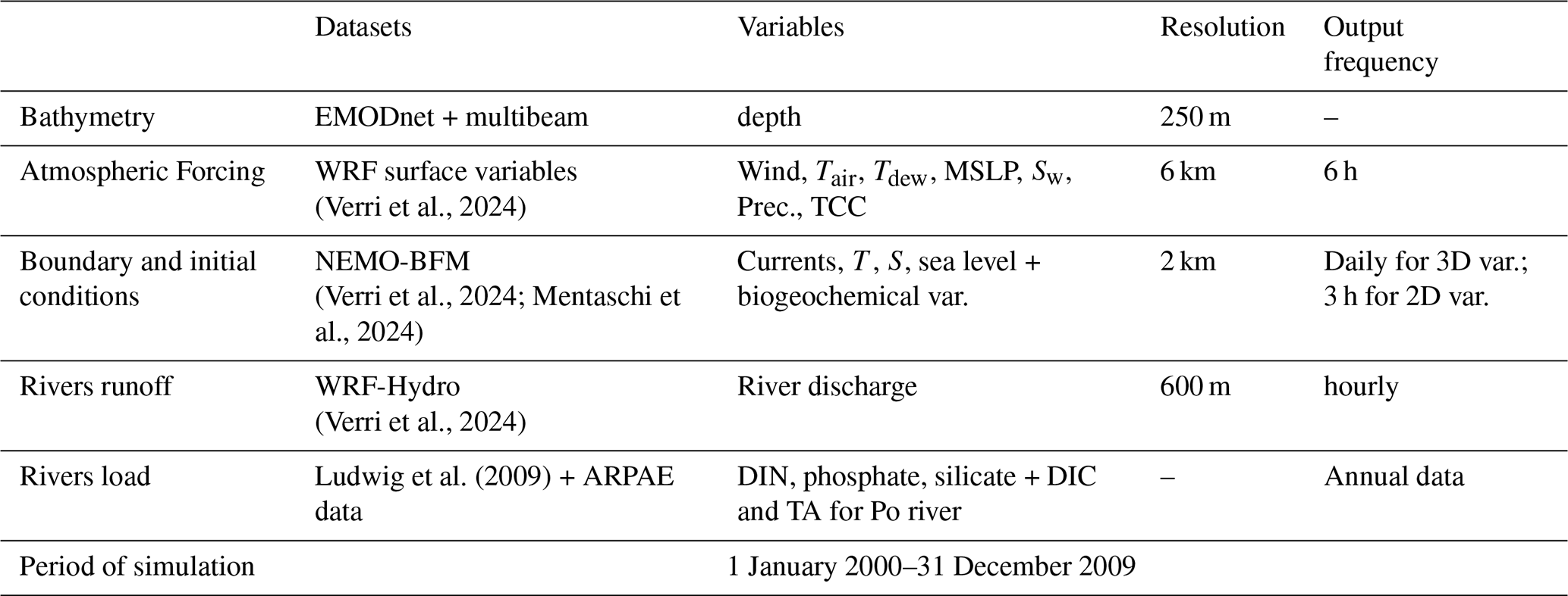
The lateral and initial conditions were provided daily (except for sea level that was provided at 3 h frequency) by a historical simulation at 2 km resolution carried out for the entire Adriatic Sea with NEMO-BFM (Mentaschi et al., 2024; Verri et al., 2024) with a vertical grid composed of 120 z levels with layer thickness going from around 1 m in the surface to more than 50 m in the deepest levels at around 2500 m. First the physical component ran with a 120 s and 2 s timestep for the baroclinic and barotropic components respectively (NEMO uses the split-explicit time stepping method), then NEMO-BFM ran offline with a 600 s timestep using NEMO-TOP (NEMO TOP WG, 2018). More details about specific model configurations are summarized in Table SI1.1 in Supplement 1 (SI 1). Tides were added to the sea level boundary condition using the TPXO tidal model (Egbert and Erofeeva, 2002). The atmospheric forcing is taken from the reconstruction of Verri et al. (2024) at 6 km resolution with the Weather Research and Forecasting (WRF) model (Skamarock and Klemp, 2008) at 6 h frequency, from which wind components, air temperature (T_air), dewpoint temperature (T_dew), mean sea level pressure (MSLP), solar radiation, precipitation and total cloud cover (TCC) are considered. River runoff was provided by Verri et al. (2024) with hourly frequency at a resolution of 600 m for the Po River and 7 other rivers in the Emilia-Romagna region (from north to south: Reno, Lamone, Fiumi Uniti, Savio, Rubicone, Uso and Marecchia in Fig. 2) using the WRF-Hydro model (Gochis et al., 2025). In addition, climatological runoff values were used for the Bevano river (Verri et al., 2018). Salinity was set to 0 for all the rivers except for the Po, where monthly values ranging from 8 to 20 psu were computed from Regional Environmental Protection Agency (ARPAE) measurements. Annual nutrient loads (DIN, phosphate and silicate) were taken from Ludwig et al. (2009) for the Po, Fiumi Uniti, Reno and Savio rivers, and values of DIN and phosphate were taken from ARPAE data (https://webbook.arpae.it/acque/acque-superficiali/, last access: 15 January 2026). Dissolved inorganic carbon (DIC) and total alkalinity (TA) data were available just for the Po River. The pre-processing procedures for the river nutrient load boundary conditions are described in Appendix A. The bathymetry of the model is derived from the 250 m resolution EMODnet bathymetry (https://EMODnet.ec.europa.eu/en/bathymetry, last access: 15 January 2026) and merged with multibeam measurements from ARPAE (https://inspire-geoportal.ec.europa.eu/srv/api/records/r_emiro:2023-06-22T141617, last access: 15 January 2026) taken along the coast up to a depth of 8 m. The simulation covers ten-years, from 1 January 2000 to 31 December 2009. Table 1 shows the simulation set-up.

Table 1 Model forcing datasets and period of simulation.

The initial configuration considered for BFM was the one implemented in Mentaschi et al. (2024), which consists of 51 pelagic variables, including 4 phytoplankton functional groups (diatoms, dinoflagellates, picophytoplankton, and large phytoplankton), 4 zooplankton functional groups (one micro-, two meso-, and heterotrophic nanoflagellates), marine bacteria, labile dissolved organic matter (DOM), and POM. It is worth mentioning that in the current implementation there is no light attenuation due to inorganic suspended matter (ISM), nor light absorption by chromophoric dissolved organic matter (CDOM), posing some limitations to ShyBFM as will be stressed in the discussion.

4.3 Model calibration

A calibration phase was performed to adjust some of the BFM model parameters over the ER coastal region. The NEMO-BFM model configuration from Mentaschi et al. (2024) was tuned for the entire Adriatic Sea. Since most of the area outside the northern Adriatic is oligotrophic, the parameters were chosen through an optimisation process that adjusted the values to be suitable for both oligotrophic and productive areas, such as the northern Adriatic Sea. In the testcase implemented here, new parameter tuning was then necessary.

The calibration for ShyBFM was carried out through a set of one-year simulations from 1 January 2000 to 31 December 2000. The dataset obtained from EMODnet (Buga et al., 2019; https://doi.org/10.6092/a8cfb472-10db-4225-9737-5a60da9af523), which contains climatological values of chlorophyll a (chl a), oxygen, DIN, phosphate and silicate for the Mediterranean Sea, was used to compare the results and tune the parameters. A list of the BFM parameters for both ShyBFM and NEMO-BFM is provided in Supplement SI 1 (Table SI1.2), highlighting the parameters that were changed compared to Mentaschi et al. (2024).

The major changes related to phytoplankton biomass rate parameters. The maximal productivity at 10 °C was increased for diatoms and dinoflagellates due to underestimation of chl a in the area. Membrane affinity for N, P and Si was also increased while minimum $\mathrm{N}/\mathrm{C}$ and $\mathrm{Si}/\mathrm{C}$ were decreased to promote phytoplankton growth at low nutrient concentrations. Moreover, the fraction of photosynthetically available radiation (PAR) was increased from 0.4 to 0.45.

Other changes related to the respiration rates of bacteria and zooplankton, which were increased due to the excess oxygen in the calibration simulations. The optimal and minimum bacterial $\mathrm{N}/\mathrm{C}$ and $\mathrm{P}/\mathrm{C}$ ratios were also slightly altered to adjust the bacterial population and the remineralization rates.

The entire calibration process required approximately 20 simulations. The final setup was then used to run a ten-year simulation, the results of which can be found in the following section.

4.4 Model evaluation

From here on, a comparison between ShyBFM, NEMO-BFM and the EMODnet climatology will be carried out and in the following sections the ShyBFM simulation will be identified as SB, the NEMO-BFM model as NB and the climatology with EMODnet.

NB represents a benchmark model and is used here to evaluate the ability of SB to correctly reproduce seasonal cycles and realistic mean values of the analysed variables, while the comparison with EMODnet provides an assessment of the model performances. In the following analysis seasons are defined by the EMODnet definition for the Mediterranean Sea (Buga et al., 2019). Winter: January, February and March; spring: April, May and June; summer: July, August and September; autumn: October, November and December.

4.4.1 Surface circulation, temperature and salinity maps

Seasonal temperature and salinity surface maps are shown in Fig. 3, where also differences against EMODnet climatology were reported.

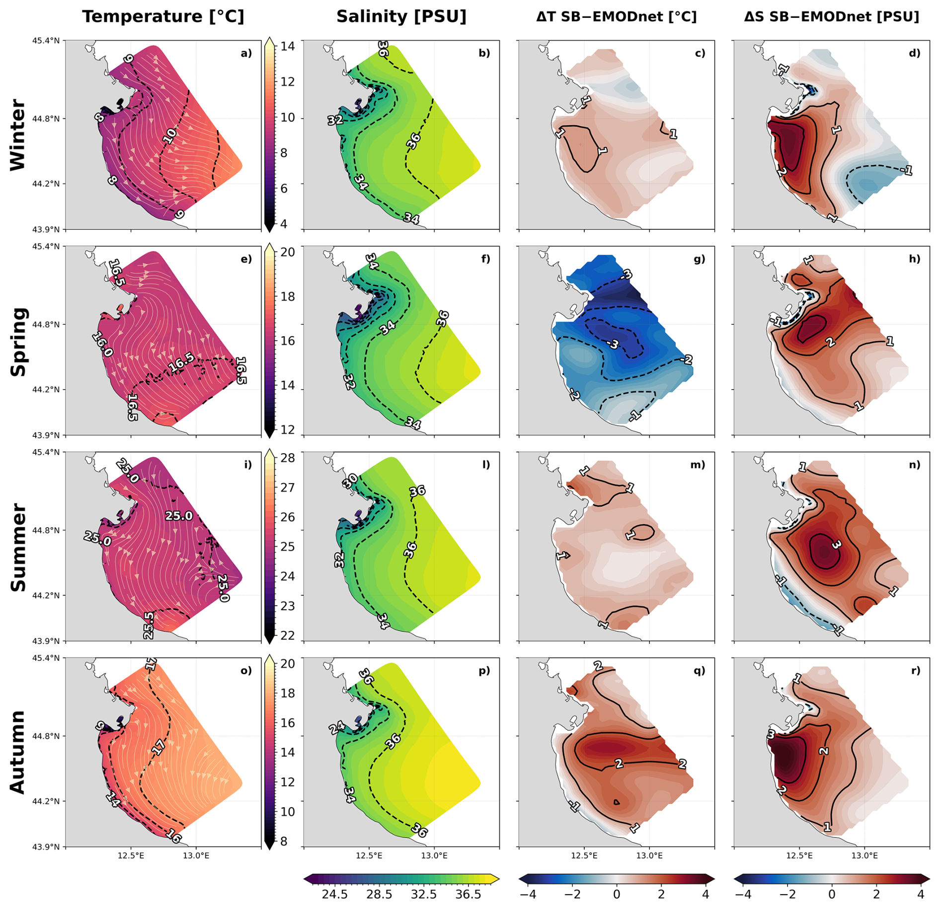
Figure 3 Seasonal surface maps of temperature with superimposed mean circulation (a, e, i, o) and salinity (b, f, l, p) for SB and differences against EMODnet climatology for temperature (c, g, m, q) and salinity (d, h, n, r).

Temperature ranges from around 8 °C in winter (Fig. 3a), along the coast, to a maximum of 25–26 °C in summer (Fig. 3i). Stronger coast-to-offshore gradients are shown in winter (Fig. 3a) and autumn (Fig. 3o), with the shallow coast being 3–4 °C colder than the offshore area. The differences against the climatology show in general a slight overestimation of temperature, except for spring (Fig. 3g), which shows temperature underestimation, with a maximum difference of more than −3 °C in front of the Po River. The maximum temperature overestimation is shown in autumn with almost 3 °C more than EMODnet in the central part of the domain (Fig. 3q).

Salinity maps show a constant sharp coast-to-offshore gradient that strengthens in spring due to increased river discharge (Fig. 3f). The salinity differences show in general two different patterns. In winter and autumn (Fig. 3d and r) the larger overestimation (more than 3 psu) is just in front of the ER coast, while in the south-east part of the domain the difference decreases or becomes even negative in winter (Fig. 3d). In spring and summer (Fig. 3h and n) the salinity is overestimated (from 1 to 3/3.5 psu) except than along the ER coast where a slight underestimation is shown (−0.5/−1 psu). Temperature and salinity maps for EMODnet climatology and NB are available in Supplement SI 2 (Figs. SI2.1 and SI2.3). The seasonal mean surface circulation is superimposed to the temperature maps (Fig. 3a, e, i, and o) to provide an indication of the circulation patterns in the area, that is mainly southward due to the wind and river forcing. Seasonal circulation maps for SB and NB and their comparison can be found in Supplement SI 2 (Fig. SI2.6). In general, both SB and NB show consistent fields of circulation, temperature, salinity.

4.4.2 Near-surface biogeochemistry

An analysis of seasonal mean near-surface (1 m depth) maps of the principal biogeochemical variables, namely chl a, DIN, phosphate, and silicate was carried out to assess the spatial patterns produced by SB (Fig. 4). The difference of SB and EMODnet is also shown (Fig. 5) by interpolating the SB fields onto the EMODnet grid. Near surface maps for EMODnet and NB, and the NB-EMODnet difference maps are provided in Supplement SI 2 for comparison (Figs. SI2.2, SI2.4, and SI2.5).

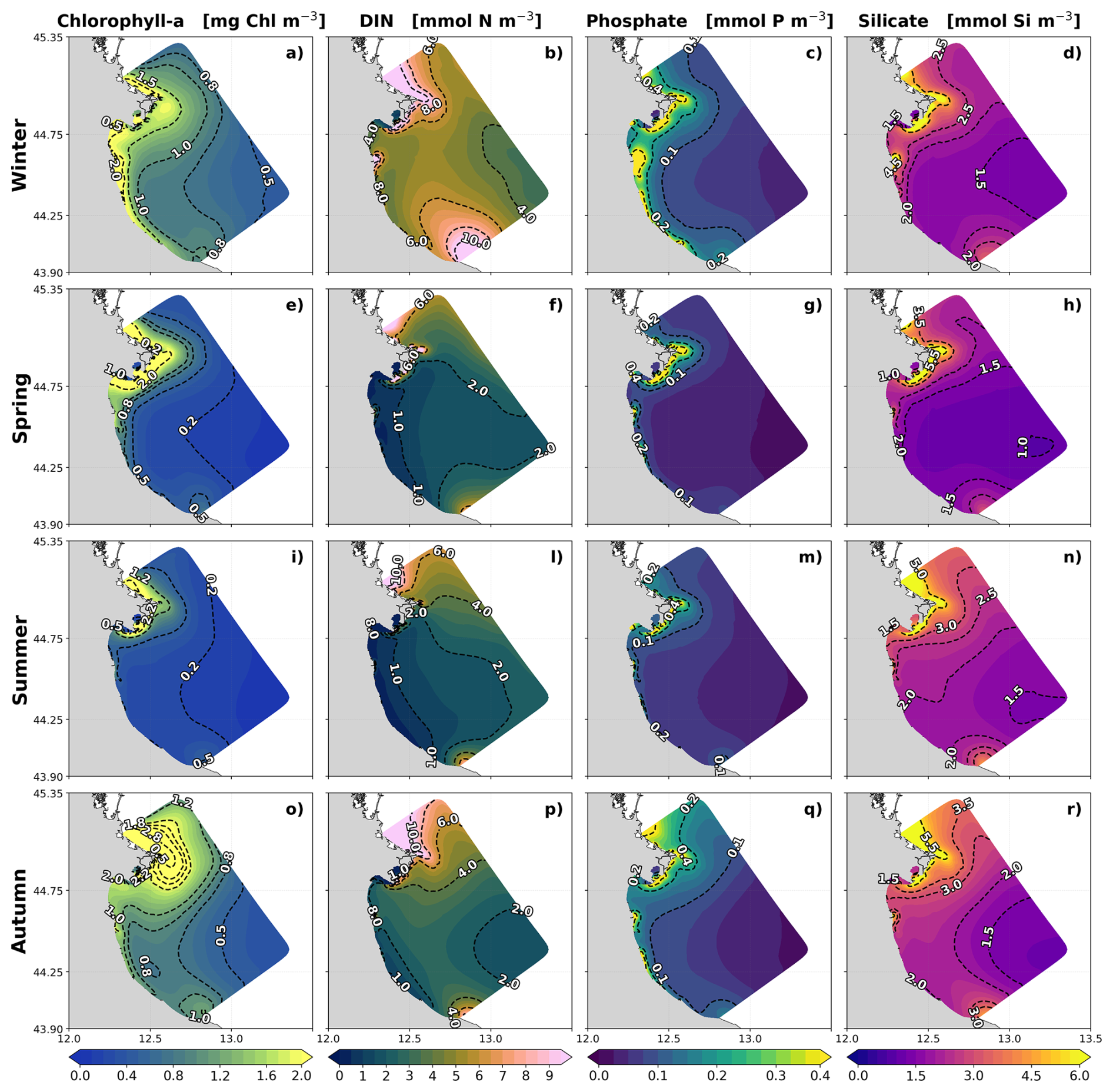
Figure 4 Seasonal near-surface spatial distribution of chl a (a, e, i, o), DIN (b, f, l,  p), phosphate (c, g, m, q) and silicate (d, h, n, r) for SB.

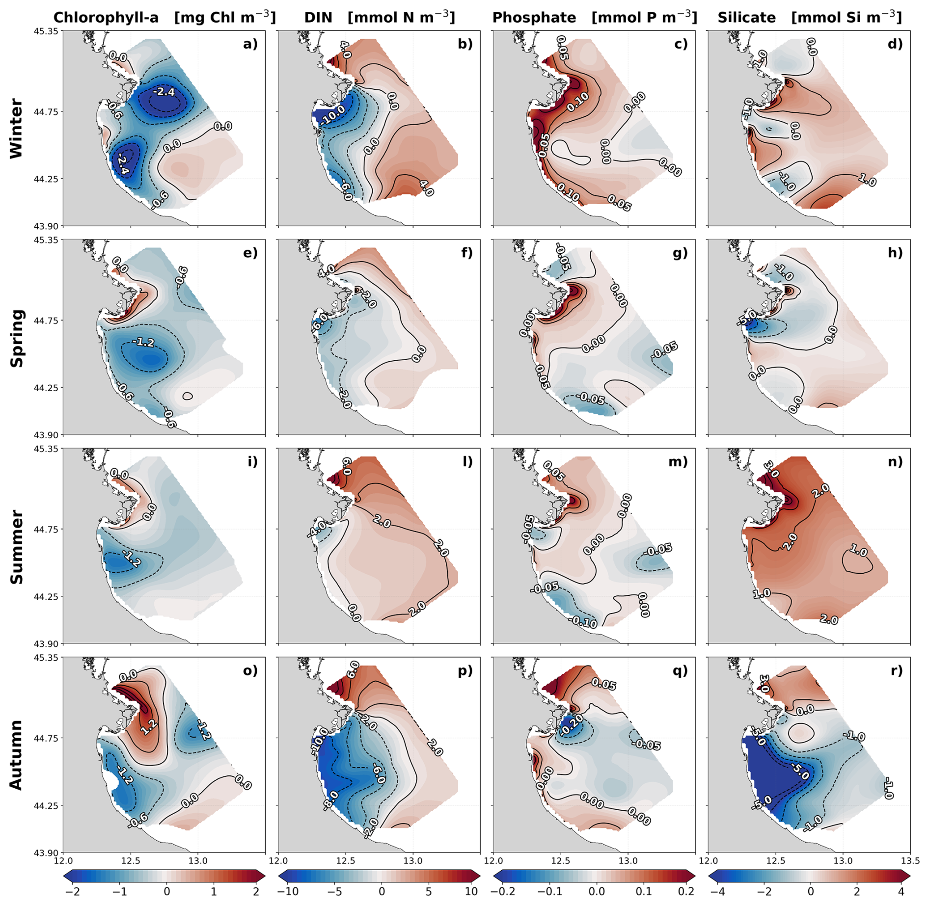
Figure 5 Seasonal near-surface differences between SB and EMODnet of chl a (a, e, i, o), DIN (b, f, l, p), phosphate (c, g, m, q) and silicate (d, h, n, r).

The patterns of chl a highlight the seasonal cycle, with maximum levels in winter (Fig. 4a, spatial median value: 1.60 mg chl m⁻³) and minimum levels in summer (Fig. 4i, spatial median value: 0.37 mg chl m⁻³). The chl a pattern follows the main southward circulation, influenced by the Po River plume and affecting the entire ER coastal area. The Po River is indeed the main source of nutrients, although other Apennine rivers (e.g. Reno, Lamone and Fiumi Uniti) also make a smaller but non-negligible contribution (Marchetti and Verna, 1992). The winter map (Fig. 5a) shows the largest underestimation of chl a reaching around −3 mg chl m⁻³ in front of the Po and along the coast. The other seasons show a positive bias around the Po mouth from 0.6 mg chl m⁻³ in summer (Fig. 5i) to a maximum of around 3 mg chl m⁻³ in autumn (Fig. 5o), while along the coast a negative bias remains from −0.6 to −1.5 mg chl m⁻³ that extends also offshore.

The DIN maps (Fig. 4b, f, l, and p) show a strong signal from the northern boundary and a weaker contribution from rivers mouth, with a maximum in winter (Fig. 4b), a spatial median value of 5.17 mmol N m⁻³ and a minimum in summer (Fig. 4l; spatial median value: 0.92 mmol N m⁻³). DIN shows a positive bias in all the seasons in the northern part of the domain and offshore with a maximum in winter (Fig. 5b) of around 15 mmol N m⁻³, while a negative bias is shown along the coast, that reach a maximum of −15 mmol N m⁻³ in autumn (Fig. 5p) south to the Po River mouth.

Phosphate (Fig. 4c, g, m, and q) shows a high seasonal and spatial variability. Higher values are found along the coast, especially at the mouth of the rivers. The highest phosphate values (spatial median value: 0.223 mmol P m⁻³) are observed in winter (Fig. 4c), which is consistent with the seasonal cycle of rivers and DIN, though a spring minimum is also observed (Fig. 4g; spatial median value: 0.082 mmol P m⁻³). Figure 5c shows a widespread overestimation of phosphate (more than 0.5 mmol P m⁻³) that occur in winter in front of the Po and along the coast. The positive bias remains in spring (Fig. 5g), although with a more limited extension. In summer and autumn (Fig. 5m and q) alternating patterns of positive and negative bias are shown, with maximum positive bias in the northern part of the domain (max 0.4 mmol P m⁻³) and a negative bias in the southern part of Po mouth (Min bias of −0.2 mmol P m⁻³ in autumn) and offshore. In front of the Reno River a positive bias is shown (0.05 and 0.1 mmol P m⁻³ in summer and autumn respectively) that in autumn extends also along the coast.

In comparison with DIN and phosphate, silicate shows a slightly less pronounced seasonal variability, with a strongly river-mouth-related spatial pattern. Surface values range from a minimum in spring (Fig. 4h; spatial median value: 1.8 mmol Si m⁻³) to a maximum in summer (Fig. 4n; 2.58 mmol Si m⁻³). In winter and spring, silicate shows positive bias in front of the Po and Reno rivers with maximum of 7 and 6 mmol Si m⁻³, respectively at rivers mouth and extending offshore, while a negative bias of around −5 mmol Si m⁻³ is shown south of the Po delta in spring (Fig. 5d and h). In summer, a widespread positive bias is shown, with a maximum of 7 mmol Si m⁻³ around the Po mouth (Fig. 5n). In autumn the maximum negative bias of −9 mmol Si m⁻³ is shown along the coast south to the Po, while a positive bias of maximum 5 mmol Si m⁻³ can be observed in the northern part of the domain (Fig. 5r).

4.4.3 Seasonal vertical profiles

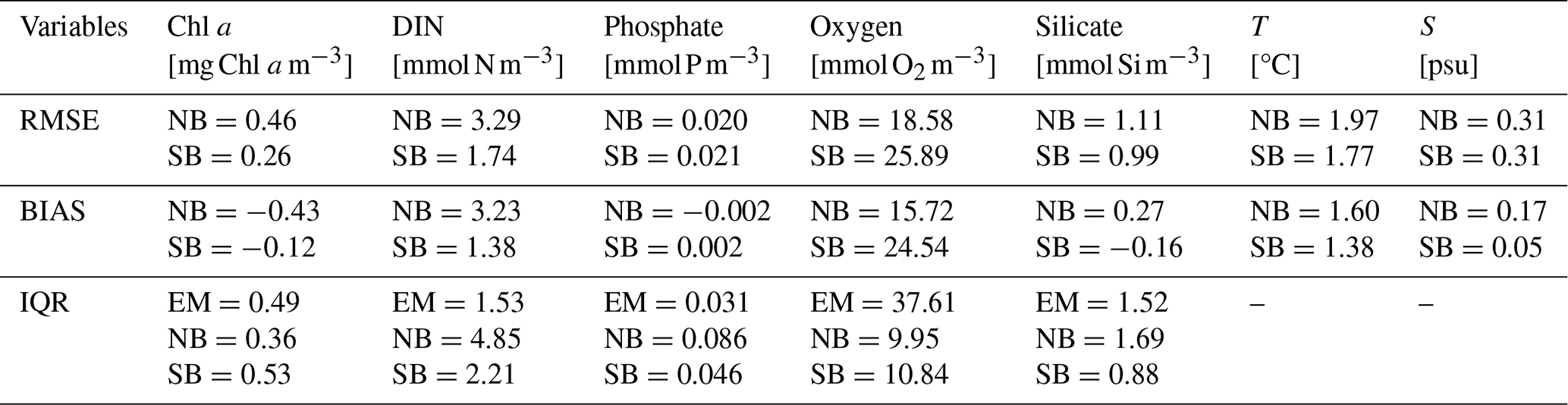
A comparison of simulated seasonal vertical profiles (from the surface down to 30 m depth) is shown in Figs. 6 and 7 for SB, NB and EMODnet for chl a, DIN, silicate, phosphate, oxygen, temperature and salinity. A summary of the performance of SB and NB against EMODnet climatology is also reported in Table 2 in terms of mean BIAS, RMSE and interquartile range (IQR). Biogeochemical variables (chl a, DIN, silicate, phosphate and oxygen) are shown with spatial median values and IQR, while temperature and salinity use mean values and standard deviation.

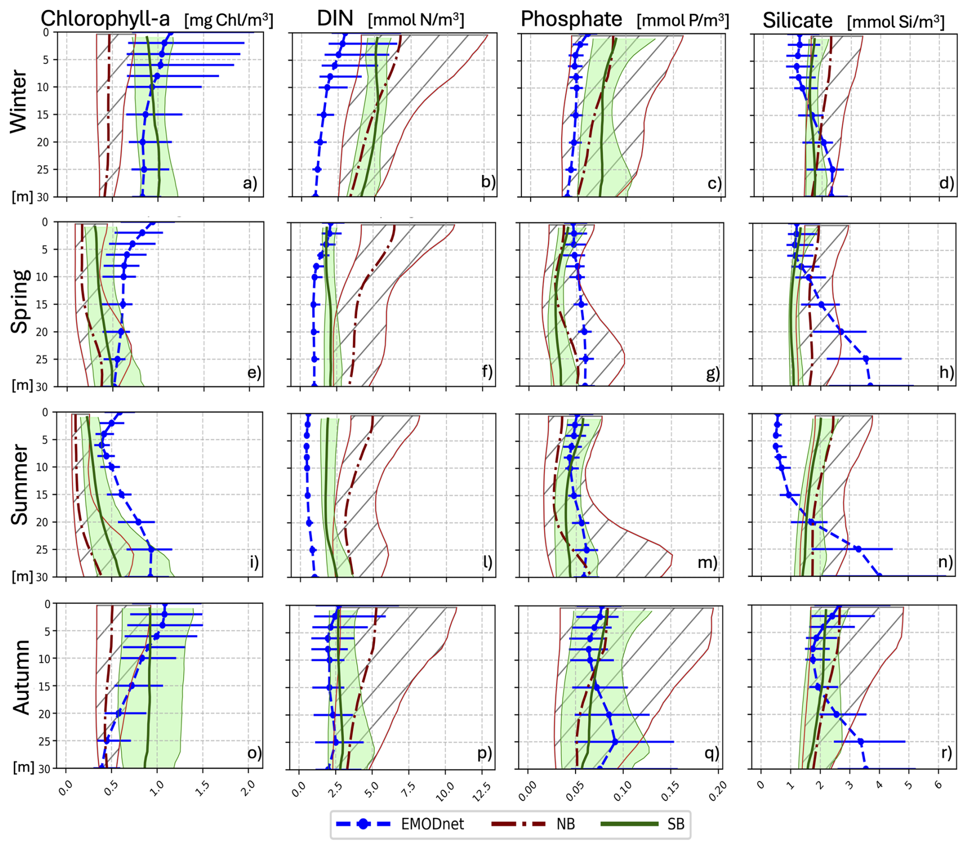
Figure 6 Seasonal spatial median vertical profiles for SB (green thick lines), NB (thick red dotted lines) and EMODnet (blue dashed lines with circles) for chl a (a, e, i, o), DIN (b, f, l, p), phosphate (c, g, m, q) and silicate (d, h, n, r). Horizontal blue bars indicate EMODnet spatial IQR, green shaded and hatched areas indicate spatial IQR for SB and NB respectively.

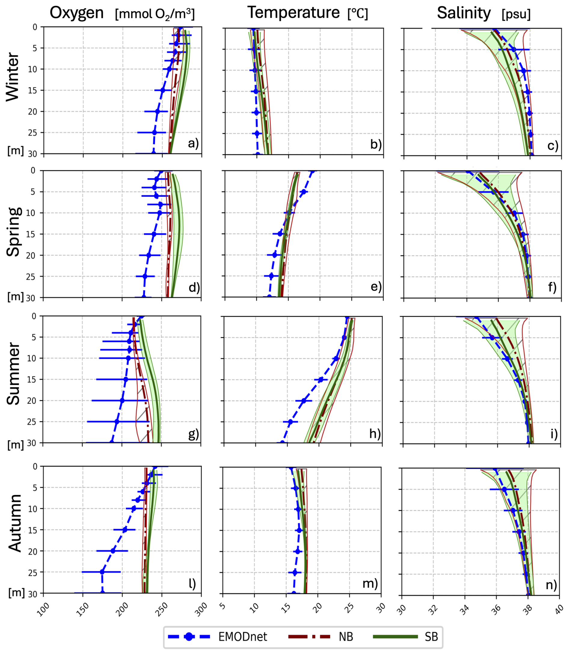
Figure 7 Seasonal spatial median vertical profiles for oxygen (a, d, g, l) and spatial mean vertical profiles for temperature (b, e, h, m) and salinity (c, f, i, n). Horizontal bars, green shaded and hatched areas indicate IQR for oxygen (left panels) and standard deviation for temperature and salinity (central and right panels).

Table 2 RMSE and BIAS averaged along the water column of temperature, salinity and a selection of biogeochemical tracers for NB and SB. The mean vertical value of IQR is also shown for biogeochemical variables of SB, NB and EMODnet (EM).

SB slightly underestimates the chl a values ($\text{BIAS}=-\mathrm{0.12}$ mg chl m⁻³) in all seasons (Fig. 6a, e, i, and o), except the lower layers in winter and autumn, but in general, SB is closer to climatology than NB. The spatial chl a variability along the water column is similar to that of NB and is well reproduced throughout the seasons, except in winter (Fig. 6a) when the climatology shows much greater variability, especially in the upper layers above 10 m depth.

DIN is overestimated (Fig. 6b, f, l, and p) in all seasons except autumn (BIAS=1.38 mmol N m⁻³), however SB shows lower DIN values compared to NB, except in the lower layers in winter (Fig. 6b). Compared to NB, SB generally shows DIN values closer to EMODnet throughout the water column, and a smaller spatial variability.

SB performance in reproducing phosphate profiles is similar to NB but there are differences between seasons. In winter, SB overestimates the climatology by around 50 % (Fig. 6c), while in spring, there is an underestimation of phosphate throughout the water column (Fig. 6g). Summer and autumn show results closer to climatology (Fig. 6m and q), with a slight overestimation in the upper layer and an underestimation below the 10–15 m depth. SB shows a lower spatial variability compared to NB that however is closer to EMODnet.

SB and NB are both unable to properly reproduce the climatological profiles of silicate (Fig. 6d, h, n, and r). The SB and NB model silicate profiles show a slight overestimation in the upper layers (between 5 and 20 m, depending on the season), while below this level, silicate is underestimated. Overall, SB performs slightly better than NB in terms of RMSE (SB=0.99 mmol Si m⁻³; NB=1.11 mmol Si m⁻³) and BIAS ($\text{SB}=-\mathrm{0.16}$ mmol Si m⁻³; NB=0.27 mmol Si m⁻³), however the spatial variability is substantially underestimated (Table 2).

As expected by air-sea equilibrium, surface oxygen is well reproduced (Fig. 7a, d, g, and l) but the performance degrades rapidly with depth. Oxygen is overestimated in all seasons for both SB and NB. Except for the surface layer, SB has a higher RMSE and BIAS compared to NB, and a slightly higher IQR (Table 2).

Temperature (Fig. 7b, e, h, and m) shows a 10 % improvement in the RMSE and a lower BIAS compared to NB, albeit the performance degrades with depth.

The salinity performance of SB is satisfactory and comparable to NB (see Fig. 7c, f, i, and n), with the best performance occurring in spring and summer, while a slight underestimation and overestimation is shown in winter and autumn, respectively. Larger discrepancies occur in the surface layers, where river runoff has a significant impact on the salinity budget.

4.4.4 Time series: interannual and seasonal cycle

As a further assessment of the testcase configuration, the median of the upper 30 m depth integrated time series of chl a, DIN, phosphate, oxygen and silicate variables for both SB and NB is shown in Fig. 8 for the simulation period. The IQR is also reported as shaded bands to illustrate daily variability. The choice to stop at 30 m depth was taken keeping in mind the purpose to focus on the coastal area.

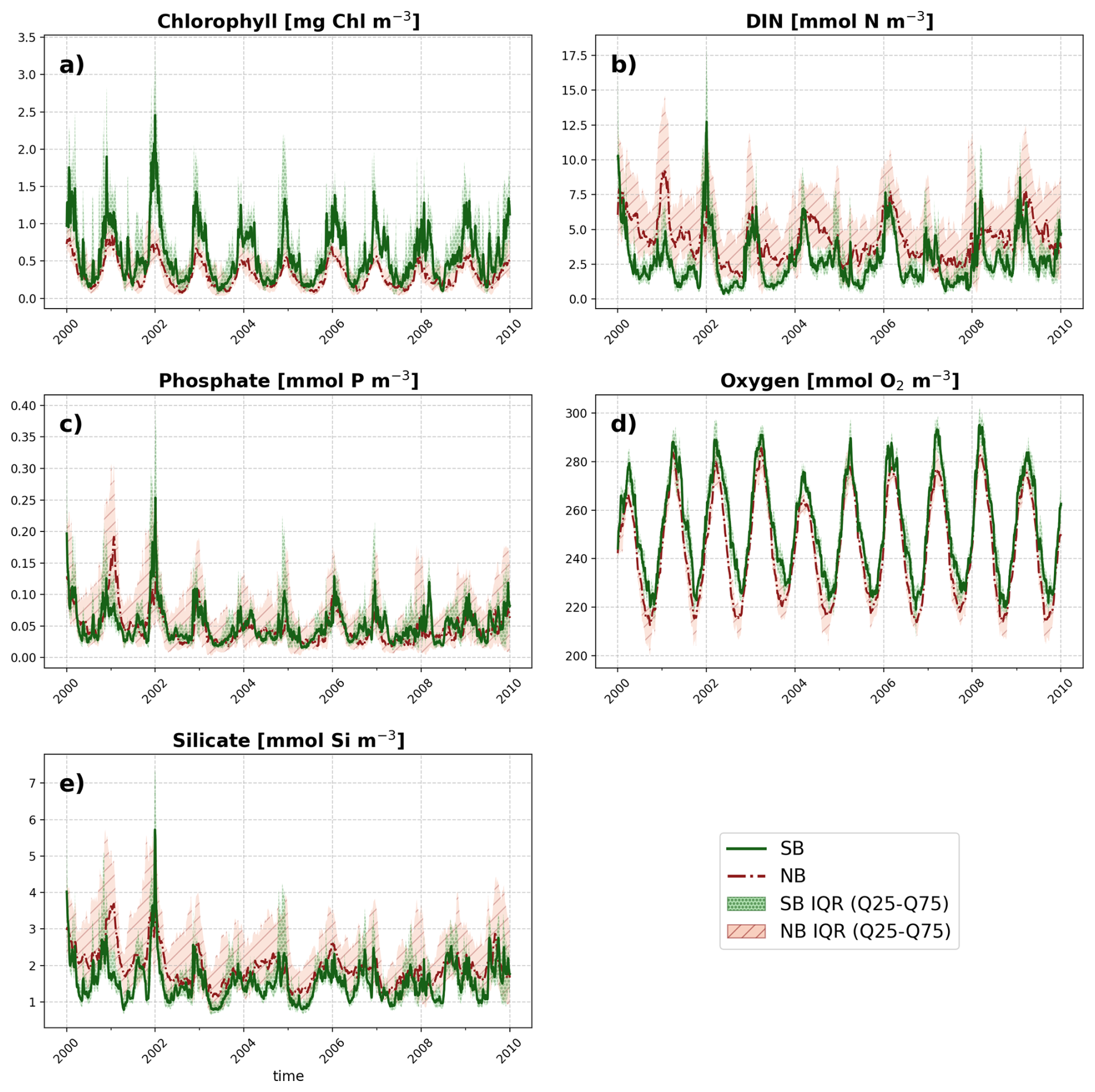
Figure 8 Daily median values for SB (green thick line) and NB (red thick dotted line), for the 10 years simulation, integrated over the domain between the surface and 30 m depth: chl a (a), DIN (b), phosphate (c), oxygen (d) and silicate (e). Light green with circles and light red hatched shaded areas indicate the spatial IQR for each modelling system, respectively.

The SB run variables analysed exhibit a seasonal signal that closely resembles that of NB. Nevertheless, the intra-monthly variability of SB is rather higher. All the variables, excluding oxygen, reached their maximum in winter 2002 (Fig. 8).

Figure 9 presents the seasonal mean boxplots of the selected biogeochemical variables for both models and EMODnet climatology. It is worth stressing that each boxplot represents spatial statistics, while seasonal values were computed as simple temporal means.

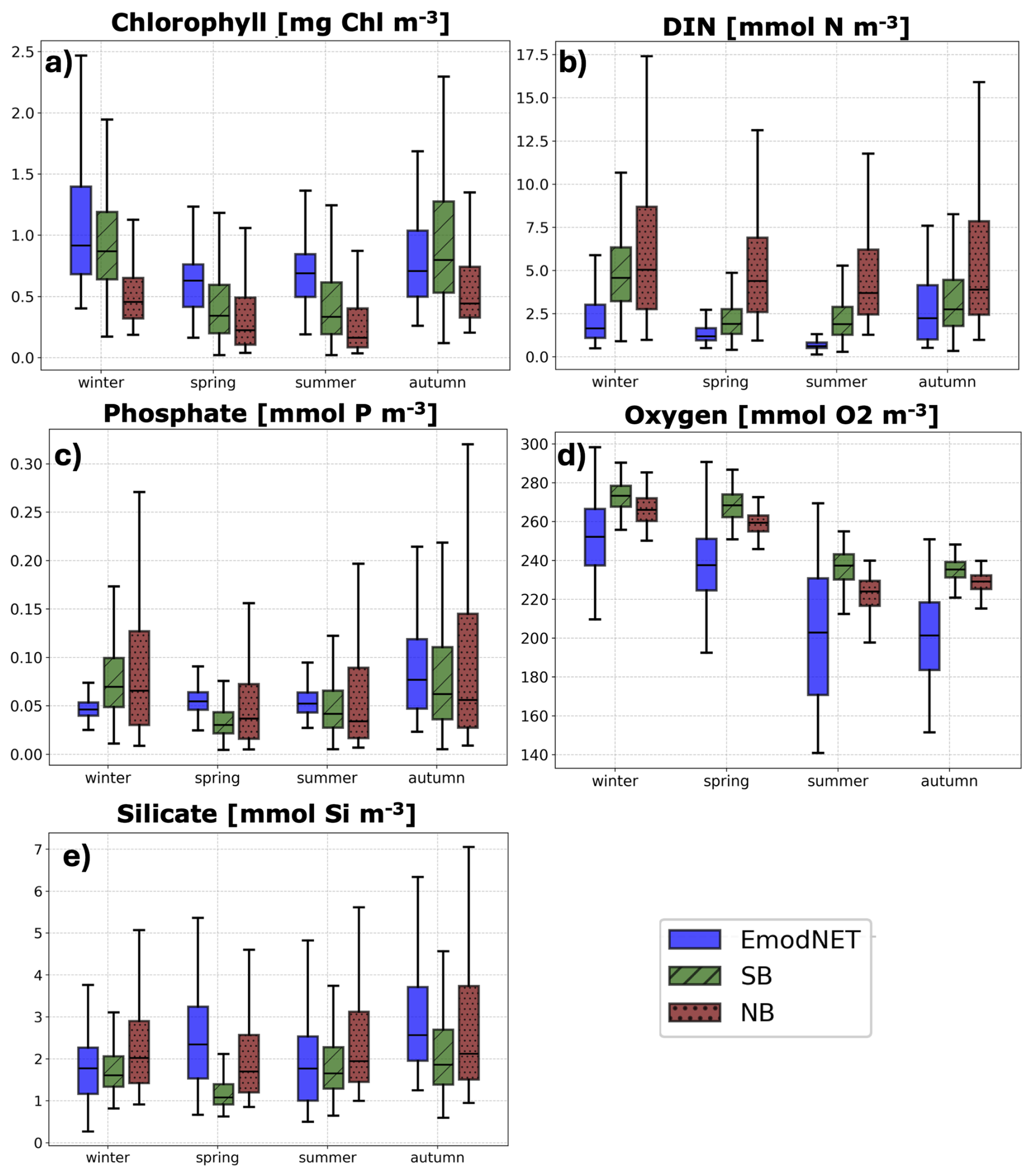
Figure 9 Boxplots indicating seasonal values of chl a (a), DIN (b), phosphate (c), oxygen (d) and silicate (e) integrated from the surface to 30 m depth for EMODnet (blue box), SB (green hatched box) and NB (red dotted box). Black line inside the box indicates the median value. The lower and upper extreme of the box represent the 1st (Q1) and 3rd (Q3) quartile respectively. Lower and upper whiskers are the minimum and maximum values found between Q1 − 1.5IQR and Q3 + 1.5IQR.

The SB chl a seasonal concentrations (Fig. 9a) are consistently higher than those of NB, particularly in late autumn and winter (Toller et al., 2025) with values generally closer to climatology. The spatial variability of chl a in SB is higher than in NB and more comparable to EMODnet, although an overestimation is evident in autumn. The SB performance for DIN is good compared to NB, especially in spring and autumn, despite a slight overestimation compared to climatology (Fig. 9b), particularly pronounced in winter. The spatial variability is lower than NB but closer to EMODnet. The SB oxygen seasonal cycle (Figs. 8d and 9d) is well represented; however, both maximum and minimum values are significantly higher than in NB and climatology (Fig. 9d). SB and NB both show a rather large underestimation of the oxygen spatial variability. The seasonal cycle of phosphate in SB closely resembles that of NB (Fig. 8c), with a slight underestimation relative to EMODnet in all seasons except winter, when both models show an overestimation (Fig. 9c). Nevertheless, the spatial variability of phosphate in SB agrees more closely with the climatology, except during winter. Silicate concentrations are slightly underestimated, especially in spring and autumn (Fig. 9e), and display lower spatial variability compared to both EMODnet and NB, although overall agreement remains satisfactory. In general, the seasonal patterns are consistent with the climatology, showing improved performance of SB for chl a and DIN, but a tendency to overestimate oxygen concentrations relative to EMODnet.

5 Discussion

Unstructured grid modelling can accurately describe complex coastal morphologies and transitional environments such as estuaries, lagoons and salt marshes, where key biogeochemical processes often occur (Bonamano et al., 2024; Cravo et al., 2024; Newton et al., 2014). This improves the representation of coastal ecosystems by enabling these environments to be included in the computational domain. The flexibility of the mesh enables changes in resolution in areas with larger spatial scales (e.g. offshore areas). Moreover, the specific parallel implementation (Micaletto et al., 2022) enables the inclusion of all 51 BFM state variables at a grid spacing of approximately 300 metres. The nested approach of ShyBFM offers flexibility in calibration of model parameters to the local areas, especially for the biogeochemical rates.

However, if not handled carefully, the limitations of unstructured grid modelling can potentially override its advantages. A discussion on the results obtained is then needed to understand the capability and limitations of SB.

Model performance

The analysis of chl a indicates the capability of SB to reproduce the phytoplankton biomass cycle, which shows bloom events between late autumn and early spring (Figs. 8a and 9a), a common feature of the northern Adriatic Sea due to the balance between light and nutrient availability and water column stratification (Vichi et al., 2003). Compared to NB chl a is well reproduced with a 45 % lower RMSE and an IQR closer to climatology (Table 2). However, there is still an overall underestimation compared to climatology, except in autumn (Fig. 9a), which shows a slight overestimation. In general, the timing of the blooming periods is consistent with the 1D modelling analysis of Vichi et al. (2003) for the area in front of the Po River. Even though the spatial variability of chl a is well reproduced, some limitations remain, particularly in the upper layers of the winter vertical profile (Fig. 6a) where the upper part of the EMODnet distribution is not well captured by the models. This discrepancy may be due both to model limitations in reproducing strong algal blooms and to inconsistencies in the data comparison, as the analysis compared a ten-year simulation (2000–2009) of SB, with a climatology spanning more than 30 years (1981–2017). It is worth noting that SB was able to reproduce two relevant phytoplankton blooms that can be noticed in 2001 and especially in 2002 (Fig. 8), during which other nutrients also exhibit consistent peaks. These events are related to the exceptionally high discharge of the Po and other rivers (Aragão et al., 2024; Verri et al., 2018), which resulted in higher nutrient loads in 2002 than the 2000–2009 mean, leading to significant mucilage events (Precali et al., 2005; Russo et al., 2005). The surface comparison of chl a with EMODnet (Fig. 5) shows similar patterns for spring, summer and autumn with a positive bias around the Po mouth and a negative bias along the coast. This pattern can be observed also in other variables of Fig. 5 and may result from uncertainties in the river nutrient loads. Other discrepancies arise from the influence of the parent model that may be strong, particularly in the northern boundary where fluxes enter the domain following the main circulation and reducing the effectiveness of domain-specific parameterizations.

The effect of nutrient fluxes entering through the northern boundary is evident in Fig. 5, especially for DIN, but also for the other variables, where larger overestimations occur in the northern part of the domain and can be attributed to the parent model (NB) due to the southward main circulation (see Fig. SI2.5 for a comparison of NB against EMODnet climatology and Fig. SI2.6 for a circulation comparison). Overall, DIN performance is good, with a 47 % reduction in RMSE compared to NB. In the final parameterization, nitrate uptake has been increased, resulting in improved agreement with climatology. However, this adjustment led to larger discrepancies with EMODnet along the coast, particularly in winter and autumn.

The phosphate performance for SB is comparable to NB. However, the IQR of SB phosphate (Fig. 9c and Table 2) is much closer to the climatology compared to NB. It is important to stress that phosphate plays a key role as a limiting nutrient in the northern Adriatic Sea, and a reliable representation of its distribution can significantly improve phytoplankton biomass equilibrium (Knjaz et al., 2024). The coupled model of Scroccaro et al. (2022) reported a substantial overestimation of phosphate in the ER coastal area, where chl a overestimation was also found, attributing this discrepancy to high uncertainty in land-borne river nutrient loads. Consistently, the comparison with EMODnet in Fig. 5 shows that the largest phosphate discrepancies occur around the Po mouth and along the coast, where several Apennine rivers discharge, supporting the role of uncertainty in river nutrient inputs. The available data enabled the computation of mean annual river load concentrations; however, actual concentrations may vary seasonally, thereby introducing additional uncertainty into the modelling framework.

Silicate results are generally satisfactory, with a 10 % reduction in RMSE (Table 2) compared to NB; however, vertical profiles (Fig. 6) show large discrepancies. The climatology indicates an increase in silicate with depth that is not reproduced by the modelling frameworks. Moreover, the IQR is underestimated by almost 50 %. The simple benthic return parameterization applied in the current model may be insufficient to represent the benthic-pelagic fluxes associated with early diagenetic processes that are particularly relevant in coastal areas (Paraska et al., 2014; Vichi et al., 2003). Silicate plays a significant role in the chlorophyll budget, as it is a fundamental component of diatom growth (Krause et al., 2019). However, silicate loads are highly uncertain due to a lack of continuous measurements. Furthermore, riverine silicate inputs are often estimated using indirect methods (Ludwig et al., 2009), which are less reliable than direct observations.

The SB model successfully reproduces the seasonal oxygen cycle (Figs. 8d and 9d), but it is affected by a systematic positive bias of 10 %–15 % (Fig. 9d). Although surface performance is good (Fig. 7), the lack of light attenuation with depth due to ISM prevents the representation of realistic vertical profiles (Zang et al., 2020). The CDOM could be also responsible for a significant fraction of light absorption (Álvarez et al., 2023; Campanelli et al., 2017) in coastal areas, but it is not considered in the configuration used here. This limitation is particularly relevant for the considered testcase, which is characterised by potentially high ISM and CDOM loads from the Po River, affecting phytoplankton photosynthetic processes (Bignami et al., 2007; Penna et al., 2004). Oxygen spatial IQR is also largely underestimated compared to climatology in both SB and NB with values that are less than one third of the climatological range (Fig. 9d and Table 2). Vichi et al. (2003) highlighted the importance of ISM in regulating phytoplankton biomass and nutrient uptake, showing that higher ISM concentrations were associated with lower chlorophyll a and higher phosphate concentrations. Both ISM and CDOM omissions likely contribute to the vertical profile discrepancies reported here. The inclusion of optical formulation accounting for CDOM (Álvarez et al., 2023) is identified as a future development. Moreover, the benthic processes may account for a large fraction of oxygen depletion in the bottom water (Seitaj et al., 2017) emphasizing the need to include benthic-pelagic coupling in coastal marine models. However, the use of more complex models should be supported by measurements of sediment variables that are lacking in the area, otherwise leading to high uncertainties in the benthic variables and their feedback to the water column. This is the main reason for the choice of a simpler benthic return closure in this first implementation of SB.

It is worth noting that in SB tides were added, which are absent in NB. Tides can reach 1 m amplitude in the northern Adriatic Sea and they can significantly enhance the mixing in water column, potentially explaining differences in stratification between SB and NB (Fig. 6).

Temperature influences phytoplankton and zooplankton growth through the metabolic (Q10) dependence in BFM, yet the temperature differences in Fig. 3 do not map onto the chl a differences in Fig. 5: the winter underestimation of chl a coincides with a slight warm bias (∼1 °C; Fig. 3c), while a much larger spring cold bias ($\sim -\mathrm{3}$ °C; Fig. 3g) leaves the chl a difference (Fig. 5e) essentially unchanged from the other seasons. This suggests that phytoplankton biomass here is controlled less by temperature than by river inputs and open-boundary conditions. Discrepancies in salinity (Fig. 3) can be attributed primarily to uncertainty in the prescribed river discharge, which sets the freshwater input and hence the strength and extent of the low-salinity plume. In addition, biases in the simulated coastal circulation, which advects the plume southward along the shelf, may displace the freshwater signal relative to observations; however, in the absence of current measurements this contribution cannot be quantified directly. SB and NB show similar temperature and salinity patterns (Fig. SI2.3) and vertical profiles (Fig. 7), indicating that these features are largely inherited from the shared forcing and boundary conditions rather than introduced by the differences in the modelling framework (grid, coupling, numerics, etc.).

The northern Adriatic coastal zone is an advection-dominated system, in which wind and river forcing govern the along-shelf transport and spread of phytoplankton biomass (Polimene et al., 2006; Zavatarelli et al., 2000). In such a regime the first-order upwind scheme adopted for horizontal advection, although robust, monotone and positivity-preserving, properties that are desirable for biogeochemical tracers, is only first-order accurate, and its diffusive truncation error tends to smooth the sharp cross-shelf and plume gradients that characterise the region, although no sensitivity experiments were carried out to isolate it from the effects of the boundary conditions, river loads or the specific choice of biogeochemical parameters. Nevertheless, a higher-order advection scheme would be expected to improve the simulated spatial patterns and is left for future work.

Pelagic remineralization rates driven by bacterial activity also play a crucial role in coastal waters (Nixon, 1981) and were the focus of part of the calibration phase, with significant impacts in oxygen and inorganic nutrient concentrations. However, no reference data were available for direct comparison with modelled bacterial biomass.

Overall, the results demonstrate the ability of SB to reproduce the physical and biogeochemical cycles of the testcase area with promising results when implemented accurately with specific parameter calibration and output validation. SB outputs are comparable to those of NB, which serves as the benchmark model, and for several variables, SB shows improved performance relative to the climatology.

In terms of computational cost, SB required around 695 core-hours per simulated year with 36 MPI processes, while NB used around 1728 core-hours per simulated year with 288 MPI processes. This means a wall clock of around 19 h for SB and 6 h for NB per simulated year. NB was almost 3 times faster but used around 2.5 times more core-hours compared to SB.

6 Conclusions

In this study, a new coupled model, ShyBFM v1.0, is presented. The system consists of the SHYFEM-MPI ocean model and the BFM biogeochemical model, coupled through a dedicated numerical implementation of the ADR equation. The numerical solution adopts a synchronous source splitting technique for biogeochemical rates and an implicit formulation for the tracer time stepping.

SB has been implemented in the coastal area of the Emilia-Romagna region in the northern Adriatic Sea, a dynamically complex environment characterised by large nutrient inputs from the Po River. The nested approach provides considerable flexibility in representing coastal processes across scales, using higher resolution and a more focused calibration. A large number of sensitivity experiments were performed to calibrate biogeochemical parameters, particularly those related to living functional groups. A ten-year simulation (2000–2009) was then conducted, and results were compared with those of the nesting model NB and EMODnet climatology.

The results demonstrate the ability of SB to reproduce the expected biogeochemical cycles (chl a, DIN, phosphate, silicate), improving upon or matching the performance of NB in most cases. An overestimation of oxygen concentration was identified, possibly linked to the absence of CDOM and sediment-induced light attenuation along the water column. As observed in many coastal systems, strong spatial gradients in temperature, chlorophyll and dissolved nutrients make empirical parameterizations particularly challenging (Peña et al., 2010; Ward et al., 2025). Future calibration strategies based on machine learning approaches could help explore parameter space more efficiently and improve local biogeochemical model performance (Buchanan et al., 2025).

Despite the uncertainties concerning empirical parameter calibration and river nutrient load estimates, the performance of SB is satisfactory. However, several limitations remain to be addressed. Low-order advection schemes potentially introduce numerical diffusion, and the simplified benthic return parameterization does not resolve complex early diagenetic processes in shallow environments but was currently the most consistent choice for this first implementation. Future developments should incorporate higher-order advection schemes, the inclusion of ISM and CDOM for light absorption and more mechanistic sediment diagenetic modules, building on the unstructured framework, which already resolves the complex coastal geometry and cross-shelf gradients at variable resolution.

Reducing uncertainties in coastal biogeochemical modelling also requires improvements in external forcing and in local observational networks: finer, kilometre-scale downscaling would better resolve coastal winds and air-sea fluxes at very high resolution, but is computationally very expensive (Denamiel et al., 2021), while denser in-situ networks are needed to better constrain river nutrient loads and boundary conditions. A higher frequency of river nutrient loads measurements would be of great benefit to generate a more consistent forcing and reduce uncertainty.

Overall, ShyBFM v1.0 represents a promising tool for high-fidelity coastal biogeochemical modelling, combining mesh flexibility, full baroclinicity and a detailed representation of the lower trophic ecosystem dynamics.

Appendix A

The inorganic nutrients from rivers are described in terms of dissolved inorganic nitrogen (DIN), dissolved inorganic phosphorus (DIP) and silicates (SiO4) and are provided by EMODnet in the framework of the PERSEUS project (https://EMODnet.ec.europa.eu/en/river-inputs-4, last access: 20 December 2025) on an annual basis. Among the Emilia-Romagna rivers, EMODnet provides data for the Po River, Reno River, Fiumi Uniti and Savio. To test the nutrients loads of rivers in the coupled ShyBFM model, the total amount of DIN was considered as nitrate and the total amount of DIP as phosphate. The rivers are thus represented as a source of nitrate, phosphate and silicate. The data provided are given as a mass flow rate in kt yr⁻¹. However, SHYFEM-MPI needs data as a concentration in mmol m⁻³. The first step is to convert data from kt yr⁻¹ to mmol s⁻¹. The conversion is carried out using the tracers molar mass (MM). The conversion from mass flow rate, FR_mass (kt yr⁻¹) to a molar flow rate, FR_mols (mmol s⁻¹) read:

$$\begin{array}{}\text{(A1)}& {\text{FR}}_{\text{mols}}={\displaystyle \frac{K{\text{FR}}_{\text{mass}}}{\text{MM}}}\end{array}$$

where K is a conversion coefficient that accounts for the conversion from kt to mg (km=10¹²) and from year to seconds ($\text{tc}=\mathrm{31.536}\times {\mathrm{10}}^{\mathrm{6}}$ s yr⁻¹, for a non-leap year) so that $K=\frac{\text{km}}{\text{tc}}$.

The final conversion to a concentration C_rw (mmol m⁻³) is carried out using the mean runoff of the rivers, $\stackrel{\mathrm{‾}}{D}$ in m³ s⁻¹. Eventually the annual concentration value C_rw is found as:

$$\begin{array}{}\text{(A2)}& C_{\text{rw}}={\displaystyle \frac{{\text{FR}}_{\text{mols}}}{\stackrel{\mathrm{‾}}{D}}}.\end{array}$$

The concentration C_rw is provided to SHYFEM-MPI as a vertical boundary condition (Eq. 6) as discussed in Sect. 2.1. This implies that the mean river runoff $\stackrel{\mathrm{‾}}{D}$ used to compute C_rw should be consistent with the river runoff R prescribed in Eq. (6).

Appendix B: Definition of terms

Symbol	Description
$C(x,y,z,t)$	Generic tracer concentration
$C_{\mathit{\eta }}(x,y,t)$	Tracer concentration at sea surface
$C_{\text{rw}}(x,y,t)$	Tracer concentration at river boundary
$C_{\text{pw}}(x,y,t)$	Tracer concentration in precipitation
$C_{\text{bent}}(x,y,t)$	Tracer areal content in the benthic compartment
$C_{\text{air}}(x,y,t)$	Tracer concentration in the atmosphere
Cext	Tracer imposed at the lateral boundary
Cint	Tracer concentration of the nearest interior point
Fg(Cair)	Dry deposition flux at air-sea interface
t	Time variable
$(x,y,z)$	Cartesian grid coordinates in the zonal, meridional and vertical directions
H	Bottom depth
∇h	Horizontal gradient operator
uh	Horizontal water velocity
w	Vertical water velocity
ws	Settling material velocity, positive upward
kh	Horizontal diffusion coefficient
kv	Vertical diffusion coefficient
η	Sea surface height referred to model coastline
hl	Thickness of layer “l”
E	Evaporation
P	Precipitation
R	Run off
V	Total volume of the domain
Ω	Area of the domain
Fs	Surface fluxes
Frem(Cbent)	Remineralization flux