Effectively assimilate satellite land surface temperature into offline land surface models within ensemble-based assimilation frameworks

Land surface temperature (LST) plays a vital role in controlling the water and energy fluxes at the interface between the land and atmosphere, and the main aim of assimilating LST observations into Land Surface Models (LSMs) is to not only provide better initial conditions for the LSM itself, but also yield more accurate land–atmosphere interactions. While observation systems provide a vast amount of satellite-derived LST observations in recent years, they are not as widely used as soil-moisture observations in land data assimilation (DA), in research or in operations, owing to the fast temporally varying nature of LST. This study proposes a new scheme to effectively improve the impact of LST assimilation by simultaneously updating soil temperature and soil moisture within the upper soil layers. The proposed scheme outperforms the conventional strategy of updating temperature only, and it also yields significant benefits for hydrological variables such as soil moisture and snow. The DA method and LSM used in this study are the Local Ensemble Transform Kalman Filter (LETKF) and the Common Land Model (CoLM), respectively. Moderate Resolution Imaging Spectroradiometer (MODIS) derived LST is assimilated into CoLM every 3 h using the proposed scheme. The assimilation and open-loop experiments are conducted for one year with a global resolution of 0.5°×0.5°. The LST shows marginal enhancement after assimilation, owing to its fast-varying nature dominated by atmospheric forcings. However, the BIAS in soil temperature over Northeast Asia is reduced significantly, with a magnitude of 1.0, 1.5, and 2.0 K for the layers within 0–10, 40–100, and 100–200 cm, respectively. Prominent improvements in snow temperature and snow depth are observed over Northeast Asia, with a reduction in root mean square difference (RMSD) of approximately 4 K and 150 mm, respectively. The improvements in soil water content are also notable, particularly over humid tropical regions. The largest reductions in unbiased RMSD of soil water content over the Amazon Rainforest are approximately 0.06, 0.12, 0.15, and 6.00 kg m⁻² for the layers within 0–10, 10–40, 40–100, and 100–200 cm, respectively. These consistent improvements in both the energy and water components of CoLM demonstrate the effectiveness of the proposed scheme and the importance of LST assimilation for land-surface-process modeling.

1 Introduction

Land surface temperature (LST) is defined as a Global Climate Observing System Essential Climate Variable for its irreplaceable value in assessing both the land-atmosphere interaction and the land surface process itself (Global Climate Observing System, 2022). Through soil moisture and LST, understanding of the land surface process from a climatic perspective has made significant progress in the last few decades (Jin and Dickinson, 2002; Kalnay and Cai, 2003; Seneviratne et al., 2010). To a large extent, this progress can be seen as a result of the rapid development of satellite-based observations at the land surface, which provide much broader spatial coverage than ground-based measurements and yield supplementary information for regions with few in situ observations (De Lannoy et al., 2022). These newly emerging remote sensing observations have gained popularity in the field of land and hydrologic data assimilation (DA) (McLaughlin, 1995; Swinbank et al., 2003; Reichle, 2008; Khaki et al., 2020; Zafarmomen et al., 2024). Together with the conventional observations, remote sensing observations have been assimilated into Land Surface Models (LSMs) in many operational centers worldwide (Rodell et al., 2004; Balsamo et al., 2007; Drusch, 2007).

For the long memory (Vinnikov et al., 1996; Koster and Suarez, 2001) and continuous influence of the land surface on the atmosphere, which is somewhat comparable to the sea-atmosphere interaction (Koster et al., 2000, 2004), satellite-based soil moisture has been assimilated into several LSMs and led to significant improvements in both operational and research contexts (Reichle et al., 2002; Crow and Wood, 2003; De Rosnay et al., 2013, 2014; Muñoz-Sabater et al., 2019; Bonan et al., 2020). In the land DA community, the variables directly associated with the atmosphere such as evaporation (Meng et al., 2009) or LST itself (Bosilovich et al., 2007), rather than the variables within the upper soil layers such as soil temperature and moisture, are updated when assimilating LST. This preference is a consequence of the extremely volatile energy stored in the upper soil layers, which is strongly controlled by the incoming solar radiation and outgoing thermal radiation. Therefore, it seems to be more effective to assimilate LST into the atmosphere through land-atmosphere interaction. While assimilating LST into atmosphere could be easily achieved in a coupled model, where the interaction between land and atmosphere is bidirectional (Browne et al., 2019; Zhang et al., 2020), it is not applicable in an offline LSM, where the atmosphere only acts as boundary conditions for the land surface.

Based on the offline Common Land Model version 3.0 (CoLM, Dai et al., 2003) and the Ensemble Kalman Filter (EnKF, Evensen, 1994; Burgers et al., 1998; Evensen, 2003), a one-dimensional land DA scheme was designed to update the soil temperature profile on sites by assimilating LST (Huang et al., 2008). Through a simple observation operator based on the linear relationship between LST and in situ ground temperature, the assimilation results exhibited significant enhancements over the open loop (i.e., without DA). This improvement stemmed primarily from utilizing LST to update soil temperature encompassing both the upper and the deeper soil layers, as the deeper soil layers prevent the adjusted energy from being quickly dissipated and therefore keep the impact longer than the upper ones. Although the main motivation of this early study was to demonstrate the potential of assimilating remote sensing observations into the CoLM using the EnKF, it is noteworthy that directly using LST to update the soil temperature profile may not be physically plausible. This is because the influence of LST is typically limited to the surface and does not extend to a significant depth (Jin and Dickinson, 2010). Despite other attempts to assimilate LST into offline LSMs, such as storing its impact within the soil water content (Lakshmi, 2000) or employing a bias correction method before performing DA (Bosilovich et al., 2007; Reichle et al., 2010), the question of how to effectively assimilate LST into LSMs remains open in an offline context.

Following the work by Huang et al. (2008), Chen et al. (2021) assimilated brightness temperature to update soil moisture and LST to update soil temperature, respectively, into the CoLM using the EnKF with an observation operator based on physics. The updated states are also influenced by distant observations, which helps to mitigate spatial discontinuities in the analysis increments. Although the improvements are prominent in both soil moisture and temperature when assimilating multi-source remote sensing measurements, it is challenging to distinguish the contribution of LST among the different observations.

The aforementioned studies demonstrate the promising benefits of assimilating LST into LSMs; however, their assimilation strategies are limited to updating individual states separately. Specifically, Huang et al. (2008) assimilated LST to update only the soil temperature profile, whereas Chen et al. (2021) assimilated LST and brightness temperature separately to update soil temperature and soil moisture, respectively. Initially, assimilating LST to update only soil temperature yielded marginal improvements because the surface thermal memory is rapidly lost as the state relaxes back to the trajectory dictated by atmospheric forcing. Therefore, a joint update of soil temperature and soil moisture in the top two layers was introduced, revealing a promising improvement (Fig. 1). In addition, the joint update also improves snow-related variables notably compared with updating only soil temperature (results not shown here). By jointly updating these variables, the persistent memory of soil moisture and the thermal inertia of soil temperature are leveraged to sustain the post-assimilation impact. Although soil moisture is not explicitly used in the LST observation operator (see Sect. 2.2), this joint update can be achieved implicitly within an ensemble-based assimilation framework via the background error covariance between soil water content and soil temperature (see Sect. 2.3). Hence, this paper proposes jointly updating soil temperature and soil moisture when assimilating LST in an offline land surface model within an ensemble framework, and systematically evaluates the assimilation performance.

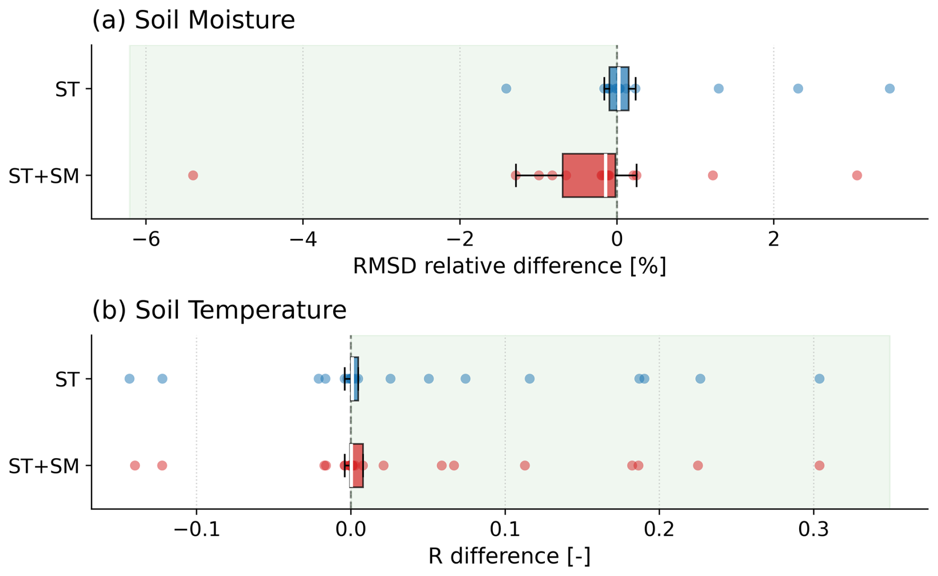
Figure 1 Comparison of assimilation performance between the joint-update (ST+SM) and temperature-only (ST) schemes across AmeriFlux sites. Panel (a) shows the RMSD relative difference (%) for soil moisture. Panel (b) shows the correlation coefficient (R) difference for soil temperature.

The land DA has evolved from incorporating near-surface meteorological observations to initialize soil moisture in LSMs (Mahfouf, 1991), to assimilating brightness temperature to update soil profile properties by solving the inverse problem with the Extended Kalman Filter (Entekhabi et al., 1994), and to assimilating brightness temperature with the EnKF (Crow and Wood, 2003). This study adopts the Local Ensemble Transform Kalman Filter (LETKF, Hunt et al., 2007) for its ease of implementation and high degree of parallelism. The LETKF has been widely utilized in atmospheric research (Bonavita et al., 2010) and operational settings (Miyoshi et al., 2010; Hamrud et al., 2015), and it has been applied to several LSMs for land studies (Han et al., 2014; Seo et al., 2021; Kurosawa et al., 2023). The LST retrieved from the Moderate Resolution Imaging Spectroradiometer (MODIS) is used in this study for its robust quality (Pérez-Planells and Martin, 2020) and extensive applications to LSMs (Yu et al., 2014; Fu et al., 2020; Huang et al., 2008).

This paper demonstrates jointly updating soil temperature and moisture to effectively assimilate LST into offline land surface models within ensemble-based assimilation frameworks. Section 2 briefly introduces the CoLM, the LST observation operator and the LETKF method. Section 3 describes the atmospheric forcing, the LST observations, the validation datasets, and the experimental design. Comprehensive evaluations of the performance of LST assimilation are presented in Sect. 4. Section 5 discusses the issues encountered in this study and gives prospects. Finally, Sect. 6 gives the conclusions of this study.

2 Methods

2.1 CoLM Configuration and Ensemble Generation

CoLM was developed by a collaborative effort of scientists with the conception of a modular LSM for weather prediction and climate research (Dai et al., 2003). It incorporates the most advantageous features of three well-documented and exceptional LSMs (Bonan, 1996; Dickinson et al., 1993; Dai and Zeng, 1997), and its technical details are well documented (Ji and Dai, 2010). It has undergone critical improvements over the original version in various aspects, among which the most notable feature is the two-big-leaf scheme, making more accurate representation of the leaf temperature possible (Dai et al., 2004). The specific version used in this study is from the offline component of the GRAPES (Global/Regional Assimilation and Prediction Enhanced System) model at the China Meteorological Administration, and it is developed based on CoLM 2014.

It comprises one vegetation layer, 10 soil layers with thicknesses of 0.018, 0.028, 0.045, 0.075, 0.124, 0.204, 0.336, 0.554, 0.913, and 1.137 m, and dynamic snow layers with levels up to 5. The vertical layer index l is from −4 to 10 with $-\mathrm{4}\le l\le \mathrm{0}$ for snow layers and $\mathrm{1}\le l\le \mathrm{10}$ for soil layers. CoLM adopts the concept of mosaic (Avissar, 1992; Koster and Suarez, 1992), allowing each model grid cell to be subdivided into different patches, each for a unique land cover type.

CoLM's integration accounts for both energy and water processes, with theoretical details provided in Dai et al. (2003) and implementation specifics outlined in Ji and Dai (2010). In this study, the state variables updated by DA include sunlit leaf temperature (T_lsun) and shaded leaf temperature (T_lsha) in the canopy; ground temperature (T_g, temperature at the top valid layer); soil temperature (T_l), soil liquid water ($W_l^{\text{liq}}$), and soil solid water ($W_l^{\text{ice}}$) within the top two valid layers ($l_{\text{top}}\le l\le l_{\text{top}}+\mathrm{1}$) – these soil variables are updated simultaneously. When snow is present, snow temperature and water/ice content are updated analogously. The index of the top valid layer l_top=1 if no snowpack was accumulated above the ground, otherwise l_top=l, where l is the first layer (starting from −4 to 0) for which $W_l^{\text{liq}}+W_l^{\text{ice}}>\mathrm{0}$.

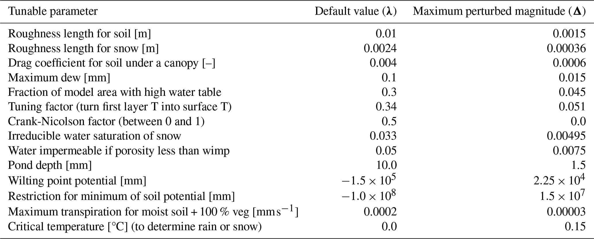
For the assimilation experiment, 14 tunable parameters (Table 1) in the CoLM are perturbed as follows to account for model uncertainty, which is vital for maintaining a realistic ensemble spread.

$$\begin{array}{}\text{(1)}& {\stackrel{\mathrm{̃}}{\mathit{\lambda }}}_k=\mathit{\lambda }+r_k\mathbf{\Delta },k=\mathrm{1},\mathrm{2},\mathrm{\cdots },K,\end{array}$$

where K and r_k are the number of ensemble members and a random number drawn from a uniform distribution $U(-\mathrm{1},\mathrm{1})$ for the kth ensemble member; λ and Δ are the vectors of the default values (the 2nd column in Table 1) and the maximum perturbed magnitudes (the 3rd column in Table 1) of the tunable parameters, respectively. The random factor r_k is re-sampled at the beginning of each assimilation cycle for each ensemble member to represent time-varying model uncertainty. This perturbation scheme maintains a realistic ensemble spread while preserving the model's intrinsic water and energy balance, as confirmed by preliminary diagnostic tests.

Table 1 Tunable parameters, their default values and maximum perturbed magnitudes in CoLM.

2.2 Land Surface Temperature Observation Operator

In this study, the LST is simulated by the CoLM as follows:

$$\begin{array}{}\text{(2)}& \begin{array}{rl}{\displaystyle }& {\displaystyle }{\text{LST}}_{\text{simulated}}=\mathcal{H}(T_{\text{lsun}},T_{\text{lsha}},T_{\text{g}})\\ {\displaystyle }& {\displaystyle }={\left({\displaystyle \frac{\begin{array}{c}{F}_{\text{cover}}\mathit{\sigma }(\mathrm{1}-c_{\text{g}})(F_{\text{sun}}{T}_{\text{lsun}}^{\mathrm{4}}+F_{\text{sha}}{T}_{\text{lsha}}^{\mathrm{4}})\\ +F_{\text{cover}}\mathit{\sigma }{\mathit{ϵ}}_{\text{g}}{c}_{\text{g}}{T}_{\text{g}}^{\mathrm{4}}+(\mathrm{1}-F_{\text{cover}})(\mathrm{1}-{\mathit{ϵ}}_{\text{g}})\text{DLW}\\ +(\mathrm{1}-F_{\text{cover}})\mathit{\sigma }{\mathit{ϵ}}_{\text{g}}{T}_{\text{g}}^{\mathrm{4}}\end{array}}{\mathit{\sigma }}}\right)}^{\frac{\mathrm{1}}{\mathrm{4}}},\end{array}\end{array}$$

where ℋ(⋅) is the nonlinear observation operator that projects the model space onto the observation space, F_cover is the fraction of vegetation cover, σ is the Stefan-Boltzmann constant ($\mathrm{5.67}\times {\mathrm{10}}^{-\mathrm{8}}$ $\mathrm{W}{\mathrm{m}}^{-\mathrm{2}}{\mathrm{K}}^{-\mathrm{4}}$), c_g is the canopy gap fraction for thermal infrared radiation, F_sun is the sunlit fraction of the canopy, F_sha is the shaded fraction of the canopy, ϵ_g is the emissivity of the ground, and DLW is the downward long-wave radiation. This operator renders the realistic LST within CoLM's two-big-leaf framework (Dai et al., 2004) by explicitly combining thermal emissions from the sunlit canopy, shaded canopy, and ground. This approach is more physically consistent with the radiometric nature of satellite observations, particularly over partially vegetated surfaces.

It is shown from Eq. (2) that the derivation of LST only accounts for the energetic aspects of state variables, namely T_lsun, T_lsha, and T_g. The intrinsic connection between the energy and water processes implies a cross-covariance between the LST and the water content (W^liq or W^ice). To enhance the influence of LST assimilation, this study utilizes the implicit cross-covariance to jointly update the temperature and the water content, as described in Sect. 2.3.

2.3 The Local Ensemble Transform Kalman Filter Scheme

The stochastic EnKF perturbs observations for the posterior sample covariance to be consistent with the theoretical one (Burgers et al., 1998). By contrast, the deterministic EnKF updates the ensemble mean and covariance directly, thereby eliminating the sampling error induced by perturbing observations (Whitaker and Hamill, 2002). Deterministic EnKF variants include the Ensemble Square Root Filter (Whitaker and Hamill, 2002), the Ensemble Adjustment Kalman Filter (Anderson, 2001), and the Ensemble Transform Kalman Filter (ETKF, Bishop et al., 2001). The LETKF which combines the ETKF framework with localization strategy of Local Ensemble Kalman Filter (Ott et al., 2004) is classified as one of the Ensemble Square Root Filters (Tippett et al., 2003).

Let M be the dimension of the model state, K be the ensemble size, and P be the number of observations. Let the kth member at time t be ${\mathit{x}}_k^{\text{g}}\left(t\right)\in {\mathbb{R}}^M$, where the superscript g denotes the global state (hereafter). The ensemble mean is

$$\begin{array}{}\text{(3)}& {\stackrel{\mathrm{‾}}{\mathit{x}}}^{\text{g}}\left(t\right)={\displaystyle \frac{\mathrm{1}}{K}}\sum _{k=\mathrm{1}}^K{\mathit{x}}_k^{\text{g}}\left(t\right)\in {\mathbb{R}}^M,\end{array}$$

and deviation from the ensemble mean of state variables is

$$\begin{array}{}\text{(4)}& {\mathbf{\text{X}}}^{\text{g}}\left(t\right)=\left[{\mathit{x}}_{\mathrm{1}}^{\text{g}}\left(t\right)-{\stackrel{\mathrm{‾}}{\mathit{x}}}^{\text{g}}\left(t\right),\mathrm{\cdots },{\mathit{x}}_K^{\text{g}}\left(t\right)-{\stackrel{\mathrm{‾}}{\mathit{x}}}^{\text{g}}\left(t\right)\right]\in {\mathbb{R}}^{M\times K}.\end{array}$$

Thus, the sample error covariance is estimated as

$$\begin{array}{}\text{(5)}& {\mathbf{\text{P}}}^{\text{g}}\left(t\right)={\displaystyle \frac{\mathrm{1}}{K-\mathrm{1}}}{\mathbf{\text{X}}}^{\text{g}}\left(t\right){\left({\mathbf{\text{X}}}^{\text{g}}\left(t\right)\right)}^{\mathrm{T}}\in {\mathbb{R}}^{M\times M},\end{array}$$

where the superscript T denotes the transpose. In the forecast step, each ensemble member is advanced independently by the nonlinear model ℳ:

$$\begin{array}{}\text{(6)}& {\mathit{x}}_k^{\text{gb}}\left(t\right)=\mathcal{M}\left({\mathit{x}}_k^{\text{ga}}(t-\mathrm{1}),{\stackrel{\mathrm{̃}}{\mathit{\lambda }}}_k\right),k=\mathrm{1},\mathrm{2},\mathrm{\dots },K,\end{array}$$

where the superscripts a and b denote the analysis and background, respectively; ${\stackrel{\mathrm{̃}}{\mathit{\lambda }}}_k$ is the tunable parameter calculated in Eq. (1).

For the analysis step, the time index t is hereafter omitted for clarity since only a time step is involved. Let y^go∈ℝ^P be the actual observations with an error covariance ${\mathbf{\text{R}}}^{\text{g}}\in {\mathbb{R}}^{P\times P}$. The background simulated observations of the kth member are ${\mathit{y}}_k^{\text{gb}}=\mathcal{H}\left({\mathit{x}}_k^{\text{gb}}\right)\in {\mathbb{R}}^P$, where ℋ is the nonlinear observation operator. The ensemble mean of the background simulated observations is

$$\begin{array}{}\text{(7)}& {\stackrel{\mathrm{‾}}{\mathit{y}}}^{\text{gb}}={\displaystyle \frac{\mathrm{1}}{K}}\sum _{k=\mathrm{1}}^K{\mathit{y}}_k^{\text{gb}}\in {\mathbb{R}}^P,\end{array}$$

and the deviation from the ensemble mean of background simulated observations is

$$\begin{array}{}\text{(8)}& {\mathbf{\text{Y}}}^{\text{gb}}=\left[{\mathit{y}}_{\mathrm{1}}^{\text{gb}}-{\stackrel{\mathrm{‾}}{\mathit{y}}}^{\text{gb}},\mathrm{\cdots },{\mathit{y}}_K^{\text{gb}}-{\stackrel{\mathrm{‾}}{\mathit{y}}}^{\text{gb}}\right]\in {\mathbb{R}}^{P\times K}.\end{array}$$

The LETKF performs the analysis in a pointwise way. For each grid point i, the observations whose distance to the grid point i is less than the prescribed localization radius are the local observations which are assimilated by the LETKF. Let j be the global indices of the local observations of the grid point i and P_i be the number of these local observations. The variables in the left hand side of Eqs. (9) and (10) are therefore local to the grid point i and are used in Eqs. (11)–(14) for the local analysis. Formally,

$$\begin{array}{}\text{(9)}& \left\{\begin{array}{rl}{\displaystyle }{\mathit{y}}^{\text{o}}& {\displaystyle }={\mathit{y}}^{\text{go}}\left(\mathit{j}\right),\\ {\displaystyle }\mathbf{\text{R}}& {\displaystyle }={\mathbf{\text{R}}}^{\text{g}}(\mathit{j},\mathit{j}),\\ {\displaystyle }{\stackrel{\mathrm{‾}}{\mathit{y}}}^{\text{b}}& {\displaystyle }={\stackrel{\mathrm{‾}}{\mathit{y}}}^{\text{gb}}\left(\mathit{j}\right),\\ {\displaystyle }{\mathbf{\text{Y}}}^{\text{b}}& {\displaystyle }={\mathbf{\text{Y}}}^{\text{gb}}\left(\mathit{j}\right),\end{array}\right.\end{array}$$

are the actual observations, observation error covariance, mean of background simulated observations, ensemble deviation of the background simulated observations within the given radius of the analysis grid point i, respectively. And

$$\begin{array}{}\text{(10)}& \left\{\begin{array}{rl}{\displaystyle }{\mathit{x}}_k^{\text{b}}& {\displaystyle }={\mathit{x}}_k^{\text{gb}}\left(i\right),k=\mathrm{1},\mathrm{2},\mathrm{\cdots },K\\ {\displaystyle }{\stackrel{\mathrm{‾}}{\mathit{x}}}^{\text{b}}& {\displaystyle }={\stackrel{\mathrm{‾}}{\mathit{x}}}^{\text{gb}}\left(i\right),\\ {\displaystyle }{\mathbf{\text{X}}}^{\text{b}}& {\displaystyle }={\mathbf{\text{X}}}^{\text{gb}}\left(i\right),\end{array}\right.\end{array}$$

are the ensemble member, ensemble mean, and ensemble deviation of the background state at the analysis grid point i, respectively.

The LETKF updates the covariance in the ensemble space as follows:

$$\begin{array}{}\text{(11)}& {\stackrel{\mathrm{̃}}{\mathbf{\text{P}}}}^{\text{a}}=\left[\right(K-\mathrm{1})\mathbf{\text{I}}+({\mathbf{\text{Y}}}^{\text{b}}{)}^{\mathrm{T}}{\stackrel{\mathrm{̃}}{\mathbf{\text{R}}}}^{-\mathrm{1}}{\mathbf{\text{Y}}}^{\text{b}}{]}^{-\mathrm{1}}\in {\mathbb{R}}^{K\times K},\end{array}$$

where $\mathbf{\text{I}}\in {\mathbb{R}}^{K\times K}$ is an identity matrix, $\stackrel{\mathrm{̃}}{\mathbf{\text{R}}}\in {\mathbb{R}}^{P_i\times P_i}$ is the localized observation error covariance. Inherited from the ETKF, the LETKF covariance update is computationally efficient, especially when K≪M. With the updated covariance ${\stackrel{\mathrm{̃}}{\mathbf{\text{P}}}}^{\text{a}}$, the analysis mean is computed as

$$\begin{array}{}\text{(12)}& {\stackrel{\mathrm{‾}}{\mathit{w}}}^{\text{a}}={\stackrel{\mathrm{̃}}{\mathbf{\text{P}}}}^{\text{a}}\left({\mathbf{\text{Y}}}^{\text{b}}{)}^{\mathrm{T}}{\stackrel{\mathrm{̃}}{\mathbf{\text{R}}}}^{-\mathrm{1}}\right({\mathit{y}}^{\text{o}}-{\stackrel{\mathrm{‾}}{\mathit{y}}}^{\text{b}})\in {\mathbb{R}}^K\Rightarrow {\stackrel{\mathrm{‾}}{\mathit{x}}}^{\text{a}}={\stackrel{\mathrm{‾}}{\mathit{x}}}^{\text{b}}+{\mathbf{\text{X}}}^{\text{b}}{\stackrel{\mathrm{‾}}{\mathit{w}}}^{\text{a}},\end{array}$$

and the analysis ensemble members are constructed as

$$\begin{array}{}\text{(13)}& {\mathit{x}}_k^{\text{a}}={\stackrel{\mathrm{‾}}{\mathit{x}}}^{\text{a}}+{\mathbf{\text{X}}}^{\text{b}}{\mathbf{W}}_k^{\text{a}},\text{ where }k=\mathrm{1},\mathrm{\cdots },K.\end{array}$$

where the analysis increment X^a=X^bW^a could be computed differently in different deterministic EnKFs. The LETKF adopts a symmetric square-root approach for

$$\begin{array}{}\text{(14)}& {\mathbf{\text{W}}}^{\text{a}}=\left[\right(K-\mathrm{1}){\stackrel{\mathrm{̃}}{\mathbf{\text{P}}}}^{\text{a}}{]}^{\frac{\mathrm{1}}{\mathrm{2}}}.\end{array}$$

This manner guarantees that the mean of columns of X^a is zero; therefore the analysis mean is preserved. Moreover, because W^a depends continuously on ${\stackrel{\mathrm{̃}}{\mathbf{\text{P}}}}^{\text{a}}$ (Hunt et al., 2007), the analysis ensemble does not change abruptly.

Even some state variables are not directly connected to the observation operator, that is, they are not an input of the observation operator, it is feasible to update them through the cross-covariances. The high correlation between soil temperature and soil moisture therefore justifies the joint update of both variables by assimilating only land surface temperature in this study.

Similar to the sampling error that arises from perturbing observations, the background error covariance suffers from the sampling error due to a small ensemble size – a problem known as rank deficiency. In real applications, the ensemble dimension K is typically orders of magnitude smaller than the model dimension M (e.g. K∼10² and M∼10⁸ for operational numerical weather prediction scenarios), so the estimated background error covariance can be severely degraded and consequently undermine the analysis (Hamill et al., 2001).

A variety of techniques have been developed to mitigate this error, including covariance inflation (Anderson and Anderson, 1999), cross-validation (Houtekamer and Mitchell, 1998), and localization (Houtekamer and Mitchell, 1998). Cross-validation can also be incorporated into the LETKF (Buehner, 2020). Distance-based domain localization – an integral component of the LETKF inherited from the Local Ensemble Kalman Filter – suppresses spurious long-range correlations by tapering the impact of distant observations (Hunt et al., 2007). Covariance localization is often advocated for non-local observations such as satellite radiances whose vertical location is undefined (Houtekamer and Zhang, 2016), but it is challenging to implement within the LETKF framework (Farchi and Bocquet, 2019; Bishop et al., 2017).

To taper the influence of a distant observation j on the grid point i, its observation error variance is inflated according to

$$\begin{array}{}\text{(15)}& {\stackrel{\mathrm{̃}}{\mathbf{\text{R}}}}_{j,j}={\displaystyle \frac{{\mathbf{\text{R}}}_{j,j}}{\mathit{\rho }\left(d\right(i,j),L)}},\end{array}$$

where d(i,j) is the distance between the ith grid point and the jth observation, L is half of the cutoff radius or the length-scale parameter, and $\mathit{\rho }(\cdot ,\cdot )$ is the fifth-order piecewise rational function defined by Gaspari and Cohn (1999):

$$\begin{array}{}\text{(16)}& \begin{array}{rl}{\displaystyle }\mathit{\rho }& {\displaystyle }(d,L)=\\ {\displaystyle }& {\displaystyle }\left\{\begin{array}{ll}\mathrm{1}-\frac{\mathrm{5}}{\mathrm{3}}{r}^{\mathrm{2}}+\frac{\mathrm{5}}{\mathrm{8}}{r}^{\mathrm{3}}+\frac{\mathrm{1}}{\mathrm{2}}{r}^{\mathrm{4}}-\frac{\mathrm{1}}{\mathrm{4}}{r}^{\mathrm{5}},& \mathrm{0}\le r\le \mathrm{1},\\ \mathrm{4}-\mathrm{5}r+\frac{\mathrm{5}}{\mathrm{3}}{r}^{\mathrm{2}}+\frac{\mathrm{5}}{\mathrm{8}}{r}^{\mathrm{3}}-\frac{\mathrm{1}}{\mathrm{2}}{r}^{\mathrm{4}}+\frac{\mathrm{1}}{\mathrm{12}}{r}^{\mathrm{5}}-\frac{\mathrm{2}}{\mathrm{3}r},& \mathrm{1}<r<\mathrm{2},\\ \mathrm{0},& r\ge \mathrm{2},\end{array}\right.\end{array}\end{array}$$

where $r=d/L$. Following Miyoshi et al. (2007), the cutoff distance (2L) decreases linearly from 730 km at the equator to 146 km at 80° N/S, corresponding to length-scale parameters L of 365 and 73 km, respectively. The latitude dependence avoids unrealistically broad analysis increments at high latitudes, where the physical grid spacing becomes smaller. This localization scale is physically justified: while it is larger than the minimum scale of land surface heterogeneity, it remains considerably smaller than typical atmospheric system scales and properly accounts for the spatial representation of aggregated satellite observations.

3 Datasets and Experiments

3.1 Forcing, Observation, and Evaluation Datasets

3.1.1 Atmospheric forcing dataset

To run an offline LSM, the atmospheric forcing is needed (e.g., wind, temperature, humidity, precipitation, pressure, short- and long-wave radiation; for details, see Ji and Dai, 2010). In this study, we use the WFDE5 forcing dataset (Cucchi et al., 2020). It is generated by applying the WATCH Forcing Data methodology to the surface meteorological variables from the ERA5 reanalysis (Hersbach et al., 2020). The temporal resolution is hourly. Even though its spatial resolution (0.5°×0.5°) is coarser than that (approximately 31 km×31 km) of the ERA5 reanalysis, the WFDE5 shows comparable performance to the latter and better performance in the estimation of precipitation (Cucchi et al., 2020). Because the soil moisture depends strongly on the scale and intensity of precipitation (Seneviratne et al., 2010), a better estimation of the soil moisture and other relevant state variables (e.g., soil temperature) may benefit the LST observation operator and thus potentially improve the analysis.

3.1.2 MODIS-LST

Observations play a crucial role in the assimilation. Their quality, temporal frequency, spatial resolution, and coverage directly influence both the analysis and the forecast. The land surface temperature observed by the MODIS onboard the Terra polar-orbiting satellite (Ghent et al., 2022) is used in this study, hereafter referred to as MODIS-LST. The MODIS-LST offers global coverage observations twice a day, with a fine spatial resolution of 0.01°×0.01° and a temporal period from 2000 to 2018. Detailed information on this observation dataset can be found in its user guide (Ghent et al., 2021) and algorithm document (Ghent et al., 2023). Validation of MODIS-LST quality against in situ observations demonstrates its robustness during both daytime and nighttime, with biases typically falling within ±2.0 K (Pérez-Planells and Martin, 2020).

This study adopts a 3 h assimilation frequency (centered at 00:00, 03:00, …, 21:00 UTC) to balance the physical characteristics of LST against model dynamics. Given that LST varies rapidly, a narrow assimilation window is essential to accurately capture its temporal evolution; conversely, the window cannot be excessively short, as the model requires adequate spin-up time to dynamically adjust following each assimilation step.

The size of MODIS-LST pixels is significantly smaller than that of a CoLM grid cell. For better representativeness, the MODIS-LST observations are aggregated into the closest CoLM grid cell as follows:

$$\begin{array}{}\text{(17)}& \begin{array}{rl}{\displaystyle }& {\displaystyle }{\text{LST}}_{\text{agg}}^i={\displaystyle \frac{{\sum }_j\text{cos}\left({\mathit{\varphi }}_j\right){\text{LST}}_{\text{raw}}^j}{{\sum }_j\text{cos}\left({\mathit{\varphi }}_j\right)}},\\ {\displaystyle }& {\displaystyle }{\text{Err}}_{\text{agg}}^i={\displaystyle \frac{{\sum }_j\text{cos}\left({\mathit{\varphi }}_j\right){\text{Err}}_{\text{raw}}^j}{{\sum }_j\text{cos}\left({\mathit{\varphi }}_j\right)}},\end{array}\end{array}$$

where ${\text{LST}}_{\text{agg}}^i$ and ${\text{Err}}_{\text{agg}}^i$ are the aggregated LST and observation error of the ith CoLM grid cell, respectively; ${\text{LST}}_{\text{raw}}^j$ and ${\text{Err}}_{\text{raw}}^j$ are the jth raw MODIS-LST and observation error within the ith CoLM grid cell and the time window, respectively; and ϕ_j is the latitude of the corresponding pixel. The latitude-dependent weighting accounts for the varying physical area of raw MODIS pixels during aggregation. The raw MODIS-LST observations with a quality control flag of 0 (indicating cloud or aerosol contamination) or with a value of −32 768 (representing invalid data) do not participate in aggregations. In addition, to ensure sufficient spatial representativeness and statistical confidence, if the total number of raw MODIS-LST observations aggregated into the ith CoLM grid cell is less than 1500, the ${\text{LST}}_{\text{agg}}^i$ is discarded. The observation errors are assumed to be independent, so the observation error covariance matrix is diagonal. No separate representativeness-error term is introduced because preliminary tests showed that the standard deviation of the raw 0.01° LST within a 0.5° grid cell is less than 5 % of the aggregated retrieval uncertainty.

The observation operator described in Sect. 2.2 is applied to each patch of the ith grid cell, and then the resulting patch-level estimates ${\text{LST}}_{\text{sim}}^{p,i}$ are area-weighted to yield the grid-cell mean simulated LST

$$\begin{array}{}\text{(18)}& \begin{array}{rl}{\displaystyle }& {\displaystyle }{\text{LST}}_{\text{sim}}^{p,i}=\mathcal{H}\left(T_{\text{lsun}}\right(p,i),T_{\text{lsha}}(p,i),T_{\text{g}}(p,i\left)\right),\\ {\displaystyle }& {\displaystyle }{\text{LST}}_{\text{sim}}^i={\displaystyle \frac{{\sum }_p{w}_p{\text{LST}}_{\text{sim}}^{p,i}}{{\sum }_p{w}_p}}\end{array}\end{array}$$

where w_p is the fractional area of patch p (patches classified as wetlands, lakes, or ocean are discarded). The observation innovation for grid cell i is therefore ${\text{OMB}}_i={\text{LST}}_{\text{agg}}^i-{\text{LST}}_{\text{sim}}^i$. The observation is rejected from assimilation whenever the ensemble-mean innovation exceeds 8 K, i.e., $\left|\frac{\mathrm{1}}{K}{\sum }_{k=\mathrm{1}}^K{\text{OMB}}_{i,k}\right|>\mathrm{8}$. Through sensitivity tests, this threshold was determined to strike a balance between filtering out gross errors and retaining valid observations.

3.1.3 Evaluation datasets

Owing to the scarce in-situ land surface observations and the high uncertainty of land surface reanalysis, three gridded datasets are initially used to robustly evaluate the performance of the land DA in this study.

The first dataset employed is the land component of the fifth generation ECMWF reanalysis (hereafter ERA5-Land; Copernicus Climate Change Service, 2019), which describes the evolution of water and energy processes of the global land surface from 1950 to the present in a consistent manner and is produced by the Carbon Hydrology-Tiled ECMWF Scheme for Surface Exchanges over Land forced with the ERA5 reanalysis. Although the temporal resolution is the same as the ERA5 reanalysis (hourly), it provides a finer horizontal resolution (9 km) to capture a more realistic and spatially detailed land process. Although it is an open-loop product, observations are indirectly assimilated into the land surface through the atmospheric forcing. Validation against independent global models and both in situ and satellite observations has shown the added value of ERA5-Land, especially for the estimation of soil moisture and other related variables (Muñoz-Sabater et al., 2021).

In addition to ERA5-Land, the Global Land Data Assimilation System (hereafter GLDAS; Rodell et al., 2004; Beaudoing et al., 2020) is forced with a combination of model and observation data from 2000 to the present. The spatial and temporal resolution of GLDAS-2.1 is 0.25° and 3 h, respectively. It provides a near-global (180° W–180° E, 60° S–90° N) land surface state generated by the Noah LSM (Chen et al., 1996; Koren et al., 1999). Like ERA5-Land, GLDAS is an open-loop product in which observations are incorporated indirectly through the atmospheric forcing.

Finally, the Modern-Era Retrospective analysis for Research and Applications version 2 (hereafter MERRA2; Global Modeling and Assimilation Office and Pawson, 2015) provides global scale land surface diagnostics from 1980 to the present. While precipitation plays the dominant role in the hydrological process of the land, a model-generated precipitation dataset with significant errors in amounts and timing may bias the prediction of an LSM. The MERRA2 is forced with observation-based precipitation that contains smaller errors, yielding a more accurate depiction of the land surface conditions. The spatial resolution is 0.5°×0.625° (lat × lon), and the temporal resolution is 1 h. Furthermore, to provide independent validation beyond the aforementioned gridded products, satellite retrievals and in-situ station data are incorporated. For the evaluation of snow cover, independent satellite observations retrieved from the ATSR-2 (Solberg et al., 2023), AVHRR (Naegeli et al., 2022), and MODIS (Nagler et al., 2022) are utilized. Additionally, to evaluate the surface turbulent fluxes, this study incorporates sensible and latent heat flux observations from the globally distributed FLUXNET2015 (Pastorello et al., 2020) and AmeriFlux (Novick et al., 2018) networks.

3.2 Design and Configuration of the Data Assimilation and Open-Loop Experiments

The overall workflow of the experimental design, including the initialization, DA and forecasting processes, is comprehensively illustrated in Fig. 2. Two experiments are performed with the near-balanced and consistent initial state of the CoLM obtained by a 52-year spin-up. The assimilation experiment (AEXP) is a one-year assimilation followed by a two-month ensemble forecast, that is, LST observations are assimilated every three hours from 1 January to 31 December 2001, and an ensemble forecast of two months from 1 January to 28 February 2002. The assimilation window is three hours and the CoLM tunable parameters of each ensemble member are perturbed (see Sect. 2.1). The open-loop experiment (OEXP) is a deterministic forecast of 14 months without perturbation of the tunable parameters. For AEXP, the initial ensembles were generated via the time-lag method by randomly sampling 50 states from an additional one-year simulation following the spin-up. This approach ensures that the initial members maintain physical consistency while providing a representative climatological spread. The forcing, time step, and spatial resolution of both experiments are WFDE5, 1800 s, and 0.5°×0.5°, respectively.

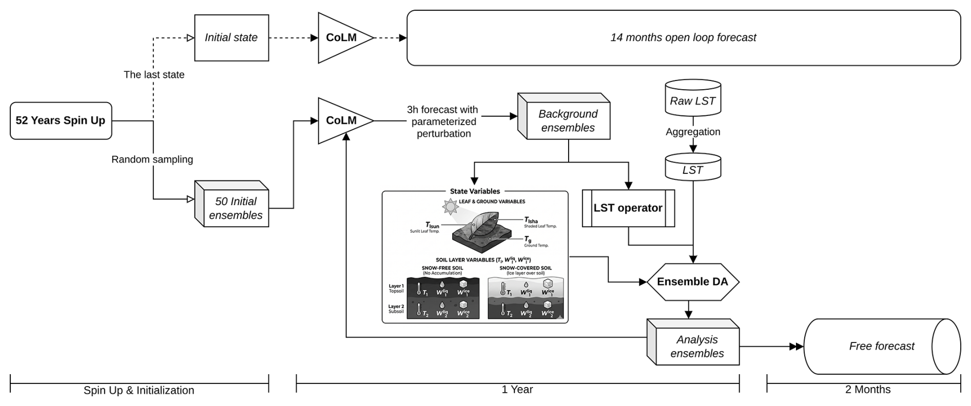
Figure 2 Schematic workflow of the coupling architecture and DA experiments. The process comprises a 52-year spin-up for initialization, a 1-year period comparing the assimilation group (solid lines, continuous 3 h cycles updating leaf, ground, and soil variables) against the open-loop baseline (dashed lines), and a subsequent 2-month free forecast.

After assimilation, to prevent model shock by restricting updates within the statistically reliable ensemble spread, if the magnitude of the analysis increment of a quantity x is three times larger than the standard deviation of its background, the analysis increment is clipped as follows:

$$\begin{array}{}\text{(19)}& \left\{\begin{array}{rl}{\displaystyle }\mathit{\sigma }& {\displaystyle }=\sqrt{{\displaystyle \frac{{\sum }_{k=\mathrm{1}}^K(x_k^{\text{b}}-{\stackrel{\mathrm{‾}}{x}}^{\text{b}}{)}^{\mathrm{2}}}{K-\mathrm{1}}}},\\ {\displaystyle }{x}_k^{\text{a}}& {\displaystyle }=min(x_k^{\text{b}}+\mathrm{3}\mathit{\sigma },max(x_k^{\text{b}}-\mathrm{3}\mathit{\sigma },x_k^{\text{a}}\left)\right).\end{array}\right.\end{array}$$

To ensure thermodynamic consistency, snow variables are only updated when all ensemble members reach a consensus on the presence of snow and possess an identical number of snow layers. In addition, if the analyzed liquid water (W^liq) and solid water (W^ice) amounts are negative, they are reset to zero. To maintain stable model integration, a small amount of ice is redistributed from the first soil layer to the second if solid ice is present in the top layer but absent in the second. Finally, the snow water equivalent is recalculated through the accumulation of the updated water mass within the snow layers for consistency.

3.3 Evaluation Metrics

The ensemble mean of the assimilation experiment is compared with the open-loop experiment and the evaluation datasets. The following metrics are used:

$$\begin{array}{}\text{(20)}& \left\{\begin{array}{l}\text{RMSD}=\sqrt{{\displaystyle \frac{{\sum }_{n=\mathrm{1}}^N({\widehat{y}}_n-y_n{)}^{\mathrm{2}}}{N}}},\\ R={\displaystyle \frac{{\sum }_{n=\mathrm{1}}^N{\widehat{y}}_n^{\prime }{y}_n^{\prime }}{\sqrt{{\sum }_{n=\mathrm{1}}^N{\widehat{y}}_n^{\prime \mathrm{2}}}\sqrt{{\sum }_{n=\mathrm{1}}^N{y}_n^{\prime \mathrm{2}}}}},\\ \text{BIAS}={\displaystyle \frac{{\sum }_{n=\mathrm{1}}^N({\widehat{y}}_n-y_n)}{N}},\\ \text{unbiased RMSD}=\sqrt{{\displaystyle \frac{{\sum }_{n=\mathrm{1}}^N({\widehat{y}}_n^{\prime }-y_n^{\prime }{)}^{\mathrm{2}}}{N}}},\end{array}\right.\end{array}$$

where ${\widehat{y}}_n^{\prime }={\widehat{y}}_n-\stackrel{\mathrm{‾}}{\widehat{y}}$, $y_n^{\prime }=y_n-\stackrel{\mathrm{‾}}{y}$, with $\stackrel{\mathrm{‾}}{\widehat{y}}=\frac{{\sum }_{n=\mathrm{1}}^N{\widehat{y}}_n}{N}$, $\stackrel{\mathrm{‾}}{y}=\frac{{\sum }_{n=\mathrm{1}}^N{y}_n}{N}$, and ${\widehat{y}}_n$ and y_n denoting the model outputs and validation datasets, respectively. We also compute the metric differences (AEXP -− OEXP) to highlight improvements.

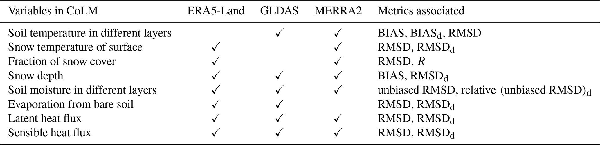
The details of the variables along with the metrics used for the evaluation against the gridded products are presented in Table 2. The metrics are selected based on the error characteristics of each variable. Specifically, soil moisture evaluation employs the unbiased RMSD to mitigate systematic biases arising from differing soil layer definitions across products, thereby focusing on the capture of dynamic variations. For other variables, absolute metrics such as RMSD and BIAS are used to evaluate their overall accuracy. The associated metrics include BIAS, root mean square difference (RMSD), unbiased RMSD (RMSD after removing the mean bias), and correlation coefficients (R). To directly demonstrate the effect of the assimilation compared to the open loop, the metric differences between the two experiments are defined as ${\text{BIAS}}_{\text{d}}=\left|{\text{BIAS}}_{\text{AEXP}}\right|-\left|{\text{BIAS}}_{\text{OEXP}}\right|$, ${\text{RMSD}}_{\text{d}}={\text{RMSD}}_{\text{AEXP}}-{\text{RMSD}}_{\text{OEXP}}$, $(\text{unbiased RMSD}{)}_{\text{d}}=(\text{unbiased RMSD}{)}_{\text{AEXP}}-(\text{unbiased RMSD}{)}_{\text{OEXP}}$, and $R_{\text{d}}=R_{\text{AEXP}}-R_{\text{OEXP}}$, where negative values of BIAS_d, RMSD_d, and (unbiased RMSD)_d indicate that the assimilation reduces the error relative to the open loop, while positive values of R_d indicate an improved correlation. With respect to the evaluation of soil moisture with the ERA5-Land and MERRA2, instead of the (unbiased RMSD)_d, the $\text{relative}(\text{unbiased RMSD}{)}_{\text{d}}=(\text{unbiased RMSD}{)}_{\text{d}}/\left(\right|\left(\text{unbiased RMSD}{)}_{\text{OEXP}}\right|)$ is used because the denominator can be very small. The selection of reference datasets in Table 2 is primarily dictated by data availability; for instance, GLDAS lacks snow surface temperature and snow cover fraction data, while MERRA2 does not provide bare soil evaporation. For the independent satellite and in-situ observations, the RMSD_d is specifically adopted to quantify the improvements in snow cover fraction and surface heat fluxes.

Table 2 Variables evaluated against the three gridded reanalysis/model products.

4 Results

4.1 Validation based on MODIS-LST

Figure 3a shows the RMSD_d of LST based on MODIS-LST for 31 January 2001–28 February 2002. It can be seen that, based on the previous 3 h analysis in AEXP, the predicted background LST is closer to the MODIS-LST compared with OEXP. This is evident from Fig. 3a since there are more negative (cyan) than positive (red) dots for RMSD_d. Specifically, the number (1995) of negative values for RMSD_d roughly doubles that (999) of the positive values. This is clearer from the daily mean (solid black line in Fig. 3a). As exhibited in the two-month free forecast (pink background in Fig. 3a), the accumulated effect within the one-year assimilation of MODIS-LST persists for at least 2 months.

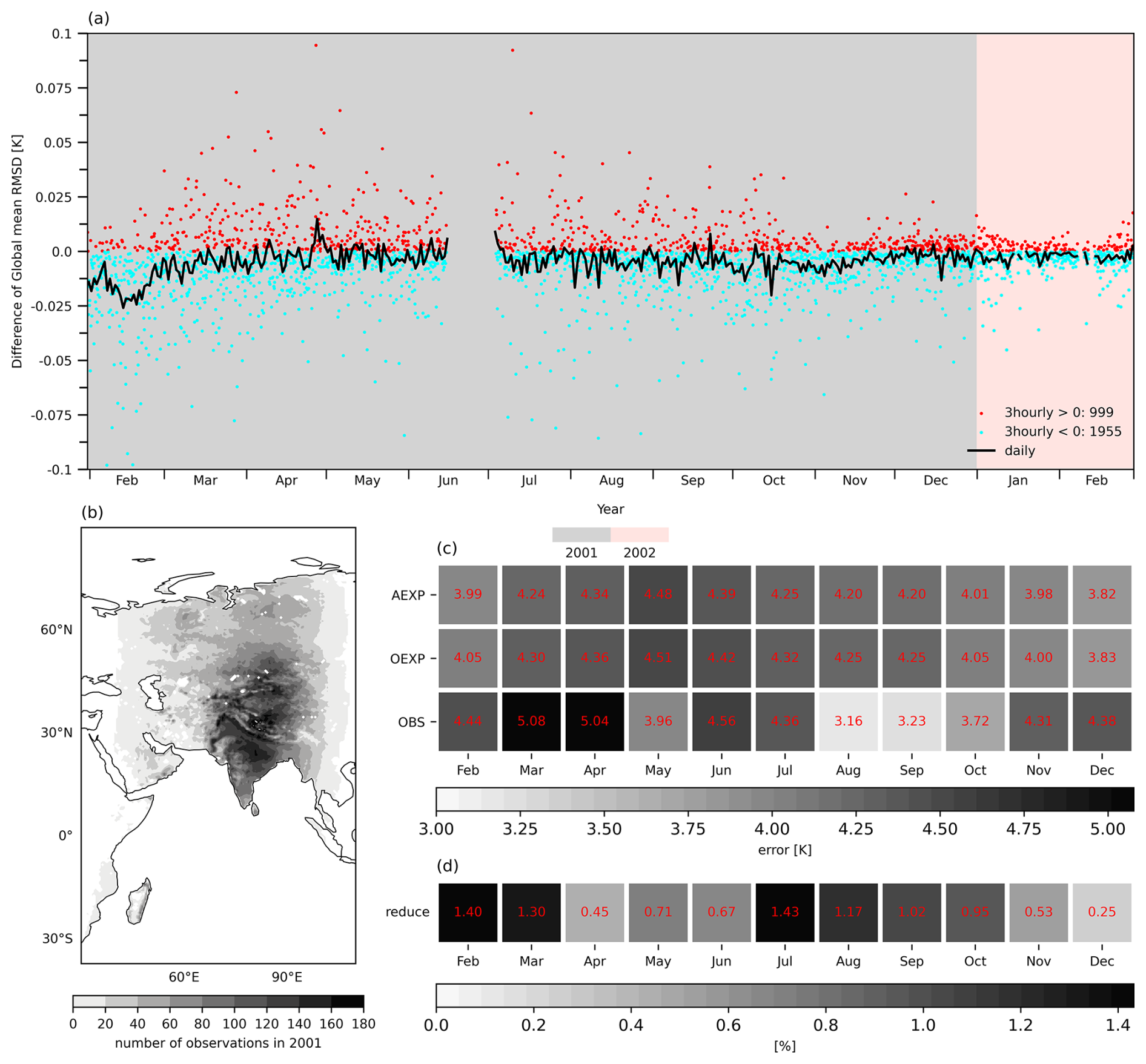
Figure 3 (a) Global LST RMSD_d based on the MODIS-LST from 31 January 2001 to 28 February 2002 in 3 h intervals (red and cyan dots for positive and negative values, respectively) and daily mean (solid black line), as the observations are not available in some days between June and July (blank areas). The number of positive and negative values is shown in the legend. Gray and pink backgrounds represent the period of cycle DA and free forecast, respectively. (b) Number of observations centered at 06:00 UTC within the time window from 1 January–31 December 2001. (c) Eastern Hemisphere monthly mean spatially averaged error for observations (third row) and the LST RMSD for AEXP (first row) and OEXP (second row) based on the MODIS-LST, and (d) relative reduction in percent of LST RMSD from OEXP to AEXP.

The small differences between the two experiments, as indicated by the absolute values of RMSD_d in Fig. 3a (with the maximum absolute difference of about 0.1 K), are consistent with the previous discussions on the nature of LST (Swinbank et al., 2003; Jin and Dickinson, 2010). LST is strongly influenced by land-atmosphere interactions, whereas in an offline model, this bidirectional interaction reduces to an unidirectional forcing from the atmosphere. Furthermore, the deterministic atmospheric forcing strictly constrains the background LST. Therefore, for LST, which largely depends on the interaction between the land and atmosphere, it is not surprising that the differences introduced by the assimilation are quickly damped by the same atmospheric forcing during the 3 h forecast lead time.

The example depicted in Fig. 3b illustrates the number of observations centered on 06:00 UTC in the Eastern Hemisphere counting from 1 January 2001 to 31 December 2001. The maximum number is centered at about 80° E. Figure 3c exhibits the error of observations, RMSD for both the AEXP and the OEXP in the Eastern Hemisphere. It is shown that the error of observations (i.e., observation uncertainty) has a considerable fluctuation in different months, with the largest error emerging in March (5.1 K) and the smallest one in August (3.2 K). Compared with the global scale (figures omitted), over Asia the AEXP shows pronounced improvement over the OEXP, with all months exhibiting reductions in RMSD (the largest reduction, 1.43 %, occurs in July), indicating region-dependent LETKF performance and the added value of observations.

4.2 Evaluation based on third-party datasets

4.2.1 Impacts on Soil and Snow Temperature

Comparisons between the two experiments on soil temperature in different layers based on GLDAS and MERRA2 datasets are presented in Figs. 4 and 5. The yearly BIAS_OEXP based on GLDAS is illustrated in the first column of Fig. 4. It can be inferred that the CoLM exhibits a large positive BIAS in depicting soil temperature in several regions, including western North America, western South America, South Africa, the Tibetan Plateau and Northeast Asia. These regions typically are arid zones, plateau areas, or permafrost soils. In contrast, relatively small negative BIAS is observed in Alaska, the southern part of the Middle East, and some areas of Northeast Asia.

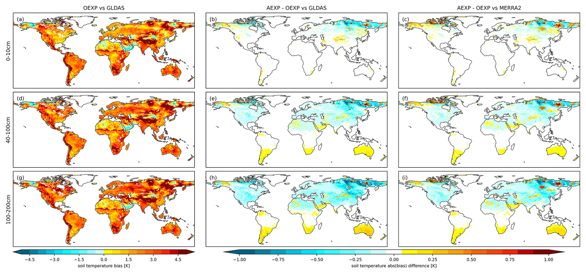
Figure 4 Soil temperature (in K) yearly (31 January 2001 to 31 December 2001) BIAS based on GLDAS of OEXP (first column) and BIAS_d based on GLDAS (second column) and MERRA2 (third column): (a–c) for 0–10 cm, (d–f) for 40–100 cm, and (g–i) for 100–200 cm.

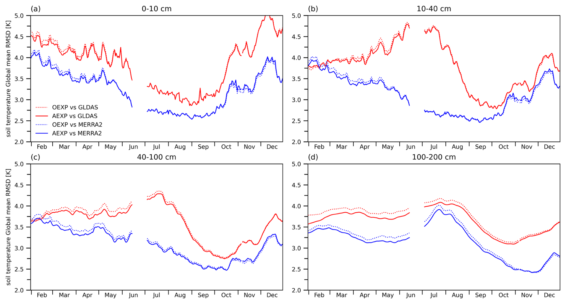
Figure 5 Soil temperature (in K) global RMSD of OEXP (dotted line) and AEXP (solid line) based on GLDAS (red) and MERRA2 (blue): (a) for 0–10 cm, (b) for 10–40 cm, (c) for 40–100 cm, and (d) for 100–200 cm.

The second and third rows in Fig. 4 mostly demonstrate the considerable improvements of the assimilation over the open loop based on the third-party datasets. In terms of the yearly BIAS_d based on the GLDAS dataset (Fig. 4b, e and h), the maximum improvements in BIAS are centered on Northeast Asia (BIAS is reduced by approximately 1.0, 1.5, and 2.0 K for depths 0–10, 40–100, and 100–200 cm, respectively). This pattern of improvement is also distributed across most parts of eastern Asia, Europe, and eastern North America, which are mostly humid areas. Although improvements are evident in the Northern Hemisphere, small degradations emerge in the Southern Hemisphere, with the maximum centered on southern South America, South Africa, and Australia, which are typical arid zones in the LSM. These results suggest that the assimilation scheme effectively updates soil temperature in relatively humid areas and reduces bias appropriately. However, the effect of bias reduction is not pronounced in arid zones. A similar pattern can be seen in Fig. 4c, f, and i, which are based on the MERRA2 datasets.

Improvements are also evident from Fig. 5, where the RMSD_AEXP is smaller than RMSD_OEXP throughout the assimilation period with both GLDAS and MERRA2 benchmark datasets. The reduction of RMSD approximates 0.1 and 0.2 K for depths 0–10 and 100–200 cm, respectively, in particular, on 31 January 2001 with the GLDAS benchmark dataset. It can also be inferred from the temporal variation of RMSD of both experiments that the influence on soil temperature is depth dependent, as can be seen from Fig. 5, as the depth increases, taking MERRA2 as an example, the minimum RMSD occurs in August, September, October and November, indicating different memory effects in different soil layers.

Apart from both temporal and spatial improvements, the most promising finding is the dependence of improvements on the depth of soil layers. While relatively small improvements are observed in the upper soil layers (Figs. 4b and c, 5a), the improvements tend to become more significant in the deeper soil layers (Figs. 4e, f, h, and i, 5b–d), which is consistent with the nature of the land process. Although the soil temperature within the upper layers can be easily modulated by changes in the land-atmosphere interaction, energy stored in the deeper soil layers, especially within 100–200 cm, cannot be directly influenced by this interaction. Consequently, the signals modified by assimilating LST into CoLM can be transferred to and persist longer in these deeper soil layers, maintaining their influence within them for a longer time. Furthermore, the modified signals within the deep layers are not directly updated by assimilating MODIS-LST, but through the vertical exchange of water and energy with the upper layers. In other words, although the energy stored in the upper soil layers cannot persist in the upper layers, its influence can be transferred into the deeper layers through vertical diffusion between different soil layers. After MODIS-LST is assimilated into CoLM to update the upper soil temperature and water content, the changed signals within the upper layer are transferred to deeper layers, as the latter can store this signal for a relatively longer time. This result suggests promising potential for the assimilation scheme presented in this study, which utilizes MODIS-LST to jointly update soil temperature and moisture in the upper soil layer, after which the modified signals are transferred into deeper soil layers through the vertical diffusion by CoLM during the forecast phase.

The temperature of snow is vital for estimating both the energy and the water balance of the land surface layer. Figure 6 reveals the effectiveness of using MODIS-LST to update both snow temperature and water content consistently. It can be observed from Fig. 6a that CoLM exhibits relatively large RMSD of snow temperature based on ERA5-Land, centered in Northeast Asia and the northern regions of North America. Similar patterns are evident in Fig. 6d, g, and j for different seasons, with maximum uncertainties centered in the same areas as in Fig. 6a (results based on MERRA2 datasets are similar and not shown here). The largest RMSD values occur in February, indicating the challenges faced by CoLM in accurately representing snow temperature, particularly during winter for high-latitude regions (December also exhibits large RMSD values, not shown here). While snow temperature strongly depends on the water content, we attribute this unsatisfactory depiction of snow temperature to the deficient snow processes in LSM.

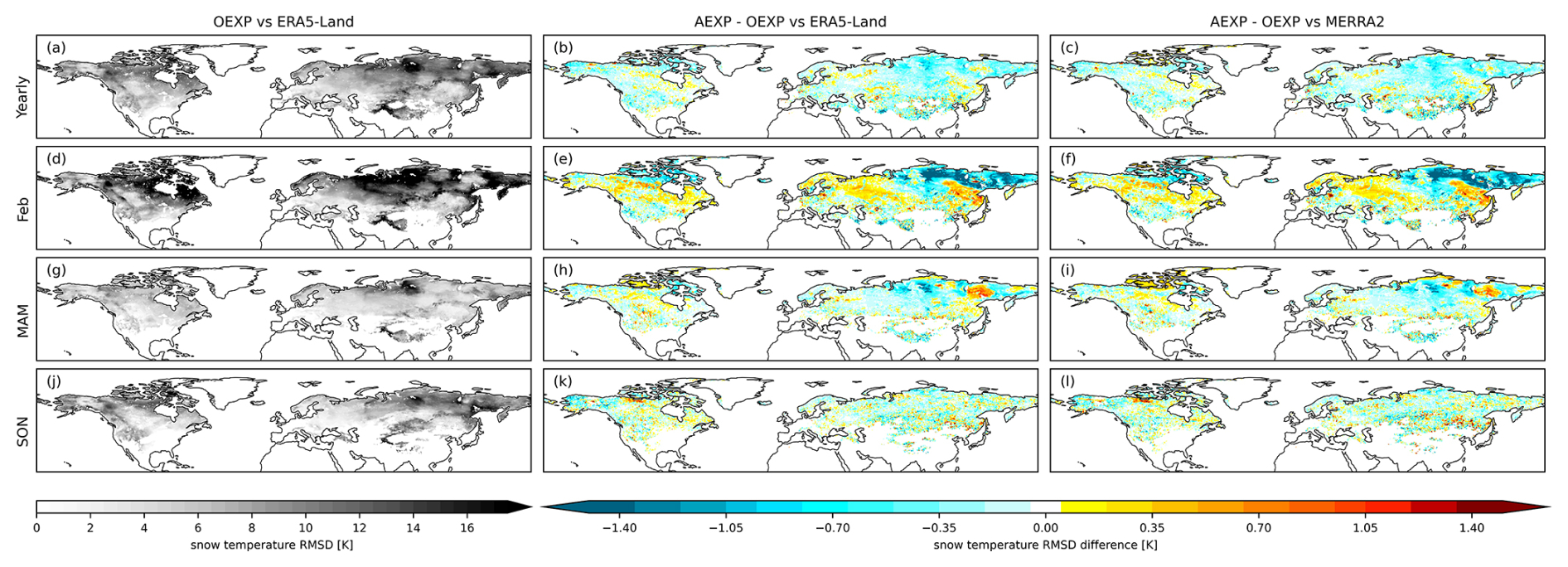
Figure 6 Snow temperature (in K) RMSD based on ERA5-Land (first column) of OEXP and RMSD_d based on ERA5-Land (second column) and MERRA2 (third column) for (a–c) yearly, (d–f) February, (g–i) MAM (March–April–May), and (j–l) SON (September–October–November).

Compared with the open loop, improvements in snow temperature by assimilation are evident in Fig. 6b and c. Most regions exhibit improvements, with the maximum enhancements centered in Northeast Asia, similar to the patterns observed for soil temperature shown in Fig. 4b and c. This similarity suggests that snow water content effectively modulates the updated snow temperature, particularly during winter (Fig. 6e and f), with maximum RMSD_d values larger than 4 K in Northeast Asia for both ERA5-Land and MERRA2 datasets. This indicates that when the snow mass largely covers the soil layers, it insulates the soil beneath.

4.2.2 Improvements in Snow Properties and Soil Moisture Content

Unlike previous studies that used LST to update either soil temperature or soil water content, the assimilation scheme proposed in this study employs MODIS-LST to jointly update both soil temperature and water content in the upper layers through the framework of EnKF. Under this assimilation scheme, it is theoretically capable of producing consistent energy and water fields. Furthermore, one potential drawback of soil moisture assimilation is that the analysis increments only apply to soil moisture mass but cannot change its phase which depends on temperature. However, the joint update for both temperature and water content enables the water stored in snow or soil to change its phase between liquid and solid, especially in middle to high latitudes where the surface temperature is around the freezing/melting point. By simultaneously adjusting both state variables, this analysis allows water to redistribute between phases, yielding more realistic frozen/soil water partitions during the forecast phase.

The fraction of snow cover is a key parameter for indicating the temporal and spatial variation of snow water content. In high latitudes the fraction of snow cover may remain unchanged throughout the year due to the relatively low temperature below the melting point; the temporal variations of snow cover are considerably large in middle to high latitudes where the surface temperature range easily accommodates the condition for snow freezing or melting. In this study, we compare the snow cover from both experiments based on the ERA5-Land and MERRA2 datasets in terms of two global-scale metrics, and present the results in Fig. 7.

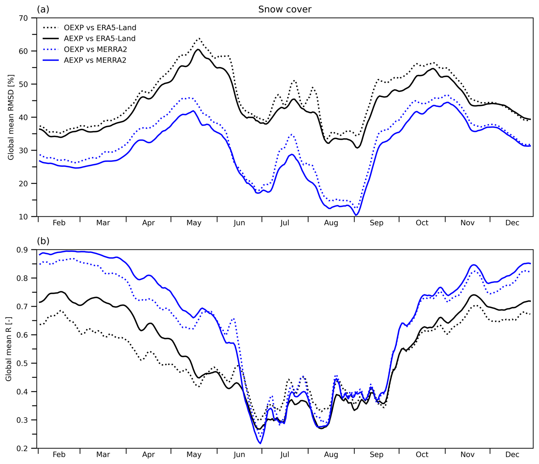
Figure 7 Snow cover (in %) global RMSD (a) and R (b) of OEXP (dotted) and AEXP (solid) based on ERA5-Land (black) and MERRA2 (blue).

It can be inferred from Fig. 7a that the simulation of snow cover in CoLM has relatively large uncertainties in early summer and early winter (RMSD reaches 60 % and 40 % in May, based on ERA5-Land and MERRA2, respectively), revealing a poor simulation of snow melting and freezing. Relatively small uncertainties emerge in winter and summer months when the temporal variations of snow cover are relatively small. In Fig. 7b, both experiments reach their minimum R in summer when the snow merely remains in high-altitude and high-latitude regions. Comparison between two experiments demonstrates that the most significant enhancement is in spring and autumn regardless of the benchmark datasets (ERA5-Land and MERRA2). This improvement underscores the promising potential of assimilating MODIS-LST to adjust the snow cover in CoLM, particularly during periods of snow melting and freezing.

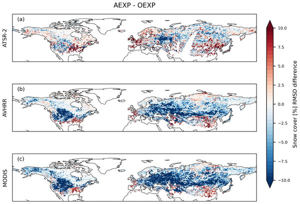
To further substantiate these findings with independent observations, the horizontal distribution of the yearly snow cover (in %) RMSD_d evaluated against three satellite datasets is presented in Fig. 8. As depicted, the assimilation of LST yields widespread improvements across the Northern Hemisphere, particularly over the mid-to-high latitudes of North America and Eurasia when evaluated against AVHRR (Fig. 8b) and MODIS (Fig. 8c), where most of these areas exhibit an RMSD reduction of approximately 10 %. While the evaluation against ATSR-2 (Fig. 8a) shows some regional degradations, the overall spatial patterns based on these three datasets robustly demonstrate the capability of the joint assimilation scheme to effectively constrain the surface thermal dynamics, thereby yielding a more physically consistent representation of snow accumulation and melting in the mid-to-high latitudes.

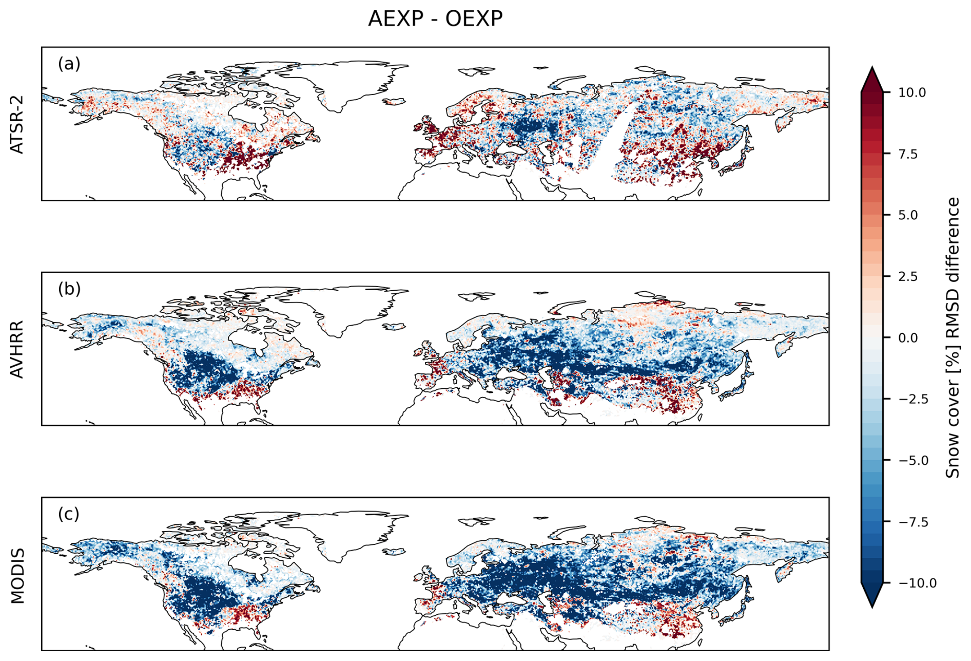
Figure 8 Snow cover (in %) yearly (31 January to 31 December 2001) RMSD_d evaluated based on different satellite products: (a) ATSR-2, (b) AVHRR, and (c) MODIS.

While snow cover is a key parameter indicating the fraction of snow within a grid cell, with strong temporal variations in middle-high latitudes and minimal disturbance in high latitudes, snow depth describes the cumulative effect of snow content within a grid cell. Changes in temperature, mass, and phase of water content all directly influence the simulation of snow depth from middle to high latitudes, making it a comprehensive parameter for estimating energy and water budgets related to snow content. Even excluding the permanent snow regions of Greenland and Antarctica, snow depth still exhibits significant spatial variation across different continents. In this study, the spatial BIAS of snow depth based on the three datasets is provided in Fig. 9.

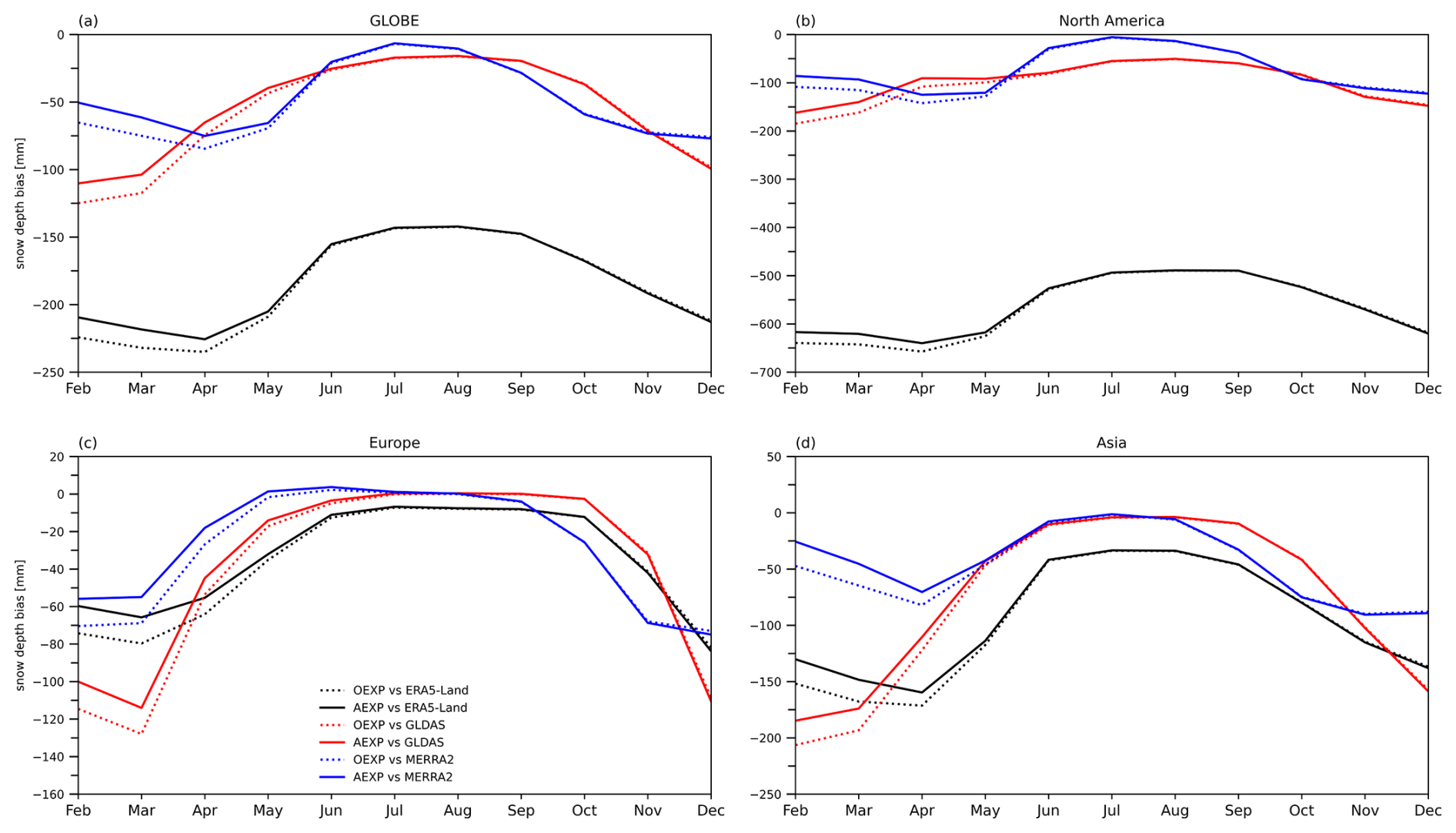
Figure 9 Snow depth (in mm) BIAS of OEXP (dotted) and AEXP (solid) based on ERA5-Land (black), GLDAS (red) and MERRA2 (blue). (a) For global excluding Antarctica, (b) for North America, (c) for Europe, and (d) for Asia.

It can be seen from Fig. 9 that the BIAS for snow depth reaches a minimum in summer, as snow mass is relatively low when the Northern Hemisphere receives much solar radiation. The BIAS based on GLDAS and MERRA2 is consistent over either the globe (Fig. 9a) or different continents (Fig. 9b–d). In contrast, BIAS based on ERA5-Land exhibits a large discrepancy from those based on GLDAS and MERRA2 over the globe (Fig. 9a) and North America (Fig. 9b). This indicates that, over North America, the snow depth simulated by the LSM used in the ERA5-Land is vastly different from that by the CoLM and the LSMs used in the GLDAS and MERRA2. Regardless of the benchmark datasets, the large negative BIAS in simulating snow water content by the CoLM occurs in late winter and early spring, and so does the large improvement by assimilation for snow depth.

Taking into account the seasonal variations in snow depth, RMSD_d is shown in Fig. 10 (summer time is not shown here due to the relatively small magnitude). In general, improvements are observed for most regions in the Northern Hemisphere throughout the year and different seasons, with the largest enhancements (up to 150 mm in February) centered in Northwest Asia. Consistent with snow temperature, the assimilation yields the largest RMSD reductions in winter (RMSD based on GLDAS reduces over 100 mm in northwest Asia as shown in Fig. 10e), with relatively small improvements in other seasons.

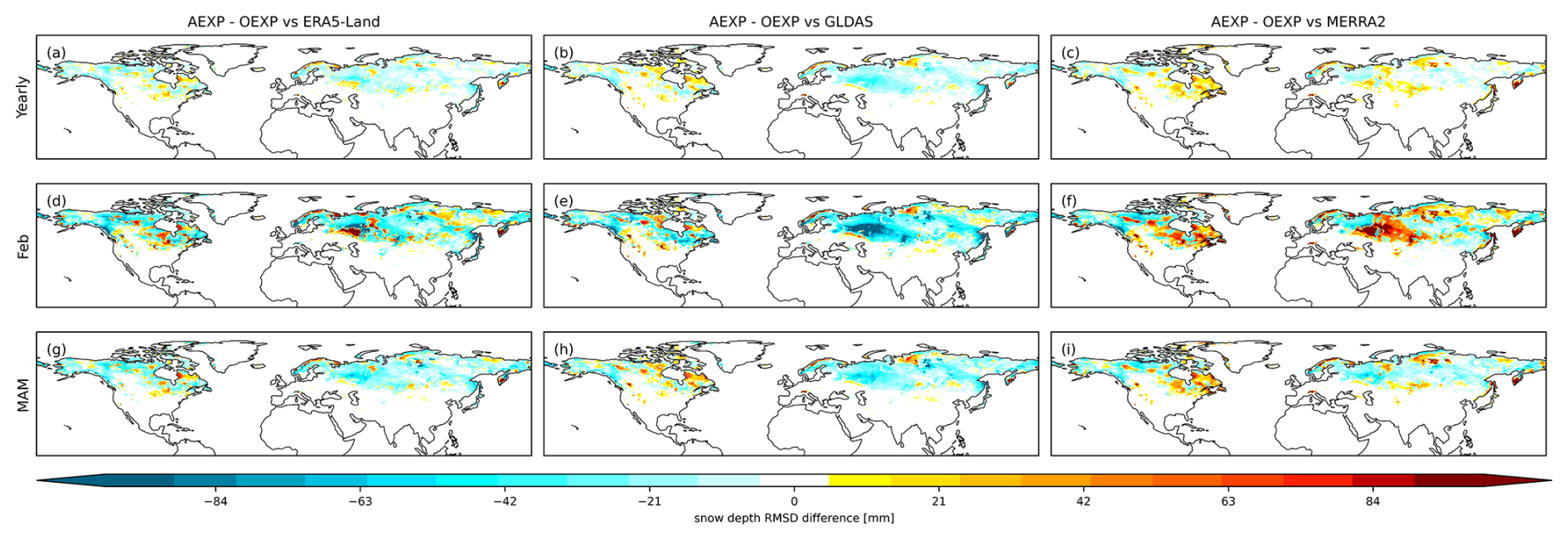
Figure 10 Snow depth (in mm) RMSD_d based on ERA5-Land (first column), GLDAS (second column), and MERRA2 (third column). (a–c) For year, (d–f) for February and (g–i) for MAM (March–April–May).

After discussing the results of the water content above the soil layers, the remainder of this section focuses on the water content (solid plus liquid phase) within the soil layers, as shown in Figs. 11 and 12. It can be observed from Fig. 11a and c that large uncertainties emerge in the Northeast regions of North America and Northern Eurasia, as most of these regions are considered humid areas with high soil moisture. The minimum uncertainties are observed in Northern Africa, the Middle East, and the Junggar Basin, as most of these regions are regarded as arid areas with low soil moisture. These results show that CoLM has a relatively adequate simulation of soil moisture in regions with low humidity but an insufficient simulation of soil moisture in regions with high humidity.

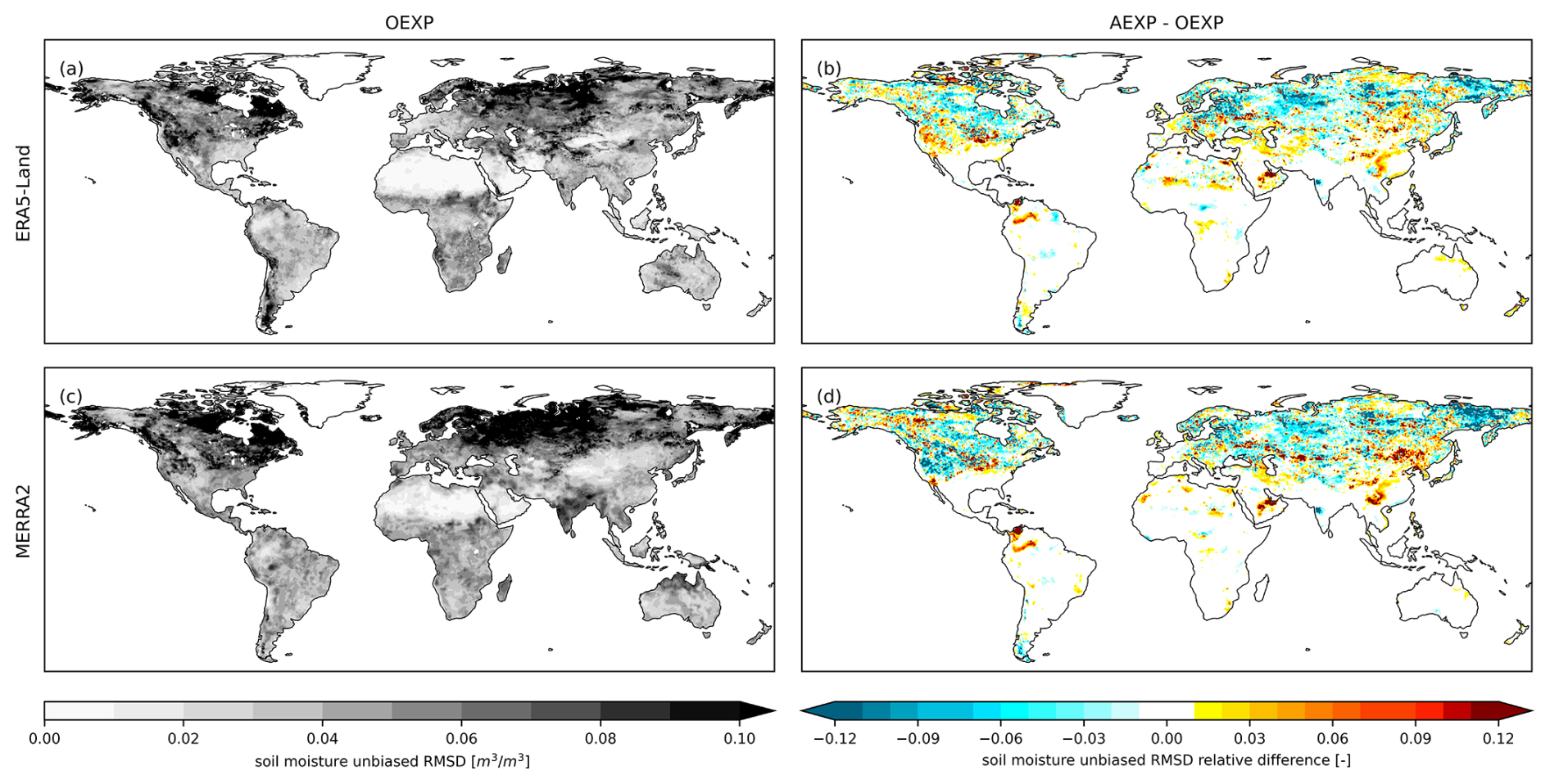
Figure 11 Soil moisture (in m³ m⁻³) yearly (31 January to 31 December 2001) unbiased RMSD of OEXP (first column) and relative (unbiased RMSD)_d (second column) in the upper soil layer based on (a, b) ERA5-Land and (c, d) MERRA2.

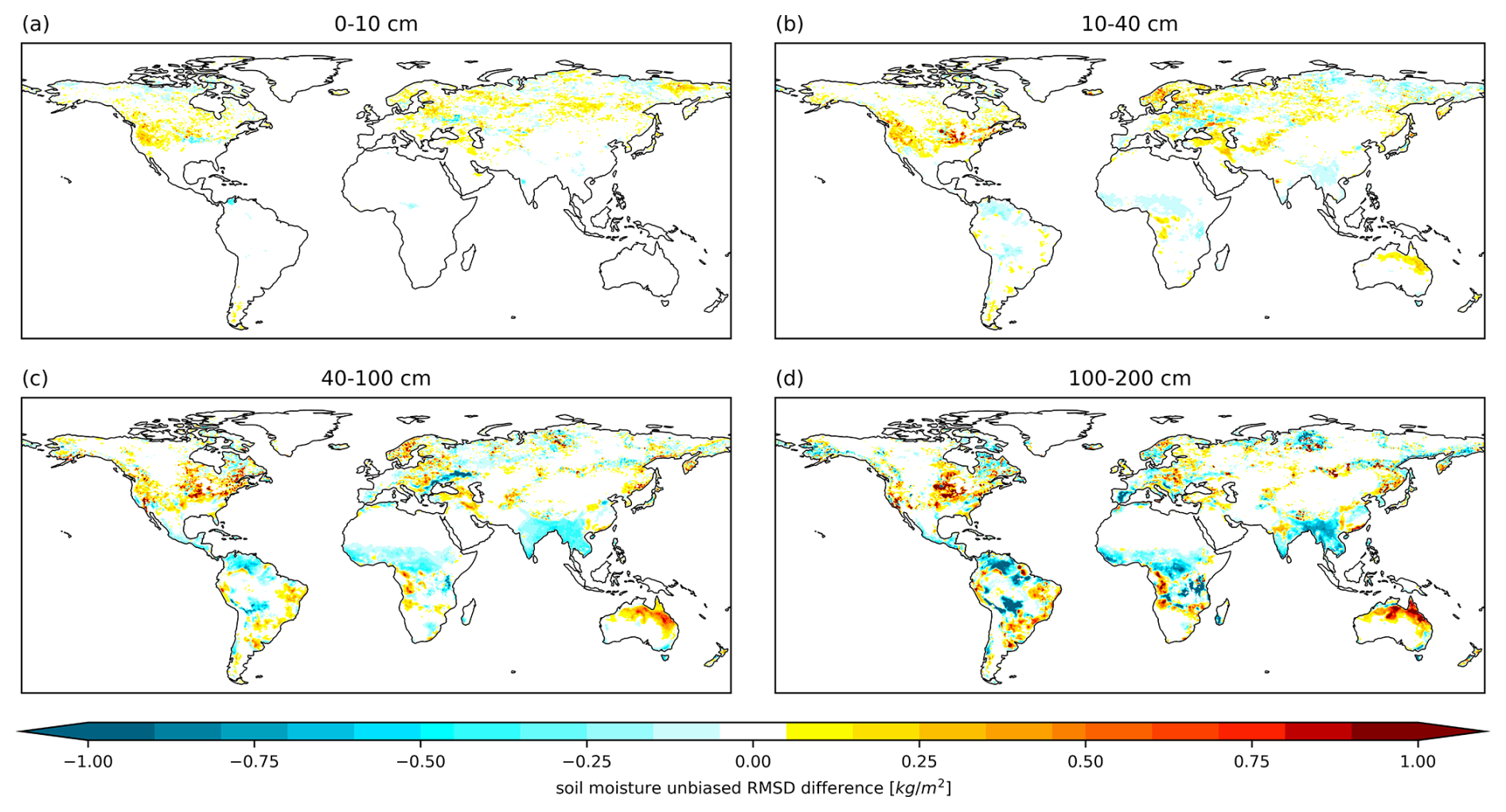
Figure 12 Soil moisture (kg m⁻²) yearly (from 31 January to 31 December 2001) (unbiased RMSD)_d based on GLDAS: (a) for 0–10 cm, (b) for 10–40 cm, (c) for 40–100 cm and (d) for 100–200 cm.

Improvements in unbiased RMSD occur in regions with relatively large uncertainty in the soil moisture simulation. Three maximum enhancements are observed in North America, Northern Eurasia, and Northeast Asia, as shown in Fig. 11b and d. The largest improvements, centered on northern Asia based on MERRA2 datasets, reach a 40 % reduction. It is also noteworthy that significant improvements in soil moisture within the upper soil layer emerge in high latitudes in the Northern Hemisphere, suggesting the effectiveness of the assimilation scheme, which jointly updates temperature and water content to obtain more realistic and consistent updated model fields for energy and water content. In other words, while the updated soil water content has a direct influence on the mass of water, the temperature change in the upper soil layers also drives the water content to change its phase. This joint modification of soil moisture is most pronounced at mid- to high latitudes.

A comparison of the two experiments in different soil layers based on the GLDAS datasets is shown in Fig. 12. As the depth increases, the absolute value of the (unbiased RMSD)_d increases and reaches its maximum in the deepest soil layer within 100–200 cm, as shown in Fig. 12d. The maximum improvements are observed in northern regions of South America, central Africa, southern Asia, and northern Asia, where most regions are humid. Conversely, large degradations can be found in central areas of North America, eastern South America, and northern Australia, where most regions are relatively dry. Furthermore, localized degradations in Fig. 12 also occur in western North America and parts of northern Asia, where strong nonlinearity during seasonal freeze–thaw transitions makes the exact timing of phase changes difficult to capture. Additionally, performance degradation around open waters, such as the Great Lakes, is likely caused by the artificial alteration of land–lake thermal gradients. Updating only land grids while excluding water bodies disrupts localized secondary circulations, thereby weakening the assimilation benefits in these specific boundary regions.

Increasing improvements are seen as the soil depth increases, which reveals that the soil moisture modified by the assimilation within the upper layers is transferred down to the deep layers through vertical exchange among soil layers (taking the Amazon Rainforest as an example, the largest reduction in unbiased RMSD is about 0.06, 0.12, 0.15, and 6.58 kg m⁻² based on GLDAS datasets for soil layers of 0–10, 10–40, 40–100, and 100–200 cm, respectively). This conclusion aligns with those summarized from the soil temperature comparisons shown in Fig. 4. Unlike the surface layer, which has a strong connection with the above atmospheric conditions, the water stored in the deep layers can be regarded as a contribution from both the internal variation of soil water content within the layer and the accumulative effect of transferred modified signals from upper layers.

Furthermore, we attribute improvements in South America, central Africa, and southern Asia within the deepest soil layer to the high water conductivity in these humid areas, allowing for fast and efficient vertical transfer from the top soil layer to the bottom. In contrast, in central areas of North America, eastern South America, and northern Australia, it is challenging to transfer the modified information within the upper layers to the deep layers through vertical exchange owing to the relatively low water conductivity.

4.2.3 Modulations of Evaporation and Surface Heat Fluxes

Although evaporation and heat flux do not directly feedback on the prediction of land surface variables in offline LSMs, they provide key insights for studies in coupled models. Comparing these crucial fluxes against established datasets allows us to assess the model's performance and sheds light on the effectiveness of assimilation in improving the representation of land-atmosphere interactions.

Large RMSD values are observed in eastern North America, northern South America, central Africa, and central Asia for all three variables (Fig. 13). These regions are known for their high humidity, indicating relatively large uncertainties in the flux simulated by CoLM in humid regions. Conversely, there is relatively high confidence in areas with low humidity, such as northern Africa and the Middle East, as depicted in Fig. 13a, d, and h.

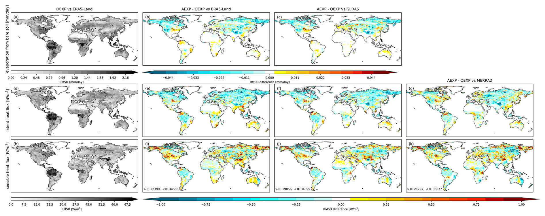
Figure 13 Yearly (from 31 January to 31 December 2001) RMSD based on ERA5-Land of OEXP (first column) and RMSD_d based on ERA5-Land (second column), GLDAS (third column) and MERRA2 (fourth column) for evaporation from bare soil (mm d⁻¹, first row), latent heat flux (W m⁻², second row), and sensible heat flux (W m⁻², third row). MERRA2 does not provide evaporation from bare soil, so no corresponding panel is shown in the first row. The number of the positive and negative values of RMSD_d for sensible heat flux is shown in (i), (j), and (k).

The Mediterranean region also exhibits a larger RMSD for evaporation from bare soil (Fig. 13a) compared with latent (Fig. 13d) and sensible (Fig. 13h) heat fluxes, which show no similarity of large RMSD. The RMSD in the Amazon Rainforest for evaporation (Fig. 13a) is not as significant as that for the latent heat flux (Fig. 13d). This difference between evaporation and latent heat flux can be attributed to the fact that evaporation from bare soil does not include transpiration from vegetation. There is abundant vegetation in the Mediterranean region and the Amazon Rainforest, where abundant vegetation enhances transpiration, thereby increasing latent heat flux while leaving bare-soil evaporation unchanged.

Obvious improvements can be found for the evaporative heat flux over western North America, the Tibetan Plateau, and Northeast Asia, as can be seen in Fig. 13b and c. The consistent pattern of RMSD_d in soil moisture (Fig. 11b) and in evaporation (Fig. 13b) based on the ERA5-Land dataset can be attributed to the fact that the changes in soil moisture within the upper soil layers have a direct influence on the amount of evaporation. This consistency is also found in the comparison between Fig. 12a and Fig. 13c based on GLDAS datasets.

The large improvements in Fig. 13b and c for evaporation flux from the bare soil, are also observed over similar regions in Fig. 13e–g for latent heat flux regardless of the benchmark datasets. Additionally, considerable improvements in the Amazon Rainforest are consistent with the findings aforementioned, and highlight the importance of considering transpiration from vegetation.

Large degradations are observed in Alaska, western regions of North America, the Tibetan Plateau, and Northeast Asia, while considerable improvements are shown in the Amazon Rainforest, central Africa, and eastern Asia for sensible heat flux. The partition of the available energy between latent and sensible heat fluxes depends strongly on the soil moisture. Taking Fig. 13e and i based on the ERA5-Land dataset as an example, improvements are observed for both fluxes in regions with high humidity, such as the Amazon Rainforest and central Africa. In contrast, opposite patterns are observed in regions with relatively low humidity, such as western North America and Northeast Asia. This highlights that assimilation-induced changes in soil moisture can simultaneously modulate both fluxes, depending on the prevailing surface energy partitioning.

To further validate the assimilation impact on surface energy partitioning against independent ground truth, in-situ observations of sensible and latent heat fluxes from the FLUXNET2015 and AmeriFlux networks are incorporated. The corresponding site-specific evaluation is presented in Fig. 14. As illustrated in the spatial distribution (Fig. 14a), the assimilation scheme yields clear improvements at the majority of the evaluated sites globally. Most locations exhibit enhanced performance in both heat fluxes (green circles) or at least one flux variable (orange triangles). Quantitatively, the site-specific RMSD_d (Fig. 14b) reveals consistent and often substantial error reductions for the latent heat flux across most stations. In contrast, the response of the sensible heat flux exhibits greater site-to-site variability, which aligns with the mixed regional patterns observed in the gridded comparisons.

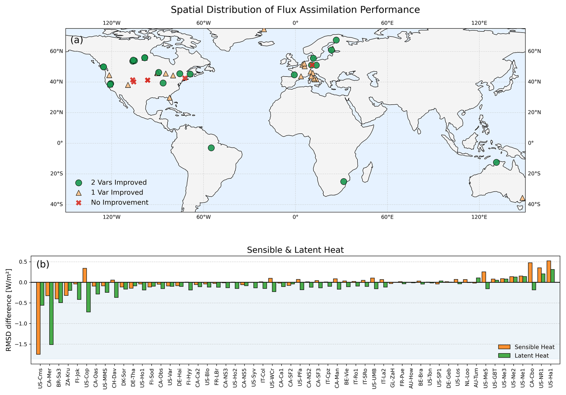
Figure 14 Spatial and quantitative evaluation of the impact of assimilation on surface heat fluxes across global sites. (a) Distribution of assimilation performance based on sensible heat and latent heat. Markers categorize sites by the number of improved flux variables: green circles indicate improvement in both heat fluxes, orange triangles represent improvement in a single variable, and red crosses denote no improvement. (b) Site-specific RMSD_d for sensible heat (orange bars) and latent heat (green bars) across the year (31 January to 31 December 2001).

5 Discussion

The most notable soil temperature difference between the assimilation and the open loop occurs in permafrost regions of Northeast Asia (Fig. 4b). Within this region the three reanalyses also differ markedly. GLDAS agrees well with MERRA2, whereas ERA5-Land yields substantially different soil temperature magnitudes. The BIAS_d based on ERA5-Land is positive globally (figures similar to Fig. 4b, e, h, c, f, and i are omitted). These positive values suggest degradation in soil temperature estimation worldwide. Given that the soil temperature from the ERA5-Land dataset is known to carry a relatively large bias in permafrost regions (Cao et al., 2020), we exclude it from the evaluation process, as indicated in Table 2.

Wide discrepancies among the third-party datasets remain, most notably for snow depth, as shown in Fig. 9a. While the BIAS global mean based on GLDAS and MERRA2 is around −75 mm, that based on ERA5-Land datasets is approximately −200 mm. While the RMSD_d based on ERA5-Land is nearly identical to that based on GLDAS (Fig. 10d and e), it is opposite to that based on MERRA2, which indicates degradation in central Eurasia and eastern regions of North America (Fig. 10f).

Despite the notable differences observed for certain variables among different third-party datasets, it is reassuring to observe relatively consistent results across different datasets for most variables on a global scale. This consistency underscores the importance of utilizing diverse datasets in the evaluation process. By incorporating multiple datasets, the evaluation results become more robust, providing a confident understanding of the performance of both the CoLM and DA method and reducing the impact of biases or uncertainties inherent in any single dataset. Furthermore, the performance enhancements yielded by this study are generally comparable to relevant previous studies. Huang et al. (2008) assimilated LST to update soil temperature, reporting an error reduction of approximately 1 K at specific sites. This aligns with our results, which show a bias reduction of 1.0–2.0 K with increasing depth over Northeast Asia (Fig. 4). Furthermore, while Chen et al. (2021) assimilated both LST and brightness temperature to achieve a 19 %–71 % RMSD reduction for shallow soil moisture on the Tibetan Plateau, the LST-only assimilation in this study yields a comparable impact, reducing the unbiased RMSD for upper-layer soil moisture by up to 40 % in Northern Asia (Fig. 11).

While the assimilation scheme proposed in this study does not take the bias correction (Bosilovich et al., 2007; Reichle et al., 2010) into account, it is noteworthy that one of the biggest challenges faced in this study is not the bias in either model forecasts or observations. Since the land surface processes are strongly influenced by the overlying atmosphere, the forecasts of an offline LSM are almost determined by the atmospheric forcing rather than the initial conditions. Several studies have shown unrealistically small ensemble spread in the land surface variables (Muñoz-Sabater et al., 2021), such as the soil moisture content (Draper, 2021), in an offline LSM. Despite this inherent limitation, diagnostics of spread indicate that the ensemble members dynamically evolve without collapsing. Taking the Northern Hemisphere as an example, the temperature spread in the first soil layer is relatively low, ranging from 0.3 to 1.4 K, owing to the strong atmospheric forcing. This expected limitation further justifies the joint update of soil temperature and soil moisture. Meanwhile, the soil moisture spread increases from approximately 0.5 kg m⁻² at the surface to 10.0 kg m⁻² in the deepest layer, accompanied by physically consistent seasonal variations.

Direct inflation of the analysis covariance is not used in this study. In the forecast phase, the CoLM perturbs its tunable parameters to generate ensemble forecasts as the background for next cycle, with the purpose of not only accounting for the model error but also inflating the covariance. Physically, this tuning strategy modulates six core land surface processes: surface turbulent exchange, canopy and snow hydrology, runoff generation, alongside soil thermal and water dynamics. Perturbing these specific mechanisms is essential for LST assimilation, as the simulated LST is predominantly sensitive to parameters governing the surface energy balance and outgoing radiation. Furthermore, parameters regulating energy storage and water retention directly dictate the hydro-thermal cross-covariance, which ensures a physically consistent joint update of temperature and moisture. The parameters are perturbed up to 15 % of the corresponding parameter's absolute value (see Sect. 2.1), which is neither too small for the aforementioned reason nor too large for model stability. Although the improvements during the free prediction time (Fig. 3a), it is noticeable that the difference between the assimilation and the open loop tends to decrease as time increases, as shown in Figs. 5b–d and 9.

6 Conclusions

In this study, the LETKF is applied to the CoLM for the first time. MODIS-LST from the Terra satellite is assimilated throughout 2001, followed by a 2-month free forecast. Unlike previous studies that used LST to update either the temperature or the water content within the soil layers, the assimilation scheme proposed in this study jointly updates both soil temperature and water content in the upper layers to prolong the influence of the LST assimilation. On the one hand, the jointly updated temperature and water content by assimilating MODIS-LST have a relatively larger capacity for storing and retaining the influence from LST. On the other hand, it is theoretically more likely to produce both energy and water fields in a consistent manner, especially for middle to high latitudes where the surface temperature is around the freezing or melting point, which enables the updated temperature within the soil and snow layer to change the phase of water content. Additional experiments demonstrate that this joint update outperforms updating only soil temperature, improving both the soil water and energy states (Fig. 1) and also snow-related variables (results not shown here). The evaluation based on the MODIS-LST shows a relatively small enhancement, consistent with the nature of LST which is strongly determined by the atmospheric forcing in an offline LSM. Considerable improvements are seen for other variables based on three benchmark datasets, such as the soil temperature, with the largest BIAS reduction centered in Northeast Asia and its magnitude increasing as the depth increases (about 1.0, 1.5, and 2.0 K for 0–10, 40–100, and 100–200 cm, respectively), indicating the signals induced by assimilating LST can be transferred to and persist longer in deeper soil layers. Similar to soil temperature, the maximum improvements in snow temperature and snow depth also occur over Northeast Asia, with a reduction of RMSD of about 4 K and 150 mm, respectively. This improvement over middle to high latitudes indicates the effectiveness of the joint update on the temperature and water content, which is allowed to change its phase depending on the changed temperature. Furthermore, improvements in soil water content are seen, especially in the humid regions within the tropics; taking the Amazon Rainforest as an example, the largest reduction in unbiased RMSD is about 0.06, 0.12, 0.15, and 6.58 kg m⁻² for depths of 0–10, 10–40, 40–100, and 100–200 cm, respectively, indicating the high water conductivity in these humid areas, which allows for fast and efficient vertical transfer from the top soil layer to the bottom.

The challenge of maintaining a realistic ensemble spread for ensemble assimilation into offline LSMs remains open. Thus, it might be more effective for ensemble-based land surface DA to use a coupled model with two-way coupling between the land and atmosphere. Assimilating satellite radiance observations in the atmospheric window into a land-atmosphere two-way coupling model has been undergoing investigation and will be presented in another paper.