Simulating SAR altimeter echoes from cryospheric surfaces with the Snow Microwave Radiative Transfer (SMRT) model version 1.7

Radar altimeters are essential tools for observing the cryosphere, especially for estimating ice-sheet elevation change and sea-ice thickness. However, retrieving these quantities remains challenging, and progress depends on physically based numerical simulations of the recorded waveforms to understand their sensitivity to the geophysical parameters of the medium. Such models can also guide the design of future satellite missions. Accurate simulations require a balanced combination of a realistic description of the medium, precise calculation of wave–medium interactions, and an accurate representation of the altimeter measurement process, including downstream processing. The Snow Microwave Radiative Transfer (SMRT) model has addressed the first two aspects for a decade and includes an altimetric Low Resolution Mode (LRM) module, but has, until now, lacked a delay-Doppler (SAR) altimetric capability used by most modern sensors. This study introduces the new SMRT SAR altimetry module, which operates in three steps. First, it calculates the backscatter of all layers and interfaces using existing SMRT modules. Next, it models the waveforms of each layer and interface using a delay-Doppler approach. Finally, these components are combined to produce the final waveform. The user selects the delay-Doppler model from one of eight formulations reviewed, implemented, and compared in the literature. The validation first assesses these models under simple conditions, confirming they produce consistent results but differ in computational efficiency and flexibility. Subsequently, the new module is compared with external models to confirm its accuracy. Finally, it is applied to Antarctic conditions, where the simulations reproduce observed Sentinel-3 waveform variability linked to surface roughness. The open-source module, equipped with the eight options, now enables a wide range of numerical experiments, from studying penetration bias to exploring the potential for snow retrieval on sea ice and lake ice thickness.

1 Introduction

Radar altimeters are unique tools for monitoring ongoing changes in ice volume in the cryosphere. On the ice-sheets, the elevation and its changes, an Essential Climate Variable (ECV, World Meteorological Organization, 2022), are retrieved to monitor mass loss (The IMBIE team, 2018; McMillan et al., 2019), detect the presence of sub-glacial lakes (Ridley et al., 1993) and their discharge (Wingham et al., 2006b; Sandberg Sørensen et al., 2024), and estimate summer run-off (Slater et al., 2021). On sea ice, the thickness above sea level (freeboard) and snow thickness are two key variables that allow the estimation of the total sea-ice thickness (Laxon et al., 2013), another ECV. On frozen lakes and rivers, the full thickness of the ice is visible by radar waves, which allows a direct estimation of the ice thickness (Mangilli et al., 2022, 2024). However, the target accuracies for observing these variables from space have not been achieved (World Meteorological Organization, 2022), and the typical accuracies of radar altimetry measurements for cryospheric applications are an order of magnitude poorer than those in the original ocean application (Cazenave and Nerem, 2004; Hamlington et al., 2024).

On the ice sheets, retrieving surface elevation in the central regions featuring low slopes is relatively unproblematic, with accuracy of the order of 10 cm (Sandberg Sørensen et al., 2018; McMillan et al., 2019). However, this accuracy is still insufficient to capture individual snowfall events or even small seasonal variations in accumulation (<10 cm yr⁻¹). Furthermore, the penetration of the wave into the snow depends on uncertain and changing snow properties (Remy et al., 2012; Adodo et al., 2018) which causes an offset to be corrected (Wingham et al., 1998). The steeper regions of the ice sheet margin pose significantly greater challenges and, at the same time, are the most dynamic, attracting the most scientific interest (Remy et al., 2012; McMillan et al., 2019). The complex topography within the footprint affects the radar echo waveform, making it difficult to estimate the off-nadir location of the first radar echo on the ground, at least for non-interferometric altimeters. The echo shape sensitivity to terrain variations also complicates the estimation of the effect induced by the penetration of the Ku-band radar wave into the snow. On sea-ice, the accuracy needed for sea ice thickness estimation is more stringent to reach Global Climate Observing System (GCOS) requirements (World Meteorological Organization, 2022). In addition to algorithmic difficulties interpreting the ice and ocean echoes (Ricker et al., 2014), the ice freeboard is usually estimated under the assumption that the Ku-band radar penetrates the snow fully and that the first main echo comes from the snow-ice interface, although many studies suggest that this assumption could be invalid (Kwok, 2014; Willatt et al., 2011; Fredensborg Hansen et al., 2025). Since snow on sea-ice (depth and density) also enters the full sea-ice thickness estimation procedure, the idea of using higher-frequency, Ka-band, altimetry (Verron et al., 2015; Guerreiro et al., 2016; Kern et al., 2020) to capture the top snow surface height emerged, hence relying on a similar assumption that the Ka-band wave is actually weakly penetrating. The variable nature of the snowpack, especially the presence of liquid water and brine in the snow and its surface roughness, challenges these approximations. On lake ice, ice thickness estimation is based on the detection of both the surface and the ice-water interface in the waveform (Beckers et al., 2017; Shu et al., 2020; Mangilli et al., 2022). This is a more direct observation of thickness compared with sea ice, where Ku-band is non-penetrable due to the brine content. Nevertheless, this measurement relies on the detection of two very close echoes in the waveform, which often overlap, resulting in a step-like signature (Mangilli et al., 2022). The conditions of the appearance of this signature are not yet fully elucidated. The current understanding is that the signature results from roughness at the ice surface and the ice-water interface (Mangilli et al., 2024).

In all these environments, a critical processing step is the waveform retracking. Retracking refers to the selection of a range or time delay typically associated with the leading edge of the power waveform that is interpreted as the mean geophysical height of the target. Empirical retracking algorithms apply a simple method to interpret the mean height based on some statistical assumptions of the “typical” return echo. An alternative approach is to use a so-called physical retracking algorithm. These are based on two components: (1) a forward modeling of the waveform from wave propagation principles (Brown, 1977) including at least the elevation(s) of the geophysical target interfaces as a primary parameter plus usually a few others (e.g. height distribution, backscatter), and (2) a nonlinear optimization approach fitting the measured waveform with the modelled one (Wingham et al., 1998). Considering that such retracking algorithms must be applied continent-wide operationally and to reduce the risk of degenerate solutions, the forward model is kept simple and uses a minimal set of invertible parameters. Such models rely mainly on geometrical considerations to compute the travel time of the wave and have been developed for the ocean (Brown, 1977; Ray et al., 2015), ice-sheet (Femenias et al., 1993; Adams and Brown, 1998; Wingham et al., 2004; Aublanc et al., 2025a), sea ice (Kurtz et al., 2014) and lake ice (Mangilli et al., 2022). Dedicated to specific applications, these models are often unable to help address questions for which the electromagnetic interactions between the medium and the wave are prominent, such as the penetration depth in snow and ice, and the role of properties such as surface/interface roughness, salinity, grain size and temperature.

Another category of altimetric forward models aims to simulate the altimetric signal from a detailed geophysical description of the ice and snow. Such models are available for the ice-sheets (Lacroix et al., 2008; Larue et al., 2021), sea-ice (Landy et al., 2019; Tonboe et al., 2021), soil (De Felice Proia et al., 2022a) and vegetation (De Felice Proia et al., 2022b). While their computational cost and the large number of parameters limit direct use in operational retrackers as is, they have been used to investigate penetration bias on the ice-sheet (Larue et al., 2021) and sea-ice (Landy et al., 2022), the role of roughness (Landy et al., 2020), and the Ku-Ka interface assumptions (Tonboe et al., 2021; Landy et al., 2026) for instance. They are also valuable for building lookup tables or reduced-complexity surrogate models suitable for retracking. In fact, these models can address a wide range of critical questions to improve and build retrackers and to prepare new missions, such as the dual-frequency mission CRISTAL (Kern et al., 2020), but remain underused and still suffer from several limitations.

The number of electromagnetic components to implement and maintain at the state of the art is important: volume scattering formulations for a mixture of materials (snow, bubbly ice, wet snow) (e.g. Torquato and Kim, 2021) and rough surface scattering formulations are very challenging, while permittivity formulations for dry, wet, and saline snow, fresh and saline ice, and water remain uncertain (e.g Picard et al., 2022a). For instance, Landy et al. (2019) is one of the most advanced models but lacks a scattering formulation for dense media (Tsang et al., 1985; Picard et al., 2022c) adequate for snow. In addition, some of these models were developed for Low Resolution Mode altimetry (LRM) (Lacroix et al., 2008; Larue et al., 2021), whose use is declining, with most modern sensors operating in Synthetic Aperture Radar (SAR) and SAR interferometric (SARIn) modes (Donlon et al., 2012; Wingham et al., 2006a). Moreover, almost all these models are specific to a particular medium despite their similarities (ice sheet, sea ice, soil), which can be an advantage, with a better fit to a purpose, but can also be a burden in terms of maintenance, documentation, training, inflexibility for small scientific communities. At last, all these models are specific to altimetry and do not benefit from advancements in passive microwave and side-looking backscatter radar as measured by SAR and scatterometers, despite the similarities in wave interaction mechanisms. In this context, to enable synergies, Larue et al. (2021) developed an altimetric module within the Snow Microwave Radiative Transfer model (SMRT, Picard et al., 2018). Since 2015, SMRT has evolved from a specific snow passive microwave model to become a general-purpose multi-microwave sensor modelling framework, applicable to a wide range of cryospheric environments. Before running a simulation with SMRT, the user configures the model components to be used for a specific sensor, environment and approximation. This is done by selecting from a growing list of modules that implement formulations and theories from the literature. Many formulations are available to compute volume scattering, surface reflectivity and permittivity or to solve the radiative transfer equation. All have been used and validated in various contexts (e.g. Sandells et al., 2021, 2024; Murfitt et al., 2023), which lends them greater reliability than redeveloping from scratch an entire model. Documentation, availability as open source, and training materials are also elements in favour of SMRT.

In this paper, we present a new SMRT module dedicated to SAR mode altimetry. A specificity of this work is to recognize that the echo shape can be decomposed in two almost-independent steps, which are convolved to each other afterward: the first component describes the vertical penetration into the snowpack and the successive echoes produced within the snowpack, and the second describes the horizontal spread of the spherical wave emitted by the satellite and hitting the rounded Earth surface combined with the filtering effect of the SAR processing. The former component has already been implemented in SMRT for the LRM module (Larue et al., 2021) and requires little adaptation. On the other hand, the latter component has received considerable attention in the literature, and a variety of formulations have been proposed. In this work, we first review these formulations (Sect. 2) and implement eight of them, spanning a diversity of assumptions and computational efficiencies. Hence, the new SAR mode module can be used to inter-compare these formulations and select the most adequate for a given application. This modular approach also makes it easy to implement new formulations with minimum coding in the future.

The paper is organized as follows: Sect. 2 presents the general principle of SAR modelling and reviews existing SAR models. Section 3 presents the new SAR module in SMRT, and Sect. 4 the data and method used to assess it on the Antarctic ice-sheet. Section 5 presents the simulation results: first, the comparison of the eight formulations, and second, the assessment of the Antarctic ice sheet. Section 6 discusses these results and presents the limitations and potential areas for improvement. Section 7 presents concluding remarks.

2 Background

Raney (1998) first introduced the delay-Doppler technique, promising a reduced footprint in the along-track direction compared to a conventional pulse-limited altimeter operating in low-resolution mode (also known as low-rate mode). The primary motivation behind this work was not to enhance observation resolution, but rather to address specific technical issues: (1) maximizing the power contributing to the earliest echoes while minimizing the trailing edge, thereby reducing noise in the critical part of the waveform to estimate the distance to the surface, and (2) mitigating the impact of the topographic variations within the footprint. For these two reasons, this technique offers improved accuracy of elevation measurements (Raynal et al., 2018).

Due to the unique processing algorithm employed, the shape of the generated radar waveform differs significantly from that obtained from conventional altimetry, which is described in a first approximation by the well-known Brown (1977) model. Consequently, new waveform models were necessary to account for the effects of this special SAR processing. Raney (1998) proposes a phenomenological model of the waveform shape that is not based on physical principles and therefore is not included in this review.

Among the +300 citations of this original publication, we identified a series of modelling efforts aimed at calculating the theoretical waveform from prescribed surface (and sometimes sub-surface volume) characteristics, based on physical principles. The motivation for these studies varies from understanding the altimetric signal's sensitivity to geophysical parameters to incorporating such a model into a retracking algorithm to building a so-called physical retracker. The environments targeted by these studies include the ocean, the ice sheets, the sea ice, soil and vegetation. A subset of these studies is reviewed here (Tables 1–3), noting that publications with only a variant of the original model by the same authors have been treated as a single model. Note also that the present study is limited to Un-Focused SAR processing (UF-SAR). Fully focused SAR (FF-SAR) and interferometric SAR (SARIn) are left to future work.

Wingham et al. (2004)Kurtz et al. (2014)Halimi et al. (2014, 2015)Ray et al. (2015)(Hagfors, 1970)

Table 1 List of early unfocused delay-Doppler map and waveform models and their main characteristics. GO means Geometrical Optics, PO Physical Optics, IEM Integral Equation method, FT Fourier Transform, A Analytical, N numerical. The dash – is used when the information is not provided or not explicit.

Boy et al. (2017)Dinardo et al. (2018)Wingham et al. (2018)Buchhaupt et al. (2018)

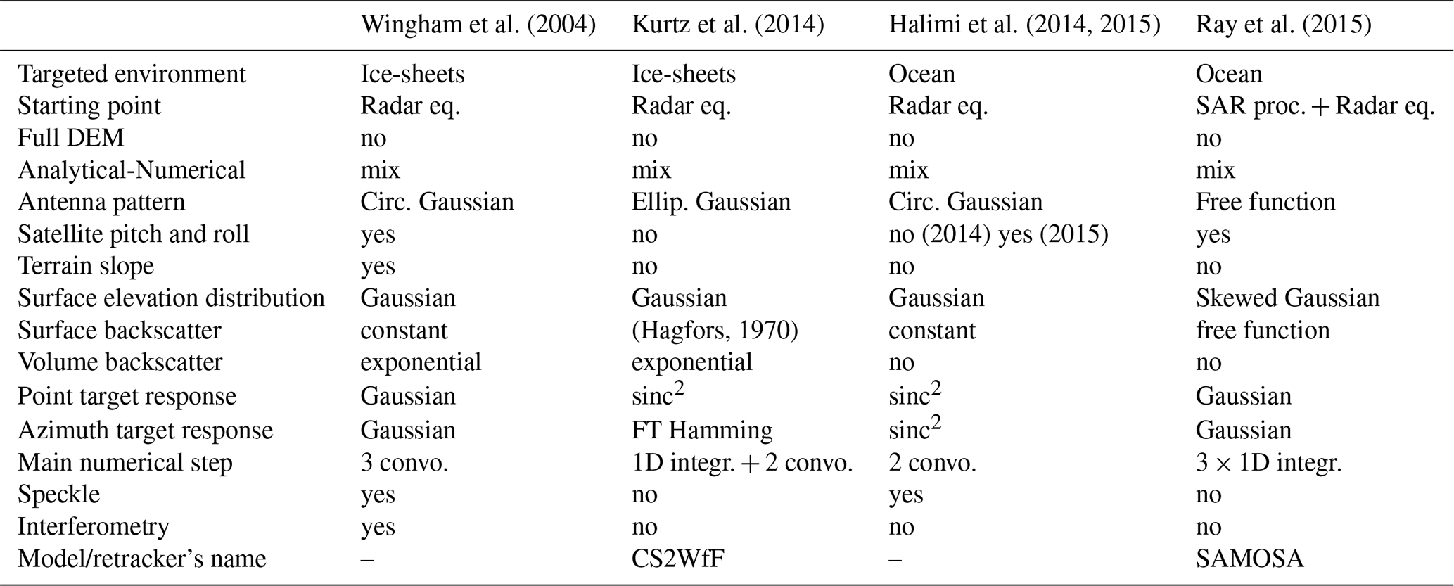
Table 2 List of more recent unfocused delay-Doppler map and waveform models with their main characteristics.

Landy et al. (2019)De Felice Proia et al. (2022a, b)Aublanc et al. (2025a)Wingham et al. (2004)

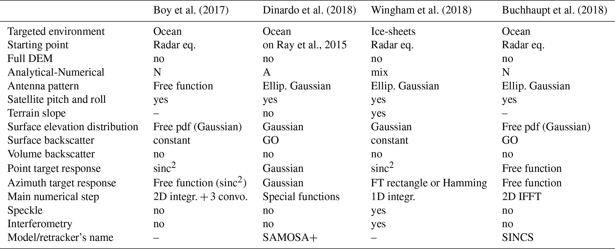
Table 3 List of unfocused delay-Doppler map and waveform models using explicit Digital Elevation Models.

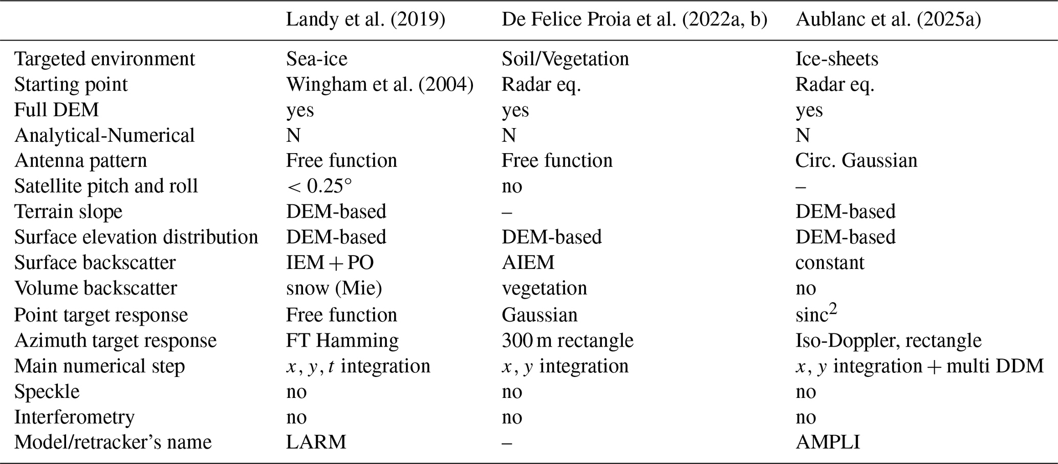
At first glance, these publications and their models appear quite different, despite all utilizing the radar equation at some stage. This is largely due to differences in notation, variable, and coordinate system choices. For instance, some use viewing angles, others prefer Cartesian coordinates on the surface. However, these differences do not affect the simulated waveform shape. Once they are accounted for, several more profound approximations remain that affect the waveform shape. These differences arise from the different considered effects (e.g. single or multiple interfaces, volume effects, terrain slope, non-circularity of the antenna, displacement of the satellite during a burst or between bursts), different choices to represent processes (e.g. the emitted compressed pulse is approximated by a Gaussian or a sinc² function) and different strategies in the analytical derivation and numerical implementation (e.g. derivation in the real domain or in the Fourier domain). These factors influence the accuracy of the waveform, the ability to assess sensitivity to geophysical parameters, and the computation time required to obtain a waveform. However, despite these differences, all these models are suitable for integration in SMRT and can be applied to cryospheric environments after appropriate adaptation, even those developed for the sea surface. The following sections delve into more details on these characteristics.

2.1 Common basis

All these models share a common foundation by using the radar equation (e.g. Brown, 1977), which relates the energy received at the antenna to the energy emitted by the same antenna (or another in the case of interferometry), summing the reflections in all the points of the surface within the footprint, and possibly including the subsurface volume. They adopt a geometrical approach to energy transport (radiative transfer) and only account for first-order scattering (i.e. single reflection at the surface or in the volume), which is certainly sufficient when the surface scattering dominates. However, in the case of snow, particularly older, coarse-grained snow, multiple scattering may be significant at higher frequencies, such as in the Ka-band (Tsang and Kong, 1980). Multiple scattering within the volume, between interfaces, and between layers and interfaces involves pathways longer than those of single scattering (Tan et al., 2015) and primarily affects the trailing edge of the waveform.

Since these models are based on energy propagation, the phase information of the electromagnetic wave is discarded, making it impossible to calculate the coherence between signals acquired in different pulses. As a consequence, these models cannot fully simulate the phase information recorded by real altimeters. Since SAR processing relies on this information and the specific pulse sequence to synthetically compress the footprint in the azimuth direction, the output of these models cannot be used as input to SAR processing algorithms. Instead, they aim to simulate both electromagnetic-surface interactions and the effects of SAR processing, and produce delay-Doppler maps as output, which can eventually be converted into waveforms by summing the maps along the Doppler dimension. Despite this limitation, they remain valuable because they are based on physical principles that incorporate the characteristics of both the sensor and the surface properties, enabling investigations of waveform sensitivity to numerous geophysical and instrumental variables.

2.1.1 SAR processing representation

Two primary approaches have been proposed for modelling SAR processing. The approach most closely aligned with UF-SAR processing was proposed by Ray et al. (2015), which first analytically calculates the signature of an individual scatterer at the surface using simplified UF-SAR equations. This leads to a bi-dimensional point target response which is then combined with the radar equation to calculate the contribution of all points within the footprint. Apart from Dinardo et al. (2018), which builds on Ray et al. (2015), all the other reviewed models assume that the effect of UF-SAR processing can be represented by a spatial convolution with a prescribed impulse function that depends on the delay (gate) and the Doppler frequency. An example of such impulse responses is shown in Fig. 1, calculated with the model described by Wingham et al. (2004) for a perfectly flat surface and Sentinel-3 characteristics in Ku-band.

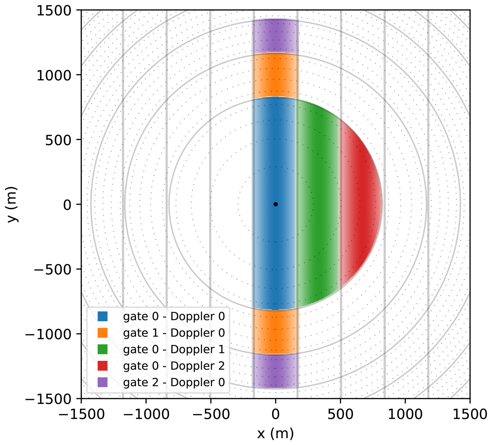
Figure 1 Impulse responses for a few gate and Doppler bin numbers over a perfectly flat surface. The weight of the response in each point is proportional to the intensity of the colour. The iso-Doppler frequency (vertical lines) and iso-range (thick circles) are represented. The thin circles mark the locations where the impulse function is effectively evaluated in Wingham04 when the time oversampling is set to 4 (the default). The antenna is pointing to the central point (black), and the satellite is transiting along the x direction (azimuth direction).

2.2 Different representations of the surface topography

Another key difference between the reviewed models lies in how they represent variations in surface elevation within the footprint. The majority (8 out of 11) represent elevation variations using an isotropic random variable Z with a known distribution (“Surface elevation distribution” in Tables 1–3). This random variable is assumed to be stationary within the footprint, meaning that the surface exhibits uniform statistical characteristics throughout. Consequently, these models cannot simulate heterogeneous terrain with spatial variations in roughness within the footprint; the roughness is assumed to be uniform, and Z is a true random variable rather than a random field Z(x,y). As a result of these approximations, the surface can be fully described by a 1D probability density function (PDF). Moreover, these models often also assume a Gaussian distribution, facilitating the analytical convolution and requiring only one parameter, the standard deviation. However, Landy et al. (2019) observed that a log-normal distribution might be more appropriate for sea-ice surfaces. This is an important consideration for any non-Gaussian target, as it affects the expected surface scattering response. For Gaussian surfaces, the local height and slope are independent (Eq. 5.5.6 in Adler and Taylor, 2009), so the surface topography effects can be included by convolving the scattering response with the elevation distribution of scatterers. For non-Gaussian surfaces, the height and slope may not be independent (Adler and Taylor, 2009), such that the surface topography-backscatter dependency cannot be accurately represented through a simple linear convolution. The bias introduced by nonuniform backscatter from a non-Gaussian surface is known as the “electromagnetic (EM) range bias” or “sea state bias” in ocean altimetry (Passaro et al., 2018).

For the models using both this statistical representation of the topography and using the uni-dimensional convolution to represent UF-SAR processing, the signal can be formulated by extending Brown's equation.

$$\begin{array}{}\text{(1)}& {\displaystyle }{\displaystyle }P\left(\mathit{\tau }\right)=\text{PDF}\left(\mathit{\tau }\right)\ast \text{FSR}\left(\mathit{\tau }\right)\ast \text{PTR}\left(\mathit{\tau }\right)\end{array}$$

to

$$\begin{array}{ll}{\displaystyle }P(\mathit{\tau },f)=& {\displaystyle }\text{PDF}\left(\mathit{\tau }\right)\ast \text{FSR}(\mathit{\tau },f)\ast {\text{PTR}}_{\text{time}}\left(\mathit{\tau }\right)\\ \text{(2)}& {\displaystyle }& {\displaystyle }\ast {\text{PTR}}_{\text{Doppler}}\left(f\right)\end{array}$$

where P(τ,f) is the power received at the antenna at time (named gate) τ and Doppler frequency f, PDF is the statistical distribution of the topography, FSR is the flat surface response, and PTR is the point target response, corresponding to the shape of the compressed pulse emitted by the altimeter for conventional altimeters. PTR_time is the equivalent of PTR, and PTR_Doppler describes the effect of UF-SAR processing. The operator ∗ denotes a convolution over time and/or Doppler frequency dimensions. The models by Ray et al. (2015) and Dinardo et al. (2018) also adopt the statistical representation of the topography, hence implementing a convolution with PDF(t) as in Eq. (2). However, the effect of the UF-SAR processing is not represented by a convolution as in the latter term in Eq. (2).

The three remaining models (Landy et al., 2019; De Felice Proia et al., 2022a; Aublanc et al., 2025a) take a radically different approach by describing the surface with a deterministic function z(x,y), commonly referred to as a Digital Elevation Model (DEM). This approach offers greater control over the surface variation properties, allowing the use of any PDF, even without stationarity, and more importantly, enabling the application of real DEMs and stacking delay-Doppler maps along the satellite trajectory, as done in a real SAR processor. This method is particularly relevant for ice sheets, where the topography within the footprint is far from uniform and strongly affects waveform shape. Complex multiple-peaked waveforms are frequent (Huang et al., 2024) and it is currently a major source of inaccuracy in estimated altimetric height (Brenner et al., 2007; Aublanc et al., 2025a). However, using a real DEM with a resolution of typically 5–10 m comes at a cost: the radar equation integration over the surface must be performed numerically, which is typically more computationally intensive than methods based on statistical representations.

The deterministic function z(x,y) can be provided on a Cartesian grid, with a recommended resolution of 5–10 m (Boy et al., 2017) and an extent covering the effective footprint (≈20 km). This approach was adopted by De Felice Proia et al. (2022b) and Aublanc et al. (2025a). Alternatively, Landy et al. (2019) employed a triangular mesh, which facilitates the calculation of the normal for each triangle, required to estimate the local incidence angle and account for variations in backscatter as a function of it. This is why Landy et al. (2019) model is referred to as a “facet-based model” and can simulate the EM bias effect.

2.3 Analytical vs. numerical approach

Another significant difference among the models lies in their approaches to calculation, particularly in the balance between analytical derivation and numerical computation. In Tables 1–3, we categorize these strategies into three types: purely analytical (A), semi-analytical (AN), and numerical (N). In practice, there is a continuum between these approaches, with some models favouring analytical derivation at the cost of substantial approximations (e.g. Dinardo et al., 2018), while others prioritize calculation precision, resulting in higher computational costs (e.g. Landy et al., 2019).

The analytical approach generally involves selecting specific shapes for the key functions in Eq. (2), such as the Point Target Response or the surface elevation PDF. The Gaussian shape usually enables tractable analytical integration. Simplifying assumptions, like treating UF-SAR processing as a uni-dimensional convolution, can also make the problem more manageable. However, this assumption is not strictly necessary; for example, Ray et al. (2015) and Dinardo et al. (2018) have advanced the analytical development without relying on such simplification.

Numerical methods become essential when using a DEM as input, as previously mentioned. However, this is not the only reason. For instance, Buchhaupt et al. (2018) opted for an analytical development of the functions in Eq. (2) in the Fourier domain, transforming the convolution into multiplication, and ultimately relied on numerical inverse Fast Fourier Transform (FFT) to convert results back to the real space. In this case, the computational cost is minimal due to the FFT algorithm's efficiency, making this model more efficient overall than some semi-analytical models that rely on traditional (i.e. non-FFT) numerical integration.

Both approaches offer complementary advantages. The analytical approach is better suited for running intensive sensitivity analysis, to understand how the altimetric signal varies with the various parameters and for developing physical retracker algorithms that fit observed waveforms across a large parameter space without lookup tables. In contrast, DEM-based, numerically intensive models are more effective as forward models for exploring the effects of complex terrain (Aublanc et al., 2025a). However, this does not preclude the use of such models in retrackers, as demonstrated by Aublanc et al. (2025a) in their retracker named AMPLI.

In the following sections, we examine other less prominent differences among the models.

2.4 Antenna gain (G)

The antenna gain pattern describes the angular response of the altimeter antenna and particularly influences waveform decay.

In analytical models, the antenna gain pattern is typically assumed to decrease with a Gaussian shape as a function of the angle or the sine of the angle (both are nearly equivalent for small angles as relevant in space-borne altimetry). This assumption effectively represents the main lobe of the antenna gain (Brown, 1977), but it completely neglects the secondary lobes. Early models (e.g. Halimi et al., 2014) also assumed a circular antenna, leading to an axisymmetric pattern. In this simple case, the Gaussian shape is characterized by a single parameter – typically the beamwidth angle (around 1°) – where the gain decreases by 3 dB (nearly a factor of 2). However, with the introduction of the elliptical antenna onboard CryoSat, this simple representation became inadequate. Under the assumption of the separability of the pattern in the across and along track directions, a more complex Gaussian pattern – decreasing at different rates in the along-track (1.06° for CryoSat-2) and cross-track (1.1992°) directions – was adopted. The Gaussian assumption remains convenient because it is well-suited for analytical calculations. For this reason, complex antenna patterns can be described as a sum of Gaussian assumption, as in Buchhaupt et al. (2025), an advanced version of Buchhaupt et al. (2018).

Incorporating the actual antenna diagram, including its irregularities and secondary lobes, can significantly enhance model accuracy (Boy et al., 2017). This approach requires numerical integration of the tabulated gain function. For example, (Ray et al., 2015) do not require any particular assumption for the gain function, making their model adaptable to any antenna diagram. Additionally, their calculation framework is devised so that this integration involves only sensor parameters, which can be pre-calculated. This makes their model efficient and well-suited for use as physical retrackers. Boy et al. (2017) and De Felice Proia et al. (2022a) also use the measured antenna pattern to achieve greater precision.

2.5 Satellite pitch and roll

Most models, especially the most recent ones, explicitly account for the satellite's imperfect attitude, which leads to antenna mispointing. This factor significantly affects the analytical expressions, as seen in Eq. (26) in Buchhaupt et al. (2018). The impact of the antenna mis-pointing on the waveforms is illustrated in Ray et al. (2015) in Figs. 9 and 10 with 0.2° of pitch and roll, respectively. Although Halimi et al. (2014) do not consider mis-pointing, subsequent work (Halimi et al., 2015, not listed in Table 1) introduces this effect through an integral that incorporates a series of Bessel functions.

2.6 Point target response (PTR) or compressed pulse shape

The PTR_time represents the shape of the compressed pulse, typically characterized by a sinc² function (Chelton et al., 1989) or better, using the real PTR of the instrument obtained from the internal calibration in order to increase the retracking performance. However, the analytical integration involving these functions is generally intractable, leading many models to adopt a Gaussian approximation instead (Brown, 1977; Dinardo et al., 2018). It is indeed possible to fit a Gaussian to the ${\sin }^{\mathrm{2}}\left(Nx\right)/{\sin }^{\mathrm{2}}\left(x\right)$ and sinc² functions by neglecting their secondary oscillations. Yet, there is no single method for this fit, resulting in various amplitudes proposed in the literature, ranging from 0.425 (Brown, 1977) to 0.513, as reported by MacArthur (1978) and cited by Gommenginger et al. (2010). MacArthur (1976) suggested a value of 0.443, while our own fit yielded a lower value of 0.36. These different options are available in SMRT.

It is worth noting that any model limited to a Gaussian pulse can in principle be extended by first calculating the delay-Doppler map without the PTR_time – that is, by setting the Gaussian width zero – and then reintroducing the PTR_time via numerical convolution. This approach may introduce numerical errors (due to the zero-width Gaussian) and increase computational cost, depending on the models.

2.7 Azimuth point target response

The effect of UF-SAR processing in the azimuth direction is typically represented by a response function (PTR_Doppler) in the majority of models, analogous to the time domain. Although the terminology and equations vary across different studies, this response ideally follows a ${\sin }^{\mathrm{2}}\left(Nx\right)/{\sin }^{\mathrm{2}}\left(x\right)$ function (i.e. the Fourier Transform of a sampled rectangular signal), sometimes modified by the influence of a Hamming tapering window if it was applied during UF-SAR processing. The Hamming window aims to reduce the secondary lobes by apodisation at the expense of a slightly decreased resolution in the along-track direction, e.g. from 300 to 450 m for the CryoSat-2 mission. Some studies employ the sinc² function instead (i.e. Fourier Transform of a rectangular signal), corresponding to the previous case when N, the number of Doppler frequencies is very large. At last, for analytical tractability, many models also employ a Gaussian approximation for the response function (e.g. Kurtz et al., 2014). This approximation is particularly justified and effective when the Hamming window is applied for the UF-SAR processing, as it significantly reduces secondary lobes (Ray et al., 2015) compared to the untapered ${\sin }^{\mathrm{2}}\left(Nx\right)/{\sin }^{\mathrm{2}}\left(x\right)$ function. For sensors with a low number of Doppler frequencies N such as Sentinel-3 at C-band (N=2), only models using ${\sin }^{\mathrm{2}}\left(Nx\right)/{\sin }^{\mathrm{2}}\left(x\right)$ are suitable. For the other existing space-borne sensors with N=64, the sinc² and Gaussian approximations are acceptable.

2.8 Surface elevation probability density function (PDF)

In models that use a statistical representation of surface elevation, the vertical distribution is typically described by a probability density function (PDF). This function is often assumed to follow a normal distribution, which is commonly used in various fields to represent rough surfaces due to its simplicity and the tractability it offers for analytical calculations. However, Ray et al. (2015) introduced a skewed Gaussian distribution to accommodate more general cases, while Landy et al. (2020) strongly suggested that a log-normal distribution is more appropriate for modelling sea-ice surfaces. The disadvantage of using a more complex distribution to represent the surface elevation is that each distribution parameter adds another dimension to the solution space for physical retracking.

The Fourier domain-based model proposed by Buchhaupt et al. (2018) is not limited to normal distributions. In fact, it can efficiently handle any distribution that has a known analytical form in Fourier space. Additionally, as mentioned for the point target responses (PTR), the models that assume a normal distribution can, in principle, be adapted to other distributions by applying numerical convolution with the PDF.

2.9 Terrain slope

The terrain slope at the footprint-scale (>10 km) is particularly relevant for ice sheets, which is why it is explicitly accounted for in some models using the statistical representation of the surface elevation and dedicated to this type of surface (e.g. Wingham et al., 2004, 2018). Despite this useful addition, using a real Digital Elevation Model (DEM) as input can implicitly incorporate this large scale terrain slope through the DEM data as well, and many more details (Aublanc et al., 2025a). Note also that a constant terrain slope can be approximated by adjusting the pitch and roll parameters (with opposite sign).

2.10 Surface and volume backscatter

The simplest approach for backscatter modeling is to only consider the surface echo and assume a constant backscatter value, independent of the incidence angle as in Halimi et al. (2014) and Wingham et al. (2018). However, it is well established that the reflectivity of a smooth surface decreases sharply with increasing incidence angle, i.e. the angle between the radar beam and the surface normal, which is vertical for a horizontal surface. Although the incidence variations seem small in altimetry (<1–2°), they are large enough to have a first-order impact on the trailing edge of the waveform.

Assuming a Gaussian decrease in backscatter with incidence angle is advantageous for analytical tractability and aligns with the physics of the Geometrical Optics approximation (Tsang et al., 2000; Chen et al., 2003). However, this theory is only applicable to very rough surfaces, where the Root Mean Square (RMS) height and the horizontal correlation length are much larger than the wavelength. Other empirical or physical rough surface scattering models can be used. For example, Dinardo et al. (2018) assumes a linear dependency between backscatter and incidence angle. In contrast, some models, such as Ray et al. (2015), rely on numerical integration and thus can handle any backscatter function, including the antenna gain. Landy et al. (2019) and De Felice Proia et al. (2022a) incorporate the Integral Equation Model (IEM, Fung, 1994) or its variants (e.g. Chen et al., 2003; Brogioni et al., 2010), which are valid for a wide range of moderate roughness conditions. Landy et al. (2019) accounts for the local incidence angle in each facet of the DEM, which is crucial to simulate the EM bias caused by skewed slope distributions, for instance, when flatter, more reflective facets are more likely at the base of the terrain rather than equally distributed (Tran et al., 2010).

Volume scattering is less commonly addressed in the models reviewed here, primarily because many were developed for oceanic applications, where microwave penetration beneath the surface is negligible. However, this is not the case for dry snow or ice. The simplest approach to account for volume scattering is to assume a homogeneous semi-infinite layer with user-prescribed empirical values for the backscatter and attenuation rates (Wingham et al., 2004). For sea ice, Landy et al. (2019) assumed a finite single snow layer overlying the ice interface. Snow scattering and absorption were calculated using Mie theory (Mie, 1908). However, Mie theory is not suitable for snow due to its high density (Tsang et al., 1985; Picard et al., 2022c). In De Felice Proia et al. (2022a), the volume is discretized into cells, allowing for a fully 3D calculation of volume backscatter, potentially enabling the description of complex medium structures.

2.11 Speckle and stacking

Radar measurements are inherently influenced by a physical fluctuation known as speckle, caused by wave interference from different scatterers within the radar footprint. The models reviewed here, which are based on the radar equation, describe only the propagation of the power and do not account for the wave nature, thereby implicitly averaging out the effects of speckle. However, it is possible to simulate speckle by ad hoc addition of a random noise in each cell of the delay-Doppler map. This noise is typically modelled using an exponential distribution, as described by Wingham et al. (2004). When averaging the delay-Doppler map to compute the waveform, this noise distribution approximates to a gamma distribution (Halimi et al., 2014) under stationarity approximation, which, with a large number of Doppler beams, tends to resemble a Gaussian distribution (Wingham et al., 2004). However, this approximation is in general not valid for a moving target, as on the ocean (Buchhaupt et al., 2023) or for complex terrains, as on the ice-sheet margins (Aublanc et al., 2025a). The averaging process (stacking) is more complex and advanced strategies can be deployed. This is not considered in our new development.

2.12 Interferometry

The model presented by Wingham et al. (2004) provides equations for two antennas separated by a baseline, making it suitable for SARIn altimetric simulation, as described by Rosen et al. (2000). Although this capability is an asset, it is not explored in this review.

2.13 Computation time

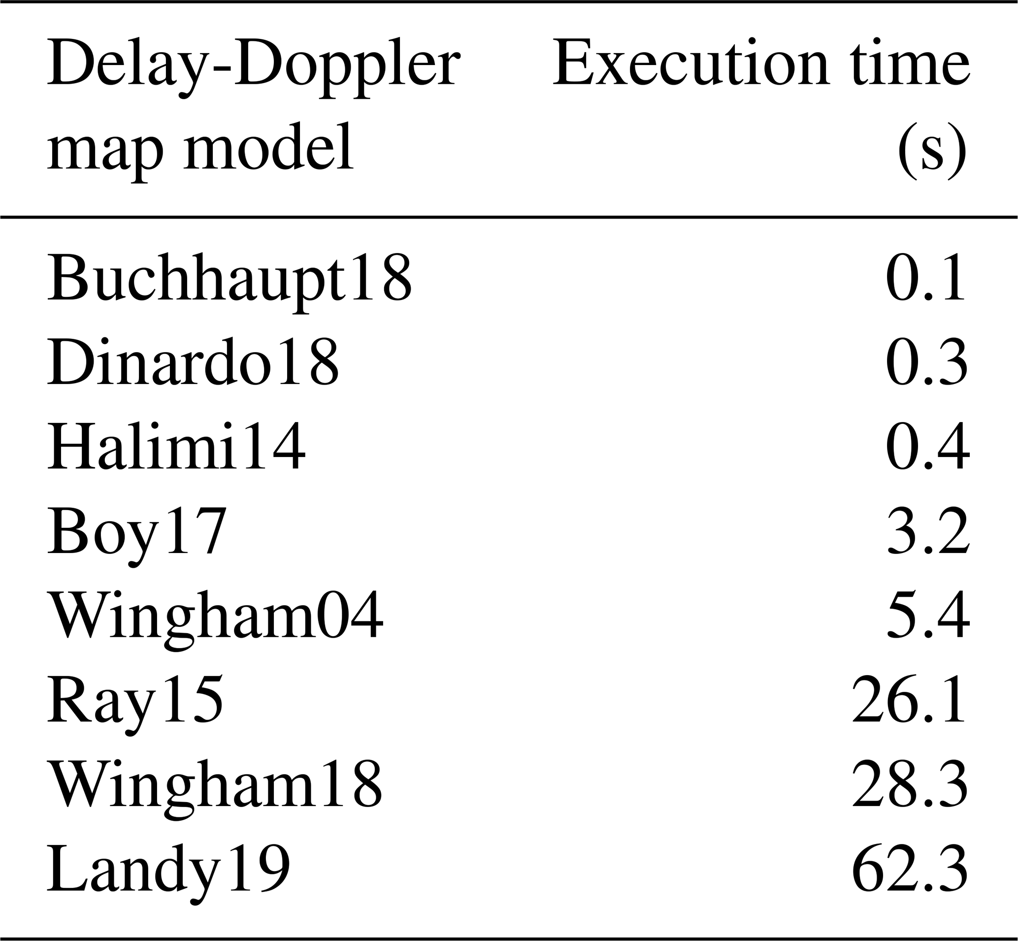
The model developed by Landy et al. (2019) is the most computationally intensive for three reasons. First it performs the summation on the x,y grid of the surface (as Boy et al., 2017) instead of relying on analytical or semi-analytical integrations. Second, it accounts for satellite motion during the acquisition of the 64 beams, a unique feature among the models. However, this requires 64 distinct summations over the x,y grid. At last, the convolution with Point Target Response (PTR) in time is performed using basic numerical integration in the original model. At first glance, choosing the sinc² function imposes such an ineffective approach. However, we found that the “sinc² transform” proposed by Greengard et al. (2006) is appropriate to perform the specific convolution with this PTR. This transformation, by leveraging the Fast Fourier Transform (FFT), is significantly more efficient. Moreover, this transformation was implemented in a Python package (https://github.com/gauteh/fsinc, last access: 3 December 2025) that also accommodates non-uniformly spaced samples. This is essential given that the summation over the grid involves irregularly spaced ranges. The use of this transformation significantly accelerates computation by a factor of 50–100 based on our implementation (not tested in the original code). Nevertheless, our implementation of Landy et al. (2019) model remains the most computationally expensive despite this improvement.

In contrast, the models by Dinardo et al. (2018) and Buchhaupt et al. (2018) are the most computationally efficient. The former relies solely on analytical functions. Despite requiring the unconventional Exponentially Scaled Modified Bessel function, it benefits from an efficient implementation directly available in the mainstream SciPy Python package (Virtanen et al., 2020). The second model is mostly numerical but was designed for fast execution, suitable for physical retracking. It applies Fourier transforms to convert convolutions into products, but unlike other models, it directly derives analytical expressions for the flat impulse response and PTRs in Fourier space, thereby avoiding several FFT calculations. This approach results in a substantial reduction in computational cost. The other models fall between these two extremes, employing either slower integration methods or faster FFT-based convolutions.

The time to compute one delay-Doppler map is given in Table 4. It is important to note that detailed benchmarking of these models is beyond the scope of this review, as performance can vary significantly with implementation details and hardware. Additionally, our primary objective being to provide a readable Python implementation of the models that closely adheres to the published equations, aggressive code optimizations were excluded.

Table 4 Indicative execution times to compute one delay-Doppler map with the eight models implemented in SMRT. The times are indicative. Not all the models have been optimized to the same degree.

2.14 Summary

The delay-Doppler models reviewed in Sect. 2, despite sharing the common aim of predicting waveforms from radar and surface characteristics, exhibit a wide range of approaches. This diversity is multi-dimensional as illustrated by the numerous rows in Tables 1–3. Some of these dimensions are fundamental, driving the model derivation and features (e.g. how to represent the topography), while others are specific to a study and could easily be modified (e.g. whether to take terrain slope and tilt into account). Nevertheless, while the most recent models are generally more capable than the earliest ones, there is no unique best model, mainly because they target different applications. For this reason, eight of these models have been implemented in SMRT version 1.7 (Picard, 2026a), allowing users to easily compare them and select the most suitable for their application. The list is: Wingham04, Halimi14, Ray15, Boy17, Buchhaupt18, Dinardo18, Wingham18, and Landy19.

3 Implementation of SAR altimetry in SMRT

3.1 General algorithm

The altimetry module, newly implemented in SMRT, aims to simulate UF-SAR processing and to output Doppler maps given the scattering and extinction properties (K_s(z) and K_e(z) respectively) and the effective permittivity ϵ_eff(z) of each layer, and the snowpack interface reflectivity and transmittivity, as calculated in other pre-existing SMRT modules. Instead of developing a complete module for each DDM model, we first identified the parts of the altimetric computation that are common across models and those that are specific to each model.

The key assumption is to limit the computation to first–order scattering, which implies independence between the different scattering mechanisms. It follows that the total power P(τ,f) received by the sensor (i.e. the DDM) is the sum of the contributions from each elementary layer and each interface independently. In general, the role of the DDM models is to compute the power $\mathrm{\Pi }(\mathit{\tau },f,{\mathit{\sigma }}^{\mathrm{0}})$ received as a function of delay τ and Doppler frequency f, given the backscattering coefficient σ⁰(θ) of a surface. The other existing modules in SMRT compute the backscatter ${\mathit{\sigma }}_{\text{interface}i}^{\mathrm{0}}\left(\mathit{\theta }\right)$ of each interface i (i.e. surface, internal inter-layer interfaces, and substrate) and the profile of backscatter ${\mathit{\sigma }}_{\text{volume}}^{\mathrm{0}}(z,\mathit{\theta })$ coming from the layers. In addition we compute the delay and attenuation at depth z relative to the surface, represented by the generalized function Δ(z,τ) using the extinction K_e(z), transmittivity of the interfaces and the wave speed deduced from the refractive index $\sqrt{{\mathit{ϵ}}_{\text{eff}}\left(z\right)}$. It follows that:

$$\begin{array}{ll}{\displaystyle }P(\mathit{\tau },f)=& {\displaystyle }\underset{z}{\int }\mathrm{\Pi }(\mathit{\tau },f,{\mathit{\sigma }}_{\text{volume}}^o(z,\mathit{\theta }\left)\right)\ast \mathrm{\Delta }(\mathit{\tau },z)\mathrm{d}z\\ \text{(3)}& {\displaystyle }& {\displaystyle }+\sum _i\mathrm{\Pi }(\mathit{\tau },f,{\mathit{\sigma }}_{\text{interface}i}^{\mathrm{0}}(\mathit{\theta }\left)\right)\ast \mathrm{\Delta }(\mathit{\tau },z_i)\end{array}$$

where the integral applies to the whole snowpack and i runs over the interfaces (surface and inter-layer interfaces). A second key assumption is considering volume backscatter is virtually independent of the zenith angle within the footprint of near-nadir altimeters (typical range ≈1–3°). This simplification is not applicable to the interfaces because their backscatter varies rapidly for off-nadir angles, especially the coherent backscatter component. With this simplification, the integral over the snowpack becomes a linear convolution (Eq. 17 in Wingham et al., 2004) yielding:

$$\begin{array}{ll}{\displaystyle }P(\mathit{\tau },f)=& {\displaystyle }{\mathit{\sigma }}_{\text{volume}}^{\mathrm{0}}\left(z\right)\ast \mathrm{\Delta }(\mathit{\tau },z)\ast \mathrm{\Pi }(\mathit{\tau },f,\mathrm{1})\\ \text{(4)}& {\displaystyle }& {\displaystyle }+\sum _i\mathrm{\Pi }(\mathit{\tau },f,{\mathit{\sigma }}_{\text{interface}i}^{\mathrm{0}}(\mathit{\theta }\left)\right)\ast \mathrm{\Delta }(\mathit{\tau },z_i).\end{array}$$

Hence, the computation can be performed in three independent steps: (1) calculate the vertical profile of volume backscatter and the backscatter values of each interface, (2) compute the delay-Doppler maps for each interface ${\mathrm{\Pi }}_{\text{interface}i}(\mathit{\tau },f,{\mathit{\sigma }}_{\text{interface}i}^{\mathrm{0}}(\mathit{\theta }\left(\mathit{\tau }\right)\left)\right)$ and for the volume ${\mathrm{\Pi }}_{\text{interface}i}(\mathit{\tau },f,\mathrm{1})$, (3) combine the vertical profile of backscatter and the DDMs to provide the final DDM P(τ,f) using Eq. (4) and eventually the waveforms (Fig. 2) as follows.

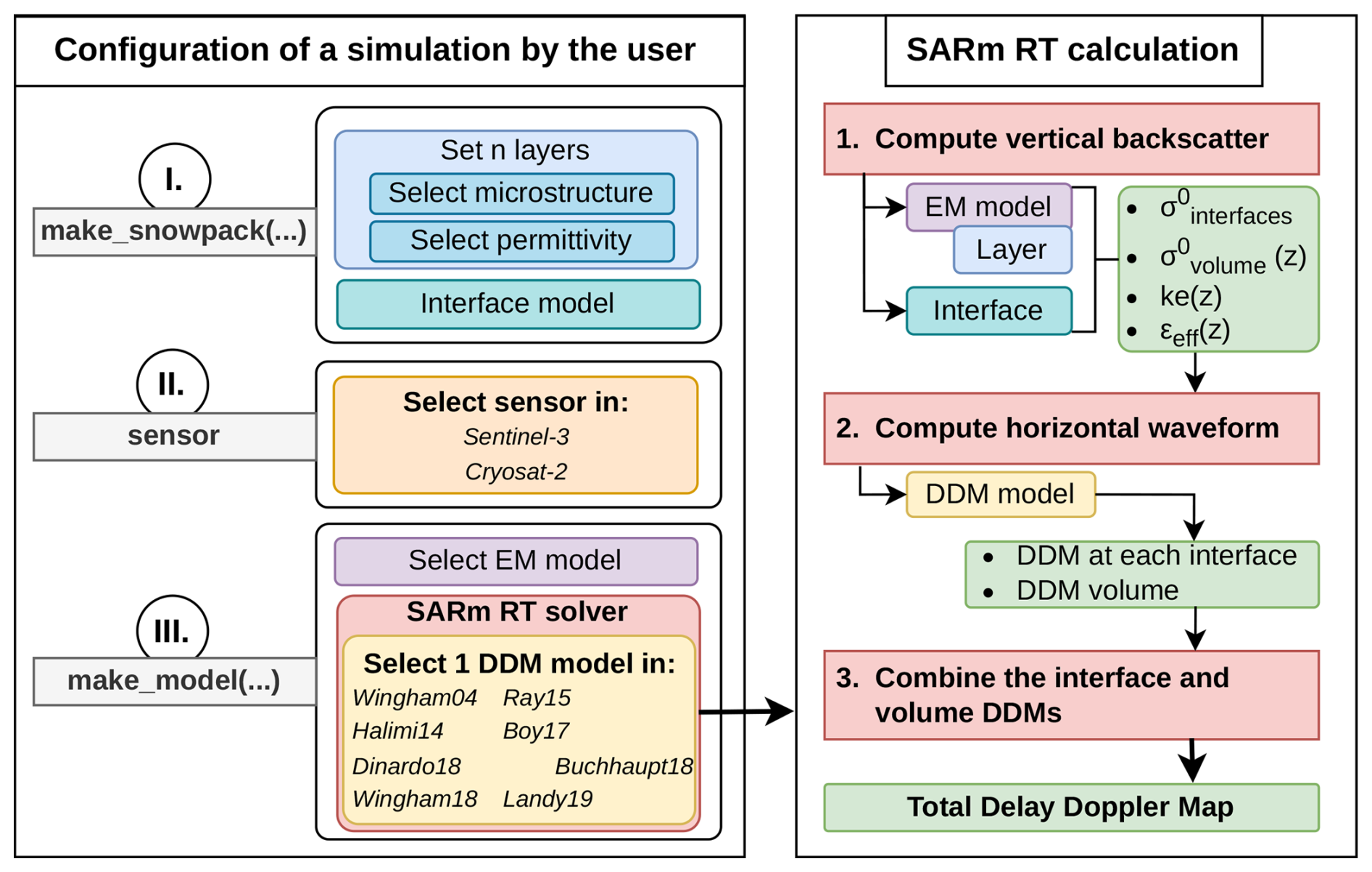
Figure 2 Workflows of the configuration of the model by the user and of the calculation performed in the new Nadir SAR RT solver. Bold face underlines the new components added in SMRT for the present study. Italic face represents the available options.

Step 1 computes the backscattering coefficients of each layer and each interface according to the type of medium (snow, ice, …) and its properties, and the electromagnetic theories (Improved Born Approximation, Geometrical Optics Approximation, …) selected by the user (Fig. 2). This step uses existing SMRT functions that are not specific to altimetry and were developed in early stages of SMRT development (Picard et al., 2018). Only the coherent backscatter (Sect. 3.2) was added specifically for this study. The volume backscatter of each layer is then interpolated onto a sub-grid, regular in propagation time τ (“gate”) following Larue et al. (2021), leading to a backscatter as a function of delay ${\mathit{\sigma }}_{\text{volume}}^{\mathrm{0}}\left(\mathit{\tau }\right)$. In the LRM altimetry module, the interface backscatter was treated similarly to the volume backscatter because the authors assumed that all interfaces had the same roughness and the same angular variations in backscatter. However, this assumption is not satisfactory especially for flat surfaces with peaked backscatter, so Π depends on the diagram of backscatter σ⁰(θ). In the SAR altimetry module, each interface can have a different roughness, which requires computing and storing the backscatter for each interface at all incidence angles within the illuminated footprint. The output of step 1 is thus the volume backscatter time series ${\mathit{\sigma }}_{\text{volume}}^{\mathrm{0}}\left(\mathit{\tau }\right)$ and a list of backscatter ${\mathit{\sigma }}_{\text{interface}i}^{\mathrm{0}}\left(\mathit{\theta }\right)$ for all interfaces.

Step 2 calls the user-selected DDM model (Fig. 2). Our approach for implementing the DDM models was to follow the equations of the original studies as closely as possible. Most equations in the code are traceable to their respective studies. Nevertheless, some models required minor adaptations. Boy et al. (2017) does not provide sufficient equations; the gaps were inferred from Halimi et al. (2014). In the case of Landy et al. (2019) the full model was not implemented, as SMRT already included many of the necessary components (e.g. interface and volume backscatter). As with many other modules in SMRT, these DDM modules are fairly independent of the rest of the code and can be tested and used outside of SMRT. New DDM models can also be added easily thanks to the plug-in framework.

In this step 2, the selected DDM model is called for each value of interface roughness, providing a DDM for each interface $\mathrm{\Pi }(\mathit{\tau },f,{\mathit{\sigma }}_{\text{interface}i}^{\mathrm{0}}(\mathit{\theta }\left)\right)$ along with the delay and attenuation generalized function Δ(τ,z_i) at the depth of the interface z_i. For the models using an explicit DEM (Boy17 and Landy19), the backscatter dependence on incidence angle for each interface is accounted for at this stage, since the local incidence angle can differ across facet slopes and orientations. In addition, a DDM is calculated for the volume ${\mathrm{\Pi }}_{\text{volume}}(\mathit{\tau },f,\mathrm{1})$ assuming volume scattering angular dependency is negligible over the range of incidence angle typical of altimeters (0–2°). The output of this step is a list of DDMs. These DDMs are calculated with a finer sampling interval in the time and Doppler dimensions to reduce numerical errors in the integrations and Fourier transforms. This results in oversampled DDMs compared to those DDM produced for altimeters (e.g. 64 bins in Doppler and 128 in time for Sentinel-3). An oversampling factor of 4 in both dimensions is typically sufficient for most models. This value is adjustable by the user. The final output DDM is optionally downsampled to match the real sensor's resolution. Figure 1 illustrates where the calculation of the impulse function is effectively performed in the case of Wingham04 (dotted circles), with an oversampling of 4 in the time dimension.

In this step 2, the slant range correction (a.k.a delay migration) is part of the analytical formulation from some models, yielding directly the corrected DDM. However, in other cases (Halimi14, Wingham04, Boy17, Landy19), the model first computes the uncorrected DDM, and we then migrate each cell in delay, with a left translation as depicted Fig. 3. The delay depends on the square of the Doppler frequency f as ${\mathit{\tau }}_{\mathrm{0}}\left(f\right)=f^{\mathrm{2}}\mathit{\alpha }H{\mathit{\lambda }}^{\mathrm{2}}/\left(\mathrm{8}{V}^{\mathrm{2}}\right)$ (Eq. 7 in Raney, 1998) with α the Earth curvature correction, H and V the satellite altitude and velocity, and λ the radar wavelength. This ensures that, in the slant range corrected DDM, the echoes for all the Doppler frequencies are aligned at the range of the zero-Doppler echo (dark green line) by compensating for the additional range sensed at different along-track distances from the target on ground (dark red parabola).

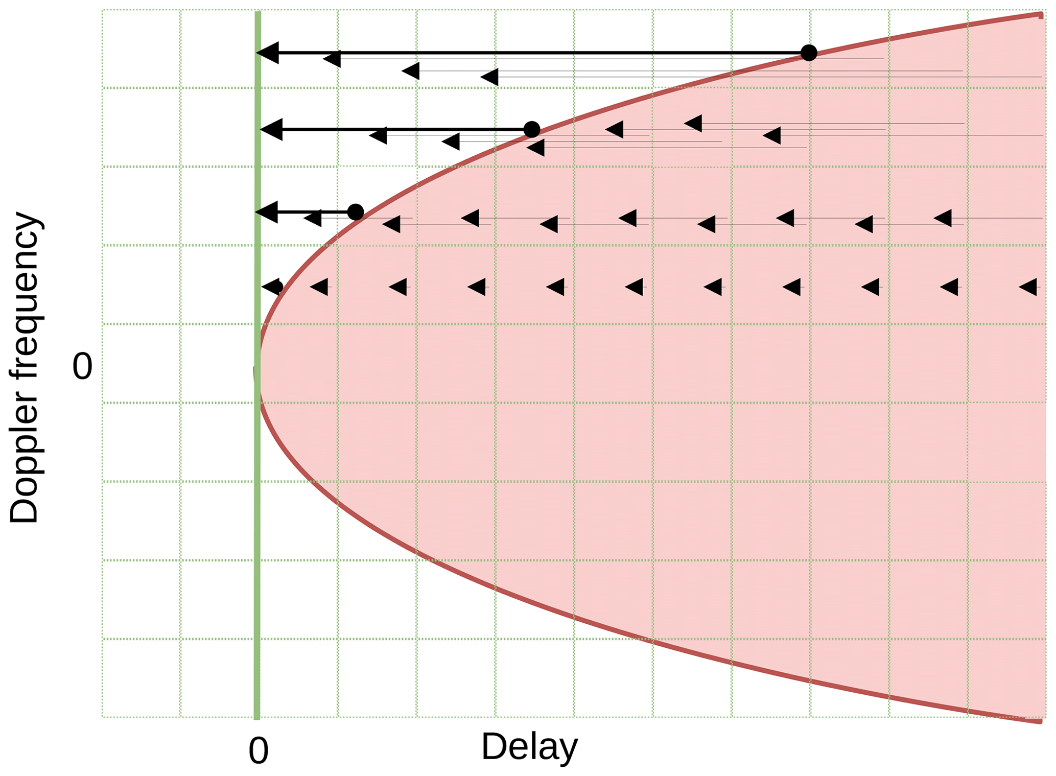
Figure 3 Schematic of the slant range correction of a delay-Doppler map. Each cell is migrated according to a delay that increases with the square of the Doppler frequency.

The third step combines the backscatter σ⁰ and DDMs Π using Eq. (4). This step returns the final DDM P(τ,f). Optionally, the terms in Eq. (4) can be returned separately (called volume DDM and interface DDM hereinafter) to enable comparison of the different contributions.

Steps 1 and 3 are common to all DDM models and implemented in the module “nadir_sar_altimetry”, while step 2 is implemented in independent modules (the files in the directory “delay_doppler_model”) that provide the Π function, one for each DDM model.

3.2 Coherent backscatter

Backscatter from a rough surface is commonly composed of a diffuse component and a coherent one (Voronovich and Zavorotny, 2017). The latter is only significant in the specular direction (also known as quasi-specular reflection). For this reason, incoherent backscatter is the only significant component in monostatic side-looking radars such as scatterometers and Synthetic Aperture Radars, and all existing SMRT functions neglect coherent backscatter. However, in nadir-looking altimetry, the specular direction is vertical, and coherent backscatter can become significant at near-nadir angles in the first time gates, known as the Fresnel region.

A specificity of coherent backscatter is to depend not only on surface roughness but also on the altitude of the sensor (Drinkwater, 1991; De Rijke-Thomas et al., 2023) when the angle subtended by the coherent scatterers at the surface is not small compared to the antenna beamwidth (Fung and Eom, 1983). For SAR altimeters, “antenna beamwidth” is understood to be the pulse-limited, focused beamwidth, which is very small (300 m in the Doppler direction). Similarly, for rough surfaces, “coherent scatterers” are understood as objects of size comparable to the correlation length, typically less than a meter. It results in the coherent backscatter having a strong impact on the interpretation of differences between in-situ radar and airborne altimeters. Space-borne sensors are only concerned when the surface is flat and smooth, such as on sea ice (De Rijke-Thomas et al., 2023).

A coherent backscatter formulation was added directly in the “nadir_sar_altimetry” module, following (Eq. 6, Fung and Eom, 1983). This approximation is considered valid for a wide range of surface roughness (Voronovich and Zavorotny, 2017).

4 Materials and Method

An assessment of the new SAR altimetry module was performed in Antarctica at 18 sites using in-situ measurements to drive SMRT (Sect. 4.1) and compared with Sentinel-3 Level 2 data (Sect. 4.2). The procedure to conduct the simulations and optimization is described.

4.1 In-situ measurements in Antarctica and ancillary data

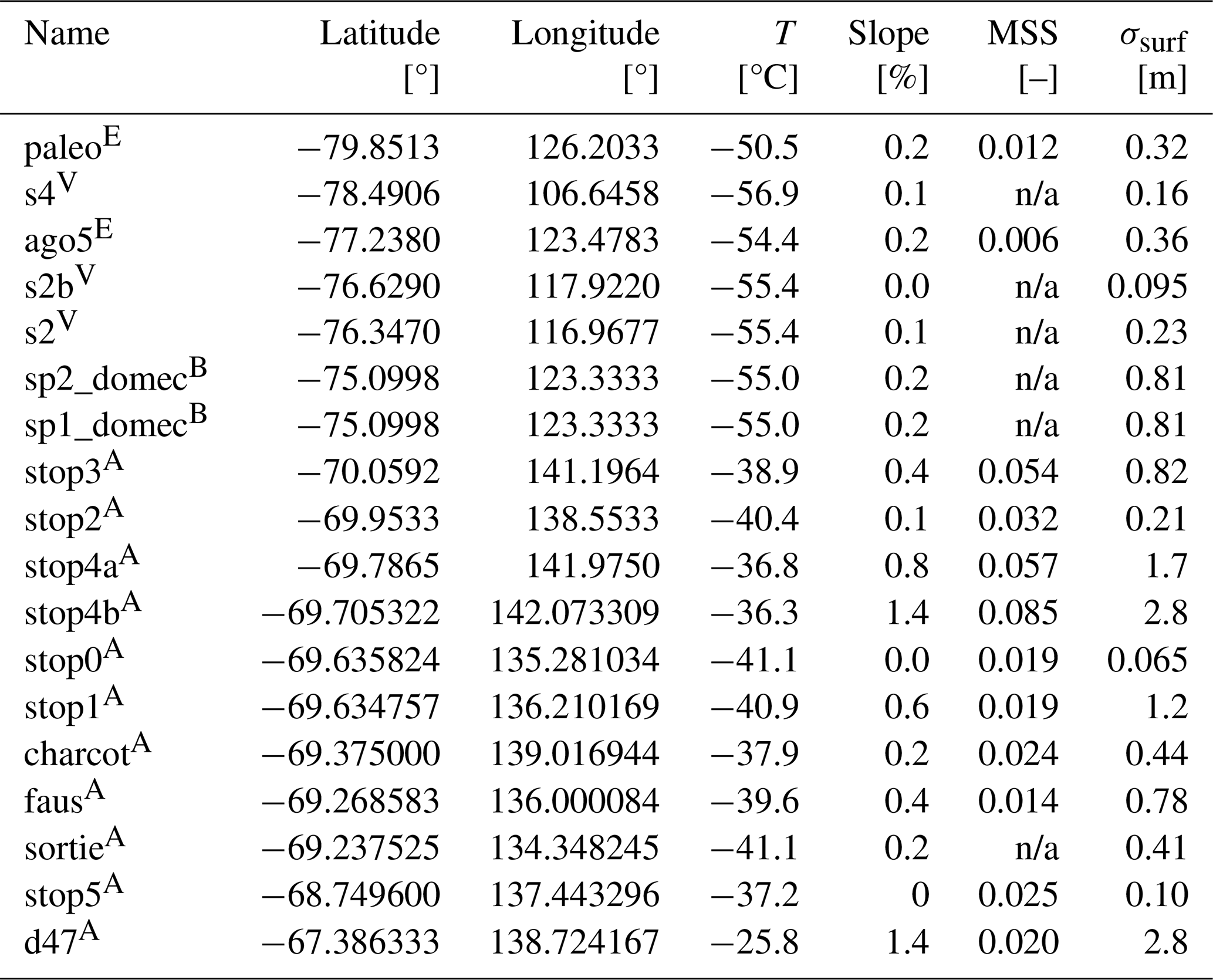
In-situ measurements relevant to perform microwave simulations have been collected through several intensive campaigns in Antarctica, namely Vulnerability of ANtarctic Ice SHeet and its atmosphere (VANISH) in 2012, BI-POle in 2012 (BIPOL), Accuracy of the Surface Mass balance of Antarctica (ASUMA) in 2016, and East Antarctic International Ice Sheet Traverse (EAIIST) in 2019. The visited sites are reported in Table 5 with their main characteristics. Most of these data were already used in previous work (Larue et al., 2021; Picard et al., 2022b) where detailed information is provided. Only a brief description is provided here.

Table 5 List of the Antarctic sites used for the assessment of the new SAR module: coordinates, measured annual temperature (T, in Celsius degrees), REAM slope (in a circle of 700 m), Mean Square Slope (MSS), large scale roughness (σ_surf, in meters). The letters in superscript indicate the campaign (A = ASUMA, B = BIPOL, E = EAIIST, V = VANISH).

In a first set of simulations, SMRT was driven with the measured vertical profiles of density, layer thickness, temperature, Specific Surface Area (SSA), surface roughness, and height distribution. At every site except VANISH, a ≈8 m core was extracted with a 10 cm diameter drill and processed on-site in a cold laboratory. Density was measured on ≈10 cm long slices. Each slice is represented as a layer in SMRT, with its measured thickness. Specific surface area (SSA) was continuously measured along the core side using the Alpine Snowpack Specific Surface Area Profiler (ASSSAP) (Arnaud et al., 2011), and averaged over each layer. The SSA and density profiles were then extended to 100 m depth by repeating the last 1 m of the ≈8 m measured profiles. A linear trend estimated over the measured profile was applied to the density to simulate the densification. This rough approximation has little impact because the altimetric signal usually comes from the upper part, where measurements were actually taken for most sites. The snow temperature was measured with a Pt100 sensor at the bottom of the drilled hole for 24 h. At this depth, the temperature is close to the annual mean temperature. For the simulations, the temperature profile was assumed uniform. Larue et al. (2021) assessed the impact of seasonal temperature variations.

The protocol applied during the earliest campaign, VANISH, was less elaborate. The cores extracted in January 2012 were shipped back to France and cut into 10 and 5 cm pieces at S2 and S4, respectively, in July 2012, in a cold chamber, to measure density and SSA.

Key measurements for altimetry are the characteristics of the surface roughness at the radar wavelength scale and the large scale height distribution within the footprint. Both are related to height variations of the surface, but differ in the spatial scales. The former (hereinafter called radar-scale roughness) controls the backscatter intensity of the surface (and the interlayer interfaces), while the latter (hereinafter large scale roughness) controls the spread of the delay of the echo and influences the local incidence angle. The radar-scale roughness is quantified by the Mean Square Slope and was estimated at some of the sites (Table 5) using a centimetre-resolution DEM of 5 m×5 m areas. The technique uses manual photogrammetry with ground-level photographs. The measurement protocol and processing are detailed in Larue et al. (2021). The large scale roughness, quantified by the standard deviation of height (σ_surf), was obtained at each site using the Reference Elevation Model of Antarctica (REMA) tiles at 2 m resolution (Howat et al., 2022). The selected area was a 700 m diameter circle around the in-situ measurement point. These data are reported in Table 5.

4.2 Sentinel-3 altimetric waveforms

For Ku-band (and independently for C band), the closest 20 Hz waveform of each site was extracted from the BC-005 ESA Land Ice Thematic Products (Aublanc et al., 2025b) after discarding the low quality waveforms (“waveform_qual_ice_20_Ku” parameter different from 0)

The waveforms were scaled with the parameter “scale_factor_20_Ku” (and C, respectively, for the Ku and C band), also provided in the L2 product. This operation is necessary to enable cross-site comparison of waveform amplitudes. However, it is not sufficient to obtain absolute power due to the lack of absolute calibration data. Therefore, the comparison with SMRT can only be relative. Larue et al. (2021) addressed this issue by estimating a single factor α(f,S) for each band f and sensor S to scale all SMRT simulations at all sites to match the observations. Using this normalization factor, the site-to-site amplitude variations between the observations and the model are preserved and are safely comparable, while the absolute values are meaningless.

4.3 Setup of the SMRT Simulations

The description of the snowpack for the Antarctic simulations follows the theoretical approach recently introduced by Picard et al. (2022b). This new approach calculates the Porod length l_p using in-situ measurements of snow microstructure, namely the specific surface area (SSA, m² kg⁻¹) and density with:

$$\begin{array}{}\text{(5)}& {\displaystyle }{\displaystyle }{l}_{\mathrm{p}}=\mathrm{4}(\mathrm{1}-\mathit{\rho }/{\mathit{\rho }}_{\text{ice}})/\text{SSA}{\mathit{\rho }}_{\text{ice}}\end{array}$$

and then the microwave grain size with:

$$\begin{array}{}\text{(6)}& {\displaystyle }{\displaystyle }{l}_{\text{MW}}=K{l}_{\mathrm{p}}\end{array}$$

where K is the microwave polydispersity. It was empirically found that a constant polydispersity K=0.625 is suitable for Antarctic snowpacks (Picard et al., 2022b). The profiles of l_MW, density and temperature are the only three snow properties required as inputs of the Symmetrized Strong Contrast Expansion (SymSCE, Torquato and Kim, 2021; Picard et al., 2022c) to compute scattering and absorption in each layer.

In addition to these snow properties, we assumed the snowpack surface and internal interfaces to be very rough and thus applied the Geometrical Optics approximation (valid for radar-scale RMS height >5 mm at Ku-band). The same mean square slope (MSS) value was initially assumed for the surface and all interfaces and was taken from in-situ measurements.

4.4 Optimization of the mean square slope

The mean square slope (MSS) at the radar scale is not available at all sites and is certainly the least constrained by measurements, while it is the most important driving parameter (Larue et al., 2021). For this reason, we optimized this parameter for each site following Larue et al. (2021). To do so, we take as a MSS initial guess, the value obtained from the global normalization factor α, itself determined from simulations using measured MSS. We also set the radar-scale horizontal correlation length to a constant l=10 cm (Lacroix et al., 2008) and assume a surface characterized by a Gaussian autocorrelation function, to deduce the radar-scale RMS height s such that $s^{\mathrm{2}}=\text{MSS}{l}^{\mathrm{2}}/\mathrm{2}$. The brentq function from the scipy.optimize library (Virtanen et al., 2020) is then used to explore the range MSS=0.005–0.2 and find the best agreement between the simulated and observed Sentinel-3 amplitudes, defined in ICE-1 (Wingham et al., 1986) as:

$$\begin{array}{}\text{(7)}& {\displaystyle }{\displaystyle }A=\sqrt{{\displaystyle \frac{\stackrel{\mathrm{‾}}{P(\mathit{\tau }{)}^{\mathrm{4}}}}{\stackrel{\mathrm{‾}}{P(\mathit{\tau }{)}^{\mathrm{2}}}}}}\end{array}$$

where the overline denotes the average over τ. This function quickly finds the maximum, usually in fewer than 9 iterations, using a tolerance for the mean-squared slope of 0.001.

5 Results

The new model is first used to inter-compare the eight delay-Doppler models implemented in SMRT, then compared with external models for further validation. At last, it is used at test sites on the Antarctic ice sheet.

5.1 Comparison of DDM models

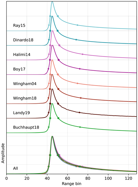
Figure 4 shows the waveforms calculated with all the delay-Doppler models for the Sentinel-3 Ku-band altimeter parameters for a Gaussian surface with a RMS height of 40 cm, without any volume underneath, the satellite perfectly at nadir with a circular antenna, no apodisation and the delay window widening of 2 (i.e. 256 gates are used before slant range correction). These simplified conditions are chosen to use only the common capabilities across all DDM models. For the models working with a deterministic DEM as input (Boy17, Landy19), independent samples of the Gaussian distribution were drawn for every 10 m×10 m cell in the footprint, thus allowing comparable behavior to the other statistics-based models. The waveforms are presented normalized to 1 at their maximum to facilitate intercomparison. The simulated waveforms have a typical shape of UF-SAR altimeter waveform on a flat surface (Raney, 1998; Aublanc et al., 2018) with a sharp rise (leading edge) and quasi-exponential decrease (trailing edge). This decrease is quicker than in LRM waveforms (Larue et al., 2021) because the surface area effectively contributing to each time gate (Fig. 1) is decreasing with time instead of being constant for the LRM as explained in Raney (1998). All the waveforms peak within the same range (bin 44.8–45.2), with the surface theoretically at gate 44 for Sentinel-3, as prescribed in the sensor's parameters in SMRT.

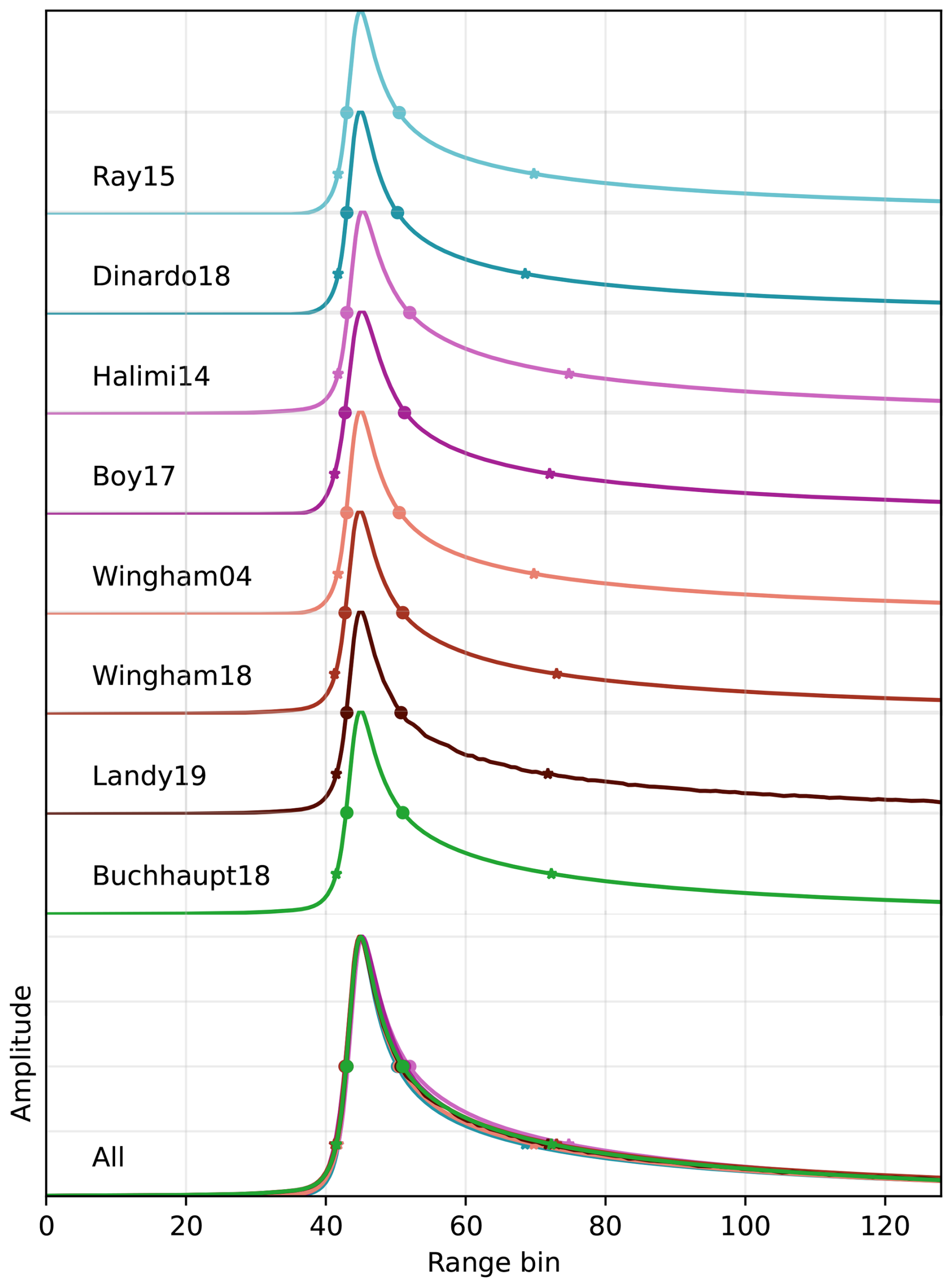
Figure 4 Waveforms computed by the 8 delay-Doppler map models implemented in SMRT for a surface with a large scale roughness σ_surf=40 cm (no snowpack). The sensor is Sentinel-3 at Ku-band. Markers are added at mid-height to help visualize the width of the peaks.

The waveforms are very close, but there are small observable differences when overlapping all the waveforms in a single graph (Fig. 5). The initial rise at the level of 5 % of the maximum is slightly earlier for Wingham18, Buchhaupt18, Landy19, Halimi14 than follows Wingham04 and Boy17 and finally Ray15 and Dinardo18 (Fig. 5a). The trailing edge at 20 % is earlier with Dinardo18 and Ray15, then Wingham04 followed by a group with Wingham18, Buchhaupt18 and Landy19, and finally Halimi14. These differences are likely due to a combination of theoretical and numerical approximations and the specificities of our implementation. As an example, the difference between Ray15 and Dinardo18 (e.g. the trailing edge is slightly later in Ray15) are likely numerical since the two models are in principle equivalent up to the final integration, which is performed numerically for the former and analytically for the latter. For Halimi14, we noticed that this model specifically requires a significant oversampling factor along the Doppler dimension (64 by default, vs. 4 for other models) to produce the same waveforms as the other models. This is due to the simplified integration over delay-Doppler cells, as exposed in their Eqs. (13)–(14) and the text around. This simplification is compensated here by oversampling.

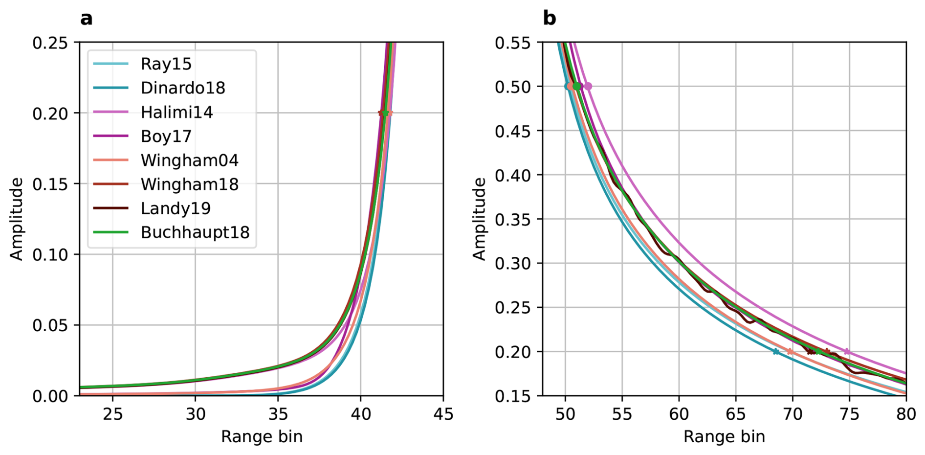
Figure 5 Zoom on the earliest echoes in the leading-edge (a) and in the middle of the trailing edge (b) in the same conditions as Fig. 4.

This comparison of the DDMs shows general agreement among the eight models, and the small differences observed are likely to be nonsignificant in most applications. However, the conditions of this comparison were chosen to allow a fair comparison. Each application should first review the approximations made by each model (e.g. Gaussian antenna pattern, statistical representation of the surface, Gaussian approximation of the PTRs, etc.) to decide which model or group of models is most suited. For instance, if the terrain slope is critical or the antenna is elliptical, not all the models are suitable.

5.2 Comparison with other altimetric models

To further verify our implementation, Fig. 6 compares Landy19 implementation in SMRT with the original Matlab model available as open source (Landy, 2022). The medium is a slightly rough surface at the radar scale (2 cm in RMS height and 7 cm in correlation length) and has a large scale roughness of 40 cm, with no slope and no underlying volume. For a fair comparison, SMRT was run with an oversampling time of 1, while the default is 4, and the original model used the geometrical optics approximation, whereas its default is I2EM (Landy et al., 2019). We normalized the backscatter to its maximum for comparison. The results show high consistency between the two models, with the difference not exceeding ±1 %. We note a smooth rise before the leading edge, possibly due to difference in the convolution of the PTR (as no echo is coming earlier than the surface echo, only the PTR influences the first gates), and a noise component all along the trailing edge, likely to the resolution of the grid (5 m in both simulations) and rounding errors. It is worth noting that when using a time oversampling of 4 in SMRT (results not shown), we observed a much larger difference, up to +14 %, due to a slightly earlier peak in SMRT, which could be incorrectly interpreted as a difference of surface elevation. Such results suggest to always compare simulations with the same oversampling and more generally call for careful consideration of the selection options when conducting precise comparisons or sensitivity analyses.

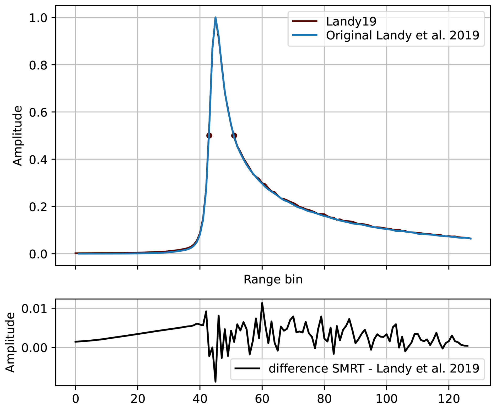
Figure 6 Waveforms computed by SMRT with the Landy19 DDM module and the original Matlab code (Landy et al., 2019). The medium is a surface only, with moderate radar-scale roughness (2 cm in RMS height and 7 cm in correlation length) and a large scale roughness of 40 cm, without slope. The sensor is Sentinel-3 (Ku-band).

A second comparison is performed to verify that pseudo-LRM waveforms calculated with DDM models is consistent with the output of the LRM module previously developed in SMRT (Larue et al., 2021). To simulate such pseudo-LRM waveforms it is necessary to disable the slant range correction. This is possible with most models, either because this correction is an independent geometric transformation applied directly to the DDM in the last stage of the simulation (Wingham04, Halimi14, Boy17), or because it appears as an explicit term in the equations, easy to disable (Wingham18, Buchhaupt18, Landy19). To our understanding, this is not possible with Ray15 and Dinardo18 because the correction is deeply embedded in their analytical derivation.

Figures 7a and b illustrate the DDM and waveform before and after slant range correction for Buchhaupt18 and Wingham18. The DDM without slant range correction show a typical parabolic shape (Halimi et al., 2014) explained by the fact that the distance from the satellite to reach the surface at a given look angle (i.e. Doppler bin) is increasingly further as the look angle increases, as illustrated in Fig. 1a. By summing this non-corrected DDM along the Doppler-frequency dimension yields the pseudo-LRM waveform (Fig. 7c) featuring a slowly-increasing leading edge and a decreasing trailing edge. In contrast, Fig. 7b shows the benefit of the slant range correction on the focusing of these high look angle echoes closer to the first echo (located at the nominal 44) and as a consequence, the resulting more peaked and narrower waveform.

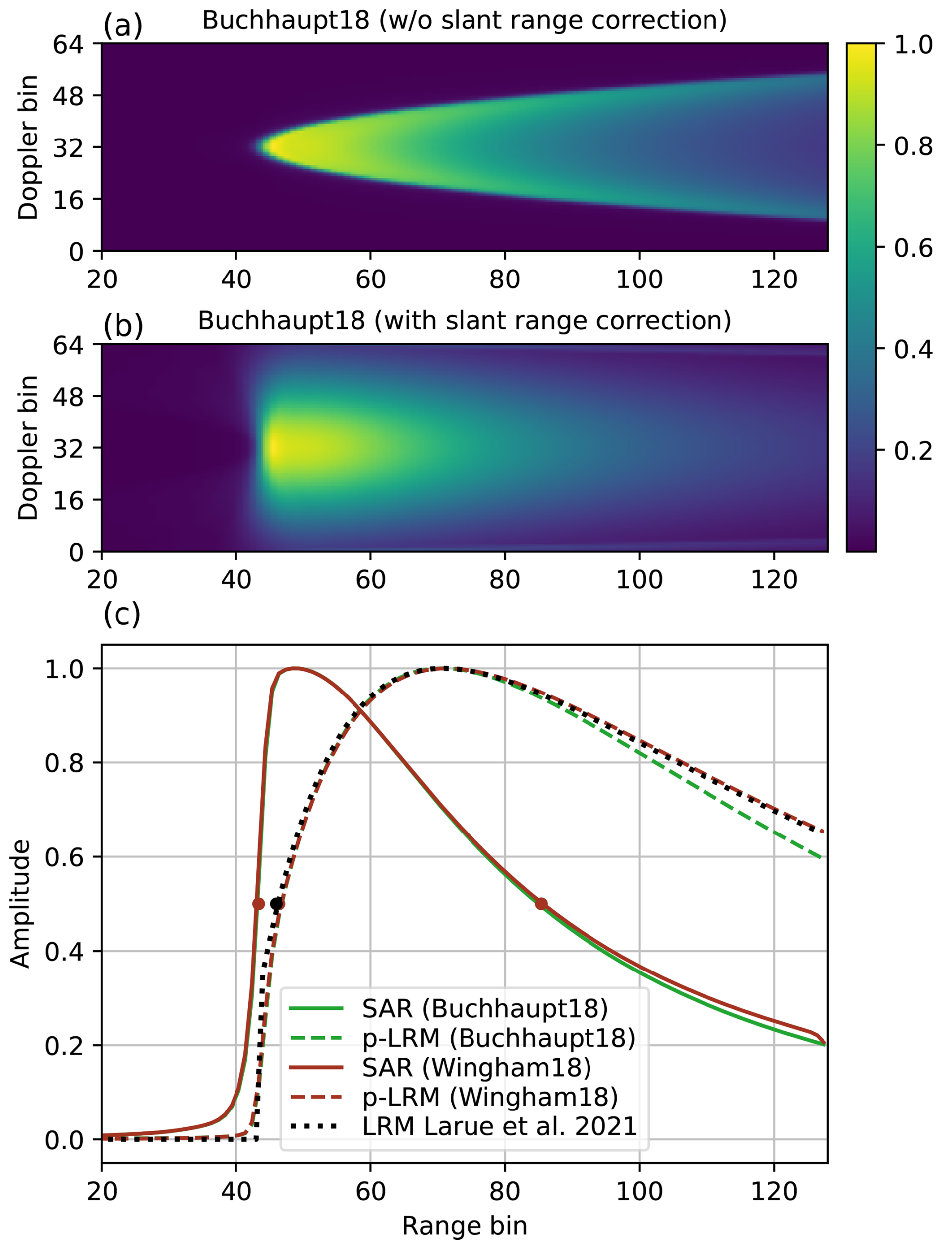
Figure 7 Delay-Doppler maps computed before and after slant range correction for Sentinel-3 with Buchhaupt18 and waveforms computed with three models: two SAR models developed in this study (Wingham18 and Buchhaupt18) before and after slant range correction and the original LRM model after Larue et al. (2021). The snowpack has a rough surface (RMS height of 2 cm, correlation length of 7 cm and large scale roughness of 40 cm) and is infinitely deep and homogeneous (density of 350 kg m⁻³ and microwave grain size of 0.2 mm, corresponding to an extinction coefficient of 0.10 m⁻¹).

Figure 7c compares these pseudo-LRM waveforms with the true-LRM calculation from the LRM module in SMRT (Larue et al., 2021) based on Brown (1977). The simulated snowpack is homogeneous and infinitely deep with a rough surface. This comparison with the original, independent LRM module shows near-perfect agreement with Wingham18. This provides a validation of our implementation, as both the LRM and SAR modules are completely independent. The agreement with Buchhaupt18 is also excellent in the leading edge, but degrades progressively in the trailing edge. Despite starting from the same principles as Wingham18, the elaborate Fourier transform approach may introduce small numerical errors.

5.3 Delay window widening

The comparison in previous Sect. 5.1 and 5.2 were conducted assuming that the time window recorded by the sensor extends well beyond the 128 gates. This choice was motivated by the need to achieve a fair comparison between all models since some are unable to account for the limited window of real sensors. However, for a comparison with real observations, when the surface is sufficiently rough, it is crucial to account for this detail as highlighted in Fig. 8. The figure shows the delay-Doppler map before and after slant range correction when considering either 128 gates (real case of Sentinel-3) or 256 gates (ideal case) and the resulting waveforms in both cases.

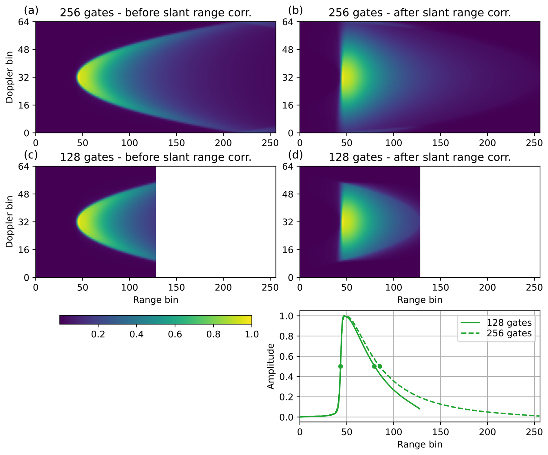
Figure 8 Delay-Doppler maps computed before and after slant range correction and waveforms for Sentinel-3 when using 128 or 256 gates. The DDM model is Buchhaupt18 and the snowpack has a rough surface at the radar scale (RMS height of 2 cm, correlation length of 7 cm and large scale roughness of 40 cm) and is infinitely deep and homogeneous (density of 350 kg m⁻³ and microwave grain size of 0.2 mm).

The simulation with 128 gates (Fig. 8b) shows that no signal is recorded at the highest positive and negative Doppler frequencies (bins <10 and bins >54) before the slant range correction because the echoes are coming beyond the 128th gate. Once the slant range correction (Fig. 8d) is applied, the signal is non-null only in a parabolic-shaped area. Comparing with the ideal focused DDM (Fig. 8c) gives an idea of the area of the DDM with missing power in the real case (Fig. 8d). Once summed along the Doppler dimension to obtain the waveform, and after normalization to the maximum, the impact on the waveforms is mainly visible on their trailing edge. The 128-gate simulations miss some power from the longest delays. This difference obviously increases at larger gate numbers, where more power is missing compared to the ideal simulations.

This change in waveform shape is significant and should be considered when comparing with observations, especially if the first echo occurs after the expected nominal gate (44 by default for Sentinel-3). In fact, the missing power strongly increases as the gate of the first echo arrival shifts to the end of the recording window.

In SMRT, it is possible to control the delay window widening factor for all but Ray15 and Dinardo18 models. The default factor is 1 (no widening), suitable for a comparison with observations, while 2 is usually sufficient to record all echoes, as shown in Fig. 8. All simulations in the previous sections use this value of 2. The user must be aware that, to achieve a realistic, limited window (no widening), a trick has been implemented in the models using an analytical slant-range correction (Wingham18, Buchhaupt18, and Landy19). In this case, the analytical correction present in the original studies is disabled and replaced by the numerical method used in other models (Wingham04, Halimi14, Boy17). This trick is automatically enabled for a widening of 1 (or less) while the original analytical correction is applied for larger widening.

5.4 Simulations with separated contributions

In addition to returning the total DDM, the SAR module can optionally return the contributions from each layer and each interface, and separate coherent reflections from incoherent ones. Figure 9 illustrates this feature for a snowpack with a rough surface (3 cm RMS height) and a smooth crust (0.5 cm RMS height, 450 kg m⁻³ and microwave grain size of 0.3 mm) buried at 2 m depth. The layer above the crust is composed of fresh snow (300 kg m⁻³ and microwave grain size of 0.1 mm) and the semi-infinite layer below of older snow (350 kg m⁻³ and microwave grain size of 0.2 mm).

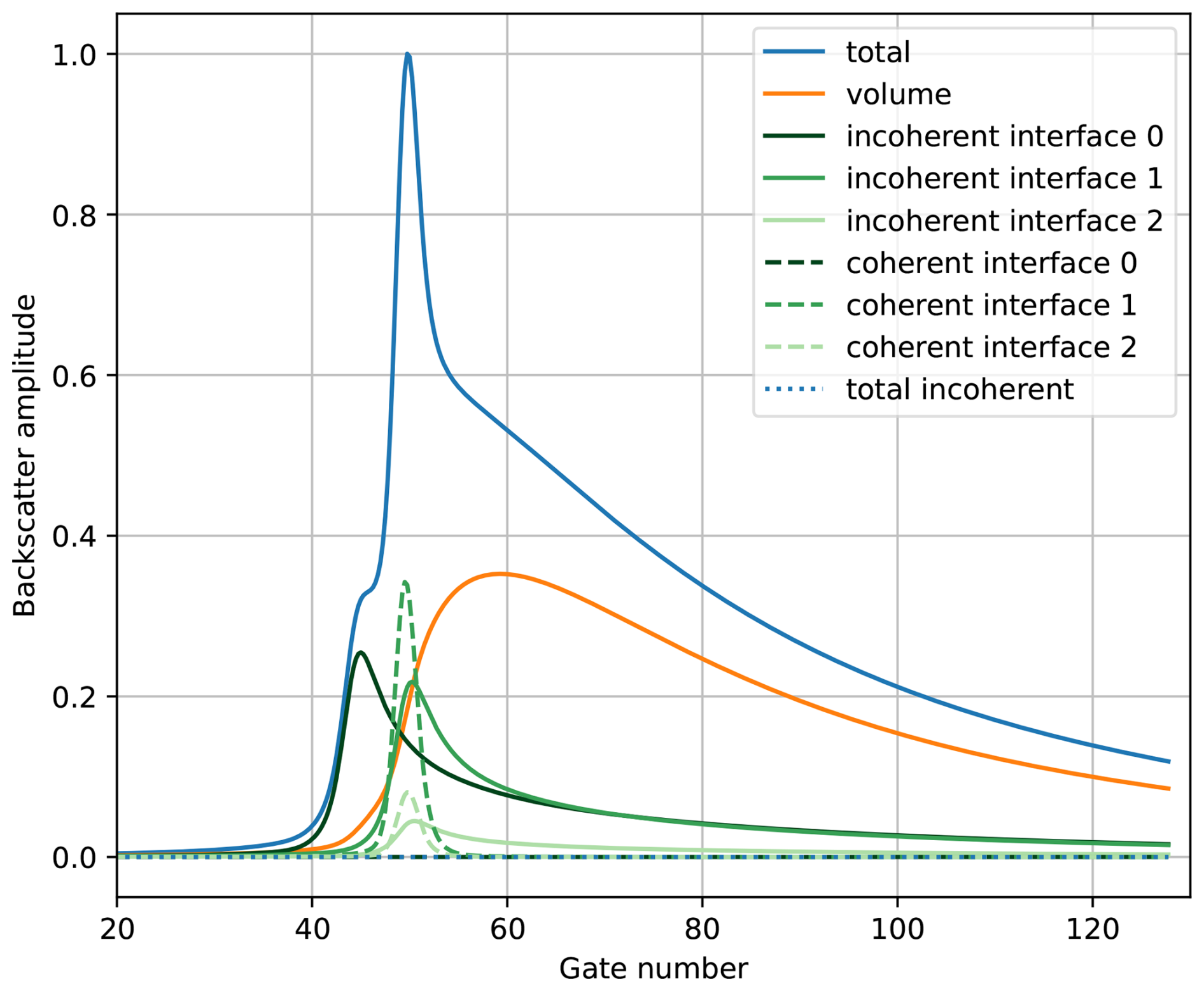
Figure 9 Waveform calculated using Buchhaupt18, with the respective incoherent and coherent contributions from the volume and the interfaces. The sensor is Sentinel-3 in Ku-band. The snowpack surface is rough (interface 0, with RMS height of 3 cm) and a 10 cm thick melt crust is at 2 m in the snowpack (interface 1 and 2, top and bottom of the crust).

The simulation considers a specific snowpack to illustrate the signal components. Although such crust layers exist, the particular shape of the simulated waveform may not be observed in reality due to speckle noise and the non-uniformity of the snowpack over the kilometre-wide footprint. The volume (orange) has the largest contribution but is delayed relative to the surface echo (interface 0, dark green). The surface has a strong incoherent contribution and virtually no coherent contribution, due to the high RMS height of 3 cm. The top and bottom sides of the crust layer (interfaces 1 and 2, respectively) have a moderate incoherent contribution (light green solid curves) and a coherent peak around gate 49 (light green dashed curve). This coherent peak is due to the layer's smoothness. It is worth noting that this idealized simulation assumes a sensor pointing precisely perpendicular to the crust layer. With a satellite pitch angle as small as 0.3°, the coherent contribution immediately vanishes (not shown).

5.5 Validation in Antarctica

5.5.1 Simulations with in-situ measurements

Figure 10 shows the Sentinel-3 SRAL simulations at 12 Antarctic sites using in-situ measurements only as inputs of the simulations. No simulations were run at the 6 other sites due to missing MSS measurements. The sites are sorted by latitude, from South (on the high Plateau) to North (towards the coast). We selected the Buchhaupt18 model here, for its computational efficiency.

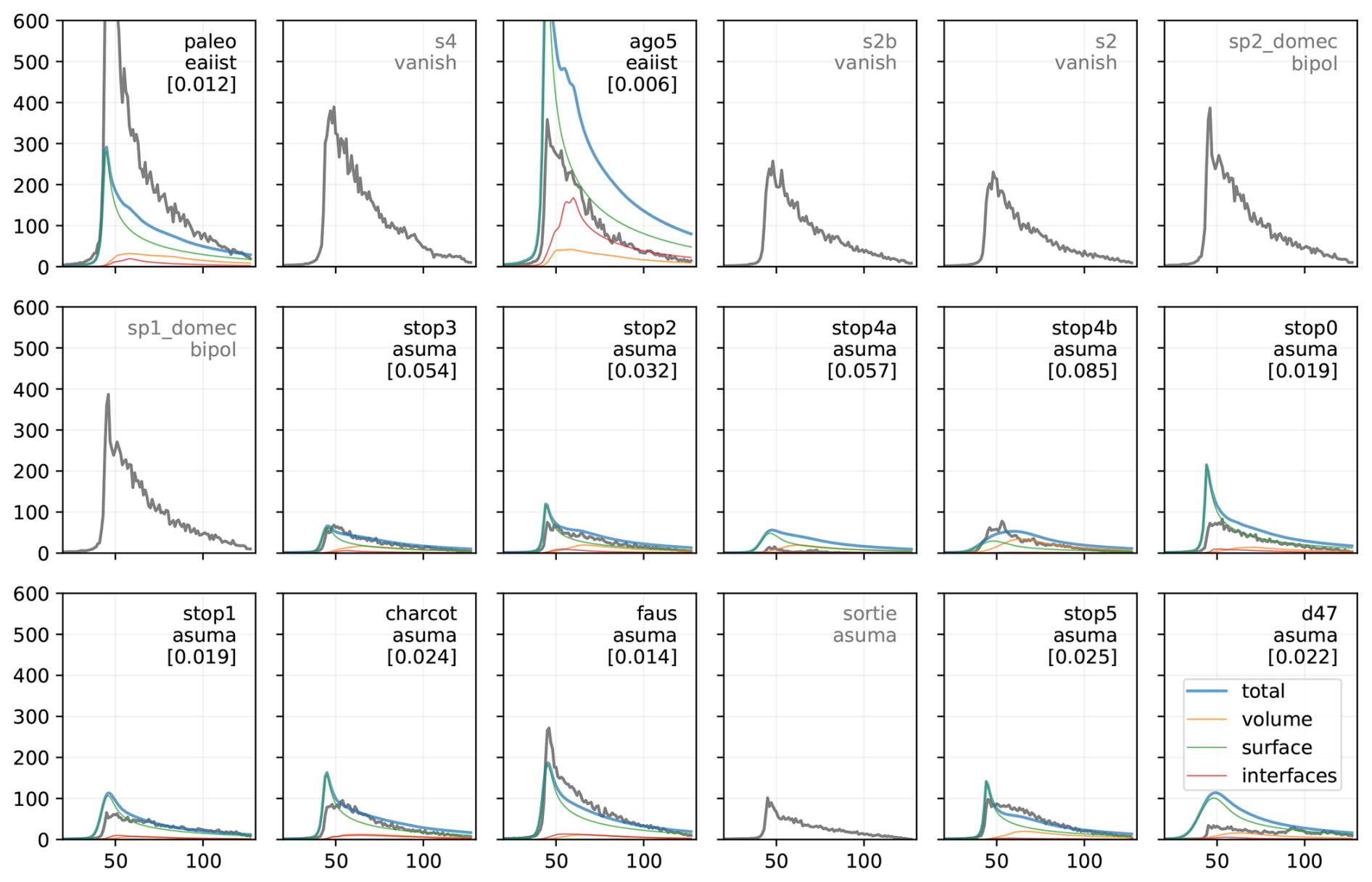
Figure 10 Observed and simulated waveforms at 12 Antarctic sites (from South to North) for Sentinel-3 SRAL, using Buchhaupt18. The simulations use in-situ measurements exclusively; only a global scaling factor is applied to account for the altimeter's missing absolute calibration. The y-axis units are arbitrary. The value in bracket is the measured mean square slope (MSS).

The amplitude of the observed waveforms (gray) is generally higher at Dome C and further South, while it is lower in the ASUMA area, except at the faus and stop0 sites, which exhibit intermediate behaviour. Overall, the simulations align with this latitudinal gradient, which is consistent with the findings of Larue et al. (2021) for the LRM mode.

The results are primarily driven by radar-scale roughness. The surface is indeed the main contributor to the simulated waveforms (green), followed by the volume (orange) and the internal interfaces (red). Over the ice-sheet, radar-scale roughness variations are mainly related to wind strength, which is modulated by the topography in the katabatic regime prevailing over Antarctica (Van den Broeke and Lipzig, 2003; Poizat et al., 2024). The interior regions of the East Antarctic Plateau, especially near the domes, are flatter and experience lower wind speeds, resulting in smoother surfaces than the outer regions (such as the ASUMA area).

The contributions of the volume and internal interfaces are weak but not negligible at any site. These contributions primarily control the trailing edge in the simulations, since the echo arrives later than the surface. The volume contribution is slightly larger at the southern sites, peaking earlier (at gate 58), whereas the opposite is usually observed at the ASUMA sites (peak at gate 65). This is explained by the presence of coarser snow grains on the Plateau, due to the lower accumulation, a well-known characteristic that also significantly affects passive microwave signals (Brucker et al., 2010). Larger grains scatter more, leading to higher backscatter and increased extinction, resulting in shallower wave penetration.

Beyond the amplitude, the shape of the waveforms shows notable variations across the sites. Some waveforms exhibit a sharp peak near the maximum (stop2, stop0, charcot, stop5), which can be attributed to a large surface contribution relative to the volume and internal interfaces. In contrast, the peaks are more rounded at sites like stop4a, stop4b, and d47, where the large scale roughness is relatively extreme, as shown by the REMA standard deviations >1.7 m in Table 5. Like the simulations, the set of observed waveforms shows evidence for scenarios when the surface echo dominates (sharper first maximum, e.g. sp1_domec, sp2_domec, sortie, faus) and scenarios when the volume echo dominates (rounded, e.g. stop5), but the relative dominance for a specific site is not always predicted in the simulations.

Aside from the clear south-to-north gradient evident in both the simulated and measured amplitudes, it remains difficult to determine whether the model performs well. The need to adjust the global scaling factor, the uncertainties in the measurements (particularly the radar-scale surface roughness) and the observational noise all complicate the comparison. It is clear, however, that the radar-scale surface roughness parameters are key, having a first-order impact on the modelled waveform amplitudes and controlling the relative contributions of the surface and interface vs volume echoes.

5.5.2 Simulations with optimized radar-scale roughness

To make use of the sites with missing radar-scale roughness measurements and explore the uncertainty related to surface roughness, we optimized the surface MSS values at each site to match the observed and simulated backscatter. We assume the internal interfaces have the same roughness as the surface. The new simulations shown in Fig. 11 are greatly improved and closely match the observations at most sites, highlighting the strong control of radar-scale surface roughness on the altimetric signal.

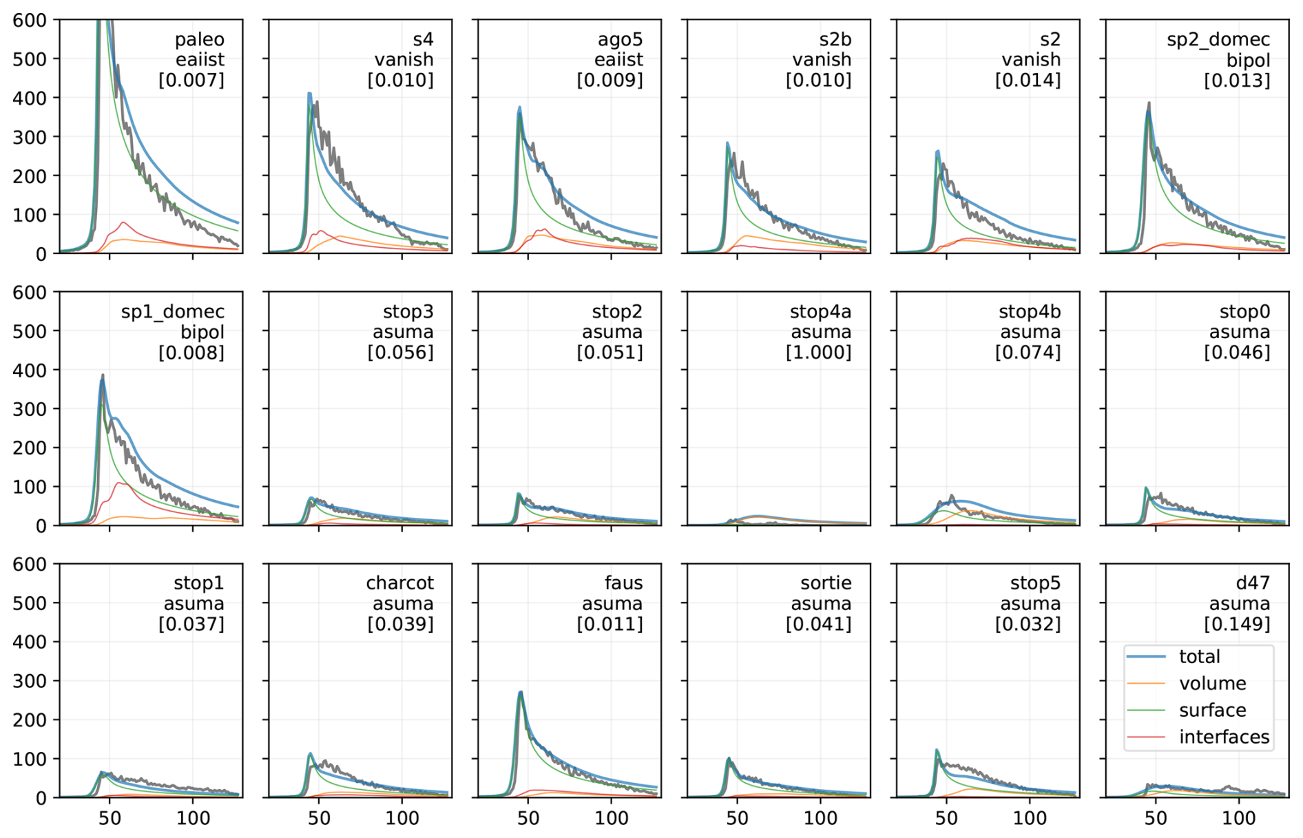
Figure 11 Same as Fig. 10 except the mean square slope (MSS) of the surface and interfaces is optimized for each site to match the observations. The value in brackets is the optimized mean square slope (MSS).

In general, our optimization procedure tends to prioritize matching the observed and simulated leading edge and the waveform maximum for two reasons: first, because the definition of ICE-1 amplitude gives more weight to the higher waveform values with the exponent 4 in Eq. (7), and second because only the surface echo governs the leading edge, while the volume and internal interface contributions arrive later. The good agreement found between observed and simulated leading edges is therefore likely due to the optimization process. However, accurate simulations of the trailing edge require the model to correctly estimate the volume and interface contributions relative to the surface contribution. There is evidence of correctly modelled backscatter contributions at several ASUMA sites (e.g. stop2, stop3, faus, sortie), where the volume bump precisely balances the rapid decline of the surface echo, leading to excellent agreement. In the passive microwave study by Picard et al. (2022b), which used the same field data, the ASUMA sites also showed the best alignment at 10 and 19 GHz, confirming the quality of the SMRT volume estimation at these locations. There is also evidence at e.g. sp1_domec and ago5, that internal interfaces make strong contributions to the trailing edge of the observed waveforms, with step-like shapes.

Simulations at stop0, Charcot, and stop5 exhibit a sharp leading edge and a rapid initial decline at the trailing edge, followed by a more gentle decrease, suggesting that topographic variations are larger than those estimated from the REMA DEM. It might also be due to the neglected slope. Alternatively, the volume might be slightly underestimated or delayed. The worst results were observed at stop4a and stop4b, which correspond to the roughest terrain among the test sites with extremely high heterogeneity (σ_surf in Table 5). These results from the rough northern sites demonstrate the limits of using a statistical representation of topography for ice sheets. Instead, it is recommended to use real DEM and models such as Boy17, Landy19 or Aublanc et al. (2025a).

6 Discussion

6.1 Limitation of the comparison

To check our implementations, we performed several comparisons: first between the eight implemented DDM models; then between Landy19 and the original code in Landy et al. (2019); and, last, between Buchhaupt18 and Wingham18 in pseudo-LRM mode with respect to the original LRM implementation in Larue et al. (2021). The two former considered a surface only, and the latter also included a volume. In general, these comparisons show good agreement, and the residual differences were attributed to numerical errors (particularly evident in Landy19) or to formulation and implementation details (between Ray15 and Dinardo18). However, to achieve such an agreement, it has been necessary to devise a simple medium configuration (statistical representation of the terrain with a Gaussian approximation, no slope, circular antenna) and to carefully adjust the model settings (widening factor =2). While this approach fits with our goal of cross-validation, these settings are not the default in SMRT (widening factor =1 except in Ray15 and Dinardo18), and are usually not the same as in the original studies (e.g. the topography representation, the Gaussian approximation of the terrain distribution and of the PTR). For future use of this SAR Altimetry module, it is recommended to (i) refer to the documentation and source code for the default settings and the specific capabilities of each DDM model (e.g. Landy19 using the accelerated sinc² transform is incompatible with the Hamming window which the Matlab code can account for), (ii) prefer the most recent models (post 2017) that account for the terrain slope and antenna asymmetry, (iii) perform an initial cross-comparison with as many DDM models as possible in the conditions relevant for the application (for instance for using a real DEM, both Boy17 and Landy19 are suitable, and comparing Wingham18 and Buchhaupt18 may reveal numerical issues due to the Fourier transform), and (iv) carefully check and adapt the altimeter parameters (e.g. PRF and altitude) as well as understand the adequacy of the selected DDM model and the specific L1 ground processing settings (e.g. oversampling in range, selection of the beams in the stack, etc).

6.2 Limitations of the validation

In the comparison in Antarctica, the SMRT model was able to predict the waveform shape and the spatial gradient in waveform amplitude using only in-situ measurements, and performed better when optimizing the radar-scale surface roughness. The shape is primarily controlled by the delay-Doppler map model, and secondly by the correct balance between the surface and volume (and interfaces) contributions. Despite the significant improvement brought by the surface roughness optimization, the results show irreconcilable discrepancies, as in stops 4a, 4b, 1, and 5. Part of this may be attributed to the following limitations of our approach.

The in-situ measurements are taken at a single point on a single date and used to represent a wide footprint across distant observations in time. The representativeness is a common issue in remote sensing and modelling, but one should mention that the skills of SMRT observed in the passive microwave with resolution >25 km (Picard et al., 2022b) are indicative that the large scale variations in Antarctic snow and surface properties are more important than the intra-footprint variability, though it could not be excluded. The Antarctic snowpack is also very stable far from the coasts. The most volatile variables are certainly the radar-scale surface roughness, grain size and density, with a dynamics related to storms and snowfall events (Amory et al., 2016; Studinger et al., 2020; Stefanini et al., 2024). The exploration of the temporal dimension is left to future work.

The second main limitation of our approach is to consider a Gaussian topography and neglect the slope. It is now well demonstrated that the exact topography within the footprint has a considerable control on the waveform shape (Aublanc et al., 2025a). It is interesting to note that Aublanc et al. (2025a) obtained excellent results in terms of waveform shape while only considering the surface. However, neglecting the volume and the penetration of the wave is likely to bias the retrieved elevation. To explore this aspect further, the Boy17 and Landy19 delay-Doppler models are suitable, as a real DEM can be prescribed. This has not been tested and is also left to further work.

6.3 Limitations of the new SAR module and perspectives

The newly implemented module and its delay-Doppler models have several limitations that may affect results in the present study and future investigations.

The medium is assumed homogeneous over the entire footprint, which typically extends to a dozen of kilometres. This limitation owes to the current implementation, and although the studies reviewed in Sect. 2 do not account for heterogeneity, the models using an explicit spatial grid are easily amendable (namely Landy19 and Boy17) as long as 3D effects remain negligible (i.e. no lateral wave propagation across different media). The main cost is to repeat the computation of the scattering properties of each medium within the footprint, which is moderate compared to the computation of the delay-Doppler map itself using these most numerically intensive models. On the ice-sheets, the benefit would be to account for the spatial variability, but this would require a realistic set of in-situ measurements. However, the main gain would be for simulating strongly heterogeneous targets like sea ice and frozen lakes in the presence of leads, as newly-forming ice in leads acts as a strong coherent radar reflector and thus shows a contrasted response to the sea or lake ice floes (Bocquet et al., 2023).

Another limitation arises from the single-scattering calculation of the echo: the wave is reflected by the surface, an interface, or the volume only once, while interactions involving double bounce and higher-order scattering are neglected. These interactions are susceptible to increasing late echoes, because of the longer travel, with an impact on the trailing edge and possibly double peaks. Overcoming this limitation is not straightforward and would practically require using intensive ray tracing techniques to compute interactions while recording time of flight (Winiwarter et al., 2022). In general, multiple scattering in the volume is likely to affect the highest frequencies, i.e. the Ka-band altimeters, although the extinction is also high when multiple scattering exists, limiting the distance between two interactions, and so the delay. Reflection in layered media at low frequency and low temperature, where absorption is reduced, may also be subject to multiple scattering and relatively long distances between reflections. A first practical way to assess the amount of volume multiple scattering consists in computing the approximate fraction due to higher order scattering $\stackrel{\mathrm{̃}}{\mathit{\omega }}/(\mathrm{1}-\stackrel{\mathrm{̃}}{\mathit{\omega }})$), where $\stackrel{\mathrm{̃}}{\mathit{\omega }}$ is the single scattering albedo. The typical distance between two interactions is estimated by the inverse of the extinction coefficient (i.e. the e-folding depth). Both are outputs of SMRT simulation for each layer. For instance, the average single scattering albedo over the top meter of the snowpack reaches 0.39 at ago5 and s2b for Sentinel-3 in Ku-band, with an e-folding depth of 22 m (about 50 range gates). This value rises to 0.76 at 35.75 GHz (Ka-band), the frequency of the future Copernicus CRISTAL (Kern et al., 2020), indicating strong higher-order scattering in the volume. However, the e-folding depth is significantly reduced to 1 m (about 3 range gates). Another approach consists of comparing the backscattering coefficient simulated using the first-order iterative solver (single scattering only) and the DORT solver, which accounts for all scattering orders (Picard et al., 2018). This approach also accounts for the between-interface multiple scattering. At ago5, we found a difference of 2 dB in Ku-band (63 % of the amplitude is due to single scattering), and 4 dB in Ka-band (43 % is due to single scattering). The comparison between observed and simulated waveforms may also bear the imprint of missing multiple scattering, with the simulated trailing edge underestimated and a secondary peak appearing in the observations.

Another point of attention is the approximate nature of the delay-Doppler models and the numerical inaccuracies arising from implementation details, as illustrated in the results (Sect. 5). These models simulate the effect of the UF-SAR processing but are not simulators of the full complexity of modern SAR processing. In particular, except Landy19 they do not account for stacking multiple acquisitions as the AMPLI model does (Aublanc et al., 2025a). The current implementation also misses FF-SAR and SARIn processing, for applications to Copernicus Sentinel 6 (Donlon et al., 2021) and CRISTAL over sea ice (Kern et al., 2020). However, it is suitable to extension, simply by implementing a new delay-Doppler map model for these processing (e.g. Egido and Smith, 2017; Hernández-Burgos et al., 2024). More complex would be the adaptation to airborne altimeters, because the assumption of small near nadir angles is used in the main nadir_sar_altimetry module as well as in the DDMs.

7 Conclusions

The SMRT version 1.7 now includes a comprehensive UF-SAR altimetric module to compute delay-Doppler maps and waveforms for cryospheric environments, enabling satellites such as CryoSat-2 and Sentinel-3. The main skill of SMRT is the fine description of a wide variety of cold environments and the precise calculation of scattering and absorption in snow and ice. With the former Low Resolution Mode (LRM) module and the present implementation of eight different delay-Doppler map models from the literature, published from 2004 to 2019, the possibility of using SMRT for altimetric signal investigation is high and new. Furthermore, the implementation of new delay-Doppler models, for instance for SARIn and fully-focused processing for application to CRISTAL and Copernicus Sentinel-6, is also greatly facilitated. As the entire SMRT framework is now established and well tested by an increasing number of researchers, only the essential altimetric signal equations need to be implemented and validated to develop a new operational module.

The present study assessed the new module's ability to simulate the Antarctic ice-sheet UF-SAR altimetric signal, achieving reasonable agreement. However, much further work is needed to explore the vast number of parameters in the altimetric modules and the functionalities implemented but still unexplored, as well as to test the ability of the models to simulate other environments such as sea-ice, lake-ice and seasonal snow. Results from the Antarctic ice sheet at least confirmed the importance of radar-scale surface roughness in controlling the weighting between backscatter contributions from the surface and those from snow volume. Beyond the ice sheets, an important application of this new version of SMRT is the investigation of the penetration bias and the dominant scattering horizon for sea ice and frozen lakes to improve retracking for CryoSat-2 and Sentinel-3.