CMIP6 data usage: lessons learned from more than 200 million downloads

Earth system simulations from the Coupled Model Intercomparison Project (CMIP) are considered the gold standard in terms of representation of the Earth's climate system, its past and present states, and possible future evolution. As CMIP moves into its seventh phase, the increasing complexity of Earth system models (ESMs) means that there is a greater need for infrastructure resources to store, distribute and utilize CMIP simulations. Statistics on the usage of data during CMIP6 has the potential of offering guidance to prepare for CMIP7. Here, we analyse the downloads of CMIP6 data and propose recommendations for optimizing the production and accessibility of future CMIP data. Our analysis focuses on CMIP6 data downloads statistics from the Earth System Grid Federation (ESGF), the main database of CMIP and other ESMs simulation data. We perform an analysis of CMIP6 ESGF data downloads statistics, with a focus on variables, experiments, individual thematic Model Intercomparison Projects (MIPs), sources and institutions, and related geographical download trends. We further complement the ESGF analysis with statistics on access from other sources hosting CMIP6 data, including some curated by community portals (Pangeo) through commercial clouds (Google Cloud and Amazon Web Services) and by climate services (Copernicus Climate Change Service). We conclude with recommendations for centres involved in the production and distribution of data to optimise resources based on download statistics, to perform stronger quality checks, and to implement improved approaches to track usage.

1 Introduction

As the complexity and number of climate models increased during the last century, standards for the comparison of models became necessary (Meehl, 1995; Meehl et al., 1997). These developments culminated in the first model intercomparison initiative, the Atmospheric Model Intercomparison Project (AMIP I) in 1990 (Gates et al., 1999). A similar initiative for coupled models followed in 1995 and thus the Coupled Model Intercomparison Project (CMIP) was born (Meehl, 1995; Meehl et al., 2005). These projects provide standard protocols for climate model simulations to facilitate a straightforward comparison of outputs from an increasing number of models. Over time, more and more model intercomparison projects (MIPs) were created. CMIP6 alone endorsed 21 MIPs that cover specialised subject areas with more than 300 different experiments (for CMIP6-endorsed MIPs see for instance Eyring et al., 2016). Additionally, there are a small number of common experiments, the Diagnostics, Evaluation and Characterization of Klima (DECK), historical simulations, as well as shared infrastructure and standards (Eyring et al., 2016).

The CMIP community has gone to great lengths to make model output interoperable and as accessible and understandable as possible in an unprecedented cooperation effort between modelling centres from around the world. The successes of this cooperation are remarkable considering the diversity of scientific foci at modelling centres, as well as physical assumptions and parameterizations used in models and the grid design and chosen resolutions. To bring the different approaches together, CMIP established controlled vocabularies (CVs) with standardized descriptors for categorizing and sorting CMIP simulation data (Eyring et al., 2016). Additionally, the CMIP6 data request team (Juckes et al., 2015, 2020) provided information on the variables requested by individual MIPs. To top it off, the Earth System Grid Federation (ESGF), as a collaboration of climate data centres, makes the simulation data available through a shared data distribution infrastructure. Many more initiatives emerged and as a result a wealth of information and tools related to CMIP are accessible through the community (https://wcrp-cmip.org, last access: 15 November 2025).

At the same time, the computational demand for running the models, as well as the data volumes produced and stored have increased sharply with successive CMIP cycles (Durack et al., 2025). Submission to CMIP6 closed in 2025 with more than 16 PB of distinct datasets published according to the ESGF Data Statistics service (https://esgf-ui.cmcc.it/esgf-dashboard-u, last access: 15 November 2025). This demand on computational infrastructure has a significant carbon footprint. For example, Acosta et al. (2024) estimate that the 14 European institutions of the IS-ENES3 consortium produced almost 1700 t of CO₂ equivalent when running their CMIP experiments by the end of 2020, corresponding roughly to the annual emissions of about 200 average US citizens (Voosen, 2024).

Moving into CMIP phase 7, an efficient allocation of resources is vital considering the growing demand on the computational infrastructure, in particular with respect to storage. Here, statistics on the usage and downloads of data during the CMIP6 cycle can offer guidance. In this manuscript, we aim to analyse the usage of CMIP6 data and propose recommendations for optimizing the production and accessibility of it.

2 Data

CMIP6 data can be downloaded and accessed from different sources. The main and original source are the Earth System Grid Federation (ESGF) nodes (Sect. 2.1). As the most comprehensive statistics are available for ESGF downloads, their analysis forms the core of this manuscript. On top of this, there are CMIP6 data sources that are separated from the ESGF system. These provide only a subset of all CMIP6 data, but are still important for CMIP6 data users (Balaji et al., 2018). For example, a subset of CMIP6 data curated by the Pangeo open source community, coordinated by the Pangeo/ESGF Cloud Data Working Group (https://pangeo-data.github.io/pangeo-cmip6-cloud/, last access: 18 February 2026), can be found on commercial clouds in buckets¹ from Google Cloud and Amazon Web Services (AWS, Sect. 2.2). The Copernicus Climate Change Service (C3S) also provides direct downloads for a small subset of CMIP6 data, in collaboration with some European ESGF nodes (Sect. 2.3).

The CMIP6 survey further highlights the widespread use of national and shared resources, such as CAFE (China), DKRZ (Germany), DIAS (Japan), UKRI (UK), NCAR (USA), NCI (Australia), for data analysis by 38 % of survey respondents (O'Rourke, 2023). Shared resources include copies that have been downloaded from ESGF, as well as direct access to some ESGF data nodes themselves. Indeed, some ESGF node installations host original data from their institutions, as well as replicated data from other institutions. For example, in March 2023, DKRZ hosted 1500 TB of original data and 2400 TB of replicated data (Kindermann et al., 2023). This replication makes the network more resilient, enabling users to download data from multiple nodes. It further removes the necessity for some individual users and research groups to download large volumes of data. These replica sites allow the users at an institution remote access to the data but also, to have access to computing resources at the infrastructure hosting the data. Data usage through these and smaller institutional archives or servers is not recorded in any usage statistics and thus inaccessible for our analysis. Because of this, we expect we are missing a substantial part of data usage from users with access to these archives, especially in Europe where there are more ESGF data nodes with replicated data (e.g., DKRZ, CNRS-IPSL, UKRI).

2.1 ESGF

The ESGF nodes are the main archive for CMIP6 data. ESGF is a federation of government agencies, institutions, and companies that develop and maintain a huge decentralised platform for climate science data in a worldwide collaboration. The CMIP6 ESGF architecture is based on a system of autonomous and nodes distributed across different sites (North America, Europe, Asia and Australia). It hosts data from several projects, for the most part CMIP, including community MIPs and CORDEX, providing access to petabytes of climate model and other geophysical data. For CMIP6, more than 14.8 million datasets are available for a total of almost 28 PB of data, out of which about 7.6 million are distinct datasets and the remainder replicas (https://esgf-ui.cmcc.it/esgf-dashboard-ui/federated-view.html, last access: 15 November 2025).

To better understand the patterns of downloads from ESGF, the CMCC (Centro euro-Mediterraneo sui Cambiamenti Climatici) developed a system to monitor the nodes and log the downloads. Some of the statistics they gathered are publicly summarized and available through the ESGF Data Statistics service, covering downloads starting from January 2018 (https://esgf-ui.cmcc.it/esgf-dashboard-ui/cmip6.html, last access: 15 November 2025). The publicly available information includes download statistics on variables, experiments, sources (that is model version and configuration), institutions, as well as countries or regions from which a download originated, all of which we analyse in Sect. 4. For all statistics, the number of downloaded files and the downloaded file sizes in GB are recorded. The ESGF Data Statistics service includes data from only 19 nodes (including old nodes that are no longer operating). Hence, some data might be missing from nodes that are not tracked. There could also be some missing data due to technical issues in tracking some nodes (this happened to the CCCma node for instance during the period we analyse). In total, we use statistics up to 13 January 2025 covering 236 732 332 logged downloads and roughly 41 PB of data downloaded. CMCC has been monitoring these download statistics over time and in more detail than is available through the ESGF Data Statistics service, but unfortunately the database was inaccessible during the preparation of this manuscript due to a migration of the hosting infrastructure. For statistics on the amount of available data, we queried the ESGF index directly.

2.2 Commercial clouds

A subset of the CMIP6 data is also available on commercial clouds, in particular the Google Cloud and Amazon Web Services Simple Storage Service (AWS S3) commercial clouds, following collaborations between cloud providers, ESGF, the Pangeo open source community (via the Pangeo ESGF Cloud Data Working Group), and the LEAP project (Busecke and Stern, 2024). These are public and free to use, hosted under Amazon's Sustainability Data Initiative and Google's public datasets programmes, but without guarantees regarding longevity of the datasets. These caches of analysis-ready cloud-optimised (ARCO) data (Stern et al., 2022) have the key advantage that users can “lazy-load” data, working with it in object storage while only streaming the subset of data required for a given analysis. ARCO formats also take advantage of the high latency but high parallel throughput features of cloud object storage. Hosting data in the cloud also allows for data proximate computing (Ramamurthy, 2017), which avoids the need to download and store copies of large databases and thus has the potential to expand access to environmental data and empower communities that have historically been marginalized and lack local or shared computing resources (Gentemann et al., 2021). As such, we are not looking at download statistics as for ESGF, but rather access statistics.

For Google Clouds, no statistics were recorded. AWS provides services which enable tracking of access metrics for the CMIP6 data, which were kindly made available to us. We analysed AWS S3 data for the period from 16 February 2022 to 31 May 2023. Only a few daily statistics are available: the number of accessed files, the number of unique IPs and the data transferred in GB (only from June 2022 onwards).

2.3 Copernicus Climate Change Service (C3S)

The Copernicus Climate Change Service is hosted by the European Centre for Medium-Range Weather Forecasts (ECMWF). Their mission is to “support adaptation and mitigation policies of the European Union by providing consistent and authoritative information about climate change” (https://climate.copernicus.eu/about-us, last access: 15 November 2025). To do so, they provide a large number of climate datasets, including CMIP6 climate projections. The data is distributed through the climate data store (CDS; Buontempo et al., 2022). Users can download the data using the website or the CDS API. C3S provides only 43 monthly variables, 7 daily variables and 8 fixed variables from the historical experiment and 8 SSP scenarios through a collaboration with major European ESGF replica nodes (IPSL, DKRZ, CEDA). An interesting feature of the CDS interface is that it provides computing resources to subset the data geographically or by time. This subsetting functionality can be particularly useful for users who do not have access to large storage spaces or are only interested a specific region/time period.

C3S gathers statistics on the number of requests received and the number of users. Note that these are different statistics from the ones provided for ESGF (total size of downloads and number of downloads). The two sets of statistics do not represent the same type of user interaction with the platform and cantherefore not be directly compared. The downloads statistics used in the analysis were gathered from September 2024 to August 2025. A different system was used to gather statistics prior to this period, with more than 10 000 unique active users of CMIP6 data logged with the previous system. During the recent period, there were 3551 active users that downloaded 38 696 GB of data through 595 319 successful requests. Since the two systems do not use the same variable naming convention, we mapped C3S long names to the official CMIP6 CVs.

3 Download patterns in ESGF data

In this section, we analyse the usage of ESGF data, for which the most comprehensive statistics are available, with regards to different aspects. We look at the usage through the lens of downloads. This can only offer a limited and imperfect view of usage, as many other factors can influence the downloads statistics. Indeed, the size of a dataset will directly inform the size of downloads, giving larger datasets an outsized weight. On the other hand, users might also refrain from downloading large datasets due to resource constraints. The number of files in a download request also depend on the characteristics of the dataset, as well as modelling centres' choices for archiving. Factors influencing the downloads include, but are not limited to, time resolution, spatial resolution, number of vertical levels, ensemble size, time coverage, number of variables and experiment chosen by a modelling centre and publication of new versions. More details on the specific influences are discussed in each of the subsections.

3.1 Variables

CMIP6 variables are distributed at different frequencies from sub-hourly (subhrPt) to yearly (yr). Figure 1 shows the downloads for each of these frequencies. Daily and monthly are the more downloaded frequencies. Daily data is often the basis for widely-used climate indicators, such as the ETCCDDI indices (https://etccdi.pacificclimate.org, last access: 15 November 2025). Monthly data is often used for calculation of global quantities. High-frequency data are, by definition, much larger in volume which can hinder downloading (and subsequent analysis) by users. This may explain the low number of downloads for frequencies subhrPt and 1 h.

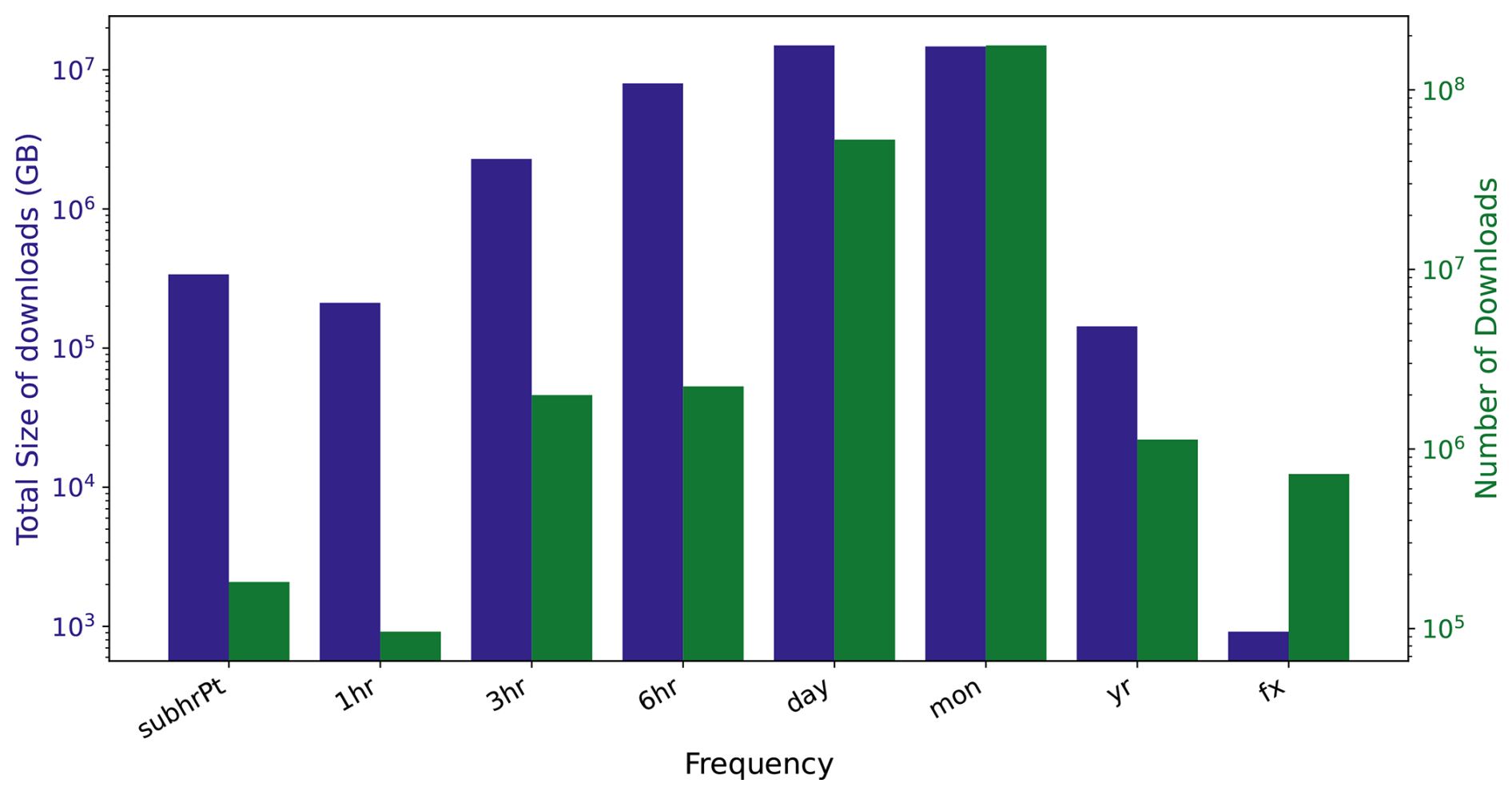
Figure 1 Total size in GB (blue) and number of downloaded files (green) for each frequency. The long names of the frequencies are available at https://github.com/WCRP-CMIP/CMIP6_CVs/blob/main/CMIP6_frequency.json (last access: 15 November 2025).

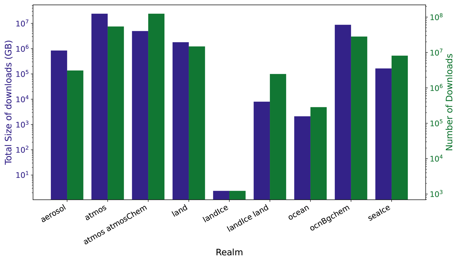
Variables are also split by realm (Fig. 2), with atmosphere dominating the downloads (if we sum the atmos and atmosChem categories). Mixing frequency and realm, we get tables, such as Amon for monthly variables in the atmosphere realm. In CMIP6, individual variables are defined by a base name and a table (e.g., ua_Amon)². In the CMIP6 controlled vocabulary, there are 43 accepted tables and 2062 accepted individual variables (see id and full names in Tables S1 and S2 in the Supplement). The ESGF Data Statistics service has gathered valid data on 1811 variables, i.e. 88 % of the total accepted variables. The difference is made up of 167 variables that are not on ESGF (i.e., no modelling group uploaded them) and 84 are on nodes not followed by the ESGF Data Statistics service.

Figure 2 Total size in GB (blue) and number of downloaded files (green) for each realm.

For our analysis, the usage statistics were cleaned up to remove erroneous entries, ensuring that only entries that are in compliance with the CMOR tables remain. First, we checked that the variable id and table id pair were valid (e.g., defined in a CMOR table). For example, among these invalid pairs is tos_Amon (sea surface temperature in the atmosphere realm) as it should be either tas_Amon or tos_Omon. Second, we removed invalid frequency and table id combinations such as frequency day with table id Amon. This was done in order to avoid counting files in the wrong categories. Indeed for this analysis, it was impossible to know which value is correct and which should be changed. Hence, we did not use them in our analysis. For actual users of the data, looking at the specific datasets downloaded might help them figure out if the frequency or the table id is the correct one. Then, they might be able to use the data or realize they did not download the frequency they were looking for. For invalid table id and variable id pairs, the users is left without a clear definition of the variable they are using. Overall, these issues can create problems in users' workflows and can create confusion, hurting the confidence in the data. Our clean-up provides an estimate of the scale of files that did not respect the controlled vocabulary. Overall, these mistakes accounted for 782 830 files (∼1000 TB) downloaded by users.

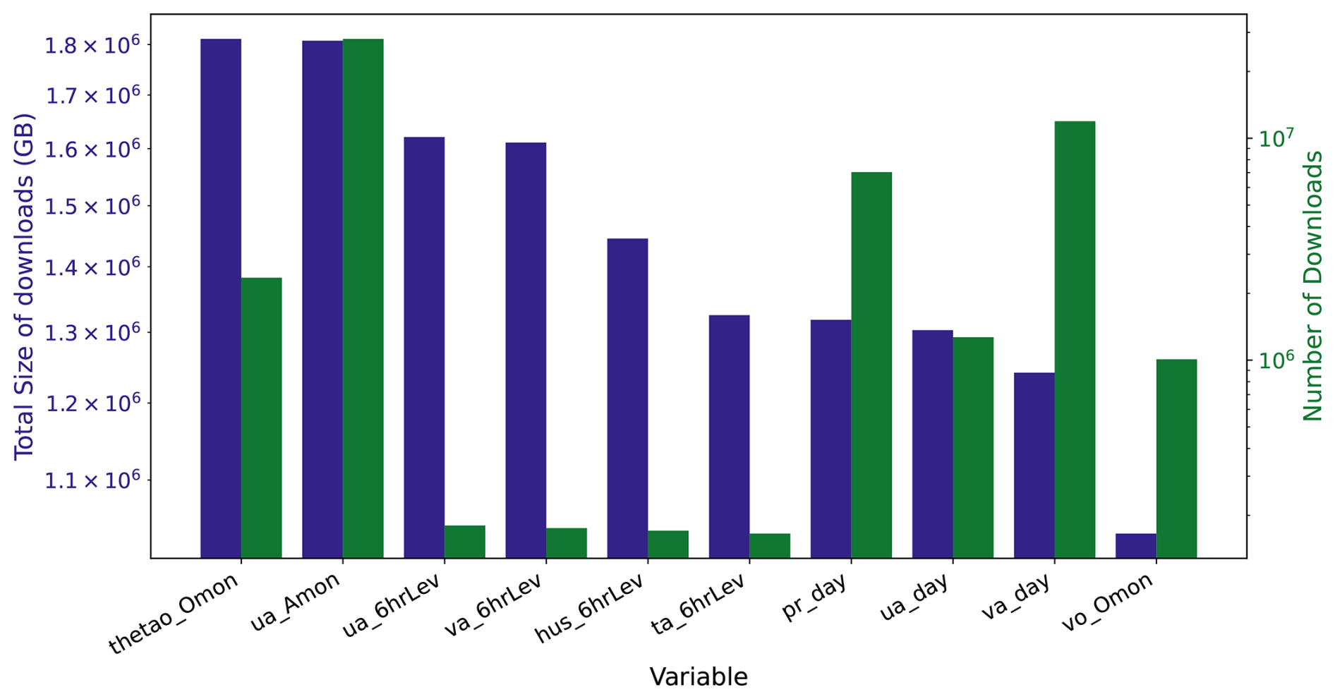
Figure 3 shows the top 10 most downloaded variables by size. The pattern is not the same as for number of files, as total size favours files that are 3-dimensional, have more vertical levels and more time steps. These factors allow thetao_Omon to take the top of the chart in terms of total size of downloads (left axis). In general, temperature and wind variables are the most downloaded.

Figure 3 Total size in GB and number of downloaded files for each unique variable.

Another influencing factor is the amount of data available on ESGF nodes for a given variable. To control for this, we define the ratio

$$\begin{array}{}\text{(1)}& R={\displaystyle \frac{\mathrm{total}\mathrm{size}\mathrm{of}\mathrm{dat}\mathrm{downloaded}}{\mathrm{total}\mathrm{size}\mathrm{of}\mathrm{data}\mathrm{available}}},\end{array}$$

to understand the usage rate of a variable.

Figure 4 shows the distribution of R for every variable. A bit more than a quarter of the 1811 variables have a ratio smaller than 1, meaning that more data was available than downloaded. (Here, a quarter of the variables does not mean a quarter of the size of the full archive as some variables are uploaded less than others.) Table S3 lists the variables that have a R below 1. By definition, this could still mean that some of the variables were downloaded multiple times for a given model and experiments, but never for others as R provides only a general impression.

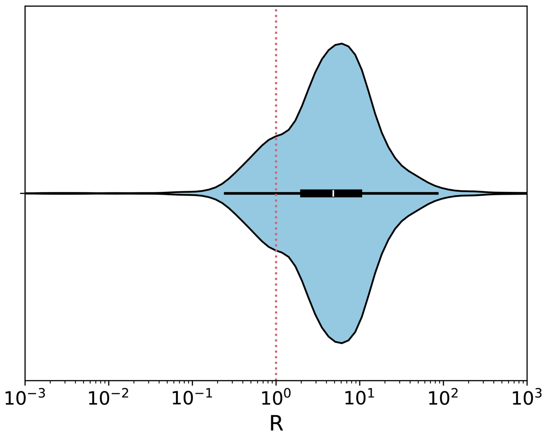
Figure 4 Distribution of the ratio of data downloaded over data available for each variable. Red line at R=1. The x axis has been cut for readability.

On the other side of the spectrum, for high R (Table S4), we see some variables that top the ranking in the size of the downloads. One such variable is ua_Amon (R=955). The size of the uploads for this variable (denominator of R) is very high, but so is the size of the downloads (numerator of R). On top of this, R highlights variables with a very high download rate that did not have many uploads and were invisible to previous analysis, e.g. rsu_Efx (R=1353). The mean of R is 21 and the median is 5. There are also 18 variables with ∼0 GB of downloads, that is datasets with less than 0.01 GB, which are not shown.

3.2 Experiments and activities

Among the different MIP activities, CMIP and ScenarioMIP stand out in the download statistics, both according to number of downloads and download volume (Fig. 5a). CMIP and ScenarioMIP represent core experiments to which modelling centres contribute. As a result, there is overall a larger amount of data available to download for these activities in comparison to most other MIPs. CMIP covers the common experiments of CMIP6, the historical simulation as well as the DECK experiments (Eyring et al., 2016). These, especially the historical and piControl experiments, represent most of the CMIP downloads and often provide a point of comparison for studies using other experiments (Fig. 6).

Figure 5 Most downloaded experiments per MIP according to (a) total number of downloads and (b) download size. Explicitly shown are only experiments with >10 % share in downloads, the rest are summarized as “other”.

Figure 6 Share in number of downloads (dark blue) and download size (light blue) for (a) all intercomparison projects and (b) with the six largest excluded. Sorted from largest number of downloads to smallest. Note that the sorting according to number of downloads and download size differ.

For ScenarioMIP, simulations ssp245 and ssp585 have the largest share, although the orer switches between number of downloads and download volume, followed by ssp370 and ssp126, which also switch in order between measures (Fig. 6). Between experiments, the contributing modelling centres and models differ. For some models, each simulation year is uploaded individually for one experiment (e.g., EC-Earth), whereas files available for download by other models cover decades or centuries. Some modelling centres also extended their experiments beyond 2100 CE, leading to increased download sizes. The size of ensembles further differs between different modelling centres and models. As such, differences between the statistics according to number of downloads versus download size between experiments can occur when different models conducted different experiments with varying ensemble sizes. Furthermore, for different experiments and models, data might be available at different resolutions (temporal and spatial) or for a different set of variables (e.g., additionally available 3D fields for one experiment would increase the amount of data downloaded much more than the number of files).

HighResMIP, AerChemMIP, DAMIP and DCPP complete the six most downloaded activities (Fig. 5). These are around an order of magnitude smaller in both number and volume of downloads in comparison to CMIP and ScenarioMIP, but stand out with respect to all other activities. Among the remaining activities, relative sizes vary between number and volume of downloads (Fig. 5b). Some activities have clear main experiments, e.g., DCPPA-hindcast for DCPP with a share larger than 80 % according to both measures in comparison to the 23 other DCPP experiments. For other MIPs, several experiments are similarly relevant in the download statistics, as is the case for FAFMIP, PMIP and RFMIP among others.

Overall, availability of data reflects different priorities between modelling centres, which will for example contribute only to MIPs matching their priorities on top of the core experiments from CMIP and ScenarioMIP. Download statistics are also correlated to the amount of data available for download and when that data was added to repositories. For a thorough analysis of the effects of data availability, download statistics over time would be needed, which were unavailable for our analysis.

3.3 Sources and institutions

Figure 7 illustrates ESGF usage metrics for climate models, called “source” in the CMIP CVs, categorized by their total download size and total number of downloads and binned accordingly. Here, we note that model data that were hosted by untracked nodes (either for a portion of or the whole sampling period) might be under-represented in the results. EC-EARTH3, IPSL-CM6A-LR and MPI-ESM1-2-HR are the most downloaded sources in terms of download size. EC-EARTH3 leads by a wide margin when considering number of downloads, followed by EC-EARTH3-VEG and MPI-ESM1-2-LR. The elevated download count for EC-EARTH3 may be partially explained by its extensive number of files, as files are provided individually for every simulation year, potentially inflating download numbers.

Figure 7 Total size in GB (blue) and number of downloaded files (green) for top 20 model configuration according to total download size.

To better understand differences between download numbers and sizes within the same and between sources, we conduct an analysis comparing the available datasets for 2 different sources, EC-EARTH3 and CESM2, for a specific variable and table and a specific activity and experiment. We choose the tas variable at monthly frequency for the CMIP activity and the historical experiment. For EC-EARTH3, 9450 files are available on the ESGF nodes included in the CMCC monitoring nodes, accounting for a total of 41.67 GB with a mean file size of 4.4 MB. Among the historical simulations, EC-EARTH3 provides 12 main members covering the period 1850–2014 and 50 additional members covering the period 1970–2014. All available historical simulations are divided into yearly files, explaining the high number of available files and download statistics. When looking at the individual files on the ESGF node search, most of the files have a size of ∼4.51 MB. The equivalent file size of a historical member covering the entire period for a 2D variable is ∼745.8 MB. CESM2 provides 26 files, for a total size of 2.49 GB. 11 members are available, all covering the period 1850–2014. The simulations are chunked following 2 different data saving strategies: they can either be divided into 4 different files of 50 years (1850–1899, 1900–1949, 1950–1999) and 1 file of 15 years (2000–2014) or only 1 file covering the entire period (1850–2014). Whatever the storage strategy, one member covering the entire period has an equivalent file size of ∼231.8 MB, which is 3.2 times smaller than for EC-EARTH3. This difference can be explained by the resolution (although similar in historical simulations), by the precision of output values and the compression technique for the files, among others. This example highlights how both storage decisions like file chunk size and modelling choices like the resolution will impact and skew download statistics and comparisons involving simulations from different models and institutions. As such, the comparison between EC-EARTH3 and CESM2 shows the possible range in download statistics due to these storage decisions.

Analysing the institutions involved in CMIP can be a bit tricky. Some climate models are developed by a single modelling centre, while others are developed by consortia. For instance, the Institut Pierre-Simon Laplace (IPSL) centre develops 10 different configurations of their climate model, which are considered as different sources. In contrast, a consortium of different European laboratories and national research centres shares the burden of developing and producing simulations of 10 configurations of the EC-Earth model. Some centres also partner with other laboratories only for specific configurations of their model. For instance, the Met Office Hadley Centre (MOHC) develops and produces its own climate model, HadGEM3-GC31, with different configurations related to different grid resolutions. But it also produces two other models (UKESM1-0-LL and UKESM1-1-LL) in collaboration with two other centres, the National Institute of Meteorological Sciences–Korea Meteorological Administration (NIMS–KMA) and the National Institute of Water and Atmospheric Research (NIWA). Lastly, some modelling centres may produce just one model participating in a single CMIP activity, while other centres produce different models that may participate in many different activities. The Seoul National University develops the SAM0-UNICON model which participated only in two activities, CMIP and ScenarioMIP. The Canadian Centre for Climate Modelling and Analysis (CCCma) develops the CanESM5 model (among three models) which participated in 16 different activities (https://pcmdi.llnl.gov/CMIP6/ArchiveStatistics/esgf_data_holdings/, last access: 15 November 2025). The contribution of each modelling centre, but also of each source, to CMIP activities is therefore very diverse and cannot be easily compared. Combined statistical data on downloads, for example by source and experiment, would enable this analysis to be refined.

3.4 Countries, regions, and continents

Figure 8 illustrates the data volumes published and downloaded within specific countries or regions. The teal bars indicate the total amount of CMIP6 data published by all climate modelling centres based in the indicated location, while the blue bars indicate the total amount of CMIP6 data downloaded by users. Similarly, Fig. 9 classifies published and downloaded data volumes by continent. Data volumes associated with the publication of EC-Earth simulations were divided equally among countries hosting a core partner organisation of the EC-Earth consortium (Denmark, Finland, Ireland, Italy, Netherlands, Spain, Sweden).

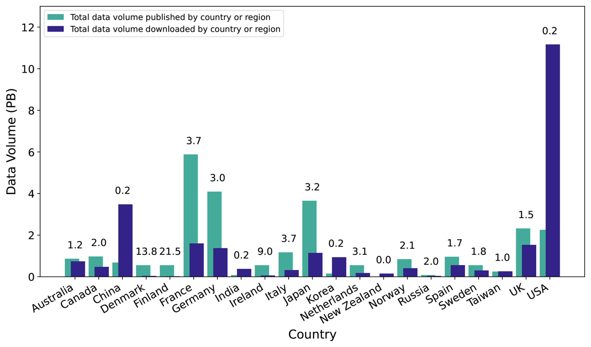
Figure 8 Sum of CMIP6 data published by organisations in a given country or region (teal) and the sum of all CMIP6 downloads by users in the country or region (dark blue). Numbers above the bars are the ratios of the two bars.

Figure 9 Same as Fig. 8 but for continents. No data was published by African and South American organisations.

The two figures show a clear trend of European countries publishing much more data than they download, double on average, and the two largest European publishers, France and Germany, in particular, publish 3.7 and 3.0 times more than they download. Unsurprisingly, the three major publishers and “consumers” in Europe are France, Germany, and the UK, who develop two or more ESMs each, and operate the three major ESGF nodes in Europe. The high concentration of nodes in Europe may explain the low number of downloads in Europe. Indeed, the French, German and British nodes (IPSL, DKRZ and UKRI) are replica nodes that offer untracked direct access to their data pool for members of their institutions. This unmonitored data might skew the download statistics by country. Indeed, the IS-ENES3 project found that the increase in the number of ESGF users in 2020–2021 was mainly driven by non-Europeans and associated this result with an increased use of the direct access to ESGF replica nodes data pool by European users, instead of download from the ESGF system (Kindermann et al., 2022). The publication-to-download trend is inverted in North America, where downloads are 3.7 times publications. This signal is dominated by the USA, where by far the largest data volumes are downloaded, at around 11 PB, or 5 times the data volume published. In comparison, the USA publishes similar volumes to the UK, but downloads 7 times more data.

Figure 10 (a) Total number, and (b) number per capita of downloads from ESGF amongst the countries or regions with highest usage by each metric.

Asian countries or regions show differing behaviours, with China, Korea, and India downloading more, Japan publishing more, and Taiwan displaying similar volumes between both. China, in particular, despite ranking behind several countries in terms of data published, is the second largest “downloader” of data after the USA. In Oceania, publication and downloads balance out exactly.

By total number of downloads, China is responsible for the largest amount of downloads at 69 million downloads, followed by the USA with 40 million, and Japan with 8.6 million (Fig. 10). Per capita, Switzerland is the highest usage country or region, with over 0.6 downloads per person, followed by Norway and Sweden (Fig. 11). Many countries see less than 1 download per 1000 people, particularly in Africa, Eastern Europe, and Central Asia. There are around 100 times more downloads per capita amongst the highest usage countries, such as Switzerland, compared to even the top-usage lower-middle income countries, such as Argentina. Many countries around the world, particularly in Africa and Central Asia, have almost no interaction with the ESGF archive, with less than 1000 cumulative downloads of CMIP6 data.

Figure 11 World map showing downloads from ESGF per 1000 population. Countries and regions without ESGF download statistics are marked gray.

4 Other CMIP6 data providers

CMIP6 data is also available on Google and AWS clouds for data-proximate computing, as well as on C3S for download (Sect. 2). Figure 12 shows the most and least downloaded variables on ESGF and if those variables are available or not (black/white, respectively) at the other providers. Each row represents a variable, following the ESGF ranking of download volume (as in Fig. 1). Highlighted are the top 15 most and least downloaded variables (Fig. 12a and b). Figure 12c shows the availability for all variables (also in order of ESGF downloads). Many of the most popular variables on ESGF are available on other sources, but it is not a perfect match. For example, the most downloaded variable on ESGF, thetao_Omon, is not available on C3S and a very low ESGF download variable, sosga_Odec, is available in the Google cloud. It could be of interest to provide some of the missing most downloaded variables in the future, although different user communities may have different needs, particularly in terms of realms and frequencies. Conversely, the figure shows variables that got barely any downloads on ESGF, which other platforms could avoid having to curate, transform and upload if not specifically requested by their user base. Since space is limited, it might be more useful to replace these with a variable that are more downloaded on ESGF.

Figure 12 Availability of variables on Google, AWS and C3S, listed in order of ESGF downloads.Variables that are available are shown in black, variables that are not available in white. (a) Top 15 most (top panel, similar to Fig. 3) and least (bottom panel) downloaded variables on ESGF. (b) Availability across data providers for these variables. (c) Availability of all variables across data providers.

To try to understand the user communities of these other sources, we also consulted the download and access statistics available for each of them. Unfortunately, no statistics were recorded for the Google cloud. We present our analyses for the statistics of AWS S3 in Sect. 4.1 and for C3S in Sect. 4.2.

4.1 AWS S3

During the analysis period, the AWS S3 access statistics recorded approximately 12.8 million object-level requests, corresponding to an average of about 0.8 million requests per month. However, the temporal distribution of requests is highly uneven, as approximately 92 % of all recorded requests happened over only 28 individual days. Data transfers also occurred during concentrated periods of high activity as almost all accesses were recorded in mid-September 2022, in mid-December 2022 to early February 2023 and from April to May 2023. These peaks in activity may indicate a sporadic but intense use of the platform, possibly related to the occurrence of major scientific meetings.

Several factors complicate the analysis of the AWS S3 statistics, foremost are the limited metrics available, which are count of requests, unique client IP addresses and the amount of data transferred. However, a data transfer does not occur for every request or connected IP, as these might correspond to metadata queries rather than the transfer of data. Different types of operations from metadata operations to data streaming from the cloud-based computing environments and explicit data downloads can be recorded in the access statistics and are impossible to disentangle, although they indicate an overall interest in the stored data.

4.2 C3S

C3S keeps a log of the received requests (Sect. 2.3). Figure 13 shows the ranking of variables on C3S by number of requests and number of users. Here, a request can include any number of files as the CDS requests are not constrained by file structure and storage as they are on ESGF. These types of statistics can thus give a more accurate picture of the usage of a dataset.

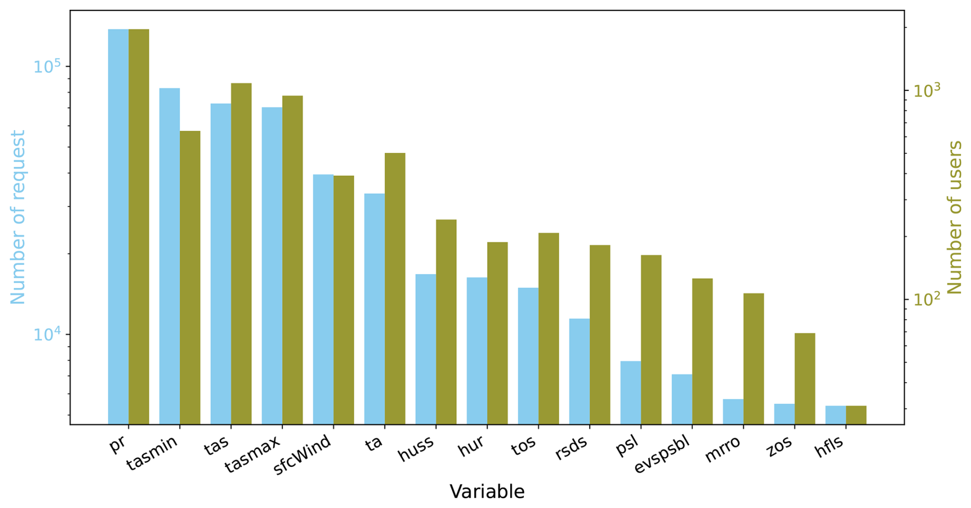
Figure 13 Number of requests and users on C3S for each variable. This includes monthly, daily and fixed frequencies.

Statistics for C3S (number of requests and users) cannot be directly compared to number of files or size of downloads from ESGF, but the order of the variables can be compared. Temperature, wind and precipitation are highly requested/downloaded for both archives. However, the eastward wind component that is in second position for ESGF does not make the top 15 most requested variables for C3S. This might be because it is only available at monthly resolution on C3S, while other variables are also available at a daily resolution.

Figure 14 presents the number of requests and users of C3S for each model. The orders by request and by users are quite different from each other. This might point to some models, like EC-EARTH3-VEG-LR, being highly requested with a small number of users that are making many requests. Further, ACCESS-CM2, the most popular model, is the first model listed on the website. This might create an artificial demand by users who do not have a preference for any specific model. Note that the availability of data also affects the ranking. Figure 14 only shows the top 15 models, but there are 58 models available. The top 15, in terms of number of requests, all have more than 235 datasets available for each model, while the bottom 15, in terms of number of requests, all have less then 89 datasets available. Generally, the ranking of models by number of request on C3S does not match the ranking by number of downloads for ESGF.

Figure 14 Number of requests and users on C3S for each model. Only showing the top 15. The numbers in parenthesis represent the number of datasets (unique variable, frequency and experiment) available.

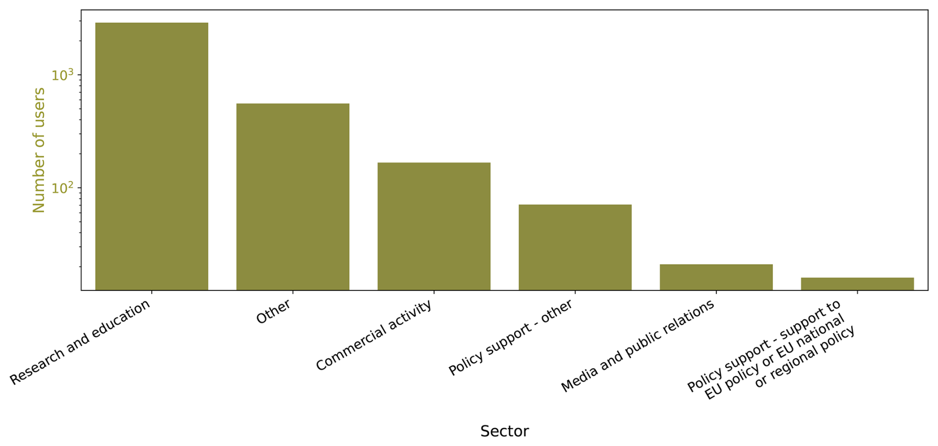
The location of users is also quite different between C3S and ESGF. Figure 15 lists the top 10 countries where most requests are originating. The ranking is based on C3S data on users and on ESGF data on number of downloads. Large users like the USA and China appear in both lists, but in general countries in the Global South are more likely to be in the top for C3S, whereas countries in the Global North are more likely to be in the top for ESGF. One possible hypothesis is that users with less resources are more likely to use a service where the data can be subset before download. However, as discussed in Sect. 3.4, missing data from untracked shared institutional resources might modify the geographical results for ESGF. More detailed statistics data is available about C3S users. Figure 16 shows their sector of activity. Unsurprisingly, Research and Education is taking the top spot. Unfortunately, this information is not available for other data sources. Hence, it is not possible to compare differences in communities between data providers.

Figure 15 Map of countries and regions that are in the top 10 users from ESGF (red), C3S (blue) or both (purple).

Figure 16 Number of users of C3S for each sector.

5 Use cases of CMIP data

5.1 Scientific research

The impact of CMIP6 on scientific research can be estimated by the number of citations of CMIP datasets in the literature. For the first time in CMIP6, a citation service for the data was created in order to follow best practices in open science and to give the proper credit to the modellers. DOIs were minted for each model-activity and each model-experiment combination (Stockhause et al., 2015). A total of 3009 entries were registered. The sum of all citations for all DOIs amounts to 27 456, which includes several citations for individual publications. We note that this number is likely incomplete. Indeed, the citation of model-activity combinations is particularly low, although the terms of use of the data (https://pcmdi.github.io/CMIP6/TermsOfUse/TermsOfUse6-2.html, last access: 15 November 2025) indicate that users of the data should cite each dataset. Still, some publications might have only cited the description papers from the CMIP6 special issue (https://gmd.copernicus.org/articles/special_issue590.html, last access: 15 November 2025). Indeed, the CMIP6 overview paper (Eyring et al., 2016) has been cited 6619 times and the paper describing ScenarioMIP (O'Neill et al., 2016) 2923 times. A thorough analysis of appearance of CMIP in the literature has been published in Ju et al. (2025).

Keeping this caveat in mind, Fig. 17 shows the number of citations compared to the total size of downloads for each model and experiment on ESGF. The citation numbers for all the model-activity combinations were summed over the activities and the experiment-model combinations were summed over the models. According to this measure, the most cited model is IPSL-CM6A-LR and the most cited experiment is historical. In general, we can see that a dataset with high downloads also seems to have a high citation number, though there is a lot of variability, especially for models. For example, EC-Earth has the largest amount of downloads, but only 35 citations. This analysis is intended to be exploratory. Due to the low number of citations, we can not reach any robust conclusions here. A more thourough analysis of CMIP DOIs can be found in Kindermann et al. (2023).

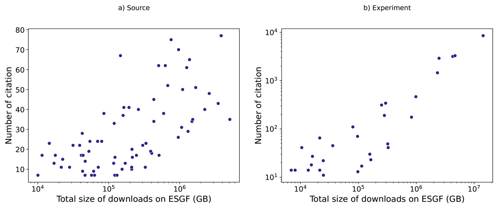
Figure 17 Total download size on ESGF versus number of citations. (a) Citations for source. (b) Citations for each experiment, calculated as the sum of all DOIs that refer to a given experiment.

CMIP6 also put in place a publication hub (https://cmip-publications.llnl.gov, last access: 15 November 2025) for authors to register their papers using CMIP6 data. However, very few papers have been registered and the hub is offline at the time of writing this manuscript.

5.2 Informing society and downscaled datasets

CMIP6 data also serves to inform society, for example through the IPCC assessment reports. At the regional scale, the resolution and biases of the CMIP models are often an obstacle. In that case, a supplementary step is necessary: downscaling, creating new datasets from CMIP data. Hence, a single download of a CMIP dataset to create a downscaled dataset can undersample the use of the CMIP information through this new dataset. Indeed, the overview presented in this manuscript is ignoring the downscaling community, intensive users of CMIP information, adding to the underestimation of overall use.

For dynamically downscaled data, simulation data from CMIP6 Global Climate Models (GCMs) is downloaded once from ESGF to drive Regional Climate Models (RCMs). The CORDEX project (Gutowski et al., 2016) coordinates efforts of dynamical downscaling and provides a list of registered RCMs (https://github.com/WCRP-CORDEX/cordex-cmip6-cv/blob/main/CORDEX-CMIP6_source_id.json, last access: 15 November 2025). Some of the CORDEX project data is also hosted on ESGF nodes and usage statistics are available through the ESGF Data Statistics service. They total 3 319 978 GB and 9 238 679 files downloaded. Due to the delayed timing of CORDEX phases with respect to CMIP phases, these numbers refer to downscaled CMIP5 simulations. Further, some regional centres do not distribute their data through ESGF nodes and are therefore not counted in this analysis.

Regional climate models require large resources to run as well as specific GCM outputs, including some CMIP outputs to be initialised and forced at boundaries. As such, it is not always possible to perform dynamical downscaling. Hence, many groups in need of high resolution data turn to statistical downscaling. Using a high resolution observational dataset and statistical approaches, GCM data can be brought to a finer resolution. This method also has the ability to adjust some of the biases of the GCM, which is often critical to run impact models. A similar bias-adjustment can also be performed for dynamical downscaling. There is no official record of statistical downscaling efforts based on CMIP data. As a result, usage statistics cannot be estimated as downscaled datasets are often distributed locally by the organisation that created the dataset. As a starting point, we list a few statistical downscaled datasets in the Supplement Table S5. CORDEX has recently proposed a framework to bundle efforts for statistical downscaling (https://cordex.org/wp-content/uploads/2024/04/Second- order-draft-CORDEX-experiment-design-for-statistical-downscaling-of-CMIP6.pdf, last access: 15 November 2025), which could provide a more complete record in the future.

6 Conclusion: lessons for the future

To better understand the usage of CMIP6 data, we gathered statistics on usage, access and downloads from major sources (ESGF, Google, AWS, C3S), focussing on ESGF with the most extensive available statistics. Besides the lessons learned from the results of our analysis, the analysis we were unable to do due to limitations in the availability of usage statistics also proved informative. We present these lessons here along with suggestions for future improvements of statistics collection and CMIP publication.

First, for a quarter of the variables on ESGF there is more data available than data downloaded. To optimize storage use and reduce the carbon footprint, it may be worthwhile to examine these less-downloaded variables more closely and revisit resource allocation. Alongside other metrics (like scientific value, community interest and others), these download statistics could help determine whether such low-usage-rate variables could be limited to lower frequencies, uploaded at higher compression or shared in a different way to the interested community. Table S3 provides a list of those variables. Juckes et al. (2025) have further proposed a list of 135 variables to prioritize in CMIP7, which should be viewed in the context of the ongoing work on the data request (Mackallah et al., 2026).

Second, cleaning the ESGF data showed that 1000 TB of erroneous files (with metadata that did not match existing CVs, see Sect. 3.1) were downloaded by users. These issues probably led to inefficiencies in users' workflows lowering the usability of CMIP data and making reproducibility harder. Indeed, there was a proliferation of “fixer tools” that were all doing the same task but were unique to a small group of users. Institutional copies of the data were also probably fixed internally repeatedly. The newly created ESGF Quality Assurance/ Quality Control (QA/QC) will most likely significantly reduce the extent to which this issue occurs in CMIP7 and we strongly support this effort.

Third, there is a notable difference in downloads based solely on how a dataset was stored, e.g., as one large file versus one file per year. Prescribing a uniform format to store the data could potentially result in data originating from different models being used more consistently by users, in addition to making the usage analysis easier to interpret. From a data producer point of view, prescribing a uniform file formatting, associated with an optimised compression and precision required to store each variable, could reduce storage requirements and at the same time make data more accessible for users. The lessons learned on “data request and transfer modelling” during the Primavera H2020 project (https://www.primavera-h2020.eu/assets/media/uploads/Documents/project/primavera_d9.6_final.pdf, last access: 9 September 2026) and the recommendations on atmospheric variable compression (Klöwer et al., 2021) could serve as a basis for future recommendations, especially with regard to the “high volume” variables suggested in Juckes et al. (2025) for CMIP7.

Fourth, sources other than ESGF can provide only a subset of the CMIP data available, often due to resource constraints. Indeed, cloud sources are often community and volunteer built prototypes. In the future, our analysis could thus help choose which data to include in their subsets, although the ESGF download rate is not a perfect indicator as users of different sources might not have the same interests or capacities.

Lastly, it was challenging to study the impact of the datasets through the citation of the DOIs as it is unclear how often these are actually used in publications and we suspect that many publications are not citing the data DOIs. Clearer instructions on citation on the CMIP user guidance page, could help enhance proper citation practices. Also, the new concept of “complex citations object”, which links multiple digital objects through a single DOI, could make it easier to cite many datasets (Agarwal et al., 2025).

Overall, this project showed that many types of analysis are impossible using the currently available download statistics, in particular for data providers other than ESGF. In the following, we suggest a few improvements that would help future analyses of this kind.

For the ESGF data, the openly available ESGF Data Statistics provide only a snapshot of tracked statistics. In order to perform a more detailed analysis, it would have been very valuable to have access to cross-variable statistics, e.g., downloads of variables for a given experiment, or changes over time. A public API to query such a database would facilitate the process of retrieving data and producing analyses. While potentially valuable within the scope of our work, we do acknowledge that developing such a database with cross-variable statistics and a public API would require significant resources.

While C3S provides information on a user's sector, such information is unavailable for ESGF, where the general user profile is likely different. Tracking such data might however be difficult considering privacy concerns. Further, such data on users is easier to gather for C3S, which requires an account, which is not the case for ESGF. Still, the sector of the users could be asked when creating a Metagrid account. Another concept that ESGF could take from C3S is to gather statistics at the dataset level, rather than at the file level. Statistics at the dataset PID (Persistent Identifier) level or usage by simulation year as done by Sigmond et al. (2023) would be another possibility. These options would clearly require a lot of work, but would allow for a more accurate picture of usage, unconstrained by size and archiving format. This would provide a better understanding of the differences between resolution-based and equivalent-variable models, thereby enabling more effective process optimization, without limiting modelling centres' ability to use files of a manageable size based on their own criteria and to enhance the user experience.

For data hosted by Google there are currently no access statistics tracked and logs of AWS data access are limited. Since these archives address different user groups and needs, tracking data access at all or more extensively could provide valuable information in the future. Cloud services allow data to be streamed (allowing for only the data relevant to the analysis to be accessed), as well as downloaded locally. Statistics that distinguish between these two practices might be particularly insightful. However, we note that statistics for size of data streamed will always appear smaller than size of data downloaded (either through the cloud or ESGF) as only the chunks that are used will be counted. Statistics on the number of files might just be inappropriate for streaming. If counting access by dataset or by simulation year as suggested above, it is unclear if a download of the full data should be counted in the same way as access to only a few grid points. In the future, we are expecting that more and more CMIP data will be accessible through the cloud (Mizielinski et al., 2026). Hence, it will become more important to log streaming access to be able to fully capture the use of CMIP7 data.

Another very important source category that is not tracked are large institutional archives, such as the replica pools provided in conjunction with many ESGF nodes. Because of this, we are missing many users in Europe. For a more thorough understanding of usage, institutional statistics would thus need to be gathered and made publicly available.

Finally, we suggest a registry for statistically downscaled dataset. This would allow a more complete overview of the use of CMIP data in the decision-making space, and it could be complemented with data usage and download statistics provided by individual groups.