Variational Stokes method applied to free surface boundaries in numerical geodynamical models using the staggered-grid finite-difference discretisation

Accurately and efficiently modelling topographic evolution is a key challenge in geodynamic modelling, which requires the solution of the Stokes equations with free surface boundary conditions. While finite difference methods on staggered grids, as used in geodynamic modelling codes such as StagYY, I3ELVIS and LaMEM, offer strong computational performance and compatibility with multigrid solvers, the use of fixed Eulerian grids complicates the implementation of realistic, deformable free surfaces. Two existing methods are available to model free surface boundary conditions in such codes: the commonly used sticky-air method, which suffers from limitations relating to high viscosity contrasts, and the “staircase” method, which improves upon the sticky air method by imposing free surface boundary conditions at cell boundaries.

To address the limitations of existing methods of implementing free surface boundary conditions, this study investigates an alternative variational discretisation of the Stokes equations that uses volume fractions to represent a smooth surface within a fixed Eulerian grid, allowing the imposition of accurate free surface boundary conditions while allowing it to bypass the limitations of existing free surface discretisation methods.

The variational Stokes method is demonstrated to be an accurate and computationally efficient alternative to existing methods. It reproduces results comparable to existing methods while reducing computational cost and enabling broader applications, including non-zero surface tractions, complex surface loading, and compatibility with 3D spherical geometries.

1 Introduction

The Stokes equations are the governing equations of mantle convection, and their solution is the key goal of numerical geodynamic models. Numerous discretisation methods exist for solving these equations numerically, including the finite difference method, finite volume method, finite element method, and spectral element method. Among these, the finite difference method on a staggered grid, which is equivalent to the finite volume method, is often used in geodynamic modelling codes (e.g. Patankar, 1980; Ogawa et al., 1991; Tackley, 1993; Trompert and Hansen, 1996; Gerya and Yuen, 2007; Tackley, 2008; Gerya et al., 2015a; Kaus et al., 2016; Duretz et al., 2016) due to its simplicity in discretising the governing equations and compatibility with efficient multigrid solvers in both 2D and 3D.

A key component of the finite difference method is the transformation of continuous differential equations into a discretised system that can be solved numerically on a fixed Eulerian grid. However, while the finite difference method offers computational efficiency and stability, it introduces challenges when modelling free surface boundary conditions, which are essential for the accurate modelling of topographic evolution on planets. The fixed grids used by the above geodynamical modelling codes are not readily adaptable to modelling surface deformation, necessitating alternative techniques to account for free surface boundary conditions.

Modelling free surface boundary conditions on a fixed Eulerian grid requires two key components: a method for tracking the location of the surface over time, and a method of discretising the Stokes equations in a way that incorporates the free surface boundary condition, with this study focussing on the latter.

The most straightforward approach for achieving this is the so-called sticky air method. In this method, a relatively low-viscosity layer is added above the rock layer of interest to represent the air (Gerya (2019) and references therein). The presence of this low viscosity layer allows the surface to deform relatively freely and thus approximate a true free surface boundary condition; however, computational limitations on viscosity contrast mean that the air layer is unable to be set to the extremely low viscosity of actual air. Hence, the use of a higher viscosity “sticky” air layer. Although conceptually simple, this method presents several drawbacks, which are discussed in Sect. 2.1 below.

To address the limitations of the sticky air method, Duretz et al. (2016) introduced a novel discretisation method, henceforth referred to as the “staircase” method. This approach eliminates the need for modelling a sticky air layer by applying zero Dirichlet boundary conditions on pressures and velocities within the air layer, while allowing the surface itself to deform freely via alternative boundary conditions in the interfacial cells. Although this method improves numerical performance by allowing for a relatively thinner air layer and avoiding the viscosity contrast inherent in the sticky air method, it introduces its own set of challenges, which are discussed in Sect. 2.2 below.

Given these challenges, there is a need for a more robust and efficient method to discretise the Stokes equations for the modelling of free surfaces. Such a method should satisfy several key criteria:

• Remove or minimise the viscosity contrast dependence inherent in the sticky air method.

• Remove or minimise the necessity for a thick air layer.

• Enable efficient and stable solutions in both 2D and 3D, using both direct and iterative (multigrid) solvers, and on both Cartesian and non-Cartesian grids.

A promising direction in this field is the variational Stokes method, introduced by Larionov et al. (2017). This method is conceptually similar to the aforementioned staircase method in that it eliminates the need to explicitly model a low viscosity sticky air layer. However, instead of a discrete staircase representation of the free surface, this method proposes a smooth representation of free surfaces through the use of volume fractions, which can be readily computed in one of several ways, including a volume of fluid method or a direct Lagrangian representation of the surface. We discuss the implementation of this method (using StagYY Tackley (2008) as an example code), the comparison of this method to the existing sticky air and staircase methods, and the potential applications of such methods to global scale numerical geodynamical models. While Larionov et al. (2017) model viscous animal-shaped objects and falling streams/blocks/layers of viscous fluid, we here demonstrate the applicability of the method to geodynamical modelling of the solid Earth with a free outer surface using a staggered-grid finite difference discretisation and a multigrid Stokes solver, with systematic tests showing that it has some advantages to the currently-used sticky air and staircase methods.

Larionov et al. (2017) provide an extensive review of related methods. Furthermore, in the (finite Prantl number) fluid dynamics community, a commonly used approach is the immersed boundary method (for a review see Verzicco, 2023), in which volumetric forces are added to enforce the boundary conditions at the interface. For finite element discretisations the CutFEM method (see Burman et al. (2025) for a review and comparison to other methods) results in a modified weak form of the equations accounting for the interface conditions inside cut elements.

2 Existing methods

Two methods for numerically modelling a free surface in an Eulerian staggered finite-difference grid are currently used in the geodynamical community: the sticky air method (Schmeling et al., 2008; Crameri et al., 2012)), and the staircase method (Duretz et al., 2016).

2.1 Sticky air method

The sticky air method involves the use of a layer of low viscosity material at the top of the model domain, which represents an air layer within which the surface can freely deform. At standard temperature and pressure, real air has a viscosity of approximately 1.8 × 10⁻⁵ Pa s, over 20 orders of magnitude lower than typical mantle rock viscosities, which typically range between 10¹⁹–10²⁰ Pa s. However, the naive solution of applying such a large viscosity contrast to a numerical model would cause the resulting linear system to become extremely poorly conditioned, resulting in low quality results and poor numerical performance (Gerya, 2019).

For this reason, an effective air viscosity is used that is significantly higher than that of actual air, typically on the order of 1000 times lower then the viscosity of rock in the model, resulting in a modelled viscosity on the order of 10¹⁶–10¹⁸ Pa s. This enhances numerical performance significantly, while still approximating free deformations of the surface. However, the sticky air approach suffers from limitations in cases when the viscosity contrast or the thickness of the air layer is insufficient. For certain analytical cases, simple criteria can be derived which can be used to determine whether the surface will be traction free as a function of the model geometry and viscosity contrast (Crameri et al., 2012). These criteria take the form:

$$\begin{array}{}\text{(1)}& A{\displaystyle \frac{{\mathit{\eta }}_{\text{air}}}{{\mathit{\eta }}_{\text{rock}}}}{\left({\displaystyle \frac{L}{h_{\text{air}}}}\right)}^{\mathrm{3}}\ll \mathrm{1},\end{array}$$

where η_air and η_rock are the characteristic viscosities of the sticky air and underlying rock, h_air is the sticky air layer thickness, L is a characteristic length (typically the mantle thickness in global scale models). The constant A is a model-dependent parameter which can be derived analytically for a number of simple scenarios (Crameri et al., 2012). From this relation, it can be concluded that both air layer thickness and viscosity contrast must be sufficiently high in order to approximate a traction-free surface.

The presence of a sticky air layer introduces several issues. The first issue is the requirement to have a thick layer of low viscosity material. This inherently increases the model domain size, and thus decreases numerical performance by having to solve for a greater number of degrees of freedom than are otherwise necessary (Duretz et al., 2016). Furthermore, as the fluid velocities within the low-viscosity air layer are often higher than the high-viscosity rock, timesteps may be limited unnecessarily in order to accommodate deformation of the air layer. As the air layer itself is uninteresting for researchers, serving only to enable a free surface boundary condition, this implies that computational effort is wasted.

The second and most prominent issue relates to the sharp viscosity contrast necessary to obtain accurate solutions when using the sticky air method. The introduction of viscosity contrasts into a model makes the discretised form of the Stokes equations poorly conditioned, and generally more difficult to solve. While direct solvers, which are more commonly used in 2D models, are not as sensitive to sharp viscosity contrasts, iterative solvers including the iterative multigrid approach used for solving 3D models are strongly affected by them. This increase in computational cost has contributed to making use of the sticky air method, and due to the ubiquity of the method, free surface modelling in general less desirable when using 3D models.

2.2 Staircase method

Seeking to overcome the limitations of the sticky air approach, Duretz et al. (2016) proposed an alternative method of modelling surfaces in finite-difference Stokes models, referred to here as the staircase method. This approach eliminates the need for a sticky air layer by avoiding equations in the air domain and instead modelling a free surface boundary condition using modified boundary conditions at interfacial cells. In this way, it is possible to model a true free surface boundary condition without the need for a thick, low-viscosity sticky air layer.

The method requires a method of tracking the location of the free surface. While Duretz et al. (2016) use a simple marker chain to directly track the interface location over time, in principle any method of tracking free surfaces, which also inclulde the marker-in-cell method and volume of fluid method, could be used. For a comparison of the performance of these methods see Gray et al. (2026a, b).

In the staircase method, computational cells with a centre point that is below the location of the surface are considered to be fluid (i.e. rock for geodynamic applications) cells, while cells above are considered to be air cells. These two cell classifications imply the existence of an interface between the cells which follows cell boundaries, and which therefore follows a staircase pattern when using a Cartesian grid (Fig. 1). In air cells that are not directly adjacent to the interface, no equations are solved and the pressure and velocities are set to zero through Dirichlet boundary conditions. In rock cells not directly adjacent to the surface, the Stokes equations are discretised as they would be normally, with no additional modifications required. At interfacial cells, the equations are modified to ensure that tractions are zero at the boundaries, thus imposing free surface boundary conditions directly at the interfacial cell boundaries.

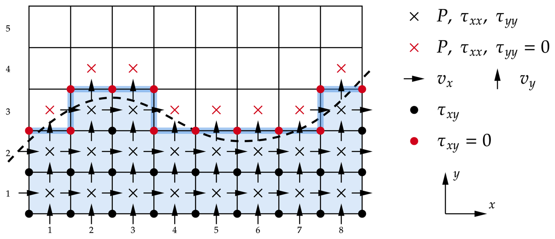
Figure 1 In the staircase method, cells are divided into rock (blue) and air (white). Between them is an interface, at which normal and shear stresses are set to zero in order to create free surface boundary conditions.

The staircase method comes with some limitations. The first limitation is one of accuracy. By imposing free surface boundary conditions at a staircase boundary between cells, it approximates the solution to the free surface problem. Unlike the sticky air method, which implicitly accounts for surface position at a sub-grid level through the viscosity field, the staircase method's discrete interface is less accurate, especially at coarser resolutions such as those used in global models.

While Duretz et al. (2016) did not demonstrate this issue explicitly, their study compared the staircase method to a similarly discretised sticky air method that also used a discrete viscosity jump between air and rock layers. When comparing the staircase method to a sticky air method with a smooth viscosity transition that accounts for the sub-grid location of the surface, the staircase method performs less favourably, introducing a systematic error that persists across all resolutions. These results can be seen in Sect. 5.1.

Another limitation of the staircase method is the absence of explicit velocity solutions above the surface. This creates challenges when using Lagrangian tracers near the surface, as velocity interpolation from the Eulerian grid requires contributions from neighbouring grid points. When air layer velocities are set to zero, inaccuracies arise in the advection of tracers near the surface.

A further limitation of the staircase method is that when using a multigrid solver, the location of the surface on the coarser grids may not match the location of the surface on the finer grid levels, which introduces some complexity to the restriction and prolongation operators, potentially reducing iteration convergence, as discussed after the test results.

3 Variational Stokes method

A discretisation of the Stokes equations on staggered grids that implicitly models free surface boundary conditions was proposed by Larionov et al. (2017), henceforth referred to as the variational method. The method is conceptually similar to the staircase method in that it does not involve the solution of any equations within the air layer, instead modelling the free surface boundary condition through the use of alternative boundary conditions at the interface. The two methods differ in how they implement these alternative boundary conditions. While the staircase method used a discrete staircase representation of the surface at cell boundaries, the variational method constructs a smooth representation of the free surface boundary condition at the interface by using volume fractions.

3.1 Variational form of the Stokes equations

The variational form of the Stokes equations considers the steady-state, incompressible Stokes equations with variables: velocity v, pressure p, deviatoric stress tensor τ, density ρ, and gravitational acceleration g. The continuity and momentum equations are, respectively:

$$\begin{array}{}\text{(2)}& \mathrm{\nabla }\cdot \mathit{v}=\mathrm{0},-\mathrm{\nabla }p+\mathrm{\nabla }\cdot \mathit{\tau }+\mathit{\rho }\mathbf{g}=\mathbf{0},\end{array}$$

where the deviatoric stress tensor τ is related to velocities by the constitutive law for an incompressible Newtonian viscous fluid:

$$\begin{array}{}\text{(3)}& \mathit{\tau }=\mathit{\eta }\left(\mathrm{\nabla }\mathit{v}+(\mathrm{\nabla }\mathit{v}{)}^{\mathrm{T}}\right).\end{array}$$

These equations can be reformulated in a variational form, where the problem is expressed as a functional for which a stationary point is sought in order to recover the original equations. Following Larionov et al. (2017), the variational formulation including body forces is given by:

$$\begin{array}{}\text{(4)}& \begin{array}{rl}\underset{p,\mathit{\tau }}{max}\underset{\mathit{v}}{min}\underset{{\mathrm{\Omega }}_{\mathrm{F}}}{\iiint }& -p\mathrm{\nabla }\cdot \mathit{v}+\mathit{\tau }:\left({\displaystyle \frac{\mathrm{\nabla }\mathit{v}+(\mathrm{\nabla }\mathit{v}{)}^{\mathrm{T}}}{\mathrm{2}}}\right)\\ & -{\displaystyle \frac{\mathrm{1}}{\mathrm{4}\mathit{\eta }}}|\mathit{\tau }{|}_F^{\mathrm{2}}-\mathit{\rho }\mathbf{g}\cdot \mathit{v}\mathrm{d}V.\end{array}\end{array}$$

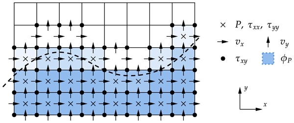
This continuous variational formulation may be discretised on a staggered grid following Larionov et al. (2017). The key step is to approximate the continuous volume integrals over the fluid domain Ω_F cellwise: each term in the integrand is evaluated at the discrete sample point of the relevant variable (cell centre for pressure, cell face for velocity, and cell centre or vertex for stress components), and the integral over that variable's control volume is approximated by multiplying the discretised term by the fractional volume of fluid material within that control volume. This fractional volume is the volume fraction ϕ, discussed further in Sect. 3.3. For cells entirely within the fluid domain ϕ=1 and the standard finite difference stencil is recovered exactly; for cells entirely outside the fluid ϕ=0 and those equations are excluded from the system; and for interfacial cells $\mathrm{0}<\mathit{\varphi }<\mathrm{1}$, giving a smooth approximation of the free surface boundary condition at sub-grid resolution. The discrete operators G, D, and M introduced below are therefore identical to those used in the standard staggered-grid Stokes discretisation – no new operators are required – and the entire effect of the free surface is encoded in the volume fraction weights that scale each term. The resulting discrete variational problem is:

$$\begin{array}{}\text{(5)}& \underset{p,\mathit{\tau }}{max}\underset{\mathit{v}}{min}{\mathbf{p}}^{\mathrm{T}}{\mathbf{G}}^{\mathrm{T}}\mathit{v}+{\mathit{\tau }}^{\mathrm{T}}\mathbf{D}\mathit{v}-{\displaystyle \frac{\mathrm{1}}{\mathrm{4}}}{\mathit{\tau }}^{\mathrm{T}}{\mathbf{M}}^{-\mathrm{1}}\mathit{\tau }-{\mathit{v}}^{\mathrm{T}}\mathit{\rho }\mathbf{g},\end{array}$$

where the continuous integrals of Eq. (4) have been replaced by their discrete analogues: the matrix G is the discrete gradient operator, with G^Tv representing the discrete divergence by the adjoint relationship between the two; D is the discrete symmetric gradient operator $\frac{\mathrm{1}}{\mathrm{2}}(\mathrm{\nabla }+{\mathrm{\nabla }}^{\mathrm{T}})$; and M is a diagonal matrix of viscosity coefficients at the stress locations corresponding to the structure of τ. The body force term v^Tρg is the discrete counterpart of the volume integral ${\iiint }_{{\mathrm{\Omega }}_{\mathrm{F}}}\mathit{\rho }\mathbf{g}\cdot \mathit{v}\mathrm{d}V$ in Eq. (4). Differentiating Eq. (5) with respect to v, τ, and p then recovers the discretised Stokes equations, which after stress elimination yield Eq. (8).

3.2 Stress elimination in the variational Stokes discretisation

Differentiating the discretised variational formulation with respect to velocity v, deviatoric stress τ, and pressure p produces the block system:

$$\begin{array}{}\text{(6)}& \left[\begin{array}{ccc}\mathrm{0}& {\mathbf{D}}^{\mathrm{T}}& \mathbf{G}\\ \mathbf{D}& -\frac{\mathrm{1}}{\mathrm{2}}{\mathbf{M}}^{-\mathrm{1}}& \mathrm{0}\\ {\mathbf{G}}^{\mathrm{T}}& \mathrm{0}& \mathrm{0}\end{array}\right]\left[\begin{array}{c}\mathit{v}\\ \mathit{\tau }\\ \mathbf{p}\end{array}\right]=\left[\begin{array}{c}\mathit{\rho }\mathbf{g}\\ \mathrm{0}\\ \mathrm{0}\end{array}\right].\end{array}$$

Rearranging the central row gives the constitutive relation:

$$\begin{array}{}\text{(7)}& \mathit{\tau }=\mathrm{2}\mathbf{MD}\mathit{v},\end{array}$$

which can be substituted into the remaining rows to eliminate τ, yielding the discretised Stokes equations:

$$\begin{array}{}\text{(8)}& \left[\begin{array}{cc}\mathrm{2}{\mathbf{D}}^{\mathrm{T}}\mathbf{MD}& \mathbf{G}\\ {\mathbf{G}}^{\mathrm{T}}& \mathrm{0}\end{array}\right]\left[\begin{array}{c}\mathit{v}\\ \mathbf{p}\end{array}\right]=\left[\begin{array}{c}\mathit{\rho }\mathbf{g}\\ \mathrm{0}\end{array}\right],\end{array}$$

where G is the discrete gradient operator (with G^T the discrete divergence), D is the discrete symmetric gradient operator $\frac{\mathrm{1}}{\mathrm{2}}(\mathrm{\nabla }+{\mathrm{\nabla }}^{\mathrm{T}})$, and M is a diagonal matrix of viscosity coefficients at the stress locations. With appropriate discrete operators G and D, this recovers an identical set of equations to the velocity-pressure Stokes system solved by StagYY and many other geodynamic codes. Where prescribed traction boundary conditions are required at the free surface, for instance when an external load is not explicitly modelled by the Stokes solver, an additional right-hand side contribution can be derived from the energy required to push against a surface stress field ${\mathit{\sigma }}_{\text{BC}}=p_{\text{BC}}\mathbf{I}-{\mathit{\tau }}_{\text{BC}}$. Applying the divergence theorem over the air portion of the domain Ω_A and introducing the air fraction $\mathit{\xi }=\mathrm{1}-\mathit{\varphi }$, the discretised traction contribution to the right-hand side is:

$$\begin{array}{}\text{(9)}& \left[\begin{array}{c}\mathbf{G}{\mathit{\xi }}^p{p}_{\text{BC}}-{\mathit{\xi }}^v\mathbf{G}{p}_{\text{BC}}+{\mathbf{D}}^{\mathrm{T}}{\mathit{\xi }}^{\mathit{\tau }}{\mathit{\tau }}_{\text{BC}}-{\mathit{\xi }}^v{\mathbf{D}}^{\mathrm{T}}{\mathit{\tau }}_{\text{BC}}\\ \mathrm{0}\end{array}\right],\end{array}$$

which is simply added to the right-hand side of Eq. (8). This contribution is nonzero only within interfacial cells where the appropriate volume fractions and air fractions are simultaneously nonzero.

3.3 Volume fractions

Further progress on the free surface problem requires the use of cellwise volume fractions. The volume fraction function, denoted by ϕ, is defined as the fraction of material (rock, for geodynamic applications) occupying a given computational cell, and therefore satisfies ϕ=0 for a completely empty cell and ϕ=1 for a completely full cell (Fig. 2). Partially filled cells arise in the vicinity of the free surface.

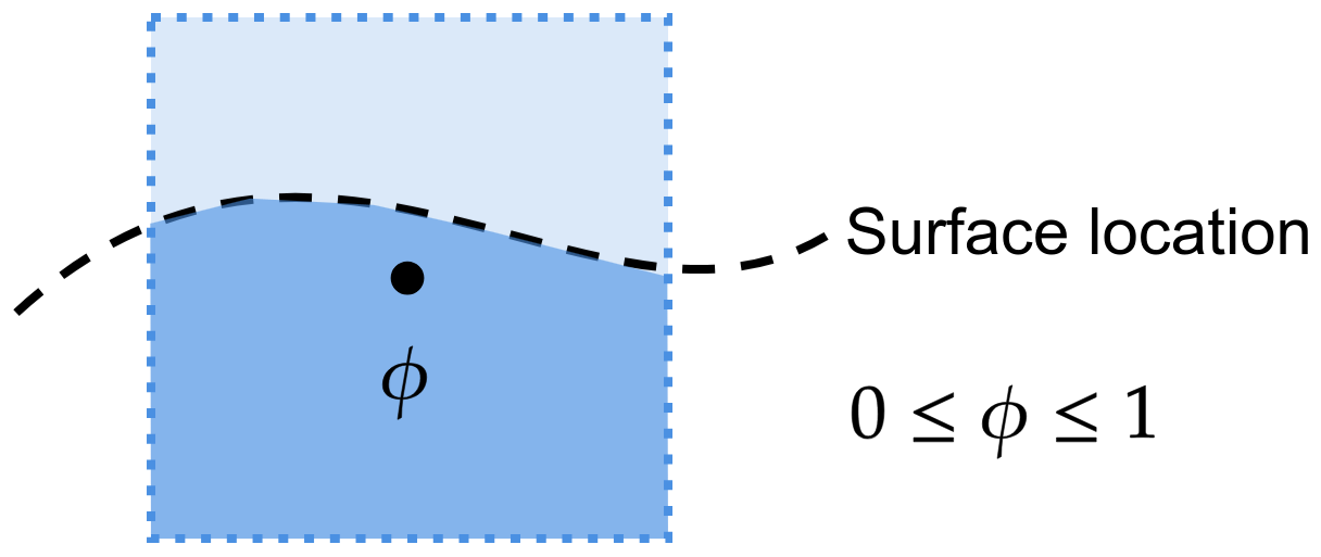
Figure 2 The volume fraction function ϕ for a given control volume is defined as 0 if the cell is completely empty, and 1 if it is completely full.

On a staggered grid, variables are located at cell centres, faces, edges, and nodes. Volume fractions are therefore defined at the corresponding locations: ϕ^P for pressure points (cell centres), and ϕ^τ for stresses, which may be located at cell vertices or cell centres. For example, ${\mathit{\varphi }}^{{\mathit{\tau }}_{xx}}$ and ${\mathit{\varphi }}^{{\mathit{\tau }}_{yy}}$ are located at cell centres and are identical to ϕ^P, while ${\mathit{\varphi }}^{{\mathit{\tau }}_{xy}}$ is located at cell vertices in 2D (edge centres in 3D).

A key result of Larionov et al. (2017) is that the free surface problem can be treated by multiplying the terms in the discretised variational formulation by their corresponding volume fractions, motivated by the fact that the continuous volume integrals over Ω_F are approximated cellwise using ϕ. Applying this to Eq. (8) yields the full free-surface pressure-velocity system:

$$\begin{array}{}\text{(10)}& \left[\begin{array}{cc}\mathrm{2}{\mathbf{D}}^{\mathrm{T}}\mathbf{M}{\mathit{\varphi }}^{\mathit{\tau }}\mathbf{D}& \mathbf{G}{\mathit{\varphi }}^{\mathrm{P}}\\ {\mathit{\varphi }}^{\mathrm{P}}{\mathbf{G}}^{\mathrm{T}}& \mathrm{0}\end{array}\right]\left[\begin{array}{c}\mathit{v}\\ \mathbf{p}\end{array}\right]=\left[\begin{array}{c}{\mathit{\varphi }}^{{\mathrm{v}}_z}\mathit{\rho }\mathbf{g}\\ \mathrm{0}\end{array}\right],\end{array}$$

where ${\mathit{\varphi }}^{{\mathrm{v}}_z}$ is the volume fraction evaluated at vertical velocity points, and ρ is the density field evaluated at the same locations. For consistency with the volume-fraction weighting of the left-hand side, the density is taken as the product of a background density and the appropriate volume fraction, so that the body force vanishes automatically in cells outside the fluid domain. This approach introduces minor errors near lateral density variations, discussed further in Sect. 4.2.

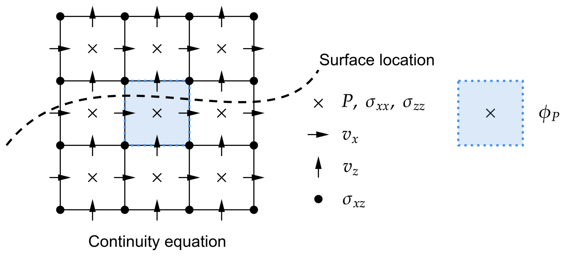
Figure 3 The continuity equation is solved in a given cell if the volume fraction centred on the central pressure point is nonzero, i.e. ϕ_P>0.

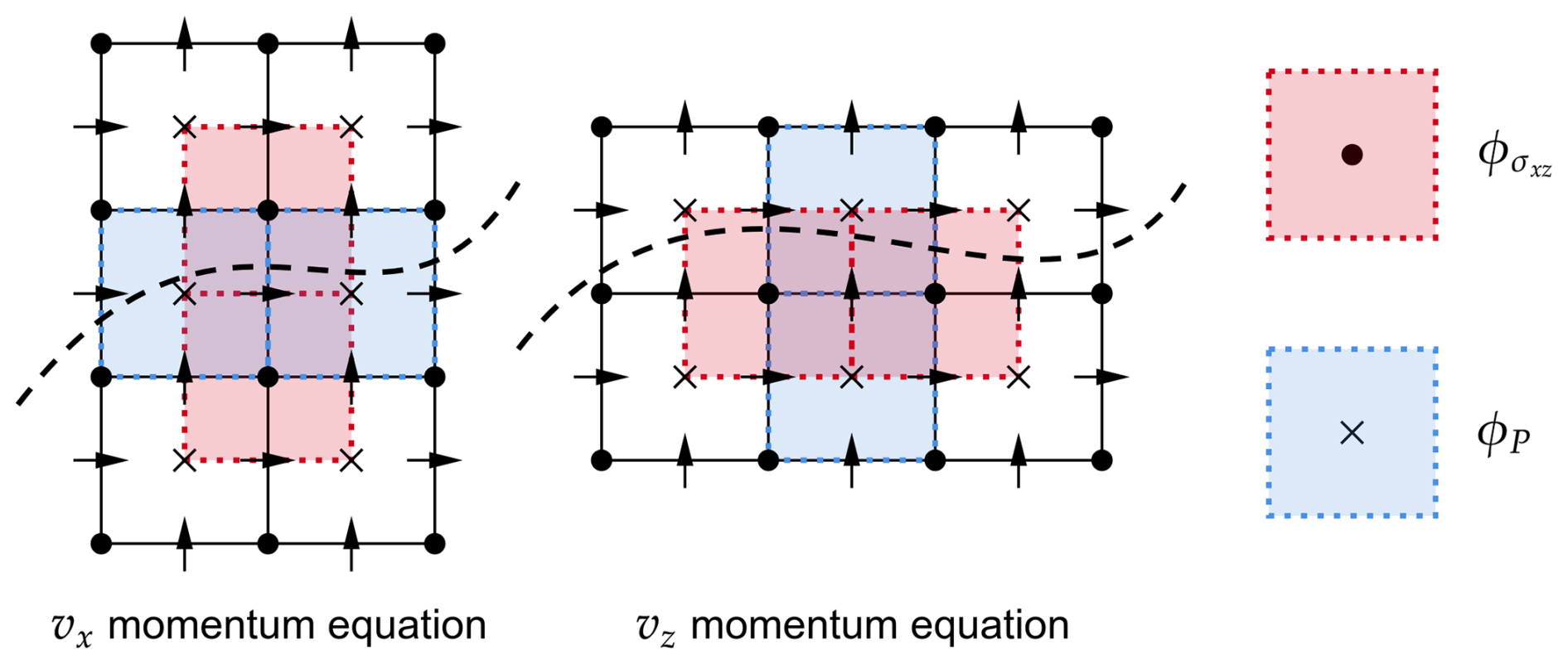
Figure 4 In 2D, the v_x and v_z momentum equations are solved only if at least one of the pictured volume fractions surrounding the velocity point is nonzero.

Since ϕ^P=0 for cells entirely outside the fluid domain, the discretised continuity equation ϕ^PG^Tv=0 is solved only where fluid is present. Likewise, momentum equations are omitted where both ϕ^τ and ϕ^P are simultaneously zero. In these cases the system becomes singular, and the corresponding pressure or velocity degrees of freedom are set to zero. The control volumes governing equation activation in 2D are illustrated in Figs. 3 and 4.

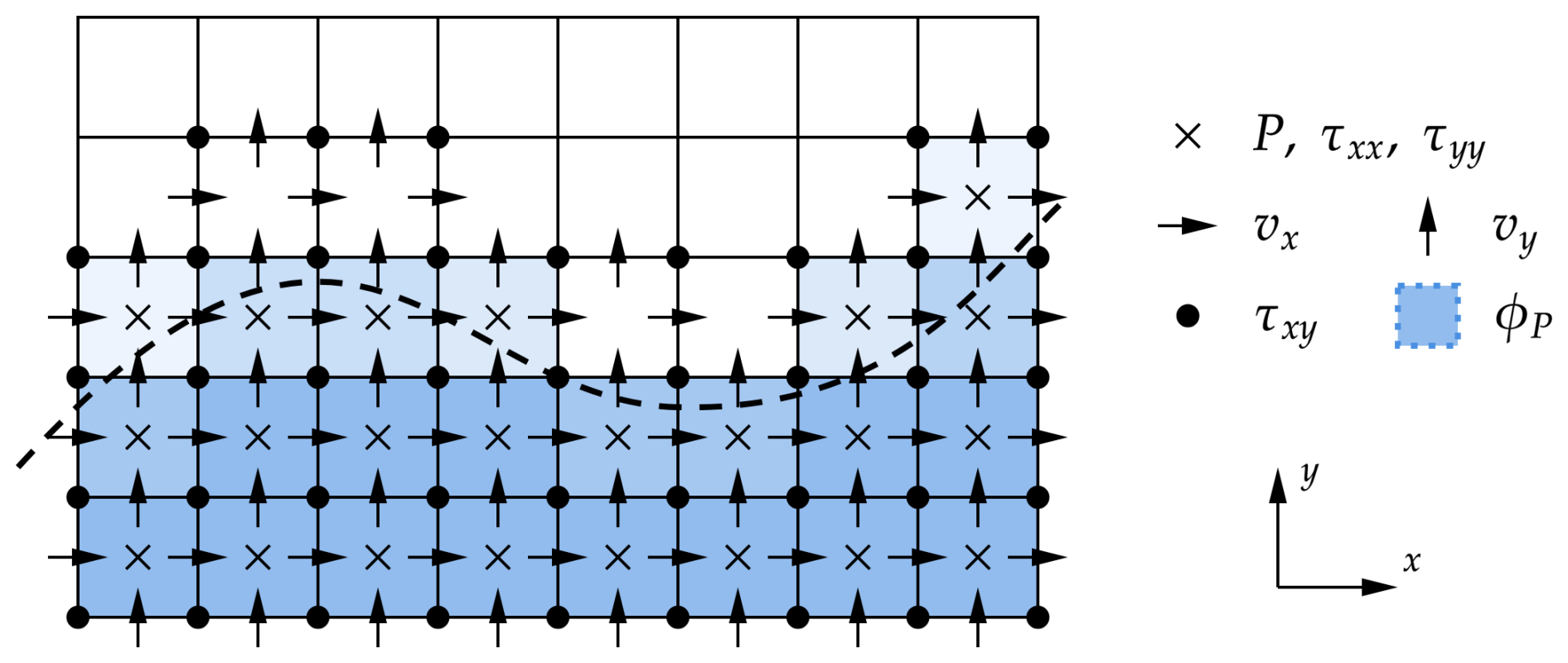
Figure 5 The discretised Stokes equations on a simplified domain using the variational method. Cell-centred volume fractions ϕ_P dictate where the continuity equation is solved; cells with zero volume fraction (white) are excluded.

The result is a system that excludes pressure unknowns in cells with no fluid content and excludes velocity unknowns more than 1.5 cell widths from the surface. A benefit over the staircase method is that velocities are explicitly computed within 1.5 cell distances of the surface, making direct interpolation of surface velocities possible without extrapolation. The discretisation for the same domain shown in Fig. 1 is illustrated for the variational method in Fig. 5.

4 Implementation using staggered-grid finite differences

The implementation of the variational Stokes method in a finite-difference numerical geodynamical modelling code such as StagYY involves several steps: determination of volume fractions, the treatment of boundary conditions, the treatment of near-surface densities and viscosities, and the application of the method to the multigrid solver.

4.1 Obtaining volume fractions

Volume fractions ϕ are a prerequisite for implementing the variational Stokes method. There are several possible methods for obtaining volume fractions, such as Lagrangian surface tracking or the volume of fluid method (Gray et al., 2026a, b). In this study, Lagrangian surface tracking was used exclusively to track the surface.

When using a Lagrangian tracking method to track the location of the surface, such as the surface marker chain or mesh, it is possible to obtain the volume fractions required for the variational method by integrating underneath the surface. In 2D, volume fractions may be determined by iterating over the piecewise linear representation of the surface, and determining whether each given cell is fully beneath the surface, fully above, or partially below and above. In all cases tested, the computational effort required to obtain volume fractions scales linearly O(n) with number of surface markers, and computational cost of determining them was experimentally found to be small in comparison to the total runtime of the models (Gray et al., 2026a).

4.2 Near-surface densities and viscosities

In order to capture near-surface densities and viscosities, a reference value must be chosen for density and viscosity near the surface, to which the appropriate volume fraction is multiplied in order to obtain a fractional value. This approach works for situations in which density and viscosity are constant, as the reference values are known. However, in situations where there are lateral hetereogeneities in near-surface density and viscosity, it can result in minor errors as the reference values may not correspond to the actual density near-surface values at all points.

A potential solution to this problem is to copy reference values from cells immediately below the surface, i.e. the closest cell that does not contain air. In testing, while this approach appeared to provide more accurate results for the density field, testing with the 2D subduction benchmark presented by Schmeling et al. (2008) resulted in differing subduction behaviour as a consequence of subtle variations in the viscosity field near the air-mantle-slab triple junction. In some cases due to the copying of these viscosities, slab break-off was made impossible as it became impossible to create a mantle wedge. As a consequence of this negative result, the results shown consider the use of fixed reference densities and viscosities. Finding the correct treatment for near-surface viscosities is a key future research direction.

Volume fraction restriction to coarse grids when using the multigrid method

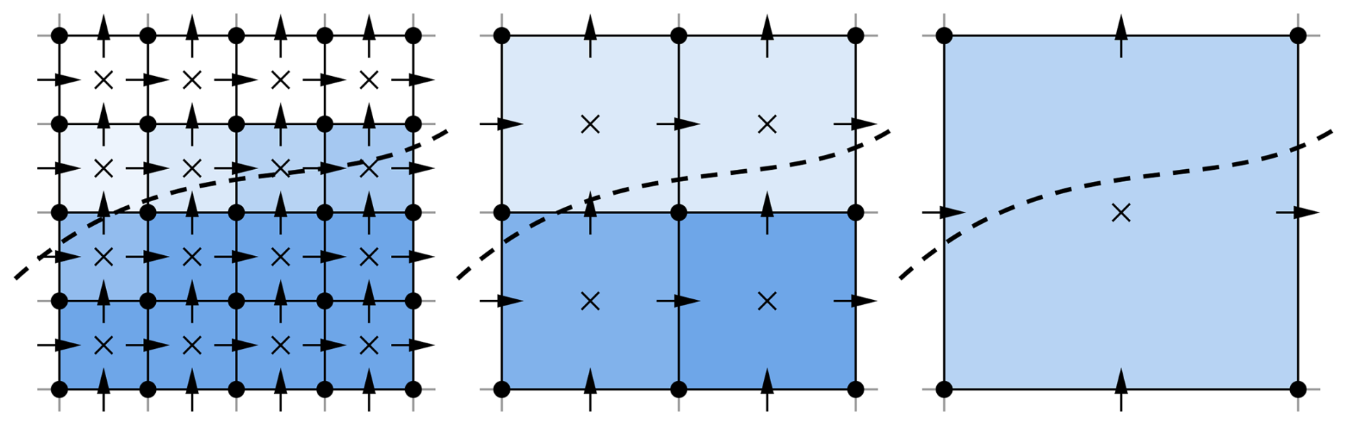
Figure 6 Restriction of the volume fraction function can be achieved by combining neighbouring volume fractions on the fine grid to form the coarse grid.

4.3 Multigrid solver

A key feature of the variational Stokes method is its ability to be applied to multigrid solvers. The application of volume fraction based methods to multigrid solvers has been demonstrated in the past. For example, Rauwoens et al. (2015) demonstrated the use of a volume fraction based on the solver developed by (Botto, 2013) for solving Poisson equations with a multigrid solver.

The multigrid implementation can be achieved by restricting the volume fraction field to a coarse grid through simple averaging of fine grid volume fractions (Fig. 6). In contrast, in the staircase method the volume fraction is either 1 or 0.

This coarse grid restriction can easily be achieved in 2D and 3D by averaging 4 or 8 fine grid cells, respectively. The extension to 3D is particularly important, as 3D models in StagYY require the use of iterative multigrid solvers.

5 Test results

Results are demonstrated in both 2D and 3D for the three free surface modelling methods: the sticky air method, staircase method, and the newly implemented variational method. These benchmarks aim to demonstrate the accuracy and efficiency of the new variational method in comparison to the existing free surface modelling methods.

Unless stated otherwise, the surface is tracked for all methods using Lagrangian surface tracking with a bilinear interpolation step, similar to that described in Duretz et al. (2016). This method was found to be able to accurately track free surfaces with minimal additional computational cost.

5.1 2D inclusion benchmark

Analytical solutions to simple problems involving the Stokes equation exist for benchmarking our methods. An analytical solution was employed by Duretz et al. (2016) to benchmark the staircase method and examine its performance when scaling with resolution.

The test involves Stokes flow around a viscous inclusion in a 2D Cartesian domain, for which there exists an analytical solution (Schmid and Podladchikov, 2003). In the case of a vanishing inclusion viscosity, the boundary conditions at the interface are identical to free surface boundary conditions (i.e. zero normal and shear stress at the interface). Dirichlet boundary conditions are imposed at the other edges of the model, which correspond to the analytical solution. This test was implemented in code written in Julia, based on the original MATLAB version presented in Duretz et al. (2016).

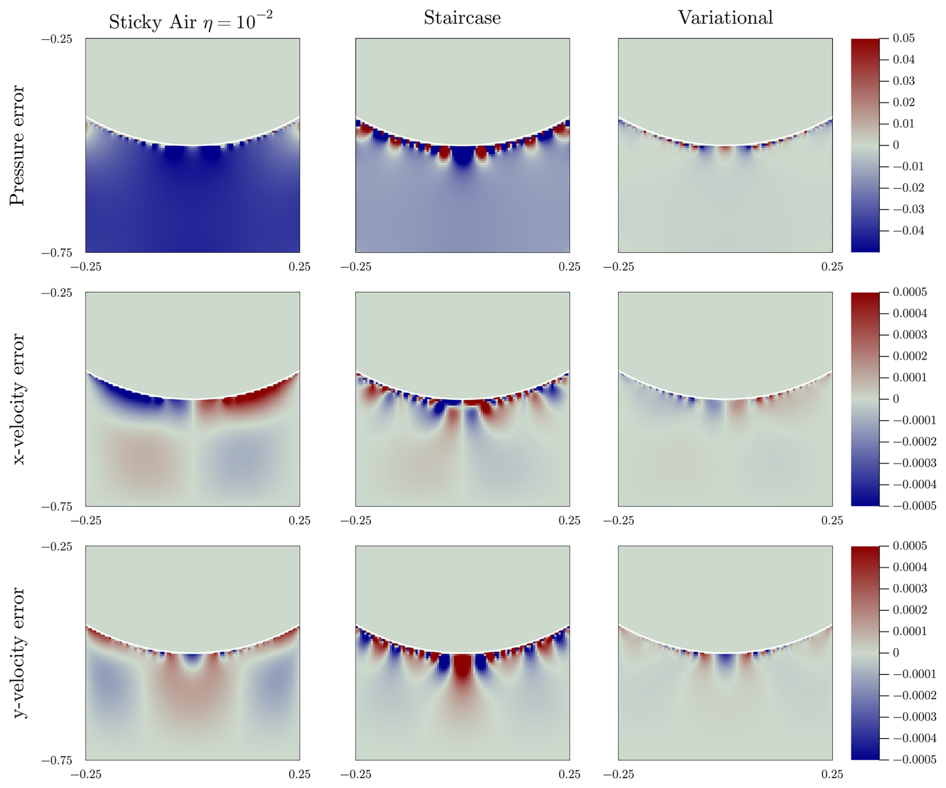
Figure 7 Errors in pressure (top row), x-velocity (middle row), and y-velocity (bottom row) for the sticky air method with ${\mathit{\eta }}_{\text{rock}}/{\mathit{\eta }}_{\text{air}}={\mathrm{10}}^{\mathrm{2}}$ (left column), the staircase method (centre column), and the variational method (right column), each run at a resolution of 100 × 100. The sticky air method produces significant errors at and near the interface; these near-boundary errors are caused by the viscosity discontinuity itself and persist regardless of the viscosity contrast (Deubelbeiss and Kaus, 2008; Heister et al., 2017). The staircase method reduces far-field errors but exhibits elevated errors near the surface owing to its discrete boundary representation. The variational method achieves the closest agreement with the analytical solution, reducing both near- and far-field errors across all fields.

An improved version of the sticky-air method was implemented, differing from the results presented in (Duretz et al., 2016). The results of that paper considered viscosity as a step function, where a cell whose midpoint was below the surface had the rock viscosity, and the cells whose midpoint was above had the air viscosity. This resulted in an unrealistic representation of viscosity, especially compared to how viscosity is typically computed in numerical geodynamic models. In these results, viscosity near the surface is multiplied with the appropriate volume fraction in order to obtain a smooth representation of viscosity near the surface, providing more accurate sticky air results than the original paper. This approach also highlights the limitations of the staircase discretisation arising from a discrete staircase representation of the surface.

The three surface modelling methods are compared against the analytical solution in terms of pressure and velocity errors. Figure 7 shows the absolute errors of the sticky air method (with ${\mathit{\eta }}_{\text{rock}}/{\mathit{\eta }}_{\text{air}}={\mathrm{10}}^{\mathrm{2}}$), the staircase method, and the variational method with respect to the analytical solution when run with a model resolution of 100 × 100. Only cells entirely within the fluid domain are compared, as cells within the air layer do not correspond to physical values for this case.

The results qualitatively show that the variational method reduces errors in solution in comparison to both the sticky air method and the staircase method. The difference is most apparent when considering the pressure error. The sticky air method, as a result of its large viscosity contrast that cuts across grid cells, produces large errors in pressure at the boundary (Deubelbeiss and Kaus, 2008; Heister et al., 2017) and an offset throughout the domain. While the staircase method is able to reduce the error far from the surface, this comes at the cost of high errors close to the surface arising from the discrete nature of the staircase approach. The variational method appears to be able to overcome many of these near- and far-field errors, and provide a visibly closer fit to the analytical solution overall. A similar situation exists for the velocity errors.

In order to quantitatively analyse the performance of each method, models were run at a range of resolutions ranging from 10 × 10 to 1200 × 1200 cells. The errors in pressure and velocities using the L₁ norm can then be compared and plotted as a function of grid spacing to investigate the scaling performance of each method. As the sticky air method is viscosity dependent, three viscosity contrasts were compared, namely ${\mathit{\eta }}_{\text{air}}/{\mathit{\eta }}_{\text{rock}}={\mathrm{10}}^{-\mathrm{3}}$, 5 × 10⁻³, and 10⁻².

Figure 8 considers the pressure errors in the L₁ norm over the i cells in the model. The definition of these errors is given by:

$$\begin{array}{}\text{(11)}& \left|\right|P-P_{\mathrm{a}}|{|}_{L_{\mathrm{1}}}={\displaystyle \frac{\mathrm{1}}{V}}\sum _{i\in \mathrm{\Omega }}|P_i-P_{i,\mathrm{a}}|.\end{array}$$

where Ω denotes the fluid domain, V is the volume of the fluid domain, and P_a is the analytical solution.

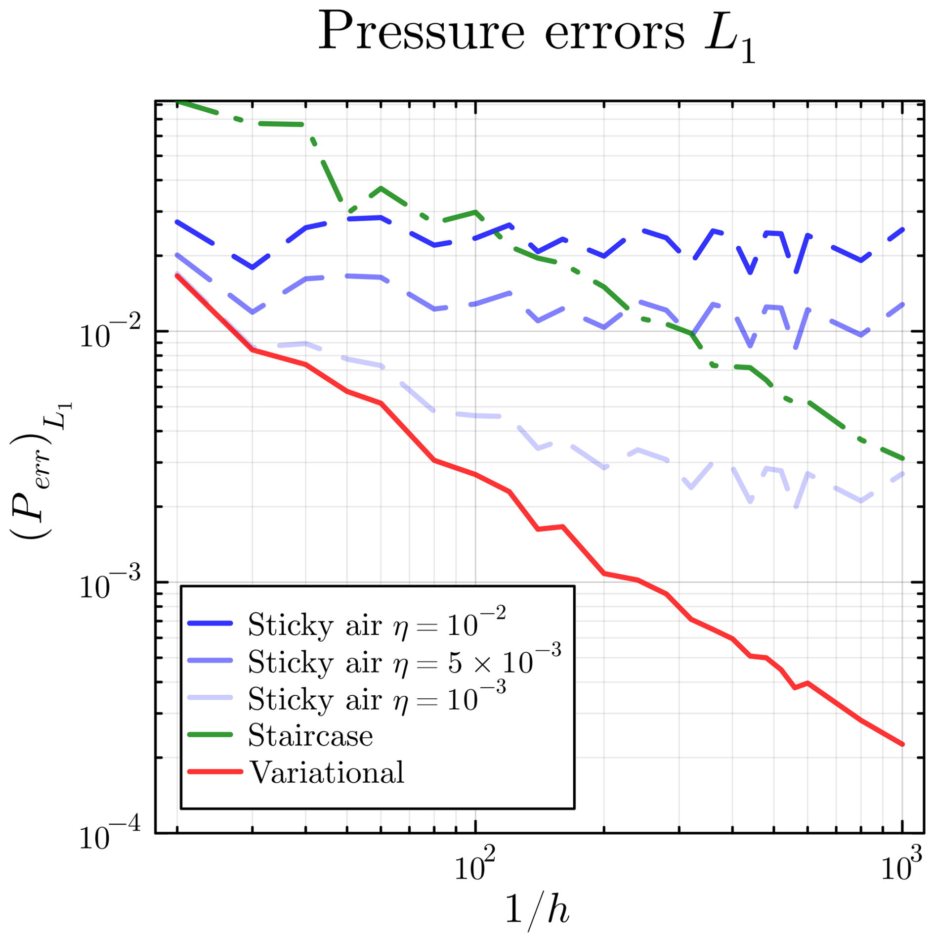
Figure 8 The L₁ error in pressure P_err follows a first order scaling with increasing grid resolution $\mathrm{1}/h$. The sticky air method quickly fails depending on viscosity, and the staircase method also achieves first order scaling but is overall less accurate.

These pressure error tests reveal that the pressure errors with the variational method have first order scaling with resolution in the L₁ norm, similarly to the staircase method.

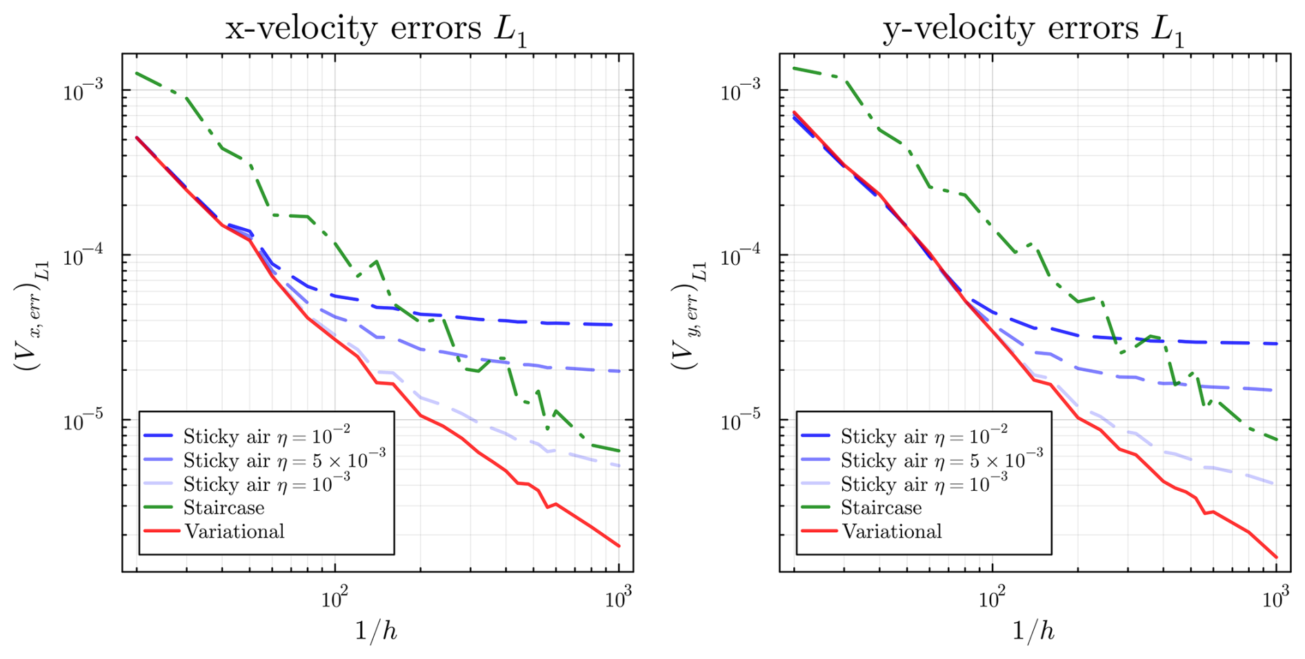
Figure 9 The L₁ error in velocity for the variational method achieves first order scaling with grid spacing, as does the staircase method. The scaling of the sticky air method is viscosity contrast dependent. The variational method is overall more accurate than the staircase method.

In Fig. 9, the errors in velocity in each dimension are compared using the L₁ norm, with definitions similar to those of the pressure errors.

The results from this analytical test reveal that the variational Stokes method is overall more accurate than the staircase method, and does not suffer from the viscosity contrast dependence of the sticky air method which becomes apparent at higher resolution.

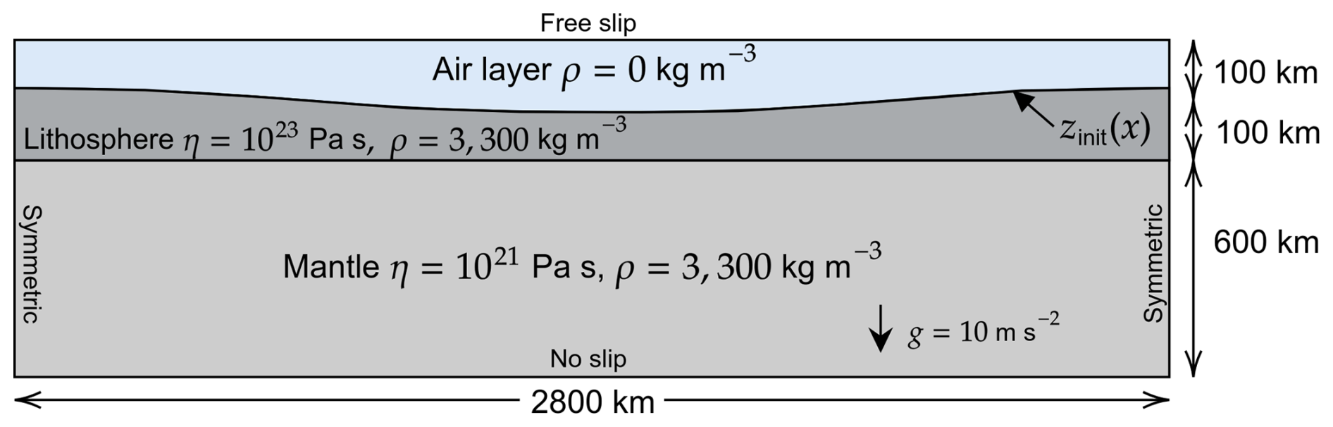
Figure 10 2D surface relaxation benchmark based on Case 1 presented by Crameri et al. (2012). An initially non-flat surface in a three-layer model relaxes until equilibrium is reached after approximately 100 ky.

5.2 2D relaxation benchmark

The 2D surface relaxation benchmark (Fig. 10) is based on Case 1 as presented by Crameri et al. (2012). It considers the time dependent relaxation of an initially non-flat surface with initial topography z_init(x) given by the function:

$$\begin{array}{}\text{(12)}& z_{\text{init}}\left(x\right)=\mathrm{7}\cos \left({\displaystyle \frac{\mathrm{2}\mathit{\pi }x}{\mathrm{2800}\mathrm{km}}}\right)\mathrm{km}.\end{array}$$

The model domain is a 2800 km × 800 km Cartesian box consisting of three compositional layers: a 600 km thick mantle layer, a more viscous 100 km thick lithosphere, and a 100 km thick air layer. This problem is simple enough to have an analytical solution for surface position as a function of time as derived using a three-layer model (Ramberg, 1981). Starting from an initial maximum of 7 km, the maximum topography as a function of time z max(t) is given by:

$$\begin{array}{}\text{(13)}& z_{\text{max}}\left(t\right)=\mathrm{7}\exp \left({\displaystyle \frac{-t}{\mathrm{14.825}\mathrm{y}}}\right)\mathrm{km}.\end{array}$$

In the tests here the resolution is 512 × 128, with 100 tracers per cell for advecting material properties. When using the sticky air method, a viscosity of 10¹⁸ Pa s was used. Symmetric boundary conditions are imposed at the horizontal edges of the model, while a no-slip boundary condition is imposed at the bottom boundary, and a free slip condition is imposed at the top. Acceleration due to gravity g is set to 10 m s⁻². For consistency with the benchmarks run by Crameri et al. (2012), models were run until t = 100 ky to show the system reaching equilibrium. Timesteps were limited to 500 years in order to give high temporal resolution for plots of model evolution.

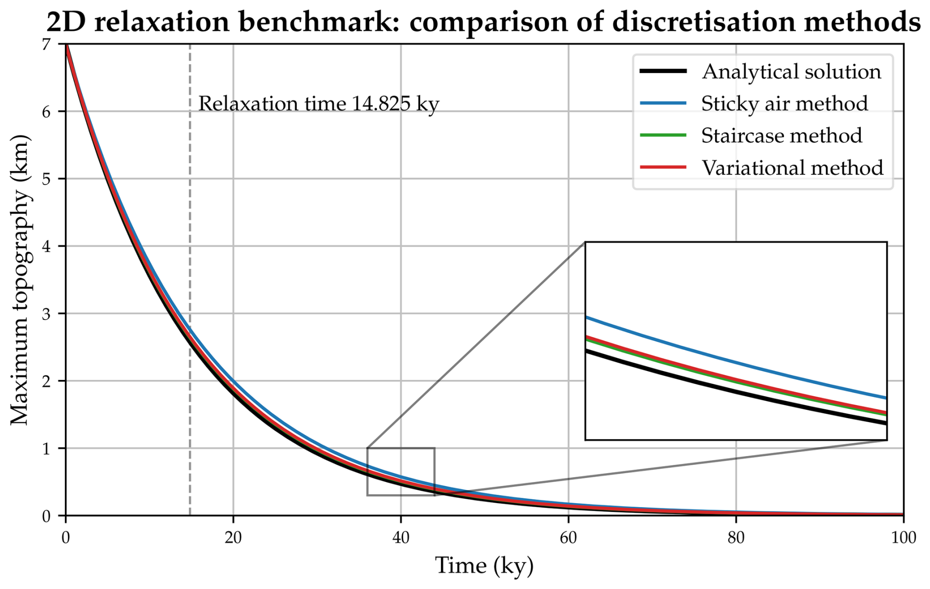
Figure 11 2D relaxation benchmark comparing performance of different discretisation methods with an analytical solution. All methods tested are able to closely track the analytical solution.

In Fig. 11, the three discretisation methods are compared against the analytical solution. The result of this benchmark shows that all methods are able to very closely track the analytical solution. The staircase and variational methods in particular are close to the analytical solution, perhaps as a result of minor surface stresses created by the interface to the sticky air layer preventing the sticky air method from relaxing as quickly.

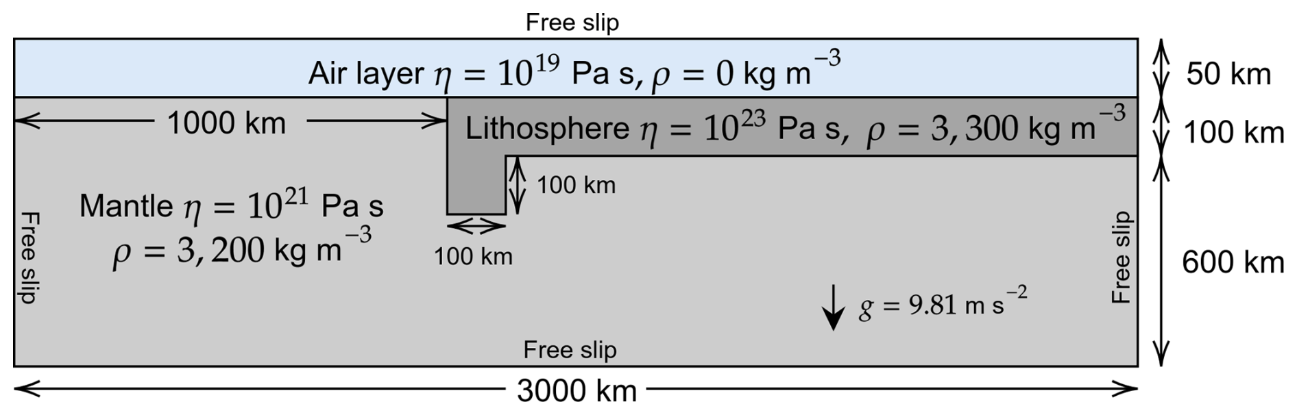
Figure 12 The 2D subduction benchmark is based on Case 1 presented in Schmeling et al. (2008), and considers subduction initiation in this simplified viscous setup. Diagram not to scale.

5.3 2D subduction benchmark

In order to test the ability of the implemented methods to track surfaces near convergent margins, particularly subduction zones, the simple isothermal viscous subduction benchmark proposed by Schmeling et al. (2008) was used with the model setup given in Fig. 12.

The model setup consists of a gravitationally unstable lithospheric slab sinking and initiating a new subduction zone. The models are run on a 3000 km × 750 km Cartesian box domain at a resolution of 512 × 64. The lithosphere has a thickness of 100 km, a density 100 kg m⁻³ greater than the surrounding mantle, and a viscosity 100 times greater than the surrounding mantle. At the top of the model is a 50 km thick air layer. When using the sticky air method, a viscosity of 10¹⁹ Pa s, 100 times lower than the viscosity of the mantle and 10 000 times lower than the viscosity of the slab, is used. Free slip boundary conditions are imposed on model boundaries. Acceleration due to gravity g is set to 9.81 m s⁻². The models were run for a total of 100 My.

The results for this benchmark presented in Schmeling et al. (2008) are notable for the large differences in results produced as a result of relatively minor changes in the viscosity field, such as the use of different viscosity interpolation schemes. This fundamental instability is a result of minute differences in viscosity near the mantle-lithosphere-air triple junction causing radically different subduction initiation behaviour. In the models run for this study, a geometric average is used for viscosity interpolation.

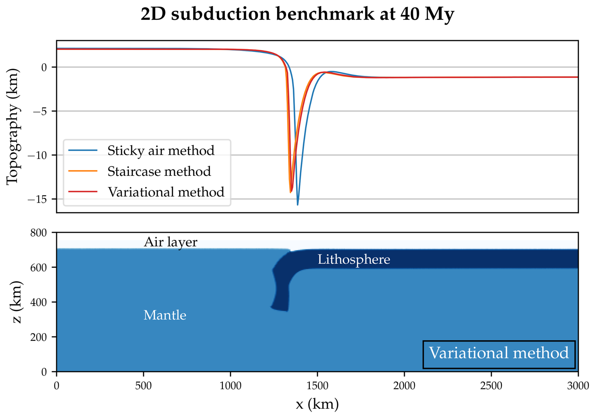
Figure 13 2D subduction benchmark topography after 40 My for the three discretisation methods. There are slight differences in subduction performance when using a sticky air method as opposed to either the staircase or variational methods, which produce very similar results.

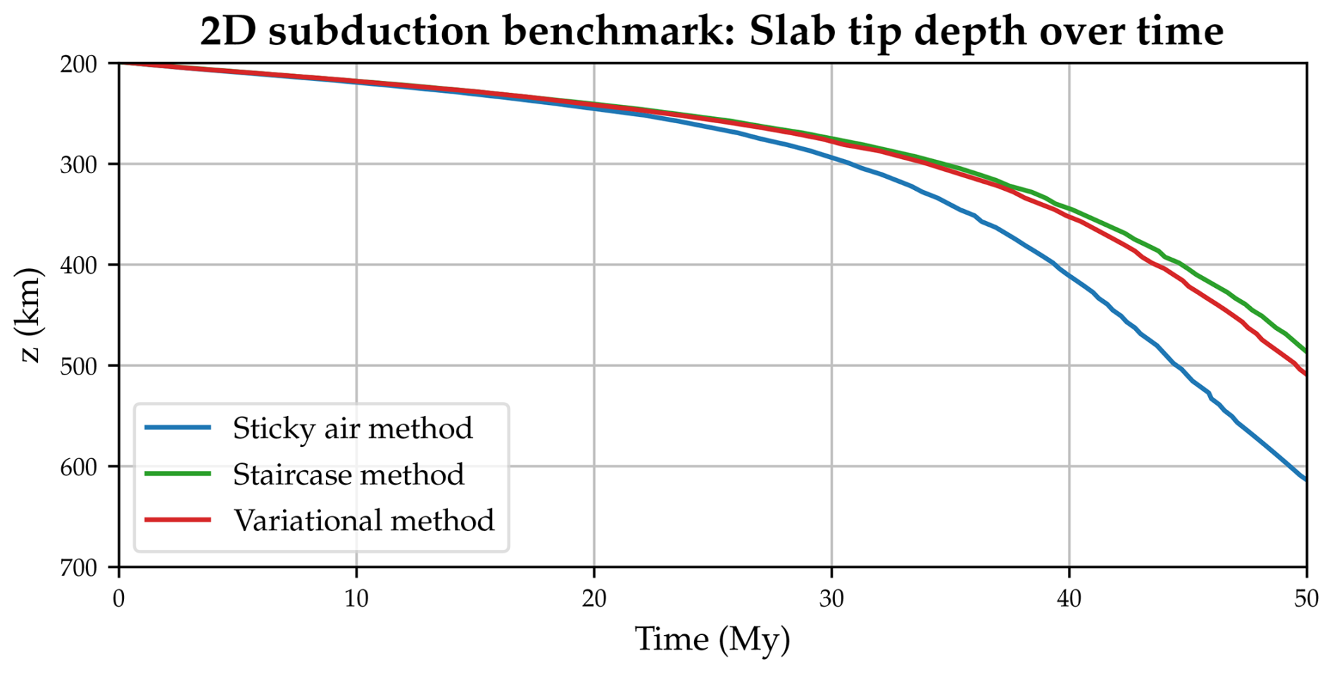
Figure 14 Slab tip depth over time for the three discretisation methods, demonstrating the slightly delayed subduction initiation seen when using the staircase and variational methods compared to the sticky air method.

The topography generated by the three methods, plotted at 40 My in Fig. 13, reveals that the variational method and staircase method produce extremely similar results, in contrast to the sticky air method, which exhibits slightly faster subduction; the corresponding slab profiles at 40 My are visually indistinguishable between the staircase and variational methods, with only a slightly more developed slab visible in the sticky air case. Figure 14 demonstrates the differing rates of subduction between the three methods by considering the depth of the tip of the subducting slab over time.

These results are not consistent with results obtained from the sticky air method with a higher viscosity contrast, in which case subduction was shown to be faster. While the two true free surface methods would be expected to show the fastest subduction due to a lack of resistance from the air layer, they instead produce slightly slower, delayed subduction. This behaviour is a direct consequence of the near-surface viscosity limitation described in Sect. 4.2: errors in the treatment of viscosity at interfacial cells affect the stress state near the air-mantle-lithosphere triple junction, which in turn influences subduction initiation timing. As noted there, this sensitivity is not specific to the variational method – Schmeling et al. (2008) document the same instability across a range of codes – but it does highlight that improving near-surface viscosity treatment is a prerequisite for reliable use of any free-surface method in subduction settings. This remains an important direction for future work, as discussed further in Sect. 6.

5.4 2D scaling tests

Scaling tests in 2D were performed using a non-dimensional model in spherical annulus geometry (Hernlund and Tackley, 2008). The model setup involves a constant viscosity mantle with Rayleigh number Ra=10⁷, an air layer with a thickness 10 % of the mantle's thickness, and, in the case of the sticky air method, a viscosity contrast of ${\mathit{\eta }}_{\text{rock}}/{\mathit{\eta }}_{\text{air}}={\mathrm{10}}^{\mathrm{3}}$. Each scaling model was run for 5000 timesteps to ensure steady-state convection was achieved. The computational performance of the Stokes solver–typically the most resource-intensive component of numerical geodynamic models–was assessed across three discretisation methods. Tests were conducted at various resolutions, ranging from 128 × 16 to 1024 × 128 to evaluate solver performance at different resolutions. Simulations were run in parallel on 4 cores for lower resolutions and 8 cores for higher resolutions, using an AMD Ryzen 9 3900XT processor.

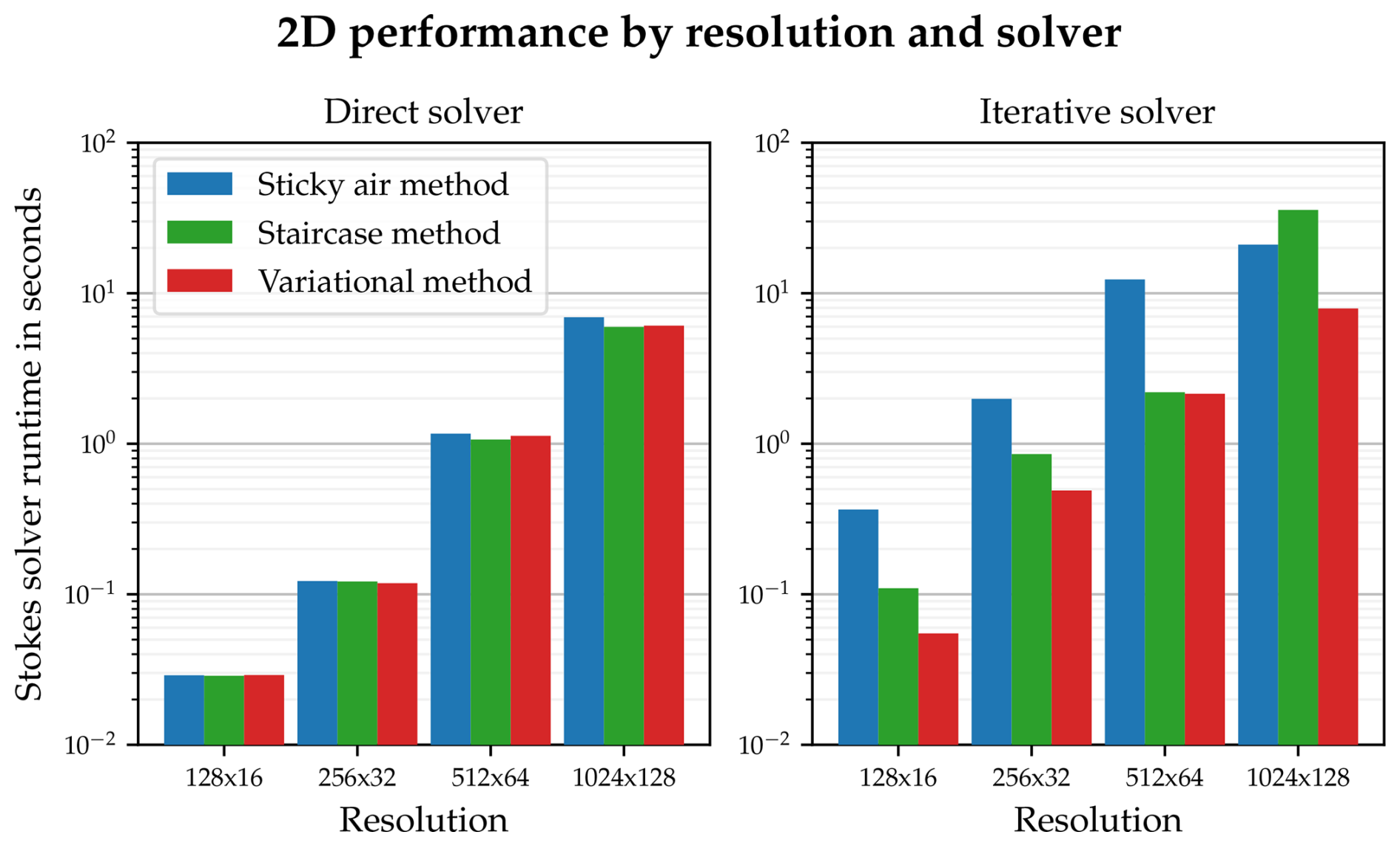
Figure 15 Mean Stokes solver runtime per timestep across all resolutions, comparing direct and iterative solvers. Performance is consistent between discretisation methods when using a direct solver (typical for 2D models), but with an iterative multigrid solver, significant performance gains are observed when using the variational method.

The performance results, illustrated in Fig. 15, show the mean Stokes solver runtime per timestep, averaged over 5000 timesteps. All methods perform comparably when using a direct solver–the most common approach for 2D models. For these tests the MUMPS solver (Amestoy et al., 2001, 2019) is used via the PETSc toolkit (Balay et al., 2025). This consistency aligns with the fact that the size of the linear system remains identical across discretisation methods. However, when employing an iterative multigrid solver, significant performance improvements are achieved with the staircase and variational methods, the latter offering the most notable and consistent gains over the sticky air method. This reflects a smaller number of multigrid V-cycles necessary to reach satisfactory convergence.

Interestingly, at the highest resolution of 1024 × 128, the staircase method exhibited worse performance than the sticky air method. This outcome, verified through repeated simulations, may indicate that this combination of resolution and free surface position is particularly challenging to solve. Such behaviour can conceivably arise when the position of the free surface at coarse grid levels does not match its position on the fine grid, reducing the effectiveness of coarse-grid iterations and necessitating more fine-grid iterations. Indeed, experiments indicate that the convergence of V-cycles can be quite sensitive to the vertical position of the free surface, supporting this interpretation. This problem does not appear to affect the variational method, which is able to approximate the free surface boundary condition with sub-grid resolution on coarse grids as well as on fine grids. On coarse grids the free surface remains in the same position, just becoming vertically smeared. It is possible that for the staircase method, more work on restriction and prolongation operators in the region of the free surface could improve convergence.

5.5 3D scaling tests

3D scaling tests are used to assess the performance of the three methods. A constant viscosity Cartesian box setup featuring convection with a Rayleigh number of Ra=10⁷ was run at a variety of resolutions ranging from 32 × 32 × 16 to 256 × 256 × 128. When using the sticky air method, an air layer with viscosity 1000 times less than the mantle and 10 % the thickness of the mantle was used. Models were run for a total of 5000 timesteps to ensure a steady state convection was reached. As direct solvers are unavailable for 3D cases, only iterative multigrid solvers can be compared, in contrast with the 2D performance benchmarks shown in Sect. 5.4.

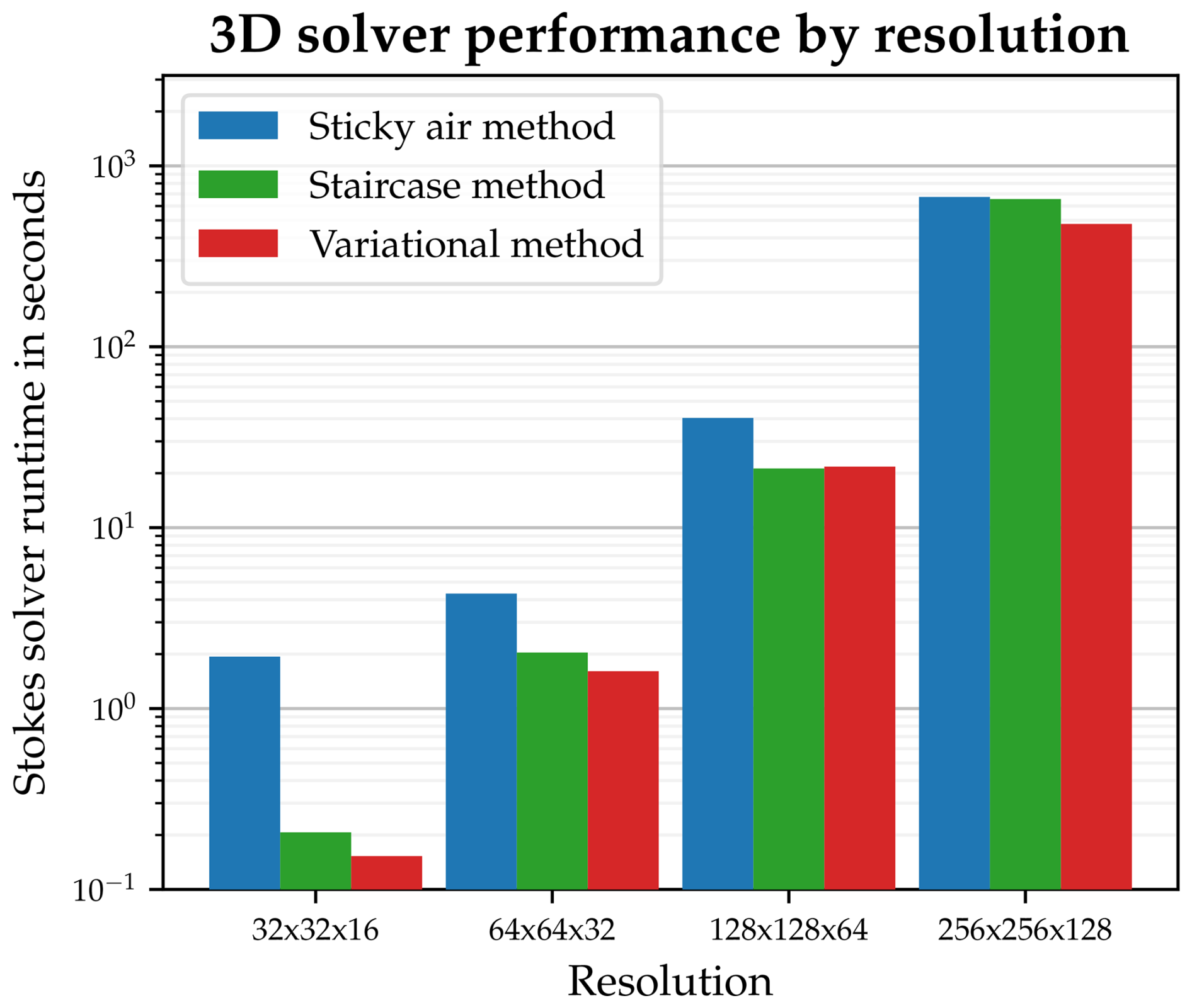
Figure 16 Mean Stokes solver runtime per timestep for 3D scaling tests, conducted using an iterative multigrid solver on a constant-viscosity Cartesian box domain at various resolutions. The variational method consistently outperforms the sticky air method. The staircase method shows variable performance results.

The results of this performance benchmark, which consider the mean time required to solve the Stokes equations per timestep, averaged over 5000 timesteps (8 cores, Ryzen 9 3900XT), reveal that the variational method can provide consistently improved Stokes solver performance in comparison to the sticky air method, with the greatest improvement seen at lower resolutions. At lower resolutions, the staircase method also provided superior performance to the sticky air method, with the exception of the highest resolution used, 256 × 256 × 128. The variational method performed better than the staircase method for all except the 128 × 128 × 64 model, where the performance was similar.

These results demonstrate that the variational method offers a more efficient solution to the Stokes equations with a free surface boundary condition than the sticky air method across all tested cases. This efficiency, coupled with consistent surface tracking performance across resolutions, highlights the potential of the variational Stokes method for 3D geodynamic simulations.

5.6 Prescribed traction boundary conditions

One of the key features enabled by the variational Stokes method is the ability to apply tractions directly at the free surface. This includes the ability to impose pressure boundary conditions at the surface. This capability holds significant potential for applications in global-scale geodynamic models.

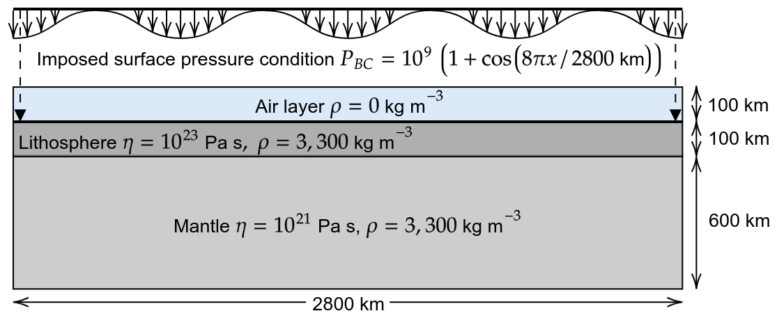
Figure 17 Imposed pressure boundary condition setup in 2D. The model is run at a resolution of 512 × 64 for 4 My to investigate the effect of the imposed surface pressure on topography.

To evaluate the application of imposed traction boundary conditions in 2D, a simple setup illustrated in Fig. 17 is used. The model consists of a 2800 km × 800 km domain run at a resolution of 512 × 64, consisting of an initially flat 600 km thick mantle, a 100 km thick lithosphere, and a 100 km thick air layer. A sinusoidal pressure boundary condition is applied to the free surface, given by:

The imposed pressure boundary condition tested is a sinusoidal profile given by:

$$\begin{array}{}\text{(14)}& P_{\text{BC}}={\mathrm{10}}^{\mathrm{9}}(\mathrm{1}+\cos (\mathrm{8}\mathit{\pi }x/\mathrm{2800}\mathrm{km}\left)\right)\mathrm{Pa}.\end{array}$$

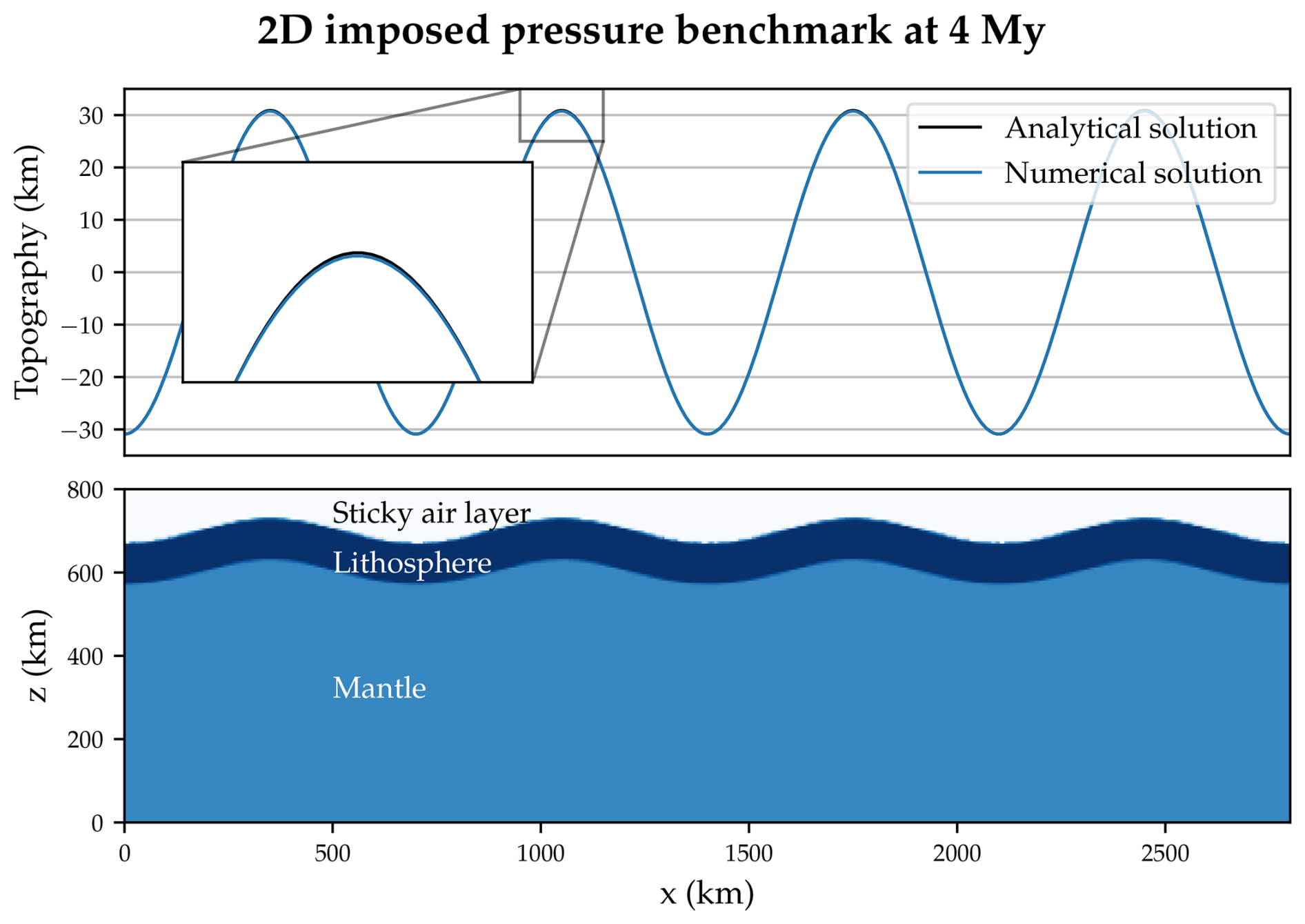
Figure 18 The topography generated by the imposed pressure boundary condition in 2D follows a sinusoidal pattern corresponding to the applied pressure. After 4 My, the numerical solution has almost exactly converged to this analytical solution.

The analytical solution for surface height can be derived using the relationship for lithostatic pressure, P=ρgh, resulting in:

$$\begin{array}{}\text{(15)}& h_{\text{analytical}}={\displaystyle \frac{{\mathrm{10}}^{\mathrm{9}}\cos (\mathrm{8}\mathit{\pi }x/\mathrm{2800}\mathrm{km})\mathrm{Pa}}{\mathrm{3300}\mathrm{km}\cdot \mathrm{9.81}\mathrm{m}{\mathrm{s}}^{-\mathrm{2}}}}.\end{array}$$

The model is run for 4 My to allow surface deformation to reach equilibrium. The resulting topography is compared to the analytical solution in Fig. 18.

The results show that the surface topography relaxes to the predicted analytical solution, exhibiting sinusoidal deformation due to the imposed pressure boundary condition.

6 Summary and discussion

This study has demonstrated the successful implementation of the variational Stokes method of Larionov et al. (2017) within the StagYY geodynamic code and evaluated its performance against the established sticky air and staircase free surface methods. The method is implemented by multiplying the local stencil with appropriate volume fractions, requiring only modest modifications to the Stokes solver. Since these modifications are local, the approach is straightforwardly applicable to other staggered-grid finite difference codes such as I2ELVIS/I3ELVIS (Gerya and Yuen, 2007; Gerya et al., 2015b) or LaMEM (Kaus et al., 2016).

In most scenarios tested, the variational method produces results virtually identical to those of the sticky air and staircase methods, while substantially reducing the computational cost of solving the Stokes equations when using iterative or multigrid solvers. This improvement arises because the variational formulation eliminates the need for an air layer entirely, reducing the size of the system that must be solved. The method is applicable to all 2D and 3D geometries implemented in StagYY, including spherical and yin-yang geometries, making it suitable for global-scale mantle convection models. Accurate volume fractions are best obtained through Lagrangian surface tracking.

A particularly valuable feature of the variational discretisation is its natural support for prescribed traction boundary conditions at the free surface. This capability opens the door to modelling coupled planetary systems in which an external load, such as an ice sheet or ocean, acts on the lithosphere. Phenomena such as post-glacial rebound or the effect of evolving sea levels on lithospheric stress could, for the first time, be incorporated into global-scale geodynamic models with a free surface.

One limitation requires further attention. The treatment of viscosities in cells near the free surface introduces errors when lateral viscosity variations are present, as seen in Sect. 5.3. Since both the present results and the original benchmarks of Schmeling et al. (2008) show that subduction dynamics are highly sensitive to subtle changes in the near-surface viscosity field, existing benchmarks may be insufficient to validate future improvements. Developing more stable benchmarks targeted at near-surface viscosity treatment is therefore an important direction for future work, alongside exploration of alternative viscosity interpolation schemes.