Evaluation of the LandscapeDNDC model for drained peatland forest managements, LDNDC v1.35.2 (revision 11434)

Rotational forestry (RF) is the prevailing management practice on drained peatlands in Finland, while continuous cover forestry (CCF) is increasingly studied for its potential climate benefits. We applied the process-based LandscapeDNDC model, for the first time, to simulate experimental peatland forest stands under three different managements: RF, CCF and non-managed Control. Mixed-species stands of pine, spruce, and birch were initialized, with management, partial harvest of pine in CCF and clear-cut harvest of all species in RF, leading to species shifts toward spruce–birch dominance in CCF and birch seedlings in RF. The primary objective of this study was to evaluate the performance of LandscapeDNDC model in forested drained peatlands. To this aim, we quantified the differences in gas exchange and water balance originating from differences in species composition and management methods. We also implemented modification to dynamic water table (WT) calculations and improved humus pool partitioning based on soil carbon-to-nitrogen ratios. Model evaluation against field data showed strong agreement for daily net ecosystem exchange (correlation 0.84–0.88; Nash–Sutcliffe efficiency 0.66–0.75). Modeled leaf area index (LAI) closely matched site estimates before management and Sentinel-2 satellite estimated LAI afterwards. Soil moisture and WT dynamics were realistically reproduced. Methane flux patterns were accurately captured in the control and CCF stands. Moreover, the methane flux was found to be sensitive to the WT after clear-cut in the RF stand. Modeled annual carbon balances were consistent with measurements and indicated that CCF became a carbon sink more rapidly than RF. These results demonstrate that LandscapeDNDC can reliably simulate the biogeochemical and hydrological consequences of alternative peatland forest management scenarios. The model therefore provides a valuable tool for developing climate-smart management strategies on drained peat soils.

1 Introduction

Peatlands cover 3 % of the land area on Earth (Clarke and Rieley, 2019). The amount of carbon stored in northern peatlands is estimated to be around 1016–1105 Gt (Nichols and Peteet, 2019). Peatlands are often drained for use in forestry, agriculture, and peat extraction (Clarke and Rieley, 2019). In Finland, peatland drainage began in the 1920s and increased significantly in the 1960s. The drainage of peatlands expands the land area available for forestry, facilitating tree growth in regions that were previously unsuitable for productive forest development. However, draining peatlands leads to increased aeration and degradation of the peat, which increases carbon dioxide (CO₂) emissions from the soil due to increased peat decomposition (Findlay, 2021). Forests on drained peatlands make up 25 % (5.7 Mha) of the total forested land area in Finland (Turunen and Valpola, 2020).

Forest ecosystems on nutrient rich soils have been significant CO₂ source (Ojanen et al., 2013; Lohila et al., 2007) to a small sink (Korkiakoski et al., 2023). Forest ecosystems on nutrient poor soils on the other hand have been moderate sink (Tong et al., 2024) to high sink (Laine et al., 1996; Lohila et al., 2011; Minkkinen et al., 2018). However, it may take decades for forest ecosystems to reach a net CO₂ sink after drainage, if it is reached at all (Quesada et al., 2026). Carbon-to-nitrogen ratio (C:N) is an often-used indicator for the nutrient status of peat soil and it is typically lower in drained nutrient rich peat. Decomposition of peat releases nutrients available to plants, and this nutrient input decreases from rich to poorer sites (Baylay et al., 2005). Peat soils on drained nutrient-rich sites tend to be sources of CO₂ (He et al., 2016; Kasimir et al., 2018), while in nutrient-poor sites may act as a carbon sink (Ojanen et al., 2013).

Carbon storage of the forest ecosystem is also subject to management practices. When the forest is harvested, most of the carbon stored in wood is rapidly lost to the atmosphere if the harvested wood is used for short-lifetime products such as pulp or energy production (Makrickas et al., 2023). Therefore, a peatland forest, whose soil is a net CO₂ source, has a climate warming impact over the entire forest rotation period, even though it may be a net CO₂ sink at a moment in time.

The most common forest management method implemented in Nordic countries has been Rotational Forestry (RF). In RF, forests are clear-cut when a specific stand volume has been reached and new stands are usually established by planting seedlings on the harvested land (Nieminen et al., 2018). Before planting new seedlings, the harvested land is sometimes fertilized and mounded, and often the mounding material comes from ditch maintenance (Hytönen et al., 2020). Harvest residues (litter, small branches, tree roots and stumps from the previous forest) are often left on the site or removed. Recently, more importance has been given to the investigation and implementation of alternative forestry management methods that would decrease carbon losses from the soil while maintaining profitable timber production. Continuous Cover Forestry (CCF) has been suggested as a management practice that could be applied to reach this goal (Nieminen et al., 2018). In CCF, the forest is never clear-cut as in RF, but rather selectively harvested depending on the forest and soil characteristics, resulting in an unevenly aged forest structure.

In drained peatlands, vegetation growth influences the water table (WT) significantly through evapotranspiration. Increased biomass, particularly from deep-rooted trees, promotes water loss and leads to a decrease in WT (Laiho, 2006). In CCF the WT remains higher than in the full-grown forest, because non-harvested mature forest has higher evapotranspiration compared to the forest where a selective harvest has been conducted (Sarkkola et al., 2010). Higher WT in CCF results in reduced peat degradation and minimizes carbon loss from the soil. In CCF, however, the remaining trees continue to transpire water and keep the WT low enough that WT does not hinder forest growth (Nieminen et al., 2018). While in RF, after clear-cut, WT rises significantly because of lack of transpiring vegetation (Leppä et al., 2020) and often requires ditch management to lower the WT before planting new seedlings.

The Lettosuo site, a drained nutrient rich peatland forest in Southern Finland, had both selective harvest and clear-cut management applied to the site to convert part of the site into a CCF stand and another part into a RF stand (Leppä et al., 2020). Measurements of the net ecosystem carbon exchange in Lettosuo showed the mature forest to be a small sink of CO₂ before harvest (Korkiakoski et al., 2023). After harvest, RF stand was a bigger CO₂ source compared to the CCF stand (Korkiakoski et al., 2023). The same site was a sink for methane (CH₄) before harvest (Korkiakoski et al., 2017), and after selection harvest (Korkiakoski et al., 2020) due to low WT. However, RF stand was a source of CH₄ after clear-cutting due to raised WT (Korkiakoski et al., 2019). An increase in WT could lead to higher anaerobic conditions in the soil layer that promotes methanogenesis and eventually even turn drained peatlands into a net CH₄ source (Lohila et al., 2011). Further, temporal and spatial variations of CH₄ can be attributed to the dynamics of soil temperature, soil moisture, and vegetation communities (Minkkinen and Laine, 2006).

Apart from being a major habitat, peatland systems have challenged terrestrial ecosystem models (Mozafari et al., 2023; Silva et al., 2024), for example because of their dynamic water table regulating carbon processes (e.g. Mezbahuddin et al., 2017), or specific ground vegetation (e.g. Shi et al., 2021). Only in recent years, specific processes for peatlands have been given more consideration (e.g. Liu et al., 2022; Li et al., 2024). The process-based ecosystem model LandscapeDNDC has been used to simulate carbon and water balances in various forest systems, including monoculture (Werner et al., 2012; Dirnböck et al., 2016), structured forests with ground vegetation (Dirnböck et al., 2020; Cade et al., 2021) and managed forests (Grote et al., 2011). The simulations mentioned above considered sites with mineral soils, whereas applications on peat soils are still lacking.

The primary objective of this study is to evaluate the performance of LandscapeDNDC model in forested drained peatlands. To address this objective, we refined and employed a process-based model, applied here for the first time to a nutrient-rich drained peatland in Finland. Refinements to the dynamic WT and high carbon content are investigated using carbon and water flux measurements. We perform a sensitivity analysis to determine the most sensitive parameters for decomposition in carbon rich soil. We assess how variations in tree species composition and management methods influence gas exchange and water balance. The model improvements should allow for a realistic representation of the forest CO₂ and CH₄ budgets, soil hydrology, and soil carbon balances within the drained peatland forest systems. Ultimately, the study aims not only to test the model's applicability and accuracy for Lettosuo study site but also to provide a foundation for assessing future peatland management scenarios. This approach supports the broader goal of identifying climate-smart forest management strategies that contribute to carbon neutrality on drained peat soils.

2 Material and methods

2.1 Model description

The simulation framework LandscapeDNDC has been developed to allow a flexible problem-specific model composition for the simulation of the water, carbon and nitrogen cycles in cropland, grassland and forest ecosystems (Haas et al., 2013). In this study, the microclimate within the forests is simulated using the sub-model CanopyECM according to Grote et al. (2009). Vegetation related processes are modeled with the Physiological SImulation Model (PSIM) sub-model (Grote et al., 2006, 2011). Soil biogeochemical processes were represented with the MeTr^x sub-model (Kraus et al., 2015), while soil hydrological conditions are represented with the Ecosystem Hydrology (EcHy) sub-model (Dirnböck et al., 2020).

PSIM enables the representation of a multiple species stand, where individual tree species can have their own characteristics and dimensions, while also having interactions with each other (Cade et al., 2021). Including multiple species in the simulation allows to consider the contributions of dominant trees, understorey and ground vegetation to carbon and water fluxes. In particular, the importance of understory in boreal forests has been highlighted before and is thus necessary to be included in the model (Korkiakoski et al., 2023; Leppä et al., 2020).

The soil sub-model MeTr^x accounts for carbon and nitrogen pools and fluxes and their responses to land use and forest management. Most relevant processes considered by MeTr^x for this study are humification, mineralization, nitrification and denitrification as well as CH₄ production and consumption (Kraus et al., 2015). In MeTr^x, various litter (Solutes, Cellulose and Lignin) and humus (Labile, Recalcitrant young and old) pools are differentiated according to their chemical structure (Kraus et al., 2015) and carbon to nitrogen ratio, respectively. These organic materials are decomposed by microbial pools in the nitrification and denitrification processes. Besides pool size and organic matter properties, processes depend on the availability of oxygen, pH, clay content, soil temperature and soil moisture. MeTr^x also covers CH₄ production as a final step at the end of decomposition under anaerobic conditions as well as CH₄ transport from air to soil and CH₄ oxidation. Oxygen content is dynamically calculated for each soil layer. Detailed descriptions of these processes can be found in Kraus et al. (2015), Molina-Herrera et al. (2015), and Haas et al. (2022). Soil water dynamics are calculated by the EcHy module, which predicts a dynamic groundwater table (z_gw) depending on the simulated water balance. In its conceptual design, EcHy is a one-dimensional (1-D) vertical soil column model. When applying its original version in this study, the simulation domain became waterlogged because precipitation exceeded evapotranspiration and percolation through the lower soil boundary. In reality, however, the site is drained by ditches that induce a lateral water flow component and counteract complete soil saturation. To account for this, a reference water table (Z_gw) was introduced, which represents the depth below which no significant lateral flow occurs (e.g. the ditch depth), and the soil is assumed to be fully saturated. In addition, a parameter Ψ representing lateral groundwater flow velocity and ditch distance was implemented. This parameter determines the rate of lateral water loss whenever the simulated dynamic water table depth z_gw is above Z_gw. Together, these modifications introduce a lateral (2-D) flow component into an otherwise 1-D framework, enabling EcHy to better reflect local site conditions. Lateral groundwater movement q is given by,

$$\begin{array}{}\text{(1)}& {\displaystyle }{\displaystyle }q=max(\mathrm{0.0},|Z_{\text{gw}}-z_{\text{gw}}\left|\right)\times \mathrm{\Psi }\times K_{\mathrm{s}}\end{array}$$

z_gw: depth of groundwater in m, Z_gw: depth of reference groundwater in m, Ψ: Model parameter representing lateral groundwater gradient m⁻¹, K_s: the saturated hydraulic conductivity of the last soil layer m min⁻¹.

In the model, soil organic matter is represented by three conceptual humus pools (labile, recalcitrant young, recalcitrant old) differing in turnover time and C:N ratio. The C:N ratio of the young recalcitrant pool is 1.5 times the bulk soil C:N ratio, which is the model's default parametrization for agricultural (mineral) soils. Peat soils in this study are characterized by systematically higher bulk C:N ratios than mineral soils. For peat, we interpreted the young recalcitrant pool as the main peat pool and therefore aimed to reduce the initial relative share of the old recalcitrant pool compared to mineral soils. To achieve this while conserving bulk soil C and N, we assigned a lower C:N ratio to the old recalcitrant pool than to bulk soil, which reduces the amount of C that is allocated to old recalcitrant pool. The C:N ratio of the recalcitrant old pool (CN_rec) is scaled as a function of the bulk soil C:N ratio (CN_bulk):

$$\begin{array}{}\text{(2)}& {\displaystyle }{\displaystyle }{\text{CN}}_{\text{rec}}=(\mathrm{0.9}-max(\mathrm{0},\mathrm{0.8}-\mathrm{8}\times {\text{CN}}_{\text{bulk}}\left)\right)\times {\text{CN}}_{\text{bulk}}\end{array}$$

When CN_bulk very large:

$$\begin{array}{}\text{(3)}& {\displaystyle }{\displaystyle }{\text{CN}}_{\text{rec}}=\mathrm{0.1}\times {\text{CN}}_{\text{bulk}}\end{array}$$

When CN_bulk≤10:

$$\begin{array}{}\text{(4)}& {\displaystyle }{\displaystyle }{\text{CN}}_{\text{rec}}=\mathrm{0.9}\times {\text{CN}}_{\text{bulk}}\end{array}$$

This formulation therefore reduces the size of the old recalcitrant humus pool with increasing soil C:N ratio. Changes to the model code can be found from Butterbach-Bahl et al. (2026).

2.2 Site description

Lettosuo site, located in southern Finland ($\mathrm{60}\mathit{°}{\mathrm{38}}^{\prime }{\mathrm{31}}^{\prime \prime }$ N, $\mathrm{23}\mathit{°}{\mathrm{57}}^{\prime }{\mathrm{35}}^{\prime \prime }$ E), covers a total area of 65 ha (Fig. A1). The site, extensively drained in 1969 using ditches that were 45 m apart, is classified as a nutrient-rich Vaccinium myrtillus type II forest (MtkgII, Laine, 1989). Lettosuo was originally a sparsely treed, mesotrophic pine-birch sedge fen rich in herbs (Korkiakoski et al., 2023). Fertilizers were used after drainage to help with the growth of existing pine (Pinus Sylvestris) trees. In the 1970s and later, some thinning was done to ensure better growth of pine, but those thinning information are unavailable. Over time Lettosuo became a mixed forest site, where pine and birch (Betula Pendula) formed the overstory and spruce (Picea Abies) formed the understory canopy. The forest floor consisted of various herbs, shrubs and graminoids (Korkiakoski et al., 2023).

The site was divided into three sections according to the applied management methods: a control stand where no management action had taken place; a Continuous Cover Forestry (CCF) stand where all the pine trees (75 % of the original total biomass) were harvested in March 2016 (Korkiakoski et al., 2020); and a Rotational Forestry (RF) stand where all the trees were removed by clear-cutting, also in March 2016 (Korkiakoski et al., 2019).

In RF, the application of heavy harvesting machinery destroyed the forest floor vegetation, while in CCF, forest floor vegetation was only affected on logging trails. In RF, the harvest residues were left at the felling area, while in CCF, the harvest residues were placed on the logging trails. At RF, ditches were maintained after clear-cut and peat extracted from the ditches was used to form mounds of peat soil where new spruce seedlings were planted in 2017. Most of the spruce seedlings died during the drought in 2018 (Korkiakoski et al., 2023). Later naturally occurring birch seedlings became the dominant species at RF stand.

2.3 Site observations and auxiliary data

2.3.1 Model driving data

Finnish Meteorological Institute's long-term (1963–2021) observation-based meteorological data were used to drive the model (Aalto et al., 2016). Meteorological data consisted of temperature, precipitation, global radiation, wind speed and relative humidity. Nitrogen deposition, in the form of ammonium and nitrate wet deposition, was selected to match values (6 $\mathrm{kg}{\mathrm{ha}}^{-\mathrm{1}}{\mathrm{yr}}^{-\mathrm{1}}$) for the northern latitudes (Harmens et al., 2011). Background CH₄ concentrations were set at a constant value of 1.74 ppb. The CO₂ concentration used to drive the model was based on observations up to 2005 and follows RCP4.5 since then (i.e. historical + scenarios), and deviates from the observed value by 1.3 ppm by 2021 (Meinshausen et al., 2011).

2.3.2 Model evaluation data

One-sided Leaf Area Index (LAI) was estimated from Sentinel-2 satellite data for all stands and mostly consisted the post harvest years (Nevalainen, 2022; Korkiakoski et al., 2023). Additionally, the modeled pre-harvest LAI was compared against site estimated LAI reported by Leppä et al. (2020).

Data from the control stand included CH₄ fluxes, which were measured with six automatic chambers from June 2015 to January 2019. WT measurements at control stand covered the years 2016–2021 (Korkiakoski et al., 2020). The soil moisture content measurements at depths of 10 and 20 cm covered the duration from July 2015 to January 2019.

Eddy-covariance (EC) measurements of CO₂ exchange between the ecosystem and the atmosphere, i.e. net ecosystem exchange (NEE), were conducted on top of a telescopic mast (height 25.5 m until June 2019 and later at 27.2 m) at CCF stand. NEE before selective harvest will be referred to as pre-harvest and after selective harvest will be referred to as CCF_postharvest. The pre-harvest data covered the time period from January 2010 to March 2016 and CCF_postharvest from April 2016 to December 2021. Gross primary production (GPP) and total ecosystem respiration (TER) were estimated from the NEE data (Korkiakoski et al., 2023) and used in this study to evaluate the LandscapeDNDC model performance. CH₄ measurements from the CCF stand were conducted with six automatic chambers from May 2015 to May 2018 (Korkiakoski et al., 2020), i.e. one year before the harvest and three years after the harvest. These were used to validate the CH₄ fluxes from CCF simulation. CCF also had continuous WT measurement from January 2010 to December 2021 (Korkiakoski et al., 2023).

A separate EC tower (height 3.2 m) in the rotational forestry stand was set up after the clear-cut harvest in March 2016 (Korkiakoski et al., 2019). NEE measurements from the RF after clear-cut, will be referred to as the RF_postharvest. NEE, GPP, TER and WT data from April 2016 to December 2021 were used in this study to evaluate the model. CH₄ fluxes were measured with the manual chambers and covered the period of May 2016–September 2017 (Korkiakoski et al., 2019).

2.4 Simulation setup

In the simulations, the vertical soil profile was divided into several layers of increasing thickness with increasing layer depth (Table 1). The carbon and nitrogen content, bulk density and pH of the soil layers were taken from the measured Lettosuo data previously reported by Leppä et al. (2020) and Korkiakoski et al. (2017). These soil variables and their prescribed initial levels are given in Table 1.

Table 1 Soil layer profile from the measured Lettosuo data previously reported by Leppä et al. (2020) and Korkiakoski et al. (2017) used for simulations, where soil depth in cm, Carbon (C) content, Nitrogen (N) content, Bulk density (BD), Carbon to Nitrogen ratio (CN), pH, van Genuchten parameters n and α, and minimum water filled pore space (WFPS_min), are given as,

The simulations initialized with pristine peatland condition from 1969. During the first three simulation years fluctuations in litter and humus pools were stabilized. During this period, the Z_gw was set to 0.01 m depth to stabilize the soil carbon pools for pristine peatland condition. In the case of pristine peatland simulation, to study the soil carbon changes, the Z_gw was kept at 0.01 m until 2021. Otherwise, for forest stand simulations, Z_gw was set to 0.62 m after initial three years to represent drained peatland conditions. The model then simulated WT dynamically with the modification described in Sect. 2.1.

The initialization of tree species and forest floor vegetation is presented in Table 2. The simulations began in 1969 with pine trees and the forest floor vegetation. Birch and spruce were added in 1971 and 1972, respectively. Management events (selective harvest and clear-cut) took place in 2016. Harvest residues were left in the simulation domain and stemwood biomass was removed after management events. All simulations were run until end of 2021. All the modules were run with a sub-daily time step (30 min) and sub-daily and daily simulation outputs were used for various investigations.

Table 2 Individual species were introduced to the simulations starting from 1969. In non-managed control no species were removed and continuation of species until the end of simulation is indicated by –. In Continuous Cover Forestry (CCF) pine was removed during selective harvest, while in the Rotational Forestry (RF) all species were removed during clear-cut (RF_CC). Individual species were reintroduced for a new forest in RF (RF_{New forest}) with the number of seedlings RF_{Newforest, n} reported by Korkiakoski et al. (2019).

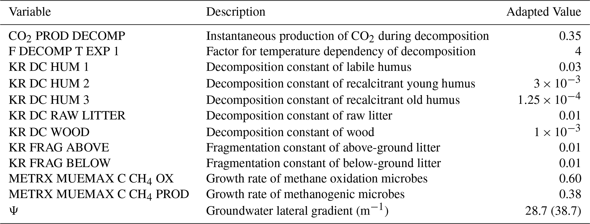
The sensitivity of NEE to soil decomposition was tested with separate one-year mature forest simulations for a range of soil parameters (Table A1) described in Sect. 2.6 and Appendix A2. For this study species parameters reported in Grote et al. (2011), a study which simulated a mixed forest stand consisting of pine, spruce and birch trees on mineral soil in southern Finland, were used and adjusted to run the sensitivity test simulations and full forest simulations (Table A2). These parameters included e.g. photosynthesis related VCMAX (Maximum RubP saturated rate of carboxylation at 25 °C for sun leaves), KM20 (Maintenance coefficient at reference temperature), SLAMAX (Specific leaf area in the shade) and SLAMIN (Specific leaf area in the full light). Several sensitive soil parameters related to the decomposition of different humus and litter pools were later adjusted during full forest simulations (Table A3).

2.5 Model data analysis and evaluation

The correlation coefficient (r) and Nash–Sutcliffe efficiency (NSE) were calculated from the daily aggregate of the available measurements and corresponding modeled data. NSE values can vary from −∞ to 1. Model output that produces an NSE value of 1 is described as the perfect simulation, thus NSE values closer to 1 are desirable.

NSE is defined as,

$$\begin{array}{}\text{(5)}& {\displaystyle }{\displaystyle }\text{NSE}=\mathrm{1}-{\displaystyle \frac{{\sum }_{i=\mathrm{1}}^n{\left(Q_{{\mathrm{o}}_i}-Q_{{\mathrm{m}}_i}\right)}^{\mathrm{2}}}{{\sum }_{i=\mathrm{1}}^n{\left(Q_{{\mathrm{o}}_i}-\stackrel{\mathrm{‾}}{Q_{\mathrm{o}}}\right)}^{\mathrm{2}}}}\end{array}$$

Where, Q_o represents the observed data at time i, Q_m represents the modeled data at time i, $\stackrel{\mathrm{‾}}{Q_{\mathrm{o}}}$ is the mean of the observed data. n is the total number of observations.

We further used Root Mean Square Error (RMSE) to quantify the differences between the model and the observations for NEE and WT. In this analysis, seasons are defined as December–January (winter), March–May (spring), June–August (summer) and September–November (autumn).

Since a single simulation setup was used for all three forest stand simulations before the harvesting events, both measured and simulated data will be referred to as pre-harvest data (2010–2015). Korkiakoski et al. (2023) calculated the annual CO₂ balances (NEE, GPP and TER) for 2016 from April 2016 to March 2017 and the modeled estimates for 2016 were also calculated similarly in the CCF_postharvest and RF_postharvest. To show the sensitivity of the simulated CH₄ flux with WT after clear-cut harvest, the groundwater lateral gradient parameter was changed (28.7–38.7 m⁻¹, Table A3) in the simulation to reproduce the lowest and highest observed WT at RF (Sect. 3.3).

The effect of drainage on the simulated soil carbon (SC) storage was compared to the SC loss reported by Simola et al. (2012). The influence of harvesting, under different management methods, on SC dynamics was assessed by quantifying changes in SC following harvest. This included investigating the partition of different litter (solutes, cellulose and lignin) and humus (labile, recalcitrant young and old) pools. The evolution of the total carbon (soil carbon + carbon in vegetation) over the whole simulation period was also studied (Sect. 3.5). A pristine peatland simulation, without any drainage or harvesting, served as a reference. Data and Python codes used in this study can be found from Shahriyer (2025a, 2026a, b).

2.6 Sensitivity test

Sensitivity analyses of soil parameters were conducted separately using mature forest stands in one-year simulations. The analyses were performed with the Python library SPOTPY and its Fourier Amplitude Sensitivity Test (FAST) algorithm (Houska et al., 2015, 2017). The sensitivity analyses were carried out sequentially, with the best-performing parameter values from each stage retained for subsequent analyses. The soil parameters were divided into three sets, each containing nine parameters, and the parameter ranges tested are presented in Table A1. The three parameter sets represented (1) decomposition rate constants for different soil pools, (2) factors describing the dependence of decomposition on environmental conditions and (3) humification factors for different soil pools. Rather than varying all parameters simultaneously, only one set was varied at a time, while the remaining parameters were fixed at either their default values or values determined from the preceding sensitivity analysis. The number of simulations performed for each parameter set was considered sufficient to provide robust sensitivity estimates. During all sensitivity analyses, species parameters were held constant using the values presented in Table A2.

For the first analysis, the nine decomposition rate related soil parameters in Set 1 were evaluated using 8649 model runs generated by FAST algorithm (Houska et al., 2017). Parameter values in Set 1 were sampled automatically within their predefined ranges, while all parameters in Sets 2 and 3 were fixed at their default values (Table A1). Following the first sensitivity analysis, the modeled NEE from all runs was compared against measured NEE to determine the parameter values for Set 1 to be used in subsequent analyses. The parameter values from the run that yielded the highest NSE were extracted (Table A1). These values were then fixed for the Set 1 parameters during the sensitivity test runs for Set 2. During the second sensitivity analysis, parameter values in Set 2 were again sampled by FAST algorithm and the parameters in Set 3 had default values. As in the first analysis, the parameter values from the run yielding the highest NSE were extracted in second analysis and subsequently fixed for the parameters in Set 2 when the sensitivity test runs for Set 3 was performed. The third sensitivity analysis was conducted by varying the nine parameters in Set 3 while keeping the selected parameter values from Sets 1 and 2 fixed. The parameter values corresponding to the highest NSE obtained in the third analysis are also presented in Table A1. The results of these analyses are presented in the Appendix (Table A1, Figs. A2–A4 and S1–S3 in the Supplement).

The sensitivity analysis of the first parameter set indicated that the decomposition rate constant for the recalcitrant young humus pool was the most influential parameter affecting modeled NEE (Fig. A2). Other highly sensitive parameters in this set were associated with the decomposition of labile humus, recalcitrant old humus, raw litter, and the effect of litter lignin concentration on decomposition. In the second parameter set, the most sensitive parameters were those describing the effects of temperature and pH on decomposition, as well as the reduction in decomposition under anaerobic conditions (Fig. A3). For the third parameter set, the most influential parameters were related to the C:N ratio of the old humus pool relative to the overall soil C:N ratio. Other sensitive parameters were the humification rate of recalcitrant young humus, dissolved organic carbon, active organic matter, and solutes (Fig. A4).

The sensitivity analyses were conducted solely to evaluate parameter sensitivity, and the resulting parameter values were not directly adopted for the full forest simulations. Instead, long-term simulations from seedling establishment to stand maturity were performed separately using a limited number of selected soil parameters, whose values were chosen to reproduce the observed tree species composition at the study sites (Table A3). The species-specific parameter values used in these simulations are provided in Table A2.

Particular attention was given to the calibration of the full forest simulations because relatively small changes in soil parameter values could alter competitive interactions among tree species and thus lead to forest compositions that differed from those observed in the field. As the primary objective of the study was to reproduce the observed forest structure, parameter values were selected to maintain realistic stand development and species composition. In contrast to the sensitivity analyses, where model performance was assessed solely using the NSE of simulated NEE, the evaluation of the full forest simulations considered multiple variables. These included NEE, soil moisture, WT, LAI, CH₄ fluxes, and forest structure, all of which were compared with available measurements.

A comprehensive optimization procedure incorporating all evaluated variables would have been desirable; however, the computational demands of the full forest simulations were substantial. Consequently, parameter selection for the full simulations was based on an overall assessment of model performance across the observed ecosystem characteristics rather than on formal multi-objective optimization.

3 Results

3.1 Development of forest structure before and after management

In the forest stand simulations, the model accurately reproduced the observed range of species-specific tree numbers at stand age 45 (Table 3). The height of the individual species was also close to the observed values. The modeled pine and spruce volumes were close to the observed volume ranges, while birch had 27 % less volume. The model successfully reproduced the reported pre-harvest LAI of the different tree species in 2014 (Fig. 1a). Forest floor vegetation had modeled LAI of 0.94 m² m⁻² in August 2014, which was similar to the observed LAI of 1 m² m⁻² reported by Leppä et al. (2020). The same literature reported LAI for above ground canopy (pine + spruce + birch) to be 4.66 m² m⁻² and the corresponding modeled LAI was 4.68 m² m⁻² (August 2014; Table 3).

Table 3 Comparison between simulated vegetation structure with observations before management at stand age of 45 years (August 2014). Simulated outputs are shown in bold. Tree numbers (n ha⁻¹), tree heights and stand volumes collected by Korkiakoski et al. (2023) from Lettosuo site are given in parenthesis. SD is the standard deviation. Simulated individual tree species diameters are given in bold. LAI estimates for individual species reported by Leppä et al. (2020) are given in parenthesis.

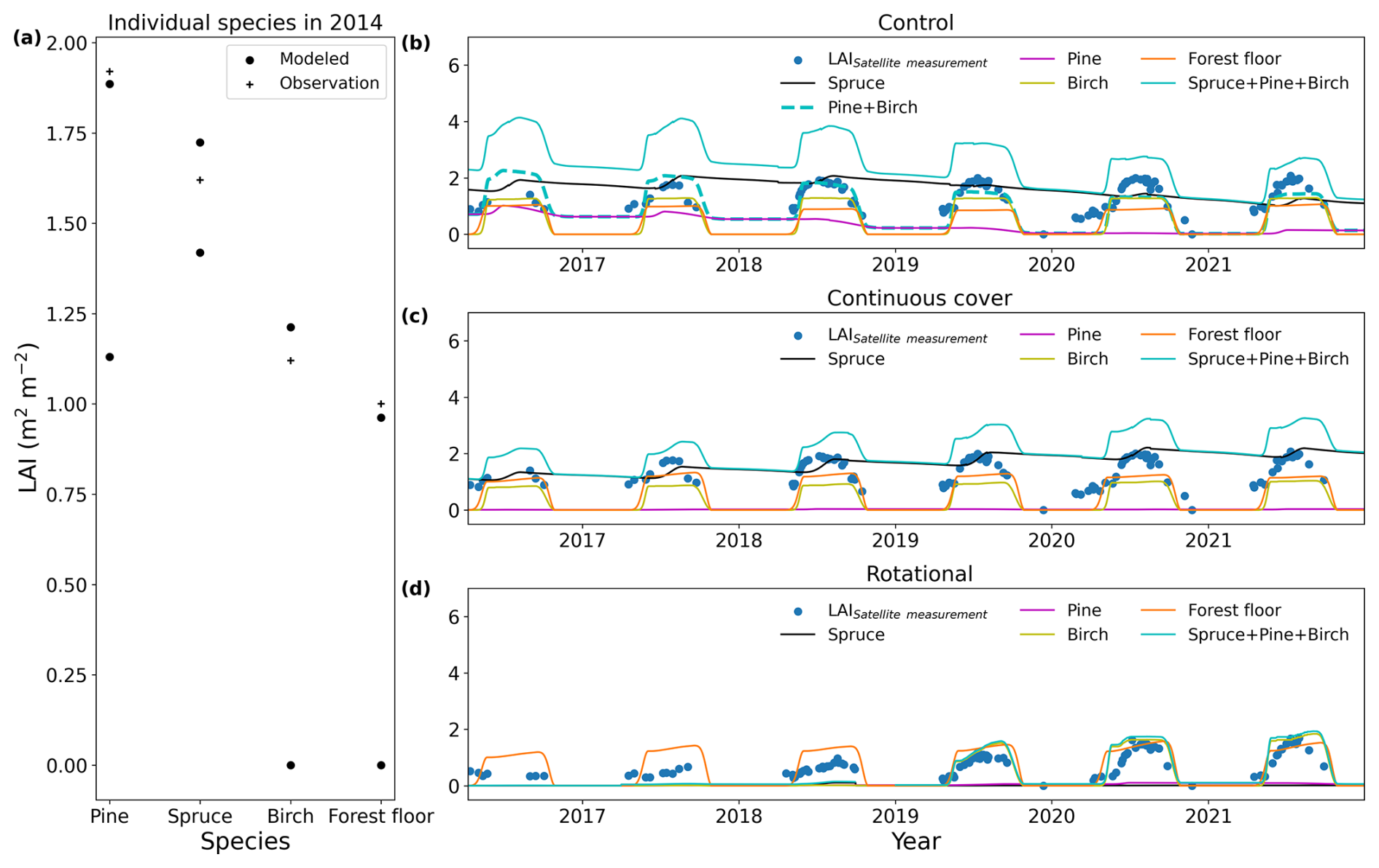
Figure 1 (a) One-sided Leaf Area Index (LAI) estimates for individual species from field observations (plus) (Leppä et al., 2020) compared to minimum and maximum modeled LAI (circles) in 2014 for a 45-years-old forest. (b), (c), and (d) show LAI development in different management scenarios, where modeled LAI are represented by solid and dashed lines and satellite-estimated LAI by blue dots. (b) Pine + Birch LAI are represented with dashed lines only for control simulation.

Modeled pine and spruce LAI were diminishing from 2016 to 2021 for control simulation (Fig. 1b), which was not seen in the prior six years (Fig. S4 in the Supplement). The sum of pine and birch modeled LAI was closest to the satellite-based LAI (Fig. 1b), and this could be realistic since pine and a small percentage of birch were forming the upper-story canopy in the control stand. The gradual decline in modeled LAI from 2016 to 2021, evident in control simulation, was not seen in the CCF simulation. In fact spruce LAI continued to increase until 2021, likely a result of reduced competition between species owing to the removal of pine during harvest (Fig. 1c). Spruce LAI during summer months was closer to satellite-based LAI, while the sum of spruce and birch modeled LAI was always larger than the satellite-based LAI (Fig. 1c). The modeled LAI for birch and forest floor remained consistent from 2016 to 2021 for both control and CCF. After clear-cutting in RF, the modeled LAI was almost double the satellite-based LAI in 2016, whereas the discrepancy between the two decreased progressively after 2018 (Fig. 1d). Simulated birch and forest floor LAI were closest to satellite-based LAI in 2019–2021 (Fig. 1d).

3.2 Dynamics of soil moisture, water table

The model reproduced soil moisture dynamics well during the growing seasons of 2015–2017 (May–September), but deviations from the measurements were evident in 2018 (Fig. 2). The model captured the dynamics of 10 cm soil moisture for 2016 and 2017 best. However, the model slightly underestimated soil moisture at a depth of 10 cm in 2015 and overestimated it in 2018 relative to the measurements. At a depth of 20 cm, agreement between simulated and measured soil moisture was strongest during 2015–2017, whereas the model overestimated soil moisture from July 2018 onward.

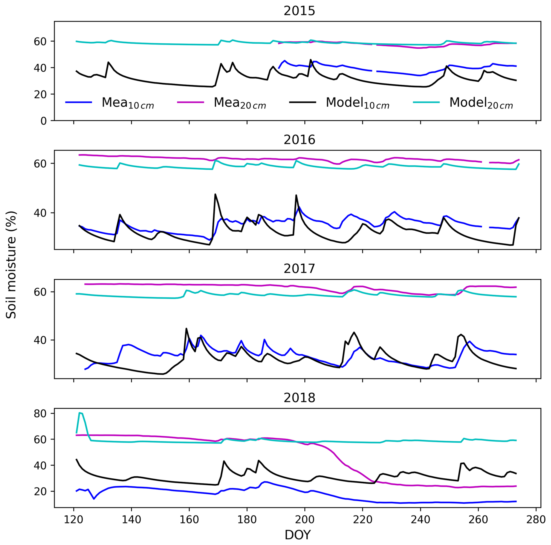
Figure 2 Simulated and measured soil moisture (volumetric moisture content) for the control stand from the beginning of May to the end of September shown in day of year (DOY). Blue and magenta lines show measured soil moisture at 10 and 20 cm depths, respectively. Black and cyan lines show the simulated soil moisture at 10 and 20 cm depths, respectively.

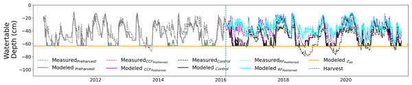
Simulated WT during the pre-harvest period (2010–2015) was in good agreement with the observations at the CCF stand (Fig. 3a). Deviations between the simulated and measured mean WT were most pronounced during the summer of 2016 and 2017 (see also Fig. S5 in the Supplement). From 2018 onward the simulated WT in CCF stand was again similar to the observed WT. The model also predicted the control stand WT within the observed range and reflected the observed dynamics (Fig. 3b). Deviations between simulated and observed WT were most pronounced in the control stand during the autumn of 2018 and 2019 (see also Fig. S6 in the Supplement). At the RF stand, the simulated WT closely followed the observed temporal dynamics and showed relatively small deviations from the measurements (Fig. 3c; see also Fig. S7 in the Supplement). Consistent with the observations, the model predicted a rise in WT after clear-cutting at the RF stand as a result of reduced transpiration following biomass removal. In contrast, the effect of selective harvesting on WT at the CCF stand was minor (Fig. 4), and the differences between simulated and observed WT following harvest, which were evident in 2016 and 2017, largely disappeared in later years.

Figure 3 Water table (WT) dynamics in the (a) continuous cover forestry stand (CCF, includes pre-harvest and post-harvest WT), (b) control stand, and (c) rotational forestry (RF) stand. Blue and black lines represent the mean measured and simulated WT depth, respectively. Gray dashed lines show the range of measured WT from different WT loggers at the CCF and control stand. The blue vertical dashed line shows when the selective harvest took place at the CCF stand. Negative values represent WT below the soil surface.

Figure 4 Simulated (solid) and measured (dashed) water table at pre-harvest (gray), Control (black), CCF_postharvest (magenta), RF_postharvest (cyan) conditions. Additionally the reference water table (Z_gw) shown in orange and vertical dashed line shows the time of harvest.

3.3 Methane flux comparison and sensitivity with water table

Manual chamber measurements indicated that the RF stand became a CH₄ source during the summer months following clear-cutting, whereas the initial RF simulation suggested that the site remained a CH₄ sink during the same period. Although temporal and spatial variability in CH₄ fluxes can be attributed to the dynamics of WT, soil temperature and vegetation communities (Minkkinen and Laine, 2006) and in dry conditions to the wind speed (Korkiakoski et al., 2017) and soil temperature (Sundqvist et al., 2014), only the role of WT was investigated further in this study. The model results showed that CH₄ fluxes were highly sensitive to WT variations after clear-cutting. To examine this sensitivity, two alternative WT scenarios were simulated by modifying the groundwater lateral gradient parameter (Ψ) while keeping the reference WT (Z_gw) unchanged. Altering Ψ had little effect on simulated WT before clear-cutting but resulted in distinct WT dynamics after harvest. No additional modification to the model setup were required to produce this shift in WT. The two WT scenarios generated in the CH₄ sensitivity analysis were also consistent with the lowest and highest WT values observed at the RF stand (Fig. 5). Simulation with the original value (Ψ=28.7 m⁻¹, Table A3), produced the lowest WT, led to a higher sink of CH₄. While the modified parameter value (Ψ=38.7 m⁻¹) produced a higher WT and resulted in smaller sink of CH₄. In the high-WT simulation, the site even acted as a CH₄ source on some occasions. In both RF simulations, modeled CH₄ fluxes showed only minor difference before harvest and represented a weaker CH₄ sink than that observed in the measurements (Fig. 5).

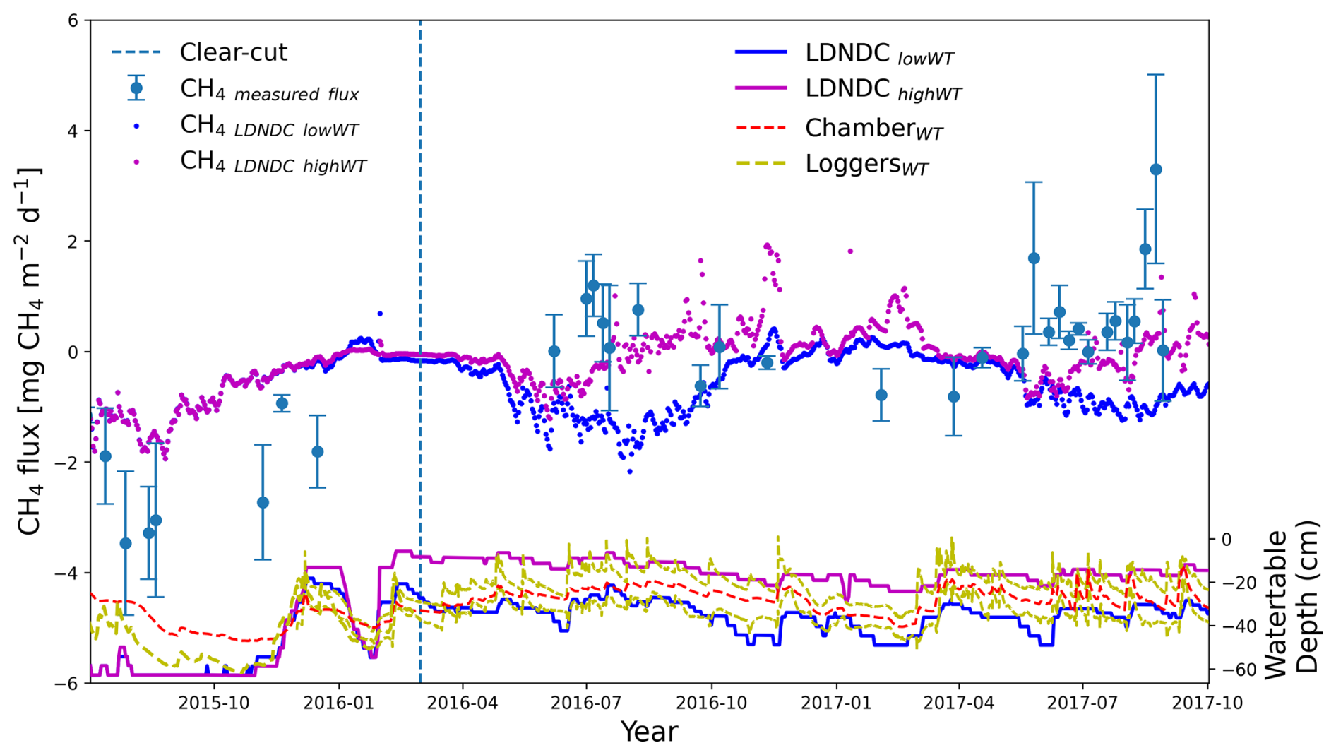
Figure 5 Manual chamber CH₄ flux measurements are represented by light blue dots and associated standard deviation shown with the bars. The highest and lowest Water Table (WT) observed from automatic WT loggers at the rotational forestry (RF) stand are shown in yellow dashed line. WT measured along manual chamber is given in red. Low and high-WT, simulated by modifying groundwater lateral gradient parameter (Ψ), shown at the bottom by darker blue and magenta, respectively. Corresponding modeled CH₄ fluxes are shown at the top with darker blue and magenta dots, respectively. Vertical dashed blue line shows the timing of the clear-cut harvest at RF.

For both control and CCF stands, modeled CH₄ fluxes fell within the range of the automatic chamber measurements (Fig. 6). The measurements indicated that both stands functioned primarily as CH₄ sinks over the 3.5 year measurement period. At the seasonal scale, the model generally simulated CH₄ uptake at the upper end of the observed range during spring and summer, while underestimating uptake during autumn and early winter. However, unlike in the other years, the tendency of the model to underestimate CH₄ uptake during late summer was less pronounced in 2016 for both stands. At the site, Korkiakoski et al. (2017) reported that CH₄ fluxes were influenced by soil temperature at the beginning of summer and by WT from the mid-July.

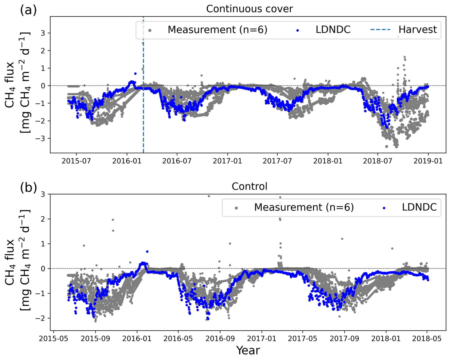
Figure 6 Time series of modeled (blue) CH₄ flux and 6 automatic chamber measurements (gray, n=6) conducted at the (a) continuous cover forestry (CCF) and (b) control stand. Vertical dashed blue line in (a) shows the selective harvest at CCF.

3.4 Ecosystem CO₂ exchange before and after management

The model reproduced pre-harvest NEE more accurately (r=0.88, NSE=0.75, slope=0.92) compared to NEE in either the CCF_Postharvest and RF_Postharvest simulations (Fig. 7a–c). Performance for modeled GPP was similar for both pre-harvest and CCF_postharvest, while RF_postharvest had a lower NSE (0.75) and higher slope (1.26) to the fitted line (Fig. 7d–f). A similar comparison for TER showed that the modeled TER performed well in all three simulations (r=0.94–0.96, NSE=0.87–0.92, Fig. 7g–i).

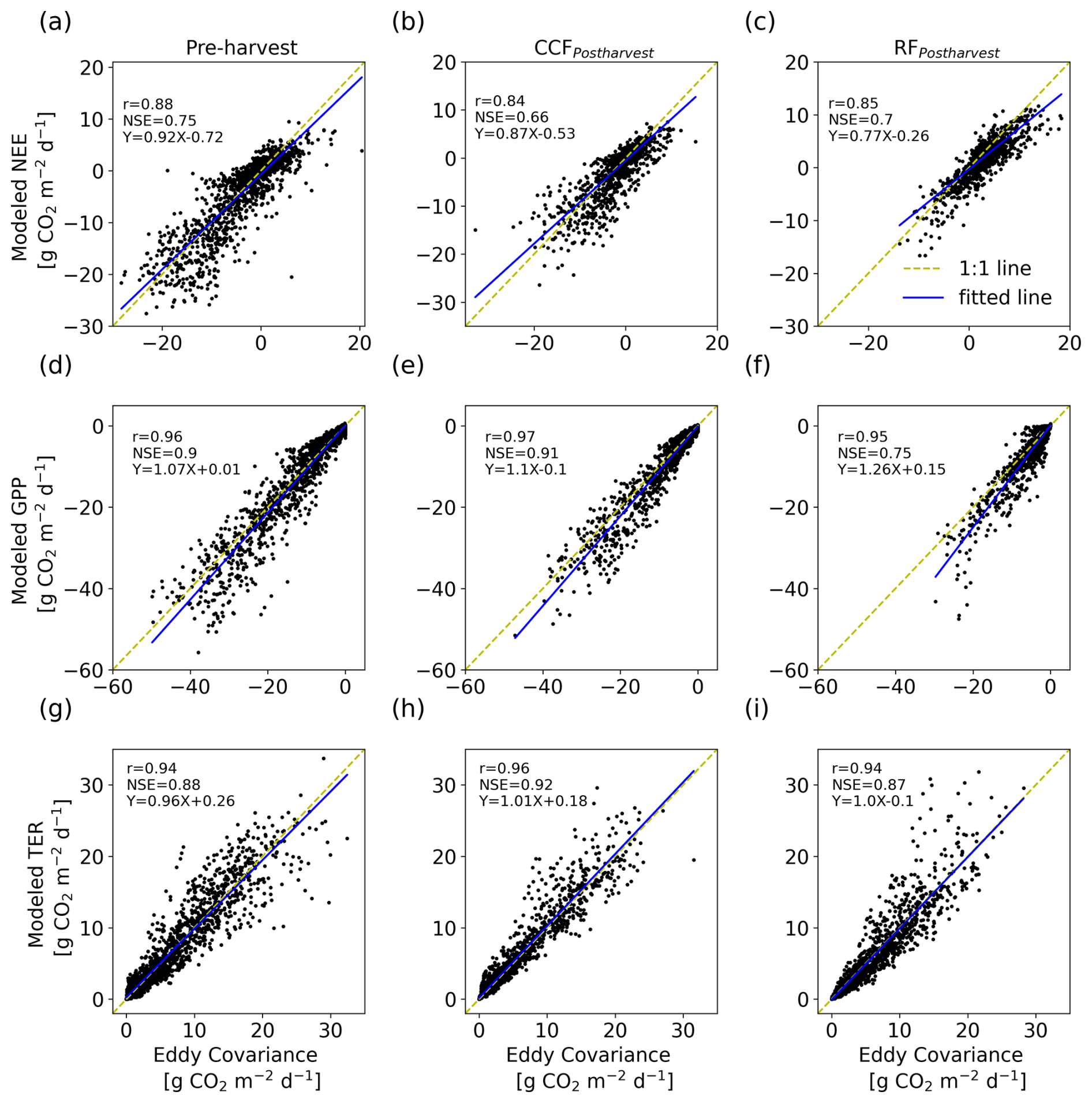
Figure 7 Modeled vs. measured NEE (a–c), GPP (d–f) and TER (g–i) for pre-harvest (a, d, g) and post-harvest conditions of the continuous cover forestry (CCF; b, e, h) and rotation forestry (RF; c, f, i) stand. Correlation coefficients (r) and Nash–Sutcliff model efficiency (NSE) given in the figures show agreement among the variables compared. Yellow dashed lines and blue lines are the 1:1 lines and fitted lines, respectively. The equations for fitted lines are given as Y. To ensure a consistent comparison, periods with missing measurement data were excluded from both the observed and modeled datasets prior to calculating daily sums. As a result, the reported values do not represent complete daily totals. For reference, approximate gap-filled daily time series are presented in Figs. S8, S10, and S12 in the Supplement.

The modeled NEE improved after WT calibration compared with the simulation using the reference WT (Fig. S8a in the Supplement). Overall, the calibrated modeled NEE agreed well with the EC based NEE in both magnitude and temporal dynamics, although some minor discrepancies were evident during pre-harvest period. The highest RMSE for modeled NEE ($\mathrm{9.5}\mathrm{g}{\mathrm{CO}}_{\mathrm{2}}{\mathrm{m}}^{-\mathrm{2}}{\mathrm{d}}^{-\mathrm{1}}$) was in summer 2010 (Fig. S9 in the Supplement). Relatively high RMSE values were also observed during spring, summer and autumn of 2014. The model reproduced the seasonal dynamics of both GPP and TER similarly to the EC-based estimates (Fig. S8b and c in the Supplement, respectively). The largest discrepancy in modeled GPP was observed in summer 2014, when the RMSE was $\mathrm{17.1}\mathrm{g}{\mathrm{CO}}_{\mathrm{2}}{\mathrm{m}}^{-\mathrm{2}}{\mathrm{d}}^{-\mathrm{1}}$ (Fig. S9 in the Supplement). TER was generally simulated well, with the exception of pronounced respiration peaks during the summers of 2010 and 2013. In addition, the model produced slightly higher winter respiration than the EC-based estimates in early 2013 (Fig. S8c in the Supplement). The highest RMSE values for modeled TER were observed during the summers of 2010 and 2014 (Fig. S9 in the Supplement).

Following the selective harvest in 2016, the model reproduced NEE well in 2017, 2020, and 2021. A similar level of agreement was observed during late summer and autumn of 2018 and 2019, although the model simulated greater uptake during spring and early summer in those years (Fig. S10a in the Supplement). In 2016, notable discrepancies in NEE occurred during summer and autumn, coinciding with an overestimation of GPP and an underestimation of TER by the model (Fig. S10b and c in the Supplement, respectively). During spring and early summer of 2018 and 2019, both GPP and TER were overestimated. Summer RMSE values for modeled NEE ranged from approximately 6–8$\mathrm{g}{\mathrm{CO}}_{\mathrm{2}}{\mathrm{m}}^{-\mathrm{2}}{\mathrm{d}}^{-\mathrm{1}}$, whereas RMSE values in the other seasons were generally below 6$\mathrm{g}{\mathrm{CO}}_{\mathrm{2}}{\mathrm{m}}^{-\mathrm{2}}{\mathrm{d}}^{-\mathrm{1}}$ and most often below 4$\mathrm{g}{\mathrm{CO}}_{\mathrm{2}}{\mathrm{m}}^{-\mathrm{2}}{\mathrm{d}}^{-\mathrm{1}}$ (Fig. S11 in the Supplement). The highest RMSE for modeled GPP was observed during summer 2018, while the highest RMSE for modeled TER was observed during summer 2019.

After clear-cutting, modeled NEE captured the gradual transition from a strong daily net CO₂ source during the first three years after harvest to a weaker source, and occasionally even a sink during the summer season, in the following three years (Fig. S12a in the Supplement). Agreement between modeled NEE and the measurements was highest during 2019–2021 and, to a lesser extent, during autumn 2018. From May to August in 2016 and 2017, modeled NEE was underestimated, indicating a smaller net CO₂ source than observed. Modeled GPP agreed well with EC-based GPP during 2016–2019, whereas the model slightly overestimated GPP during late spring and early summer of 2020 and 2021 (Fig. S12b in the Supplement). Similarly modeled TER was lower than EC-based TER during the summers of 2016 and 2017 but was overestimated during late spring and early summer of 2020 and 2021. In contrast, TER in 2018 and 2019 was reproduced well by the model (Fig. S12c in the Supplement). The highest RMSE for modeled GPP and TER was observed in 2021 (Fig. S13 in the Supplement).

On the annual scale, modeled NEE was generally consistent with the EC-based NEE under both pre-harvest and post-harvest conditions, with a few notable exceptions. During pre-harvest period, the largest discrepancy occurred in 2014, followed by 2012 (Fig. 8a), Whereas in both CCF and RF the greatest differences were observed during the first post-harvest year (April 2016–March 2017; Fig. 8b and c). Following selective harvesting modeled NEE indicated that the CCF stand remained a net CO₂ source for the first three years and returned to a net CO₂ sink from the fourth year onward, consistent with EC-based NEE. In the RF stand, both modeled NEE and EC-based NEE indicated that the ecosystem was a net CO₂ source throughout the six post-harvest years following clear-cutting, although annual CO₂ emissions decreased over time.

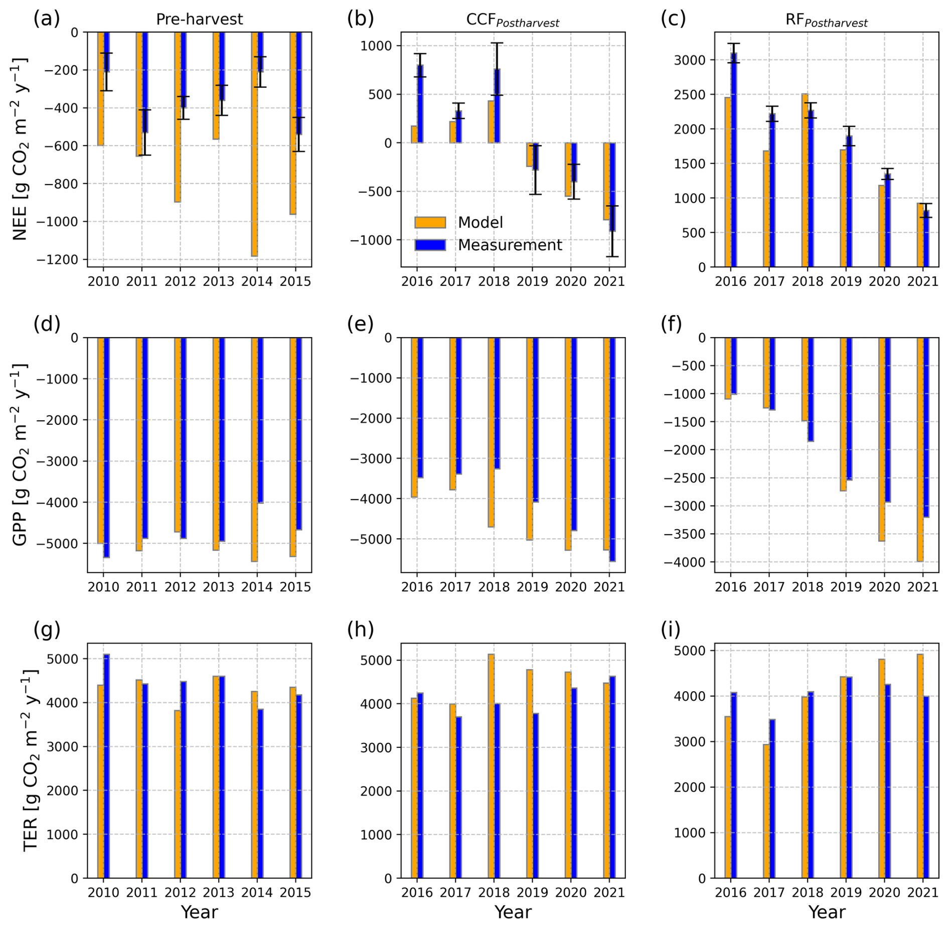
Figure 8 Annual balances of modeled net ecosystem exchange (NEE) and EC-based NEE (gapfilled) for pre-harvest, CCF_postharvest and RF_postharvest shown with the subplots (a), (b), and (c), respectively. The uncertainty estimates for EC-based NEE presented by Korkiakoski et al. (2023), shown with the error bars, were derived following Heimsch et al. (2021) and accounted for both statistical measurement uncertainty and gap-filling error. Pre-harvest, CCF_postharvest and RF_postharvest gross primary product (GPP), are shown in (d), (e), and (f) and total ecosystem respiration (TER), are shown in (g), (h), and (i), respectively. Negative values represent uptake by the ecosystem and positive values represent release of CO₂ to the atmosphere.

During the pre-harvest period, modeled GPP was generally similar in magnitude to EC-based GPP, with the largest discrepancy occurring in 2014 when modeled GPP was 35 % higher (Fig. 8d). In CCF_postharvest, modeled GPP followed a similar temporal pattern to EC-based GPP, although the largest difference was observed in 2018, when modeled GPP exceeded EC-based GPP by 44 % (Fig. 8e). In RF_postharvest, modeled GPP ranged from 21 % lower than EC-based GPP in 2018 to 24 % higher in 2021 (Fig. 8f).

During the pre-harvest period, annual modeled TER was similar to EC-based TER (Fig. 8g). In CCF_postharvest, modeled TER was overestimated by 28 % in 2018 and by 26 % in 2019, while the differences in other years were negligible (Fig. 8h). In RF_postharvest, modeled TER ranged from 16 % lower than EC-based TER in 2017 to 22 % higher in 2021 (Fig. 8i).

3.5 Management effect on soil carbon storage

Following drainage, simulated SC storage showed a continuous decline until the implementation of the management events (Fig. 9). In contrast, the pristine, non-drained peatland exhibited a slight accumulation of SC under the assumption that ground vegetation covered 40 % of the total area. The development of SC after the harvest varied among the managements and depended on the management method. In control, where no trees were removed, SC continued to decrease until the end of the simulation. In CCF, selective harvesting led to a temporary increase in SC, likely driven by carbon inputs from harvest residues. Thereafter, SC began to decline, although it remained higher than in the control throughout the simulation period. In RF, complete tree removal resulted in a temporary increase in SC, again driven by carbon inputs from harvest residues. Although SC began to decrease after several years, it remained higher than in both the control and CCF simulations. Annual SC loss for 2010–2015 was 233 $\mathrm{g}\mathrm{C}{\mathrm{m}}^{-\mathrm{2}}{\mathrm{yr}}^{-\mathrm{1}}$. SC loss for the period of March 2016–2021 was 221 $\mathrm{g}\mathrm{C}{\mathrm{m}}^{-\mathrm{2}}{\mathrm{yr}}^{-\mathrm{1}}$ in control, 95 $\mathrm{g}\mathrm{C}{\mathrm{m}}^{-\mathrm{2}}{\mathrm{yr}}^{-\mathrm{1}}$ in CCF, and SC gain 79 $\mathrm{g}\mathrm{C}{\mathrm{m}}^{-\mathrm{2}}{\mathrm{yr}}^{-\mathrm{1}}$ in RF.

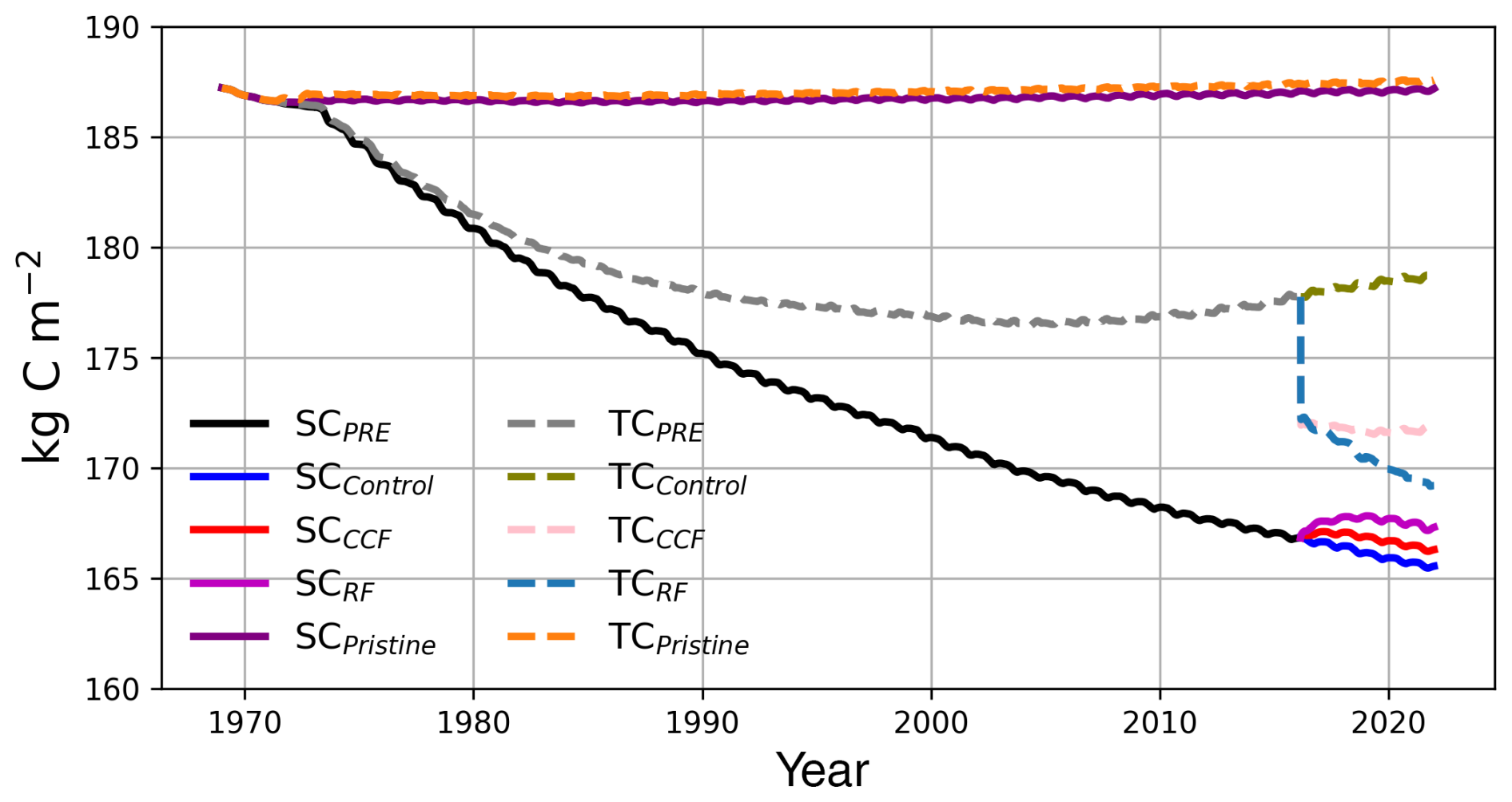
Figure 9 Modeled soil carbon (SC, solid lines) and total carbon (TC, dashed lines) time series for the different simulations from 1969 to 2021. Non-drained pristine peatland SC and TC are represented by purple and orange lines, respectively. Black and gray lines show the SC and TC development up to the harvest event in March 2016, respectively. Blue, red, and magenta lines represent SC development for the control, post-harvest CCF, and post-harvest RF simulations, respectively. Olive green, pink, and light blue lines represent TC development for the control, post-harvest CCF, and post-harvest RF simulations, respectively.

The small difference between total carbon (TC) and SC in the pristine peatland was due to the relatively low carbon storage in vegetation (Fig. 9). Following drainage, TC declined across all forestry simulation scenarios, as soil carbon losses were greater than the carbon sequestered by vegetation. Continued forest growth led to greater carbon accumulation in tree biomass, resulting in a stabilization of TC between 2000–2010 and an increase thereafter as carbon uptake by vegetation exceeded soil carbon loss. In control, TC continued to increase until the end of the simulation. However, in CCF, TC decreased for a few years after the selective harvest and once the remaining vegetation rebounded TC started to increase again. In contrast, in RF, the accumulation of carbon by the forest stopped after the mature forest had been removed. Furthermore, carbon accumulation in the newly established stand was insufficient to compensate for soil carbon losses, leading to a continued decrease in TC.

The litter pool comprising soluble compounds (solutes), which has a rapid turnover rate, received a large input immediately after harvest but declined rapidly thereafter (Fig. 10a). Following this initial increase, solute levels in RF were even lower than those in the control and CCF during 2016–2019, as the remaining vegetation contributed little fresh litter input. However, solute inputs increased again from the fourth year after clear-cutting as the regenerating birch stand began contributing litter. In both CCF and RF, cellulose and lignin pools dominated total litter storage after harvest, whereas the contribution of solutes remained relatively small (Fig. 10b and c). The cellulose pool reached its maximum in the third year after harvest in RF and the second year in CCF before beginning to decline. In contrast, the lignin pool remained elevated during the first three post-harvest years and began to decline in the fourth year after harvest.

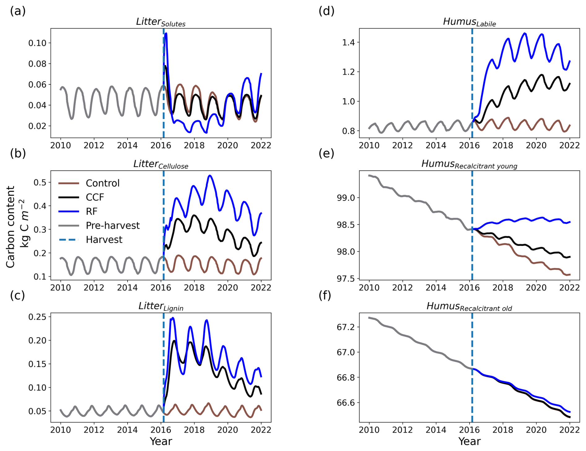
Figure 10 Dynamics of litter (a–c) and humus (d–f) pools during the pre-harvest and post-harvest periods. Gray lines represent the pre-harvest period, brown the control, black Continuous Cover Forestry (CCF), and blue Rotation Forestry (RF). The dashed light-blue line denotes the harvest event.

In the new model version, a larger fraction of carbon entering the humus pools was allocated to the recalcitrant young pool (Fig. 10e) than in the previous version (Fig. S15 in the Supplement). Consequently, heterotrophic respiration increased in the new model version (Fig. S16 in the Supplement) because the larger recalcitrant young pool decomposed more rapidly. Following management, inputs from decomposing harvest residues also caused an initial increase in the storage of the fast-decomposing labile humus pool (Fig. 10d). This effect was stronger in RF than in CCF because of the greater harvest-residue input. The labile humus pool reached its peak earlier in RF than in CCF. Decomposed harvest residues also contributed to an increase in the recalcitrant young humus pool (Fig. 10e), whereas only minor effects were observed in the recalcitrant old humus pool after harvest (Fig. 10f).

4 Discussion

The process-based model LandscapeDNDC accurately reproduced the observed forest structure of the drained forested peatland before and after the management events when driven by the prescribed species composition. The simulated LAI of the mature forest was similar to the field-estimated LAI reported by Leppä et al. (2020) for the same site. The combined LAI of the three simulated tree species (Pine, Spruce, and Birch) varied seasonally between 2–4 m² m⁻², which is within the range reported by Rautiainen et al. (2012) for mixed forests in southern Finland. However, the combined modeled LAI of all tree species did not correspond well to the satellite-estimated LAI at the site. This discrepancy could arise because the satellite-estimated LAI likely reflects mainly the upper canopy, which at the study site consisted predominantly of pine and birch trees. Given the dense canopy of the control stand (Fig. A1), the contribution of secondary vegetation and forest floor may have been only partially captured by the satellite observations.

Good agreement between modeled and satellite-estimated LAI was observed in the CCF and RF stands after management. This was likely due to the sparse vegetation cover in the CCF stand following selective harvest and the near absence of vegetation in the RF stand after clear-cut (Fig. A1). Therefore, the comparison between modeled and satellite-estimated LAI in these sparsely vegetated stands provides a more accurate picture of stand-level LAI. Furthermore, the declining trend in the modeled LAI of pine and spruce in control stand may have resulted from the competition between species in the model, as well as the allocation of available nutrients among species.

The model exhibited a tendency to conserve water during the 2018 drought, potentially due to interactions between vegetation and soil moisture processes. Furthermore, the saturated hydraulic conductivity and the vanGenuchten parameters used to parameterize the soil water retention curve may have constrained soil water content from declining below a certain level. Nevertheless, a comprehensive analysis of extreme drought episodes is outside the scope of this study, which focuses forest development under different management regimes under typical climate conditions.

Although simulations driven by site-measured WT were possible with LandscapeDNDC, the implementation of a dynamic WT approach in this study enables the model to generate WT internally, thereby improving its applicability to peatland ecosystems. The model successfully captured the more pronounced WT fluctuations induced by management in the RF simulation. However, management-induced WT fluctuations were less evident in the CCF stand immediately after harvesting; nevertheless, the simulated WT agreed well with the measured WT from the third year onward. Previous field studies at the Lettosuo site reported management-induced WT fluctuations, including a WT rise of 18–23 cm in the RF stand after clear-cutting (Leppä et al., 2020; Korkiakoski et al., 2019, 2020), consistent with the trends simulated in this study.

The model simulated CH₄ fluxes well in both the control and CCF stands, and the site acted predominantly as a CH₄ sink. The simulation indicated that CH₄ uptake in the CCF stand was, on average, 17 % lower than in the control stand during the five years following selective harvesting. A reduction in CH₄ uptake following selective harvest has also been observed in drained peatland (Korkiakoski et al., 2020) and upland boreal forest (Sundqvist et al., 2014). Additionally, we investigated the autumn mismatch in CH₄ fluxes by modifying the CH₄ oxidation and production parameters. Although reducing CH₄ oxidation shifted the simulated flux from a stronger to a weaker CH₄ sink, and increasing oxidation had the opposite effect, these parameter adjustments did not resolve the mismatch between the simulated and observed fluxes. The simulated CH₄ fluxes were considered satisfactory because they fell within the range of fluxes observed in chamber measurements. The minor differences between the modeled and observed CH₄ fluxes may be attributed to spatial heterogeneity not fully represented in the model. The chamber plots varied in species composition and abundance, potentially affecting CH₄ transport from the soil to the atmosphere. In contrast, the model used a simplified representation of vegetation consisting of ground vegetation and three tree species. In addition, variations in soil moisture, water table depth, and soil temperature among individual chamber locations could have influenced the measured CH₄ fluxes. Together, these factors may have contributed to the observed minor discrepancies between simulations and measurements.

Following clear-cutting, CH₄ flux dynamics in the RF were sensitive to changes in the WT. According to the measurements, the RF shifted from a CH₄ sink to a source after clear-cutting (Korkiakoski et al., 2019). In contrast, the model predicted the RF to remain a CH₄ sink under low-WT conditions, while under high-WT conditions RF was either a CH₄ source or sink depending on the season. Another study conducted at two RF sites found that both sites remained small CH₄ sinks (0.07 and 0.52 $\mathrm{mg}{\mathrm{CH}}_{\mathrm{4}}{\mathrm{m}}^{-\mathrm{2}}{\mathrm{d}}^{-\mathrm{1}}$) after clear-cutting (Huttunen et al., 2003). Differences in CH₄ fluxes could be attributed to spatial variability in the WT. Thus, chamber location relative to the ditch is an important consideration when comparing model results with measurements (e.g. Laurén et al., 2021). In this study, the manual chambers were situated 4–22.5 m from the ditch, an average WT from the chamber locations was used in the analysis. Logger-based WT measurements were also included to account for spatial variability across site.

The simulated annual CO₂ balances showed a net CO₂ sink during the pre-harvest period, consistent with the observations. Similarly, the simulations for CCF_postharvest and RF_postharvest reproduced the observed post-harvest dynamics, accurately capturing both the timing of the transition of the CCF stand back to a CO₂ sink after harvest and the duration for which the RF stand remained a CO₂ source.

In RF, the ecosystem became a net CO₂ source largely due to the loss of tree assimilation capacity and increased respiration from harvest residues (Korkiakoski et al., 2019). The model underestimated NEE during the first two years after clear-cutting because simulated TER was lower than observed. The higher simulated GPP in 2020 and 2021 was related to the introduction of birch seedlings in 2019. In the model, newly introduced seedlings are assigned a minimum diameter of 1 cm at breast height and seedling height of 50 cm, which may result in larger birch seedlings than those observed in the field during the early establishment phase. Consequently, simulated GPP was likely overestimated in 2020 and 2021. In addition, lower self-thinning rates may have contributed to the elevated initial GPP after birch reintroduction (Forrester et al., 2021). Therefore, using fewer seedlings than observed may improve the simulation of early post harvest GPP. Indeed, a test simulation with approximately 11 000 birch seedlings, instead of 17 000, produced GPP values that were closer to the observation-based estimates.

In CCF following selective harvesting, the ecosystem acted as a CO₂ source during the first three years and as a sink during the subsequent three years. However, the model indicated a slight increase in GPP and TER already in the third year after harvest, a trend that was not evident in the observation-based estimates. This suggests that the model may overestimate the recovery rate of vegetation after harvesting. In addition, the simulated WT could not fall below the reference WT (Z_gw) of 0.62 m, potentially preventing drought stress from affecting tree growth in the simulations. Because water remained available for root uptake throughtout the simulation period. The model did not capture the effects of the summer 2018 drought on the CO₂ balance that were reported by Korkiakoski et al. (2023) when examining daily time series. Nevertheless, discrepancies between simulated and observed annual CO₂ balances in 2018 were small for both CCF and RF, despite the exceptionally dry conditions that year (Lehtonen and Pirinen, 2019). This suggests that water availability below Z_gw had only a minor influence on the annual CO₂ balance.

In this study, the simulated annual soil carbon (SC) loss was 421 $\mathrm{g}\mathrm{C}{\mathrm{m}}^{-\mathrm{2}}{\mathrm{yr}}^{-\mathrm{1}}$ over the 30-years period from 1980 to 2009. Using 37 peatland sites representing different fertility classes across Finland, Simola et al. (2012) reported minimum carbon losses from drained peat soils of approximately 150 $\mathrm{g}\mathrm{C}{\mathrm{m}}^{-\mathrm{2}}{\mathrm{yr}}^{-\mathrm{1}}$. At fertile drained peatland sites in southern Finland, SC losses can reach approximately 1000 $\mathrm{g}\mathrm{C}{\mathrm{m}}^{-\mathrm{2}}{\mathrm{yr}}^{-\mathrm{1}}$ (Ojanen et al., 2013). The study site considered here is a MtkgII type peatland forest (Vasander and Laine, 2008). Among drained MtkgII peatland sites, peat carbon loss can vary considerably depending on WT and temperature conditions (Ojanen et al., 2013). Therefore, the simulated SC loss falls within the range reported in the literatures.

The slower decline in SC storage in CCF and the temporary increase in SC storage in RF, compared with the continuous SC loss in the control simulation, were primarily driven by increased carbon inputs from fresh litter and harvest residues. Because residue inputs were larger in RF than in CCF, SC storage increased more in RF. The higher WT in RF may also have reduced decomposition rates and thereby contributed to greater soil carbon retention. However, SC storage began to decline again from the fourth year after harvesting in RF and even earlier in CCF as the contribution of decomposing harvest residues diminished. In addition, increasing vegetation growth enhanced transpiration and lowered the WT, further promoting soil carbon loss.

Overall, the model successfully captured the transition of a mature forest stand to stands managed under CCF and RF. The simulated annual CO₂ balances indicated a faster transition from a source to sink in CCF than in RF, consistent with observations (Korkiakoski et al., 2023). The CH₄ sink strength was lower in CCF than in the control stand, while CH₄ flux in RF showed a stronger sensitivity to changes in WT. Following harvest, WT responded more rapidly in RF than in CCF, although the simulated WT for both management regimes agreed well with the measurements during the later post-harvest years. The simulated LAI fluctuations in the mature forest are likely related to species competition and nutrient allocation among species within the model and could be investigated further in future studies. The model's tendency to conserve water during drought periods, and the resulting effects on the simulated CO₂ balance requires future considerations. In addition, vegetation heterogeneity within the chamber footprints should be considered when comparing CH₄ fluxes from chamber measurements with modeled fluxes.

The model was originally developed for mineral soils, and modifications to carbon allocation among humus pools were therefore required to represent peatland characteristics. Using the original mineral-soil parameterization resulted in unrealistically low soil respiration because a large proportion of carbon was allocated to the recalcitrant old pool. In the revised implementation, a greater fraction of carbon was directed to the recalcitrant young humus pool, which has a higher turnover rate than the recalcitrant old pool. Consequently, decomposition rates increased, leading to higher soil respiration and a more realistic representation of peat decomposition.

The simulations were initialized from the onset of drainage in 1969 and continued until stand maturity to capture long term development of tree growth and soil carbon stocks. This long-term simulation approach was intended to ensure that the model can also be applied to future scenario analyses. Although such analyses were beyond the scope of the present study, the model provides a useful framework for investigating future forest management strategies, carbon dynamics, and water balance in drained peatland forests.

5 Conclusions

The process-based LandscapeDNDC model was successfully applied to simulate forest development under different managements on drained peatland from seedlings to maturity. The simulations demonstrated that estimates of carbon fluxes and the overall greenhouse gas balance vary substantially depending on management type, underscoring the importance of detailed information on management history, tree dimensions, and regrowth dynamics. The model reproduced measurement-derived NEE, GPP and TER both before and after harvest, while also capturing changes in forest structure. The implementation of a new dynamic water table (WT) module improved simulations of WT level, soil moisture, peat decomposition, and CH₄ fluxes, thereby enhancing the representation of carbon dynamics. We were able to illustrate the contributions of harvest residue to litter and humus pool and their decomposition. This successful application of LandscapeDNDC provides a robust basis for investigating future management scenarios in drained peatland forests, with respect to both carbon and energy balances. The model therefore offers valuable insights for developing forest management strategies that supports climate neutrality in peatland ecosystems.

Appendix A:  

A1 Lettosuo site

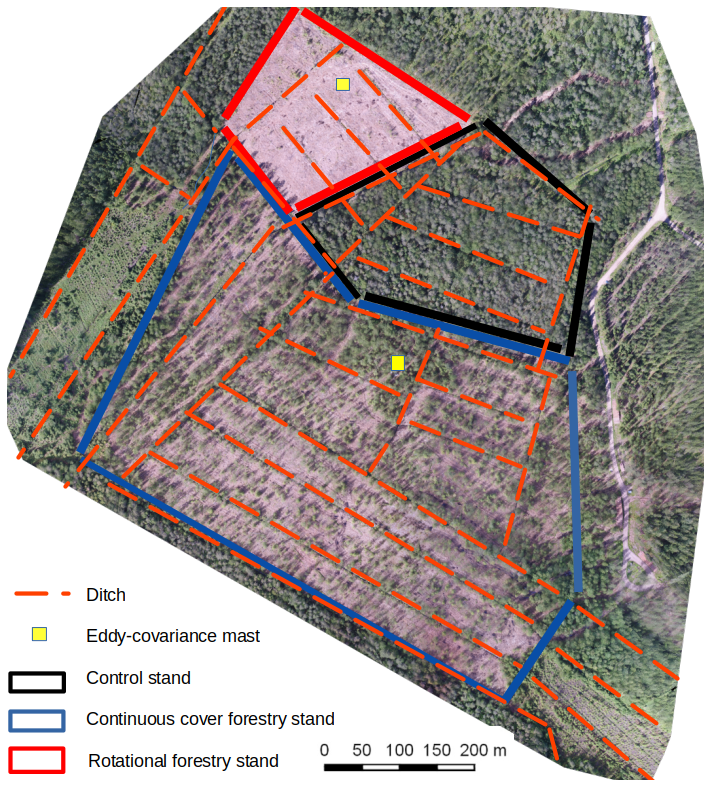
Figure A1 Aerial view of the Lettosuo site in August 2016. Black, blue, and red boxes indicate the control, Continuous Cover Forestry (CCF), and Rotational Forestry (RF) stands, respectively. Yellow squares show the eddy-covariance mast locations, and orange dashed lines show the ditch network.

A2 Sensitivity test

Table A1 Sets of soil parameters (unitless) used in sensitivity test for soil processes (MeTr^x module).

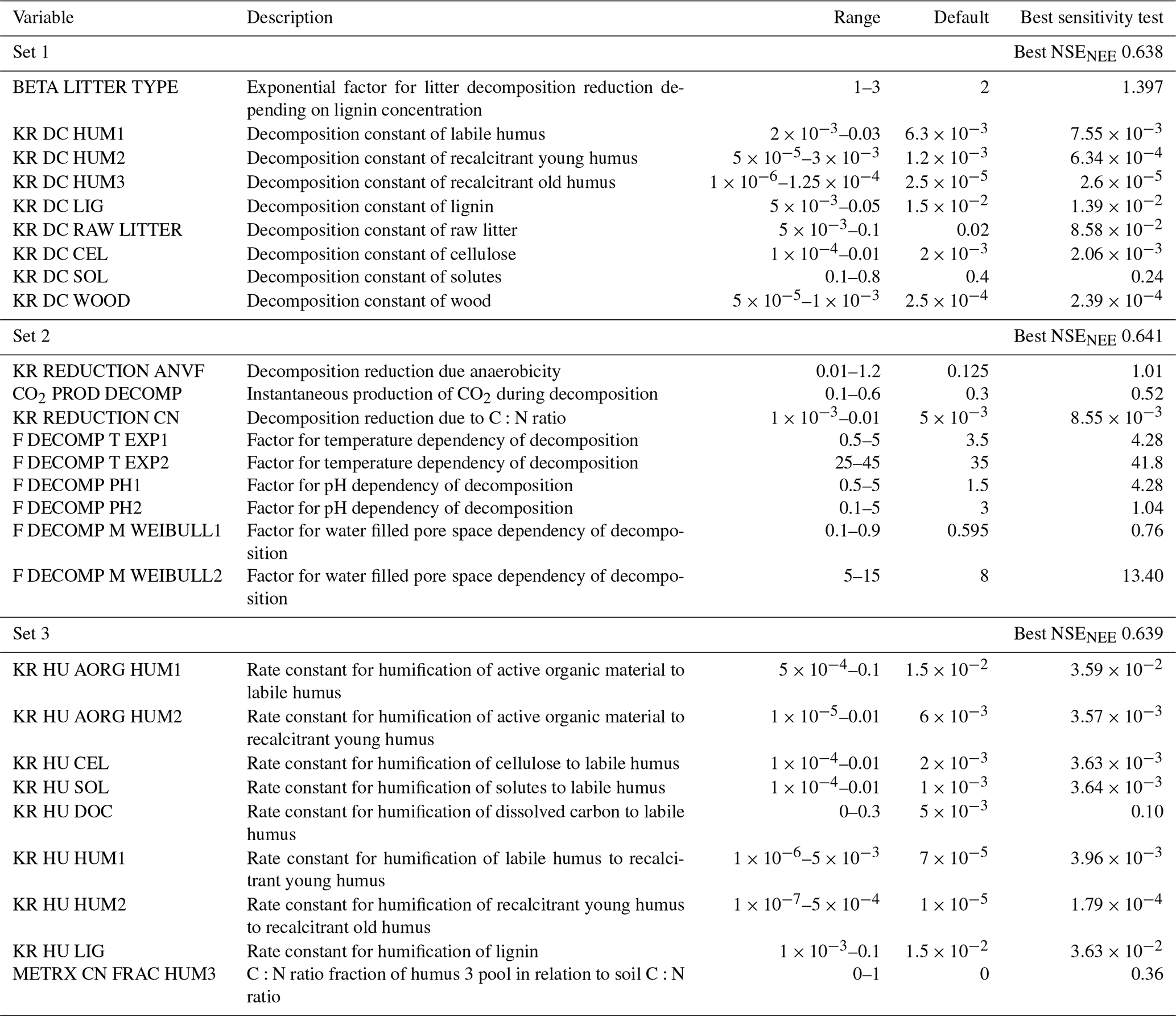
Table A2 Species parameters used in running both the sensitivity tests and full forest runs. These remained constant unlike the soil parameters for sensitivity tests in Table A1.

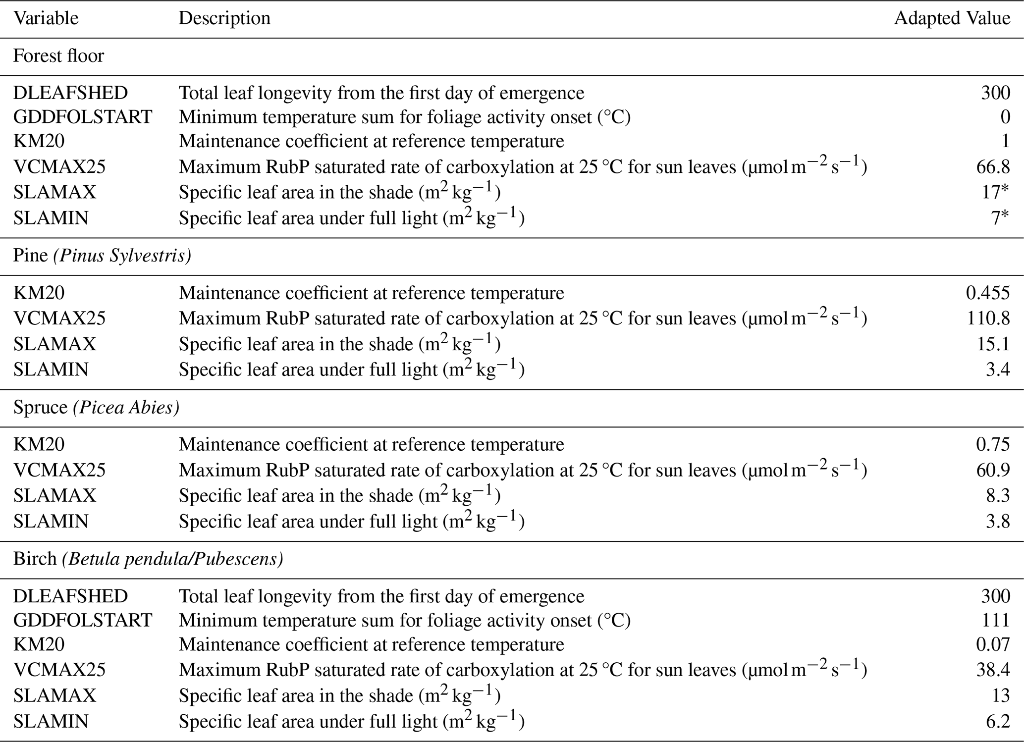
^* 17 for pristine.

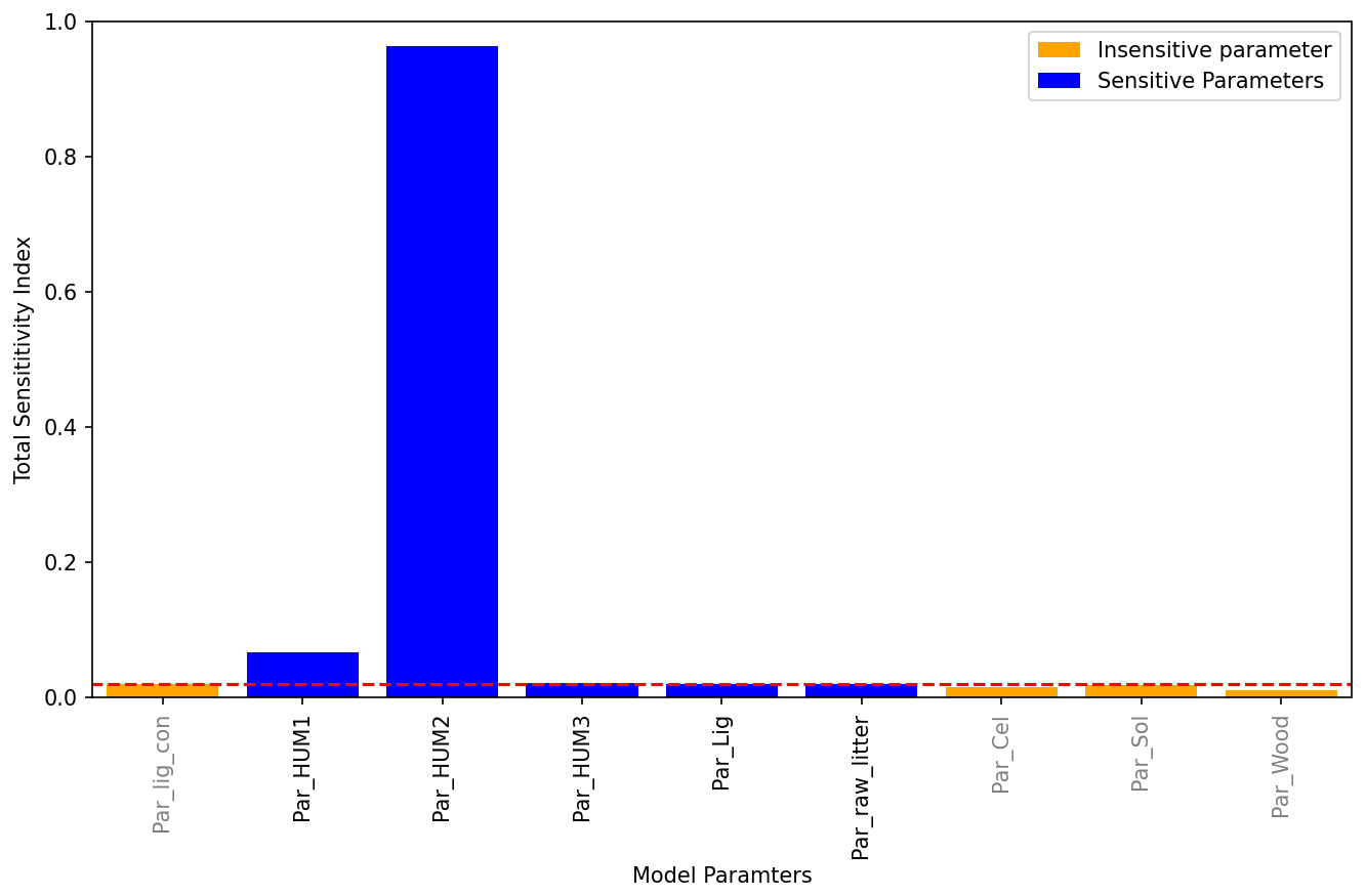
Figure A2 Sensitivity analysis results for the first parameter set. Black x-ticks denote the five most sensitive parameters identified by the FAST algorithm, and the red dashed line indicates the sensitivity threshold defined by the fifth-ranked parameter. Grey x-ticks represent parameters classified as non-sensitive. The threshold depends on the user-defined number of sensitive parameters included in the analysis.

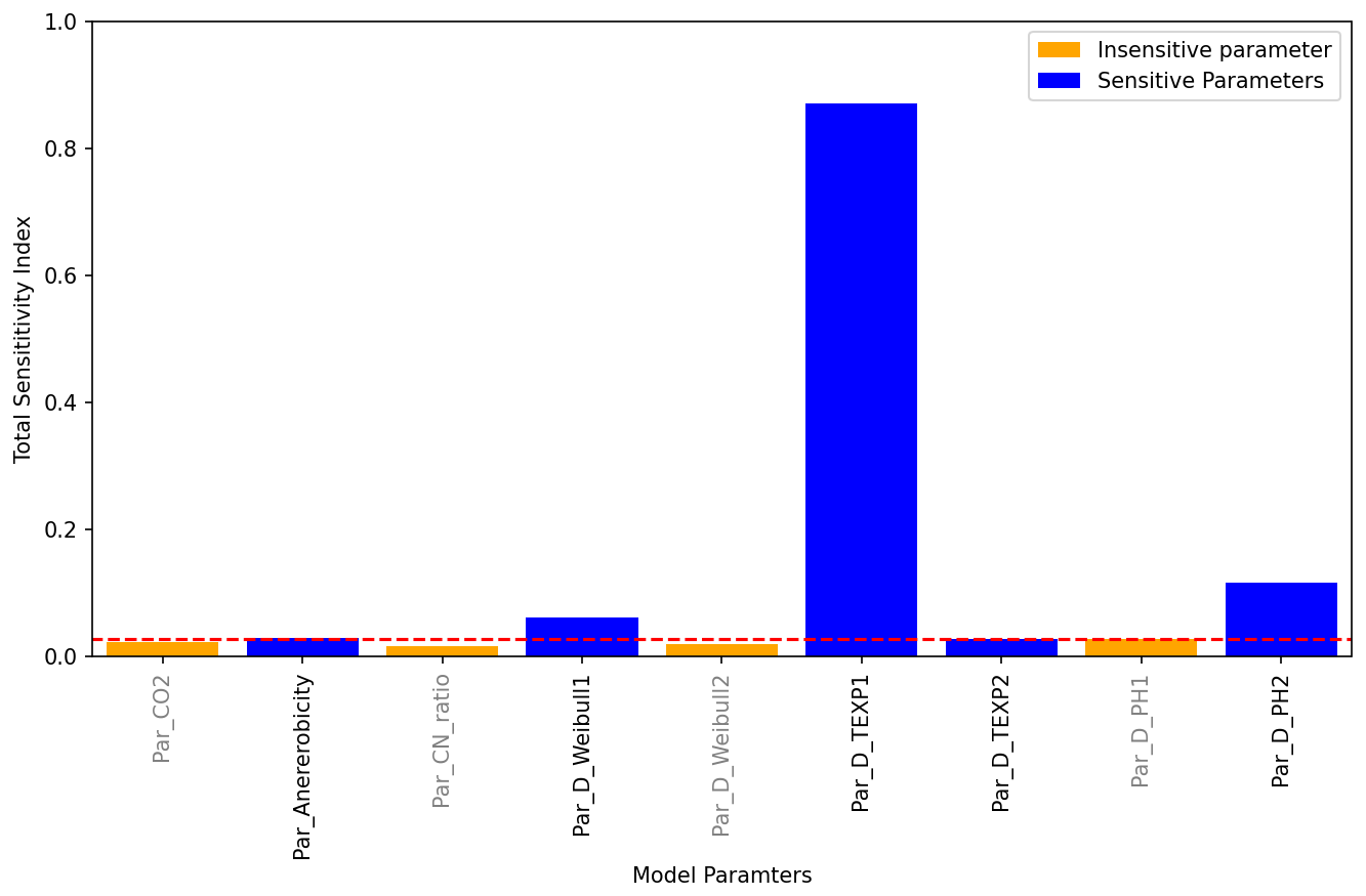
Figure A3 Sensitivity analysis results for the second parameter set. Black x-ticks indicate the five most sensitive parameters identified by the FAST algorithm, and the red dashed line marks the threshold in the total sensitivity index corresponding to the fifth most sensitive parameter. Grey x-ticks indicate parameters classified as non-sensitive by the FAST algorithm.

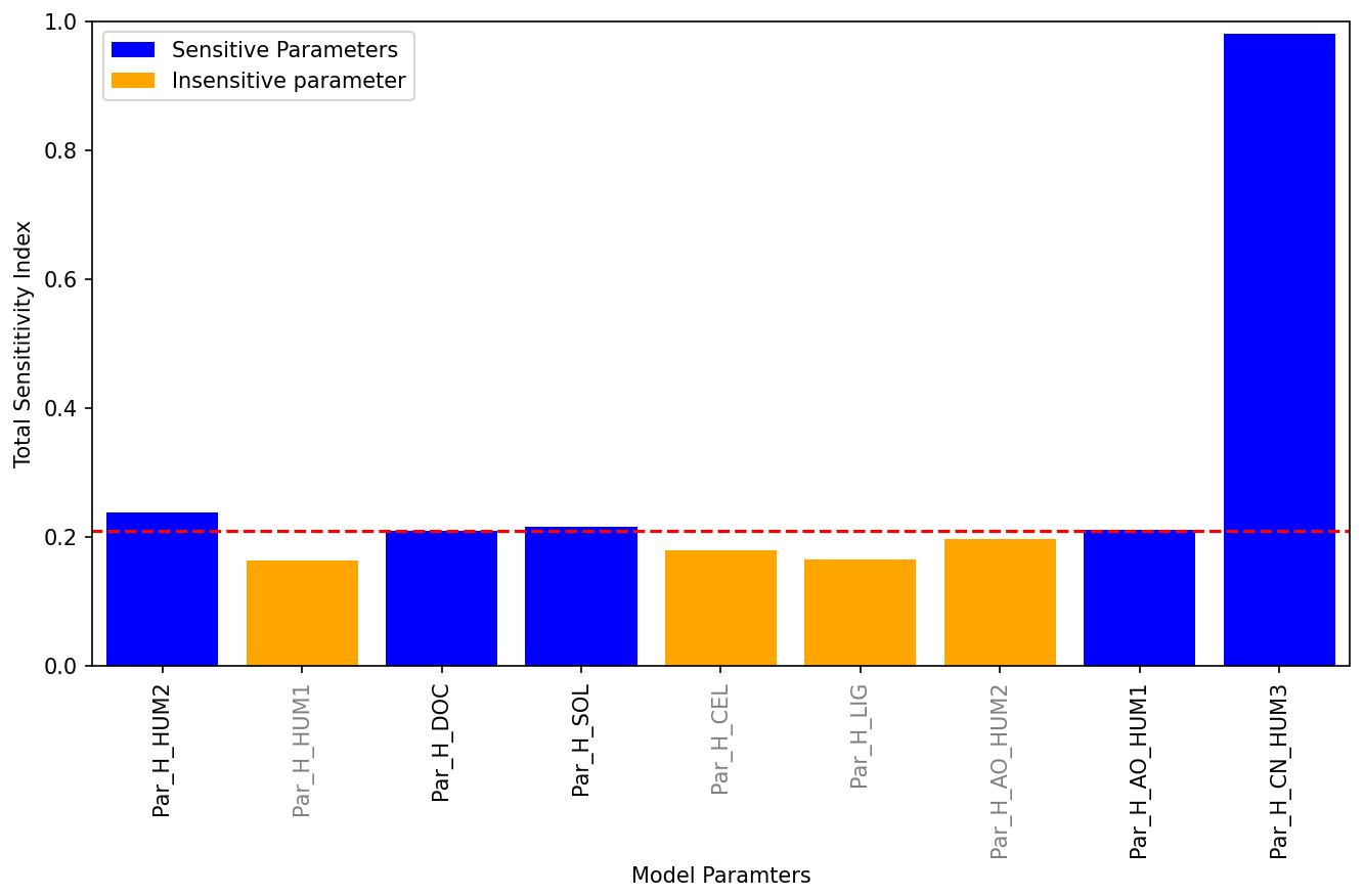
Figure A4 Sensitivity analysis results for the third parameter set. Black x-ticks indicate the five most sensitive parameters identified by the FAST algorithm, and the red dashed line marks the threshold in the total sensitivity index corresponding to the fifth most sensitive parameter. Grey x-ticks indicate parameters classified as non-sensitive by the FAST algorithm.

A3 Full forest simulations

Table A3 Soil parameters (unitless unless stated) used in running the full forest simulations and their associated values.