Modeling of radiative transfer through cryospheric Earth system: software package SCIATRAN

The cryosphere plays a crucial role in global climate change. To accurately quantify impacts of typical cryospheric surface types, such as snow, ice, and melt ponds on the radiative processes both in the atmosphere and at the surface, new developments in the radiative transfer modeling are necessary. This paper summarizes recent developments in the coupled atmosphere-snow(water)-ice-water radiative transfer model SCIATRAN, which are essential for cryospheric science applications. Novel implementations include a polarized treatment of the coupled ocean-atmosphere, support for multi-layer ice with an ice crust, a flexible interface for incorporating diverse total suspended matter, and an improved cloud parameter input for mixed clouds. We also introduce new surface reflection models and expanded databases of inherent optical properties for snow and ice. Furthermore, it includes selected verification and validation results obtained by comparing SCIATRAN simulations with benchmark data and with measurements from various campaigns.

The SCIATRAN software package is freely distributed via the homepage of the Institute of Environmental Physics (IUP), University of Bremen: https://www.iup.uni-bremen.de/sciatran/ (last access: 23 June 2026.

1 Introduction

Global warming is causing extensive shrinking of the cryosphere (IPCC, 2019), which is threatening the achievements of global sustainable development goals due to the associated rise in sea levels (IPCC, 2021). To gain a thorough understanding of the changing cryosphere, both in the past and present as well as in the future, accurate quantification of the coverage and properties of snow, ice, and melt ponds (SIM) is essential (Wendisch et al., 2018, 2023). The necessary data are provided by campaign-based, aircraft, and satellite observations. Observed changes of cryospheric characteristics can be used by climate models to predict their impact and provide valuable knowledge for elaborating risk reduction strategy.

To determine characteristics of the cryosphere from observations, processes related to the light propagation in the cryosphere and interaction between the cryosphere and the atmosphere need to be included in radiative transfer models (RTMs), see e.g. Mei et al. (2023). In particular, developments in surface models employed by RTMs are essential. For measurement campaigns, development of RTMs and designing of new instruments and measurement setups are closely related. On the one hand, implementing new capabilities in the models helps to extend the variety of the measured quantities and interpret measurement data. On the other hand, the measured data help to validate and improve RTMs. For the interpretation of aircraft and satellite observations, RTMs are fundamental tools to understand the sensitivity of observations to various cryospheric parameters and to design retrieval algorithms. This means that the development of appropriate RTMs is one of the key aspects of obtaining reliable observational data. A significant interest in estimating SIM parameters and, thus, an urgent need for the development of RTMs, which are capable of handling these parameters, is illustrated by a rapid increase of the number of scientific publications on the topics of “snow, ice, melt ponds” and “radiative transfer” during the last decades, see Fig. 1.

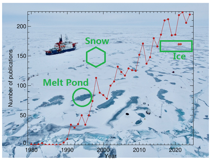
Figure 1 Number of publications on the topics of “snow, ice, melt ponds” and “radiative transfer” between 1980 and 2020. The background picture was provided by Dr. G. Spreen from the University of Bremen.

In recent years, machine learning (ML) approach moved into the focus in the cryospheric community. This technique relies on training datasets, which are either simulated using an RTM or retrieved from measurements. The latter process also requires a suitable RTM. Thus in a long term term perspective, development of RTMs will be essential not only for classical physical-based retrievals but also for ML-based methods.

Research studies related to the cryosphere typically focus on the coverage by SIM and thier reflective characteristics. The latter are determined by SIM properties, e.g. for snow by its grain size, particle shape, density, and depth (Jin et al., 2008; Picard et al., 2009; Mei et al., 2021a, b; Pohl et al., 2020b). Most commonly, the surface reflectivity is described by a Lambertian albedo, which is estimated using the delta-Eddington, two-stream, or asymptotic methods (Wiscombe and Warren, 1980; Flanner et al., 2007; Malinka et al., 2016, 2018). As discussed by Mei et al. (2020b, 2021a, b), an inability of many SIM surface reflectance models to adequately describe directional reflection properties of the surface, i.e. its Bidirectional Reflectance Distribution Function (BRDF), limits our ability to obtain reliable estimations of surface and atmospheric parameters over the cryosphere. More sophisticated reflection models are also needed to consider inhomogeneous observation scenes whose reflective properties are determined e.g. by a mixture of snow, ice, and melt ponds.

The most general approach to consider a SIM layer within RTM is to include its optical properties into the radiative transfer equation (RTE) for a coupled atmosphere-ocean (CAO) system. There are several techniques available to solve RTE for a CAO system. A brief overview of the models published until 2019 is presented by Chowdhary et al. (2019). In Chowdhary et al. (2020) CAO RTMs were used to generate Stokes vector components I, Q, and U of the upwelling radiance just above a rough ocean surface and at the top of the atmosphere. Although almost every CAO RTM can be modified to calculate radiative transfer through a SIM layer, various technical issues need to be dealt with. To our knowledge, there are a few similar models, namely, CASIO-DISORT (Hamre et al., 2004), COART (Jin et al., 2006) and AccuRT (Stamnes et al., 2018), both based on the discrete-ordinates technique (Stamnes et al., 1988), where such modifications were undertaken.

In this study, we present an implementation of a SIM layer in the coupled atmosphere-ocean mode of SCIATRAN RTM. To represent the inherent optical properties of a snow layer, one of the two methods implemented in SCIATRAN can be selected. The first one, previously explored in e.g. Langlois et al. (2020) and Mei et al. (2021a, b), assumes the layer to consist of ice crystals with a particular shape and size. Selecting the Snow Particle Shape (SPS), Snow Grain Size (SGS) and snow density, the optical properties of a snow layer are computed using the scattering theory of electromagnetic waves, see Baum et al. (2011), Yang et al. (2013) and related works for details. The second approach represents a snow layer as a random mixture of irregular ice grains and air gaps. In this case, the stereological method and geometrical optics provide the foundation for deriving analytical formulas to calculate the optical properties of the mixture, see Malinka (2014, 2015) and related studies for details.

For an ice layer, the SCIATRAN model considers scattering and absorption processes within the ice accounting for contaminants such as yellow substance (e.g. Chromophoric Dissolved Organic Matter, CDOM) and algae. A surface heterogeneity can also be accounted for. In addition, SCIATRAN is able to account for a scattering layer of white ice, which can significantly affect the radiative transfer through the ice layer.

Melt ponds on sea ice are represented in SCIATRAN by a multi-layer system whose directional reflectance is determined by the pond depth, geometrical thickness of the ice below the water, and inherent optical properties of the water and interior ice. A thin ice layer on top of the melt pond can also be introduced. Thus, reflectance for both open (with no skim ice) and frozen-over (with a skim of ice) ponds, as observed e.g. by Malinka et al. (2018), can be calculated.

The paper is structured as follows: Sect. 2 presents the theoretical background of the radiative transfer through the cryospheric earth system, including both coupled and decoupled ocean-atmosphere models. In Sect. 3, we discuss the inherent optical properties of snow and ice that are available in the SCIATRAN software package. Section 4 presents verification results of the software based on comparisons between the SCIATRAN simulations and other radiative transfer models. In Sect. 5, we show the comparison of SCIATRAN predictions with campaign-based measurements. Finally, Sect. 6 provides the conclusions.

2 RT problem and boundary conditions for the cryospheric Earth system

Throughout this paper, the term “radiative transfer through the cryospheric Earth system” refers to the processes of radiative transfer through two adjacent horizontally homogeneous media. In the current version of SCIATRAN, the upper medium comprises an air layer, which might be bounded by a snow layer from below, while the lower medium consists of liquid water and ice layers (multiple layers are possible). In this paper, the upper and lower medium will be referred to as the atmosphere and the ocean, respectively. A typical example of the lower medium is melt ponds on the sea ice. They can either be open or frozen having a thin layer of ice on top of the water. Each medium can be divided into several adjacent sub-layers enabling us to assume a vertical inhomogeneity of optical parameters within each particular sub-layer.

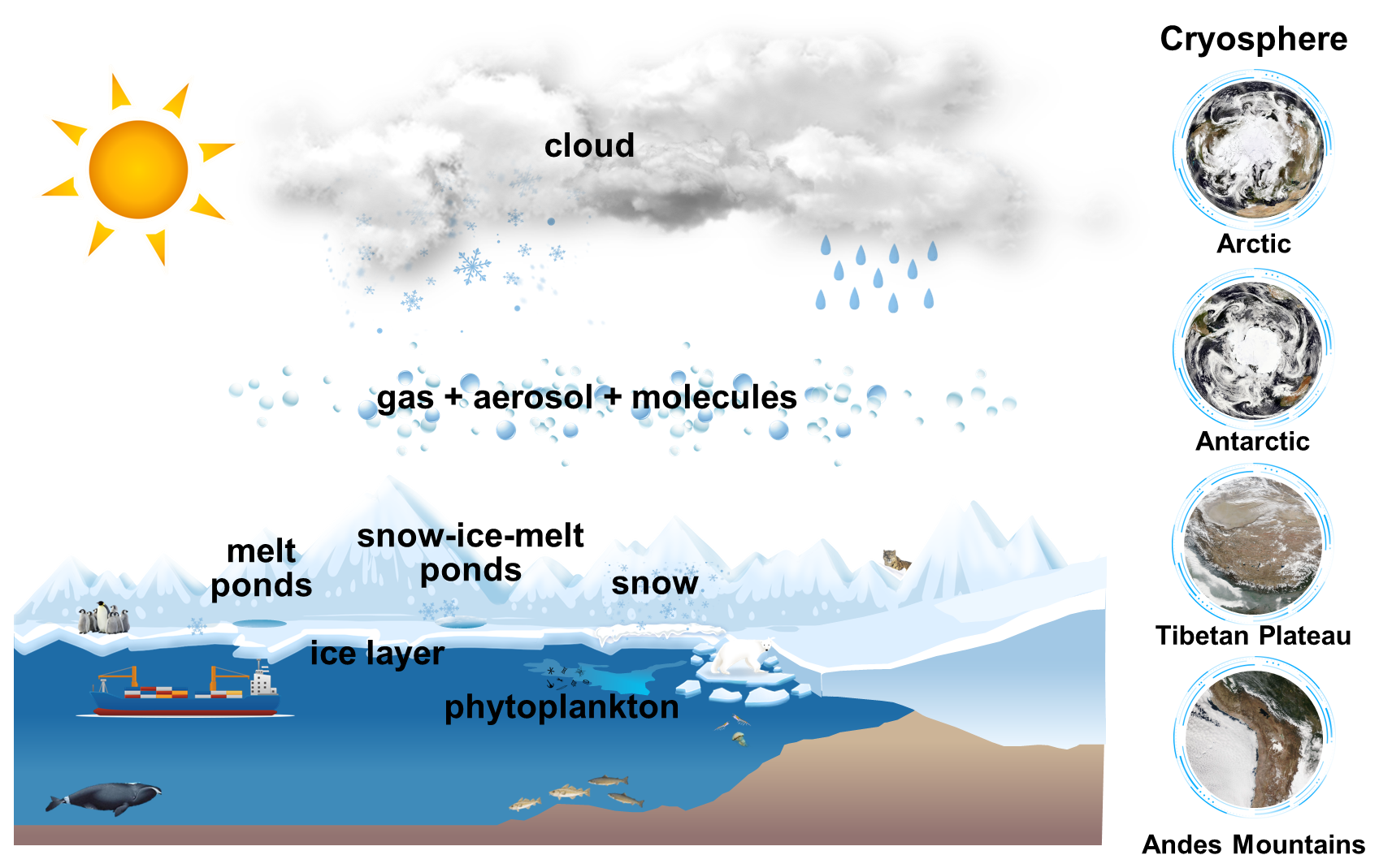
Figure 2 Schematic figure of the cryospheric Earth system discussed in this paper. The figures on the right showing Arctic, Antarctic, the Tibetan Plateau and the Andes Mountains are the NASA Black Marble products.

In both media various radiative transfer processes are taken into account. In the atmosphere, the absorption and scattering of radiation by gas molecules, aerosol, ice particles or water droplets within clouds and ice crystals within the underlying snow layer are considered (Rozanov et al., 2014; Pohl et al., 2020b; Mei et al., 2023).

To consider the radiative processes within water, adequate knowledge of the optical properties of water itself and its constituents, such as CDOM (Coloured Dissolved Organic Matter), phytoplankton, and suspended particles (hydrosol), is exploited (Rozanov et al., 2017). The radiative processes in ice include the absorption of radiation by pure ice, yellow substance, and phytoplankton, as well as scattering by inclusions such as air bubbles and brine pockets.

It is well known that a discontinuity of the refractive index at a medium interface results in the Fresnel reflection and refraction of radiation. The SCIATRAN RT model accounts for these effects when radiation propagates through the atmosphere-ocean interface (Rozanov et al., 2017). However, in the case of ice layers embedded in water, the Fresnel reflection and refraction effects are ignored since the refractive indices of water and ice are similar. The snow layer is considered to be embedded in the air, so the refractive index within the snow layer is the same as in the atmosphere, and refraction and reflection effects do not appear.

Figure 2 presents a schematic picture of the cryospheric Earth system, which is the focus of this paper. Typical cryosphere regions are the area such as Arctic, Antarctic, the Tibetan Plateau and the Andes Mountains. This paper primarily focuses on cryospheric regions while recent developments in the radiative transfer model SCIATRAN relalated to non-cryospheric regions are described by Mei et al. (2023). It is important to note that in the reality, snow, ice, and melt ponds can coexist and create a complex atmosphere-snow-ice-water-ice layer system, as depicted in Fig. 2.

To model the Stokes vector components for a coupled or decoupled atmosphere-ocean system, the vector radiative transfer equation (VRTE) for a scattering, absorbing, and emitting plane-parallel medium needs to be formulated and solved. The formulation of the RT equation is done by employing the energy conservation law for an elementary volume, as described e.g. by Chandrasekhar (1950) and Sobolev (1972). The most important methods to solve the RT equation, accounting for polarization and multiple scattering processes, are briefly discussed in Lenoble (1985), Emde et al. (2008) and Rozanov et al. (2014). In the SCIATRAN RTM, the discrete-ordinates method, further developed by Siewert (2000a, b), is implemented in combination with the source function integration technique (Kourganoff, 1952; Dave and Armstrong, 1974).

To obtain a unique solution of the radiative transfer equation, boundary conditions need to be formulated, which define the radiative energy input at the top and bottom of each medium. In the case of a coupled RTM, the upper and lower boundary conditions are formulated at the top of the atmosphere and at the bottom of the ocean, respectively. In addition, the Fresnel reflection and refraction of radiation at the atmosphere-ocean interface, caused by a discontinuity of the refractive index, is accounted for. In decoupled atmospheric RTMs, the lower boundary condition for the atmosphere is defined by using a BRDF model, which describes the angular reflection properties of the lower medium (Mei et al., 2023). In contrast, a decoupled oceanic RTM employs the upper boundary condition for the ocean using predefined incoming direct and diffuse radiation. Typical examples of decoupled atmospheric and oceanic RTMs are LibRadtran (Emde et al., 2016) and Hydrolight (Mobley and Sundman, 2008), respectively.

In the framework of the decoupled SCIATRAN RTM, various BRDF models are available. In particular, for ocean surfaces, SCIATRAN includes Fresnel reflection, foam, and water leaving BRDFs. For land surfaces, several models presented by Breon and Maignan (2017) are implemented. In addition, a BRDF model of an optically semi-infinite snow layer (Kokhanovsky and Zege, 2004) has been previously incorporated into SCIATRAN (Rozanov et al., 2014; Mei et al., 2023).

Recently, additional models have been developed to better represent the anisotropic reflectance of pure snow. These models are based on kernel-driven BRDF models, such as RTLSRS (Jiao et al., 2019) and FASMAR (Mei et al., 2022), which have also been implemented into the SCIATRAN software. Furthermore, the BRDF model of white ice and melt ponds on sea ice (Malinka et al., 2016, 2018) have been included. A detailed description of all newly implemented BRDF models is presented by Mei et al. (2023).

A brief description of RT equation formulation for coupled and decoupled RTMs is given in Appendix A, while a detailed discussion of the fundamental mathematical aspects and numerous approximations employed in the SCIATRAN RTM can be found in Rozanov et al. (2014).

3 Inherent optical properties

Inherent optical properties (IOP) are typically defined as properties that are solely dependent on the composition of the medium and remain independent of the light field in which they are measured (Mobley, 1994). In the context of radiative transfer theory, the most commonly used IOP include the spectral absorption coefficient, spectral scattering coefficient, and spectral volume scattering matrix (or phase function in the scalar case).

The SCIATRAN model takes into account the IOP of the atmosphere and natural waters, which were extensively discussed in Blum et al. (2012) and Rozanov et al. (2014). In the following sections, we shift our focus to the optical properties of snow and ice.

3.1 IOP of snow and impurities in snow

In this section, we describe the implementation of snow IOP in the SCIATRAN model. This includes extinction and scattering coefficients, as well as scattering matrices, for both regular (non-spherical) and irregular (random) shapes of ice crystals.

3.1.1 Snow

A snow layer is an aggregate of ice crystals with varying shapes and dimensions, embedded in air and laying on a surface. Two different approaches to define the IOP of a snow layer have been implemented in SCIATRAN: a database proposed by Yang et al. (2013) and analytical expressions for IOP developed by Malinka (2014).

The former approach uses pre-calculated optical parameters of ice crystals with different shapes and dimensions. The SCIATRAN RTM adopts optical parameters for the following nine crystal shapes from the database by Yang et al. (2013): aggregate of 8 columns, droxtal, hollow bullet rosette, hollow column, plate, aggregate of 5 plates, aggregate of 10 plates, solid bullet rosette, and column. The implemented database contains optical properties of the ice crystals in the spectral range of 0.2–15.25 µm for particle sizes (described by the maximum dimension) ranging from 2 to 10 000 µm. Details of implementation and calculation of bulk optical parameters for polydisperse and habit mixture models can be found in Mei et al. (2023).

The technique suggested by Malinka (2014) is based on a stereological approach and geometrical optics applied to a random mixture of irregular ice grains and air gaps. Below, this approach will be referred to as the stochastic model of the snow layer. In the framework of this model, the snow layer is considered as a two-phase random mixture of ice particles and air gaps. Irregularly shaped ice particles and air gaps within the layer are characterized by the distribution of lengths of random chords, which are defined as straight lines laying within an ice particle or air gap and connecting any two points on its boundary.

The grain concentration in a snow layer is characterized by the volume fraction of ice particles, N_v, which is given by

$$\begin{array}{}\text{(1)}& N_{\mathrm{v}}={\displaystyle \frac{{\mathit{\rho }}_{\mathrm{bulk}}}{{\mathit{\rho }}_{\mathrm{ice}}}}={\displaystyle \frac{a}{a+h}},\end{array}$$

where ρ_bulk and ρ_ice are bulk density and ice density, respectively, a and h are mean chord length of ice particles and air gaps, respectively.

In accordance with Malinka (2014), for any ensemble of independent convex particles the mean chord, a, is related to the mean particle volume 〈V〉, surface area 〈S〉, and projection area 〈S_p〉 as

$$\begin{array}{}\text{(2)}& a={\displaystyle \frac{\mathrm{4}\langle V\rangle }{\langle S\rangle }}={\displaystyle \frac{\langle V\rangle }{\langle S_{\mathrm{p}}\rangle }}.\end{array}$$

Considering the standard definition of the effective radius of grains in snow (see e.g., Kokhanovsky and Zege, 2004) it can be easily related to the mean chord in the ensemble of convex particles as given by Eq. (2):

$$\begin{array}{}\text{(3)}& {\displaystyle }{r}_{\mathrm{e}}={\displaystyle \frac{\mathrm{3}\langle V\rangle }{\langle S\rangle }}={\displaystyle \frac{\mathrm{3}\langle V\rangle }{\mathrm{4}\langle S_{\mathrm{p}}\rangle }}={\displaystyle \frac{\mathrm{3}}{\mathrm{4}}}a.\end{array}$$

Typically, snow grain size in a snow layer is much larger than the wavelength of light in the visible (VIS) and near-infrared (NIR) spectral ranges. Furthermore, in these spectral ranges, the imaginary part of the ice refractive index is relatively small compared to the real part. This ensures the applicability of the laws of geometrical optics to the light scattering in snow layers. Employing the geometrical optics and stereological approach, analytical expressions for the IOP of snow layers can be obtained.

In particular, the extinction coefficient σ_e is expressed through the extinction efficiency Q_e, a mean particle projection area 〈S_p〉, a mean particle volume 〈V〉, and particles volume concentration N_v:

$$\begin{array}{}\text{(4)}& {\mathit{\sigma }}_{\mathrm{e}}=Q_{\mathrm{e}}{\displaystyle \frac{\langle S_{\mathrm{p}}\rangle }{\langle V\rangle }}{N}_{\mathrm{v}}.\end{array}$$

Combing this relationship with Eqs. (1) and (2) for the volume fraction and mean chord, respectively, we have

$$\begin{array}{}\text{(5)}& {\mathit{\sigma }}_{\mathrm{e}}=Q_{\mathrm{e}}{\displaystyle \frac{N_{\mathrm{v}}}{a}}={\displaystyle \frac{Q_{\mathrm{e}}}{a+h}}.\end{array}$$

In the approximation of the geometrical optics (without the contribution of the diffraction part), the extinction efficiency, Q_e, is equal to the unity. We adopted this assumption based on the work of Malinka (2014), with a detailed analysis provided therein. Therefore, the final expressions for the extinction and scattering coefficients are given by

$$\begin{array}{}\text{(6)}& {\mathit{\sigma }}_{\mathrm{e}}={\displaystyle \frac{N_{\mathrm{v}}}{a}}={\displaystyle \frac{\mathrm{1}}{a+h}},{\mathit{\sigma }}_{\mathrm{s}}=\mathit{\omega }{\mathit{\sigma }}_{\mathrm{e}}=\mathit{\omega }{\displaystyle \frac{N_{\mathrm{v}}}{a}},\end{array}$$

where ω is the single scattering albedo. Expressions for the single scattering albedo and phase function are given in previous publications, see e.g. Malinka (2014), Malinka et al. (2016) and Mei et al. (2023), and not provided here for a sake of brevity.

The SCIATRAN model offers a possibility to introduce a vertical inhomogeneity within a snow layer. In this case, the vertical coordinate within a snow layer, denoted as x, is defined using the concept of the dimensionless “altitude” introduced by Feigelson (1981): $x=(h_{\mathrm{t}}-z)/(h_{\mathrm{t}}-h_{\mathrm{b}})$, where h_t and h_b are the top and bottom heights of the snow layer, respectively. To introduce a vertical inhomogeneity, users need to specify N_v(z) and a(z) as functions of the dimensionless vertical coordinate x ranging from 0 to 1.

3.1.2 Impurities in a snow layer

While pure snow absorbs only weakly in the UV and visible (UV-VIS) spectral ranges, a snow layer might contain contaminants that exhibit significant absorption. Examples of such contaminants are particles of sediments from the atmosphere (such as clay, silt, and sand particles), as well as Dissolved Organic Matter (DOM) – also known as yellow substance – in sea ice. These contaminants tend to absorb in the blue spectral region (Malinka et al., 2016).

In the current version of SCIATRAN, the analytical expression for the DOM absorption coefficient is implemented in the following form (Bricaud et al., 1981; Kopelevich et al., 1989; Malinka et al., 2016):

$$\begin{array}{}\text{(7)}& {\mathit{\sigma }}_y\left(\mathit{\lambda }\right)=\left\{\begin{array}{l}{\mathit{\sigma }}_y\left({\mathit{\lambda }}_{\mathrm{0}}\right)e^{-\mathrm{0.015}(\mathit{\lambda }-{\mathit{\lambda }}_{\mathrm{0}})},\\ \mathit{\lambda }\le \mathrm{500}\mathrm{nm},\\ \\ {\mathit{\sigma }}_y\left({\mathit{\lambda }}_{\mathrm{0}}\right)e^{-\mathrm{0.015}(\mathrm{500}-{\mathit{\lambda }}_{\mathrm{0}})-\mathrm{0.011}(\mathit{\lambda }-\mathrm{500})},\\ \mathit{\lambda }>\mathrm{500}\mathrm{nm},\end{array}\right.\end{array}$$

where λ₀=390 nm and σ_y(λ₀) is the DOM absorption coefficient at the wavelength λ₀. The absorption caused by sediments from the atmosphere is taken into account assuming the volume fraction of impurities to be small. In this case the scattering by impurities can be ignored, and absorption coefficient is approximated according to Bohren and Huffman (1998) as

$$\begin{array}{}\text{(8)}& {\displaystyle }{\mathit{\alpha }}_{\mathit{\lambda }}\left(z\right)=-{\displaystyle \frac{\mathrm{6}\mathit{\pi }}{\mathit{\lambda }}}\mathrm{Im}\left\{{\displaystyle \frac{m_{\mathit{\lambda }}^{\mathrm{2}}-\mathrm{1}}{m_{\mathit{\lambda }}^{\mathrm{2}}+\mathrm{2}}}\right\}{C}_{\mathrm{a}},\end{array}$$

where Im denotes the imaginary part of a complex variable, $m_{\mathit{\lambda }}=n_{\mathit{\lambda }}-i{\mathit{\kappa }}_{\mathit{\lambda }}$ is the refractive index of absorber material, and C_a is its volume concentration. The refractive index m_λ and volume concentration C_a are input parameters of SCIATRAN.

Similar to the snow parameters described in Sect. 3.1.1, the absorption coefficient σ_y(λ₀) and the volume concetration C_a can be defined as functions of the dimensionsless vertical coordinate x to introduce a vertical inhomogeneity of impurities within a snow layer.

3.2 IOP of ice

IOP of ice include (i) extinction and scattering coefficients as well as phase functions of air bubbles, brine inclusions, and salt crystals such as mirabilite and hydrohalite (Light, 2010), and (ii) absorption coefficients of pure ice and impurities (such as sediment and organic pigments from sea water). The SCIATRAN software does not include any database or specific parameterization for ice IOP. Instead, we have implemented a flexible interface to read all necessary optical parameters, including wavelength and vertical dependence, from user-defined files.

3.2.1 Air bubbles

The volume concentration of air bubbles can reach about 5 % in the upper layers of sea ice and typically decreases with the depth. According to Shokr and Sinha (1994), the shape of air bubbles is mostly spherical, although it can be more complex in the case of multi-year ice. Near the surface, bubbles are highly interconnected and form a complex network in hummock ice. The size of bubbles varies depending on whether they are within brine inclusions or within the ice itself. Previous studies have shown that the observed size range for air bubbles in ice is in the range of 0.1 mm ≤ r ≤ 2 mm (Gavrilo and Gaitskhoki, 1970; Grenfell, 1983). The size distribution function and its parameters, however, are known to depend on the type of ice (Perovich and Gow, 1996; Mobley et al., 1998; Light, 2010).

As reported by Light (2010), even the smallest air bubbles within brine inclusions have a dimensionless size parameter ($x=\mathrm{2}\mathit{\pi }r/\mathit{\lambda }$) of ∼ 45 in the visible spectral range. As a result, the scattering by these bubbles can be described in the framework of geometrical optics. Thus, the scattering efficiency, Q_sca, of air bubbles is equal to 2, and their scattering coefficient can be calculated using the following expression:

$$\begin{array}{}\text{(9)}& {\mathit{\sigma }}_{\mathrm{a}}=\mathrm{2}{S}_{\mathrm{a}}{N}_{\mathrm{a}},\end{array}$$

where S_a is the average cross-section area and N_a is the numeric concentration. Accounting for the definition of effective radius $R_{\mathrm{a}}=\mathrm{3}{V}_{\mathrm{a}}/\mathrm{4}{S}_{\mathrm{a}}$, the scattering coefficient of air bubbles can be expressed in another equivalent form:

$$\begin{array}{}\text{(10)}& {\displaystyle }{\mathit{\sigma }}_{\mathrm{a}}={\displaystyle \frac{\mathrm{3}{C}_{\mathrm{v},\mathrm{a}}}{\mathrm{2}{R}_{\mathrm{a}}}},\end{array}$$

where $C_{\mathrm{v},\mathrm{a}}=N_{\mathrm{a}}{V}_{\mathrm{a}}$ is the volume concentration. The transport scattering coefficient is given by

$$\begin{array}{}\text{(11)}& {\displaystyle }{\mathit{\sigma }}_{\mathrm{a}}^t={\mathit{\sigma }}_{\mathrm{a}}(\mathrm{1}-g_{\mathrm{a}}),\end{array}$$

where g_a is the asymmetry parameter of the scattering phase function. The later was calculated by Malinka et al. (2018) using Mie theory in the spectral range 0.35–0.95 µm. The obtained values ranged from 0.851 to 0.865 with the mean value of 0.860. Mobley et al. (1998) reported that the asymmetry parameter, g_a, at 670 nm was found to be 0.86, which agrees well with the value obtained by Malinka et al. (2018). Using Eq. (9) and the measurement results presented by Perovich and Gow (1996) (see the inset in their Fig. 9), the scattering coefficient of air bubbles can be estimated as 32 m⁻¹ at the top of the ice layer and 9 m⁻¹ at 0.5 m depth. The SCIATRAN software does not include any database of optical parameters of air bubbles. User need to provide input files containing the extinction coefficients and single scattering albedo at a desired wavelength grid and dimensionless depth grid. In general case, the phase function of air bubbles needs to be provided at discrete numbers of scattering angles or in the form of expansion coefficients at a desired wavelength grid. For the Henyey-Greenstein phase function, the asymmetry parameter at a desired wavelength grid needs to be provided.

3.2.2 Brine inclusions

Brine inclusions in sea ice are usually vertically oriented, irregularly shaped and have varying lengths (Mobley et al., 1998). In accordance with (Light, 2010), the size of individual inclusions ranges from 0.01 to 8.0 mm in length and from 0.01 to 0.23 mm in diameter. A distribution function of these inclusions was studied by Perovich and Gow (1996), Mobley et al. (1998) and Light (2010).

In previous publications, scattering properties of the brine inclusions were modelled by representing the inclusions either as an array of roughly cylindrical shapes (Grenfell, 1983) or as vertically oriented prolate spheroids with a 5 : 1 ratio of major to minor axes (Mobley et al., 1998), or as irregularly shaped particles for which the Wentzel-Kramers-Brillouin approximation can be used (Malinka, 2015). However, since the size of brine inclusions is typically significanlty larger than visible wavelengths, their optical properties can be modelled in the framework of geometrical optics. In this case, the scattering efficiency, Q_sca, is independent of the wavelength and equals 2. The scattering coefficient of brine inclusions is spectrally neutral and given by the following equation simular to Eq. (9):

$$\begin{array}{}\text{(12)}& {\mathit{\sigma }}_{\mathrm{b}}=\mathrm{2}{S}_{\mathrm{b}}{N}_{\mathrm{b}},\end{array}$$

where S_b is the average cross-section area and N_b is the numeric concentration. The asymmetry parameter of optically soft particles was derived analytically by Malinka (2015) as

$$\begin{array}{}\text{(13)}& {\displaystyle }{g}_{\mathrm{b}}=\mathrm{1}-{\displaystyle \frac{\log \mathrm{2}x-\mathrm{1}}{x^{\mathrm{2}}}},\end{array}$$

where $x=\mathrm{1}/(n_{\mathrm{b}}-\mathrm{1})$ and n_b=1.024 is the refractive index of brine relative to ice for the temperature of −2°. As a result, g_b=0.998 for brine inclusions. We adopted this assumption based on the work of Malinka (2015), with a detailed analysis provided therein. In accordance with Mobley et al. (1998), the Mie-predicted mean cosine of the scattering angle for the brine pockets is 0.99. Using Eq. (12) and measurement results presented by Perovich and Gow (1996) the scattering coefficient of brine pockets can be estimated. For the top 4 cm layer of first-year ice this results in 224 m⁻¹ and for layers dipper than ∼ 30 cm in 80 m⁻¹. Light (2010) reports the value of 220 m⁻¹ for σ_b for a sample of typical first-year ice at −15 °C.

As for air bubbles, the SCIATRAN software does not include any database containing optical parameters of brine inclusions. User need to provide input files containing the extinction coefficients and single scattering albedo at desired wavelength grid and dimensionless depth grid. In general case, the phase function of brine inclusions needs to be provided at discrete numbers of scattering angles or in the form of expansion coefficients at a desired wavelength grid. For the Henyey-Greenstein phase function, which is also included in SCIATRAN, the asymmetry parameter at a desired wavelength grid needs to be provided.

3.2.3 Impurities in an ice layer

Phytoplankton and algae have been observed not only in oceanic water but also within ice layers. For example, Malinka et al. (2018) reported on a dark pond contaminated with algae aggregates. Similarly, various microalgae, including diatoms, flagellates, dinoflagellates, and chrysophytes, have been identified in sea ice samples collected in the Canadian Arctic (Hsiao, 1980). Since the maximum absorption of phytoplankton occurs at wavelengths around 400 nm, where the absorption of pure ice is very weak, it is crucial to consider the absorption of phytoplankton and algae when calculating radiative transfer, particularly in the visible part of the solar spectrum.

In this regard, an interface has been implemented in the SCIATRAN software to account for absorption by any phytoplankton groups and algae. User need to provide input files containing the absorption coefficient as a function of the wavelength and the concentration of pigments as a function of the dimensionsless vertical coordinate (see Sect. 3.1.1) in ice. To facilitate the usage of this option for inexperienced users, the SCIATRAN database includes the input files to account for the absorption of chlorophyll-a, diatoms, dinoflagellat, emiliania, and yellow substance.

4 Comparisons to other radiative transfer models

To assess the accuracy of the radiative transfer calculations performed by SCIATRAN, we have compared the modelling results from both coupled and decoupled versions of SCIATRAN RTM with other RTMs.

For the decoupled oceanic radiative transfer mode, the total downward irradiance, upward scalar irradiance, and upward nadir radiance at various depths in the ocean calculated by SCIATRAN were compared with test results presented by Mobley et al. (1993) and with results from three other RTMs. The latter were obtained by using the matrix operator method (Fell and Fischer, 2001), the finite-element method (Bulgarelli et al., 1999), and the invariant embedding method (Mobley and Sundman, 2008). The comparison was discussed in detail by Blum et al. (2012). Essentially, for all considered test scenarios, results obtained from SCIATRAN were found to agree with the average results from different RTMs considered by Mobley et al. (1993) within their standard deviations. With respect to other three RTMs, a typical agreement within 1 %–2 % with the results from SCIATRAN was found. The maximum disagreement over all model and test scenarios was about 6 %.

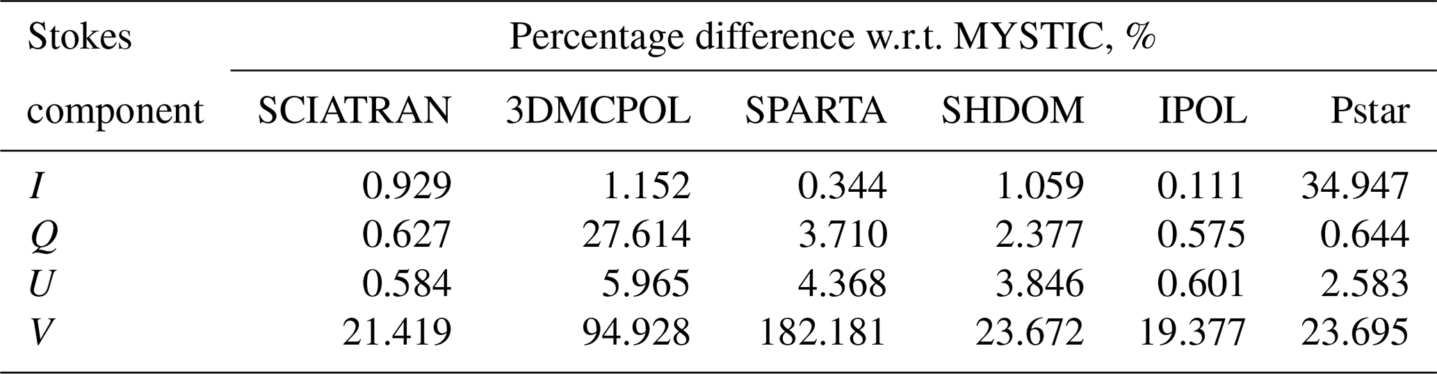
For the decoupled atmospheric radiative transfer mode, a comparison of Stockes vector components at the top and the bottom of the atmosphere for different viewing directions and solar zenith angles with results from MYSTIC (Emde et al., 2010), 3DMCPOL (Cornet et al., 2010), SPARTA (Barlakas et al., 2014), SHDOM (Evans, 1998), IPOL (Korkin and Lyapustin, 2019), and Pstar (Ota et al., 2010) models was performed using rather sophisticated atmospheric scenarios involving a cloud embedded in the atmosphere above the ocean surface. We used the test scenarios and modelling results from the comparison performed by Emde et al. (2015) without participation of SCIATRAN. Details about the RT models intercomparison, test scenarios, and obtained results can be found in the above referenced publication. Here, we summarize the comparison results by providing the percentage differences between different RTMs including SCIATRAN and MYSTIC model calculated as the root-mean-square errors over all observational and illumination geometries and over both locations (top and bottom) in the atmosphere. Results for the multi-layer intercomparison case are presented in Table 1.

Table 1 Percentage differences for the Stokes vector components modelled by SCIATRAN, 3DMCPOL, SPARTA, SHDOM, IPOL, and Pstar with respect to the results from the MYSTIC model (calculated as the root-mean-square errors over all observational and illumination geometries and over both locations (top and bottom) in the atmosphere).

For a coupled atmosphere-ocean system, the downwelling radiation just below the ocean surface (0.001 m depth) calculated with the scalar SCIATRAN RTM was qualitatively compared with the results from a vector 3D Monte Carlo code (You et al., 2009) and vector and scalar versions of the RAY radiative transfer model (Zege and Chaikovskaya, 1996). The results of this comparison were presented by Rozanov et al. (2014). For a flat water interface all three models were found to be in a good agreement. For a wind-roughed ocean surface only comparisons with the Monte Carlo code could be done revealing a good agreement for smaller viewing angles (<50°). For larger viewing angles a larger disagreement is observed because of the small radiance and larger numerical noise of the Monte Carlo model.

These comparisons revealed the impact of polarization on the accuracy of underwater radiation field calculations.

In an earlier publication by Hollstein and Fischer (2012), the impact of polarization was also identified for the top of atmosphere radiance. These results motivated us to implement the treatment of the polarization into the coupled atmosphere-ocean mode of the SCIATRAN model.

To assess the accuracy of SCIATRAN radiative transfer calculations for the coupled atmosphere-ocean system (AOS) accounting for the polarization, the testbed results published by Chowdhary et al. (2020) were used. The latter study provides accurate (at least 10⁻⁵) tabulated results for the reflectance of total and linearly polarized upwelling radiance just above the ocean surface and at the top of atmosphere obtained with scalar and vector RT calculations. These test results were generated using the extended General Adding Program (eGAP) radiative transfer code, based on the doubling/adding method (de Haan et al., 1987) and extended by Chowdhary et al. (2006) to include polarized light scattering in ocean systems.

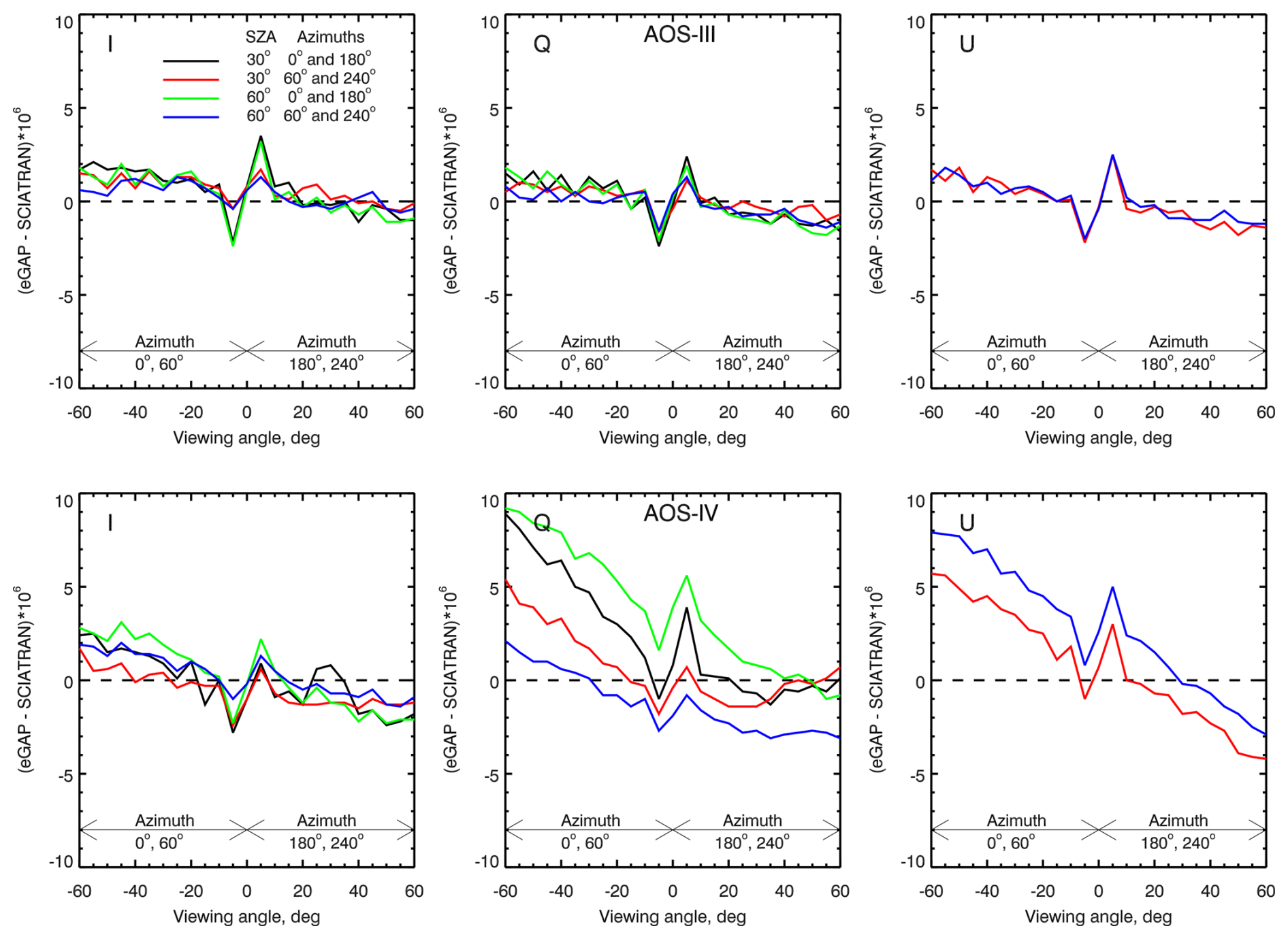
Figure 3 Comparison between the Stokes vector components just above the ocean surface from eGAP and SCIATRAN RT models at a wavelength of 550 nm. The relative differences between the model results are shown as functions of the viewing angle for different solar zenith and azimuth angles for AOS-III (top row) and AOS-IV (bottom row) testbed scenarios (see text). For azimuth angles of 0 and 60° the viewing angles are represented by negative values. The eGAP values used in the comparisons are reported in Table S4 of (Chowdhary et al., 2020) (online version at https://doi.org/10.1016/j.jqsrt.2019.106717).

Here, comparisons for two selected cases are presented: a fully-coupled simple atmosphere-ocean system (AOS-III model according to Chowdhary et al., 2020) containing a molecular atmosphere, rough ocean surface, and pure water and a fully-coupled complex atmosphere-ocean system (AOS-IV model) that includes hydrosols in addition to AOS-III scenario. Comparison results for Stokes vector components just above the ocean surface are presented in Fig. 3 for different solar zenith and viewing angles. It is seen from the plots that SCIATRAN demonstrates very good computational accuracy. In particular, the differences are less than $\mathrm{5}\times {\mathrm{10}}^{-\mathrm{6}}$ for the first Stokes vector component and less than $\mathrm{1}\times {\mathrm{10}}^{-\mathrm{5}}$ for Q and U components. Similar results (not shown here) have been obtained for the radiance at the top of the atmosphere and for other wavelengths.

5  Comparsions with measurement results

Although comparisons with other radiative transfer models and testbed results verify the implementation of various radiative transfer modules, they are usually performed employing significant simplifications. Therefore, only comparison with measurement results can confirm that all physical processes are properly accounted for. This section presents validation results obtained using measurements of spectral albedo and Hemispherical-Directional Reflectance Factor (HDRF) performed for SIM surfaces during different campaigns. The SCIATRAN simulations presented in this section were performed using the same model version as in Sect. 4.

5.1 Measurement data

In order to evaluate the coupled and decoupled modes of the SCIATRAN RTM, selected comparisons between SCIATRAN simulations and measurements of spectral albedo and surface HDRF provided by Malinka et al. (2016, 2018) and Goyens et al. (2018) were performed.

Malinka et al. (2016, 2018) reported spectral sea ice albedo measured during the Polarstern cruise ARK-XXVII/3 from 2 August to 8 October 2012 under different atmospheric conditions (clear or cloudy sky) and for different ice types. The measurements of spectral fluxes were performed with portable spectroradiometer ASD FieldSpecPro III at about 1 m above the surface in the spectral range 350–2500 nm with the spectral resolution of 1 nm. The albedo of the surface was obtained by calculating the ratio of upwelling to downwelling irradiances from these measurements.

Goyens et al. (2018) reported snow HDRF observed by multispectral circular fish-eye radiance camera CE600. The instrument performed simultaneous measurements in 16 020 directions (the angle steps for viewing zenith and azimuth angles were 1 and 2°, respectively) at six wavelengths (406, 438, 494, 510, 560 and 628 nm). The measurements were performed from 25 May to 7 June 2015 in southern Baffin Bay, Nunavut, on the landfast first-year ice for different surface types (e.g. bare ice, snow covered ice, ponded ice).

5.2 Simulations and fitting

The spectral albedo and directional reflection were simulated using the decoupled and coupled SCIATRAN RT models. For the decoupled model, the solution of RTE in the atmosphere was performed using relevant BRDF model as lower boundary condition. For the coupled model, an iterative approach as discussed in Appendix A was employed.

By solving the RTE, intensity of the radiation field (radiance) in the atmosphere is obtained, from which other radiometric variables can be calculated. The directional reflectance is defined as the ratio of the reflected radiance to the flux of the radiation incident to the surface. The spectral albedo is given by the ratio of the upward to the downward radiation flux near the surface. As the modelled intensities and, thus, other derived variables depend on medium characteristics assumed in the radiative transfer modelling (modelling parameters), the latter need to be estimated based on the measured data before performing comparisons of modelled and measured data. This is done by solving the following minimization problem:

$$\begin{array}{}\text{(14)}& \begin{array}{rl}& {∥L_{\mathrm{mes}}(\mathit{\lambda },\mathrm{\Omega })-L(\mathit{\lambda },\mathrm{\Omega },\mathit{x},\mathit{p})-\sum _{i=\mathrm{1}}^N{\displaystyle \frac{\partial L(\mathit{\lambda },\mathrm{\Omega },\mathit{x},\mathit{p})}{\partial x_i}}\mathrm{\Delta }{x}_i∥}^{\mathrm{2}}\\ & ⟶min,\end{array}\end{array}$$

where L_mes and L are the measured and simulated radiometric variables, λ and Ω denote dependence on the wavelength and observation geometry, respectively, vector x consists of modelling parameters which are to be retrieved by solving the minimization problem, vector p contains modelling parameters fixed in accordance with a priori information, and $\partial L/\partial x_i$ is the partial derivative of the radiometric variable with respect to the modelling parameter x_i. The modelling parameters to be retrieved, x_i, depend on the particular comparison scenario and will be discussed below.

All SCIATRAN RTM calculations were performed accounting for the scattering by air (i.e., Rayleigh scattering), scattering and absorption by aerosols as well as absorption by atmospheric gases (O₃, NO₂, O₂, CO₂, and H₂O). In addition, scattering by clouds was accounted for in some comparison scenarios.

5.3 Spectral albedo

The validation of coupled and decoupled SCIATRAN models is performed by comparing the SCIATRAN simulations with the spectral albedo measurements of bright white ice, snow-covered ice and melt ponds on sea ice as previously used by Malinka et al. (2016, 2018).

5.3.1 White ice and snow-covered ice: spectral albedo

In this section, we compare the spectral albedo modelled by SCIATRAN with the results from measurements over the bright white ice, which is an ice layer covered by a layer of aged show, and bright white ice covered by fresh fine-grained snow (Malinka et al., 2016). Below, the latter scenario will be referred to as the snow-covered ice. The measurements were performed on 11 August and 5 September 2012 (Polarstern stations PS80/224 and PS80/323).

In the case of the decoupled model, the lower boundary condition of RTE, see Eq. (A8) in Appendix A, was set in accordance with the analytical reflectance model suggested by Malinka et al. (2016). The modelling parameters to be determined from Eq. (14) are the optical thickness of the snow layer, τ_snow, effective radius of ice crystals, r_eff, and absorption coefficient of the yellow substance, σ_y(λ₀), see Eq. (7). Although effective IOP are meant here, they refer mostly to the upper layer of the fresh fine-grained snow for the snow-covered ice and to the aged snow otherwise. This is because the IOP of a snow layer are mostly determined by its upper few centimetres. In the case of the coupled model, the geometrical thickness of the ice layer, Δz_ice, needs to be determined in addition while the sensitivity of the spectral albedo to the extinction coefficients of the air bubbles and brine inclusions within the interior ice was found to be negligible for τ_snow about 10 and above.

Two runs were done with the coupled RT model employing different approaches to calculate the IOP of the snow layer, one using the stochastic model and the other assuming monodisperse droxtal ice crystals. Following Malinka et al. (2016), only measurements in the spectral range of 350–1350 nm were used in the fitting procedure to avoid strong noise contamination especially under low sun conditions. The retrieved modelling parameters for the coupled and decoupled models are presented in Table 2.

Table 2 Retrieved modelling parameters for the coupled and decoupled RT models.

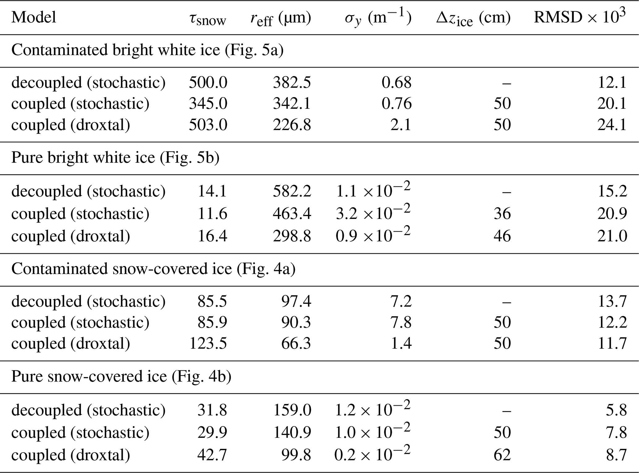
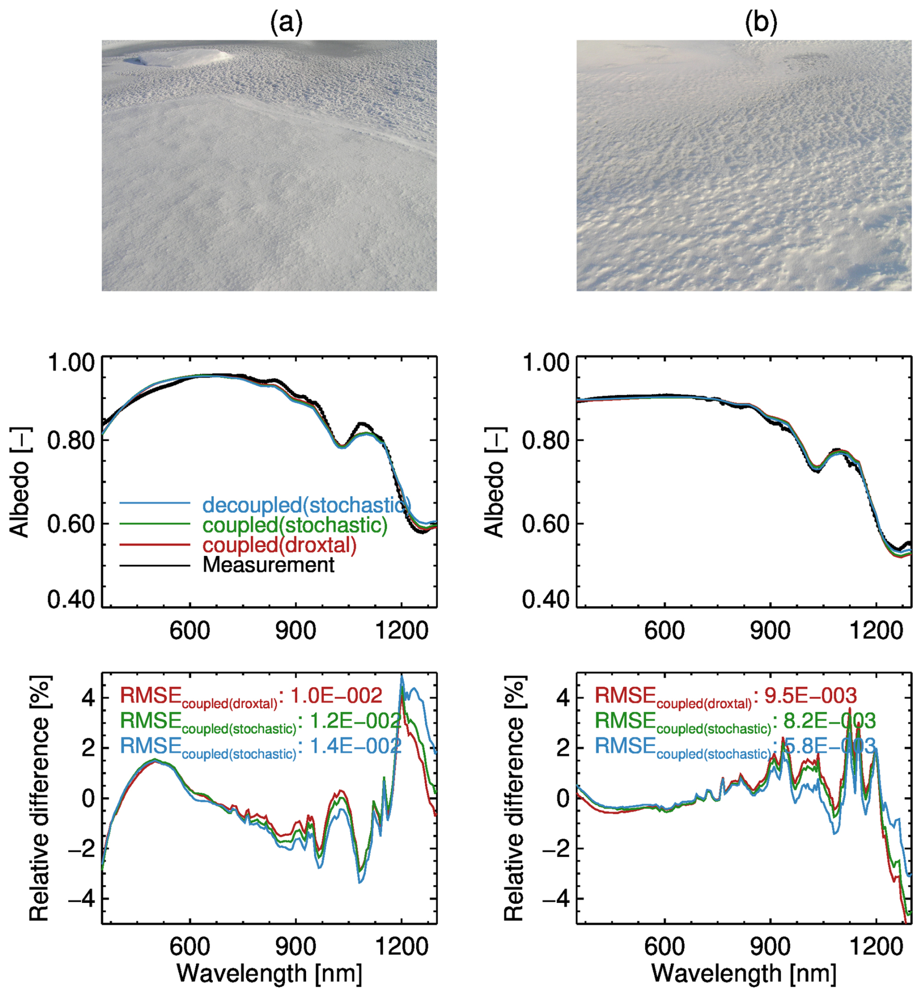
Figure 4 Comparison between the measured and the modelled spectral albedo of snow-covered ice for the examples presented by Malinka et al. (2016) in their Fig. 11a and c. Upper panels: photos of the observation scenes (adopted from Malinka et al., 2016). Middle panels: measured and modelled surface albedo. Lower panels: percentage difference between the measured and modelled spectral albedo.

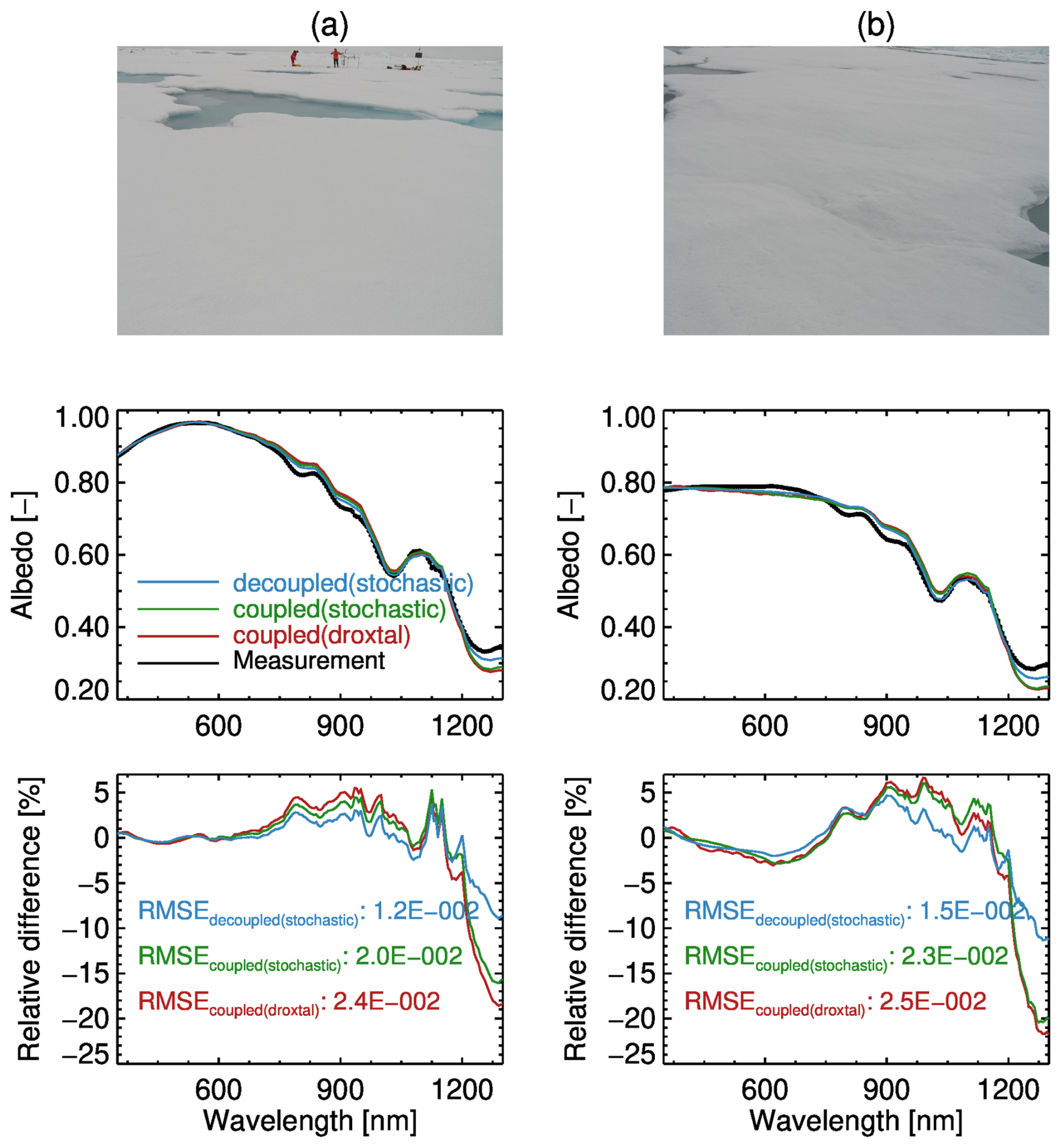
Figure 5 Comparison between the measured and the modelled spectral albedo of bright white ice for the examples presented by Malinka et al. (2016) in their Fig. 8a and c. Upper panels: photos of the observation scenes (adopted from Malinka et al., 2016). Middle panels: measured and modelled surface albedo. Lower panels: percentage difference between the measured and modelled spectral albedo.

Figures 4 and 5 show comparisons of the modelled and measured spectral albedo for the snow-covered and bright white ice, respectively. The left panels in both plots depict scenarios with high contamination by the yellow substance, while the retrieved concentration of the yellow substance for the scenarios shown in the right panels of both plots is negligible. It is seen from the plots that general spectral behaviour of the measured spectral albedo is well reproduced by the model for both scenarios. In particular, one clearly observes a high reflection in the visible spectral range and a low reflection in NIR and SWIR (Short Wave InfraRed). The latter is caused by the ice absorption (Warren, 2019; Mitchell and Arnott, 1994). The local maximum of the spectral albedo at 1.05–1.11 µm is attributed to the local minimum of the imaginary part of the ice refractive index at 1.1 µm (Wiscombe and Warren, 1980; Malinka et al., 2018).

For the snow-covered ice (Fig. 4), the relative differences between the modelled and measured data are mostly within 2 % in the visible spectral range increasing to up to 5 % in NIR and SWIR. These differences are well within the general requirement for the absolute accuracy of the surface albedo (0.02–0.05) in climate models (Pohl et al., 2020a). For the bright white ice (Fig. 5), the model overestimates the absorption of the snow layer in the SWIR spectral range. At wavelengths above 1.2 µm, the difference between the modelled and measured data increases with wavelength to up to −22 %. A possible reason for this discrepancy might be a vertical inhomogeneity of the grain size. A detailed investigation of this topic is, however, beyond the scope of this paper.

In general, the SCIATRAN model represents well the spectral albedo of the snow-covered and bright white ice for both uncontaminated and contaminated by yellow substance snow layers. However, in the SWIR range, larger differences are identified for the bright white ice scenario. Analysing retrieved modelling parameters presented in Table 2, the following findings can be formulated:

• Differences between the retrieved parameters for the coupled and decoupled models are rather small (∼ 20 %). This demonstrates that, for the selected scenarios, the coupling effects play rather a minor role.

• For a snow-covered ice, the retrieved effective radius of ice particles is significantly smaller than that for the bright white ice, which is expected when covering by fine-grained snow. Considering that the absorption by ice crystals increases with their size (Mitchell and Arnott, 1994), one expects smaller albedo in NIR and SWIR ranges for the bight white ice. This is confirmed by Figs. 4 and 5 showing the albedo of ∼ 0.6 for the snow-covered ice and of ∼ 0.4 for the bright white ice at the wavelength of 1.2 µm.

• If the snow layer is assumed to consist of monodisperse droxtal ice crystals, larger optical thicknesses and smaller effective radii are retrieved in comparison to those resulting from the use of the stochastic model.

5.3.2 Melt ponds on sea ice: spectral albedo

In this section, we compare the spectral albedo modelled by SCIATRAN with the results from measurements over melt ponds on sea ice for clear sky and cloudy scenes (Malinka et al., 2018). The measurements were performed in the central Arctic on 10 and 26 August 2012. As stated by Malinka et al. (2018), the selected measurements represent typical types of melt ponds.

In the case of the decoupled model, the lower boundary condition of RTE, see Eq. (A8), was set in accordance with the analytical reflectance model of melt ponds on sea ice suggested by Malinka et al. (2018). The modelling parameters to be determined from Eq. (14) are the ice thickness, water depth, and transport scattering coefficient of the ice layer.

For the coupled model, the spectral albedo was calculated for both Open melt Pond (OP) and Frozen melt Pond (FP) scenarios. In the OP case, the lower medium includes a water layer on the top of sea ice. In the FP scenario, a very thin ice layer (ice crust) is added on the top of the OP lower medium. For both scenarios, the modelling parameters to be determined from Eq. (14) are the top and bottom depths of the sea ice layer and scattering coefficient of the brine inclusions. For the FP scenario, the geometrical thickness of the ice crust is set to a fixed value of 1.5 cm. The scattering within the ice crust layer is assumed to be only due to air bubbles with the scattering coefficient of 80 m⁻¹, which corresponds to an optical thickness of 1.2. The retrieved modelling parameters obtained for the coupled and decoupled RT models are presented in Table 3.

Table 3 Retrieved modelling parameters for the coupled and decoupled RT models.

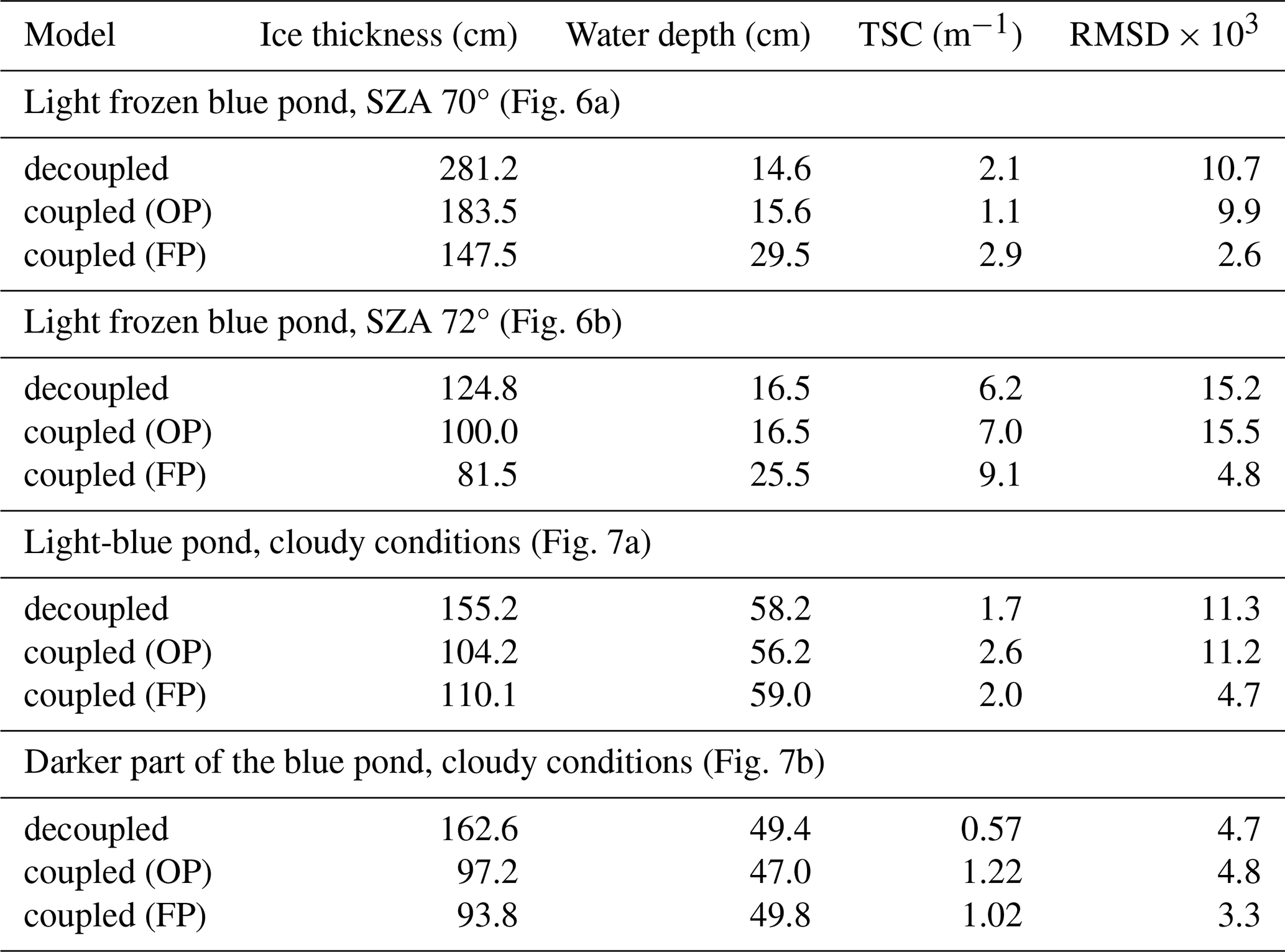
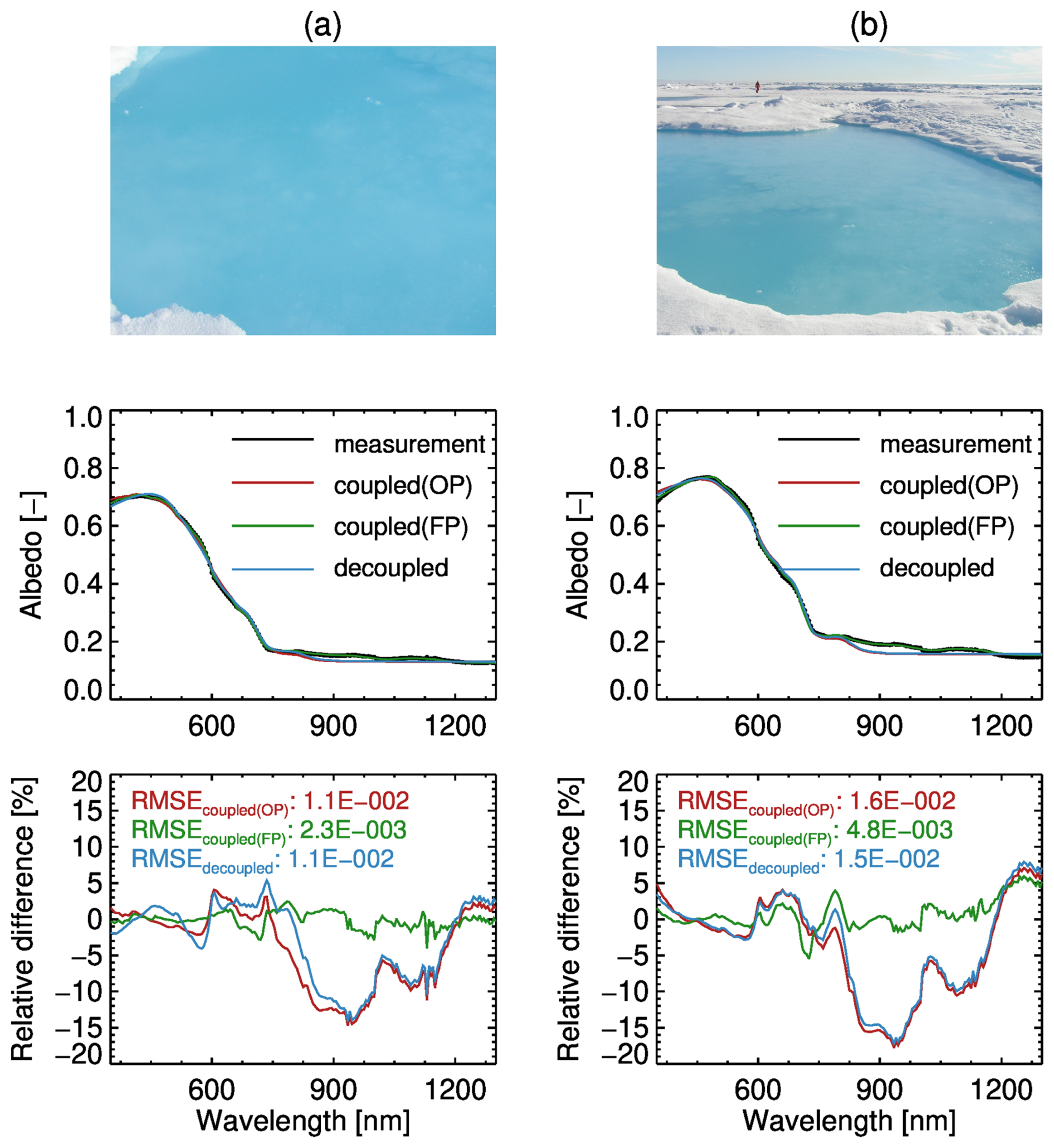
Figure 6 Comparison between the measured and the modelled spectral albedo of the frozen melt ponds for clear sky conditions in accordance with the examples presented by Malinka et al. (2018) in their Fig. 6a and b. Panels (a) and (b) present the results for solar zenith angles of 70 and 72°, respectively. Upper panels: photos of the observation scenes (adopted from Malinka et al., 2018). Middle panels: measured and modelled spectral albedo. Lower panels: percentage difference between the measured and modelled spectral albedo.

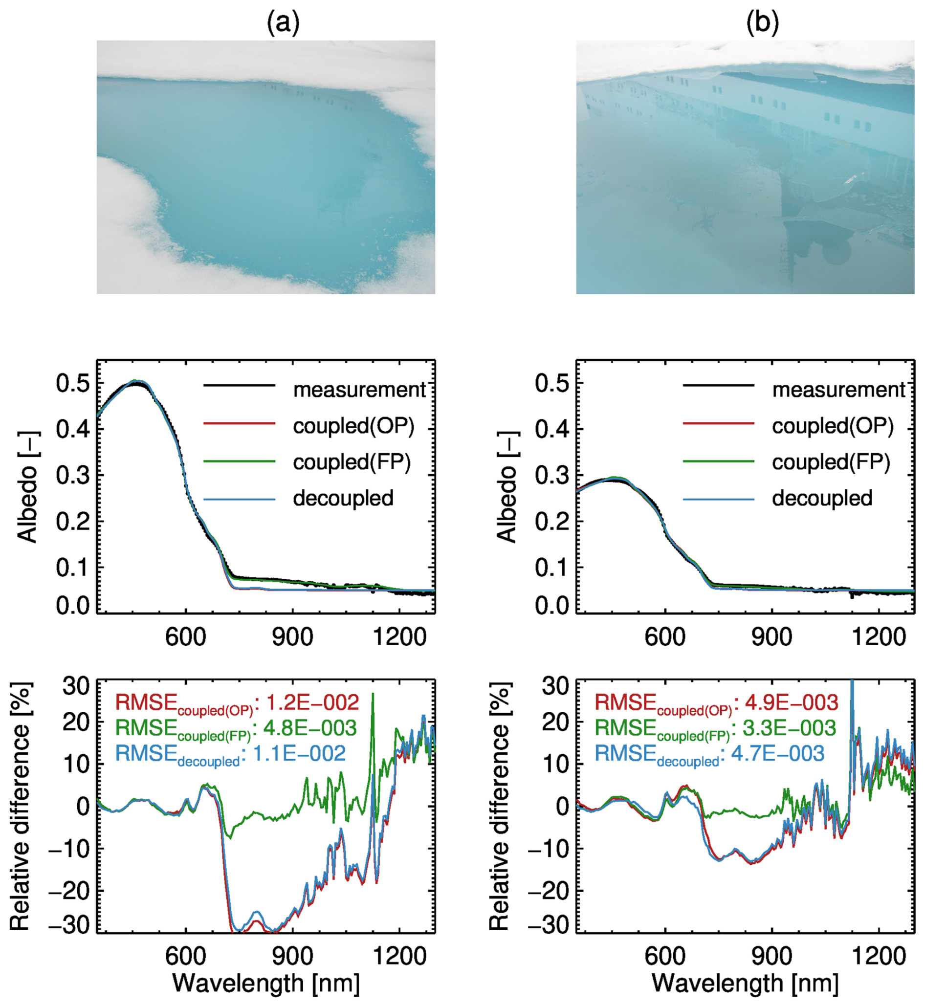
Figure 7 Comparison between the measured and the modelled spectral albedo of the frozen melt ponds for cloudy conditions in accordance with the examples presented by Malinka et al. (2018) in their Fig. 9a and b. Upper panels: photos of the observation scenes (adopted from Malinka et al., 2018). Middle panels: measured and modelled spectral albedo. Lower panels: percentage difference between the measured and modelled spectral albedo.

Figures 6 and 7 show comparisons of the modelled and measured spectral albedo of frozen melt ponds for the clear sky and cloudy conditions, respectively. Although melt ponds generally exhibit a lower albedo in the visible spectral range as compared to bright white ice, it still can reach values of about 0.7 for wavelengths between 400–500 nm for clear sky conditions, see Fig. 6. This might be due to the reflection of the solar light back to the atmosphere by the thick ice layer located below the meltwater (Malinka et al., 2018). For cloudy scenes, the melt ponds albedo shows similar spectral behaviour as for clear sky conditions but has significantly lower values in the visible spectral range.

A distinguishing feature of the melt pond reflection is a strong decrease of the spectral albedo in the NIR range. Unlike the reflection by the bright white ice, there is no local maximum around 1.1 µm and the dependence of the spectral albedo on the wavelength in the NIR spectral range is quite flat. This is because the wavelength dependence of the melt pond reflection in this spectral region is determined by the Fresnel reflection rather than by the absorption of ice crystals.

As it is seen from Figs. 6 and 7, the spectral albedo of the melt ponds modelled by SCIATRAN agrees well with the measured data for both clear sky and cloudy conditions. For both the coupled model using OP scenario and the decoupled model, the modelling accuracy is similar resulting in similar RMSE, as shown in the lower panels of the plots. Both approaches, however, result in an underestimation of the spectral albedo in the NIR range. For these two model runs, the maximum relative difference between the modelled and measured spectral albedo is 15 %–20 % for the clear sky and 10 %–30 % for conditions.

The use of the coupled model with FP scenario significantly improves the modelling accuracy in the NIR spectral range reducing the disagreement between the modelled and measured data to below 5 % for clear sky and below 10 % for cloudy conditions. In the latter case somewhat larger differences are still seen in the SWIR spectral range. The observed difference between the modelling results when using FP and OP scenarios can be explained by the fact that the absorption of the light occurs within the ice crust layer in the former case and in the water in the latter case. A distinct difference in the imaginary parts of the refractive indices of ice and water in this spectral range (not shown here) confirms this explanation.

5.4 Directional reflectance

To validate the directional distribution of the reflected radiance in the framework of the coupled SCIATRAN model, we compared the HDRF modelled by SCIATRAN with measurement results for melting snow, bare ice, and melt ponds on sea ice reported by Goyens et al. (2018).

Using the intensity of the radiation field modelled by SCIATRAN, HDRF is calculated as follows:

$$\begin{array}{}\text{(15)}& L(\mathit{\lambda },\mathrm{\Omega })=\mathit{\pi }{\displaystyle \frac{I(\mathit{\lambda },\mathrm{\Omega })}{E\left(\mathit{\lambda }\right)}},\end{array}$$

where I(λ,Ω) is the radiance upwelling from a surface illuminated by diffuse and direct solar radiation and E(λ) is the downward total flux. Following Goyens et al. (2018), wavelengths of 438, 560 and 628 nm were selected for this study and radiometric variables I(λ,Ω) and E(λ) were calculated at the altitude of 2 m above the surface corresponding to the position of the CE600 radiance camera. Radiative transfer calculations were performed using the following settings:

• Snow and ice: Geometrical thicknesses of snow and ice layers as well as depth of melt ponds were selected according to data presented by Goyens et al. (2018). Other required micro-physical and optical parameters were determined by fits or set in accordance with a priori information (see below for details).

• Atmosphere: A weakly absorbing aerosol type (Mei et al., 2020b) with AOT of 0.04 at 550 nm was selected, which represents typical background conditions in the Arctic (Mei et al., 2020a, b). Other atmospheric parameters such as pressure, temperature, and gaseous absorber concentrations were taken from the monthly zonal mean dataset generated by the Bremen 2D chemical transport model (Sinnhuber et al., 2009) for May at 65° N.

5.4.1 HDRF of melting snow

In this section, the HDRF modelled by SCIATRAN is compared to multi-directional measurements of the upwelling radiation conducted on 25 May 2015 at the GreenEdge ice camp at the beginning of the snow melting (Goyens et al., 2018). The measurements were performed at a solar zenith angle of 63.56° and the sky conditions were reported as variable.

In accordance with (Goyens et al., 2018), the geometrical thicknesses of the snow layer and of the underlying ice layer were about 30 and 130 cm, respectively. Employing the stochastic model of snow (see Sect. 3.1.1) to calculate the IOP, the optical thickness of the snow layer was estimated to be about 300. This was done by calculating the snow layer extinction coefficient using Eq. (6) with the volume fraction of ice, N_c, set to 0.3 and the mean chord length of ice crystals, a, set to 0.3 mm. The latter value was selected in accordance with a typical snow grain radius of beginning melting snow of about 0.4 mm reported by Goyens et al. (2018) and references therein. The volume fraction of ice was calculated from Eq. (1) using the ice density of 0.917 g cm⁻³ and the snow density of 0.28 g cm⁻³. The latter was selected in accordance with observations during the SnowEx17 campaign (Mei et al., 2021b).

A sensitivity study performed using the coupled SCIATRAN model showed that, for an optical thickness of the snow layer of about 300, the HDRF depends only weakly on the optical parameters of the underlying ice layer, on the variation of snow optical thickness, and on the effective radius of ice crystals. Therefore, no fit of the modelled HDRF with respect to measured data was performed.

As clouds in the atmosphere can change the angular distribution of the downwelling diffuse radiation and cloudiness situation during the measurements was not precisely described by Goyens et al. (2018), the comparison between the modelled and the measured HDRF was done for several model runs: one for clear sky conditions and three for cloudy scenes with different cloud optical thicknesses (COT).

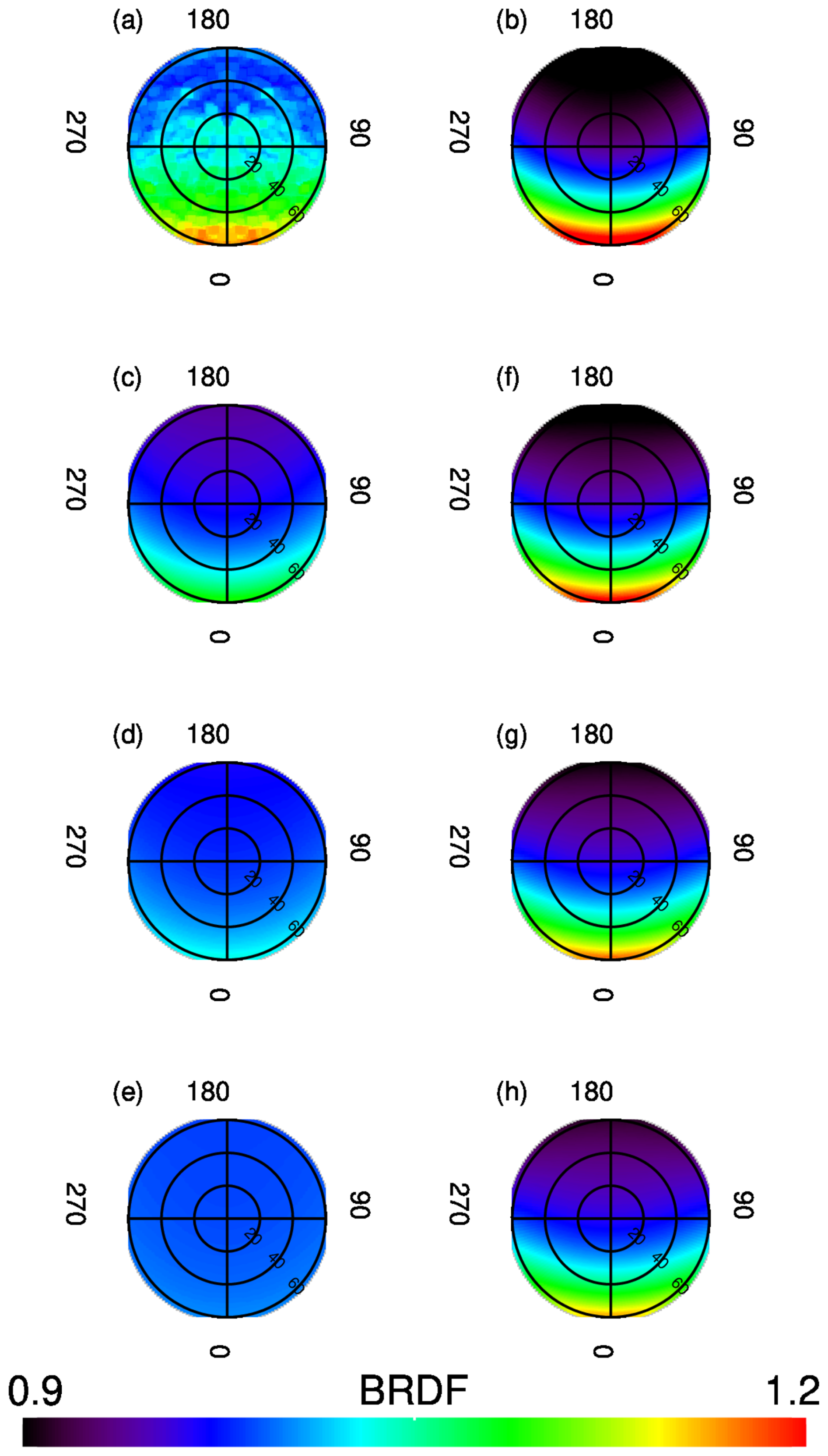
Figure 8 Measured HDRF of melting snow (a) and HDRF modelled under different cloudiness conditions (b–h). (b) Clear sky conditions. (c–e) Diffuse and direct radiation are modelled for cloudy skies with COT 2, 4, and 8, respectively. (f–h) Same as (c)–(e) but with the direct radiation calculated under clear sky conditions.

The impact of clouds on the angular distribution of the reflected radiance modelled with SCIATRAN is illustrated in panels (b)–(e) of Fig. 8. It is evident that in the backward directions (azimuth angle $\mathit{\phi }\in [\mathrm{90},\mathrm{270}\mathit{°}]$), the HDRF for cloudy scenes is higher compared to that for clear sky conditions and shows better agreement with the measurements. However, in the forward directions (azimuth angles $\mathit{\phi }\in [\mathrm{0},\mathrm{90}\mathit{°}]$ and $\mathit{\phi }\in (\mathrm{270},\mathrm{360}\mathit{°}$)), the situation drastically changes as glint conditions are approached. Here, the HDRF for the clear sky is significantly higher than that for cloudy scenes and exceeds the measured HDRF. This behaviour is explained by the fact that the radiation reflected around the glint direction originates mostly from the reflection of the direct solar light while for off-glint directions contribution from the downwelling diffuse radiation is essential. Thus, the observed differences in the agreement between the modelled and measured data for different directions and cloud scenarions might be caused by the horizonthal inhomogeneities in the cloud coverage.

In the framework of a 1D RT model, the presence of a cloud results in a strong attenuation of the direct solar radiation. This attenuation might, however, be inappropriate to desribe observations under inhomogeneous cloud coverage conditions. To demonstrate the impact of the attenuation of the direct solar radiation by a cloud, we calculated the HDRF combining the diffuse downwelling radiation modelled for cloudy conditions and direct solar radiation calculated for clear sky conditions. The results obtained for cloudy scenes with COT of 2, 4, and 8 are presented in Fig. 8f–h, respectively. It is apparent that the usage of the direct solar radiation not affected by clouds significantly improves the agreement with the measurements in the forward direction region. However, the model still underestimates the HDRF for the backward directions.

For the results presented in panels (f)–(h) of Fig. 8, the minimum RMSE occurs for COT = 8, where the RMSE is about 36 % lower compared to that for clear sky conditions and 22 % smaller compared to that for the cloudy scenario with COT = 2. For this reason we chose COT = 8 to illustrate the agreement of the measured and modelled HDRF at different wavelengths, see Fig. 9. Contrary to the measured data, the modeled HDRF does not exhibit any irregular patterns at any wavelength. The irregular patterns seen in the relative differences between the modeled and measured HDRF coincide with those in the measured data. This is a clear indication of an atmospheric inhomogeneity (such as inhomogeneous cloud coverage) or variations in the surface reflection properties, which currently cannot be considered in the fremework of the SCIATRAN RTM. In the glint range, the difference between the modelled and measured data reaches about 5 % for all wavelengths.

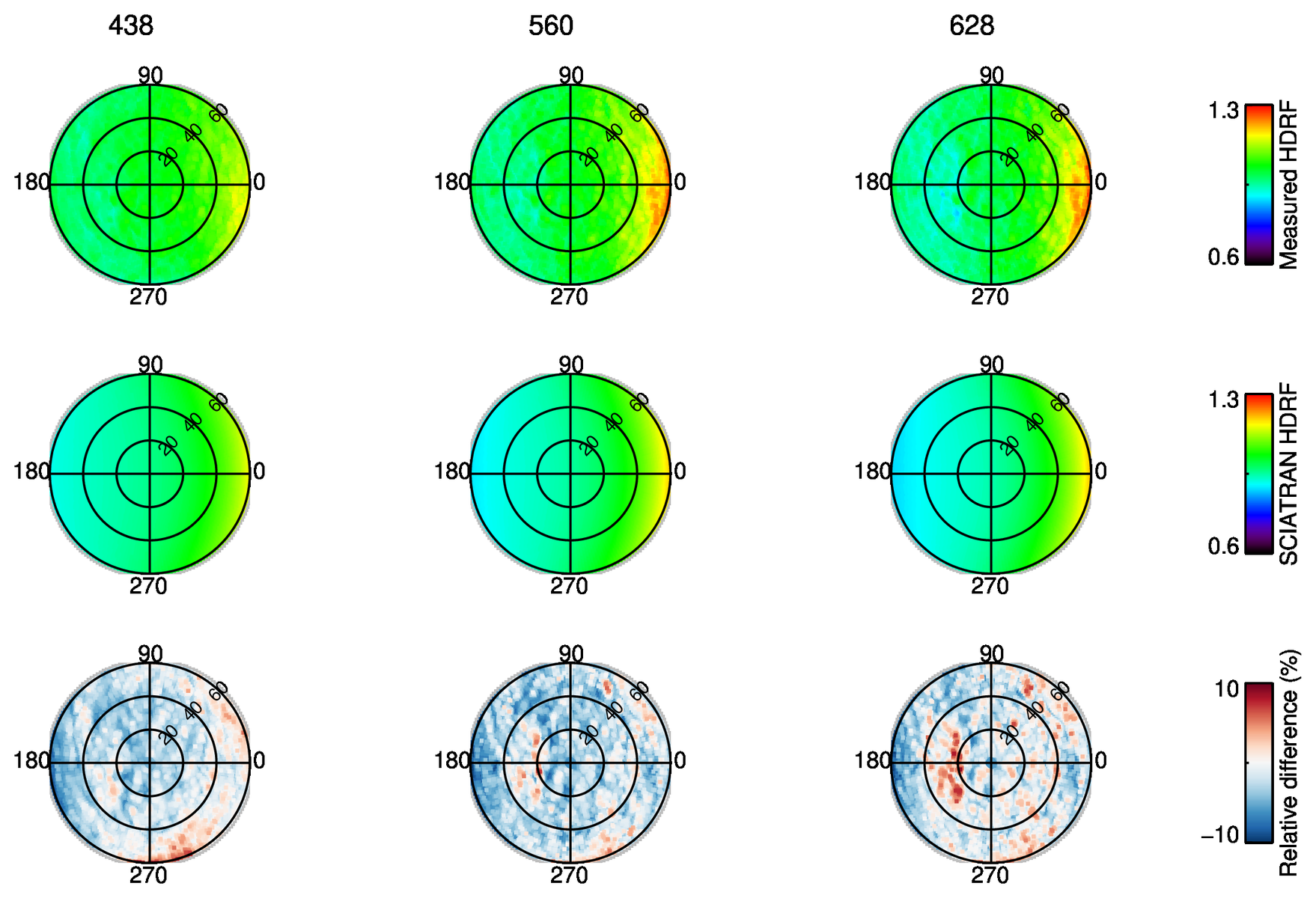
Figure 9 Comparison of the measured and modelled HDRF of melting snow at three wavelengths: 438, 560 and 628 nm (from left to right). Upper panels: measured HDRF. Middle panels: HDRF simulated with the coupled SCIATRAN model calculating the direct solar radiation under clear sky conditions and the diffuse radiation under cloudy conditions with COT = 8. Lower panels: percentage difference between the measured and modelled HDRF.

A similar comparison was performed for the decoupled SCIATRAN model. In this case, the BRDF model developed by Malinka et al. (2016) was used to represent the snow reflectance. All other settings remained unchanged. The comparison with the measured HDRF for the decoupled model (not shown here) reveals similar RMSE as for the coupled model. Similar comparison results for the coupled and decoupled models in the considered case are expected because the main assumptions of the latter, such as weak absorption and large but finite optical thickness, are valid.

5.4.2 HDRF of bare ice

In this section, the HDRF modelled by SCIATRAN is compared to multi-directional measurements of the upwelling radiation conducted on 1 June 2015 over bare ice (Fig. 6d–f in Goyens et al., 2018). The sea ice surface was manually cleaned from the snow cover and described by Goyens et al. (2018) as a flat grey-bluish ice surface with a thin surface scattering layer (< 2 cm) consisting of coarse ice grains. The measurements were performed at a solar zenith angle of 59.52° at clear sky conditions.

In the SCIATRAN model, a bare ice surface with a scattering layer on its top and a flat interface between the scattering layer and the interior ice was assumed. This parameterization follows Grenfell and Perovich (2004), who suggested to represent the structure of sea ice by up to three distinct layers. Specifically, they state that “when the melt season began, most of the brine drained out of the upper layers of the ice, producing a `surface scattering layer' that persisted throughout the melt season”. A photo of a representative ice core with a drained surface layer is shown in Fig. 4 of Grenfell and Perovich (2004).

In accordance with Goyens et al. (2018), the geometrical thickness of the scattering layer was set to 2 cm and that of the ice layer to 130 cm. The IOP of the scattering layer were calculated assuming the stochastic model (see Sect. 3.1.1). The IOP of the interior ice were modeled assuming scattering by brine inclusions, air bubbles, and absorption of pure ice.

The selected HDRF model of the bare ice requires the input of two parameters of the scattering layer (effective radius of ice grains and optical thickness) and of two parameters of the interior ice (scattering coefficient of air bubbles, σ_a, and of brine inclusions, σ_b). To reduce the number of parameters to be retrieved, we followed Grenfell and Perovich (2004) and set the effective radius of ice grains in the scattering layer to a fixed value of 1.5 mm. This approach is reasonable beacase of a weak absorption of ice in the considered spectral range resulting in a weak sensitivity of the directional reflectance to the assumed grain size.

Although the HDRF was measured at 10 260 directions, simultaneous estimation of both σ_a, and σ_b was impossible because of a strong correlation between their weighting functions. Therefore, the fitting was performed assuming that the scattering in the ice layer is caused by either air bubbles or by brine inclusions. This means that the retrieval process was performed twice for each wavelength. First, setting σ_b=0, we retrieved σ_a and the optical thickness of the scattering layer, τ. Thereafter, setting σ_a=0, we retrieved σ_b and τ. In the following discussion, two values separated by a slash denote fitting results obtained assuming the scattering by either air bubbles or by brine inclusions. The calculation of the HDRF was performed assuming wavelength-independent asymmetry parameters of the Henyey–Greenstein phase function of 0.86 for air bubbles and 0.99 for brine inclusions.

Initial retrievals showed that ${\mathit{\sigma }}_{\mathrm{a}}/{\mathit{\sigma }}_{\mathrm{b}}$ at 438 nm were almost twice as small as those at 628 nm.

This contradicts the fact that the scattering coefficient of a particle which is much larger than the wavelength must be independent of the wavelength. This discrepancy can be explained by a presence of an additional absorber in the interior ice whose absorption coefficient is maximal at 438 nm and minimal at 628 nm. As there was no information about absorbing species in the ice layer from in situ measurements performed during the measurement campaign, the yellow substance (see Sect. 3.1.2) was assumed to be a possible contaminant. To estimate the absorption coefficient of the yellow substance, the fitting process was repeated independently for wavelengths 438, 560, and 628 nm setting σ_y(λ₀) to $\mathrm{0},\mathrm{0.1},\mathrm{0.2},\mathrm{0.3},\mathrm{0.4},$ and 0.5 m⁻¹. We remind that λ₀=390 nm. It was found that σ_y(λ₀)=0.2 m⁻¹ provides minimum difference between the retrieved scattering coefficients of ice at 438 and 628 nm. Therefore, this value was considered a reasonable estimation of the yellow substance absorption coefficient.

Table 4 Fitting results for the bare ice contaminated by the yellow substance with the absorption coefficient of 0.2 m⁻¹ at 390 nm. Results obtained for the scattering either by air bubbles or by brine inclusions are separated by a slash.

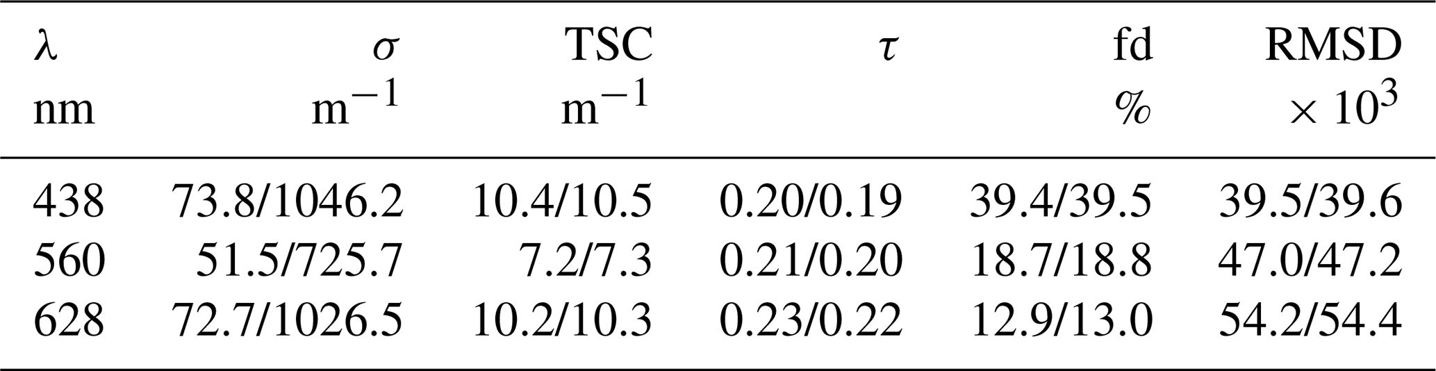
An overview of the retrieved parameters is presented in Table 4. The optical thickness of the scattering layer is estimated to be 0.19–0.23 depending on the wavelength. Note that this refers to the optical thickness of the scattering layer, not the geometric thickness of the ice. The transport scattering coefficient of the bare ice is estimated to be 7.2–10.5 m⁻¹. The value at 560 nm is significantly smaller (∼30 %) than those at 438 and 628 nm. This suggests that either the absorption by yellow substance, as described by Eq. (7), is too weak at the wavelength of 560 nm or other absorbers are present.

Figure 10 displays a comparison of the measured and simulated HDRF for the bare ice. The top row of the plot shows the measured HDRF at three different wavelengths: 438, 560 and 628 nm. The observed irregularity of the HDRF angular distribution indicates a presence of horizontal surface inhomogeneities. As suggested by Goyens et al. (2018), these inhomogeneities might be attributed to remaining snowpacks on the ice surface.

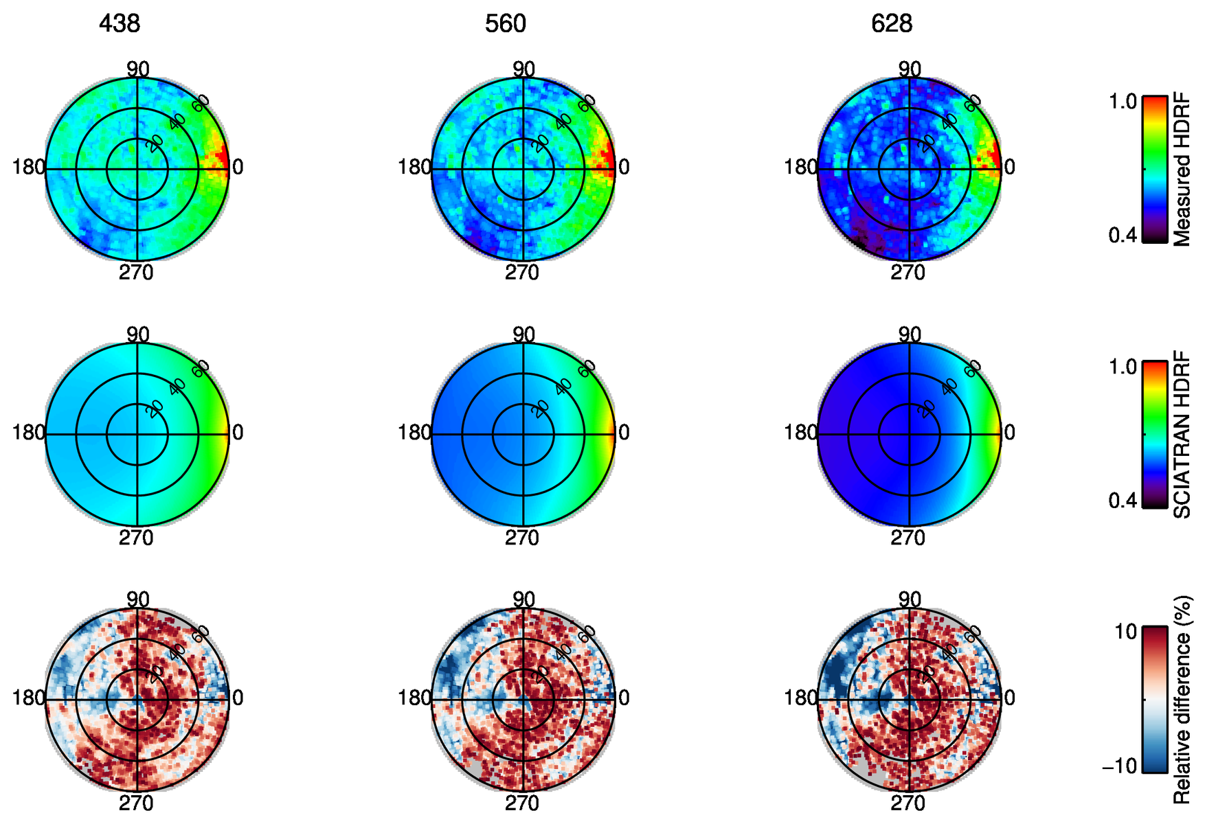
Figure 10 Comparison of the measured and modelled HDRF of bare ice at three wavelengths: 438, 560 and 628 nm (from left to right). Upper panels: measured HDRF. Middle panels: HDRF simulated with the SCIATRAN model. Lower panels: percentage difference between the measured and modelled HDRF. The calculations were done for the example presented by Goyens et al. (2018) in Fig. 6d–f (CE60060ice).

5.4.3 HDRF of the melt ponds on sea ice

In this section, HDRF for melt ponds on sea ice modelled by SCIATRAN is compared with measurements conducted at the GreenEdge ice camp on 7 June 2015 as reported by Goyens et al. (2018). In the SCIATRAN model, the optical properties of the under-pond ice layer were represented by absorption by pure ice and scattering by brine inclusions and air bubbles. In accordance with Goyens et al. (2018), the pond depth and under-pond ice thickness were set to 11 and 120 cm, respectively.

The model initialisation parameters to be obtained by the fit are the root mean square value of the isotropic Gaussian shape, σ², and ice scattering coefficient (represented by the scattering coefficient of air bubbles, σ_a, or brine inclusions, σ_b). The fitting in the principal plane, where the impact of specular reflection is maximal, results in ${\mathit{\sigma }}^{\mathrm{2}}=\mathrm{1.7}\times {\mathrm{10}}^{-\mathrm{4}}$. Similar to the bare ice, simultaneous estimation of both σ_a and σ_b was impossible because of a strong correlation between their weighting functions. Therefore, the fitting was performed twice assuming that the scattering in the ice layer is caused solely by either air bubbles or by brine inclusions. In the text below, the corresponding fitting results are separated by a slash. An overview of the retrieved parameters is presented in Table 5. The transport scattering coefficient of the interior ice is estimated to be in the range of 1.42–1.62 m⁻¹ which is significantly smaller than for the bare ice.

Table 5 Fitting results for a melt pond with a rough atmosphere-ocean interface. Results obtained for the scattering either by air bubbles or by brine inclusions are separated by a slash.

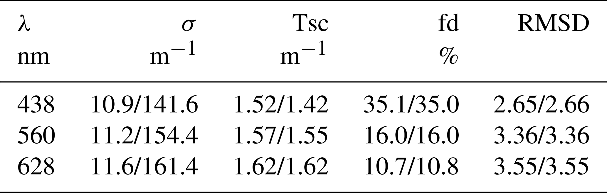
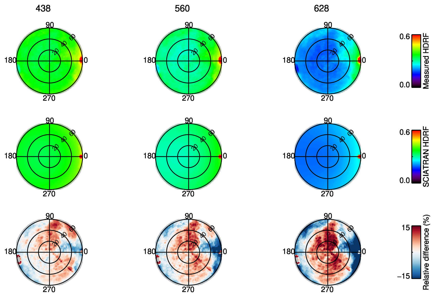
Figure 11 Comparison of the measured and modelled HDRF for a melt pond on sea ice at three wavelengths: 438, 560 and 628 nm (from left to right). Upper panels: measured HDRF. Middle panels: HDRF modeled with the SCIATRAN model. Lower panels: percentage difference between the measured and modelled HDRF. The calculations were done for the example presented by Goyens et al. (2018) in Fig. 6g–i (CE60056meltpond).

Figure 11 shows the measured and modelled HDRF at 438, 560, and 628 nm wavelengths. A strong forward peak caused by the Fresnel reflection on the atmosphere-ocean interface is observed in the measurements and well reproduced by the SCIATRAN model. However, the peak in the measured data is wider, which might be related to a slight roughness of the water surface or a finite angular dimension of the solar disk, which is not accounted for in the SCIATRAN model. Typically, the relative difference between the modelled and measured data is within ± 15 %. Larger relative differences at 628 nm result from a significantly lower reflection at this wavelength as compared to that at 438 and 560 nm. The model calculations were performed assuming a cloud free atmosphere, although rapid variations in sky conditions (alternation of clear sky and diffuse cloud coverage) were reported by Goyens et al. (2018). Contrary to the melting snow scenario discussed in Sect. 5.4.1, no improvement in the agreement between the measured and modelled data was observed when performing modelling runs for a cloudy atmosphere.

6 Conclusion

This paper discusses new developments to extend the capabilities of the radiative transfer model SCIATRAN (Rozanov et al., 2014, 2017, 2021; Mei et al., 2023) for cryospheric science applications, specifically in simulating radiative transfer processes through snow, ice and melt ponds on sea ice. In particular, we focus on the discussion of the implementation details of the inherent optical properties of snow and ice layers.

The newly implemented features are verified by comparisons with other radiative transfer models and with measurement data. In particular, selected comparisons between SCIATRAN modelling results and measurements of the spectral albedo and highly angular-resolved Hemispherical-Directional Reflectance Factor (HDRF) of the snow and ice are presented and show a good agreement between the measured and modelled results.

Unlike existing RTMs developed specifically for modelling the light reflection by snow, ice, and melt ponds, the new SCIATRAN model is an extension of its previous version and features all capabilities which have been previously used for a wide range of applications, such as the scattering by aerosols and clouds, absorption by gases, and reflection by the surface (Mei et al., 2023). The most recent version of SCIATRAN is capable of simulating radiative transfer processes in a vertically inhomogeneous coupled atmosphere-snow(water)-ice-water system. Modelling of the radiation field in the atmosphere can be performed using both coupled and decoupled modes of the SCIATRAN RTM. In the later case, different BRDF models of the surface reflection are available, which is offered by only a few of the existing RTMs.

The most recent version of the SCIATRAN software is freely distributed via the web-page of the Institute of Environmental Physics (IUP), University of Bremen (https://www.iup.uni-bremen.de/sciatran/, last access: 23 June 2026) under GNU LGPL V3.0 license.

Appendix A: Formulation of the boundary value problem for a coupled and decoupled radiative transfer model

Under assumptions formulated by Rozanov et al. (2014) in the beginning of their Sect. 4, the vector radiative transfer equation is written as

$$\begin{array}{}\text{(A1)}& \mathit{\mu }{\displaystyle \frac{\partial }{\partial \mathit{\tau }}}\mathit{I}(\mathit{\tau },\mathrm{\Omega })=-\mathit{I}(\mathit{\tau },\mathrm{\Omega })+\mathit{J}(\mathit{\tau },\mathrm{\Omega })+{\mathit{J}}_{\mathrm{e}}(\mathit{\tau },\mathrm{\Omega }).\end{array}$$

Here, I(τ,Ω) is the Stokes vector whose components, $I,U,Q,V$ are defined according to Mishchenko et al. (2002, 2006), J(τ,Ω) and J_e(τ,Ω) denote the scattering and internal emission source functions, respectively. The thermal emission is not modelled in this study. $\mathit{\tau }\in [\mathrm{0},{\mathit{\tau }}_{\mathrm{0}}]$ is the optical depth changing from τ=0 at the top to τ=τ₀ at the bottom of the medium, and the variable $\mathrm{\Omega }:=\mathit{\{}\mathit{\mu },\mathit{\phi }\mathit{\}}$ represents a pair of angular variables, $\mathit{\mu }\in [-\mathrm{1},\mathrm{1}]$ and $\mathit{\phi }\in [\mathrm{0},\mathrm{2}\mathit{\pi }]$. Here, μ is the cosine of the polar angle ϑ measured from the positive τ-axis (directed opposite to the z-axis) and φ is the azimuthal angle measured from the positive x-axis in the clockwise direction when looking in the direction of the positive z-axis (see Fig. 1 in Rozanov et al., 2014). The scattering source function is given by

$$\begin{array}{}\text{(A2)}& \mathit{J}(\mathit{\tau },\mathrm{\Omega })={\displaystyle \frac{\mathit{\omega }\left(\mathit{\tau }\right)}{\mathrm{4}\mathit{\pi }}}\underset{\mathrm{4}\mathit{\pi }}{\int }\mathbf{Z}(\mathit{\tau },\mathrm{\Omega },{\mathrm{\Omega }}^{\prime })\mathit{I}(\mathit{\tau },{\mathrm{\Omega }}^{\prime })\mathrm{d}{\mathrm{\Omega }}^{\prime },\end{array}$$

where ω(τ) is the single scattering albedo (scattering coefficient divided by the extinction coefficient) and $\mathbf{Z}(\mathit{\tau },\mathrm{\Omega },{\mathrm{\Omega }}^{\prime })$ is the phase matrix describing the scattering properties of the medium. In a local thermodynamic equilibrium (assumed here), the internal emission source function J_e(τ,Ω) is represented as

$$\begin{array}{}\text{(A3)}& {\mathit{J}}_{\mathrm{e}}(\mathit{\tau },\mathrm{\Omega })=[\mathrm{1}-\mathit{\omega }(\mathit{\tau }\left)\right]B\left[T\right(\mathit{\tau }\left)\right]{\mathit{l}}_{\mathrm{1}},\end{array}$$

where B[T(τ)] is the Planck function (see e.g. Lenoble, 1993; Liou, 2002 for details), T(τ) is the kinetic temperature of the medium, the vector ${\mathit{l}}_{\mathrm{1}}=[\mathrm{1},\mathrm{0},\mathrm{0},\mathrm{0}{]}^{\mathrm{T}}$ indicates that the thermal emission is unpolarized, and the superscript T denotes the transpose operation.

The phase matrix $\mathbf{Z}(\mathit{\tau },\mathrm{\Omega },{\mathrm{\Omega }}^{\prime })$ is closely related to the scattering matrix F(τ,γ) that describes a transformation of the Stokes vector as a result of scattering by a volume element. The scattering matrix F(τ,γ) relates the Stokes vectors of the incident and scattered waves with the Stokes vectors defined with respect to the scattering plane. The latter is drawn through the propagation directions of the incident and scattered waves. In general, the Stokes vector of the radiation field is defined with respect to the meridional plane, which does not have to coincide with the scattering plane. Therefore, a rotation of the reference plane of both the incident wave before the scattering process and the scattered wave thereafter is needed to apply the scattering matrix. The entire transformation (including two rotations) is described by the phase matrix, $\mathbf{Z}(\mathit{\tau },\mathrm{\Omega },{\mathrm{\Omega }}^{\prime })$, and an analytical relationship between the phase matrix and the scattering matrix is presented among others by Chandrasekhar (1950), Mishchenko et al. (2002), and Hovenier et al. (2004).

To solve VRTE given by Eq. (A1) one needs to define optical properties of a medium and formulate boundary conditions. Usually, the boundary conditions are formulated as follows. At the top of the atmosphere, the incident solar radiation is assumed to be a monodirectional unpolarized light beam with an infinite extension in space. The solar zenith angle, ϑ₀, is defined as the angle between the positive direction of the z-axis and the direction to the Sun. The x-axis of the basic coordinate system is chosen to point away from the Sun. This means that the azimuthal angle of the solar beam is equal to zero (φ₀=0°). The Stokes vector of the direct solar light is written as $F_{\mathrm{0}}\mathit{\delta }(\mathit{\mu }-{\mathit{\mu }}_{\mathrm{0}})\mathit{\delta }(\mathit{\phi }-{\mathit{\phi }}_{\mathrm{0}}){\mathit{l}}_{\mathrm{1}}$, where δ(μ−μ₀) and δ(φ−φ₀) are the Dirac delta functions (Korn and Korn, 1968), μ₀ is the cosine of the solar zenith angle, and F₀ is the solar irradiance (extraterrestrial solar flux). Throughout this study we assume that the explicit notation of the wavelength dependence for all relevant quantities is omitted.

The upper boundary condition is formulated then as

$$\begin{array}{}\text{(A4)}& {\mathit{I}}_{\mathrm{a}}(\mathrm{0},\mathit{\mu },\mathit{\phi })=F_{\mathrm{0}}\mathit{\delta }(\mathit{\mu }-{\mathit{\mu }}_{\mathrm{0}})\mathit{\delta }(\mathit{\phi }-{\mathit{\phi }}_{\mathrm{0}}){\mathit{l}}_{\mathrm{1}}.\end{array}$$

At the lower boundary of the considered plane-parallel medium, we assume a flat or roughed interface. The lower boundary condition is written as follows:

$$\begin{array}{}\text{(A5)}& \begin{array}{rl}& {\mathit{I}}_{\mathrm{a}}({\mathit{\tau }}_{\mathrm{0}},\mathit{\mu },\mathit{\phi })={\mathcal{R}}_{\mathrm{a}}{\mathit{I}}_{\mathrm{a}}({\mathit{\tau }}_{\mathrm{0}},{\mathrm{\Omega }}^{\prime })+{\mathcal{T}}_{\mathrm{oa}}{\mathit{I}}_{\mathrm{o}}(\mathrm{0},{\mathrm{\Omega }}^{\prime }),\\ & \mathit{\mu }<\mathrm{0},\end{array}\end{array}$$

where ${\mathit{I}}_{\mathrm{a}}({\mathit{\tau }}_{\mathrm{0}},{\mathrm{\Omega }}^{\prime })$ and ${\mathit{I}}_{\mathrm{o}}(\mathrm{0},{\mathrm{\Omega }}^{\prime })$ are the Stokes vectors of the radiation field just above and just below the air–water interface, respectively,

$$\begin{array}{rl}& {\mathcal{R}}_{\mathrm{a}}=\underset{\mathrm{0}}{\overset{\mathrm{2}\mathit{\pi }}{\int }}\mathrm{d}{\mathit{\phi }}^{\prime }\underset{\mathrm{0}}{\overset{\mathrm{1}}{\int }}\mathrm{d}{\mathit{\mu }}^{\prime }{\mathit{\mu }}^{\prime }{\mathbf{R}}_{\mathrm{a}}(\mathrm{\Omega },{\mathrm{\Omega }}^{\prime })\otimes \mathrm{and}\\ & {\mathcal{T}}_{\mathrm{oa}}=\underset{\mathrm{0}}{\overset{\mathrm{2}\mathit{\pi }}{\int }}\mathrm{d}{\mathit{\phi }}^{\prime }\underset{-\mathrm{1}}{\overset{\mathrm{0}}{\int }}\mathrm{d}{\mathit{\mu }}^{\prime }{\mathbf{T}}_{\mathrm{oa}}(\mathrm{\Omega },{\mathrm{\Omega }}^{\prime })\otimes \end{array}$$

are the linear integral operators, ${\mathbf{R}}_{\mathrm{a}}(\mathrm{\Omega },{\mathrm{\Omega }}^{\prime })$ and ${\mathbf{T}}_{\mathrm{oa}}(\mathrm{\Omega },{\mathrm{\Omega }}^{\prime })$ are 4 × 4 matrices determining the angular reflection and transmission properties of the ocean-atmosphere interface. We remind that the second term in Eq. (A5) is often referred to as the water-leaving radiation. The subscripts “a” and “o” are used here and below to distinguish between the parameters of the radiation field within the atmosphere and within the ocean, respectively. The symbol ⊗ is used here and below to highlight the fact that one deals with an integral operator rather than a finite integral. Analogously to Eq. (A5), the upper boundary condition for the lower medium is written as

$$\begin{array}{}\text{(A6)}& \begin{array}{rl}& {\mathit{I}}_{\mathrm{o}}(\mathrm{0},\mathit{\mu },\mathit{\phi })={\mathcal{R}}_{\mathrm{o}}{\mathit{I}}_{\mathrm{o}}(\mathrm{0},{\mathrm{\Omega }}^{\prime })+{\mathcal{T}}_{\mathrm{ao}}{\mathit{I}}_{\mathrm{a}}({\mathit{\tau }}_{\mathrm{0}},{\mathrm{\Omega }}^{\prime }),\\ & \mathit{\mu }>\mathrm{0},\end{array}\end{array}$$

where

$$\begin{array}{rl}& {\mathcal{R}}_{\mathrm{o}}=\underset{\mathrm{0}}{\overset{\mathrm{2}\mathit{\pi }}{\int }}\mathrm{d}{\mathit{\phi }}^{\prime }\underset{-\mathrm{1}}{\overset{\mathrm{0}}{\int }}\mathrm{d}{\mathit{\mu }}^{\prime }{\mathit{\mu }}^{\prime }{\mathbf{R}}_{\mathrm{o}}(\mathrm{\Omega },{\mathrm{\Omega }}^{\prime })\otimes \mathrm{and}\\ & {\mathcal{T}}_{\mathrm{ao}}=\underset{\mathrm{0}}{\overset{\mathrm{2}\mathit{\pi }}{\int }}\mathrm{d}{\mathit{\phi }}^{\prime }\underset{\mathrm{0}}{\overset{\mathrm{1}}{\int }}\mathrm{d}{\mathit{\mu }}^{\prime }{\mathbf{T}}_{\mathrm{ao}}(\mathrm{\Omega },{\mathrm{\Omega }}^{\prime })\otimes \end{array}$$

are the linear integral operators, ${\mathbf{R}}_{\mathrm{o}}(\mathrm{\Omega },{\mathrm{\Omega }}^{\prime })$ and ${\mathbf{T}}_{\mathrm{ao}}(\mathrm{\Omega },{\mathrm{\Omega }}^{\prime })$ are 4 × 4 matrices determining the angular reflection and transmission properties of the atmosphere-ocean interface. As we do not consider any reflection from the bottom of the ocean, the lower boundary condition for the lower medium is given by

$$\begin{array}{}\text{(A7)}& {\mathit{I}}_{\mathrm{o}}(\mathrm{0},\mathit{\mu },\mathit{\phi })=\mathrm{0},\mathit{\mu }<\mathrm{0},\end{array}$$

The VRTE given by Eq. (A1) along with the appropriate boundary conditions will be further referred to as the standard boundary value problem (BVP).

It follows from Eqs. (A5) and (A6) that in a coupled system the upper boundary condition for the lower medium contains the contribution of the radiation traveling from the atmosphere to the ocean through the atmosphere-ocean interface while the lower boundary condition for the upper medium contains the radiation traveling in the opposite direction.

In contrast to many other RTMs, an iterative approach has been selected for the implementation in SCIATRAN. In the framework of this approach, the BVP for the atmosphere is solved first using the zero value for the water-leaving radiation in the lower boundary condition in Eq. (A5). Thereafter, the upper boundary condition for the ocean is obtained according to Eq. (A6). Subsequently, the BVP for the ocean is solved delivering an updated lower boundary condition for the atmosphere and the BVP for the atmosphere is then solved again. The iterative process is run until the convergence is reached both for the water-leaving radiation and for the radiation penetrating into the ocean.

For a decoupled atmospheric RT model the upper boundary condition remains the same as for a coupled model while the lower boundary condition is written as:

$$\begin{array}{}\text{(A8)}& \begin{array}{rl}{\mathit{I}}_{\mathrm{a}}({\mathit{\tau }}_{\mathrm{0}},\mathrm{\Omega })& ={\displaystyle \frac{\mathrm{1}}{\mathit{\pi }}}\underset{\mathrm{0}}{\overset{\mathrm{2}\mathit{\pi }}{\int }}\underset{\mathrm{0}}{\overset{\mathrm{1}}{\int }}{\mathbf{R}}_{\mathrm{s}}(\mathrm{\Omega },{\mathrm{\Omega }}^{\prime }){\mathit{I}}_{\mathrm{a}}({\mathit{\tau }}_{\mathrm{0}},{\mathrm{\Omega }}^{\prime }){\mathit{\mu }}^{\prime }\mathrm{d}{\mathit{\mu }}^{\prime }\mathrm{d}{\mathit{\phi }}^{\prime }\\ & +\mathit{ϵ}B\left(T_{\mathrm{s}}\right){\mathit{l}}_{\mathrm{1}},\mathit{\mu }<\mathrm{0},\end{array}\end{array}$$

where ϵ is the surface emissivity and ${\mathbf{R}}_{\mathrm{s}}(\mathrm{\Omega },{\mathrm{\Omega }}^{\prime })$ is a 4 × 4 matrix determining the angular reflection properties of the surface.