Uncertainty quantification of deep learning algorithms for mineral prospectivity mapping

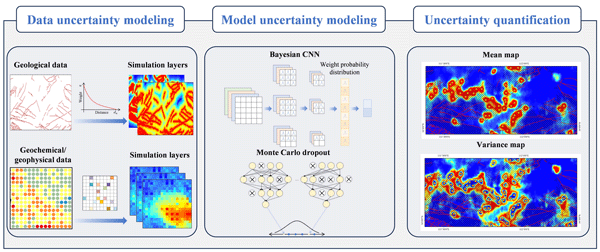
Deep learning algorithms have significantly advanced mineral prospectivity mapping (MPM) by facilitating automated feature extraction and capturing nonlinear relationships among multi-source geological datasets. However, deep learning algorithms for MPM frequently neglect the intrinsic uncertainties arising from incomplete geological knowledge, limited sampling, and model variability, leading to overconfident and potentially unreliable predictions. To address this limitation, this study proposes a comprehensive uncertainty quantification framework that jointly evaluates the input data, model, and predictive uncertainties in deep learning-based MPM. Data uncertainty, originating from limited spatial resolution of geochemical/geophysical features and subjective interpretations of geological information, is characterized through stochastic simulation of evidential layers. Model uncertainty, arising from variability in network architecture and parameters estimation, is captured through a joint Bayesian convolutional neural network (CNN) and Monte Carlo Dropout. Predictive uncertainty, representing the overall uncertainty of predictions, is quantified by integrating the contributions of both data and model uncertainties. The proposed framework is demonstrated through a case study of gold prospectivity mapping in western Henan Province of China. These uncertainties are quantified using statistical measures including mean, variance, and entropy. The obtained results indicate that areas exhibiting high prospectivity and low uncertainty represent robust exploration targets, whereas those with high uncertainty highlight regions requiring improved metallogenic interpretation or model refinement. Furthermore, uncertainty contribution analysis reveals that data uncertainty contributes more to total predictive uncertainty than model uncertainty, suggesting that enhancing the quality and representativeness of evidence layers is more effective for reducing uncertainty than merely optimizing models' architecture or parameters. Overall, by modeling and visualizing both data and model uncertainties, the proposed framework transforms deep learning-based MPM from deterministic prediction to probabilistic decision-making, thereby enabling more reliable and trustworthy mineral exploration.

1 Introduction

Mineral prospectivity mapping (MPM) refers to the application of predictive models to analyze and integrate geological, geochemical, geophysical, and remote sensing datasets for identifying areas that may host undiscovered mineral resources (Bonham-Carter, 1994). Methodologies for MPM have progressed from traditional statistical analysis to machine learning techniques and, more recently, highlight deep learning algorithms as the dominant paradigm (Yang et al., 2024a; Zuo et al., 2025; Lee and Moon, 2026). Compared with traditional approaches, deep learning algorithms are capable of progressively and automatically extracting high-level representations from multi-source geological data, enabling a more comprehensive understanding of complex and nonlinear mineralization processes (Zuo et al., 2019, 2023). A wide range of deep learning techniques has been applied in MPM, including autoencoders (Xiong and Zuo, 2016), convolutional neural networks (CNNs) (Li et al., 2020), generative adversarial networks (Li et al., 2022), graph neural networks (Zuo and Xu, 2023), and recurrent neural networks (Yin et al., 2022). Although these methods offer substantial advantages, however, a critical challenge remains: most deep learning algorithms for MPM overlook inherent sources of uncertainty, resulting in overconfident predictions.

Quantifying uncertainty is a critical task in supporting decision-making for MPM. Bárdossy (2004) defined uncertainty as the recognition that measurements and observations may deviate from natural reality, reflecting the imperfect and incomplete nature of human knowledge. In general, quantifying uncertainty is essential for addressing two key questions: where uncertainty arises and how it can be evaluated (Bárdossy and Fodor, 2001; Burkin et al., 2019). Typically, the workflow of deep learning-based MPM involves: (1) developing a conceptual metallogenic model; (2) collecting and preprocessing multi-source geological data; (3) constructing evidential layers; and (4) integrating these evidential layers using deep learning algorithms to produce a prospectivity map (Carranza, 2008; Zuo, 2020). Due to the multiple interpretations of geological knowledge, limited sampling, observational errors, and biased predictive models, uncertainties may arise at every stage of this workflow (Mann et al., 1994; Kreuzer et al., 2008; McCuaig et al., 2010; Zuo et al., 2021). Moreover, these uncertainties can propagate and accumulate throughout subsequent stages, ultimately leading to unreliable prospectivity predictions.

Uncertainty is commonly categorized into two types: aleatoric and epistemic (Hüllermeier and Waegeman, 2021; Wang et al., 2026). Aleatoric uncertainty, often termed data-related uncertainty, arises from intrinsic noise in data such as limited sampling, measurement errors, and observation inaccuracies. In contrast, epistemic uncertainty, or model-related uncertainty, originates from incomplete knowledge of the prediction model. This study focuses on the quantification of data-related uncertainty, model-related uncertainty, and total predictive uncertainty in MPM. Data uncertainty considers limited spatial resolution, subjective geological interpretations, and the selection of negative samples. Model uncertainty considers the variability in network architecture and parameters used to integrate evidential features. Predictive uncertainty represents the combined influence of these two sources and provides an overall measure of uncertainty in prospectivity predictions.

Mineralization is controlled by the integrated effects of multiple geological processes, and geochemical and geophysical data provide indirect evidence for this process (McCuaig et al., 2010; Hronsky and Kreuzer, 2019). In terms of data uncertainty quantification, existing studies have primarily focused on the construction of evidential features, including ore-controlling geological structures, geochemical anomalies, and geophysical anomalies (Zhang et al., 2024). For geological evidence features (e.g., ore-controlling faults, intrusions, and formation), discretization is often performed by classifying them into categorical units and assigning corresponding weights. Traditional approaches usually assign binary weights (0 or 1) based on the presence or absence of evidential features, thereby introducing uncertainty due to subjective interpretations of mineralization processes (Lisitsin et al., 2014; Yousefi and Carranza, 2015). Improved approaches like fuzzy logic (Knox‐Robinson, 2000) and fuzzy weights of evidence methods (Cheng and Agterberg, 1999) overcome this limitation by assigning continuous weights ranging from 0 to 1, which more realistically represent geological facts. For geochemical and geophysical evidence features, discrete sampling points are typically transformed into continuous grids using interpolation methods such as kriging (Matheron, 1963) and inverse distance weighting (Shepard, 1968). However, when sampling density is low, these interpolation approaches tend to oversmooth the data and can introduce biased estimates in unsampled locations (Goovaerts, 1997). Geostatistical simulation mitigates this limitation by modeling the probability distributions of values in unsampled areas, thereby effectively capturing complex multi-point spatial structures in discrete data and quantifying uncertainty caused by missing data (Wang and Zuo, 2019; Liu et al., 2019).

Additionally, data-driven MPM generally relies on both positive and negative training samples to establish the relationship between predictor variables and mineralization (Carranza et al., 2008). Positive samples are typically derived from known mineral deposit locations. In contrast, negative samples are more challenging to define because the absence of known mineralization does not necessarily indicate the absence of undiscovered deposits (Zuo and Wang, 2020). Consequently, negative samples are commonly constructed from randomly selected background points under geological constraints, known occurrences of other mineral deposit types, or drill holes with economically insignificant mineralization (Nykänen et al., 2015; Lindsay et al., 2022; Montsion et al., 2024). Carranza et al. (2008) further summarized four criteria for generating negative training samples: (1) negative samples should be selected sufficiently far from any known mineral deposit; (2) the number of negative samples should be equal to the number of positive samples; (3) the locations of negative training samples should be selected randomly; (4) the selected negative training sample locations should adequately represent the range of all variables. Previous research has demonstrated that the selection strategy for negative samples can introduce substantial uncertainty and significantly affect the predictive performance of MPM models (Zuo and Wang, 2020; Parsa and Carranza, 2021). Therefore, developing reliable strategies for constructing negative samples remains a critical challenge in MPM.

For model uncertainty quantification, Bayesian neural networks have emerged as one of the most widely used approaches (Gawlikowski et al., 2023). In traditional deep learning algorithms, network parameters are treated as deterministic values optimized during training. Although this approach often yields high predictive accuracy, it can also lead to overconfident and potentially unreliable predictions, especially when dealing with noisy or limited training datasets (Abdar et al., 2021). Bayesian neural networks provide an effective solution to this issue by incorporating probabilistic modeling into the neural network architecture (Wang and Yeung, 2020). Rather than treating network parameters as fixed values, Bayesian neural networks represent them as prior probability distributions, thereby capturing uncertainty by estimating the corresponding posterior distributions (Mena et al., 2021). To approximate the intractable posterior distribution of network parameters, various techniques have been developed, including Markov Chain Monte Carlo (Gilks et al., 1995), variational inference (Blei et al., 2017), and Monte Carlo Dropout (Gal and Ghahramani, 2016). Among them, Monte Carlo Dropout stands out as a practical and computationally efficient method for approximating Bayesian inference (Gal, 2016; Gal and Ghahramani, 2016). Originally introduced as a regularization technique to mitigate overfitting, dropout works by randomly disabling subsets of neurons during the training phase (Srivastava et al., 2014). At inference time, multiple stochastic forward passes are performed with different dropout masks, producing an ensemble of predictions. The variability among these predictions reflects the model uncertainty associated with the network architecture and parameter estimation (Gal and Ghahramani, 2016).

In summary, this study proposes an uncertainty quantification framework for MPM. The framework jointly simulates data uncertainty from evidential layers construction and negative training sample selection, model uncertainty caused by variability in models' architecture and parameters, as well as the resulting predictive uncertainty arising from the combined influence of these two sources. The main contributions are: (1) integrating Monte Carlo Dropout into a CNN to construct a Bayesian deep learning model for MPM; (2) quantifying both data and model uncertainties using statistical measures such as mean, variance, and entropy; (3) performing contribution analyses to evaluate the relative influence of different uncertainty sources on the overall predictive uncertainty. The proposed framework is illustrated through a case study of gold prospectivity mapping in western Henan Province of China, enabling the delineation of more reliable and trustworthy mineral prospective areas based on quantified uncertainties.

2 Methodology

2.1 Data uncertainty modeling

In deep learning-based MPM, ore-controlling features sometimes should be transformed into evidential layers according to mineral deposit models, which are then integrated to predict mineral potential by learning their relationships with known mineralization. However, this process inherently introduces uncertainty due to incomplete understanding of mineralization processes, insufficient spatial resolution for finer modeling grid, and training dataset construction (Zuo et al., 2021). In this study, data uncertainty is represented by stochastic simulation of evidential layers, including geological, geochemical, and geophysical features.

2.1.1 Geological evidential layers simulation: multifractal singularity

Geological evidential layers are commonly constructed by discretizing geological features and transforming them into weighted evidential features using weighting function. This process introduces uncertainty because the weighting functions are typically determined based on geological knowledge and expert judgment rather than objective observations. To simulate the uncertainty associated with this weighting functions, multifractal theory (Cheng and Agterberg, 1996) offers a mathematical foundation. Mineralization can be viewed as a singular geological phenomenon, marked by the localized concentration of energy or matter within a constrained spatiotemporal domain (Cheng, 2007). Under the framework of multifractal singularity theory, the relationship between mineral deposit density (ρ) and the scale (ϵ), defined as the distance to specific geological features, exhibits fractal behavior in two-dimensional space. This relationship can be expressed by a power-law function (Cheng, 2007; Zuo, 2016; Wang and Zuo, 2022):

$$\begin{array}{}\text{(1)}& \mathit{\rho }=c{\mathit{ϵ}}^{-(\mathrm{2}-\mathit{\alpha })},\end{array}$$

where α denotes the singularity index and c is a constant. The singularity index has proven effective for quantifying the spatial association between mineralization and geological features, thereby facilitating the construction of weighting functions for various geological evidential features (Zuo, 2016). A smaller singularity index reflects a stronger association between the corresponding geological features and the mineralization process, indicating greater metallogenic significance. Generally, for a given location (i,j) near a geological feature, areas closer to the feature tend to contain more significant mineralization information and should therefore be assigned higher weights. Conversely, areas farther away are less relevant, or even irrelevant to mineralization, should be assigned lower weights. Accordingly, the weighting function for an evidential feature can be expressed as a piecewise formula (Zuo, 2016; Wang et al., 2020):

$$\begin{array}{}\text{(2)}& {\mathit{\omega }}_{ij}=\left\{\begin{array}{l}c{d}^{-(\mathrm{2}-\mathit{\alpha })}d\le d_{\mathrm{m}}\\ \mathrm{0}d>d_{\mathrm{m}}\end{array},\right.\end{array}$$

where d denotes the distance from a given location (i,j) to the geological feature, d_m represents the maximum effective controlling distances of that feature. The weight ω quantifies the relative contribution of the geological feature to mineralization, with a larger ω indicating stronger ore-controlling effect.

In practice, the weight ω can be estimated by fitting a linear relationship to the log–log plot of ρ versus d using the least-squares method (Zuo, 2016; Wang et al., 2015):

$$\begin{array}{}\text{(3)}& \log \left(\mathit{\rho }\right)=-\mathit{\omega }\log \left(d\right)+c.\end{array}$$

In the Eq. (2), the controlling distance d_m, also known as the spatial extent of a feature's influence, is typically set empirically based on mineral deposit models, which vary according to expert interpretation. This subjectivity inevitably introduces data uncertainty into MPM (Wang and Zuo, 2022). To account for this uncertainty, the parameter d_m is treated as a stochastic variable and randomly sampled within a predefined interval to generate multiple realizations of geological evidential features (Fig. 1). Consequently, the weighting function for geological features is expressed as:

$$\begin{array}{}\text{(4)}& \mathit{\omega }={\displaystyle \frac{\mathrm{1}}{\mathrm{1}-{d_{\mathrm{m}}}^{(\mathrm{2}-\mathit{\alpha })}}}\left(x^{-(\mathrm{2}-\mathit{\alpha })}-d_{\mathrm{m}}\right).\end{array}$$

This formulation accounts for both the relative influence of geological features on mineralization and the uncertainty in the modeling process of evidential feature. The resulting weight values range continuously from 1 and 0. A weight of 1 indicates a strong statistical correlation between the geological feature and known mineral deposits, whereas decreasing values represent weaker spatial association. When the location x exceeds the maximum controlling distances d_m, the weight reduces to 0, implying that the geological feature in those regions exerts no measurable impact on mineralization.

After obtaining the weight ω, the geological evidence layer g_(ω) can be constructed as:

$$\begin{array}{}\text{(5)}& g_{\left(\mathit{\omega }\right)}=g\cdot \mathit{\omega },\end{array}$$

where g is the original gridded geological feature and g_(ω) is the weighted geological evidence layer.

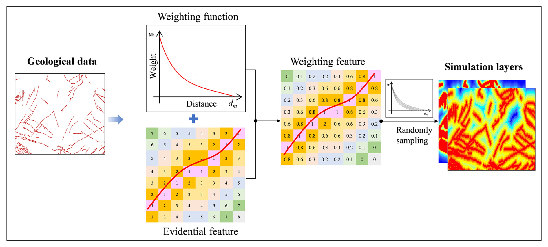
Figure 1 A workflow of geological evidential layer simulation for data uncertainty modeling. Geological data are transformed into weighted evidential features using a distance-decay weighting function, and uncertainty is modeled by randomly sampling the maximum controlling distance to generate multiple simulation layers.

2.1.2 Geochemical and geophysical evidential layers simulation: direct sampling

Grid construction from discrete samples is a fundamental step in generating continuous geochemical and geophysical evidence features. Unlike conventional two-point geostatistical methods, which characterize spatial dependence primarily through pairwise correlations or variograms, direct sampling (DS) multiple-point statistical simulation can reproduce complex spatial patterns involving multiple neighboring locations (Mariethoz et al., 2010; Meerschman et al., 2013). This capability is particularly useful for variables whose spatial distributions may exhibit nonlinear, non-Gaussian, and complex patterns that cannot be adequately represented by two-point statistics alone. In DS, a training image (TI) provides representative spatial patterns and local configurations for simulation, which serves as a reference for multiple-point pattern matching. Unlike conventional geostatistical methods, DS does not require a strict stationary Gaussian assumption. Instead, it searches the TI for patterns that closely resemble the local conditioning data event and reproduces the corresponding patterns to reconstruct values at unsampled locations (Hosseini et al., 2021).

Let G denote the simulation grid, z(x_i) represent the observed value at location x_i, and $D={\left\{(x_i,z\left(x_i\right))\right\}}_{i=\mathrm{1}}^n$ belongs to the set of n conditioning data. The goal of DS is to estimate z(x) for all unsampled locations x. At each unsampled node, a data event is defined as the set of conditioning nodes within a specified neighborhood around x. In the training image TI, DS commonly employs the normalized mean squared error to quantify the similarity between the simulation data event and the TI pattern. Given a similarity threshold t, DS sequentially scans the TI until the distance between an observed data event and a TI pattern falls below the threshold t. Then, the value at the central node of the matched TI pattern is assigned to the simulation node. If no sufficiently similar pattern is found after scanning a maximum fraction f of the TI, the value from the best-matched pattern encountered is used instead. By iteratively applying this procedure, DS generates multiple realizations, each honoring the conditioning data but differing in local spatial details due to stochastic sampling. This process transforms discrete samples into gridded maps that, on the one hand, alleviate smoothing effects at unsampled locations and, on the other hand, incorporate uncertainty arising from data gaps and limited spatial resolution (Yang et al., 2023; Wang et al., 2023) (Fig. 2).

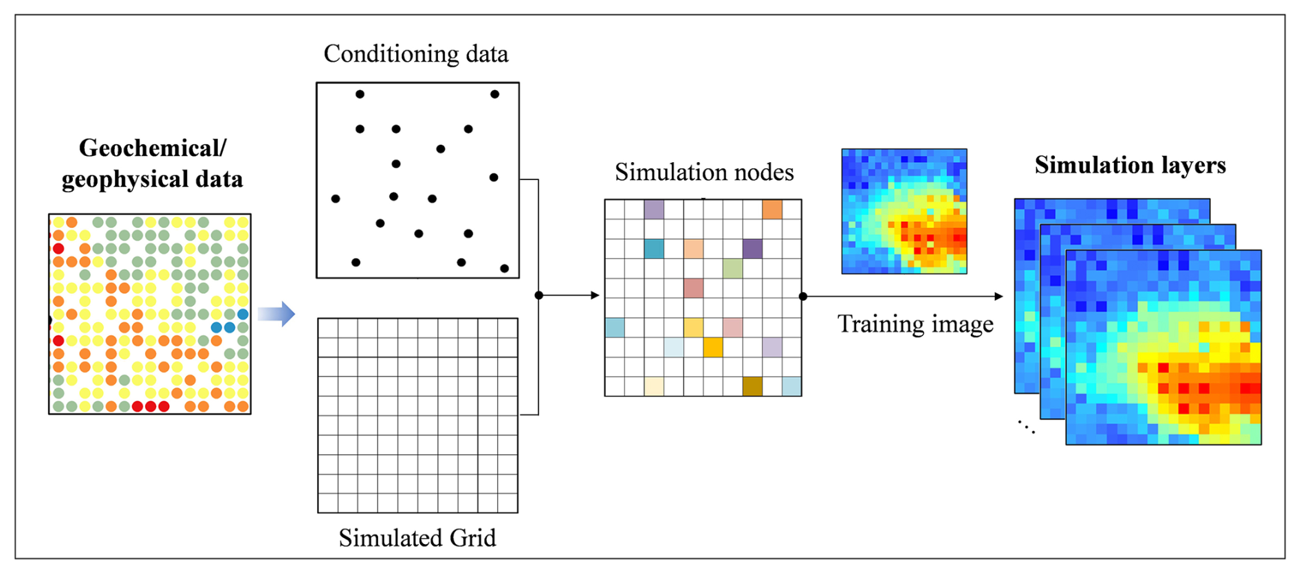
Figure 2 A workflow of geochemical and geophysical evidential layer simulation for data uncertainty modeling. Discrete observations are used as conditioning data, while the original gridded evidential layer serves as TI. For each unsampled node, DS algorithm sequentially scans the TI to find the best-matching local pattern and assigns its central value, generating multiple stochastic realizations that preserve spatial continuity and represent data uncertainty.

2.2 Negative training samples: random generation

CNNs rely on both positive and negative samples to learn discriminative features that distinguish mineralization from non-mineralized backgrounds. In practice, known mineral deposit locations are used as positive samples, while negative samples are typically selected randomly from non-mineralized areas (Carranza et al., 2008). However, the definition of non-mineralized regions is inherently uncertain, as geological processes are continuous and ore-forming environments may extend beyond the boundaries of known mineral deposits. In this study, the uncertainty associated with negative samples selection is modeled by randomly sampling points from regions located at least 10 km from known mineral deposits, ensuring minimize potential mineralization influence. The 10 km exclusion distance was determined empirically based on the geological characteristics of the study area and is consistent with the maximum mineralization control distance adopted in this study. The effects of negative sample selection on model performance can then be quantified, thereby providing a measure of data uncertainty arising from training sample preparation (Zuo and Wang, 2020).

2.3 Model uncertainty modeling

2.3.1 Bayesian CNN

CNNs can automatically extract low-level features, which are progressively combined into higher-level representations describing complex spatial patterns (Gu et al., 2018). A standard CNN architecture comprises a sequence of convolutional, pooling, and fully connected layers. The convolutional layers are responsible for capturing local spatial patterns using learnable filters; the pooling layers downsample feature maps, thereby lowering computational cost and helping to prevent overfitting. The fully connected layers then aggregate the extracted features into a global representation for final prediction. This hierarchical progression from low-level to high-level feature representations makes CNNs particularly effective for integrating diverse spatial evidential layers in MPM.

Bayesian CNNs (Fig. 3a) extend traditional CNNs by incorporating Bayesian inference to model uncertainty in both network parameters and predictions (Gal and Ghahramani, 2015; Shridhar et al., 2019). Bayesian CNNs share similar architectures with standard CNN while treat network weights as random variables defined by probability distributions. This probabilistic framework enables the network to learn complex, nonlinear feature representations while simultaneously quantifying model uncertainty. During training, Bayesian inference approximates the posterior distribution of network parameters. At inference time, multiple stochastic forward passes are conducted to produce a distribution of predictions, thereby enabling the estimation of model uncertainty.

2.3.2 Monte Carlo dropout

Bayesian inference provides a theoretical framework for modeling parameter uncertainty and propagating it into model uncertainty. However, exact Bayesian inference in neural networks is intractable due to high-dimensional parameter spaces. Monte Carlo Dropout is a practical and computationally efficient means to approximate Bayesian inference, without explicitly learning probability distributions over network weights (Gal and Ghahramani, 2016; Seoh, 2020) (Fig. 3b). Originally introduced as a regularization technique, dropout works by randomly deactivating neurons during training with a specified probability. In the Bayesian interpretation, this process can be viewed as sampling from a distribution over network parameters. During inference, dropout is kept active and multiple stochastic forward passes are performed for the same input, each corresponding to a different thinned subnetwork. The resulting ensemble of predictions forms an approximate posterior predictive distribution, enabling the estimation of model uncertainty. Importantly, Monte Carlo Dropout provides a lightweight, scalable, and easily implementable approach to Bayesian deep learning by simply adding dropout layers before each pooling layer in a standard CNN architecture.

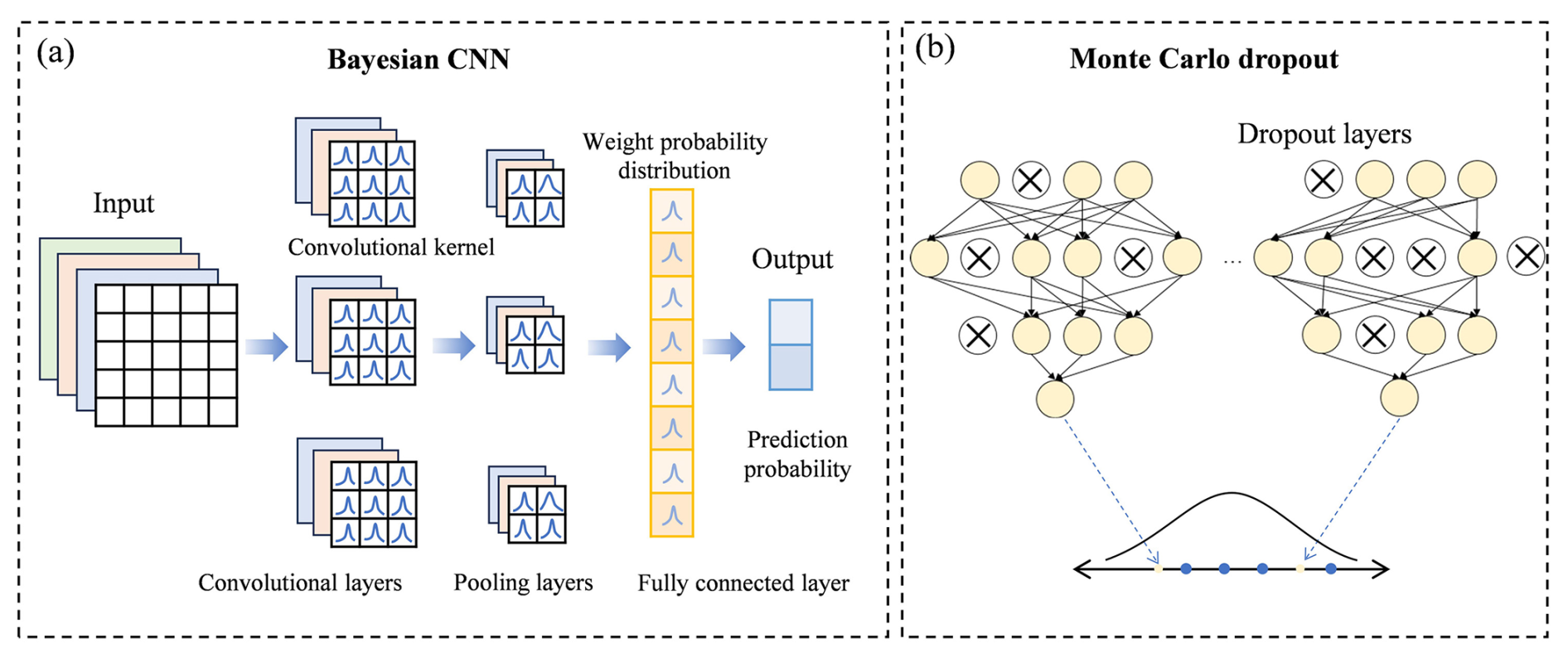
Figure 3 A workflow of model uncertainty modeling: (a) Bayesian CNN, (b) Monte Carlo dropout. Model uncertainty is quantified by treating network weights probabilistically in a Bayesian CNN. Bayesian inference is approximated using Monte Carlo dropout by activating dropout during inference and performing multiple stochastic forward passes to estimate uncertainty.

2.4 Uncertainty quantification metrics

For uncertainty quantification, variance and entropy are two of the most widely used statistical measures. Given T stochastic predictions ${\left\{p_t\right\}}_{t=\mathrm{1}}^T$, where p_t is the probability predicted by the Bayesian CNN, the variance can be expressed as:

$$\begin{array}{}\text{(6)}& \mathrm{Var}\left(p\right)={\displaystyle \frac{\mathrm{1}}{T}}\sum _{t=\mathrm{1}}^T(p_t-\stackrel{\mathrm{‾}}{p}{)}^{\mathrm{2}},\end{array}$$

where $\stackrel{\mathrm{‾}}{p}$ denotes the mean prediction across all T forward passes at each location (i,j). Variance reflects the dispersion of predictions around the mean, indicating the degree of disagreement among stochastic realizations.

Entropy, introduced by Shannon (1948) in information theory, measures the expected amount of information contained in a probability distribution. It has been extensively applied in geoscientific modeling to characterize uncertainty in spatial predictions (Wellmann and Regenauer-Lieb, 2012). Mathematically, entropy is defined as (Shannon, 1948):

$$\begin{array}{}\text{(7)}& H\left(p\right)=-\sum _{t=\mathrm{1}}^T{p}_t\log p_t.\end{array}$$

In this study, entropy quantifies the expected uncertainty of the predicted probability distribution for mineral occurrence. Thus, a higher entropy value indicates a more diffuse probability distribution, reflecting greater uncertainty and a lower level of confidence in the predicted prospectivity map.

3 Study area and dataset

3.1 Geological setting

The case study area is situated in western Henan Province of China (Fig. 4). This region is recognized as one of the country's most important gold-producing areas, hosting more than 81 large to super-large size of gold deposits (Deng and Wang, 2016; Fan et al., 2016; Zhang et al., 2020). Such findings highlight substantial potential for further gold exploration (Mao et al., 2002a; Mao, 2005; Tang et al., 2013). These gold deposits are predominantly magmatic-hydrothermal in origin, formed mainly during the Early Cretaceous under an extensional tectonic regime of the Yanshanian period (Mao et al., 2002b). According to the established mineral deposit models (Wu et al., 2012), mineralization and its spatial distribution are primarily controlled by regional faults, Yanshanian intrusions, and the strata of the Xiong'er and Taihua rock groups. Specifically, ore-forming materials are sourced from the deep mantle, while intrusions of intermediate to acidic magmatic rocks supplied the thermal energy for fluid migration. Faults served as major conduits for fluid transport, ultimately leading to gold mineralization within the Taihua and Xiong'er Group formations (Lu et al., 2002; Pang et al., 2020).

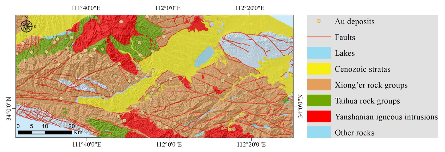
Figure 4 A simplified geological map of the study area (modified from the Geological Survey Institute of Henan, China).

3.2 Dataset

Geochemical and aeromagnetic data provide indirect indicators or proxy evidence of regional geophysical and elemental anomalies linked to gold mineralization. The geochemical exploration dataset was sourced from the Chinese National Geochemical Mapping Project (Xie et al., 1997), comprising of 1131 stream sediment samples collected at a 1:200 000 scale. The original stream sediment geochemical data were conducted at an average density of one sample per 1 km², after which four adjacent samples were composited to represent a 4 km² area grid cell (Xie et al., 1997). Each sample contains concentrations of 39 major and trace elements, determined using analytical techniques such as inductively coupled plasma atomic fluorescence spectrometry, X-ray fluorescence, and inductively coupled plasma atomic emission spectrometry (Xie et al., 1997). Geochemical exploration data are typical compositional data, which can induce spurious spatial and statistical correlations among elements (Zuo et al., 2013). Accordingly, geochemical exploration data were preprocessed using the centered-log ratio transformations to eliminate the influence of closure effects (Aitchison, 1982). The geophysical data were acquired from the China Geological Survey, comprising aeromagnetic gridded raster at the same scale. To reduce distortions associated with skewed magnetization, the vertical first-order derivatives were applied to enhance shallow magnetic anomaly signatures. The resulting raster was subsequently used as the geophysical input for simulation. Consequently, 44 mineralization-related evidential features, including faults, Yanshanian intrusions, Xiong'er and Taihua rock groups strata, geophysical aeromagnetic data, and geochemical data, are extracted to construct the evidential layers for MPM (Fan et al., 2023; Yang and Zuo, 2024; Yang et al., 2024b).

4 Evidential layers simulation

4.1 Geological evidential layers simulation

The generation of geological evidence layers relies on buffer analysis combined with weighting functions. This procedure involves counting the number of mineral deposits that fall within different buffer zones surrounding geological features, thereby quantifying their spatial correlation with mineralization. The resulting spatial correlation patterns are subsequently used to derive weighting functions for corresponding evidence layers. Specifically, singularity indexes α are calculated from log–log plots of paired datasets [ρ,d], yielding values of 1.324, 1.74, 1.093, and 1.37 for faults (Fig. 5a), Yanshanian intrusions (Fig. 5b), and the Xiong'er (Fig. 5c) and Taihua (Fig. 5d) rock groups strata, respectively. Fractal analysis suggests that the Xiong'er group strata and faults exert a stronger spatial influence on gold mineralization compared with other geological features. This finding is consistent with established mineral deposit models and existing geological knowledge (Wu et al., 2012), thereby supporting the reliability of the geological evidence layer construction.

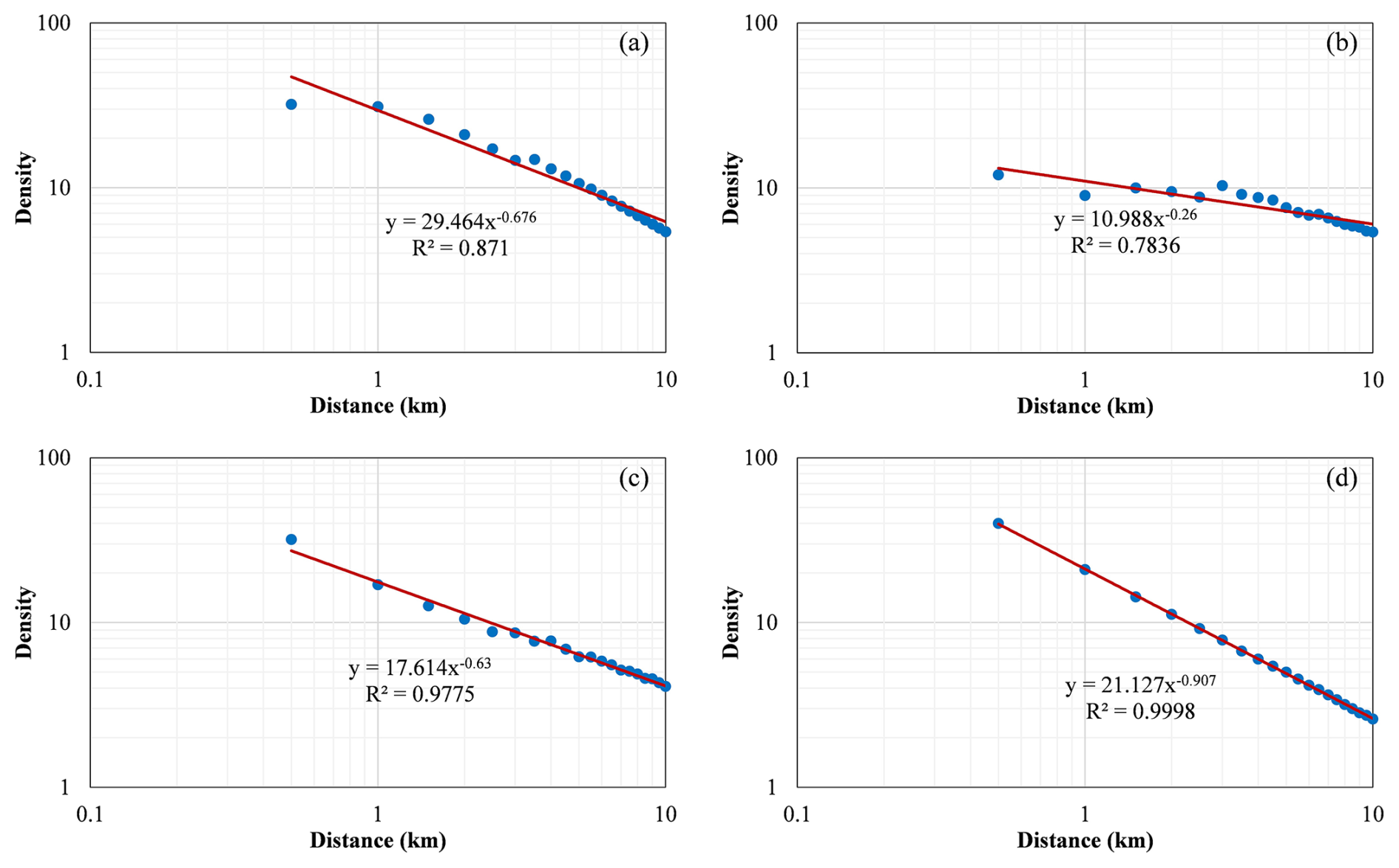
Figure 5 Log–log plots of deposits density vs. buffer width: (a) faults, (b) Yanshanian intrusions, (c) Taihua rock groups strata, and (d) Xiong'er rock groups strata.

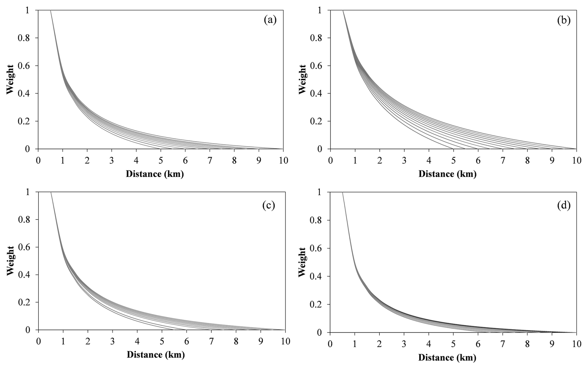
Figure 6 Weighting functions curves: (a) faults, (b) Yanshanian intrusions, (c) Taihua rock groups strata, and (d) Xiong'er rock groups strata.

The uncertainty of geological evidential features can be modeled by randomly sampling the parameter d_m within a predefined interval. In this study, the uncertain d_m, representing the maximum controlling distance of a geological feature, is empirically assigned as a random value within the estimated interval [5, 10]. Accordingly, Monte Carlo sampling is performed by randomly selecting d_m values from the defined intervals, generating 100 weighting functions (Fig. 6) and corresponding weighted evidential layers for each geological feature (Fig. 7). These multiple realizations not only capture the variability arising from weighting function but also provide a probabilistic representation of the spatial relationships between geological features and mineralization, thereby offering a more robust characterization of data uncertainty.

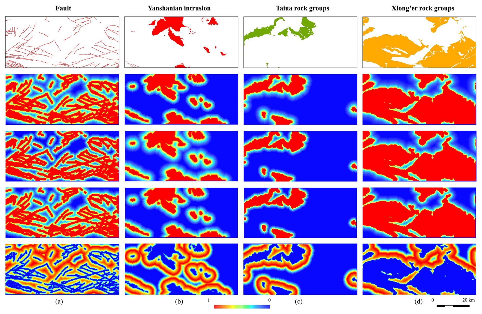
Figure 7 Weighted evidence layers: (a) faults, (b) Yanshanian intrusions, (c) Taihua rock groups strata, and (d) Xiong'er rock groups strata. The first row is the original geological features, the second to fourth rows are the weighted evidence layers. The fifth row is the standard deviation of the generated evidence layer, which clearly illustrates the spatial variability among the realizations.

4.2 Geochemical and geophysical evidential layers simulation

To model the spatial distribution patterns of geochemical elements, the DS algorithm is employed to transform discrete geochemical measurements into spatially continuous evidential layers on a 500 m grid from the original 2 km scale. This enhancement in spatial resolution inevitably introduces data uncertainty associated with the estimation of unsampled locations. In this study, geochemical layer serves as both conditioning data and the TI for the simulation process. Two parameters, the similarity threshold t and the maximum fraction f of the TI to be scanned, are empirically set to 0.1 and 0.7, respectively. In this regard, a total of 100 realizations of geochemical maps are generated with a spatial resolution of 500 × 500 m, each representing an independently simulated distribution pattern of element concentrations. These multiple simulations infill unsampled locations while preserving the spatial structures of the original datasets. The spatial distribution of Au geochemical samples and three randomly selected simulated evidential layers are shown in Fig. 8a. Geophysical evidence layers are produced following the same simulation procedure. Figure 8b presents three representative simulated aeromagnetic evidence layers.

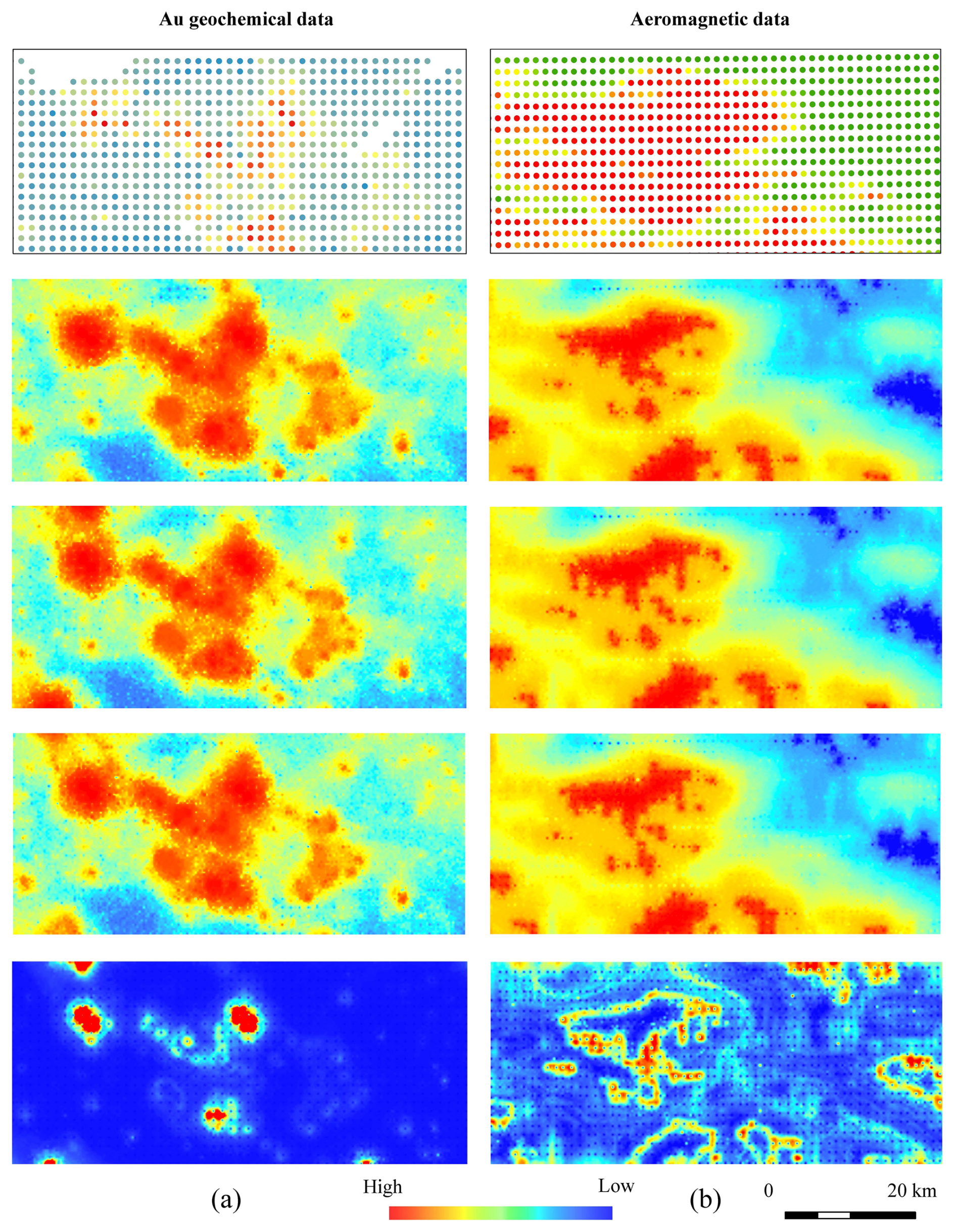
Figure 8 Simulated evidence layers: (a) Au geochemical layer, (b) aeromagnetic layer. The first row is the original geochemical and geophysical data, the second to fourth rows are the DS realizations. The fifth row is the standard deviation of all realizations, which illustrates the spatial variability among the simulated layers.

Furthermore, to evaluate the reliability of the simulated realizations, cumulative frequency distribution and experimental variogram curves are employed to compare the similarity between observed and simulated patterns. Using Au as an example, the cumulative frequency distribution curve (Fig. 9a) clearly demonstrate that the DS reproduces the statistical distribution pattern of geochemical features in the study area. Experimental variograms, which characterize the spatial continuity and autocorrelation of geoscientific data, are used to assess the preservation of spatial structure. The close agreement between the variogram curves of the observed and simulated realizations (Fig. 9b) further indicates that the DS approach successfully reproduces the major spatial structures of the original geochemical layer. These results demonstrate that the simulations preserve not only the statistical distribution of the evidential layers but also their spatial dependence, enabling the generation of realistic geochemical evidence layers while simultaneously accounting for uncertainty associated with unsampled regions.

It is worth noting that the application of DS to geochemical and geophysical data also has limitations. These variables are generally continuous and may exhibit anisotropy and heterogeneous spatial characteristics, which may not be fully represented by a single TI. Consequently, the quality and representativeness of the TI can strongly influence the simulated realizations. Moreover, when DS is applied to pre-interpolated geophysical data, the resulting simulations may inherit part of the smoothing effects and spatial assumptions introduced during the initial interpolation, thereby potentially propagate interpolation-related bias into the simulated realizations.

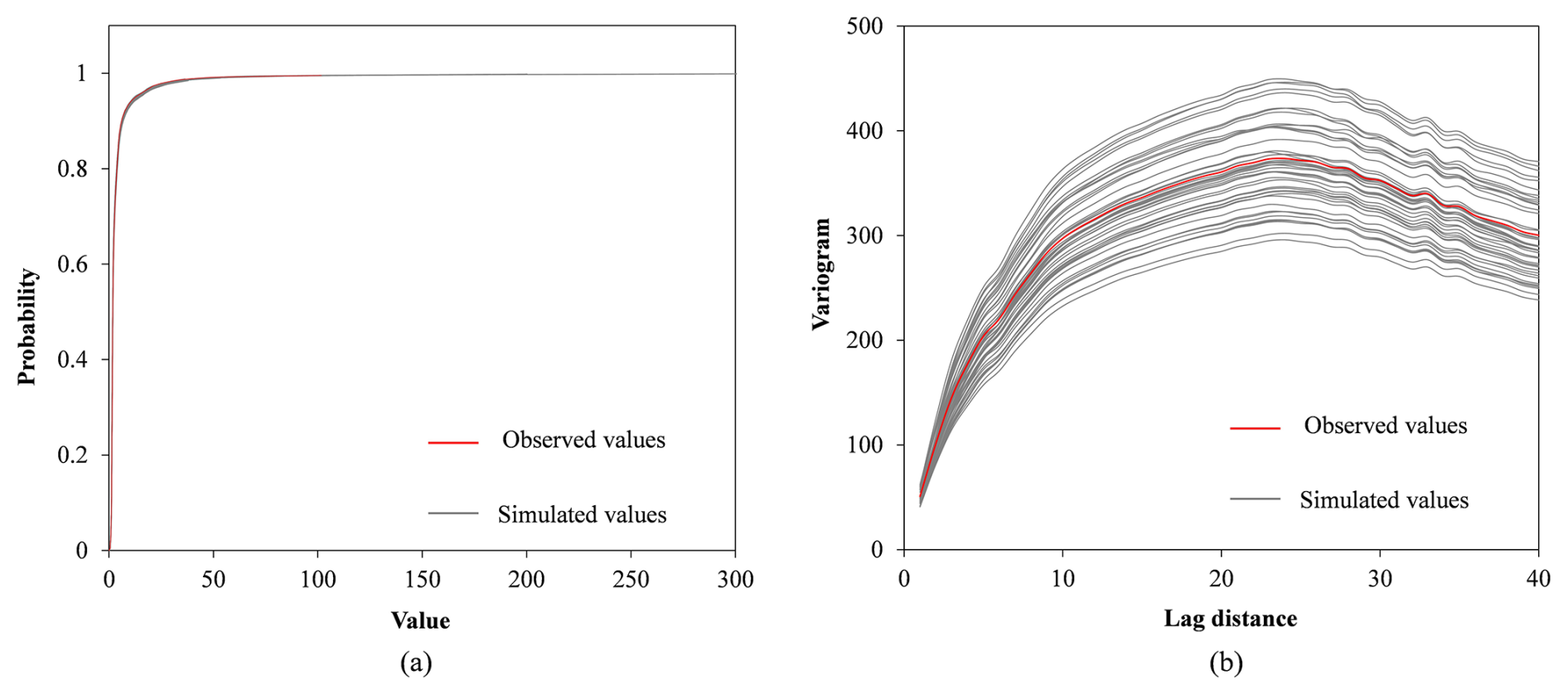
Figure 9 Cumulative frequency distribution curves (a) and experimental variogram curves (b) derived from 100 simulated Au geochemical layers.

In total, 44 evidence layers are constructed as model inputs, including geological features (faults, intrusions, strata), aeromagnetic data, and geochemical data comprising 39 elemental concentration maps. Each evidential layer is simulated 100 times, providing sufficient realizations to quantify data-related uncertainty in MPM.

5 Experimental setting

5.1 Network architecture and parameters

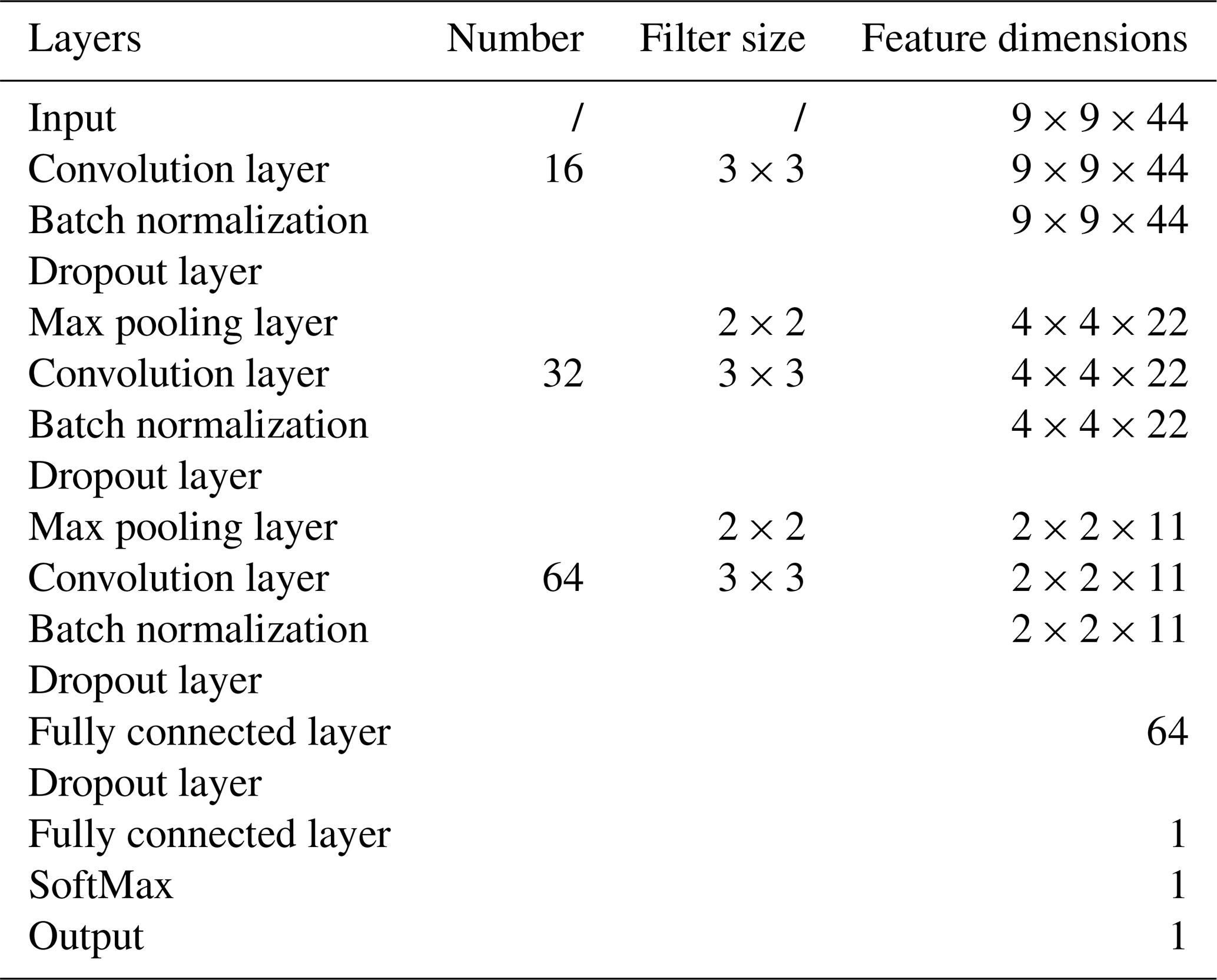
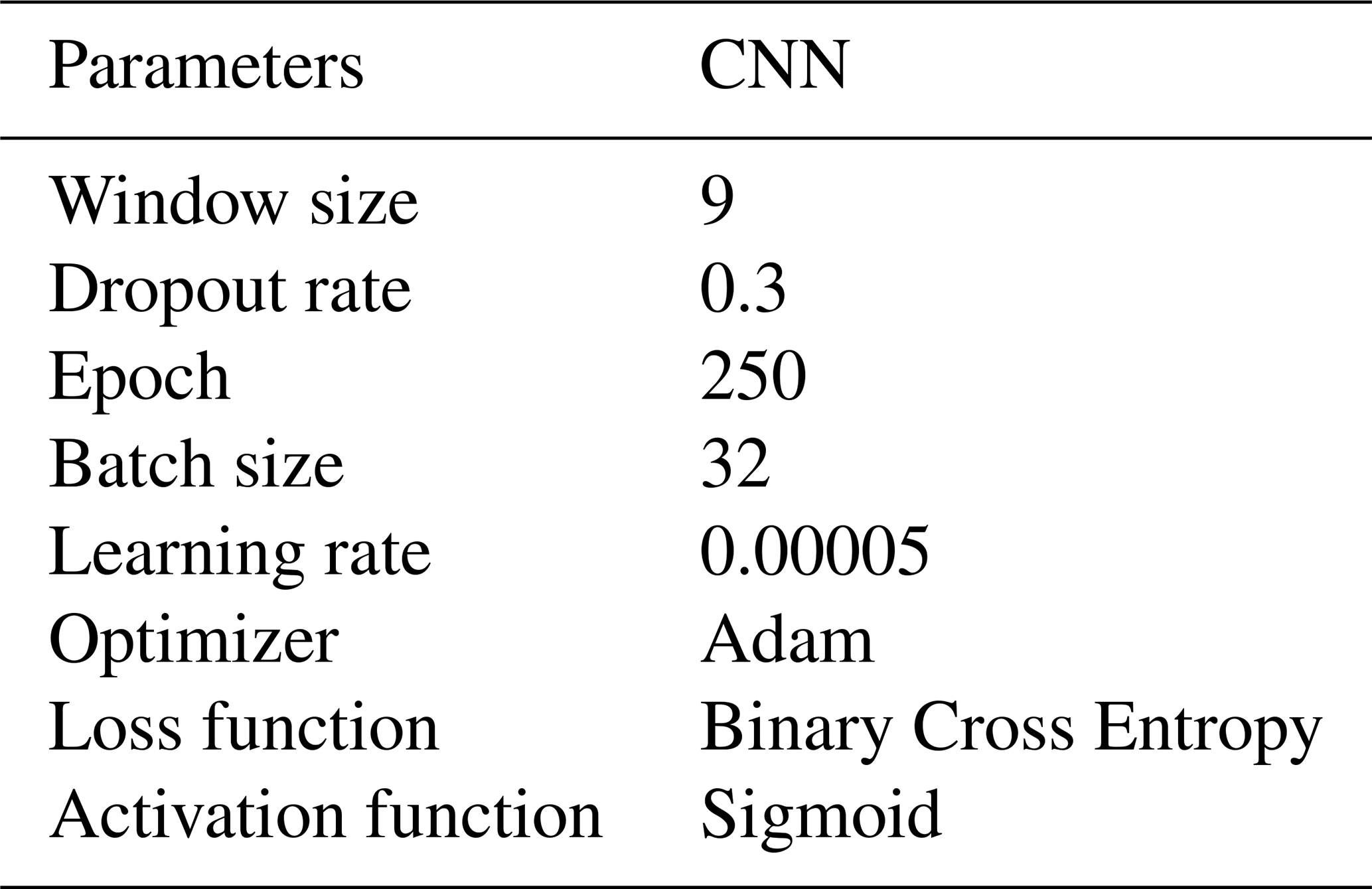
The Bayesian CNN architecture (Table 1) comprises three 3×3 convolutional layers, three normalization layers, two 2×2 max-pooling layers, and two fully connected layers. Each convolutional layer is followed by a dropout layer to facilitate uncertainty estimation. The final output layer employs a sigmoid activation function to produce probability predictions for MPM. Key hyperparameters, including the learning rate, batch size, number of epochs, activation function, and optimizer, are listed in Table 2. These parameters are adjusted through grid search (Liashchynskyi and Liashchynskyi, 2019). Model performance is evaluated using binary cross-entropy loss and classification accuracy. It should be noted that the sensitivity analysis of these parameters is beyond the scope of the present study.

Table 1 Network architecture of the Bayesian CNN.

Table 2 Hyperparameter settings of the Bayesian CNN.

5.2 Sample preparation

A 9 × 9 sliding window is used to draw training samples from the evidential layers. This approach ensures that each training sample encompasses not only the central pixel but also the contextual information from its surrounding 9 × 9 neighborhood. Within this window, each pixel is characterized by 44 evidential features derived from geological, geochemical, and geophysical datasets, forming a comprehensive feature space that enables CNN to learn spatial-attribute relationships associated with mineralization. A total of 483 positive samples with dimensions of 9 × 9 × 44 are extracted from 51 known gold mineral deposits and their surrounding neighborhoods within a 3 × 3 km radius. This data augmentation strategy has been demonstrated effectively to improve the generalization ability of deep learning algorithms in MPM (Li et al., 2022; Zuo, 2025). To ensure dataset balance, an equal number of negative samples are also randomly generated from areas distant from known mineralization during each training stage. Of the total samples, 80 % are used for model training, while the remaining 20 % are reserved for validation.

6 Results

This study proposes a framework to quantify and visualize uncertainty in MPM by modeling data uncertainty via stochastic simulation of evidence layers and model uncertainty via Monte Carlo dropout. To evaluate the influence of different uncertainty sources on MPM, four comparative experimental models are designed: (1) deterministic CNN, (2) data uncertainty quantification, (3) model uncertainty quantification, and (4) total predictive uncertainty quantification that integrates both data and model uncertainties. Each case is structured to isolate or combine specific sources of uncertainty while keeping all other factors constant, allowing a systematic assessment of how data uncertainty, model uncertainty, and their combination affect predictive stability. All cases adopt identical network architectures, parameters, and evaluation metrics to ensure fair comparison.

6.1 Deterministic CNN

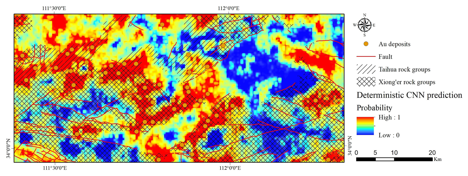
A deterministic CNN is first trained using the original evidence layers to validate the effectiveness of the proposed model's architecture and parameters settings. The training convergence curves of loss and accuracy over epochs (Fig. 10) indicate that the deterministic model achieved stable and satisfactory training performance. The resulting prospectivity map of gold deposits (Fig. 11) reveals that high-potential areas closely align with the spatial distribution of known mineral deposits. The outcomes provide additional evidence supporting the reliability and efficacy of the proposed CNN architecture for MPM.

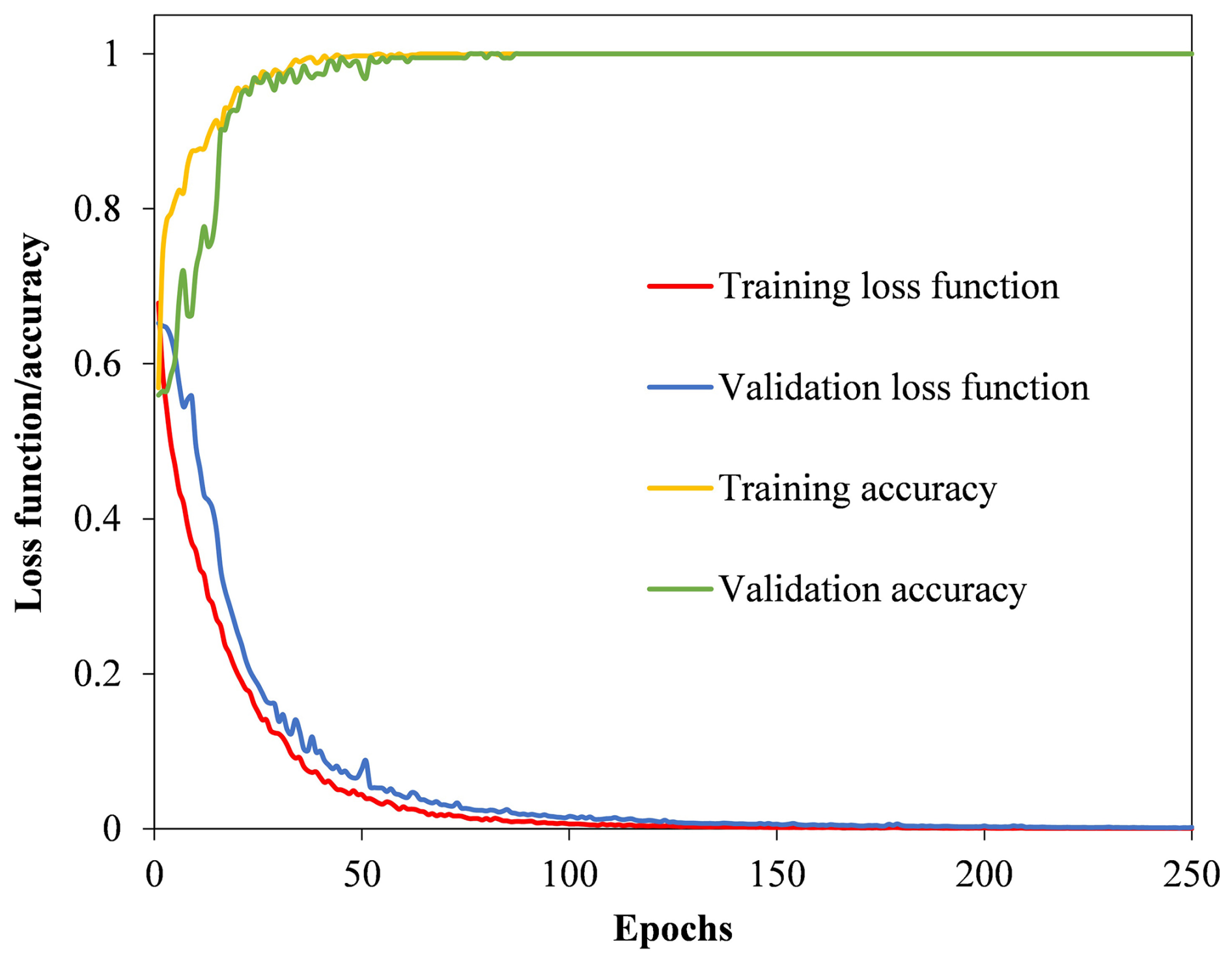
Figure 10 Convergence curves of training loss and accuracy across epochs for the deterministic CNN.

Figure 11 Mineral prospectivity map obtained by the deterministic CNN.

6.2 Data uncertainty quantification

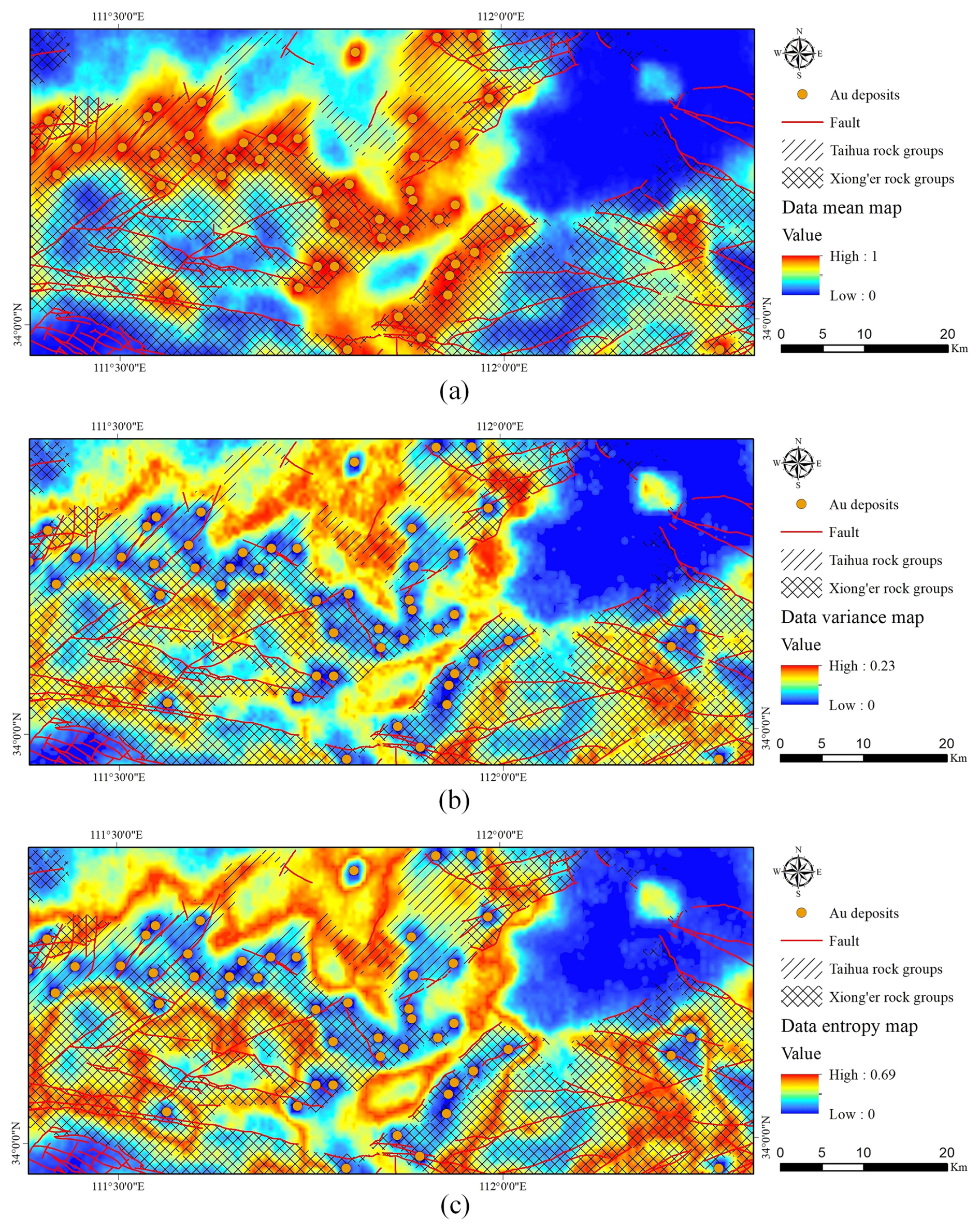
Data uncertainty is quantified by generating multiple simulated evidence layers with randomly selected negative samples, thereby capturing variability arising from incomplete geological knowledge, relatively coarse spatial resolution, and randomness of training labels. A deterministic CNN model is trained on simulated evidence layers to produce 100 prospectivity predictions. Figure 12 presents the mean, variance, and entropy maps across these predictions. The mean map (Fig. 12a) represents the most probable spatial distribution of mineralized potential by averaging the ensemble predictions. High mean values indicate areas of consistently high prospectivity, which are primarily distributed along major faults and within the Xiong'er rock groups strata. These regions closely coincide with known gold mineral deposits, confirming that CNN model effectively captures the key mineralization patterns. Most gold deposits in the study area are quartz-vein and altered-rock types (Mao et al., 2002b), mainly controlled by faults which act as pathways for mineralizing fluids, while the surrounding strata provide favorable host environments, jointly contributing to the high prospectivity in these regions.

The variance and entropy maps reveal different aspects of data uncertainty induced by the stochastic simulation of evidence layers. The variance map (Fig. 12b) quantifies the degree of variability among the 100 prospectivity predictions under varying evidence inputs. Regions with low variance indicate stable predictions and high confidence. Conversely, areas with high variance demonstrate strong sensitivity to data perturbations, suggesting that small variations in evidence layers can substantially affect the predicted probabilities. Although both metrics display broadly similar spatial patterns, the entropy map (Fig. 12c) offers additional insight beyond variance by characterizing the uncertainty in the probability distribution of predictions. In other words, entropy captures the degree of ambiguity in predictions, even when the magnitude of variation is moderate. Overall, areas exhibiting high mean and low entropy values represent the most reliable exploration targets, while those characterized by high prospectivity but high uncertainty deserve further geological investigation.

Figure 12 Data uncertainty quantification: (a) mean, (b) variance, and (c) entropy maps.

6.3 Model uncertainty quantification

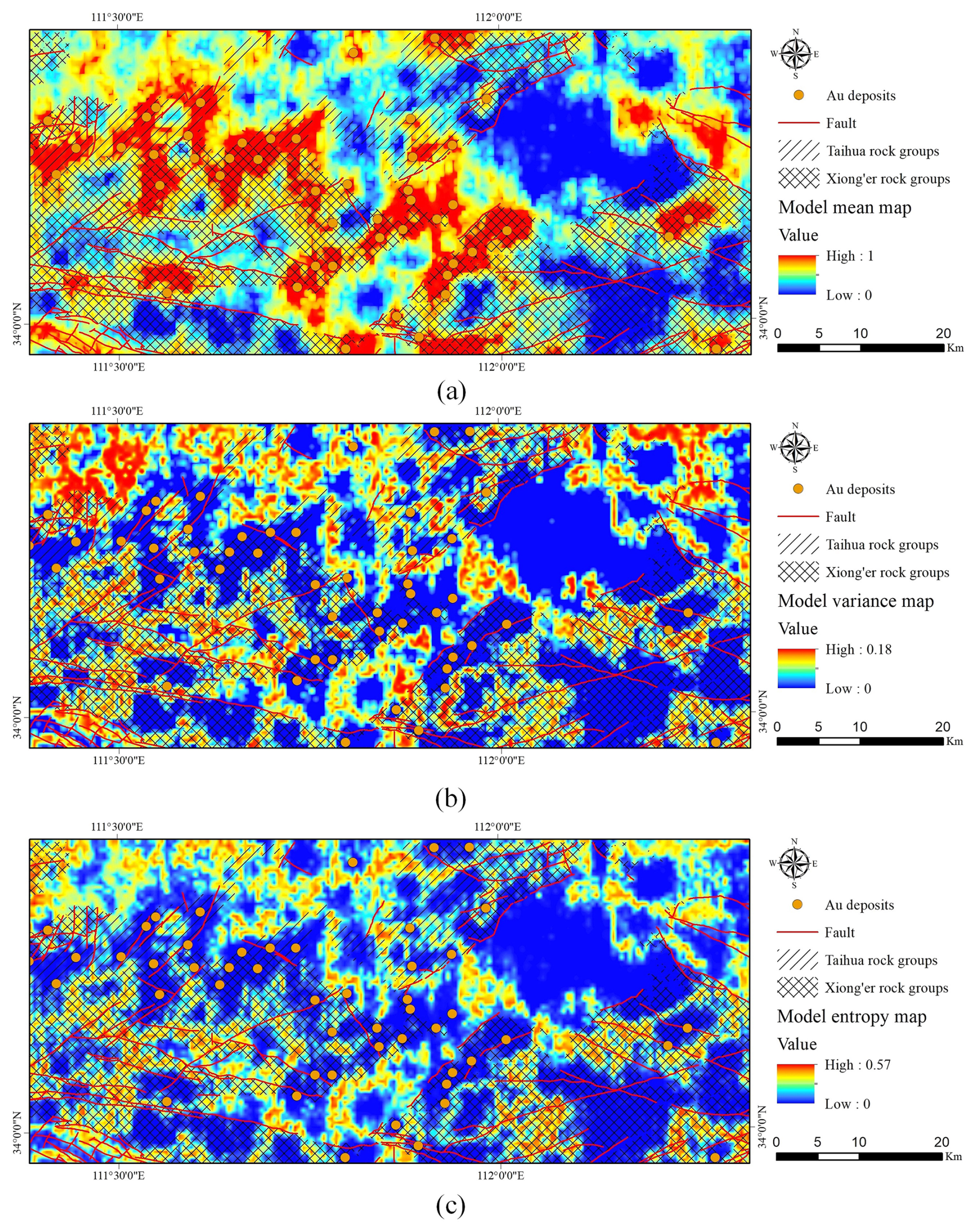
Model uncertainty is quantified using the Bayesian CNN trained on the original evidence layers, reflecting the inherent randomness in network architecture and parameters estimation. The resulting mean, variance, and entropy maps (Fig. 13) provide a comprehensive view of both predictive outcomes and the associated uncertainty in deep learning-based MPM. High-probability regions in the mean map (Fig. 13a) appear primarily distributed within the Xiong'er rock groups, implying favorable conditions for gold mineralization. The strong spatial correspondence between high-probability regions and known gold mineral deposits confirms that the Bayesian CNN model effectively captures the principal ore-controlling geological features of gold mineralization. The variance (Fig. 13b) and entropy maps (Fig. 13c) exhibit similar spatial patterns. Areas with low variance and low entropy generally coincide with high mean probabilities and known gold mineral deposits, reflecting strong model confidence and stable predictive behavior. Conversely, regions with high variance and entropy indicate greater model uncertainty, implying limited model knowledge or insufficient feature representation for inferring mineralization potential in those regions.

Notable differences are observed between the data and model uncertainty maps. Data uncertainty primarily arises from the heterogeneity and stochasticity of evidential layers, whereas model uncertainty reflects the limitations of the network in learning stable and generalizable relationships from the data. Overall, data uncertainty appears broader and more pronounced than model uncertainty, implying that variability in the evidence layers exerts a greater influence than model's architecture or parameter settings. This finding further suggests that, in geologically complex regions, CNN model faces challenges in accurately interpreting gold prospectivity when the input data themselves are highly uncertain.

Figure 13 Model uncertainty quantification: (a) mean, (b) variance, and (c) entropy maps.

6.4 Predictive uncertainty quantification

The total predictive uncertainty represents the combined effects of both data and model uncertainties, derived through stochastic simulation of evidence layers with a Monte Carlo dropout-based Bayesian CNN. Specifically, 100 stochastic realizations of the evidence layers are generated to characterize data uncertainty. For each realization, 100 Monte Carlo Dropout stochastic forward passes were performed to sample model uncertainty. In this way, 10 000 predictions are generated, enabling a comprehensive characterization of the total uncertainty. The mean, variance, and entropy maps are shown in Fig. 14. Compared with the individual uncertainty quantification, the joint consideration of data and model uncertainties yields smoother and more spatially coherent patterns that align better with the distribution of known gold mineral deposits. The mean prospectivity map (Fig. 14a) preserves the main high-prospectivity areas identified in the data and model uncertainties, highlighting the stabilizing effect achieved by combining model stochasticity with variations in evidential inputs. The variance map (Fig. 14b) indicates that the total predictive uncertainty effectively captures variability arising from both geological features and CNN model, thereby enhancing predictive robustness. The spatial distribution of predictive entropy (Fig. 14c) provides direct implications for exploration strategy and model refinement. High entropy regions suggest either input data or model limitations, whereas low entropy areas represent priority targets because the model provides a low-risk predictive indication. Importantly, multiple predictions allow the model to account for variations in both evidence layers and network architecture, resulting in highly consistent variance and entropy patterns across the study area.

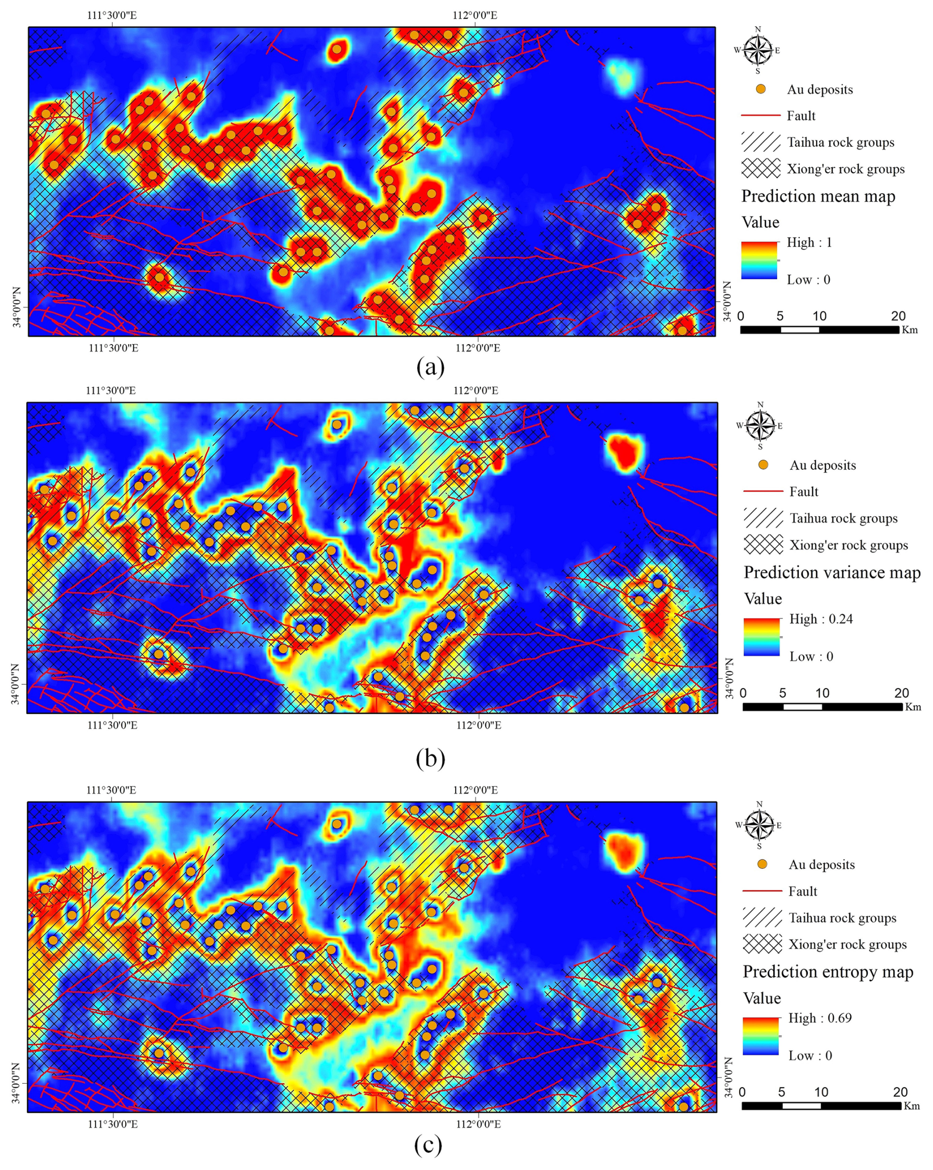
Figure 14 Predictive uncertainty quantification: (a) mean, (b) variance, and (c) entropy maps.

7 Discussion

Uncertainty quantification has become an increasingly important component of deep learning-based MPM. Currently, existing studies primarily focused on uncertainty associated with parameters optimization, network architecture, or prediction models selection using approaches such as Bayesian neural networks and ensemble learning (Daviran et al., 2025; Hoseinzade et al., 2025; Nwaila et al., 2026; Liu, 2025, 2026). Although these methods provide valuable measures of predictive confidence, they generally assume that the input evidential layers are deterministic. In practice, the construction of geological, geochemical, and geophysical evidential layers is subject to substantial uncertainty. Neglecting these sources of uncertainty may result in unreliable prospective predictions. The proposed framework in this study addresses this limitation by integrating uncertainty quantification for both the input evidential layers and the predictive model. By transforming uncertainty from the evidential layers to the final prospective predictions, the proposed approach provides a more comprehensive characterization of predictive uncertainty throughout the entire MPM workflow than approaches relying solely on model uncertainty estimation.

7.1 Uncertainty decomposition

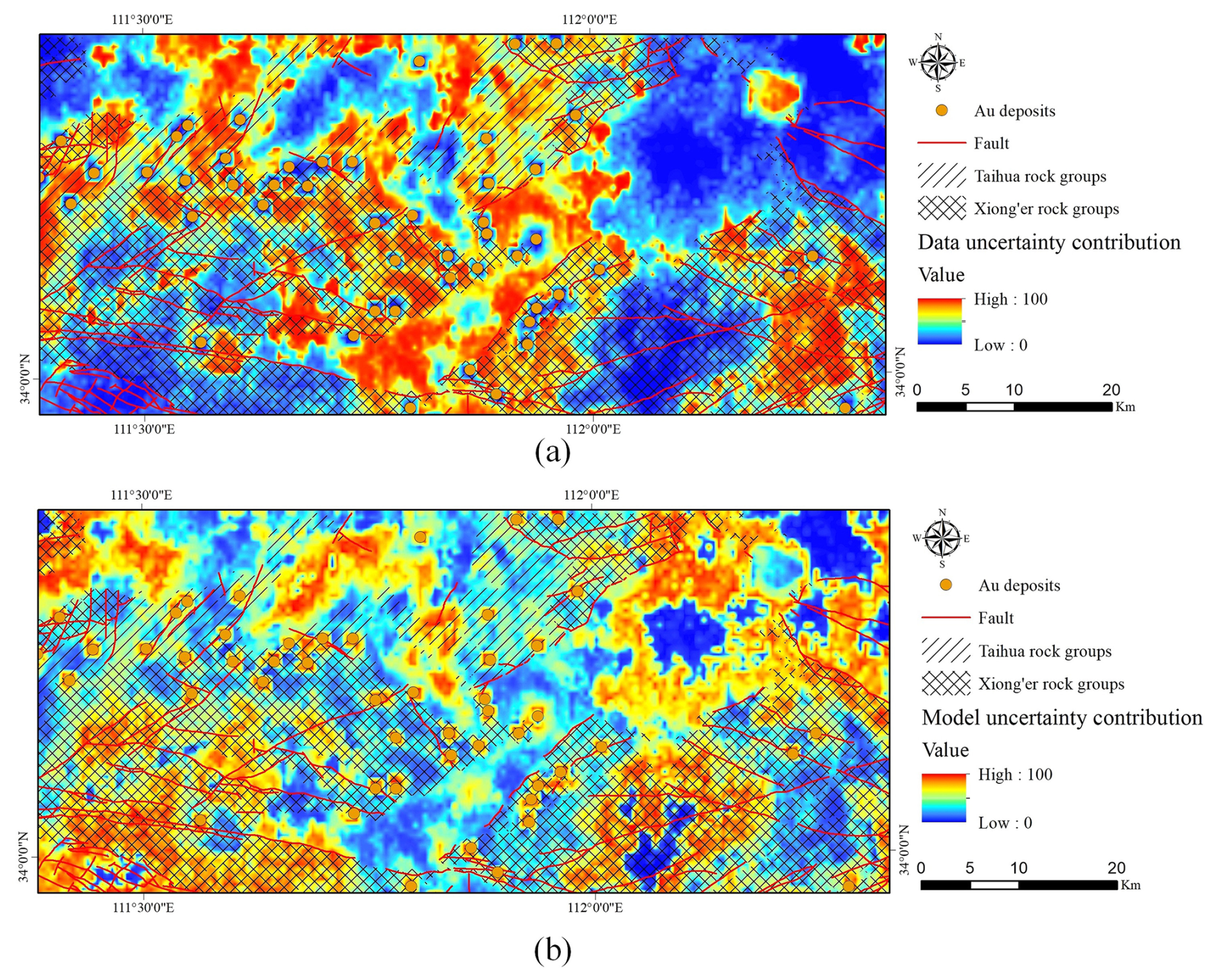
To quantify the relative contribution of data and model uncertainties to the total predictive uncertainty in MPM, a dominant uncertainty map is presented using the variance decomposition (Grömping, 2007). This statistical approach enables the partitioning of total predictive variance into components attributable to data variability and model stochasticity, thereby providing a clearer understanding of uncertainty sources and supporting more informed exploration decisions. The data uncertainty (Var_data) exhibits geologically meaningful patterns, reflecting the influence of heterogeneous simulated evidence layers. In contrast, the model uncertainty (Var_model) primarily captures limitations of the network architecture and parameters, highlighting areas where CNN struggles to generalize. Then, the relative contribution of each component can be calculated as their ratio to the total predictive uncertainty (Var_total).

Compared with the uncertainty maps in Figs. 12 and 13, the uncertainty decomposition maps (Fig. 15) identify the dominant source of predictive uncertainty rather than its magnitude at each location. Obviously, high data uncertainty contribution (Fig. 15a) exhibits broader spatial influence, whereas high model uncertainty contribution (Fig. 15b) is more localized with lower magnitude. This finding suggests that variability in the evidence layers is the primary source of total uncertainty. Moreover, the clustering of data uncertainty around known mineral deposits further reflects its dominant contribution to total uncertainty. Such decomposition provides additional diagnostic information beyond individual uncertainty maps and helps identify whether future efforts should focus on improving input data quality or model development. Consequently, enhancing the quality and representativeness of input evidence layers is likely to be more effective in reducing total MPM uncertainty than solely optimizing CNN architecture or parameters.

Figure 15 Uncertainty contribution maps: (a) data uncertainty, (b) model uncertainty.

7.2 Relationship between predictive probability and uncertainty

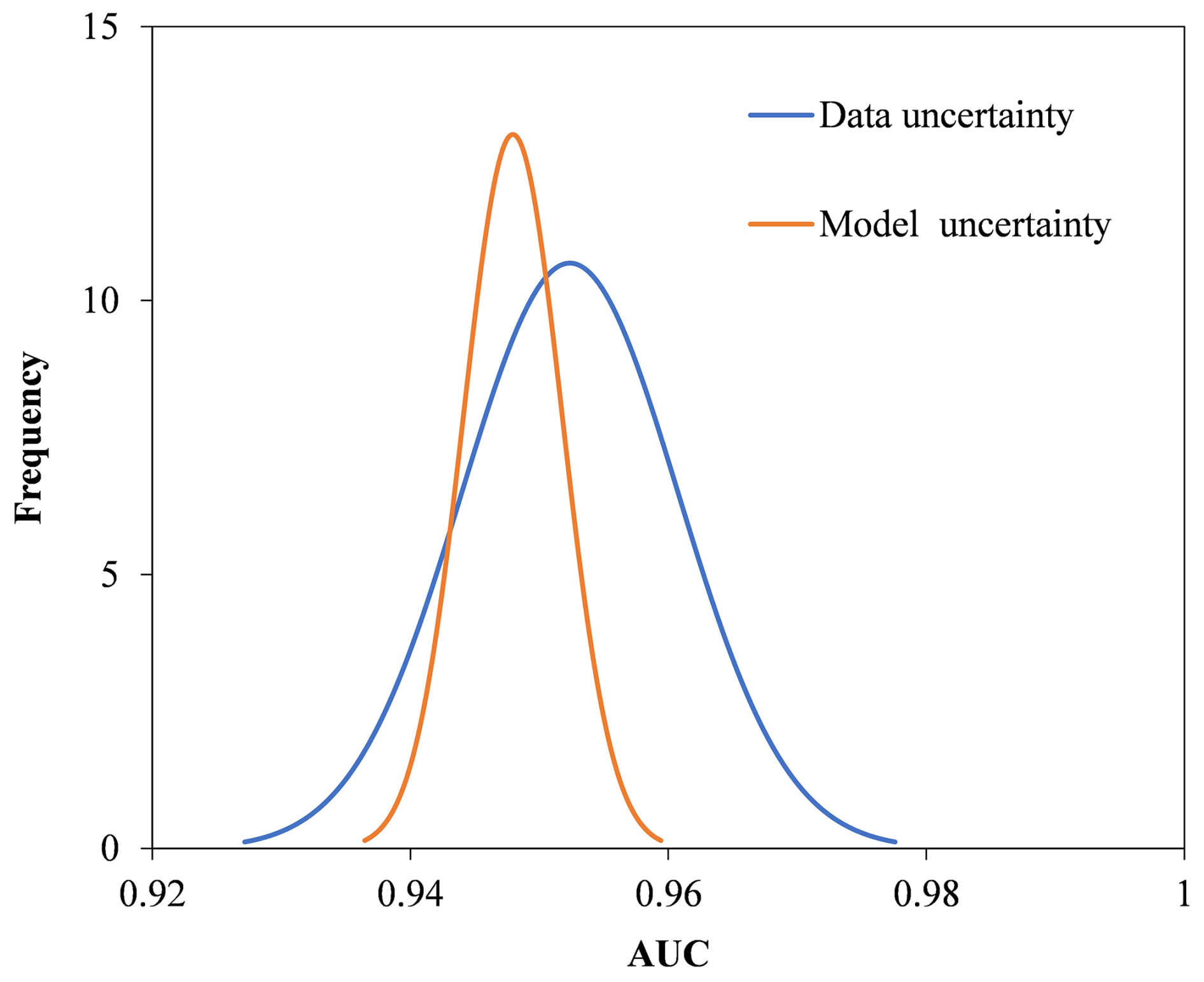
To investigate the relationship between predictive probability and uncertainty, the mean predictive probability and uncertainty were jointly analyzed using a pixel-wise scatter plot. The mean-uncertainty scatter plots (Fig. 16) show the relationship between the mean predictive probability and predictive uncertainty in the study area, providing a direct visualization of how data uncertainty and model uncertainty vary with the mean predictive values. In this inverted U-shaped distribution plot, each scatter point represents one pixel of the study area, with the x-axis indicating the mean predictive probability obtained from multiple stochastic forward passes and the y-axis representing the corresponding entropy value. Data uncertainty exhibits a generally greater magnitude than model uncertainty, indicating that variability in the geological evidence layers contributes more to the predictive uncertainty than instability in the model's architecture and parameters. The area under the receiver operating characteristic curve (AUC) (Hanley and McNeil, 1982) is another robust metric widely adopted to quantitatively measure model performance, particularly in the presence of class imbalance. Figure 17 presents the frequency distribution of AUC values derived from 100 realizations for data uncertainty and model uncertainty. Both distributions are centered around AUC ≈ 0.95, indicating that CNN model maintains consistently high predictive accuracy across multiple simulations. However, the wider spread of the data uncertainty curve reflects greater variability in predictive performance due to fluctuations in the evidence layers. In contrast, the narrower spread of the model uncertainty curve demonstrates that the models' architecture and parameters remain relatively stable during stochastic forward passes. Such results further emphasize the importance of optimizing mineral deposit models and weighting strategy by identifying the most influential geological features, as they exert more influence on predictive uncertainty.

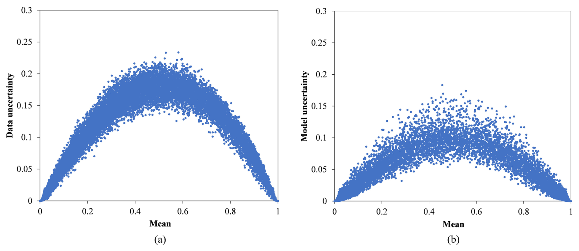
Figure 16 Scatter plots of mean probability versus uncertainty: (a) data uncertainty, (b) model uncertainty. The x-axis denotes the mean predictive probability obtained from multiple stochastic forward passes and the y-axis denotes the corresponding uncertainty (entropy).

Figure 17 Frequency distribution of AUC values: (a) data uncertainty, (b) model uncertainty.

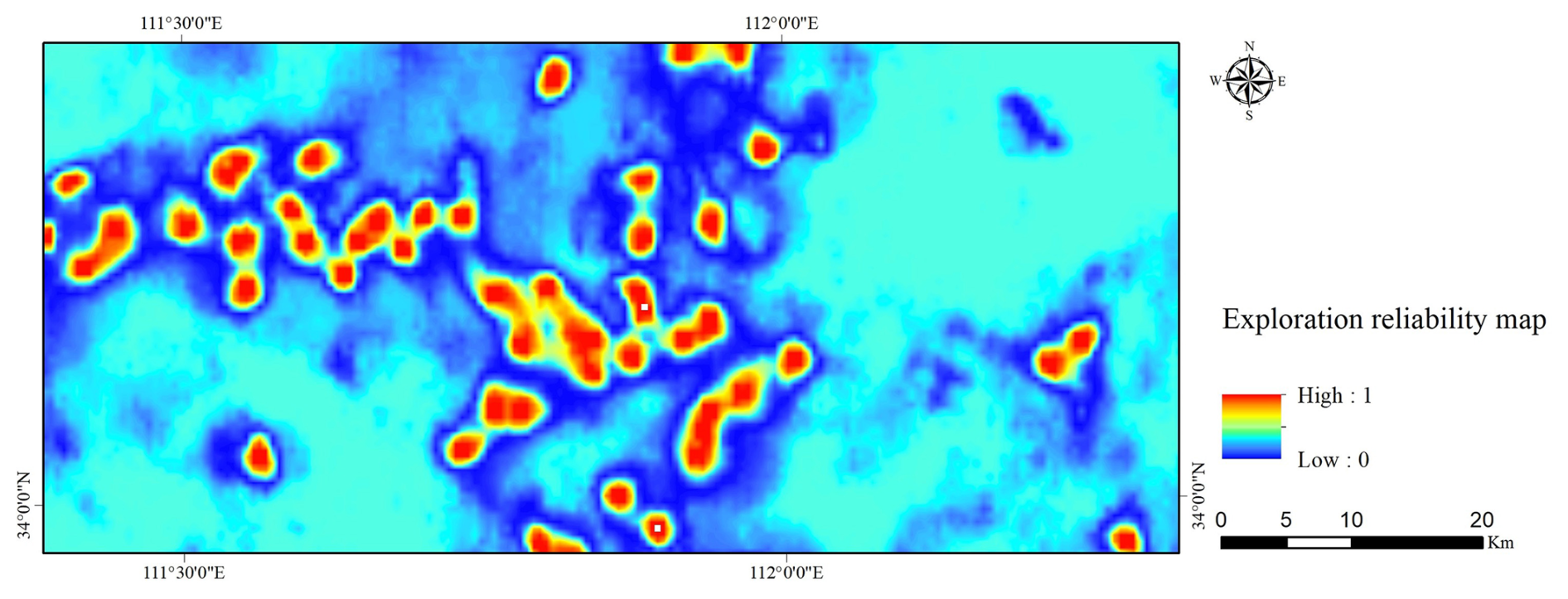
To further facilitate the exploration target prioritization, an exploration reliability map (Fig. 18) is delineated by integrating both the mean predictive probability with predictive uncertainty:

$$\begin{array}{}\text{(8)}& R\left(p\right)={\stackrel{\mathrm{‾}}{p}}^{*}-H(p{)}^{*},\end{array}$$

where ${\stackrel{\mathrm{‾}}{p}}^{*}$ and H(p)^* denote the normalized mean predictive prospectivity and normalized predictive entropy, respectively. This normalization places both variables on the same scale, allowing predictive potential and reliability to be considered simultaneously. Areas with high values represent locations correspond to both high prospectivity and low uncertainty, and are therefore regarded as the most reliable exploration targets. Compared with the mean prospectivity map alone, this map suppresses regions with high uncertainty while preserving areas with consistently high prospectivity, thereby providing a more reliable basis for exploration decision-making.

Figure 18 The exploration reliability map.

7.3 Geological significance

Uncertainty quantification provides essential insights into the reliability of MPM. On the one hand, it delineates regions characterized by low uncertainty and high prospective probability, thereby guiding exploration efforts toward areas with the greatest potential of new mineral discoveries. On the other hand, it facilitates the interpretation of spatial relationships between mineral prospectivity and major geological features. By decomposing total uncertainty into data uncertainty and model uncertainty, the proposed framework establishes a quantitative basis for evaluating the credibility of predictive outcomes. Such differentiation enables the identification of whether uncertainty stems from inappropriate evidence layers or model limitations. Specifically, regions with high prospectivity and low uncertainty represent high-confidence exploration targets, whereas high uncertainty areas correspond to high-risk but potential opportunities. Consequently, uncertainty quantification not only enhances the interpretability of MPM but also supports informed decision-making in mineral exploration.

7.4 Future prospects

Future advances in uncertainty quantification for MPM are expected to focus on improvements in data quality, modeling strategies, interpretability, and decision optimization to reduce predictive uncertainty. From a data perspective, enhancing the geological representativeness of evidence layers and developing more reliable strategies for negative sample selection are critical for reducing data uncertainty and more accurately capturing the spatial variability of mineralization controls. Regarding the uncertainty modeling, progress should extend beyond conventional Monte Carlo dropout toward Bayesian inference and ensemble learning capable of jointly characterizing both data and model uncertainties. In terms of the uncertainty interpretability and visualization, embedding geological knowledge directly into deep learning architectures and loss functions offers a promising way to constrain model training, reduce high-uncertainty output, and enhance the transparency of predictions (Zuo et al., 2023, 2024). In addition, feature attribution is also valuable for identifying which evidential layers drive most to high prospectivity or high uncertainty, thereby strengthening geological interpretability (Dwivedi et al., 2023). Finally, integrating uncertainty quantification with risk-return analysis will support the selection of exploration targets that balance mineralization potential against geological risk, translating probabilistic predictions into more actionable decision support (Wang et al., 2020).

8 Conclusions

This study proposes an integrated framework for uncertainty quantification in deep learning-based MPM. The framework quantifies data uncertainty, model uncertainty, total predictive uncertainty, and is illustrated through a case study of gold prospectivity mapping in western Henan Province of China. Uncertainty quantification transforms MPM from a purely predictive approach into a decision-support framework, enabling more valuable mineral exploration.

1. Data uncertainty in MPM arises from subjective interpretation of geological feature modeling, as well as relatively limited spatial resolution of geochemical and geophysical data, which is modeled through stochastic simulation of evidence layers constrained by geological understanding. Model uncertainty reflects variability in network architecture and parameter estimation, which is modeled using a Bayesian CNN with Monte Carlo dropout.

2. Contribution analysis reveals that data uncertainty is the dominant source of total predictive uncertainty in MPM, exhibiting more geologically meaningful patterns than model uncertainty. This finding indicates that improving the quality and representativeness of evidence layers is more effective for reducing overall uncertainty than optimizing CNN architecture and parameters.

3. Uncertainty quantification enhances the reliability of MPM by distinguishing between data- and model-driven uncertainties. Areas characterized by high prospectivity and low uncertainty represent robust exploration targets, while those with high uncertainty highlight regions requiring improved geological knowledge or further model refinement.