Multi-season evaluation of temperature and wind in the marine boundary layer along the United States northeast coast in the High-Resolution Rapid Refresh model

The High-Resolution Rapid Refresh (HRRR) model is run operationally by the National Oceanic and Atmospheric Administration to provide high-resolution short-range forecasts for the continental United States. The evaluation of the HRRR model off of the United States coasts has been challenged by the lack of suitable continuous profile observations in the marine boundary layer in the past. State-of-the art remote sensing instruments were recently deployed along the coast of New England in the northeastern United States for the multi-year Third Wind Forecast Improvement Project and provide a unique opportunity for the evaluation of temperature and wind in the marine boundary layer in the HRRR model. We used 1 year of data at three sites, two of which were on islands, to document the seasonal characteristics of the marine boundary layer and its representation in the HRRR model for different forecast hours. Overall, the HRRR model captured the seasonal and diurnal evolution of temperature and wind very well. However, low-level horizontal wind shear and static stability were too weak in the model, especially during the warmer months. At certain sites, these biases were accompanied by errors in sea surface temperature, suggesting a potential, though localized, link. Low-level jets (LLJs) occurred in approximately 20 % of the hourly profiles with a maximum frequency during spring and summer. Up to 60 % of the LLJ profiles during peak seasons were correctly predicted, using the critical success index as a measure. Systematic model errors in wind and temperature were found during LLJs, when the HRRR model frequently underestimated wind speed at nose height and shear below nose height, often accompanied by static stability that was too weak. These errors resulted in low-level Bulk Richardson numbers that were consistently too large at all three sites, indicating an overestimation of dynamic stability in the boundary layer in the model. Such systematic errors in low-level wind shear and stability were largely absent during correct rejections, that is, when an LLJ was neither observed nor simulated, indicating that LLJs were responsible for a large part of the model errors.

1 Introduction

The High-Resolution Rapid Refresh (HRRR) model is a numerical weather prediction (NWP) model that is run operationally every hour at the National Oceanic and Atmospheric Administration (NOAA) National Centers for Environmental Prediction providing high-resolution, short-range (0–18 h) forecasts for the continental United States, with forecasts out to 48 h when the model is initialized at 00:00, 06:00, 12:00, and 18:00 UTC (Dowell et al., 2022; James et al., 2022). It provides guidance for rapidly evolving mesoscale weather phenomena, such as convective storms, downslope windstorms, fog and low cloud ceilings, cold fronts, smoke plumes from active wildfires, and rapid changes in wind and solar energy sources. Numerous studies evaluated the HRRR model for specific atmospheric phenomena, such as convective storms (e.g., Duda and Turner, 2021), cold air pools and flows in mountainous terrain (e.g., Olson et al., 2019; Adler et al., 2023a, b), boundary layer height structure and evolution (e.g., Fovell and Gallagher, 2020; Bianco et al., 2026), and surface fluxes (e.g., Lee et al., 2019). A more detailed overview of recent HRRR evaluation studies is given in Table 1 in James et al. (2022). Almost all HRRR evaluation studies focused on phenomena that occur over land in the terrestrial atmospheric boundary layer. Fewer studies have investigated the performance of the HRRR in the marine boundary layer along the United States east coast (e.g., Djalalova et al., 2016; Pichugina et al., 2017; James et al., 2018; Myers et al., 2024; Naegele et al., 2025) and west coast (e.g., Liu et al., 2025). Most of them focused on low-level wind due to the relevance of accurate wind forecasts for offshore renewable energy.

Precise HRRR model forecasts of the marine boundary layer have a direct benefit for many sectors of society due to their relevance for fisheries, aviation safety, offshore energy production, recreation, tourism, and search and rescue. The coastal environment presents a challenge for NWP models because of complex topography, sharp gradients in surface roughness and temperature, and the interaction between waves and winds whose coupling is usually not considered in NWP (e.g., Shaw et al., 2022). In addition, the large decrease in the density of observations offshore is problematic for model data initialization (e.g., Djalalova et al., 2016). One atmospheric phenomenon that is potentially challenging to forecast correctly by NWP models is the coastal low-level jet (LLJ). LLJs are characterized by a pronounced wind speed maximum in the lowest few hundred meters of the atmosphere. Models often overestimate nose height and underestimate nose height wind speed (e.g., Li et al., 2021; Quint et al., 2025). Along the United States east coast, wind directions in the LLJs are often southwesterly and form from horizontal temperature gradients between the land and ocean surface and may be intensified by frictional decoupling under stable stratification or frontal passages (e.g., Debnath et al., 2021; De Jong et al., 2024). Using 9 years of anemometer data collected on an offshore light station and a buoy in the New York Bight, Colle and Novak (2010) reported a clear seasonality of LLJ occurrence with maxima in spring and summer when the land-sea surface temperature differences are large, and a pronounced diurnal cycle with LLJs occurring mostly in the late afternoon until the early morning hours. Sea-breeze circulations in the New York Bight are frequently associated with LLJs, especially from late spring through fall, which was investigated by McCabe and Freedman (2023, 2025) using coastal and buoy-based lidars and surface stations and modeling sensitivity studies. The inland propagation of the sea breeze and the LLJ intensity are found to be sensitive to cold water upwelling (McCabe and Freedman, 2026). Numerical studies suggest that LLJs are spatially extensive along the United States east coast and occur particularly frequently near the state of Massachusetts (Aird et al., 2022; Quint et al., 2025).

The evaluation of NWP models in the marine environment is challenged by the lack of suitable observations (e.g., Shaw et al., 2022). Most long-term observations offshore have been made near the surface from buoys, which are sparsely deployed. In recent years, buoy-mounted lidar systems have provided long-term observations of horizontal wind and turbulence profiles, but these buoys are even more sparse and measurements are mostly limited to altitudes below 200 m. No long-term observations of temperature profiles with high temporal frequency are currently available in the marine boundary layer in this region. To identify model errors in the marine boundary layer and to improve the operational forecasts at the coastal regions, in-depth process-level model evaluations are needed. The success of this approach was, for example, demonstrated during the Second Wind Forecast Improvement Project (Shaw et al., 2019) where observationalists from the public and private sector and model developers at NOAA worked together to improve the HRRR forecasts in the complex mountainous terrain of the Columbia River Basin in the Pacific Northwest (e.g., Olson et al., 2019; Wilczak et al., 2019; Banta et al., 2021; Bianco et al., 2022; Adler et al., 2023b).

Comprehensive observations in the marine boundary layer along the coast of New England were recently collected in the framework of the Third Wind Forecast Improvement Project (WFIP3,  Kirincich et al., 2026), which provide a unique opportunity for the evaluation of the HRRR model in the marine environment. The field campaign period spanned more than one year, from February 2024 to August 2025, allowing for the investigation of seasonal patterns in the model errors. A barge was deployed for a limited period of a few months in summer 2024, allowing the investigation of wind and temperature structure in the undisturbed marine boundary layer (Bodini et al., 2026). In this study, data from three land-based sites were analyzed for a 12-month period, with two sites located on islands off the southern New England coast and one located near the coastline of the mainland. State-of-the-art ground-based remote sensing instruments for temperature and wind profiling throughout the whole depth of the marine boundary layer were deployed at each of the sites. The aims of this study are to document the observed seasonal and diurnal cycle of temperature and wind in the marine boundary layer and to use these observations to evaluate the accuracy of the HRRR model for different forecast hours. Special attention is given to LLJs, since those are found to be associated with systematic model errors.

2 Investigation area, data, and methods

The investigation area is located in the northeastern United States along the coast of southern New England. We used data from three WFIP3 sites (locations in Fig. 1a, b) and investigated the period March 2024 through February 2025, which was chosen based on data availability for the sites. Two sites were located on islands, namely, NANT on Nantucket Island and BLOC on Block Island. The third site, RHOD, was located on the southeastern coast of Rhode Island. Due to the location of the sites on land, the local boundary layer conditions do not represent the pure maritime boundary layer but are impacted by an internal boundary layer forming from the influence of the land. This impact is likely the smallest at NANT for southerly flow because of the site location within a few hundred meters of the southern coastline of Nantucket Island (Fig. 1c, d), and we expect model errors at this site to most closely resemble those in the maritime boundary layer. BLOC is located at the local airport in the interior of Block Island, around 2 km away from the ocean and around 35 m above mean sea level (Fig. 1e). Since Block Island has only five land grid points in the HRRR model due to its 3 km horizontal grid spacing (Fig. 1f), the terrain features and site locations are not correctly represented. Hence, we expect model errors close to the ground at this site, although above the internal boundary layer the basic characteristics of the marine boundary layer should still be well represented.

Figure 1 Terrain height based on (a) 30 m resolution elevation data from the Shuttle Radar Topography Mission (SRTM) and (b) terrain height from the 3 km HRRR model output in the northeastern United States. The location of the investigation area relative to the continental United States is indicated by the red box in the map inset. The station locations at Block Island (BLOC), Rhode Island (RHOD), and Nantucket Island (NANT); the locations of the buoys (Buoyz01 and Buoy44085); the states of New York (NY), Connecticut (CT), Rhode Island (RI), and Massachusetts (MA); and the location of Long Island are also indicated. The SRTM (left) and model terrain (right) are shown for (c, d) Nantucket Island, (e, f) Block Island, and (g, h) Rhode Island. Gray contour lines show state boundaries and coastlines from Natural Earth Data (https://www.naturalearthdata.com, last access: 7 January 2026).

These three sites were chosen from all sites deployed for WFIP3 because a very similar set of remote sensing instruments was operated at each of the sites to observe temperature and wind profiles throughout the boundary layer. These include radar wind profilers and multiple Doppler lidars for wind and an infrared spectrometer (IRS) for temperature. Ceilometers provide information on cloud base height.

To combine the different instruments for wind and to retrieve temperature from the passive IRS, we used two optimal estimation retrievals. For temperature profiles, we used the optimal estimation physical retrieval TROPoe (Turner and Löhnert, 2014; Turner and Blumberg, 2019; Turner and Löhnert, 2021; Adler et al., 2024; Letizia et al., 2025) that has been used for boundary layer studies for more than 10 years. For wind profiles, we used the optimal estimation retrieval WINDoe (Gebauer and Bell, 2024). WINDoe was developed fairly recently following the same concept as TROPoe. Software for both retrievals are freely available online (see “Code and data availability” section).

In the following sections, we describe the individual observational data sets, the processing of the observational data with TROPoe and WINDoe, the HRRR model data, and the methods used for model evaluation and LLJ detection.

2.1 Observational data

This section gives a brief overview of the observational data sets. Additional information can be found in Sects. S1 and S2 in the Supplement and the metadata of the uploaded data sets (see “Code and data availability” section).

2.1.1 Radar wind profiler

Radar wind profilers are active ground-based remote sensing instruments that emit a pulsed electromagnetic signal, here at 915 MHz, which is intercepted and backscattered by refractive index fluctuations (e.g., Ecklund et al., 1988). Profiles of horizontal wind components are obtained from the first moment of the Doppler spectra in two modes, high and low vertical resolution. The modes differ in vertical measurement range and resolution; the high-resolution mode has a higher vertical resolution but lower maximum range. The profilers at NANT and BLOC provided profiles every 15 min using 30 min overlapping averaging windows. The profiler at RHOD provided hourly averaged profiles. While the wind profiles from radar wind profilers have a lower vertical resolution and higher lowest measurement range gate than those obtained from Doppler lidars, radar wind profilers have the great advantage of being able to measure through clouds, during precipitation, and higher up in the atmosphere where the signal-to-noise ratio of Doppler lidars is usually insufficient.

2.1.2 Doppler lidar

Doppler lidars are active remote sensing instruments that emit laser pulses, here at 1.5 µm, and measure the Doppler shift of the backscattered energy. In contrast to radar wind profilers, aerosols in the atmosphere are the main scatterers. Two types of lidars are used in this study, which we refer to as profiling and scanning lidars. The profiling lidars are low-pulse energy systems that profile the lowest several hundred meters of the atmosphere. The manufacturer software provided 10 min (NANT and RHOD) and 2 min (BLOC) averaged profiles of the horizontal wind components between 50 and 200 m at NANT and BLOC and between 10 and 280 m at RHOD. From the higher-powered scanning lidars we used radial velocity measurements at an elevation angle of 60° at six different azimuth angles with a resolution of approximately 30 m along the line of sight and the lowest usable range gate at approximately 70 m. The vertical range of these scanning lidars usually spans the boundary layer and is limited by aerosol availability and the presence of clouds and fog in the line of sight.

2.1.3 Surface tower

At each site, near-surface in situ temperature, humidity, wind, and pressure were measured with a tower. Temperature was measured at 2 m a.g.l. (m above ground level) at all three sites, whereas wind was measured at 10 m a.g.l. at BLOC and at 4 m a.g.l. at NANT and RHOD.

2.1.4 Infrared spectrometer

The deployed ground-based IRS were Atmospheric Sounder Spectrometer by Infrared Spectral Technology (ASSIST, Michaud-Belleau et al., 2025). These instruments are passive spectrometers that receive spectrally resolved downwelling infrared radiation between the wavelengths of 3 and 19 µm (525–3300 cm⁻¹) with a temporal resolution of approximately 15 s. The ASSIST is very similar to the Atmospheric Emitted Radiance Interferometer (AERI, Knuteson et al., 2004a, b). The instruments have a hatch that closes during precipitation to protect the fore optics, which inhibits measurements during rain or snow.

2.1.5 Ceilometer

Ceilometers are active remote sensing instruments that provide attenuated backscatter profiles from which cloud-base height is derived using the manufacturer's algorithm with a temporal resolution of approximately 16 s. The lowest cloud base height detectable by the instruments in this study is about 40 m.

2.1.6 Operational Sea Surface Temperature and Ice Analysis (OSTIA)

Sea surface temperature (SST) was obtained from the Operational Sea Surface Temperature and Ice Analysis (OSTIA), which combines satellite and in situ observations. The data set provides a daily analysis of SST with a spatial resolution of approximately 6 km (Good et al., 2020). The OSTIA products are continuously monitored and validated, have been found to have near zero biases, and are routinely used as boundary conditions for operational NWP models in Europe (Donlon et al., 2012). To assess the accuracy of OSTIA in the investigation area, we compared OSTIA SST with in-situ near-surface water temperature measurements at two buoys (locations in Fig. 1a). The agreement was very good (Fig. S2 in the Supplement) with the absolute value of the mean bias smaller than 0.04 °C. This is consistent with McCabe and Freedman (2026) who reported good agreement between daily OSTIA SST and buoy-based measurements in the New York Bight, just south of the WFIP3 investigation area. OSTIA and buoy data revealed a clear spatial difference in SST between the two locations. During the summer months, the buoy that was located further north (Buoy44085) was several degrees colder than the buoy further south (Buoyz01). Inspection of OSTIA SST spatial fields revealed the presence of a cold tongue extending into the northern part of the investigation area from the east.

Given the very good agreement of OSTIA SST with in situ measurements, we consider the OSTIA SST the truth and used it to evaluate the SST in the HRRR model in the vicinity of the three measurement sites. Daily values at the grid points closest to the sites were extracted and linearly interpolated to match the hourly time stamp of the model.

2.2 Retrieval of temperature and wind profiles

2.2.1 TROPoe

Thermodynamic profiles and liquid water path (LWP) were retrieved every 10 min from the instantaneous infrared radiances measured by the IRS using the optimal estimation physical retrieval TROPoe (Turner and Löhnert, 2014; Turner and Blumberg, 2019; Turner and Löhnert, 2021; Adler et al., 2024). In addition to infrared radiances, input data in TROPoe included the cloud‐base height from a collocated ceilometer (NANT and BLOC) or Doppler lidar (RHOD) and the temperature, water vapor mixing ratio, and air pressure from in situ near‐surface observations. In addition to this temporally resolved input data, the retrieval requires climatological priors of temperature and humidity, which we computed from operational radiosondes launched at Upton, New York. The retrieval produces an estimate of temperature and water vapor profiles with 55 vertical levels each from the surface up to 17 km as well as LWP. The distance between levels starts at 10 m and increases with height. Starting with the prior as a first guess, a forward model is used to compute pseudo-observations, which are then compared to the actual observations. If the computed and observed values do not agree within the uncertainty of the measurements, the state vector is modified in an iterative process. For example, Blumberg et al. (2015) and Bianco et al. (2024) evaluated such retrieved profiles against radio soundings and found a good agreement in the atmospheric boundary layer. These results were also corroborated by comparisons with a 135 m met tower from Letizia et al. (2026), who demonstrated biases less than 0.3 K at multiple heights.

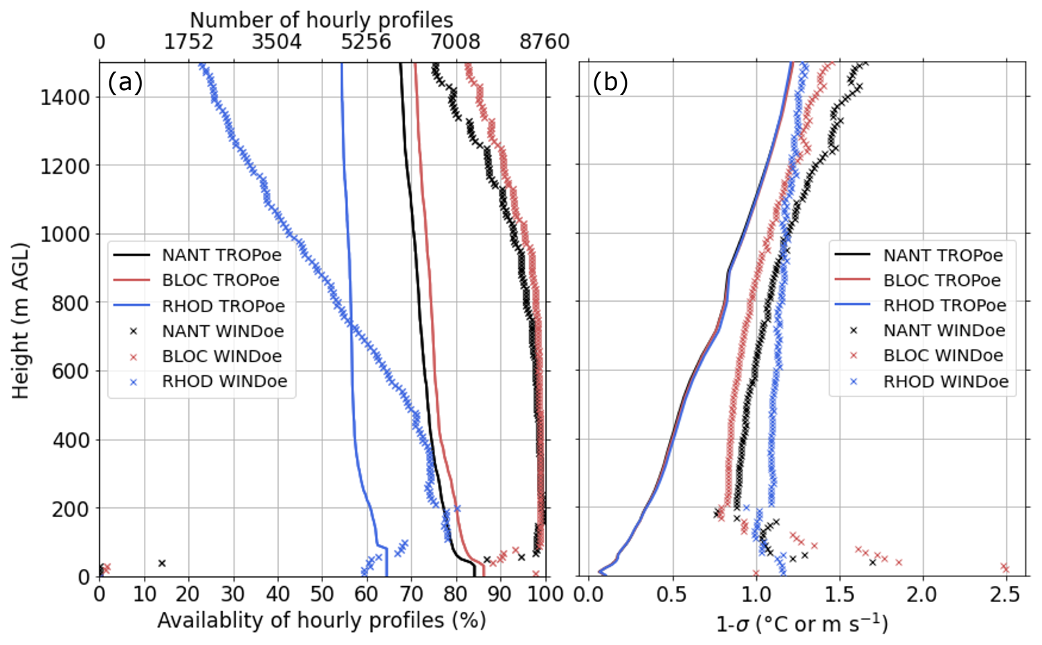
Figure 2 Profiles of (a) availability and (b) mean 1σ uncertainty of hourly temperature and wind observations at NANT, BLOC, and RHOD retrieved with TROPoe and WINDoe. The 1σ uncertainties for the three TROPoe retrievals in (b) are essentially identical and thus overlap. In (a), missing data are related to power outages and hardware and software issues. In addition, the availability of temperature profiles is limited by clouds that are opaque in the infrared, and the availability of wind profiles is limited by the range of the individual instruments used in WINDoe.

TROPoe provides a number of output variables that allow one to distinguish between solutions with good and dubious quality. In this study, we used the same criteria as described in Adler et al. (2024). IRS-based retrievals have little to no information content above cloud base depending on the optical depth of the cloud (Turner, 2007). This makes observed cloud base height a very important input variable to inform TROPoe where the lowest cloud base height is located. If the infrared radiance observations indicated the presence of liquid water in the profile using a threshold of LWP > 8 g m⁻², but no cloud base height was observed, we did not use this profile in our analysis. The threshold value was determined empirically and found to work well for a variety of locations and conditions (Adler et al., 2024). If a cloud base height was detected and LWP > 8 g m⁻², we only used data below cloud base height. After filtering for quality and clouds, we computed hourly averaged profiles centered on the hour from the 10 min retrievals. This resulted in a data availability of around 85 % at the surface at NANT and BLOC and around 65 % at RHOD during the 1-year period (Fig. 2a). In approximately 10 % of these profiles, cloud base height was below 300 m, explaining the sharp reduction in availability with height in the lowest few hundred meters.

The TROPoe retrieval propagates the observational uncertainty and allows the computation of the 1σ uncertainty profiles of temperature as the square root of the diagonal elements of the posterior covariance matrix. The uncertainty is very small near the surface and increases with height to around 1.2 K at 1500 m, which is very consistent for the three sites (Fig. 2b).

2.2.2 WINDoe

With the high- and low-resolution modes of the radar wind profilers, the two Doppler lidars, and the tower, we have five different data sets with information on horizontal wind at each site that have very different vertical and temporal resolution, and each is associated with specific uncertainties. The WINDoe retrieval (Gebauer and Bell, 2024) allows combining the individual data sets and outputs into one profile, taking into account the information and uncertainties of each data set. The use of WINDoe minimizes data gaps and maximizes data availability, compared to using wind profiles from only one of the instruments. WINDoe follows the same optimal estimation concept as TROPoe (Sect. 2.2.1). In this study, we used hourly retrieved wind profiles considering data from each input source in a 30 min window, except for the radar wind profiler at RHOD, which was available for 60 min averaging periods. The wind retrievals were computed for an equidistant height grid with 10 m spacing, which makes it very easy to compare to model output.

Like TROPoe, WINDoe requires climatological information on horizontal wind components as a first guess. Because of the larger number of vertical levels (376 levels for each of the u- and v-components), the number of operational radiosondes at Upton, New York, was not sufficient to obtain good level-to-level covariances for monthly priors. As a rule of thumb, the number of profiles should be at least 1 order of magnitude larger than the state vector (752 in our case). This means that even a decade of twice-daily radiosonde profiles would only provide the same order of magnitude for each monthly prior. Instead we used hourly HRRR profiles at initialization time from three grid points distributed through the WFIP3 area spanning multiple years, which allowed us to compute monthly priors from more than 11 000 profiles per month. Due to the high information content of the active remote sensing instruments used as input to WINDoe and the 1σ uncertainty of the u- and v-components of the prior being 1 order of magnitude larger than the observation uncertainty, the prior has a negligible impact on the retrieved profiles when and where observations are available, allowing us to use the retrieved profiles for the evaluation of the HRRR model. We use the 1σ uncertainty for the wind components σ_u, σ_v computed as the square root of the diagonal elements of the posterior covariance matrix to filter retrieved values where little to no information was available from any of the input data sets by requiring both σ_u and σ_v to be less than the empirically determined threshold of 2.5 m s⁻¹.

Data availability of the retrieved wind profiles after filtering is close to 100 % at NANT and BLOC in the lowest few hundred meters and is still higher than 75 % at 1500 m (Fig. 2a). At RHOD, availability in the lowest 400 m is around 75 % and drops to only 20 % at 1500 m, related to an overall lower availability of the individual input measurements.

From σ_u, σ_v we estimated the 1σ uncertainty of horizontal wind speed assuming that the u- and v-components are uncorrelated (Archer, 2025):

$$\begin{array}{}\text{(1)}& {\mathit{\sigma }}_U\approx \sqrt{{\left({\displaystyle \frac{u}{U}}\right)}^{\mathrm{2}}\cdot {\mathit{\sigma }}_u^{\mathrm{2}}+{\left({\displaystyle \frac{v}{U}}\right)}^{\mathrm{2}}\cdot {\mathit{\sigma }}_v^{\mathrm{2}}}\end{array}$$

with U being the horizontal wind speed. The average 1σ uncertainty of wind speed was approximately between 0.8 and 1.5 m s⁻¹ in the lowest 1.5 km at all sites (Fig. 2b). Values increased towards the surface, especially at NANT and BLOC, which was owed to the gap in input data between around 50 m (lowest height of the profiling lidar) and the surface tower (Fig. 2a).

Since WINDoe has not been as widely used for research as TROPoe, we compared the retrieved wind speed profiles to the profiles of the individual instruments that were used as input to assess if there were any major differences (Sect. S2). The differences between the retrieved wind speed and the wind speed from the individual inputs are well within the uncertainty of the retrieval.

2.3 High-Resolution Rapid Refresh (HRRR) model

We evaluated the operational version of NOAA's HRRR model (version 4,  Dowell et al., 2022; James et al., 2022) that has been operational since December 2020. The operational HRRR model is run hourly with an independent initial condition created by the HRRR Data Assimilation System (HRRRDAS) (Dowell et al., 2022) which leverages the Rapid Refresh model (Benjamin et al., 2016) analyses twice daily as a background for data assimilation to constrain the synoptic scale evolution. The HRRR provides 18 h forecasts, but every 6 h, at 00:00, 06:00, 12:00, and 18:00 UTC, the forecast horizon is extended to 48 h. The HRRR assimilates a broad set of observations, including data from radiosondes, radars, aircraft, surface stations, buoys, and satellites. No measurements from the WFIP3 campaign that are used for the model evaluation in this study were assimilated. HRRR version 4 uses the Mellor-Yamada-Nakanishi-Niino eddy-diffusivity mass-flux (MYNN-EDMF) scheme for the planetary boundary and surface layer and subgrid-scale clouds, the Rapid Update Cycle land surface model (RUC LSM) for the land surface, the Rapid Radiative Transfer Model for general circulation models (RRTMG) for radiation, and the Thompson aerosol-aware scheme for cloud microphysics (details in Dowell et al., 2022).

The first model level is just below 10 m, and vertical grid spacing increases from about 25 m near the surface to 300 m at 1.5 km with a total of 10 levels below 1.5 km. The horizontal grid spacing is 3 km, and we selected the grid point that is closest to the location of each site and over land for comparison to the observed profiles (Fig. 1d, f, h). In this study, we concatenated hourly model output for each forecast horizon starting at 0 (initialization time) out to 18. This resulted in a continuous time series for each forecast horizon that could be compared to the observations.

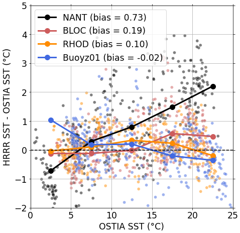
Figure 3 Difference in daily SST (HRRR model minus OSTIA) over OSTIA SST at grid points that are just off the coasts of NANT and BLOC and at the Buoyz01 location. HRRR data at initialization time are shown. The hourly HRRR SST was averaged to daily values. The solid lines indicate mean values averaged over bins of 5° width.

SST in the HRRR model comes from the Global Data Assimilation System (GDAS) operated by the NOAA National Centers for Environmental Prediction. We compared daily averaged HRRR SST to OSTIA SST at four locations (close to NANT, BLOC, RHOD, and Buoyz01) and found differences depending on location and season (Fig. 3). When SST was cool (less than 15 °C), the HRRR SST and OSTIA SST agreed relatively well at all locations on the average (mean difference <1 °C). When SST exceeded 15 °C, which was approximately the case between June and November (Fig. S2), SST in the HRRR was frequently overestimated by several degrees at NANT, while it was slightly underestimated at RHOD and Buoyz01 on the average. McCabe and Freedman (2025) found that the bias in SST between HRRR and OSTIA varied spatially in the New York Bight during summer sea-breeze events with a warm bias near the coasts and a cold bias further offshore possibly owing to coastal upwelling.

2.4 Low-level jet criteria and evaluation metrics

To detect LLJs in the observed and simulated hourly wind profiles, we used criteria based on maximum wind speed and wind speed decrease above the nose, which were first developed by Bonner (1968) and which has also been applied in previous studies on coastal LLJs in the area (e.g., Quint et al., 2025; Bodini et al., 2026). Other studies used a less restrictive method to detect LLJs in the area, e.g., McCabe and Freedman (2023, 2025) who defined the LLJ as a wind speed maximum between 150 and 300 m. As pointed out by Hallgren et al. (2023), there is no consensus regarding how LLJs should be defined and the choice of criteria a as well as the vertical window from which the LLJs are extracted impact the LLJ frequency and morphology. Hence care should be taken when making cross-study comparisons.

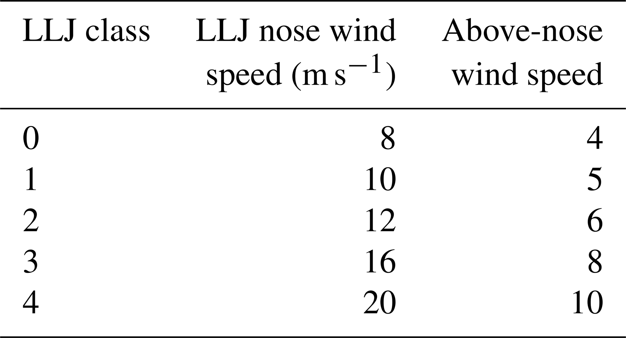
The observed and simulated temperature and wind profiles were linearly interpolated to an equidistant vertical grid with 10 m grid spacing. Profiles with less than 100 valid heights in the lowest 1500 m (corresponding to at least 1000 m in vertical coverage) were rejected. Then, the wind speed maximum in the lowest 1500 m was detected in each remaining hourly profile. This maximum had to occur in the lowest 700 m and exceed 8 m s⁻¹. This speed threshold was 2 m s⁻¹ lower than in Quint et al. (2025) and Bodini et al. (2026) because we found that many profiles that clearly showed an LLJ structure and were hence of interest for model development would have been missed otherwise. Above the nose, wind speed had to decrease by at least 4 m s⁻¹ to the next higher minimum or the 1500 m level, whatever is lower. We then classified the LLJ using five classes, based on the strength of the wind speed maximum at LLJ nose and above-nose wind speed decrease, following the pattern of Quint et al. (2025) and Bodini et al. (2026) but with an additional class to account for weaker LLJs (Table 1). Both thresholds need to be exceeded for an LLJ to fall into a certain class. For example, if LLJ nose wind speed is 17 m s⁻¹ and above-nose wind speed decrease is 5 m s⁻¹, the LLJ is classified as class 1, not class 3, because above-nose wind speed decrease does not exceed the threshold of 8 m s⁻¹ for class 3. We tested the sensitivity of our results to the nose wind speed threshold by performing the same analysis using a 10 m s⁻¹ threshold for nose wind speed, that is, only considering LLJs that fall into classes 1 through 4. While this reduced the number of LLJs in the data set, the model errors were largely the same when removing the weakest LLJ class.

Table 1 Criteria used for the classification of LLJs. Thresholds for wind speed at LLJ nose and above-nose wind speed decrease both need to be met.

To investigate the capability of the model to correctly predict LLJ we computed the critical success index:

$$\begin{array}{}\text{(2)}& \mathrm{CSI}={\displaystyle \frac{\mathrm{Hits}}{\mathrm{Hits}+\mathrm{False}\mathrm{positives}+\mathrm{Misses}}}.\end{array}$$

CSI of 1 indicates a perfect forecast. CSI can be high for very frequent events even without real skill or low for rare events despite model skill. We also computed the frequency bias:

$$\begin{array}{}\text{(3)}& \mathrm{FB}={\displaystyle \frac{\mathrm{Hits}+\mathrm{False}\mathrm{positives}}{\mathrm{Hits}+\mathrm{Misses}}}.\end{array}$$

FB of 1 indicates unbiased forecasts, values of less than 1 indicate an underestimation of frequency, and values larger than 1 indicate an overestimation.

We computed shear and static stability as the horizontal wind speed gradient and the virtual potential temperature gradient for the layer between 50 and 200 m. We chose 50 m as the lower boundary to at least partially mitigate the impact of the island and 200 m as the upper boundary because it was mostly below the LLJ nose. Virtual potential temperature θ_v profiles were computed using the dry-adiabatic lapse rate as

$$\begin{array}{}\text{(4)}& {\mathit{\theta }}_{\mathrm{v}}\left(z\right)=T_{\mathrm{v}}\left(z\right)+\mathrm{0.0098}\cdot z\end{array}$$

where T_v is the virtual temperature and z the height above ground.

As a measure of dynamic stability we computed the bulk Richardson number Ri (e.g., Stull, 1988):

$$\begin{array}{}\text{(5)}& \mathit{Ri}={\displaystyle \frac{g\mathrm{\Delta }{\mathit{\theta }}_{\mathrm{v}}/\mathrm{\Delta }z}{\stackrel{\mathrm{‾}}{{\mathit{\theta }}_{\mathrm{v}}}(\mathrm{\Delta }U/\mathrm{\Delta }z{)}^{\mathrm{2}}}},\end{array}$$

where g is gravitational acceleration, $\stackrel{\mathrm{‾}}{{\mathit{\theta }}_{\mathrm{v}}}$ is the layer-mean virtual potential temperature, $\mathrm{\Delta }{\mathit{\theta }}_{\mathrm{v}}/\mathrm{\Delta }z$ is the virtual potential temperature gradient, and $\mathrm{\Delta }U/\mathrm{\Delta }z$ is the wind speed shear. Shear, static stability, and Ri were computed for the layer below the LLJ nose as well as for constant layers using the boundaries detailed above. Negative Ri indicate a statically unstable environment. Small positive Ri indicate that the conditions are dynamically unstable, and large positive Ri indicate that the conditions are dynamically stable. The value to mark the transition between dynamically stable and unstable conditions depends on various factors, such as layer depth, growing or decaying turbulence, and near-surface vs. internal layers, and a transitional range spanning values from 0.25 to larger than 1 have been reported (e.g., Stull, 1988; Banta, 2008; Wittkamp et al., 2021).

3 Seasonal evolution of the marine boundary layer

3.1 Composites of temperature and wind profiles

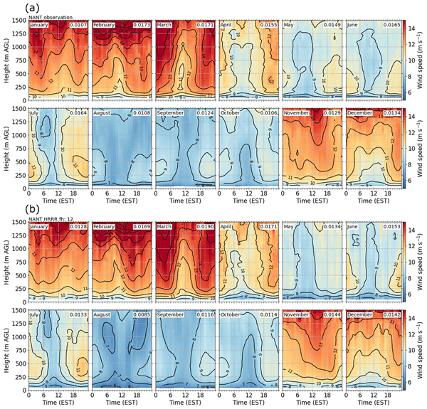
Monthly composites across the full diurnal range of observed horizontal wind speed (Fig. 4a) and potential temperature at NANT (Fig. 5a) show a strong seasonal cycle with generally higher wind speed during the colder months. A weak diurnal cycle in wind speed throughout the lowest 1.5 km was present on average with lower wind speeds during the day. Hardly any diurnal cycle in temperature was visible, except close to the surface, which likely represented the vertical extent of the internal boundary layer of the island at NANT. Above the internal island boundary layer, the marine boundary layer did not exhibit much of a diurnal cycle in temperature, which can likely be attributed to the damping impact of the water body on the marine boundary layer temporal evolution. Temperature stratification was statically stable on average with the strongest stability occurring in late spring and early summer (mean stability values are given in the upper right corner of each subplot in Fig. 5a). During these months, a low-level wind speed maximum in the lowest few hundred meters existed from late afternoon to early morning, indicating the occurrence of an LLJ (Fig. 4a). By visual comparison, the HRRR model did a very good job in capturing the seasonal and diurnal evolution of wind and temperature (Figs. 4b and 5b). Some differences are evident, especially during the warmer months, when low-level static stability and horizontal wind shear was too weak in the model on average, as indicated by numbers in the upper right corner of each subplot. For example, the observed average static stability in June was 0.0169 K m⁻¹, while it was only 0.0082 K m⁻¹ in the simulations, that is, it was underestimated by a factor of 2.

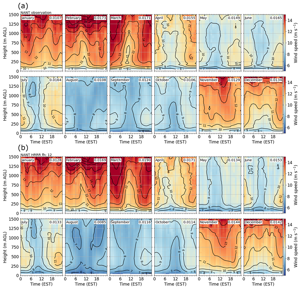
Figure 4 Monthly mean composites of (a) observed and (b) simulated horizontal wind speed (shading and contours) across the full diurnal range at NANT. In (b), forecast hour 12 of the HRRR model is shown. Only times and heights where both model data and observations were available were used for computing the composites, and availability had to be at least 25 % for a time/height pair to be plotted. The number in the upper right corner of each subplot indicates the monthly mean shear in s⁻¹ in the layer 50 to 200 m. Time is given in Eastern Standard Time (EST = UTC−5 h).

Figure 5 Monthly mean composites of (a) observed and (b) simulated potential temperature (shading and contours) across the full diurnal range at NANT. In (b), forecast hour 12 of the HRRR model is shown. Only times and heights where both model data and observations were available were used for computing the composites, and availability had to be at least 25 % for a time/height pair to be plotted. The number in the upper right corner of each subplot indicates the monthly mean static stability in K m⁻¹ in the layer 50 to 200 m. Time is given in Eastern Standard Time (EST = UTC−5 h).

Figure 6 Monthly mean composites of HRRR model errors (model minus observation) of (a) horizontal wind speed and (b) potential temperature across the full diurnal range at NANT. Forecast hour 12 of the HRRR model is shown. Availability had to be at least 25 % for a time/height pair to be plotted. Time is given in Eastern Standard Time (EST = UTC−5 h).

These errors in stability and shear were consistent with the composites of temperature and wind speed differences (Fig. 6). During the warmer months, the HRRR model underestimated wind speed by more than 1 m s⁻¹ on average in the lowest few hundred meters. During the colder months the underestimation of wind speed was less pronounced. The model overestimated temperature in roughly the lowest 200 m by up to a few degrees during the warmer months. This, in combination with an underestimation of temperature in the layers above, is consistent with the underestimation of low-level static stability (Fig. 5). The underestimation of low-level wind speed was similar to that observed far offshore on a barge that was deployed for WFIP3 during a few months in summer 2024 (Bodini et al., 2026). While wind speed errors at NANT did not show a distinct dependence on the time of the day, temperature overestimation below around 200 m was larger during the daytime hours during all months, especially during the summer. This diurnal variation in temperature difference indicates that there was an impact of the island topography at the site, with the HRRR model warming up too much during the midday hours over land in the lowest model layers. The general findings – a strong seasonal cycle and a weak diurnal cycle in observed horizontal wind speed and temperature and the frequent presence of an LLJ and statically stable stratification during the warmer months – also hold for the BLOC and RHOD sites (Sect. S4). The distinct low-level wind speed underestimation by the HRRR model was almost absent at RHOD (Fig. S8a) and weaker at BLOC where wind speed at the lowest height levels was even persistently overestimated (Fig. S5a). The overall overestimation of temperature close to the surface and an underestimation in the layers above by the HRRR model, especially during the warmer months, was also present at BLOC (Fig. S5b) and RHOD (Fig. S8b).

3.2 Dependence of model errors on forecast hour

In Sect. 3.1, only forecast hour 12 of the HRRR was investigated. In Figs. 7 and 8, bias and standard deviation of low-level wind speed and potential temperature dependence on forecast hour are shown per season. During the summer months (JJA), wind shear at NANT was too weak in all forecast hours (Fig. 7a), mostly caused by an underestimation of wind speed at 200 m by more than 0.5 m s⁻¹ (Fig. 7c). During the other seasons, no systematic biases in wind shear were found on average at NANT. At BLOC, wind shear was consistently too weak during all seasons for all forecast hours (Fig. 7a). This was largely caused by wind speed that was too strong at 50 m (Fig. 7b). This overestimation of 50 m wind speed could be related to the misrepresentation of the island topography in the HRRR model. At RHOD, average wind shear errors were small for all seasons and all forecast hours. Horizontal wind speed in the model was lowest at initialization time at individual height levels (50 and 200 m) and accelerated during the first few forecast hours, resulting in a decrease in bias (e.g., at 200 m at NANT and BLOC) or the evolution of a positive bias (e.g., 50 m at BLOC) (Fig. 7b, c). While the bias was relatively constant after the first few forecast hours, standard deviation of wind speed at 50 and 200 m increased with forecast hour for all seasons and all sites (Fig. 7b, c), indicating that forecast variability errors grew faster than systematic mean errors, likely linked to the general degradation of model skill with forecast hour.

Figure 7 Seasonal mean bias and standard deviation (STD) (HRRR model minus observation) of horizontal wind shear between 50 and 200 m and of horizontal wind speed at 50 and 200 m for forecast hours 0 to 18 at NANT and BLOC. Sample size is different for each site. DJF = December, January, February; MAM = March, April, May; JJA = June, July, August; SON = September, October, November.

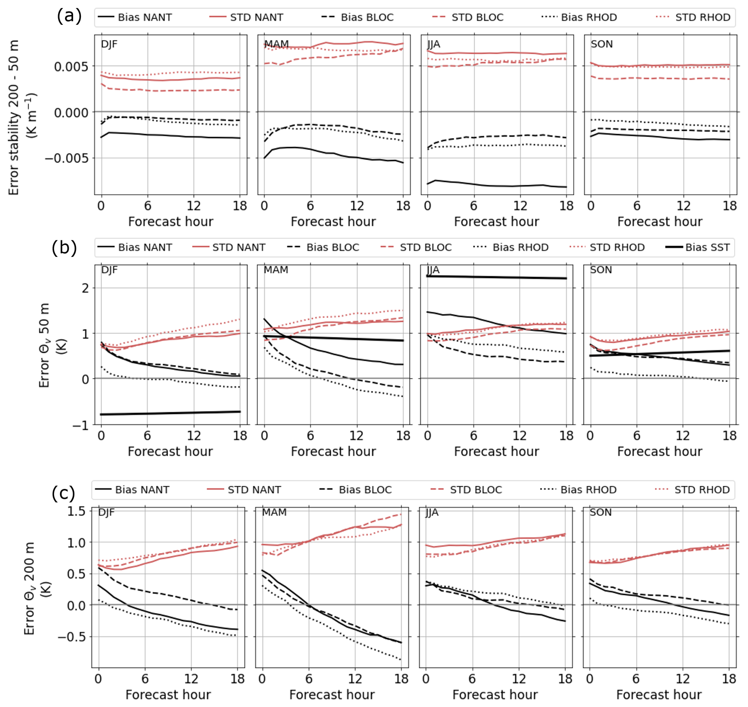
Figure 8 Seasonal mean bias and standard deviation (STD) (HRRR model minus observation) of static stability computed as the virtual potential temperature gradient between 50 and 200 m and of virtual potential temperature at 50 and 200 m for forecast hours 0 to 18. The thick black lines in (b) indicate the seasonal mean bias in SST at a grid point close to NANT. Sample size is different for each site due to different data availability. DJF = December, January, February; MAM = March, April, May; JJA = June, July, August; SON = September, October, November.

The bias in static stability, which was computed as the difference in simulated and observed virtual potential temperature gradient between 50 m and 200 m, showed that the model was not stable enough during all seasons and at all sites (Fig. 8a). Static stability was in particular too weak during spring (MAM) and summer (JJA). The errors in static stability can be linked to the errors at 50 and 200 m. At 50 m, temperature biases were mostly positive during all seasons. with the largest warm bias during MAM and JJA, and decreased in magnitude for longer forecast hours (Fig. 8b). At 200 m, the temperature bias was small and positive at initialization time and became negative for longer forecast hours (Fig. 8c). The combination of the sign of the errors at 50 and 200 m and their dependence on forecast hour, that is, the diminishing of a warm bias at 50 m and the growth of a cold bias at 200 m, resulted in stability errors that were nearly independent of forecast hour. The stability error was most pronounced at NANT, where SST was overestimated by more than 2 K on average during the summer months (JJA), which could contribute to the overestimation of 50 m temperature. This relationship will be investigated in more detail in Sect. 3.3. Similar to wind speed, the standard deviation at the two individual height levels (50 and 200 m) increased for longer forecast hours (Fig. 8b, c). In the following sections we will focus on forecast hour 12. Note that the general conclusions do not change for shorter or longer forecast hours, given the overall constant sign in errors for shear and stability.

3.3 Model errors in dependence of wind direction and SST errors

In this section, we investigate the relationship between HRRR model errors in wind speed shear and static stability and wind direction. Wind direction was generally well forecasted, with a mean absolute deviation of less than 15° at NANT and BLOC and approximately 20° at RHOD (not shown). The histograms of wind direction on the y-axis in Fig. 9a–c reveal that westerly flow was dominant and flow from the southeasterly quadrant was least frequent. This distribution agrees with results based on buoy-lidar data (Quint et al., 2025) or tower measurements (Kirincich et al., 2026).

Figure 9 Relationship between the error (HRRR model minus observation) in (a, d) horizontal wind speed shear between the 50 to 200 m layer and in (b, e) static stability computed as the virtual potential temperature gradient between 50 and 200 m layer and observed layer-averaged wind direction at NANT. (c, f) Relationship between the error in stability in the 50 to 200 m layer and the error in sea surface temperature (SST) (HRRR model minus OSTIA). The top row is for all available times, and the bottom row is when an LLJ is observed. Data at forecast hour 12 are shown for the HRRR model. Marginal axes show histograms.

Wind speed shear was both overestimated and underestimated at NANT depending on wind direction (Fig. 9a). The strongest underestimation occurred for southwesterly flow, mostly caused by an underestimation of 200 m wind speed (not shown). Other wind directions showed either a slight overestimation of shear (northwesterly flow) or no systematic errors (northeasterly flow). Static stability was predominantly too weak in the HRRR model. The largest stability error occurred for southwesterly flow (wind direction roughly between 180 and 260°). As shown in Sect. 3.2, the too-weak static stability was caused by a too-cold temperature at 200 m and a too-warm temperature at 50 m at this forecast hour.

To further understand the reason for the stability error, we more closely investigated the relationship between the errors in static stability and SST (Fig. 9c). These errors were weakly negatively correlated ($R=-\mathrm{0.3}$), meaning that static stability in the HRRR model was getting increasingly too weak with growing SST error. This was mostly linked to an overestimation of temperature at the bottom of the layer used for the static stability computation, that is at 50 m, where the SST and temperature errors were weakly correlated (R=0.3). This indicates that many of the cases with too-weak static stability in the model were linked to an overestimation of SST and consequently warm biased low-level temperature, suggesting that the specification of the lower boundary conditions are likely a contributing factor to the near-surface model errors. The relationship between stability errors, SST errors, and southwesterly flow indicates that those could be linked to coastal cold water upwelling that may occur under persistent southwesterly flow as shown by e.g. McCabe and Freedman (2026) for the New York Bight.

The largest errors in low-level wind speed and static stability occurred for southwesterly flow (Fig. 9a, b). These errors became even more visible when selecting only the samples when an LLJ was observed (Fig. 9d, e). The histogram of wind direction on the y-axis shows that southwesterly LLJs were most common, followed by northeasterly LLJs. This is in agreement with previous studies on LLJs in the area (e.g., Colle and Novak, 2010; Bodini et al., 2026). Most of the southwesterly LLJs were associated with an underestimation of wind speed shear (Fig. 9d) and static stability that was too weak (Fig. 9e). Northeasterly LLJs showed similar but weaker error. Consistent with the findings for all times, static stability was particularly too weak when SST was overestimated (Fig. 9f). While wind shear errors at BLOC (Fig. S9a, d) were similar to those at NANT, that is, the largest underestimation occurred for southwesterly flow, they were mostly caused by an overestimation of 50 m wind speed and not by an underestimation of 200 m wind speed, which could be related to the misrepresentation of the island topography as discussed before. At RHOD no systematic large shear errors were visible (Fig. S10a, d). Static stability errors were similar at BLOC (Fig. S9b, d) and RHOD (Fig. S10b,d), with the static stability being mostly too weak in the HRRR. Like at NANT, the stability error at BLOC was weakly negatively correlated with the SST error ($R=-\mathrm{0.1}$) (Fig. S9c, f). The lack of any correlation at RHOD (R=0.0) (Fig. S10c, f) may indicate that conditions at this site are too strongly impacted by land to be ideally suited to evaluate errors in the lower part of the marine boundary layer in the HRRR model. SST errors in the HRRR varied spatially (Fig. 3). While the SST was much too warm during the warmer months near NANT it was very well captured at the buoy location further south. Since SST has an impact on low-level static stability, stability errors in the HRRR model may thus be different in other parts of the investigation area.

4 Low-level jet characteristics and model errors

4.1 Low-level jet characteristics

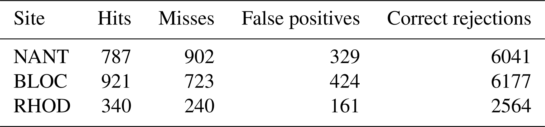
In the previous section, we showed that LLJs were often associated with relatively large systematic model errors (Fig. 9). This motivates a more detailed investigation of the observed LLJs and the ability of the model to predict them. The contingency table for observed and simulated LLJs is shown in Table 2, and statistics for LLJ characteristics are shown in Fig. 10.

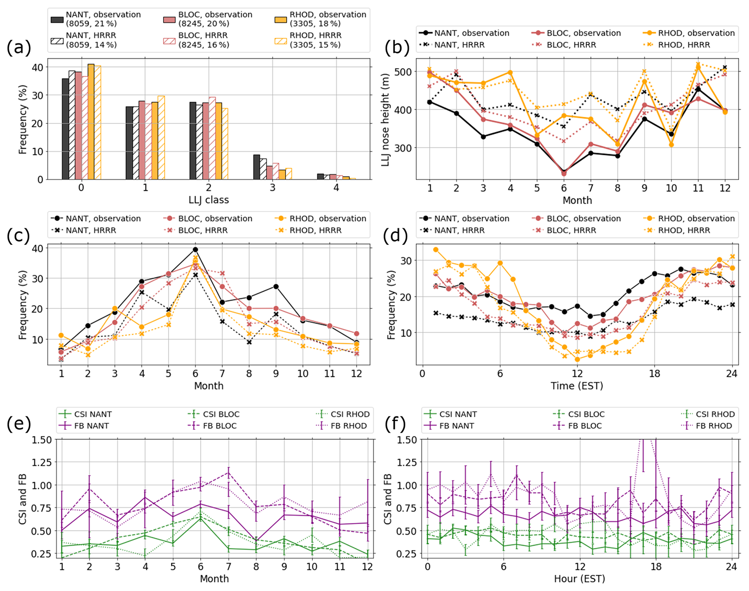
Figure 10 (a) Relative frequency of LLJ class, (b) mean LLJ nose height per month, (c) relative frequency of LLJ occurrence per month, (d) relative frequency of LLJ occurrence per hour of the day, and CSI (Eq. 2) and FB (Eq. 3) of the HRRR model per (e) month and (f) hour of the day at NANT, BLOC, and RHOD. The relative frequency of LLJ class in (a) is with respect to the times when a LLJ occurred and the relative frequency of LLJ occurrence in (c) and (d) is with respect to the number of valid profiles per month (c) and hour (d) that were available for LLJ detection. HRRR model data for forecast hour 12 are shown. Time is given in Eastern Standard Time (EST = UTC−5 h).

Table 2 Contingency table for observed and simulated (forecast hour 12) LLJs at NANT, BLOC, and RHOD. All LLJ classes are included.

LLJs were detected in 18 %–21 % of the observed profiles and in 14 %–16 % of the simulated profiles using only valid profiles with sufficient data availability (numbers in the legend of Fig. 10a). The percentage at RHOD was similar to NANT and BLOC despite the much lower number of valid profiles. About 35 %–40 % of all the observed LLJs in the area were classified as the weakest class 0, with a nose wind speed exceeding 8 m s⁻¹ and shear above nose exceeding 4 m s⁻¹. Class 1 and 2 LLJs occurred with similar frequency (each about 25 %–30 %). This distribution is fairly consistent at the three sites and captured well by the HRRR model. The monthly averaged LLJ nose height ranged between around 250 m in June to more than 400 m in the colder months, with the model overestimating LLJ nose height by 50 to 100 m on average (Fig. 10b). LLJ occurrence shows a clear seasonal cycle with more frequent occurrence during the warmer months from April to early summer (Fig. 10c), which was well captured by the HRRR model. In June, between 30 % and 40 % of all valid profiles had an LLJ shape independent of the site. LLJ frequency showed a secondary peak in September, especially at NANT, which was also present in the model, although underestimated. LLJs in September were predominantly associated with northeasterly flow (not shown) and likely linked to frontal passages. This distinguishes them from the LLJs that occur in late spring and early summer, which are predominantly from the southwest and likely driven by the land-sea temperature difference between the warm land and still cool ocean surface. Observed and simulated LLJ frequency ramped up in the afternoon and peaked during the first half of the night (Fig. 10d). The seasonal and diurnal cycle is in agreement with other studies on LLJs in this region (e.g., Aird et al., 2022; Quint et al., 2025) and can be explained by the diurnal heating and cooling of the land (Sect. 1). The diurnal cycle was most pronounced at RHOD at the coast with LLJs occurring less than 5 % of the time around midday. At NANT the diurnal cycle was weaker, with LLJ frequency not falling below 15 % in the observations. The HRRR model underestimated LLJ frequency at NANT pretty consistently by 5 %–10 % for all hours of the day.

The capability of the model to correctly detect LLJs is investigated by means of CSI and FB (Sect. 2.4). The HRRR model underestimated LLJ frequency, indicated by FB values less than 1 (Fig. 10e). The underestimation is larger at NANT than at BLOC and RHOD during the warmer months, with FB less than 0.75. This is consistent with the observed and simulated LLJ frequency in Fig. 10c. FB at NANT did not show a clear diurnal cycle (Fig. 10f), which means that the model did not systematically fail to predict LLJ profiles at a certain time of the day. At BLOC and RHOD, the model captured LLJ frequency best in the morning hours with FB values generally exceeding 0.80. CSI mostly ranged between 0.25 and 0.60, with the largest values in spring and early summer. In June, up to 60 % of the LLJ profiles were correctly predicted by the model at all sites.

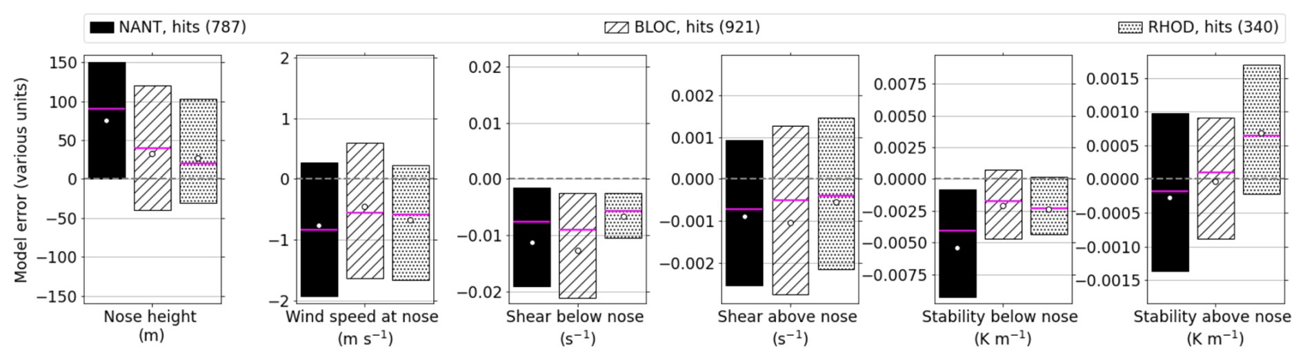
Figure 11 Box plot of HRRR model errors (model minus observation) at forecast hour 12 of LLJ nose height, wind speed at nose height, shear below nose height, shear above nose height, static stability below nose height, and static stability above nose height (from left to right) during LLJ hits at NANT, BLOC, and RHOD. The white circles indicate the mean biases, and boxes show the interquartile range with the median indicated by the horizontal pink line. Error units are given in brackets below each subplot.

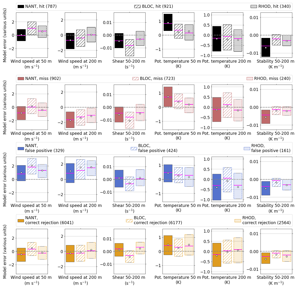
Figure 12 Box plot of HRRR model errors (model minus observation) at forecast hour 12 of wind speed at 50 and 200 m, wind shear between 50 and 200 m, potential temperature at 50 and 200 m, and virtual potential temperature difference (stability) between 5 and 200 m (from left to right) during LLJ (a) hits, (b) misses, (c) false positives, and (d) correct rejections. The white circles indicate the mean biases, boxes show the interquartile range with the median indicated by the horizontal pink line. Error units are given in brackets below each subplot.

4.2 Model errors during low-level jets

For a more detailed evaluation of HRRR model errors, we stratified the data for LLJ hits, misses, false positives, and correct rejections. Errors in LLJ nose height and shear and stability below and above the nose are shown for LLJ hits in Fig. 11. The model overestimates nose height by approximately 75 m at NANT, 40 m at BLOC, and 33 m at RHOD on mean average. Wind speed at nose height, wind shear below nose height, and wind shear above nose height are underestimated at all sites. The wind speed underestimation ranged between −0.5 m s⁻¹ at BLOC and −0.8 m s⁻¹ at NANT on average. The overestimation in nose height and underestimation of wind speed contribute to the underestimation in wind shear below nose height. The overestimation in nose height and underestimation in wind speed might be related to the relatively coarse vertical resolution with only 10 model levels below 1500 m. However, Li et al. (2021) found very little sensitivity of errors during LLJs to increasing the vertical or horizontal grid spacing. Below the nose, static stability is too weak at all sites on average, in particular at NANT. Above-nose static stability is also too weak at NANT on average, while it is too stable at RHOD.

The analysis of shear and stability errors is extended to LLJ misses, false positives, and correct rejections by looking at fixed heights (Fig. 12). Shear in the 50–200 m layer, which is usually below the observed and simulated LLJ nose height, was underestimated at all three sites for LLJ hits (Fig. 12a). The too-weak shear at NANT was caused by too-weak wind speed at 200 m, while at BLOC and RHOD an overestimation of the 50 m wind was mainly responsible. Static stability below 200 m was too weak, especially at NANT, which can be largely attributed to a warm bias at 50 m and a slightly cold bias at 200 m on average. Although wind speed was too weak during LLJ misses, the underestimation of shear was similar in magnitude to the LLJ hits (Fig. 12b). Not surprisingly, wind speed was overestimated during LLJ false positives, reducing the errors in shear (Fig. 12c). Static stability errors were negative at all sites for LLJ hits, misses, and false positives. This indicates that errors in the thermodynamic conditions were likely not the main reason for the HRRR to miss or falsely predict an LLJ. Many of the misses and false positives might be due to a misclassification when the minimum peak wind speed either in the model (misses) or in the observations (false positives) failed to meet the LLJ criteria. Wind speed and shear errors during correct rejections were smaller than during hits, which indicates the absence of large systematic wind speed errors outside of LLJ cases (Fig. 12d).

4.3 Bulk Richardson number regimes

To evaluate how well the HRRR model captures the dynamic stability during LLJ hits, we compute the relationship between horizontal wind speed shear and static stability below LLJ nose from the observations and simulations (Fig. 13a–c). Most of the observed and simulated LLJ profiles occurred under stably stratified conditions and were associated with positive low-level wind shear. In agreement with Fig. 11, the shear in the model during LLJ hits was too low. The model completely missed the high shear present in the observations. This resulted from the underestimation of wind speed at nose height, the overestimation of nose height (Fig. 11), and the overestimation of wind speed at 50 m (Fig. 12a). The frequency of profiles with weak static stability (<0.015 K m⁻¹) was overestimated, and the frequency of profiles with larger static stability (>0.015 K m⁻¹) was underestimated (Fig. 13a). Although the too weak shear partly compensated for the too weak static stability, the HRRR model still largely failed to produce low Ri (<0.5) conditions in the layer below the LLJ nose, especially at NANT and BLOC, which can be seen when comparing the frequency distributions of the observed and simulated Ri with the theoretical black lines in Fig. 13. This means that the model was too dynamically stable. In particular low Ri values that are associated with high shear values rarely occurred in the model. The observed Ri values at all sites are higher than what has been observed for continental LLJs, which is likely related to the weaker shear in the marine boundary layer. For example, Banta (2008) reported shear values below the jet nose of close to 0.1 s⁻¹ over the Southern Great Plains, resulting in Ri of around 0.1.

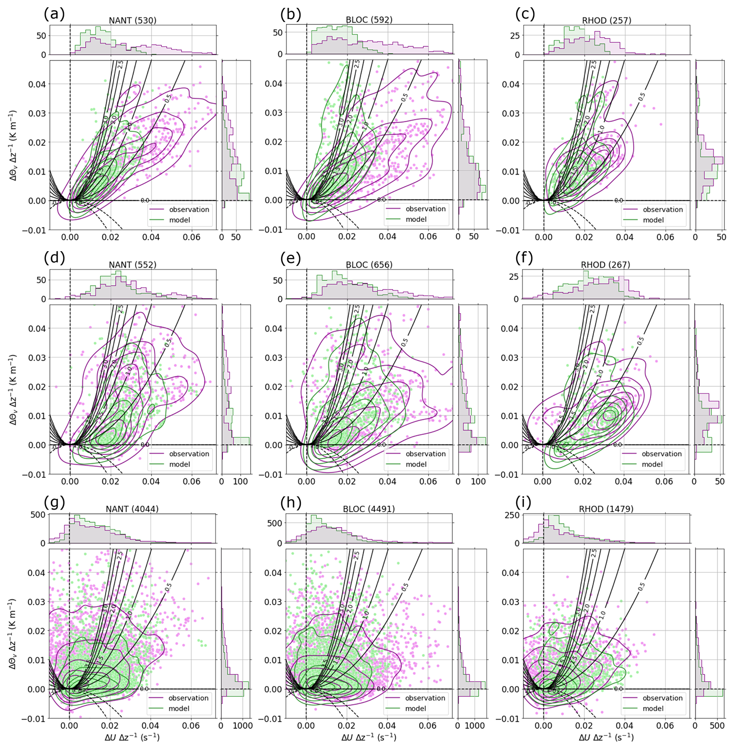
Figure 13 (a–c) Relationship between low-level static stability and horizontal wind shear for LLJ hits for gradients computed up to the LLJ nose height in the observations (purple) and HRRR model (green) at NANT, BLOC, and RHOD. Relationship between low-level static stability and horizontal wind shear in the layer between 50 and 200 m during (d–f) LLJ hits and (g–i) LLJ correct rejections. The number of samples is given in brackets above each subplot. Marginal axes show histograms. The black lines indicate theoretical Bulk Richardson numbers. HRRR data for forecast hour 12 are shown.

We also computed dynamic stability for fixed layers, which allowed us to compare the distributions of shear and stability during LLJ hits (Fig. 13d–f) and correct rejections (Fig. 13g–i). The distributions of shear and stability for fixed layers during LLJ hits (Fig. 13d–f) were similar to the ones computed for the layer below nose height (Fig. 13a–c) with the model missing profiles with strong shear at the three sites and underestimating the frequency of high static stability and overestimating lower static stability at NANT. During correct rejections, high shear (>0.03 m s⁻¹) and strong static stability (>0.015 K m⁻¹) were hardly observed and the HRRR model did well in capturing the distribution of shear and stability (Fig. 13g–i). In contrast to LLJ hits, when low Ri (<0.5) values occurred at moderate to large static stability and large shear values, low Ri values during correct rejections mostly occurred when static stability was weak.

The model discrepancies in representing correct Bulk Richardson number regimes likely originate from two primary factors: (1) suboptimal regulation of the Prandtl number, and (2) insufficient calibration of near-surface mixing intensity relative to surface stability. Regarding the former, the stability functions for momentum SM and heat SH within the MYNN-EDMF framework govern the proportional mixing of momentum and heat, as expressed by the Prandtl number $\mathit{Pr}=\mathrm{SM}/\mathrm{SH}$. When Ri>0.1, SM exceeds SH and can trend toward infinity as Ri surpasses 1. Refined management of momentum mixing in this regime is expected to mitigate the overestimation of weak shear and the simultaneous underestimation of strong shear. Concerning the latter factor, the magnitude of near-surface mixing in the MYNN-EDMF is chiefly governed by the surface layer length scale l_s, which is sensitive to the surface stability parameter $\mathit{\zeta }=z/L$. Here, L represents the Obukhov length (e.g. Stull, 1988) and z denotes the height above ground level. It is plausible that the regulation of l_s requires distinct treatment over marine versus terrestrial surfaces. Alternatively, the estimation of ζ could be re-evaluated using flux-profile relationships specifically developed for stable marine environments. Continued investigation into these mechanisms may address the systematic underestimation of shear and LLJ intensity, as well as the positive bias in LLJ nose heights. Other sources of errors could be associated with the bulk surface flux algorithm used over water (COARE3.0, Fairall et al., 2003), the detailed representation of the island soil temperature and moisture, and the representation of precipitation-induced surface sensible heat fluxes (Zhou et al., 2024a, b).

5 Summary and conclusions

This study evaluates the currently operational HRRR model (version 4) in the marine boundary layer along the northeast coast of the United States for a 1-year period from March 2024 through February 2025. The focus is on temperature and wind in the lower part of the boundary layer since an accurate forecast of this layer is most relevant for various applications such as marine transportation and fisheries, search and rescue, and energy production. We used unique continuous observations of temperature and wind profiles throughout the depth of the marine boundary layer at three sites, two of which were deployed on islands (NANT and BLOC) and one was deployed at the coast (RHOD) for the Third Wind Forecast Improvement Project. These data extended beyond the wind-only, buoy-based lidar measurements previously available in the region, which were limited to the lowest few hundred meters. The first part of the study focuses on the seasonal characteristics of the marine boundary layer and its representation in the HRRR model. The second part focuses on LLJs, since those were associated with large systematic model errors.

The main findings are:

• A strong seasonal cycle of wind and temperature was observed in the marine boundary layer, with strongest wind speeds occurring from November through March. The warmer months were characterized by the presence of a low-level inversion and an LLJ. The diurnal cycle was generally weak. While the HRRR model well captured the overall seasonal and diurnal evolution of temperature and wind in the marine boundary layer when computing monthly composites, some differences were evident, especially during the warmer months when the modeled low-level shear and static stability were too weak.

• Mean biases in low-level wind speed were generally less than 1 m s⁻¹ and did not grow much for longer forecast hours. They did, however, vary in sign by site with an underestimation at NANT, the site furthest away from the coast, and an overestimation at RHOD at the coast. Low-level shear errors were often small on the average at NANT and RHOD especialy during the colder seasons, but consistently underestimated at BLOC largely due to an overestimation of wind speed at 50 m, likely related to the erroneous representation of the island topography. Static stability was too weak in the HRRR model, with the largest errors during spring and summer. This resulted from a combination of too-warm temperatures at the bottom of the layer used for the stability computation and too-cold temperatures at the top. The too-warm temperatures at the bottom at the island sites were weakly linked to cases when the specified input SSTs were locally biased high. One possible reason for the too warm SSTs could be coastal cold water upwelling that was shown to impact sea breeze and associated LLJ structure in the New York Bight (McCabe and Freedman, 2026).

• The magnitude of wind speed and static stability errors revealed a strong dependency on the prevailing wind direction, especially at NANT and BLOC, with the largest underestimation of low-level shear and too-weak static stability occurring for southwesterly flow.

• LLJs were observed during around 20 % of all valid samples, with the highest frequency at NANT and the lowest at RHOD. Southwesterly LLJs dominated and were frequently associated with a large underestimation of low-level wind shear and too-weak low-level static stability. Although LLJs occurred throughout the year, they were most common during the warmer months from April to July when cooler SST allowed for the strong thermal land-sea contrast to develop that drives the LLJs in that area. Up to 60 % of the LLJs during peak season were correctly predicted by the HRRR model. The model skill decreased with distance from the coast and was lowest at the site furthest away from the mainland. About 40 % of all LLJs were classified as the weakest class 0. During LLJ hits, the nose height was overestimated and wind speed at nose height was underestimated on average, resulting in an overall underestimation of shear below nose height. HRRR model errors in low-level wind speed and shear were larger during LLJ hits than during LLJ correct rejections, indicating that systematic wind errors outside of LLJs were smaller. This is consistent with larger errors in dynamic stability during LLJ hits compared to correct rejections, with dynamic stability being too high during hits in the model.

We conclude that the HRRR's ability to forecast wind and temperature in the marine boundary layer is sufficient for most applications, but we identified LLJs as one atmospheric phenomenon with clear systematic errors. The too-weak static stability in the marine boundary layer during these events may allow too much vertical mixing, thereby reducing the horizontal wind shear. The stability error may be related to SST errors, and it is hypothesized that using an improved SST as input to the HRRR may lead to improved forecasts of wind and temperature, especially at the island sites. Other possible contributing factors could be the boundary-layer and surface-layer parameterization, land-sea mask representation, initial and boundary conditions, and errors in horizontal advection. As part of ongoing model physics development efforts at NOAA for the WFIP3 project, errors during LLJs have been alleviated, among others, in WRF-based model runs that use OSTIA as SST input and an experimental version of the MYNN-EDMF parameterization (Olson et al., 2026).