Km-scale regional coupled system in the Northwest European shelf for weather and climate applications: RCS-UKC4

Increasing the complexity of regional weather and climate models by developing coupled environmental prediction systems improves their performance, particularly in coastal areas where equilibrium assumptions between Earth system components break down. By allowing consistency between earth system components, they also unlock new insights on multi-hazard processes with benefits for enhanced forecasting. We present recent advances in the regional coupled environmental prediction system developed in the UK through the release of the Regional Coupled Suite – UK Coupled domain version 4 (RCS-UKC4) configuration. This includes implementation of the new Regional Atmosphere and Land configuration (RAL3.3) alongside updates to all model components relative to previous releases. RCS-UKC4 also supports enhanced online simulation of river flows and coupling to a biogeochemistry model. New functionality including running near-real-time ensemble forecasts and climate hindcasts is demonstrated. We first examine the effects of changing atmospheric and land configurations in both multi-annual simulations and short-term forecasts and assess the quality of river flows. RAL3.3 shows a beneficial increase in shortwave radiation reaching the ocean in summer months and a beneficial reduction in wind speed, which is slightly further reduced with wave coupling. Simulated river discharge has good skill in the northern and western regions of the UK, whilst there is too much variability for rivers in the southeast. Next, we introduce ensemble forecasts and show RCS-UKC4 has good wave forecast skill during storms compared to the current operational wave-only ensemble. This may partly reflect a good representation of tidal current/wave/wind interactions. Coupling can either increase or decrease the ensemble spread in screen temperature relative to atmosphere-only ensemble simulations, depending on whether latent heat flux or radiative heat flux dominates the spread in near-surface fluxes. Finally, we demonstrate that higher frequency (10 min coupling) enables new prediction capability with a good representation of high frequency sea surface height variability linked with weather disturbances.

1 Introduction

Coastal regions are complex environments and challenging for weather forecasting due to the strong influence of both land and sea (Cavaleri et al., 2018; Holt et al., 2017) with highly inhomogeneous land/sea geographical contrasts, strong tidal currents and areas of breaking, growing and reflecting ocean waves. On longer timescales, regional climate change is strongly modulated by a differential warming rate between land and sea (Kendon et al., 2010). Regional coupled systems are therefore increasingly being used for both weather forecasting (Durnford et al., 2018; Komaromi et al., 2021) and climate projections (Ruti et al., 2016; Somot et al., 2018), though their technical complexity and administrative separation of marine and land forecasts and projections restrict their widespread use (Berthou et al., 2025).

Berthou et al. (2025) highlight the many benefits of forecasts and projections enabled by consistent treatment of heat and momentum exchange in coupled systems. The United Kingdom is located on the Northwest European shelf (NWS), which is a shallow continental shelf sea region (< 250 m) where tidal energy is dissipated through strong tidal currents surrounding the British Isles. Deeper regions of the NWS become stratified in summer (e.g. North Sea), while shallower regions remain mixed throughout the column (e.g. Channel, Irish Sea). These strong tidal currents modulate wave height (Cavaleri et al., 2018) and even wind speed, which makes this region one of the few mid-latitude regions where the ocean dissipates tidal energy by modulating atmospheric wind (Renault and Marchesiello, 2022). In the mid-latitudes, the ocean feedback on the atmosphere remains weak, as pressure gradients are set by atmospheric baroclinicity, not by sea surface temperature (SST) gradients, and because deep convection is not a dominant driver of atmospheric variability. Nevertheless, it is now widely known that the ocean modulates the atmosphere at small time and space scales, such as over eddies, strong SST gradients and western boundary currents (Sheldon et al., 2017; Vannière et al., 2017). As high-resolution weather and marine forecasting have become more accurate, these interactions become non-negligible.

The Met Office currently operates a regional km-scale coupled wave/ocean deterministic forecast driven by its global coupled model (Guiavarc'h et al., 2019). This waves/ocean system shows benefits for predicting sea surface temperature (SST), surface currents during storms and extreme waves and surge (Bruciaferri et al., 2021; Lewis et al., 2019a). It's the forecast SST from this system now provide a time-evolving input to Met Office regional operational atmosphere forecasts. This change improved weather forecasts of air temperature during early summer and late autumn, when 5 d SST evolution is non-negligible (Mahmood et al., 2021), and has been shown to have particular benefit during marine heatwaves (Berthou et al., 2024). Passing hourly SST to the atmosphere also provided improvements to coastal fog forecasting (Fallmann et al., 2019).

These improvements to the operational system were enabled by development of a flexible research framework for km-scale regional coupling (Lewis et al., 2018, 2019b). Based on this system, Gentile et al. (2021, 2022) and Valiente et al. (2021) explored the benefits of coupling a wave model with the atmosphere and highlighted that a consistent treatment of momentum transfer between the atmosphere and the ocean is crucial for wave and wind forecasting, in particular during storms.

In this paper, we present an updated version of the Regional Coupled Suite – UK Coupled domain version four (RCS-UKC4), which brings corrections and enhancements relative to the UKC3 system. We document:

• a.

  the impact of upgrading the atmosphere and land configuration on the coupled system, demonstrating in particular the impact on prediction of SST, winds and river discharge;

• b.

  the introduction of ensemble forecasting capability, to show a regional coupled system offers potential for improved ensemble wave and wind forecasting, including discussion of options for further wind/wave improvements and how coupling modulates the ensemble spread of air temperature;

• c.

  sensitivity to increasing coupling frequency to 10 min and demonstrate this enables the ability to forecast meteotsunamis.

RCS-UKC4 also includes an option to couple a marine biogeochemistry model to represent the ocean colour, chemistry and lower trophic levels of biology (phyto- and zooplankton). The addition of a biogeochemistry system is further documented in a companion paper (Partridge et al., 2026).

2 Description of the coupled system

2.1 Updates in RCS-UKC4 from UKC3

Since UKC3 (Lewis et al., 2019b), the Regional Coupled Suite has been developed as a modular framework supporting fully or partially coupled simulations. It has primarily been applied over two model domains: one centred over India: RCS-IND1 (Castillo et al., 2022) and one over the United Kingdom: RCS-UKC4. Extending beyond deterministic case studies, the Regional Coupled Suite now supports running past or near-real-time ensemble forecasts (e.g. Gentile et al., 2022) as well as ability to run climate hindcasts.

RCS-UKC4 includes coupling the Unified Model (UM) atmosphere (Brown et al., 2012; Cullen, 1993), the Joint United Kingdom Land Environment Simulator (JULES) (Best et al., 2011), the Nucleus for European Modelling of the Ocean (NEMO) (Madec and the NEMO System Team, 2019), WAVEWATCH III (Tolman and the WWIII development group, 2014) and the European Regional Seas Ecosystem Model (ERSEM) (Butenschön et al., 2016) over a domain covering the Northwest European shelf (Fig. 1). The UM has a variable resolution from 4.4 km to either 1.5 km in deterministic forecasts (UKV) or 2.2 km in ensemble forecasts or climate runs (ENUK), on a rotated pole. NEMO and ERSEM share the same rotated pole domain as the atmosphere but using a regular ∼ 1.5 km fixed resolution grid (Graham et al., 2018). WAVEWATCH III uses a Spherical Multi-Cell grid for the same rotated pole domain, with 3 km spacing in the open ocean down to 1.5 km at the coast (Li, 2022). The UM and JULES are coupled at the timestep level as described by Best et al. (2004). The UM, NEMO and WAVEWATCHIII exchange fields through the Ocean Atmosphere Sea Ice Soil 3 – Model Coupling Toolkit (OASIS3-MCT) coupling library (Valcke, 2013), which handles the regridding and timing of field exchanges. NEMO and ERSEM are coupled with the Framework for Aquatic Biogeochemical Models (FABM) coupler (Bruggeman and Bolding, 2014), which handles 3D fields on the same grid. The additional biogeochemistry capability of the coupled system is documented in a companion paper (Partridge et al., 2026).

Figure 1 (a) UKC4 domain extent (same as UKC3), ocean bathymetry and orography. Orange dotted line shows the atmospheric inner domain with 2.2 km resolution, outside this domain, the atmosphere runs on a 4.4 km × 4.4 km grid in the corners, and mixed 4.4 km × 2.2 km in the outer middle sections. The ocean has a regular 1.5 km grid, the waves have variable 3–1.5 km resolution, 1.5 km close to the coast. (b) Hydrodynamic regions of the domain as defined by Wakelin et al. (2012), regions 1–11 delineate the Northwest European shelf.

Compared to UKC3, all component models have been upgraded to the state-of-the-art code versions:

• UM v13.5, with options of running three Regional Atmosphere and Land configurations: RAL1 (Bush et al., 2020), RAL2 (Bush et al., 2023) or the newest RAL3.3 (Bush et al., 2025), requiring additional branches in UM v13.5¹. Note that in this paper, RAL3.2 is also sometimes used, as the latest available version when some documented experiments were conducted. The main difference between RAL3.2 and RAL3.3 relevant to this paper is an increase in low-level cloud cover in anticyclonic conditions from changes in monotonicity scheme for moisture advection, and further changes to make the radiation scheme more consistent with the use of CASIM microphysics (Bush et al., 2025).

• JULES v7.5, with an additional JULES branch¹ to run online river routing with the River Flow Model (RFM). Online RFM was implemented and documented by (Lewis and Dadson, 2021).

• NEMO v4.0.4 for the Atlantic Margin Model 1.5 km (AMM15) domain (Patmore et al., 2023), with a change to the light penetration fraction to use same value as in Met Office operational wave/ocean coupled forecasts (Tonani et al., 2019, see also Sect. 3.1).

• WAVEWATCH III v7.12 (Tolman and the WWIII development group, 2014)

• ERSEM v15.06 (Butenschön et al., 2016)

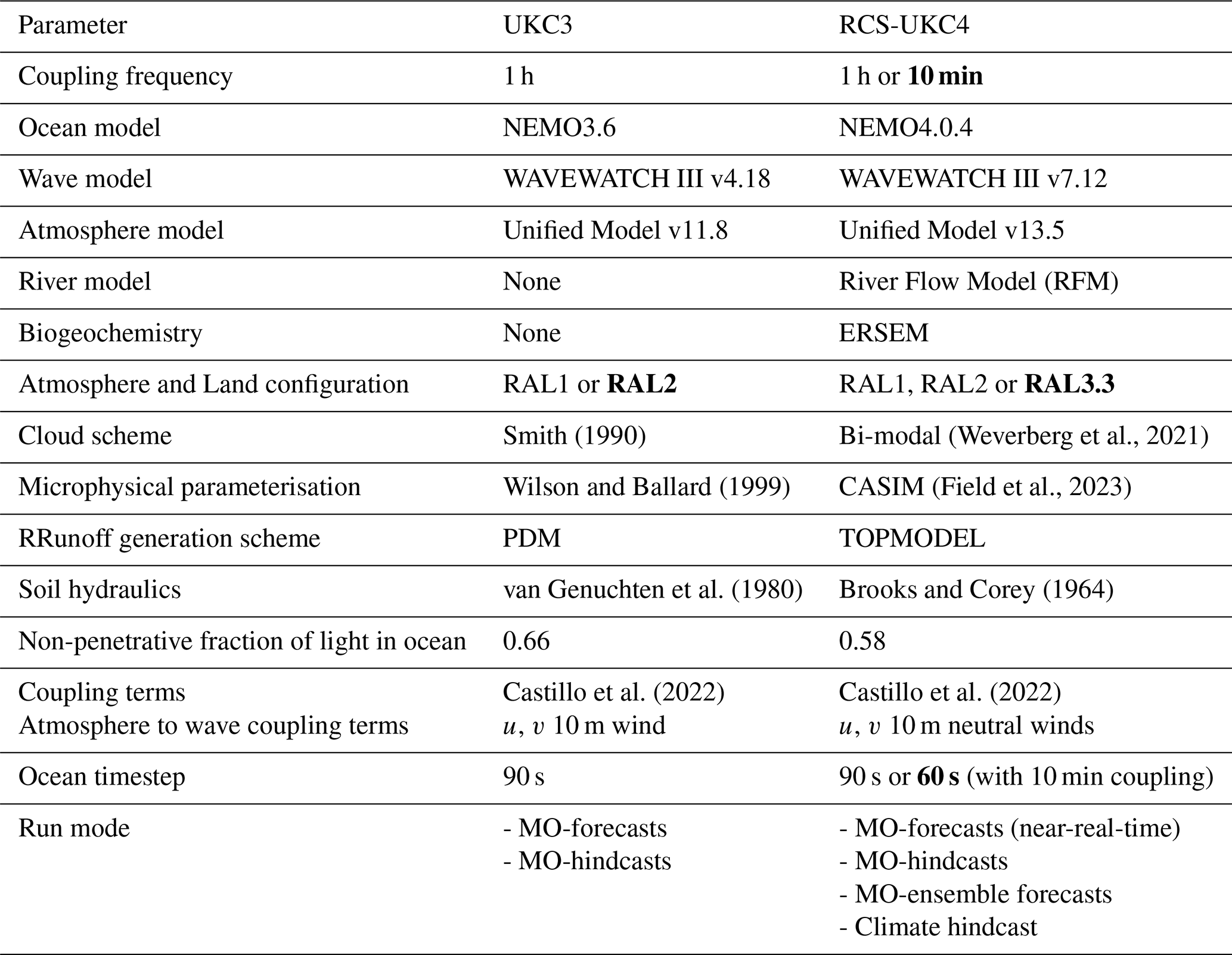
In a coupled system, changes in one component will inevitably affect the others: this article documents the journey undertaken from changing individual model versions and science configurations to having a final updated coupled system. Table 1 shows the main differences in UKC4 compared to UKC3, focusing on changes to the model science configuration most relevant to this work: the full set of changes is documented in Tables 1 and 2 of Bush et al. (2025). Details of the coupling terms are documented by Castillo et al. (2022), with the only subsequent update to exchange 10 m neutral winds instead of actual 10 m winds (see Sect. 3.2). The coupling frequency has also been increased from 1 h to 10 min (see Sect. 4).

Table 1 Summary of changes from UKC3 to RCS-UKC4. Where multiple options are supported, note the default set-up is indicated in bold.

2.2 Run modes: deterministic, ensemble forecasts and climate runs

UKC3 could be forced by operational forecast lateral boundary conditions (LBCs) and initial conditions (ICs), with options to either generate past forecasts (MO-forecasts) or to run using LBCs from the latest available valid global forecast each day (MO-hindcast). This was limited to the period from 2018 onwards, when individual components of the coupled system first became operational (AMM15 ocean and waves).

The RCS was developed to accommodate more ways to running the system:

• MO-forecasts (as in UKC3), including the new option to run near-real-time forecasts using operational LBCs directly from disk, rather than retrieving post-event from the archiving system.

• MO-hindcast (as in UKC3), with updated LBCs every day taken from the latest available global forecast initialised at 00:00 UTC (all times in UTC), supporting longer runs beyond typical operational forecast length (e.g. Berthou et al., 2024; Partridge et al., 2026).

• MO-ensemble forecasts, based on the work from Gentile et al. (2022): 18-member ensemble integrating the Met Office Global and Regional Ensemble Prediction System over the United Kingdom (MOGREPS-UK; Porson et al., 2020) atmosphere-land ensemble forecast with the regional ocean-wave system. The ensemble includes one unperturbed reference simulation and 17 perturbed members, where atmospheric initial and lateral boundary conditions are generated by downscaling perturbations from the global MOGREPS-G system. Each regional atmosphere member also includes stochastic physics perturbations. While atmosphere members are initialised from different global ensemble members, the ocean and wave components start from the same deterministic operational ICs. While the ocean/wave components generate some perturbations in the coupled system, additional SST and land temperature perturbations are applied to the atmosphere component following Tennant and Beare (2014). These MOGREPS-G SST perturbations are applied through the OASIS coupler only and implemented such that they are fixed for the forecast duration with an average of 0 °C across all ensemble members and maximum local amplitude of 2 °C.

• Climate hindcast (driven by LBCs from ERA-5 for the atmosphere (Hersbach et al., 2020), GloSea5 for the ocean (MacLachlan et al., 2015) and an ERA-5 driven global Met Office wave standalone hindcast for the wave, similar to the EU Copernicus Marine Service Information (CMEMS) Wave physics reanalysis (2025)).

• Climate projections (driven by a global climate model, but not documented further in this paper)

Known Good Outputs (KGO) have been added as benchmarking cases to ensure new changes in the Regional Coupled Suite do not break capability. Optimisation tests have been run to reach a balanced system with individual components running at the same speed.

2.3 Evaluation strategy

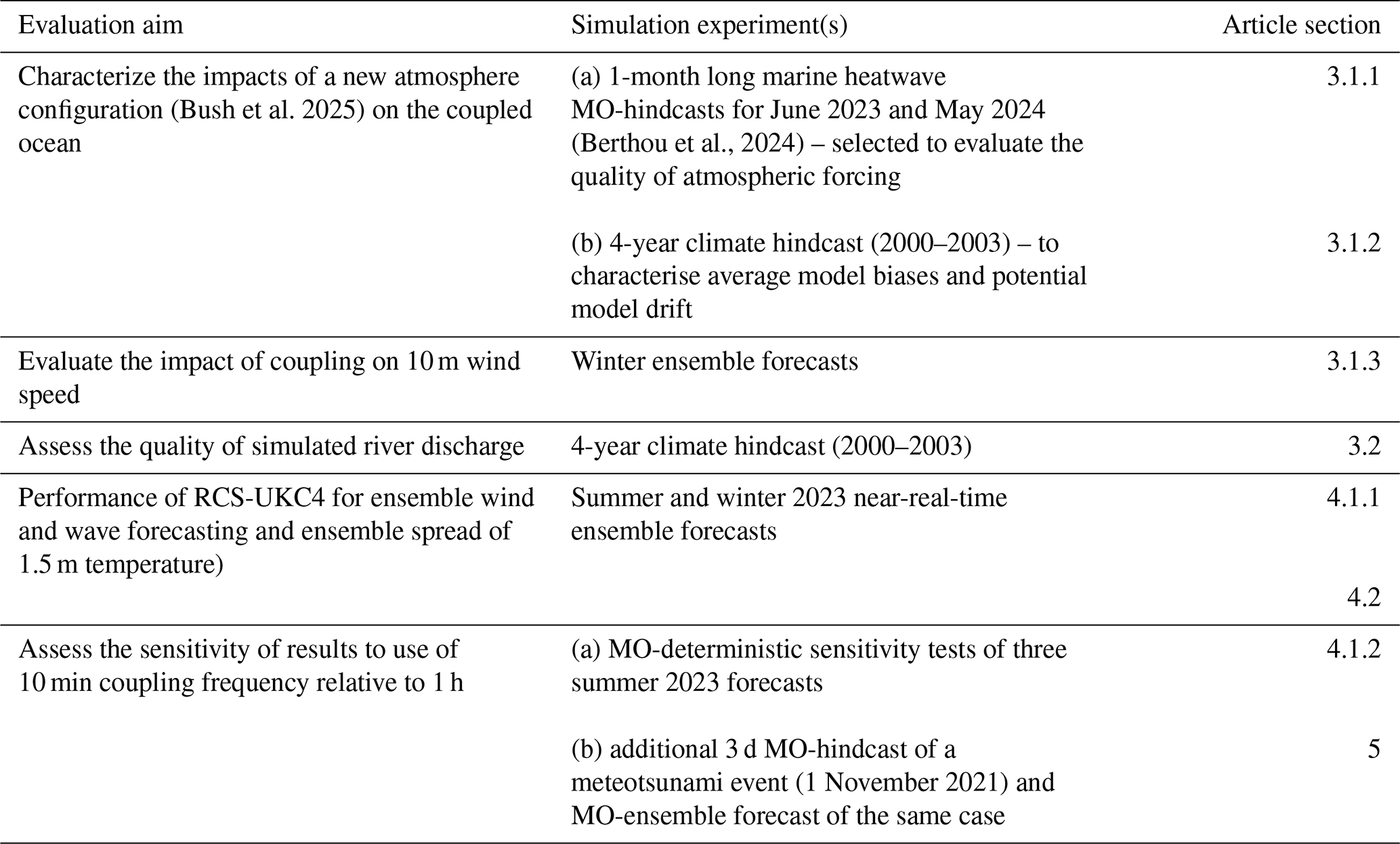
Evaluation of the coupled system has exploited the variety of run modes across, weather and climate timescales and atmosphere, river, ocean and wave components (Table 2).

Table 2 Summary of RCS-UKC4 evaluation and supporting simulation experiments, details of each set of experiments is given in Table 3.

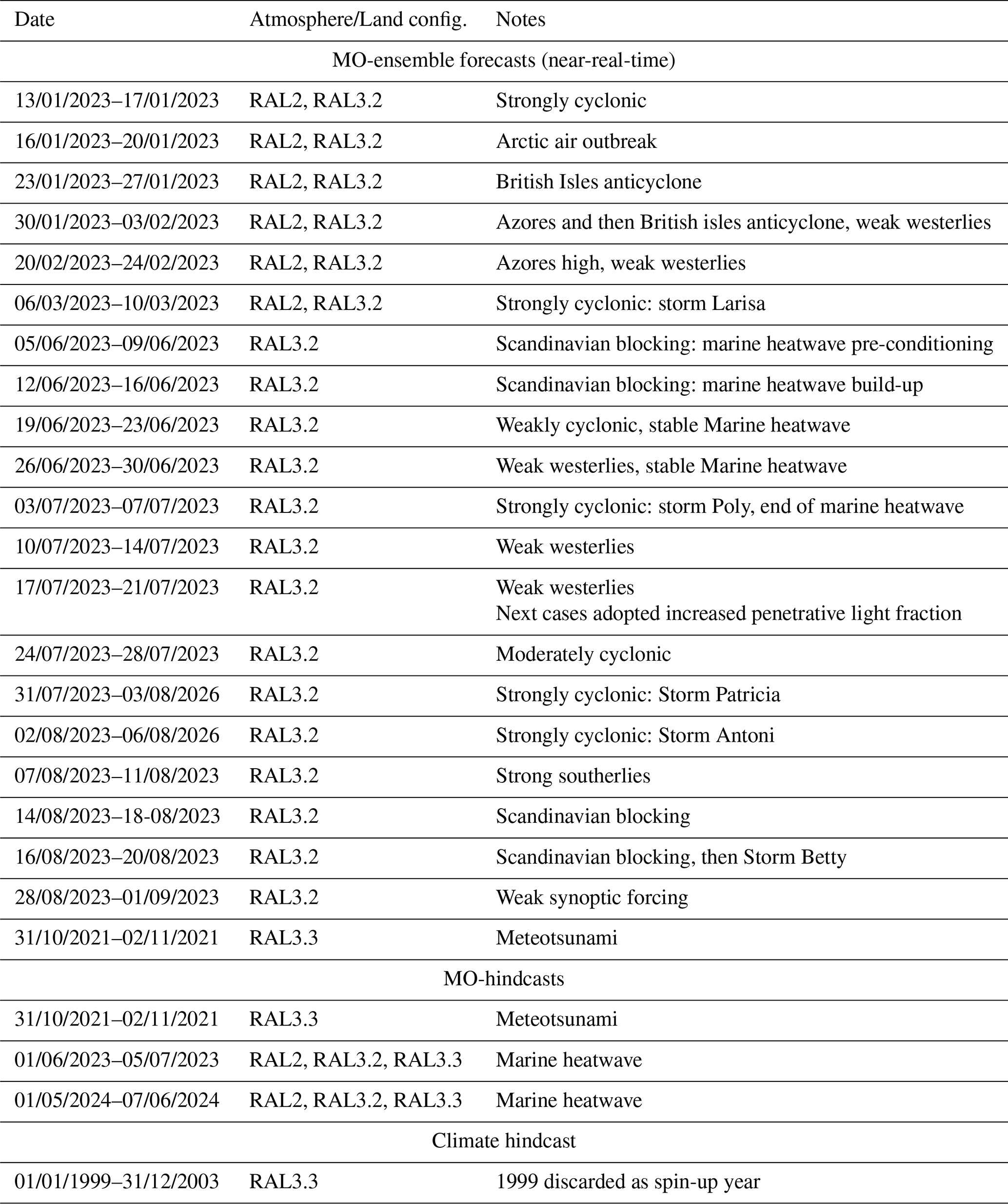
We performed two near-real-time ensemble trials to support RCS-UKC4 evaluation: one in winter 2023 and one in summer 2023 (Table 3). Winter 2023 was characterized by cold and anticyclonic weather regimes in January cases and one named storm (Larisa) in March in the English Channel. The summer ensemble was run weekly every Monday during the WesCon field campaign in the UK (Barrett et al., 2021), from 5 June to 21 August. The month of June was characterized by weak synoptic forcing: anticyclonic regimes for the first two weeks and weakly cyclonic regimes in the last two weeks. Exceptionally strong sunshine and weak waves generated an intense and long (1 month) marine heatwave over the Northwest European shelf (Berthou et al., 2024). The month of July and first two weeks of August were dominated by strong cyclonic circulation, with three named storms: Patricia, Antoni and Betty. The last two weeks of August had weaker circulation and a few sea breeze days.

Table 3 Details of RCS-UKC4 experiments run for model evaluation

3 Improving model components

3.1 Impacts of changing the atmosphere and land configurations on the coupled system

3.1.1 Performance in marine heatwave conditions

We tested the impact of an updated atmosphere configuration in RCS-UKC4 for two recent marine heatwaves (June 2023 and May 2024). Marine heatwaves provide an effective test case for coupled systems. as they often show an extreme stratification at the ocean surface. The ocean mixed layer can be very shallow (Berthou et al., 2024) and any errors in the heat flux budget in a coupled system will translate into large SST errors. The new atmospheric configuration (RAL3.3) leads to warmer SSTs than RAL2, with clear improvements for May 2024, and a shift from a cold (as much as −0.5 °C) night-time SST bias in June 2023 to a warm (up to 0.3 °C) bias averaged over the northwest European shelf (Fig. 2). Note that the Operational Sea Surface Temperature and Ice Analysis (OSTIA) is a foundation SST product (Good et al., 2020), so in our interpretation of this figure, we compare it to the model's minimum diurnal temperature. The additional cloud/microphysics tuning between RAL3.2 and RAL3.3 is beneficial in June 2023 but has little impact in May 2024. The main difference in SST in June between atmosphere configurations comes from a difference in shortwave radiation, as further changes were implemented to increase stratocumulus cloud cover in anticyclonic conditions, judged too low in RAL3.2 by forecasters (Bush et al., 2025). The RAL3.3 cloud/microphysics tuning showed little impact on shortwave radiation for the May 2024 simulations, potentially because conditions were not as favourable for stratocumulus formation.

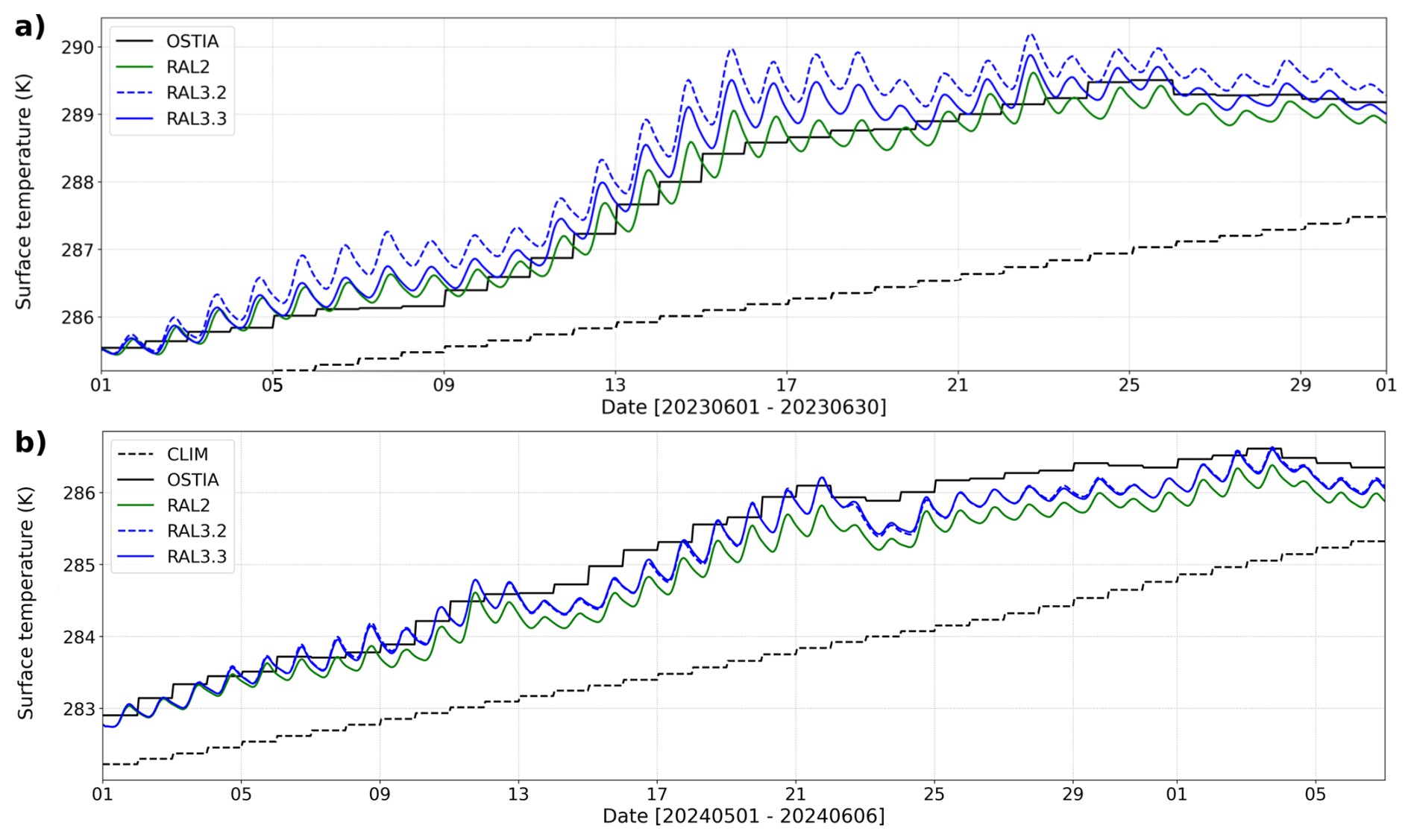
Figure 2 Sea surface temperature averaged over the Northwest European shelf (delineated in Fig. 1b) for (a) June 2023, (b) May 2024 (1 May 2024 to 6 June 2024) in OSTIA (black line), its 1982–2012 climatology (black dotted line), and the coupled system with RAL2 (green line), RAL3.2 (blue dotted line) and RAL3.3 (blue line) atmospheric configurations.

Because of the limitations of satellite SST products (limited by cloud cover, and night-time surface temperatures), we complement this analysis with a comparison of RAL2 and RAL3.3 against in-situ ocean temperature observations, usually taken at 0.5 m depth. This is consistent with the first model level of AMM15. Figure 3 shows the average bias against in-situ SST observations available in the Met Office observation archive (including ships, buoys and sea platforms) for May 2024 and June 2023. Results confirm the tendency of RAL2 to have a cold bias, and for RAL3.3 to reduce this bias: it is clear in May 2024 (Fig. 3b, d) and in the Channel and Southern North Sea in June 2023, though RAL3.3 shows a warm bias in the Northeast Atlantic, the Celtic Sea and the North Sea in June 2023 (Fig. 3a, c). Nevertheless, even in places where RAL3.3 degrades from RAL2, the warm bias in June 2023 rarely exceeds 1.5 °C. Figure 4 shows the impact on 1.5 m air temperature: RAL3.3 is mostly an improvement over RAL2, except for the Celtic Sea and west of Scotland in June 2023. Notably, despite the warm sea surface bias in part of the domain in June, the air temperature still has a cold bias, in the North Sea, the Irish Sea and the Channel. In this particular marine heatwave, the atmospheric boundary layer was very shallow. This cold air bias suggests sensible heat fluxes may be too weak in RAL3.3 in low wind conditions. This will need assessing in future model development.

Figure 3 Mean sea surface temperature bias against in-situ ships and buoys averaged over the month of June 2023 (a) and May 2024 (b). Bias improvements from RAL2 to RAL3.3 (%) (c, d). Observation only used if recording more than 10 values over the simulation time.

Figure 4 Same as Fig. 3 for 1.5 m air temperature.

Because of these results, the light penetration (66 % of radiation applied to the first model level, and 33 % penetrating deeper in UKC3) was tuned back to 58 % applied to first model level, 42 % penetrating (RCS-UKC4). This cooled the SST by ∼ 0.2 °C in the June 2023 marine heatwave (not shown). This light penetration value is now the same as the operational AMM15 model (Tonani et al., 2019). Note that this value is spatially and temporally homogeneous, which is unrealistic, given the difference in ocean colour between turbid river plumes and tidal regions, “greener” phytoplankton bloom season and “bluer” winter/summer season. Using a time and space varying light treatment is planned in a future release (e.g. feedback from ERSEM to NEMO, as in Skákala et al., 2022).

Overall, the evaluation of RCS-UKC4 in marine heatwave conditions is consistent with an improved surface fluxe budget in RAL3.3. This is inferred from the evaluation of the SST when the ocean surface mixed layer is shallow: although no direct measurement of the heat budget was made over the sea, the SST is highly dependent on the quality of surface fluxes in these conditions (Berthou et al., 2024). These results contributed insights from the RCS, for the first time, in decision-making in the development cycle of the Regional Atmosphere and Land configuration (Bush et al., 2025).

3.1.2 Evaluation of SST in RCS-UKC4 climate simulations

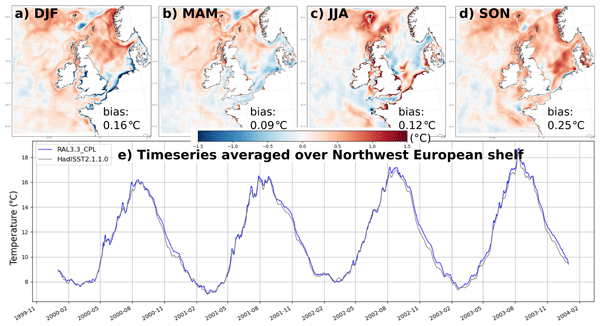
Evaluating multi-year simulations is essential for a coupled system, as any seasonal cycle imbalance in surface fluxes can bring large model biases or induce year-to-year drift in SST. Here, we evaluate the quality of the sea surface temperature in 4-year long simulations, for which the SST quality will both depend on the atmospheric fluxes and the ocean dynamics. Figure 5 shows that the 4-year mean bias in all seasons is always smaller than 1.5 °C (away from the coastline, where HadISST is not reliable). Spring and summer show smaller biases (0.09–012 °C averaged across the whole domain), while autumn and winter have a warm bias of around 0.16–0.25 °C. This warm bias persists throughout the seasons in the deeper northwest part of the domain. The coupled system evidently generates abundant fine-scale detail near coastal regions, but their evaluation is challenged with low-resolution satellite-based SST products. In the autumn, ocean cooling is dominated by entrainment and latent heat cooling, both related to wind speed: this autumn bias may be linked to an underestimation of the strongest wind speeds in RCS-UKC4 (see Sect. 4): the cooling episodes of October-December are not strong enough, though the warm bias eventually disappears at the coolest stage (February–April). Nevertheless, the results indicate acceptable biases for the SST in a free-running coupled system. The biases do not grow over time, which is also a sign of good quality. Further evaluation of this climate run will be discussed in a future paper, but this preliminary evaluation shows the RCS-UKC4 configuration is acceptable for both forecasting and climate modelling of the SST.

Figure 5 Sea surface temperature of the hindcast run (2000–2003) for HadISST2.1.1.0 and coupled model, (a) SST bias averaged over December-January-February (DJF) 2000–2003, (b) SST bias averaged over March–April–May (MAM), (c) SST bias averaged over June–July–August (JJA), (d) SST bias averaged over September, October, November (SON) and (e) SST averaged over the Northwest European shelf for (blue) UKC4 and grey HadISST2.1.1.0.

3.1.3 Changes in wind speed

A series of ensemble forecasts in winter 2023 using RAL2 (uncoupled) and RAL3.2 (uncoupled and coupled) atmosphere configurations to evaluate the impact of coupling on wind speed over the sea in different weather conditions. Note results are expected to still be valid with RAL3.3 given the microphysics/cloud tuning from RAL3.2 to RAL3.3 is not likely to impact wind speed, the rest of the section will refer to RAL3.

Gentile et al. (2021) documented a 10 %–20 % wind decrease when coupling to waves in stormy conditions compared to uncoupled RAL2 experiments. This was partly due to different drag parameterisations between RAL2 and WAVEWATCH III source-term 4 (WWIII-ST4). The relationship between the drag coefficient and wind speed depends on the Charnock coefficient and atmospheric stability functions. The drag increases with wind speed faster in WWIII-ST4 than in RAL2, which uses a constant Charnock value (0.011). This difference resulted in a tendency of a wind decrease in coupled simulations, in particular in cases with strong winds (Gentile et al., 2022). Gentile et al. (2021) recommended to upgrade the atmosphere-only drag scheme to COARE4.0 with (Donelan, 2018) cap, which was adopted in RAL3, and is closer to the WWIII-ST4 parameterisation: in RAL3, Charnock shows a linear growth with wind speeds, capped at 22 m s⁻¹, which effectively models an empirical weak dependence of the parameter on the wave age. These differences in drag/wind relationship and the change in spread due to coupling is also evident in the ensemble probability of wind speed (Fig. 6). At moderate wind speeds (illustrated in Fig. 6b, c), results are consistent with Gentile et al. (2022): young, growing waves extract momentum from the atmosphere and coupling reduces the wind speed, in particular in the sheltered North Sea. This is well illustrated in Fig. 6a, where the spread in the drag is increased towards higher values compared to atmosphere-only for 10 m s⁻¹ values. For storm-force wind speeds (20 m s⁻¹), the probability of reaching such wind speeds is slightly higher in coupled mode (Fig. 6d, e), as the drag coefficient is reduced in some regions by wave coupling for these wind speeds (Fig. 6a).

Figure 6 Panel (a) shows the 10 m neutral drag coefficient as a function of 10 m wind speed for RAL3.2 (grey), UKC4 (yellow), and RAL2 (blue) on 10 March 2023. Probability of wind speed > 10 m s⁻¹ on 10 March 2023 at 01:00 UTC during storm Larisa (b, c), > 20 m s⁻¹ (d, e) for atmosphere only with RAL3.2 configuration (a, c), UKC4 (c, e). The black oval indicates the region with the largest differences.

Comparing wind biases against observations for atmosphere-only simulations using RAL2 and RAL3 to coupled RCS-UKC4 output (Fig. 7) highlights that RCS-UKC4 is indeed more similar to RAL3 than RAL2. There is little difference between experiments for the 23 January 2023 case, as it is dominated by weak wind conditions for which there are smaller sensitivity of the drag coefficient (Fig. 6a). In all the other cases, characterised by stronger wind speeds, the biases are better centred around 0 for atmosphere-only RAL3 and coupled RCS-UKC4 compared to atmosphere-only RAL2, with reduced positive biases but sometimes enhanced negative biases. This illustrates that results are more sensitive to changing the slope of the drag/wind relationship than coupling. The main effect of coupling is to enhance the spread around the drag/wind speed relationship, by introducing a wave-state dependency (Fig. 6a). This is particularly important in the vicinity of complex coastlines where reflection and sheltering effects mean waves are not always in equilibrium with the wind state. The reduction of moderate wind speeds with wave coupling over the sea has an impact on coastal winds, with a ∼ 0.1 to 0.2 m s⁻¹ reduction in ensemble mean wind speed in all four cases (not shown).

Figure 7 Histogram of wind biases against all buoys for four different winter 2023 cases, an indication of duration of strong wind speeds averaged over the sea part of the domain is given on each figure (length of time when at least a few members reach a domain-average mean wind speed of 10 m s⁻¹).

3.2 Quality of the river flows

Following Lewis and Dadson (2021), river routing has been implemented in RCS-UKC4 using the River Flow Model in JULES (see Appendix B of Lewis et al. (2018). The RAL3 configuration in RCS-UKC4 uses a 1D groundwater model (TOPMODEL; Gedney and Cox, 2003) to represent the generation of runoff in the soil column, in contrast to the Probability Distributed Model (PDM, Moore, 1985) used in RAL2 (and used in Lewis and Dadson, 2021). In both configurations, a saturation excess runoff is calculated by JULES, increasing with rainfall intensity (Best et al., 2011). With PDM, the additional surface runoff depends on the saturation of the first two layers of soil while in TOPMODEL, surface runoff is a function of whole soil column saturation and local topographic variability. Subsurface runoff is calculated by PDM as water drainage at the bottom of all soil layers, while in TOPMODEL this depends on water content below the calculated water table depth, and a topographic index, which relates to the upstream area draining into a locality and the local slope. In general, PDM tends to generate more surface runoff, while TOPMODEL generates more subsurface runoff. The River Flow Model then routes surface and subsurface runoff with different wave speeds: 0.5 m s⁻¹ for surface runoff and 0.05 m s⁻¹ for subsurface runoff. These are currently set as constants across the whole domain.

Figure 8 shows evaluation metrics of the daily model flow against the National River Flow Archive (NRFA) gauges. For each gauge location, the model grid point with the catchment area closest to that of the gauge was identified from among the nearest grid cell and its surrounding 24 grid points. Nash-Sutcliffe efficiency (NSE; Fig. 8b) is defined as one minus the ratio of the error variance of the modelled time-series divided by the variance of the observed time-series. Negative values mean model has worse skill than prediction based on average observed flow, values above 0 show model has skill in both mean and variability, and values close to 1 show perfect model. RCS-UKC4 results show negative NSE across most of the south-east England, whereas it ranges from 0.2 to 0.8 in the southwest and north of the UK. To understand the model performance, we further show the three components of the Kling-Gupta efficiency: normalised bias, ratio of model and observation variances, and Pearson correlation coefficient (Fig. 8a, c, d). The bias is mostly negative, ranging from 10 % to 60 % underestimation. It is strongest in the west and decreases east, closest to 0 in the southeast. The ratio of variance clearly shows an overestimation of flow variability in south-east England and an underestimation in the southwest, west and north of the UK. Similarly to NSE, the correlation between observed and modelled flows is close to 0 in the southeast and ranges between 0.4–0.8 in other parts of the UK. Southeast catchments are usually connected to groundwater aquifers and have long time-responses: they are dominated by baseflow.

In other regions, catchments are flashier, with faster response rivers. This is illustrated in timeseries of the largest UK catchments (Fig. 9). Catchments in the west and north show too much baseflow, and underestimated extreme values (Fig. 9a, b, c, e). The amplitude of the annual cycle is too small, with underestimated winter peaks, and overestimated summer peaks. In contrast the two southeast catchments (Fig. 9d, f) show too much variability and not enough baseflow. This illustrates that TOPMODEL tends to keep too much water locked in the soil in winter, slowly released as baseflow in spring and summer in the west and north of the country. In these regions, soil is not always as deep as 3 m, as assumed by JULES: Weedon et al. (2023) recommended reducing saturated conductivity to very low values in deeper parts of the soil in these areas, which would reduce soil capacity to store water. Weedon et al. (2023) also showed that JULES with TOPMODEL had too much surface runoff in the southeast UK, and recommends using large values of saturated conductivity, based on bedrock properties rather than soil properties. This will be tested in future model releases. In addition, testing of spatially variable river speed should be explored, as recommended by Lewis et al. (2018).

Figure 8 River discharge statistics against NRFA gauges: (a) normalised bias: (Model − Observations) $/$ Observations, (b) Nash-Sutcliffe efficiency, (c) variance ratio (model variance $/$ observation variance), (d) Pearson correlation coefficient. Note (a), (c) and (d) are the three components of Kling-Gupta efficiency.

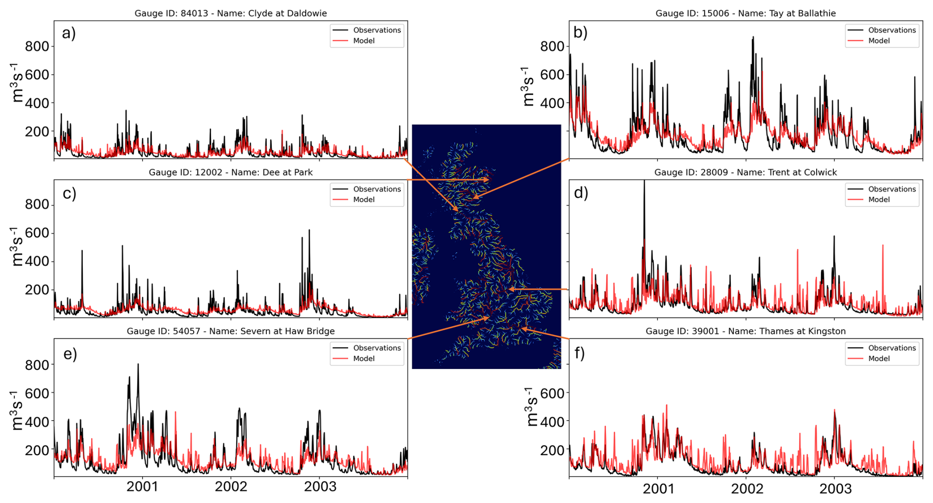
Figure 9 River discharge in the six catchments which have the largest river discharges of the United Kingdom, using the gauge closest to the sea (note this can still be > 50 km from the sea).

4 Introducing ensemble components

This section demonstrates the ensemble forecasting capability of RCS-UKC4, with a particular focus on waves, winds and ensemble spread of air temperature.

4.1 Quality of the ensemble wave forecast

We first analyse the quality of Significant wave Height (HS) and 10  m Wind Speed (WS) for a set of 5 d MO-ensemble forecasts (Table 2), including 4 named storm events associated with strong wind speeds: storm Larisa (10 March 2023), storm Poly (5 July 2023), storm Patricia (2 August 2023) and storm Betty (18 August 2023), one weak westerly case (10 July 2023) and one settled case (26 June 2023). The analysis focuses on day 3 of the forecast, as this is a critical period for using regional ensembles to provide guidance on hazards (Porson et al., 2020). We compare RCS-UKC4 ensemble simulations with the current operational Atlantic wave ensemble. The operational Atlantic wave ensemble is an uncoupled wave model (WWIII) that has a domain covering the whole Atlantic basin with a multi resolution cell structure allowing higher resolution over the UK (3 km). It is forced by winds from the current operational global atmosphere only ensemble MOGREPS-G (Valiente et al., 2023).

The spatial distribution of the observation buoys used for evaluating HS, WS, and SSTs are shown in Fig. 10. There is a clear concentration bias in HS and SST near the coast and oil rigs in the North Sea, while the WS measurements show a concentration bias primarily around the oil rigs in the North Sea. Coastal buoys around the UK were excluded from the wind speed analysis because their measurements over the time period considered were infrequent and unreliable.

Figure 10 Location of the buoys used for measuring HS (left), WS (centre), and SSTs (right) are shown. The figure presents the domain and locations of all the buoys used for each variable, marked with dots.

4.1.1 Wave Ensemble Forecast

When evaluating the reliability of an ensemble prediction system, the Root-Mean-Square Error (RMSE) of the ensemble mean is commonly compared to the average ensemble spread, calculated as the square root of the average ensemble variance (Fortin et al., 2014). Figures 11 and 12 include the bias, RMSE and ensemble spread of HS and WS for six cases. The RMSE excludes any observational error: we expect that a good ensemble has a spread to RMSE ratio slightly greater than one. RCS-UKC4 shows comparable skill for both HS and WS to the Atlantic operational wave ensemble. During storms, RCS-UKC4 often has improved bias for HS than the operational ensemble, with up to 90 % bias improvement for the Patricia case study (31 July 2023). The improvement is seen in the growing phase of wave development, though the decaying phase is relatively degraded in RCS-UKC4 by 20 %. During more settled weather conditions, RCS-UKC4 has generally reduced skill and overestimates HS, typically degrading the bias by about 20 %, but still improved relative to the operational ensemble.

Figure 11 Mean ensemble bias (dotted lines), RMSE (solid lines) and spread (dashed line) for significant wave height (HS) averaged across all buoys shown in Fig. 10. UKC4 performance is shown in yellow, standalone operational wave ensemble in grey. Each panel shows a 5 d forecast in spring and summer 2023, including 3 storms (top row, indicated with double arrows).

Figure 12 Same as Fig. 11 for wind speed (WS) using buoys shown in Fig. 10.

The improved RMSE in the coupled system may come from a combination of coupling, resolution and scientific configuration differences between the two systems. Nevertheless, this improvement possibly partly comes from the wind and wave modulation by tidal currents, which are particularly strong in the English Channel, Southern North Sea and Irish Sea, where most of the buoys are located. Tidal currents in NWS change direction every 6 h and typically reach about 1 m s⁻¹. Waves are amplified when they propagate against the current and dampened when they propagate in the same direction, resulting in the oscillations seen in the timeseries of a buoy in the English Channel (Fig. 13). Winds are also modulated by tidal currents (Renault and Marchesiello, 2022), which further modulates waves. Figure 13 demonstrates the benefit of coupling on forecasting HS in a tidally active area. RCS-UKC4 accurately represents the oscillations, particularly during and after the storm from 2 August 2023 to 5 August 2023. Tidal currents can amplify large waves during storms, as shown at 22:00 UTC on 2 August 2023, with a wave peak at 2.6 m, captured in the RCS-UKC4 ensemble spread. In contrast, the operational ensemble does not show any tidally induced oscillation, resulting in larger RMSE and poorer timing of the wave peak.

Figure 13 Impact of wave modulation by tidal currents in the English Channel. The regional coupled model (orange), Atlantic operational wave ensemble (grey) and observations (black), with the shaded area indicating one standard deviation around the ensemble mean. Left panel includes a background map data from OpenStreetMap (https://www.openstreetmap.org/copyright, last access: 8 September 2026).

Although there is initially no spread in HS for RCS-UKC4 as the ocean/wave initial condition in all members comes from the deterministic operational ocean-wave model, the RCS-UKC4 wave spread spins up to similar values to the operational ensemble in around 6 h (Fig. 11). After this, both models tend to be under-spread, with RCS-UKC4 being closer to a spread-to-error ratio of one than the operational system.

Figure 12 demonstrates that RCS-UKC4 tends to improve the wind bias by order ∼ 30 % through the 5 d forecast period, relative to the coarser resolution MOGREPS-G winds used to force the operational wave ensemble, with negligible improvements in the RMSE.

Density scatter plots of results across all ensemble members and all 6 cases examined highlight the representation of extremes in addition to more typically experienced conditions (Fig. 14). Both RCS-UKC4 and the operational wave ensembles are well centred around the 1–1-line, re-iterating their overall good quality. Both tend to overestimate HS below 2 m and underestimate for higher wave heights. Similar over/underestimation of WS is evident centred around 7.5 m s⁻¹. This is a common problem in wave and atmospheric models (Valiente et al., 2023; Wahle et al., 2017). This tendency is slightly exacerbated in the coupled ensemble, potentially because individual components within RCS-UKC4 are more finely tuned to run as uncoupled configurations.

Figure 14 Summary density scatter plots comparing the ensemble predictions against observations for all six cases across all buoys and all 5 d forecasts, covering the entire distribution of significant wave height (HS, a–b) and 10 m wind speed (WS, c–d). The plots include a red one-to-one line, a blue linear regression for HS below 2 m and WS below 10 m s⁻¹, and a green linear regression for HS above 2 m and WS above 10 m s⁻¹. The left column depicts the Atlantic operational wave ensemble, while the right column shows UKC4. Colorbar shows a fitted gaussian kernel density estimation.

4.1.2 Adjusting wind/wave coupling

The previous section showed improved wind biases in the RCS-UKC4 ensemble for the bulk of the distribution, though stronger underestimation of high WS compared to the global ensemble MOGREPS-G. However, wave improvements were mostly found for higher wave height and for the RMSE rather than biases. This suggests that RCS-UKC4 can be further improved in its wind/wave interactions. Three sensitivity tests have therefore been conducted:

• Increasing the coupling frequency from 1 h to 10 min

• Fine-tuning the wave growth parameter (Betamax)

• Converting the wind speed sent from the UM to WW3 model from 10 m winds to 10 m neutral winds, as WW3-ST4 is assuming a neutral wind profile to interpolate winds to the surface

The impact of these tests on HS and WS are analysed, with an additional focus on SSTs as a coupled system cannot afford to improve only one variable.

Impact of increasing the coupling frequency

Increasing the coupling frequency from 1 h to 10 min was intended to improve the diurnal cycle of SSTs and enable the representation and forecasting of meteotsunamis (Lewis et al., 2023; see also Sect. 5). Switching to 10 min coupling itself had no impact on the cost of the coupled system: exchanging fields more frequently does not increase the cost of the coupled system. However, the ocean timestep had to be reduced from 90 to 60 s, because more frequent coupling led to decreased ocean model stability, so the overall cost of the coupled system increased because the cost of the ocean component increased.

Increasing the coupling frequency to 10 min shifts HS, WS and SST increase and decrease forward in time (Fig. 15): by 1 h in waves, and 2 h for wind and SST. For waves, the forward lag is stronger when waves are growing, consistent with winds having stronger influence on growing waves, when waves extract kinetic energy from winds (Ardhuin et al., 2010; Janssen, 2004). This leads to marginal improvements in wave and wind forecasts, though can generate too early wave growth as on 2 August 2023 (Fig. 16). SST RMSE is consistently improved, particularly outside storm events, when a diurnal cycle develops. This is partly due to the correction in the delay introduced by coupling. where fluxes generated by one model are waiting until the next coupling time step to be sent to the other model. However, this would only explain 50 min differences in timing. The remaining difference is due to models adjusting to each other more frequently, being in closer equilibrium. Overall, increasing the coupling frequency improves SSTs and shows marginal improvements to wind and waves, and small deterioration in strong wave growth conditions.

Figure 15 Domain-averaged timeseries comparison of UKC4 with 1 h and 10 min coupling frequencies showing the mean HS (a), WS (b), and SST (c) across the entire UK domain for the storm Betty case study (16/08/2023). Coupling frequency: 1  (coupled_1h, yellow), and 10 min (coupled_10mn, green).

Figure 16 Three 5 d storm forecasts of 2023 spring and summer case studies, for HS (first row), WS (second row) and SST (third row). Comparing two different coupling frequencies; gold 1 h and green 10 min. The dotted lines represent the mean bias, and the solid line is the mean RMSE across all buoys through time. The black arrows indicate when the average WS across the whole domain exceeds 7.5 m s⁻¹.

Changing wind/wave coupling parameter (Betamax)

The wave growth parameter (Betamax) is a non-dimensional WWIII parameter that characterizes the maximum amount of energy exchanged between wind and waves. Four different Betamax parameters that were tested for 3 storm case studies: 1.6 (Bidlot, 2020), 1.48 (1.48 in Met Office regional deterministic system driven by the European Centre for Medium Range Weather Forecasting winds, Valiente et al., 2023), 1.39 (Met Office global Operational wave ensemble, Valiente et al., 2023) and 1.2 (Janssen, 1991). Overall, using a reduced Betamax decreased the mean bias across buoys for HS, with the opposite effect on WS and SSTs (not shown). Because the reduction from 1.48 to 1.39 was judged to be minor, and RCS-UKC4 typically shows a warm SST bias, the value was kept at 1.48. These sensitivity tests illustrated that a balance has to be reached in a coupled system, where a parameter cannot be tuned for a single variable (e.g. HS) without checking the impact on other variables (e.g. WS and SST).

Coupling Neutral Winds instead of Winds

When 10 m wind speeds are sent to the wave model, it calculates surface wind speed using a logarithmic profile assuming a neutral boundary layer profile. Therefore, sending neutral wind speed from the atmosphere to the wave model enables a more consistent treatment of momentum in the coupled system. Results indicated localised impacts during storm cases, generally resulting in improved skill (up to 60 % RMSE improvement for HS and 70 % for WS for storm Betty, but closer to 5 % improvements in other cases). Impacts on SST biases were of the order of 5 % and case-dependent, with no systematic change. These wind and wave changes appear to be case study dependent with storms being highly complex with a variety of different boundary layer stability depending on storm sectors. Given the improvements in most cases for HS and WS, and the more consistent treatment of momentum transfer between models, this change was adopted in RCS-UKC4.

Fine-tuning the wind/wave coupling in this paper was done on a few case studies and is limited by the sparse and irregular observation coverage. Future work will evaluate more wave properties against both satellite and in-situ wave buoy networks to provide a full assessment of wind and waves over long periods of time.

4.2 Impact of coupling on the atmospheric ensemble spread

For a good quality ensemble, the model error should be similar to model spread, so that the observations are contained within model spread. The 1.5 m air temperature biases can be substantial in atmospheric models: additional perturbations are applied to the sea surface temperature following Tennant and Beare (2014) to artificially enhance the spread in air temperature. These perturbations have a maximum amplitude of 2 °C and generate greater variations where the climatological day-to-day fluctuations in SST are largest. However, this perturbation strategy was designed for global prediction systems and subsequently adopted in the regional ensemble.

We investigated the impact of coupling on ensemble spread in air temperature when keeping these perturbations added to the SST field sent by the ocean to the atmosphere via the OASIS coupler. In a global coupled framework, Lea et al. (2022) found they could reduce the 2 °C maximum perturbation amplitude to 1.8 °C as coupling was able to provide a physically meaningful 0.2 °C spread. In RCS-UKC4 ensemble simulations, all the ocean and wave members are starting from the operational deterministic analysis of the ocean and wave models respectively. This is because regional ocean ensemble data assimilation is not yet mature enough to be included in the system, meaning that all spread generated in these components in coupled simulations are in response to the atmospheric spread in wind, and radiation.

Figure 17 shows the ratio of the standard deviation in surface temperature of RCS-UKC4 (coupled) and RAL3 (atmosphere-only) ensembles towards the end of the 5 d forecast (T + 112) for the different cases run over summer 2023 and winter 2023. Positive values (red shading) indicate regions with increased spread in the coupled ensemble relative to the uncoupled (atmosphere only) ensemble. When apparent, increased ensemble spread tends to be largest around UK coastlines, however there is substantial spatial variability linked to each case-specific situation. Enhanced spread is largest and most widespread during the 5 June 2023 and 19 June 2023 summer cases when marine heatwave conditions were dominant, and record shortwave radiative forcing was present (Berthou et al., 2024). In contrast, coupling has more limited impact on surface temperature spread in the winter, beyond local differences confined to near-coastal areas.

Figure 17 Map of standard deviation ratio between UKC4 (coupled) and RAL3 (atmosphere-land only) ensembles for surface temperature at T+112 of the forecast for the 12 cases run over summer 2023 and the 4 cases run over winter 2023. Greater than 1 (red colours) depicts regions where there is increased spread in UKC4 relative to RAL3. Less than 1 (blue colours) depicts regions where there is reduced spread in UKC4 relative to RAL3.

To understand the drivers of either relatively reduced or increased SST spread due to coupling, we investigate whether the SST anomalies imposed in the atmosphere-only run generate a flux adjustment in the radiative or turbulent heat fluxes, focusing on the largest sub-regions of the Northwest European shelf for visibility purposes (Wakelin_1, Wakelin_2, Wakelin_3, Wakelin_4, Wakelin_10 in Fig. 1b), results are still valid if more regions were included (not shown). Figure 18 shows the relationship between imposed SST anomaly and surface flux anomalies in each member for two summer atmosphere-only ensemble simulations, with spatially averaged results for five hydrodynamically-consistent ocean regions surrounding the UK (Fig. 1b). Results for shortwave radiation fluxes show large spread between members, but no relationship to the SST anomalies, indicating that this spread originates from atmospheric drivers linked with variations in cloud cover between members. In contrast, a negative relationship emerges for the long wave radiative fluxes, sensible heat flux, and particularly for latent heat flux. Warmer SSTs generate negative flux anomalies towards the ocean, which in a coupled system will act to cool it. In RCS-UKC4, where the SST will respond to changes in radiative fluxes, the latent heat flux (and to a lesser extent longwave radiative flux and sensible heat flux) response to SST perturbations will tend to dampen the SST anomalies, therefore acting to decrease the ensemble spread. Only increases in random shortwave perturbations are likely to increase SST spread. Therefore, the coupled ensemble spread in SST is more likely to increase when cloud cover variability between members and shortwave radiative forcing are large, while spread in SST is likely to decrease in cases dominated by latent heat flux cooling.

Figure 18 Scatter plots of flux anomalies (averaged over 5 d of the run) compared to SST anomalies (averaged over the last day) in the atmosphere-only ensemble. Top row is for the case initialised on 19 June 2023 and bottom row is the case initialised on 31 July 2023. First column shows SW heat flux anomaly, second column is LW heat flux anomaly, third column is sensible heat flux anomaly, and fourth column is latent heat flux anomaly. Each point is a member of the ensemble, and the different colours are a subset of Wakelin regions, as defined in Fig. 1b.

We now focus on explaining the difference in the magnitude of spread changes between cases, and in particular summer and winter. We show the relationship between net heat flux anomalies in the coupled system, versus SST anomaly growth or decay between UKC4 and RAL3 simulations in Fig. 19. In this figure, we added two additional sub-regions to investigate the behaviour of regions with different hydrodynamical properties. This relationship is usually positive, indicating that when a member has larger net fluxes into the ocean, the SST warms compare to the control, and vice-versa. However, the slope of the relationship varies between cases and regions: summer cases have a larger SST warming for similar flux differences, and the Irish sea, English Channel and southern North Sea (resp. Wakelin_9, Wakelin_4 and Wakelin_1) have smaller SST changes for similar flux differences compared to other regions. Figure 19 also indicates the average SST change which would be expected by a simple mixed layer heat budget computed on the averaged mixed layer depth over the 5 d and for each region. The mixed layer heat budget is calculated using surface flux anomalies integrated over 5 d, divided by the density of sea water, the heat capacity of sea water and the mixed layer depth averaged over 5 d. The mixed layer depth is obtained using (de Boyer Montégut et al., 2004) with a 0.2 °C temperature (density equivalent) gradient and 3 m reference level. Differences are consistent with the simulation results shown. Although a crude approximation therefore, the difference in mixed layer depth between winter and summer, between regions and cases largely explains the different SST response to flux differences. For example, the 19 June 2023 case has an extremely shallow mixed layer (∼ 11–12 m in the North Sea) and shows strongest changes in SST in the coupled system compared to atmosphere-only system. This is further supported by Wakelin_9 (Irish Sea) and Wakelin_1 (Southern North Sea) having steeper slopes than the other regions in the SST/flux relationship in summer (Fig. 19a, b). These areas are permanently mixed vertically, with an average 30 m depth, so that even large changes in flux result in small changes in SST in summer. The other areas of the shelf can develop a summer stratification, and therefore show a less steep slope, meaning small changes in fluxes can lead to larger changes in SST. In winter (Fig. 19c, d), when the mixed layer depth is deep (48 and 78–80 m in the central and northern North Sea respectively (Wakelin_2 and Wakelin_3), close to the average depth of these regions, any changes in fluxes arising from coupled feedbacks have very little effect on the SST.

Figure 19 Net heat flux anomaly in coupled simulations averaged over a subset of hydrodynamically consistent regions (Wakelin et al., 2012) defined in Fig. 1b versus SST anomaly difference between coupled and atmosphere-only simulations for each ensemble member. Each panel shows a different case: (a) and (b) are summer cases, (c) and (d) winter cases. SST anomaly is averaged over the last day, whereas net heat flux anomaly is averaged over the 5 d period. Solid lines indicate the average SST change computed using a simple mixed layer heat budget for each region.

In summary, RCS-UKC4 is likely to have increased air temperature spread relative to an atmosphere-only ensemble in summer cases with strong radiative fluxes and variability in cloud cover between members but is likely to decrease it in conditions dominated by strong winds and latent heat fluxes. Coupling is likely to have minimal impacts on spread in the winter.

5 Unlocking new high frequency sea surface height disturbance forecasts (meteotsunamis)

Finally, we explore new forecasting capabilities enabled by 10 min coupling between km-scale components. A tsunami is a series of waves caused by the displacement of water. The displacement may result from “bottom-up” seabed movement, such as that caused by earthquakes, landslides and volcanic eruptions or “top-down” movement, from pressure perturbations in the atmosphere. These “top-down” events are termed meteotsunamis (Makrygianni et al., 2026). Their period is between 2 and 120 min: they are therefore resolved by the ocean model rather than the wave model. They are generated by mesoscale atmospheric perturbations traveling offshore, such as squalls, gravitational waves, hurricanes and weather fronts. These changes are usually only of a few hPa over a few tens of minutes which corresponds to a few centimetres of sea level change, via a process known as the inverse barometric effect (Lewis et al., 2023). As the waves triggered by the perturbations travel towards the shore, they can be amplified by multi-resonant mechanisms that can drive their amplitude up to a meter. Such mechanics include (1) Proudman resonance, where the propagation speed of the air disturbance matches that of the wave $\sqrt{gh}$, where g is the gravitational acceleration and h is the water depth, (2) self-amplification, where a meteotsunami traveling towards the shore increases in amplitude due to the decrease in water depth, (3) basin or harbour resonance, where the meteotsunami frequency is close to the resonant frequency of the basin or harbour that is traveling through (4) Greenspan response, where the speed of pressure perturbation traveling along the coast is close to the resonant speed along-shore edges (Renzi et al., 2023).

In northwest Europe, meteotsunamis are less intense and frequent than in the US or the Adriatic Sea. Nevertheless, recent studies for the UK and Northwest Europe have shown that these events can cause significant disturbances and even be a high risk for coastal infrastructures, property and human life (Lewis et al., 2023; Renzi et al., 2023; Thompson et al., 2020; Williams et al., 2021). Lewis et al. (2023) produced a catalogue of events and showed their average frequency in the UK is around five per year, with one damaging event every five years. Currently, no early warning system is in place for this phenomenon in Northwest Europe.

The Environment Agency in the UK reported coastal floods on 31 October 2021 in the English Channel from Weymouth east to Portsmouth particularly Christchurch and Lymington. Impacts included flooding of quays, missed or late closure of tidal gates at Christchurch and Lymington. The Met Office operational surge forecast, forced with hourly global winds, did not indicate a surge near high tide, and no flood warning was issued. In this section, we investigate whether the km-scale coupled system with 10 min coupling frequency is able to represent and forecast this event, given its ability to explicitly resolve vertical motion in the atmosphere, its fine-scale bathymetry and coastline in a 1.5 km resolution ocean, and the possibility to exchange these fine-scale pressure perturbations every 10 min. RCS-UKC4 with 1 h coupling (UKC4-1h) is compared with RCS-UKC4 with 10 min coupling (UKC4-10min) to assess potential improvements in model performance relative to tide gauge observations.

5.1 Meteotsunami signal in sea surface height

To analyse the meteotsunami signal, we apply a high-pass Butterworth filter, a signal processing technique that attenuates low-frequency components while preserving high-frequency variations. Its calculation is:

$$\begin{array}{}\text{(1)}& H\left(s\right)={\displaystyle \frac{s^n}{s^n+{\mathit{\omega }}_{\mathrm{c}}^n}}\end{array}$$

where H(s) is the transfer function, s is the complex frequency variable, ω_c is the cutoff frequency, and n is the order of the filter. A 5th order high-pass Butterworth filter is used, with a 3 h cutoff for filtering both sea surface height (SSH) and mean sea level pressure (MSLP). These filtering parameters effectively remove low-frequency background variations while preserving the key high-frequency components of meteotsunami-related atmospheric and oceanic disturbances.

Observations from the Portsmouth tide gauge (black line in Fig. 20), where sea level is recorded every 15 minutes, indicate distinct positive anomalies on 31 October 2021 at 07:00, 09:30, 15:00 (Fig. 20a), more evident in the filtered time-series (Fig. 20b), where the peaks are seen with a 2.5 h frequency from 7:00 to 23:00. The 09:30 peak reached 24 cm amplitude and was responsible for the coastal floods reported by the Environment Agency. Simulations using the operational surge model (grey) and UKC4-1h (orange dashed line) largely reflect the lack of signal reported by the Environment Agency. While both models forecast some anomalies (up to 9 cm), they are too weak and occur around 12:00, after high tide. In contrast, UKC4-10min (orange solid line) produces a 7 cm change in sea level peaking at 08:45 during high tide, 15 cm at 09:45, 30 cm at 11:45, and further 10 cm oscillations until 23:00, with a 2 h frequency initially, which lengthens to 2.5 h in the afternoon.

Figure 20 (a) Raw output and (b) Butterworth high-pass filtered sea surface height for UKC4-10min (orange solid line), UKC4-1h (orange dashed line), operational surge model (grey line) and observations (black line) at Portsmouth tide gauge (cross in Fig. 21).

5.2 Atmospheric forcing

At the time of the event, a frontal system was moving across Ireland and the UK, ahead of a low-pressure system centred on Ireland at 06:00 on 31 October 2021 (Fig. 21a). It was associated with a band of heavy rainfall (> 8 mm h⁻¹) along the front (Fig. 21b). The dip in pressure is clearly seen in the 994 hPa isobar, on the coast of northern Brittany: a 50 km-wide pressure disturbance and of 1–1.5 hPa amplitude stretching from south-southwest to north-northeast across the English Channel (circled in Fig. 21). Convective activity within fronts is often responsible for strong, localised vertical wind speeds, and therefore, pressure disturbances of a few hPa.

Figure 21 Atmospheric conditions on 31 October 2021 at 06:00 UTC: (a) mean sea level pressure (hPa) and (b) hourly precipitation rate (mm h⁻¹). The oval shape highlights the region of pressure drop associated with the frontal rainband.

Sea surface pressure timeseries spaced 100 km apart across the English Channel (marked by stars in Fig. 22a) are shown in Fig. 22b. The frontal system is seen as a 1–1.5 hPa pressure drop in 30 min at 02:00 UTC on the western part of the Channel (blue), arriving at 08:30 just south of Portsmouth (red). This sudden pressure drop only lasts for 1 h: 1–1.5 hPa decrease for 30 min followed by 1–1.5 hPa increase for 30 min. UKC4-1h (dashed lines), although generally capturing the overall pressure tendency, clearly misses this 30 min pressure drop followed by 30 min pressure increase, as 1 h sampling frequency is too low to capture this short-lived pressure signal. This pressure disturbance associated with the front propagates with an estimated speed of 80 km h⁻¹. This closely matches the calculated phase speed of oceanic long waves in the English Channel, which is 60–90 km h⁻¹ (Fig. 22a). The alignment of these speeds suggests that the event was driven by Proudman resonance, although idealised experiments would be required to demonstrate this. Given the ocean model has 1.5 km resolution, this means that every 10 min, the pressure disturbance is re-applied 9 grid points further along. The front takes 6 h to travel from the blue to red point: the 1 hPa disturbance, generating 1 cm wave, is applied 36 times to the ocean, which is close to 30 cm generated by the model.

Figure 22 (a) Phase speed calculated as $\sqrt{gh}$, with g being acceleration of gravity and h the local bathymetry; (b) Timeseries of mean sea level pressure for the locations shown with stars on the phase speed map (a) (each colour is a different location); dashed line is hourly sampling, whereas solid line is 10 min sampling of mean sea level pressure.

The spatial representation of the signal is shown in Fig. 23. A low/high sea surface height (SSH) dipole emerges at the entrance of the Channel at 04:00. It propagates east, mostly visible along the UK coastline, at 06:00 and 09:00 the high SSH is near Portsmouth. It continues to propagate east at 10:15. At 12:00, the pressure disturbance is located in the southern North Sea, but the SSH signal is still visible, now with a positive signal in Northern France, negative signal in the middle of the Channel and positive signal in Portsmouth. This behaviour suggests the presence of seiching between the English and French coastlines, where oscillations become trapped within the Channel, where it is double the width of the perturbation (∼ 100 km), preventing immediate dispersion. Timeseries in two points confirm that the signal is anti-phased between the two coastlines (not shown). This explains that the anomaly persists in the afternoon of the 31 October 2021, after the frontal system has moved away.

Figure 23 Spatial Sea Surface Height Filtered for times before the event on 30 October 2021 during the event (04:00–12:00), and during its dissipation (18:00).

5.3 Forecasting a meteotsunami with the RCS-UKC4 ensemble forecast

To assess the ability of RCS-UKC4 to forecast meteotsunami events, we performed ensemble simulations with lead times of one and three days. The filtered SSH for the 1 d forecast simulations is shown in Fig. 24. In the one-day forecast, roughly six ensemble members successfully captured the meteotsunami throughout its full duration, predicting a signal of approximately 0.3 m. The ensemble shows the likelihood of an anomaly around the time of high tide (when the observed signal is maximal). This reflects a relatively high level of accuracy at short lead times. In the three-day forecast (not shown), three ensemble members were still able to clearly reproduce the event, demonstrating the model's potential to deliver useful early warnings even several days ahead.

Figure 24 Meteotsunami ensemble forecast of filtered sea surface height (m) for Portsmouth location started 24 h before the event. Each orange line is an ensemble member, and the black line is the observations.

6 Conclusions and perspectives

We present an updated version of the Regional Coupled System – UK Coupled domain version four (RCS-UKC4). Developments to the Regional Coupled Suite workflow used to configure and run RCS-UKC4 provide flexibility to couple different components of the system in several ways, and a diversity of modes for running experiments. This includes demonstrations in this paper of new capability to run climate simulations and near-real-time ensembles, in addition to the previously supported deterministic case-study or longer hindcast modes. The river routing component has been substantially developed and improved. A new marine biogeochemistry component has also been added, as discussed in depth by Partridge et al. (2026). This paper documents the development from individual model code and configuration updates to a final coupled configuration. This journey requires pragmatic compromises, as a one solution-fits-all is difficult to attain in coupled modelling. RCS-UKC4 includes several changes to coupling science choices, including to ocean light penetration parameters, coupling exchanges between atmosphere and waves, coupling frequency (with impact on ocean model timestep). Attempts to tune the wave growth parameter indicated keeping the UKC3 value balances optimal performance across wind, waves and SST.

Changing the regional atmosphere model configuration in RCS-UKC4 had a large impact on heat budget reaching the ocean, and in particular the radiative terms. RAL3.3 has sufficient quality of surface fluxes over the ocean that multi-year simulations with RCS-UKC4 maintains domain-average seasonal SST bias of within 0.25 °C, locally up to 1.5 °C. Importantly, the SST does not drift from one year to another, indicating a balanced coupled system. Development of RCS-UKC4 has included assessment and enhancement to the representation of rivers in regional Met Office configurations, with reasonable geographic and temporal representation of broad-scale characteristics. Nevertheless, day-to-day streamflow variability tends to be underestimated in the west and north of the UK and overestimated in southeast UK. Weedon et al. (2023) recommend a change to saturated hydraulic conductivity in the soils to take into account bedrock properties, which will be a topic of research for the next coupled version.

Assessment of RCS-UKC4 ensemble forecasts shows improved skill for ensemble wind and wave forecasting around the UK relative to its uncoupled model components, with better performance during storm events and in shallow regions where tidal energy dissipates through strong tidal currents. Nevertheless, it tends to underestimate extreme wind and waves and overestimate weak waves, although this is a common bias among models. This suggests that further improvements to the representation of boundary layer momentum mixing in high wind regimes is necessary for the next version of the regional coupled model. The effects of coupling on winds are reduced in RCS-UKC4 compared to UKC3, as the drag parameterisation in the new atmosphere and land configuration RAL3.3 is now closer to the WAVEWATCH III ST4 parameterisation. Compared to atmosphere-only simulations, coupling to a wave model reduces moderate wind speed and increases extratropical storm wind speeds, it also produces a larger variety of drag coefficients for a given wind speed, increasing spread around the drag/wind relationship. We also showed that a coupled system will tend to decrease the ensemble spread through negative SST/turbulent flux feedback, except in cases with a shallow mixed layer, where any changes in radiative fluxes between members (due to large-scale differences or perturbed parameters) can introduce large spread in the coupled system, independently from the SST perturbations imposed on the atmosphere.

Finally, coupled regional ensemble forecasts together with 10 min coupling frequency offer promises for early-warning system for meteotsunami hazards. We demonstrated that RCS-UKC4 can represent and forecast a relatively simple case of meteotsunami, which caused flooding on the southern coast of the UK. This event was very poorly captured in the current operational surge model. Makrygianni et al. (2026) explore a more complex meteotsunami case, also showing forecasting skills and fully explaining its complex atmospheric origin.

In summary, RCS-UKC4 has evolved to be a mature coupled modelling framework, suitable as a basis to provide future enhanced operational weather prediction and production regional climate capabilities. The Met Office has now integrated coupled experiments early in the development cycle of its Regional Atmosphere and Land configurations, which adds a constraint of good quality of RAL at the ocean surface (Bush et al., 2025) and good quality of the land for river flow. The regional coupled system has also been demonstrated to be used to generate plausible climate simulations, and to help process-understanding complex compound phenomena such as marine heatwaves and their regional feedback on the atmosphere and land (Berthou et al., 2024), including during hazardous multi-hazard coastal events (Goswami et al., 2026). Developments described here also underpin application of RCS to different regional domains of interest worldwide by Momentum Partners, with further work to assess the sensitivity tests carried in this study over tropical domains (Castillo et al., 2022; Thompson et al., 2021).

Future research will further assess the quality of RCS-UKC4 for multi-hazard forecasts and projections, will quantify the impacts of a km-scale regional coupled on regional climate change signal and will help quantify the current and future meteotsunami risks. The integration of biogeochemistry has already furthered our understanding of compound physical and biogeochemical events, such as waves, marine heatwaves and phytoplankton bloom interactions (Partridge et al., 2026). Developments of wind farm parameterisations in the system will also enable to inform climate change mitigation strategies by helping the planning of offshore wind farm development. Finally, long simulations with a high-quality regional coupled system will enable training machine learning models across multi-components of the earth system.