The Geoengineering Model Intercomparison Project (GeoMIP) contribution to CMIP7 – description of new experimental protocols and preliminary results

The Geoengineering Model Intercomparison Project (GeoMIP) is a coordinated international model intercomparison effort with the aim of providing robust experimental protocols for simulations of various Solar Radiation Modification (SRM) methods. Through many iterations and discussions within the GeoMIP community, it has become clear that balancing simplicity, scientific realism, policy relevance and associated complexities is fundamental when designing modeling experiments. Such experiments must both diagnose areas of model agreement and disagreement through the lens of climate science and provide results useful for understanding the potential downstream impacts of SRM across different sectors. Here we present a suite of new climate model experiments designed for the Coupled Model Intercomparison Project Phase 7 (CMIP7), building on lessons learned from previous GeoMIP experiments, recent SRM research, and new simulations developed for CMIP7. We provide detailed experimental designs and their underlying rationale, including preliminary results from sensitivity analyses performed with CMIP6 models. Compared to previous GeoMIP iterations, we organize experiments into three categories: (i) Preparatory Experiments, designed to diagnose model responses and inform more complex experimental designs; (ii) Tier 1 experiments, the core simulations that all participating models should run; and (iii) Tier 2 experiments, which provide a flexible framework for exploring structural and scenario uncertainties under SRM, including the potential interaction with temporary overshoot scenarios and tipping elements dynamics. This framework encourages modeling groups to propose their own experiments building upon the Tier 1 backbone, enabling more targeted exploration while ensuring cross-model compatibility.

1 Introduction

Solar Radiation Modification (SRM, also known as solar geoengineering or climate intervention) encompasses a broad category of theoretical methods that aim to affect Earth's energy balance with the goal of potentially reducing the impacts of anthropogenic global warming. Many of these methods are based on real-world analogues that suggest such interventions could be effective, either regionally or globally.

Stratospheric Aerosol Injection (SAI) is inspired by observations of large explosive volcanic eruptions, such as Mt. Pinatubo in 1991, in which sulfate aerosols or their precursors are injected in the stratosphere, reflecting a portion of incoming sunlight before it reaches the troposphere and thereby cooling the planet. Marine Cloud Brightening (MCB) is inspired by observations of increased cloud albedo due to aerosol shipping emissions and lower-atmospheric injections of sulfate from some volcanic eruptions, leading to an increase of Earth's albedo through increased cloud brightness and other cloud changes such as changes in cloud coverage. Proposals for Cirrus Cloud Thinning (CCT) or Mixed-phase Cloud Thinning (MCT) arise from observations of the warming impact of tropospheric ice clouds, and questions whether their coverage could be reduced in order to allow for more terrestrial radiation to escape to space.

The known natural events that inspire these proposals suggest they could be replicated artificially, though with obvious engineering challenges (Smith, 2024). However, a broad understanding of the basic physical principles behind such analogues does not necessarily provide a deeper understanding of how effective these methods could be in the real world; both in terms of their actual capacity to reduce surface temperatures and of the downstream ramifications of a given cooling source. Both issues can be investigated through the use of climate models of different complexities, from simpler Energy Balance Models (EBMs) to highly complex Earth System Models (ESMs). Over the last 25 years of research within this field, such climate models have shown that none of those methods can simply “turn back the clock” (Visioni et al., 2021b), reverting the climate to the same state that it was in before temperatures rose due to rising greenhouse gases. Models differ across various components of the projected response to SRM (Haywood et al., 2025) and in their assessment of the methods' efficacy, due to a combination of model structural differences, parametric uncertainty, and different assumptions in how perturbations are represented as well as lack of inclusion of certain key underlying physical, chemical or natural processes in the models (Eastham et al., 2025). Nevertheless, they have also shown that in scenarios in which further warming is prevented through SRM in more or less idealized ways, and in which the cooling is maintained over time and is somewhat uniform in nature, key climatic risks could be reduced (Irvine et al., 2019; Tye et al., 2022; Wells and Haywood, 2025), albeit not always uniformly geographically (Feng et al., 2025; Egbebiyi et al., 2025). Additionally, research has identified non-negligible secondary impacts or “unintended consequences” arising from the application of such methods, for instance on atmospheric composition (Tilmes et al., 2022; Bednarz et al., 2025b). It is important to acknowledge the limitations of preliminary assessments on various fronts. Firstly, on the scenario front, the assessment of uniform, constant deployment may neglect considerations of irregularities in the potential deployment over time (Trisos et al., 2018) or of potential asymmetries in deployment across hemispheres (Haywood et al., 2023). Secondly, on the modeling front, many of these assessments may over-rely on one or few models, under-representing uncertainties (Henry et al., 2023), or the models may lack the spatial resolution necessary to correctly capture regional dynamics (Sun et al., 2026b), or key processes altogether, for instance in the ecological sphere (Zarnetske et al., 2021). These known limitations reinforce the importance of a systematic approach to coordinating modeling efforts.

The Geoengineering Model Intercomparison Project (GeoMIP) is a coordinated, international effort with the aim of providing robust experimental protocols for Earth system model (ESM) simulations of various SRM methods. This coordination has three main identifiable goals: (1) enabling a better understanding of inter-model differences in SRM simulations, by ensuring experimental protocols are as detailed and well documented as possible to reduce potential divergence arising from differences in the modeling set-up; (2) offering a standardized framework of simulations for the purpose of broader assessments of SRM, making sure decisions around experimental details are taken by a broad representative community of climate scientists, which includes modelers and those interested in potential downstream impacts of SRM (including on agriculture, society, infrastructure and ecological systems) that is capable of assessing and documenting different needs and opinions; (3) supporting the community of users by facilitating data sharing practices and coordinating analyses. GeoMIP facilitates this coordination by organizing annual workshops, where researchers can both present their recent findings and discuss future steps, and for which reports are publicly made available every year (see, for instance, Visioni et al., 2025 for the meeting held in 2025 where many of the decisions reported in this document were taken), as well as by coordinating with the broader Climate Model Intercomparison Project (CMIP) and World Climate Research Program (WCRP) community to ensure relevance and compliance with best practices, for instance informing efforts to better coordinate data requests for the most important variables for analyses (Juckes et al., 2025).

A review of GeoMIP's role and efforts over the years, including a detailed list of experiments performed by the community, as well as lessons learned by previous experiments, was provided in Visioni et al. (2023c). Since then, the community has continued discussions around future experiments to run as part of phase 7 of CMIP (CMIP7), considering both recent advances in understanding the design space of different SRM techniques and models' development (such as the potential inclusion of an interactive carbon cycle in CMIP7 models) as well as changes in other MIPs of relevance (for instance, the Scenario Model Intercomparison Project, ScenarioMIP). In particular, in Visioni et al. (2024) a new, intermediate experimental protocol was proposed, noting that the original CMIP6 protocol described in Kravitz et al. (2015) required some updates that would have enabled continued policy relevance and connection to other MIPs on the scenario side as well as updating the potential intervention strategies to be simulated based on the most recent research. As an example, the original G6sulfur experiment simulated initialization of SRM in 2020 and simulated the intervention under the Shared Socioeconomic Pathway (SSP) scenario 5-8.5, whose relevance and plausibility has been hotly contested (Burgess et al., 2020; Schwalm et al., 2020).

In this paper, we describe the set of experiments decided by the GeoMIP community for CMIP7, detailing both the underlying reasoning behind the specific decisions as well as providing as much guidance as possible for modeling teams. We describe first what we call the “Preparatory experiments” in Sect. 2, which are shorter, more technical idealized simulations to enable the design of the main CMIP7 simulations, traditionally termed “Tier 1”, which are described in Sect. 3; followed by a description of a broader range of experiments termed “Tier 2” that both aim to expand the range of potential scenarios under analyses as well as allowing for some more tentative experiments, in Sect. 4.4. Experiments described here include SAI, MCB and MCT. An idealized experiment involving CCT was proposed in Kravitz et al. (2015) (G7cirrus) but its results from four ESMs were only recently analysed in Smith et al. (2026), and the community has not expressed specific interest in updating this experiment or proposing new ones for CMIP7; this doesn't preclude that renewed interest might result in future GeoMIP CCT experiments.

2 Preparatory experiments

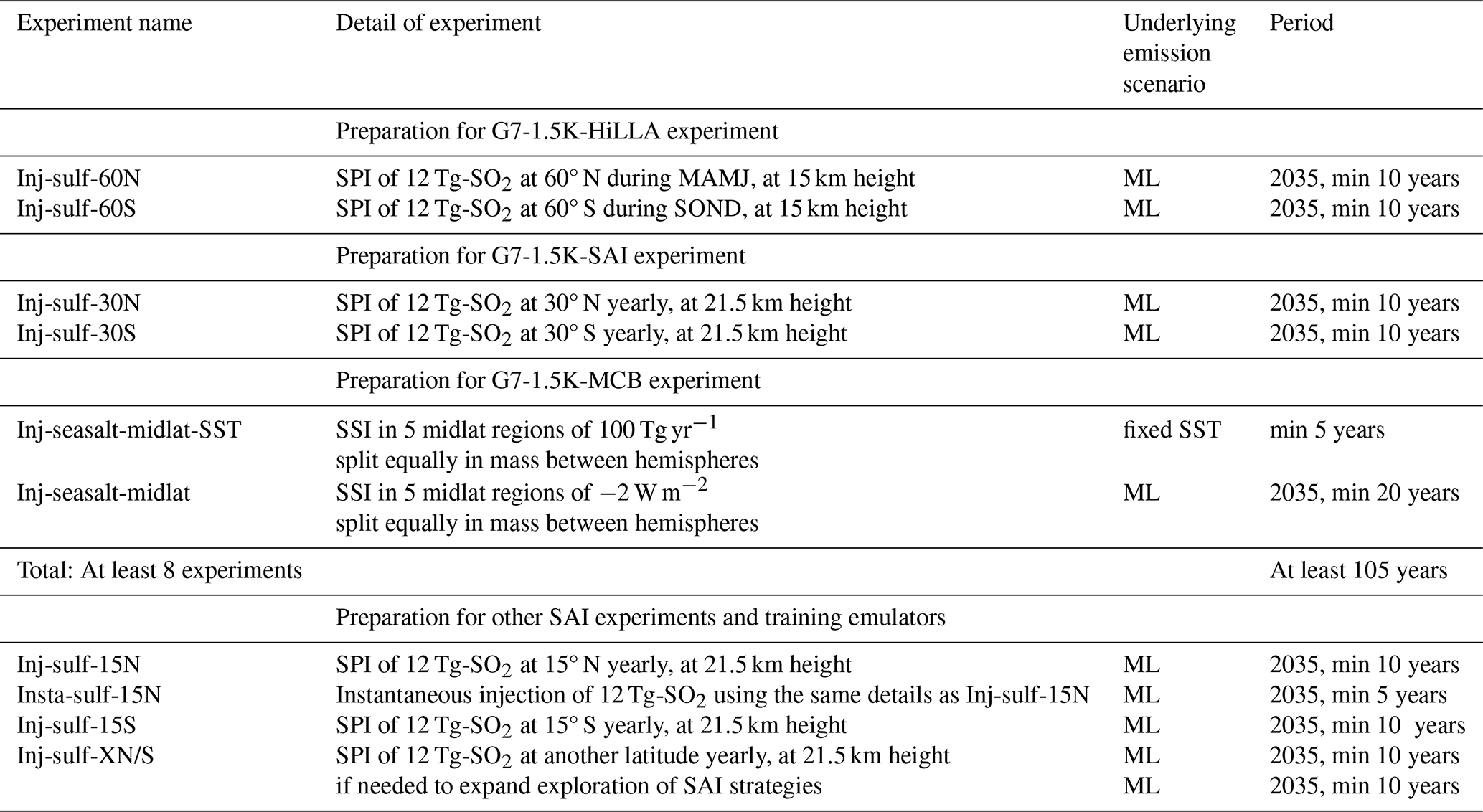
Before running the main Tier 1 experiments, modeling teams are advised to run these simpler, shorter experiments that allow for a better diagnosis of the models' responses to the Tier 1 experiments, as well as clarifying the models' sensitivities to the interventions. Consistently defined preparatory experiments serve to both enable clearer assessment of process differences across models and provide a template to simplify the preparation for the Tier 1 simulations based on past modeling experience. A detailed explanation of all these experiments, listed in Table 1, is provided in the following subsections.

Table 1 Process understanding, preparatory experiments to help run and interpret the Tier 1 experiments. SPI = Single Point Injections; MAMJ = March, April, May, June; SOND = September, October, November, December; SSI = Sea salt injections, values refer to the injection rate of NaCl which is typically around 3.5 % in sea-water; SST = sea surface temperature; ML = Medium-Low scenario. The last row shows the total number of experiments and the minimum number of years of simulation (one ensemble member is sufficient).

2.1 Single point injection location SAI simulations

Modeling centers aiming to run the G7-1.5K-SAI (and similar) simulations should consider performing single point injection (SPI) simulations of 12 Tg-SO₂ for a number of years (10 years is the minimum, 35 years is suggested) at specific latitudes, using the same fully-coupled atmosphere-ocean configuration as the one they plan to use for G7-1.5K-SAI. SPIs at 30° N, 15° N, 15° S, 30° S were already proposed as a testbed experiment in CMIP6 in Visioni et al. (2023a) in order to understand models' sensitivities to different injection locations and to allow for the calculations necessary to devise the feedback controller (MacMartin et al., 2017). These simulations have been shown to be very informative in diagnosing models' responses to SAI, for instance helping understand how the evolution of the aerosol plume affects the Atlantic Meridional Overturning Circulation (AMOC) or Arctic sea ice (Bednarz et al., 2025a; Kim et al., 2025), as well as to train climate emulators capable of better spanning the space of SAI strategies (Farley et al., 2026). For CMIP7, the set has been expanded to include injections at 60° N and 60° S for the High Latitude, Low Altitude (HiLLA) simulations, and given earlier results from Lee et al. (2023) and Duffey et al. (2025) at an altitude of 15 km, whereas injections at 30° N and 30° S should be performed at an altitude of 21.5 km as described in Richter et al. (2022). The injection longitude is not as important for injections significantly above the tropopause (Sun et al., 2023), but for consistency injections should be all at 0° E.

To be most useful, modeling teams running this set of preparatory experiments should also include diagnostics that help evaluate how injection location shapes regional climate systems. This could include variables that enable the evaluation of changes in monsoon rainfall (daily precipitation, sea surface temperatures), Arctic sea ice (extent and volume), and the AMOC (through ocean circulation diagnostics), as well as variables that enable estimates of hydrological cycle changes (see for instance the analyses of freshwater availability in Rezaei et al., 2026). Such diagnostics can help identify model dependent sensitivities and clarify the extent to which injection strategies can minimize disruptions while achieving the desired cooling target. Preparatory experiments also provide an opportunity to test the robustness of SRM strategies across diverse climate models. By systematically analysing responses across regions, they ensure that future SRM assessments can incorporate perspectives from different climates and socio-economic contexts, rather than focusing only on global averages. This broader approach strengthens the scientific foundation of Tier 1 experiments and enhances their relevance for both science and policy. SPI simulations have shown great promise as training elements for SAI climate emulators (Farley et al., 2026), and extending the number of models providing SPI simulations at different latitudes could provide further training data to improve and expand the exploration of different scenarios beyond what is feasible to do with ESMs.

Modeling centers should also consider running a version of the 15° N case (Inj-sulf-15N) with the same yearly amount (12 Tg-SO₂), location and height (21.5 km), but where the injection is instantaneous, on January 1st, in order to also provide a comparison of pulse versus continued injection impacts (Plazzotta et al., 2018), and that could provide a point of comparison with volcanic-related MIPs such as VolMIP (Zanchettin et al., 2022) and ISAMIP (Quaglia et al., 2023). Additionally, it is worth noting here that, as part of the Detection and Attribution MIP (DAMIP, Gillett et al., 2025), there are CMIP7 experiments aimed at isolating the historical volcanic forcing (hist-volc), and that CMIP7 forcings will also include volcanic SO₂ emissions (Aubry et al., 2026): the use of these simulations could be rather important to evaluate the SAI response in models in light of their response to historical volcanism.

2.2 Midlatitude MCB benchmarking simulations

MCB simulations for GeoMIP7 focus on a strategy in which MCB accumulation-mode sea salt aerosol emissions are emitted at the ocean surface in five mid-latitude ocean regions, with emission rates set to produce equal areal-sum emissions in each hemisphere, following recent testbed simulations (Hirasawa et al., 2026b, a) (see discussion and region definitions in Sect. 3.4). To prepare for the G7-1.5K-MCB scenario simulations, modelers should conduct two benchmarking simulations aimed at characterizing the cloud susceptibility and climate response to mid-latitude MCB: Inj-seasalt-midlat-SST and Inj-seasalt-midlat. This two-stage approach is motivated by model intercomparison work showing large differences in the aerosol-cloud forcing susceptibility to MCB sea salt aerosol emissions (Stjern et al., 2018; Rasch et al., 2024) due to differences in the size distribution of aerosol emissions and aerosol-cloud process uncertainty. Thus, in contrast to the SAI preparatory simulations, we request that modelers first estimate the effective radiative forcing from MCB using a fixed sea surface temperatures simulation (Inj-seasalt-midlat-SST). This simulation should use present-day SST and emission fields if possible and we recommend an initial emission rate of 100 Tg yr⁻¹ of NaCl (see below for the recommended aerosol size distribution) at the lowest atmospheric level. This falls roughly within the emission rates found in Alterskjaer et al. (2013) and Hirasawa et al. (2026b). In addition to easing the benchmarking process, consistently defined fixed SST simulations will be necessary for conducting process analysis studies to understand aerosol, cloud, and other processes that cause inter-model differences in MCB efficacy that are crucial for improving process understanding, identifying model deficiencies, and constraining the potential forcing from MCB.

The magnitude of MCB forcing depends strongly on the details of the injected sea salt aerosols, particularly the size distribution of the emitted aerosol as the aerosol-cloud interactions depend primarily on the aerosol number flux rather than the mass flux (Rasch et al., 2024). Previous ESM and parcel modeling work has identified accumulation mode aerosol as the most effective size to achieve cloud brightening (Alterskjær and Kristjánsson, 2013; Connolly et al., 2014; Wood, 2021) with approximate effective dry radii of 30 to 50 nm, depending on the activation parameterization. We recommend modelers use injected sea salt emissions in this size range, though we recognize this may not be strictly possible depending on sea salt emission parameterization implementation. MCB scenario simulations have been successfully completed with sea salt aerosol effective radii of up to 180 nm. However, emission size can drive large variations in the sea salt aerosol mass required across the models (Hirasawa et al., 2026a, Fig. 4a), meaning careful documentation of the emitted sea salt size distribution is necessary to compare models' responses, as the inter-model range tends to decrease when considering the number flux instead (Fig. 4b). This documentation should include the assumed dry aerosol size distribution (mode radius and geometric standard deviation, or bin/mode boundaries for sectional schemes) and the assumed particle density.

Using the information from this simulation, modelers should then conduct a coupled simulation to estimate the climate response sensitivity to MCB (Inj-seasalt-midlat). This simulation is patterned on previous GeoMIP MCB simulations, G4cdnc and G4sea-salt (Kravitz et al., 2013; Ahlm et al., 2017), with a Medium-Low (ML) emission scenario as a reference case and a time-constant MCB emission rate applied for a minimum of 20 years starting in 2035. In contrast to previous simulations, we prescribe a target forcing (−2 W m⁻²), rather than a predetermined emission rate or droplet number enhancement. The MCB aerosol-cloud forcing is non-linear, however a linear assumption is likely sufficient to provide a reasonable estimate of the climate sensitivity. Thus, we recommend setting the emission rate to 100 Tg yr${}^{-\mathrm{1}}\times (-\mathrm{2}$ W m${}^{-\mathrm{2}}/$ ERF_100 Tg), where ERF_100 Tg is the effective radiative forcing computed from Inj-seasalt-midlat-SST. The temperature response derived from this simulation will then enable modelers to design and conduct the G7-1.5K-MCB simulations.

3 Tier 1 CMIP7 experiments

The Tier 1 experiments are higher-priority fully coupled experiments that all modeling teams are encouraged to run. The underlying framework behind the scenario choices has been explained in detail in Visioni et al. (2024) for the experiment G6-1.5K-SAI. Visioni et al. (2024) was meant to both collect the thoughts and opinions of the GeoMIP community about what constitutes a broadly agreed upon, policy-relevant SRM experiment and to devise an experiment that could be run with some consistency with CMIP6 models and with CMIP7 models, in order to compare more easily across models' generations. This meant avoiding too high GHG emission scenarios that might not have a CMIP7 counterpart, as well as being considered less realistic, and selecting a scenario that was more consistent with current and near-term future emission trajectories: for CMIP6, that entailed selecting SSP2-4.5 (Burgess et al., 2020), whereas during the Fifteenth GeoMIP workshop (Visioni et al., 2025) the ML scenario was selected as the CMIP7 counterpart. During the Fifteenth and Sixteenth GeoMIP workshops, there was extended and lively debate over the selection of the ML scenario over the M one: while neither are entirely compatible with SSP2-4.5, ML is certainly on the more “optimistic” side, with emission reductions starting sooner and far more extensively as compared to M, where emissions plateau throughout the century. While full consensus was elusive, a clear majority of participants preferred ML on the specific ground that simulating SRM methods under an emission scenario with strong mitigation would strengthen the message that SRM should not be considered as a substitute to mitigation, and that a stronger physical signal due to more cooling could be obtained by simulating a scenario with like G7-0.5K-SAI (see Sect. 4.4).

This also meant anchoring the SRM target to a clearly defined metric that could be consistent between simulations with concentration-driven CO₂ and simulations with emission-driven CO₂. For this reason, the goal of the Tier 1 CMIP7 simulations, just like the CMIP6 ones, is to deploy SRM to maintain global mean temperatures at 1.5 °C above Preindustrial (i.e. a time period as close to “present day” as possible). The definition of 1.5 °C above Preindustrial (PI) is somewhat different from what is usually used: after testing and analyses, it was decided to anchor the definition of 1.5 °C above PI for the purpose of the simulations' target to each model's average global mean surface air temperatures (GMSAT) in the period 2020–2039. This rationale has been explored in Visioni et al. (2024); mainly, models' actual PI temperatures diverge greatly, and so does the period 1850–1900, which is usually used as a reference timeframe in the IPCC and other assessments. On the other hand, anchoring the target to the actual models' near-present time temperatures allows for models to have a consistent start date for the SRM deployment, as well as making it easier to compare across models with different base states, and across model generations.

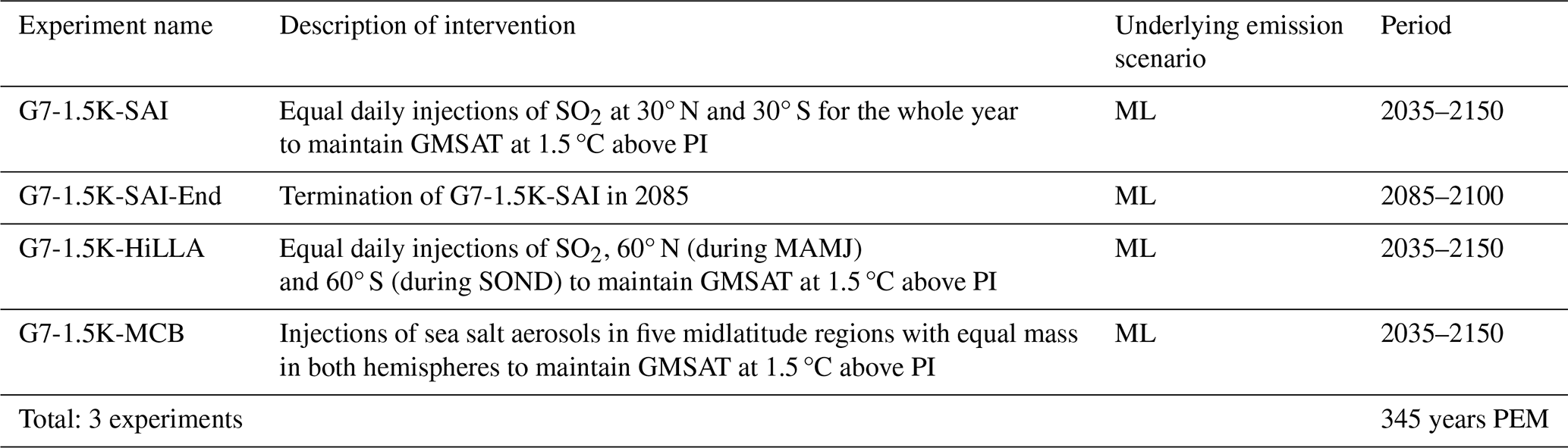
Table 2 lists the four experiments proposed as Tier 1, together with a brief description of the intervention, that will be expanded upon in the following subsections, and details about the underlying scenario used (van Vuuren et al., 2025) and the time period in which the simulations should be run.

In terms of nomenclature, we have decided to use the G6 moniker (i.e. G6-1.5K-SAI) for simulations run with CMIP6 models and scenarios, whereas the G7 moniker (i.e. G7-1.5K-SAI) is used for simulations run with CMIP7 models and scenarios. The differences and similarities between the two scenarios are sketched in Fig. 1. For each experiment, 3 ensemble members are suggested. Considering the CMIP7 scenarios will have extensions to 2150, it will be preferable if at least one ensemble member can be extended to 2150, whereas the others are only run to 2100.

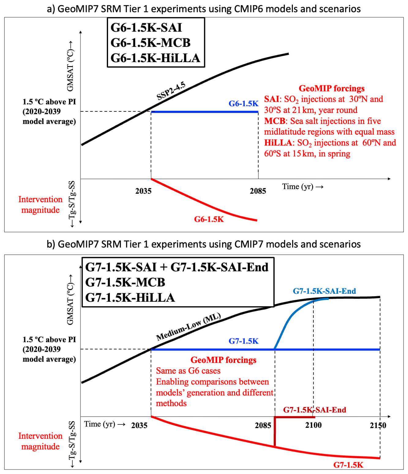
Figure 1 Schematics of G6 and G7 Tier 1 experiments, with differences between underlying scenarios from CMIP6 and CMIP7 sketched and details about the forcing methodologies (consistent across G6 and G7). The black lines represent the ScenarioMIP scenarios selected as a background for the experiments; the blue lines represent the related GeoMIP experiment; the red line in the bottom part of the plots represents the intervention magnitude (depending on the specific experiment, measured in Tg-S or Tg-SS (sea salt)).

Table 2 Tier 1 experiments for GeoMIP7. Specific details about the experimental set-ups and their justifications are provided in the text; Determination of injection amounts in the experiments to be performed through a 1 Degrees-of-freedom (DOF) feedback controller as discussed in Kravitz et al. (2016); Lee et al. (2025a). GMSAT = Global Mean Surface Air Temperature; SAI = Stratospheric Aerosol Injection; HiLLA = High Latitude, Low Altitude; MCB = Marine Cloud Brightening; ML = Medium-Low scenario (van Vuuren et al., 2025); PEM = Per Ensemble Member.

3.1 G7-1.5K-SAI

The G7-1.5K-SAI experiment is functionally identical to the G6-1.5K-SAI experiment, but uses a CMIP7 emissions scenario. In G7-1.5K-SAI, hemispherically symmetric SAI in the subtropical stratosphere is used to maintain a fixed GMSAT of approximately 1.5 °C above the preindustrial average. The experiment branches from the ML emissions scenario, begins in model year 2035 and runs until model year 2150. Given how we've defined 1.5 K above preindustrial, this means the start in 2035 in all models does not require a large initial amount of SO₂ to be injected all at once, as it happened in the ARISE protocols for UKESM (Henry et al., 2023). Each year, SO₂ is injected into the stratosphere in sufficient quantity to cool the planet by the amount needed to maintain the prescribed temperature target. The total quantity of SO₂ is placed into grid boxes at 21.5 km altitude as per the Inj-sulf-30N/S simulations above, divided evenly between 30° N and 30° S latitude.

3.1.1 Why symmetrical injections?

As discussed in Visioni et al. (2024), the one-degree-of-freedom (1-DOF) injection strategy used in the G6- and G7-1.5K-SAI experiments is intended to balance optimality, plausibility, and simplicity. By using a 1-DOF strategy, we aim only to maintain GMSAT at 1.5 K, but more complexity (e.g., aiming to also manage regional impacts or large-scale gradients) is possible. Previous research into the optimization of SAI strategy design has identified (at minimum) two more degrees of freedom in the surface temperature response (Lee et al., 2020). Firstly, an imbalance in radiative forcing between the Northern and Southern Hemispheres will push the Intertropical Convergence Zone (ITCZ) towards the warmer hemisphere; this means that single-hemisphere injection is generally considered to be undesirable (Haywood et al., 2013), and SAI simulations are usually hemispherically symmetric or strategically managed across hemispheres to maintain the interhemispheric temperature gradient. Secondly, the latitude(s) of injection determine the relative amount of cooling at the tropics vs. the poles; as such, over the past decade, strategy design has gravitated towards off-equatorial (rather than equatorial) injection to offset polar amplification and avoid overcooling the tropics and undercooling the poles. SAI simulations have been conducted which simultaneously manage, or attempt to manage, all three simultaneously (henceforth, a “3-DOF strategy”) with injections at multiple latitudes simultaneously, usually 15 and 30° N and S. However, the optimal injection strategy, or even the ideal set of injection latitudes across which to optimize, is unique to different climate models (Henry et al., 2023). To maintain simplicity, for G6-1.5K-SAI and G7-1.5K-SAI, we instead choose a 1-DOF design (i.e., maintain GMSAT only) and choose an injection strategy likely to minimize disruption of the other two degrees of freedom. Figure 2, taken directly from Lee et al. (2026b), compares temperature changes for G6-1.5K-SAI and G6sulfur; both are 1-DOF strategies, but G6-1.5K-SAI (30° injection) has less residual warming at the poles and over NH land, on average, than G6sulfur (equatorial injection). G6-1.5K-SAI also disrupts tropical precipitation over land significantly less than G6sulfur (see Lee et al., 2026b, Fig. 8). Hemispherically symmetrical 30°  is unlikely to be the “ideal” injection strategy for any of the participating models (and, indeed, is known not to be for most of them), but based on the G6-1.5K-SAI results, we know it is a reasonable choice for a 1-DOF strategy which will cool the planet while cooling the poles and limiting ITCZ disruption more effectively than equatorial injection. Additionally, analysing how well (or poorly) the strategy achieves these secondary objectives for individual models will provide insights into how injection strategies might be improved in each model. For example, G6-1.5K-SAI overcools the Northern Hemisphere (NH) in the CESM2 model, suggesting that Southern Hemisphere (SH) injection should be preferred in that model; however, the same strategy undercools the Arctic in UKESM1.1 and MIROC-ES2H, indicating that 30° N is not sufficiently poleward of an injection latitude to offset Arctic amplification in those models (see Lee et al., 2026b, Fig. 5).

These model-dependent sensitivities are shown in Fig. A1, in which the projections of zonal mean surface air temperature on the first three latitude-dependent Legendre polynomials (ℓ_n) are shown: T₀ is equivalent to GMSAT ($T_{\mathrm{0}}=\frac{\mathrm{1}}{A}{\int }_{\mathit{\psi }}T\left(\mathit{\psi }\right)\cos \left(\mathit{\psi }\right)\mathrm{d}\mathit{\psi }$), T₁ represents the inter-hemispheric temperature gradient ($T_{\mathrm{1}}=\frac{\mathrm{1}}{A}{\int }_{\mathit{\psi }}\sin \left(\mathit{\psi }\right)T\left(\mathit{\psi }\right)\cos \left(\mathit{\psi }\right)\mathrm{d}\mathit{\psi }$), and T₂ represents the equator-to-pole temperature gradient ($T_{\mathrm{2}}=\frac{\mathrm{1}}{A}{\int }_{\mathit{\psi }}\frac{\mathrm{3}{\sin }^{\mathrm{2}}\left(\mathit{\psi }\right)-\mathrm{1}}{\mathrm{2}}T\left(\mathit{\psi }\right)\cos \left(\mathit{\psi }\right)\mathrm{d}\mathit{\psi }$). Compared to ARISE-like simulations performed by CESM2 and UKESM (Henry et al., 2023), in which a controller algorithm (Kravitz et al., 2017) is used to determine how much sulfate mass to inject in order to maintain T₀, T₁ and T₂ at 2020–2039 levels, in the G6-1.5K-SAI the symmetrical injection location leads to models responding differently in T₁ (in most models, the symmetrical injection also preserves the interhemispheric temperature gradient, but not in CESM2) and T₂ (in most models, the symmetrical injection also preserves the equator-to-pole temperature gradient, but less in UKESM, also in ARISE, due to an increased confinement of the aerosols near the tropics due to stratospheric circulation (Bednarz et al., 2023)). Understanding what drives these different responses is an opportunity, rather than a drawback, for the G6-1.5K experimental protocol; a simple protocol enables easier investigation into the diverging physical response in different climate models.

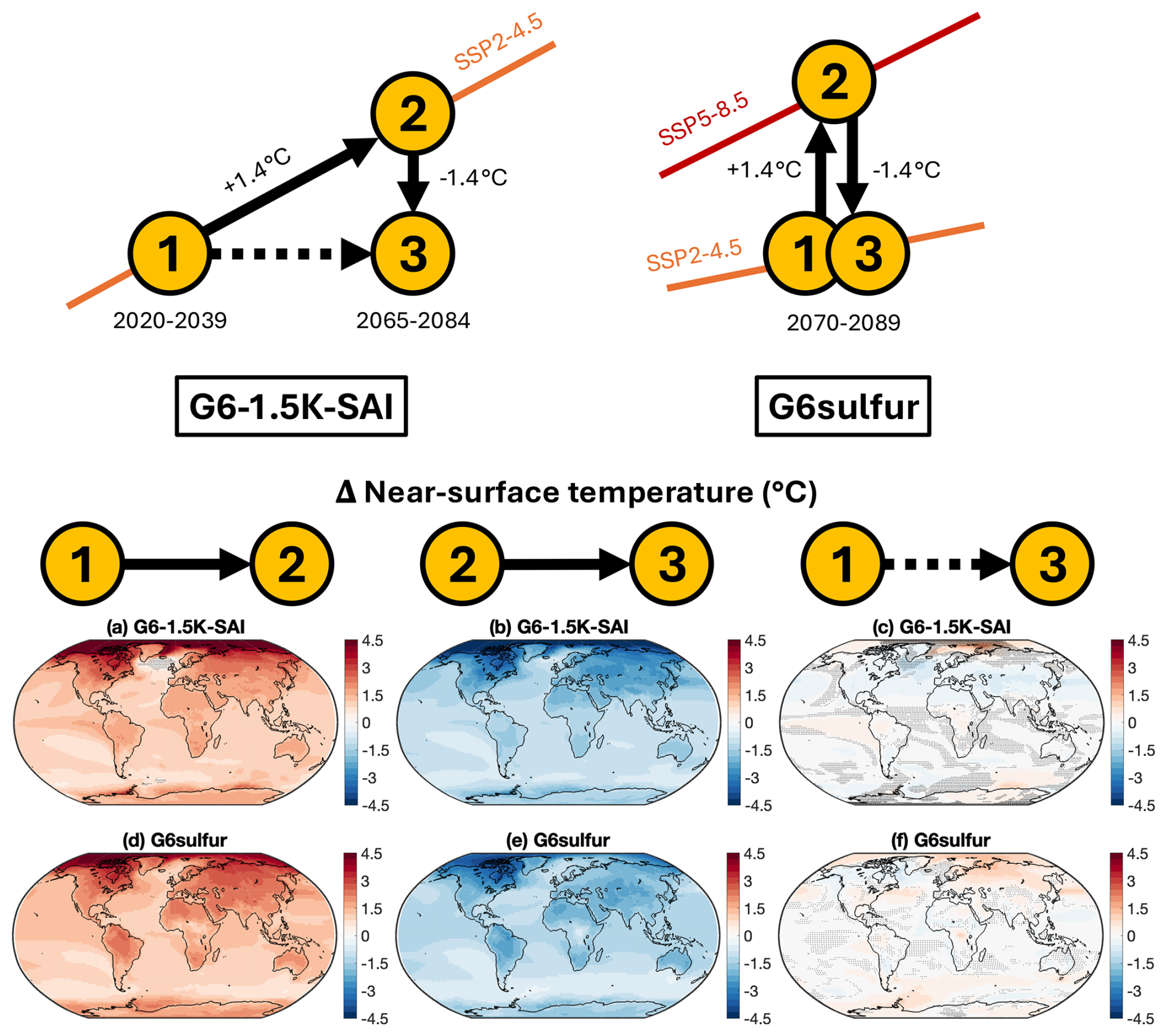
Figure 2 From Lee et al. (2026b): Maps of near-surface air temperature changes (in °C) for G6-1.5K-SAI and G6sulfur multi-model means, between three different periods: (1) the reference period, corresponding to the period over which the GMSAT targets are defined; (2) the warmed world; and (3) the new climate state reached under GHG plus SAI. The left column plots the difference between (1) and (2), representing the impacts of global warming alone; the middle column plots the difference between (2) and (3), representing the impacts of SAI alone; and the right side column plots the difference between (1) and (3), representing the combined impacts of warming and SAI. For G6-1.5K-SAI, period (1) is SSP2-4.5 2020-2039, period (2) is SSP2-4.5 2065-2084, and period (3) is G6-1.5K-SAI 2065-2084. For G6sulfur, all three periods are averages of 2070–2089 data, in which the amount of cooling is approximately the same (1.4 °C) as the last 20 years of G6-1.5K-SAI. Shading represents areas where models disagree on the sign of the change (fewer than 3 out of 4 for G6-1.5K-SAI, and fewer than 4 out of 6 for G6sulfur).

3.1.2 Simulations set-up

The preparatory experiments described in Table 1 are intended to assist in setting up G7-1.5K-SAI by determining the model's sensitivity to SAI at 30° latitude. With the sensitivity known, injection rates can be chosen to drive the climate towards, and maintain, the PI +1.5 °C temperature target ±0.1 °C. This could be done manually using a “guess-and-check” process, as was done in most models for G6sulfur (Kravitz et al., 2015); however, the process of choosing injection rates is greatly facilitated by the use of a feedback control algorithm, an approach used by some G6sulfur models and all G6-1.5K-SAI models. The preparatory experiments provide sufficient system identification information to write a simple feedback algorithm which can choose the required injection rates in the presence of uncertainty in the response and variability. This process was first used to design a 3-DOF experiment by MacMartin et al. (2017) and Kravitz et al. (2017); while the design process for the original feedback algorithm was quite complex, it is possible to modify their original algorithm for similar 3-DOF and 1-DOF experiments with the following steps. The necessary unknowns are constants, called controller gains, which determine how much SO₂ to inject based on the running deviation from the temperature target. A process for deriving these gains from the original algorithm is described by Lee et al. (2025a) in their Sect. 2.2, but to briefly summarize: if the sensitivity of a climate model (in units of °C per Tg SO₂ yr⁻¹) to 30° N + 30° S injection is known, adequate controller gains for controlling GMSAT with SAI at 30° N + 30° S can be computed, producing a gain in units of [Tg SO₂ yr⁻¹][ °C⁻¹]. The detailed procedure is described in Visioni et al. (2023b) and MacMartin et al. (2017). This gain can then be used to construct a feedback algorithm in the form of Eq. (1) in Lee et al. (2025a).

Models that do not have interactive stratospheric aerosols can still run G7-1.5K-SAI: they can either use their own stratospheric aerosol distribution (as done by both MPI versions in the G6sulfur experiments, and by CNRM (Visioni et al., 2021b)), as long as it looks reasonably symmetrical between the hemispheres, or they can use a scaled version of the CESM2-WACCM6 generated distribution (or other models) for the G6-1.5K-SAI, as proposed in the Climate Chemistry Model Intercomparison CCMI-2022 senD2-sai experiment (Tilmes et al., 2025), to fully simulate the aerosol impacts in the stratosphere. In the latter case, modeling centers can request a data set of aerosol radiative properties (extinction coefficient, single-scattering albedo, asymmetry factor) on their model-specific wavelengths to the GeoMIP co-chairs. Such data will be provided on request – as modeling centers will also have to share the details of their short-wave and long-wave radiative transfer model spectral grids – and prepared with the REtrieval Method for optical and physical Aerosol Properties in the stratosphere (REMAPv1) that was described in Jörimann et al. (2025). In short, the REMAPv1 method works by first retrieving the parameters of a single-mode log-normal aerosol size distribution that represents the input dataset in a best-fit sense. From there, it computes optical properties on any specified wavelengths (or wavelength bands) using Mie theory. In this manner, using REMAPv1, modeling centers can also obtain all necessary aerosol properties from the preparatory Inj-sulf cases described in Sect. 2 from other models to understand their own model's climate response to different patterns of aerosols.

3.2 G7-1.5K-SAI-End

Many members of the community have highlighted the importance of conducting a coordinated experiment that includes an abrupt termination of SAI (Parker and Irvine, 2018) in the context of GeoMIP. Robock et al. (2008) first included an abrupt termination in their SAI experiment using constant yearly emissions of SO₂. A similar experiment was then part of the original G4 experiment (Kravitz et al., 2011), and the climatic responses were then explored in multiple papers (Trisos et al., 2018; Jones et al., 2013); it has now been deemed to be an important inclusion in the CMIP7 simulations in order to offer a more comprehensive picture of potential SAI risks. For this reason, we propose a G7-1.5K-SAI-End experiment that branches off from the G7-1.5K-SAI, abruptly ending SO₂ injections at the end of 2084, and that continues simulations for at least 15 years to understand Earth system responses under an abrupt warming. Simulations with an abrupt termination can also be leveraged to emulate the response under more moderate phase-outs scenarios by expanding the scenario space (Farley et al., 2024), and are also likely to inform assessment of SAI impacts on tipping dynamics and risks therein (Zhao et al., 2025; Lenton et al., 2025; Bednarz et al., 2025a).

3.3 G7-1.5K-HiLLA

As with G7-1.5K-SAI and G6-1.5K-SAI, the G7-1.5K-HiLLA (“High-Latitude, Low-Altitude”) experiment is identical to the earlier G6-1.5K-HiLLA experiment (Duffey et al., 2026), except that it uses the CMIP7 emissions scenario. G7-1.5K-HiLLA matches the global mean temperature target of G7-1.5K-SAI, but instead of year-round subtropical (30°) injection, the G7-1.5K-HiLLA experiment uses spring/early-summer (MAMJ for the NH, SOND for the SH) low-altitude (15 km) injection in the sub-polar latitudes (60°). This is a scenario which aims to represent a plausible early-stage, logistically constrained deployment of SAI (Wheeler et al., 2025), that might be deployable using modified existing aircraft, rather than using novel high-flying ones (Duffey et al., 2025). Unlike for G7-1.5K-SAI, the longitude of injection is prescribed, at 180° E. With lower altitude injection, longitude likely has larger effects than at high altitudes (Sun et al., 2023), and previous HiLLA simulations show non-negligible impacts of varying longitude, particularly in the Southern Hemisphere (Duffey et al., 2026).

Hemispherically symmetric injections are used in the G7-1.5K-HiLLA scenario for the same reasons as the G7-1.5K-SAI case above. As above, this strategy will not perfectly maintain interhemispheric temperature gradient in any model, and there is substantial divergence across models in the zonal mean temperature response under G6-1.5K-HiLLA (Fig. 3), in part due to differences in the model's Arctic amplification in the background SSP2-4.5 warming. In UKESM1-1 and MIROC-ES2H, the substantial high latitude NH residual warming present under G6-1.5K-SAI is reduced under G6-1.5K-HiLLA. Alternatively, overcooling in the NH high latitudes in CESM2-WACCM under G6-1.5K-SAI is increased even further under G6-1.5K-HiLLA.

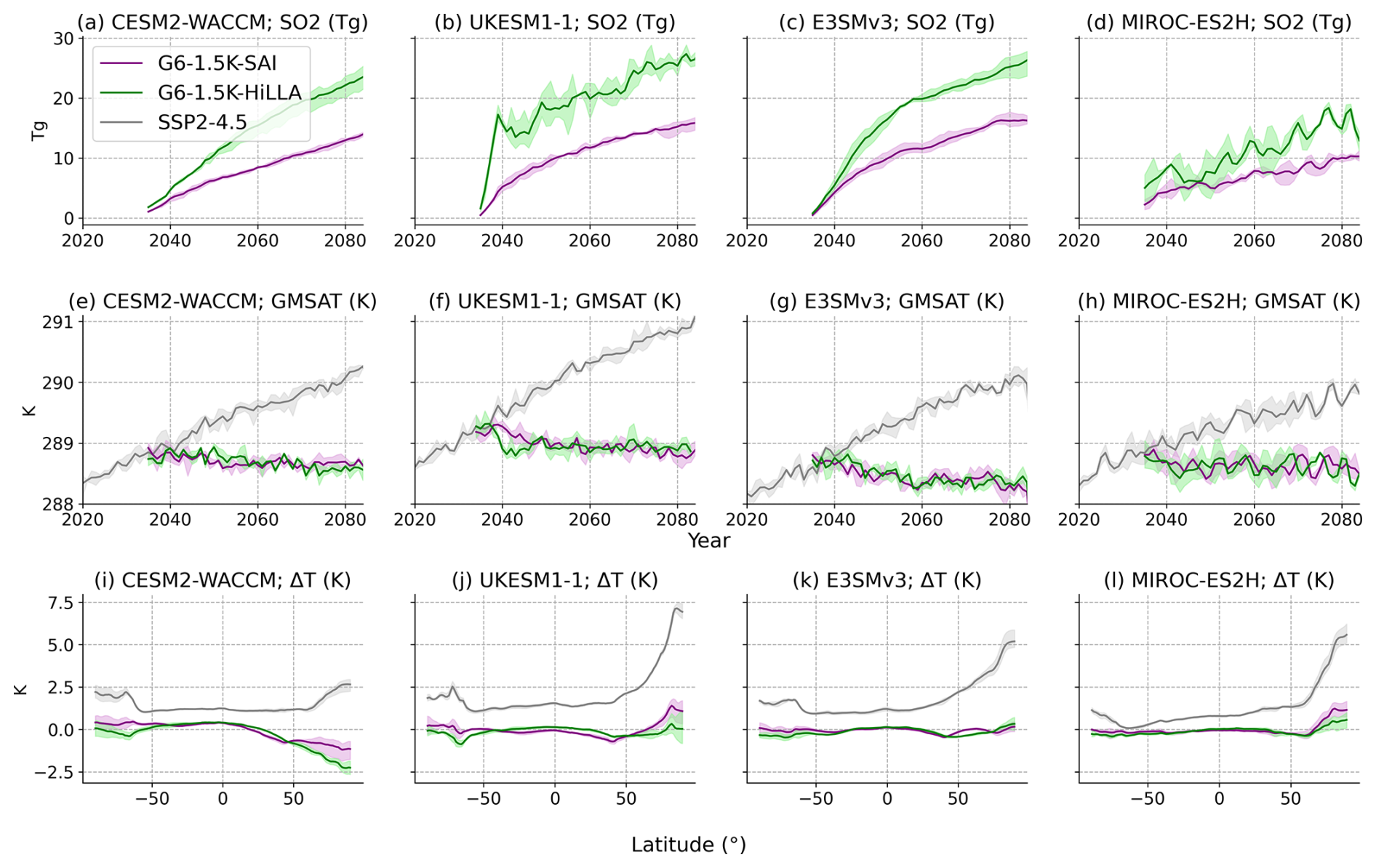
Figure 3 (a–d) Injection magnitude (Tg SO₂), (e–h) Global mean surface air temperature (GMSAT), and (i–l) zonal mean temperature change relative to the 2020–2039 baseline (ΔT), for the four models with G6-1.5K-SAI and G6-1.5K-HiLLA simulations. The solid lines show ensemble means and shaded areas show ensemble range, using the first three members for all scenarios.

3.3.1 Why 15 km injection altitudes?

Testbed simulations (Duffey et al., 2026) indicated a strong dependence on injection altitude under HiLLA strategies, with global mean cooling increased from 0.6 °C per 12 Tg SO₂ to 1.0 °C per 12 Tg SO₂, when altitude is increased from 13 to 15 km. The maximum altitude of various large jetliners is 13 km (Smith et al., 2024), so the G6-1.5K-HiLLA strategy may not represent a logistically feasible strategy with these aircraft. However, given the significant global cooling required to meet the G7-1.5K strategy, and so produce a climate state comparable with G6-1.5K-SAI, the altitude of 15 km was chosen to achieve sufficient cooling efficiency to prevent the need for extremely large injection magnitudes.

3.3.2 Simulations set-up

The experimental setup for G7-1.5K-HiLLA is identical to that of G7-1.5K-SAI, except that 15 km springtime 60° injection is used instead of 21.5 km year-round 30° injection. Once the model sensitivity to 60° injection is known, the injection rates can be determined through the same process outlined in Sect. 3.1.2. Across the four models with simulations of both G6-1.5K-HiLLA and G6-1.5K-SAI, the relative global mean cooling efficiency, ${\displaystyle \frac{E_{\text{HiLLA}}}{E_{\text{SAI}}}}$ (where E is global mean cooling per unit injection), ranges from 0.57 to 0.64 K Tg-S⁻¹ across the four models (0.57 in CESM2-WACCM, 0.64 in UKESM1-1, 0.64 in E3SMv3, and 0.60 in MIROC-ES2H). Equivalently, G6-1.5K-HiLLA requires 1.56 to 1.76 times the injection magnitude of G6-1.5K-SAI to achieve the same target state. Given that injection occurs in only four months in each hemisphere, the rate of SO₂ injection in G6-1.5K-HiLLA is approximately five times higher than that under G6-1.5K-SAI. HiLLA strategies achieve their global mean cooling via greater polar and less tropical cooling than low latitude injection strategies (Fig. 3), and so the HiLLA efficiency would be reduced if defined in terms of the cooling of low latitude regions (Duffey et al., 2026).

3.4 G7-1.5K-MCB

The G7-1.5K-MCB experiment follows the choices made for the G7-1.5K-SAI experiment, except that it uses MCB, and is functionally identical to G6-1.5K-MCB (Hirasawa et al., 2026a) but using the CMIP7 ML emission scenario as its reference. In G7-1.5K-MCB, MCB is applied by injecting sea salt aerosol at the same vertical level as natural sea salt emissions (typically in the lowest level of the atmospheric grid) in grid cells with ocean fraction greater than 0.5 in five midlatitude ocean areas (see Fig. 4f red boxes): the North Pacific (NP: 30 to 50° N and 190 to 120° W), North Atlantic (NA: 30 to 50° N and 70 to 0° W), South Pacific (SP: 50 to 30° S and 170 to 90° W), South Atlantic (SA: 50 to 30° S and 55° W to 15° E), and South Indian Ocean (SI: 50 to 30° S and 30° E to 100° W). We recommend that the injected sea salt aerosols have approximate effective dry radii of 30 to 50 nm if possible, though this may vary depending on the activation parameterization and natural sea salt aerosol representation, as discussed in Sect. 2.2. The total mass of emissions are set to be equal in both hemispheres and at a constant emission rate throughout a given year. MCB is used to maintain GMSAT within ±0.2 °C of 1.5 °C above the preindustrial average by increasing emissions over time to cool global mean surface temperatures to this level. The experiment branches from the ML emissions scenario at model year 2035, and runs until model year 2150.

Figure 4 shows results from the G6-1.5K-MCB experiment conducted using four CMIP6-era ESMs. The global-mean surface temperature is maintained at the 2020–2039 levels of the SSP2-4.5 simulations (Fig. 4c), by injecting sea-salt aerosols in the five midlatitude regions shown in Fig. 4f. The mass required to maintain temperatures at 2020–2039 levels differs substantially between models (Fig. 4a), but much of that difference is due to discrepancies in the size of the emitted sea-salt aerosol such that the number emission rate differs less between models (Fig. 4b). While the warming pattern from SSP2-4.5 (Fig. 4e) is largely offset by the cooling pattern from MCB (Fig. 4g), some residual differences remain (Fig. 4f) with overcooling over the oceans and residual Arctic warming. Models differ on the interhemispheric temperature asymmetry under both SSP2-4.5 and G6-1.5K-MCB (Fig. 4d).

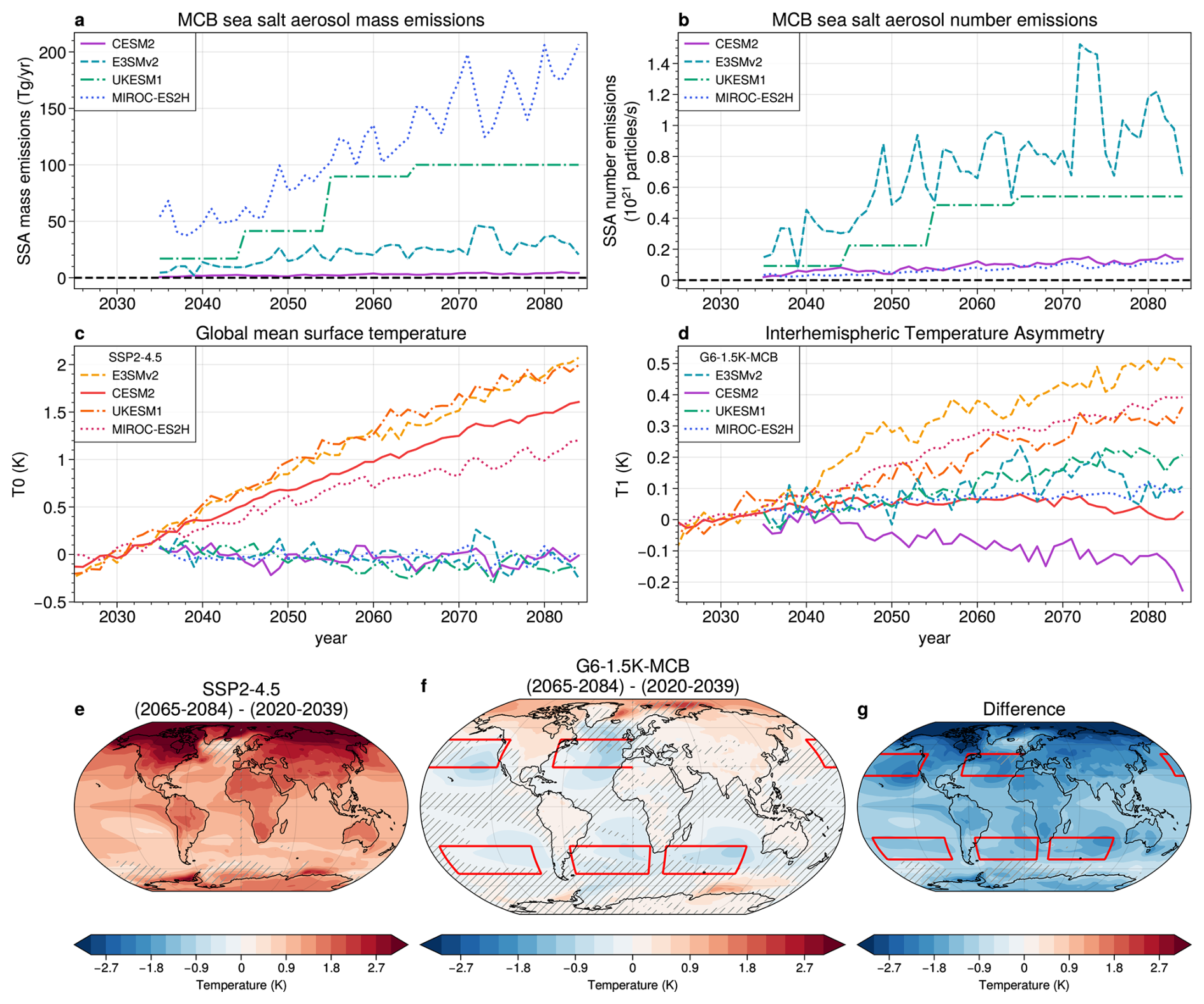
Figure 4 Results of G6-1.5K-MCB simulations in four ESMs (E3SMv2.0, CESM2.1, UKESM1.0, and MIROC-ES2H). Top row shows the sea salt mass flux (a) and number flux (b) required in each model to maintain the 1.5K GMSAT target. Middle row shows the T₀ (c) and T₁ (d) time series for the SSP2-4.5 reference simulations (red shades) and G6-1.5K-MCB simulations (blue shades). Bottom row shows the spatial pattern of annual mean reference height (2 m) temperature anomalies averaged across the models for SSP2-4.5 (e), G6-1.5K-MCB (f), and the difference between the two (g) (the MCB effect). Hatching indicates grid points where at least one model disagrees on the sign of the response.

3.4.1 Why hemispherically mass-balanced injections?

Similar to G7-1.5K-SAI, the MCB equivalent is designed as a one degree-of-freedom strategy that strikes a balance between achieving a climate response that reasonably offsets the greenhouse gas warming effect and remaining simple enough to be implemented by a range of state-of-the-art ESMs (Hirasawa et al., 2026a). Exploratory analysis in three CMIP6 ESMs (Hirasawa et al., 2026b) found that emitting sea salt aerosol into five mid-latitude regions (NP, NA, SP, SA, SI) resulted in temperature and precipitation response patterns that were more spatially uniform, and thus more closely matched the GHG signal, than previously explored MCB strategies that focused on emissions in lower latitude regions (Stjern et al., 2018; Haywood et al., 2023; Rasch et al., 2024; Lee et al., 2025a). Specifically, shifting emission to higher latitudes reduces the tropical overcooling signal associated with 30° S to 30° N emissions used in previous GeoMIP simulations (Kravitz et al., 2013; Stjern et al., 2018) and the La Niña-like cooling signal characteristic of protocols that focused on the tropical Pacific (Jones et al., 2009; Rasch et al., 2009; Haywood et al., 2023; Rasch et al., 2024; Odoulami et al., 2024; Lee et al., 2025a). Following from this, we further define the emission rates in each region such that the areal-sum emissions are $\mathrm{1}/\mathrm{4}$th of the total emissions in each of the two Northern Hemisphere regions (NA and NP) and $\mathrm{1}/\mathrm{6}$th of the total emissions in each of the three Southern Hemisphere regions (SP, SA, and SI) to minimize shifts in ITCZ by distributing the perturbation evenly across the hemispheres.

While hemisphere-symmetric midlatitude MCB emission simulations demonstrate substantial improvements over past protocols, it is unlikely to be an optimal distribution for returning climate to early-21st century conditions (Fig. 2d, f). Considering the distinct response patterns for MCB in different regions (Hirasawa et al., 2026b), further optimization is feasible (Mason et al., 2026). However, the optimal MCB emission distribution will differ across models due to differences in aerosol-cloud interactions (giving rise to different regional forcing strengths) and atmosphere-ocean circulation and climate feedbacks (giving rise to different patterns of climate response under global warming and under MCB). For G6-1.5K-MCB, UKESM1.1 and MIROC-ES2H show Arctic under-cooling, which indicates MCB in an additional region at polar latitudes may be required in these models (Mason et al., 2026; Henry et al., 2025). CESM2 shows NH cooling relative to the SH while E3SMv2 shows NH warming relative to the SH, which suggests additional MCB should be applied in the Southern hemisphere in CESM2 and in the NH in E3SMv2. Furthermore, CESM2 simulations that balanced the sea salt mass emissions to produce equal forcing in each hemisphere produced excessive NH cooling and southward shifts in the ITCZ (Hirasawa et al., 2026a). These variations across models demonstrate that there is not a single emission distribution that would maintain the hemispheric asymmetry consistently across all models and that forcing is not necessarily a good predictor of hemispheric temperature response due to differences in radiative feedbacks and circulation response. Thus, to maintain simplicity in model configuration and to ease the interpretation of inter-model differences, we select mid-latitude MCB with mass emissions distributed evenly between the NH and SH as the basis of a 1-DOF design as a first-order attempt to reduce inter-hemispheric asymmetries.

3.4.2 Simulations set-up

The Inj-seasalt-midlat experiment described in Table 1 and Sect. 2.2 is designed to determine a given model's sensitivity to mid-latitude MCB, which can be used to set up G7-1.5K-MCB. With this sensitivity known, the sea salt aerosol injection rates can be chosen to maintain the GMSAT target. This can be done by adjusting emissions manually over the simulation period (“guess-and-check”) or by using a feedback controller algorithm. Inj-seasalt-midlat provides information on the magnitude and time scale of the cooling response to mid-latitude MCB at a given emission rate, which are the two key pieces of information for computing the parameters of a 1-DOF feedback controller (see Appendix A of Hirasawa et al., 2026a). The time scale of climate response to MCB tends to be longer than the response to SAI, thus the feedback gains required for a G7-1.5K-MCB controller may differ from those used in a G7-1.5K-SAI controller. The MCB forcing is inherently non-linear, due to the sub-linear behaviour of aerosol activation (Rasch et al., 2024). This makes it challenging to estimate a full MCB emission time series prior to running a scenario simulation (also known as a “feedforward” estimate), because the model sensitivity derived from Inj-seasalt-midlat will be an underestimate early on in the simulation, when emissions are still low, and an overestimate late in the simulation, when clouds become saturated with aerosol. We also note that anthropogenic aerosol emissions are projected to decrease in future scenarios which would make clouds more susceptible to brightening by MCB (Sun et al., 2026a), but this has not been quantified in ESMs. Feedback controllers can partially account for such nonlinearities, as they can adjust emissions in response to these deviations.

3.4.3 Alternate Cloud Droplet Number Concentration set-up

While we expect that most CMIP7 generation ESMs will be capable of increasing accumulation mode sea salt aerosol, some may have limitations that prevent adequate representation of G7-1.5K-MCB with sea salt aerosol emissions. For such models, it may be more practical to directly perturb the cloud droplet number concentration (CDNC) in the five midlatitude MCB regions (see Hirasawa et al. (2026a) Sect. 2.4 for simulation descriptions). CDNC perturbations have been used in several past MCB simulation protocols (Rasch et al., 2009; Kravitz et al., 2013; Hirasawa et al., 2023; Chen et al., 2025; Lee et al., 2025a) and we expect that sea salt aerosol injection and CDNC perturbation simulations will produce similar climate responses, if they are calibrated to produce the same radiative forcing (Rasch et al., 2024). Nevertheless, this method is idealized and neglects key processes like aerosol activation, aerosol transport, and aerosol direct forcing, potentially underestimating the inter-model uncertainty. Thus, we recommend using sea salt aerosol emissions when possible.

4 Tier 2 experiments

Over time, different modeling groups have devised their own specific SRM experiments, either selecting different scenarios and targets, or proposing new methods or deployment strategies, based on different interests and needs; it is neither possible nor advisable to claim each one of them should be an official GeoMIP experiment. However, it was suggested during the last few GeoMIP meetings to have a central space to collect ideas and identify other groups interested. Therefore, in this section we collect a series of lower priority experiments that can be run in order to enrich the analyses from the Tier 1 experiments. Considering the potential infinite space of experiments, it will be important for modeling teams and research groups to communicate promptly about what experiments they are running so that an up-to-date registry of ongoing Tier 2 experiments can be kept on the GeoMIP website, similarly to what was proposed in Kravitz et al. (2015) for test-bed experiments. This may be useful, for example, to generate spin off working groups focused on mechanistic investigation to further inform interpretation of Tier 1 simulations. In general Tier 2 simulations can be categorized as scenario exploration, SRM strategy exploration, and process level understanding, and will be discussed in turn below.

4.1 Tier 2 experiments exploring different scenarios

This set of experiments is meant to extend exploration of scenarios through the inclusion of different amounts of cooling (G7-0.5K-SAI), a different underlying scenario (G7-1.5K-SAI-LN), or the exploration of a delayed start (G7-1.5K-SAI-Late). These scenarios are shown in Fig. 5. This set is not meant to be comprehensive, but rather to suggest the capacity to run further experiments with scenarios of interest.

Table 3 Scenario exploration Tier 2 experiments. GMSAT = Global Mean Surface Air Temperature; SAI = Stratospheric Aerosol Injection; ML = Medium-Low scenario (van Vuuren et al., 2025); LN = Low-to-Negative scenario. As we don't expect all modeling teams to perform these experiments, and they are not comprehensive nor prescriptive, no total amount of years of simulation is provided.

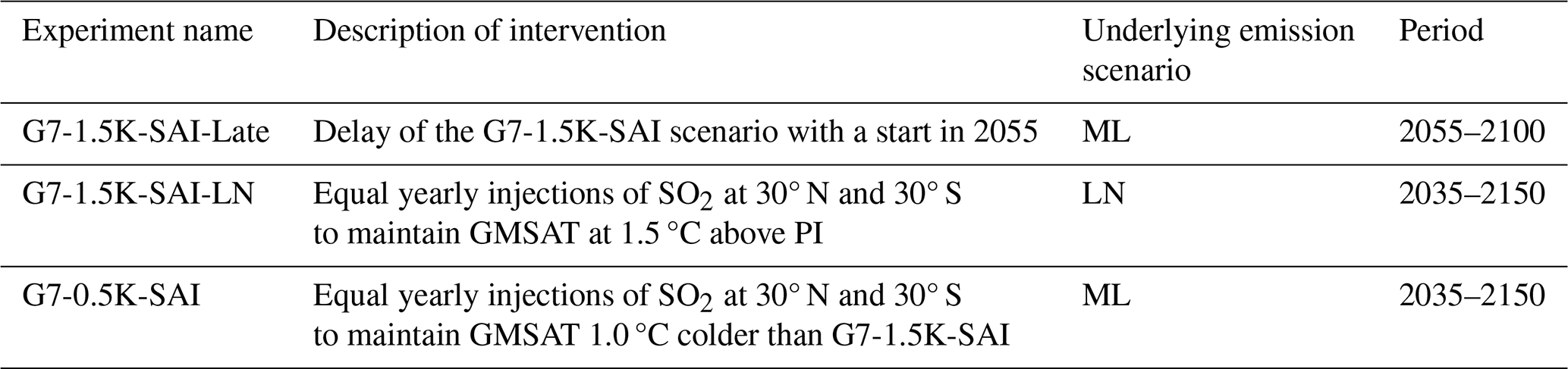
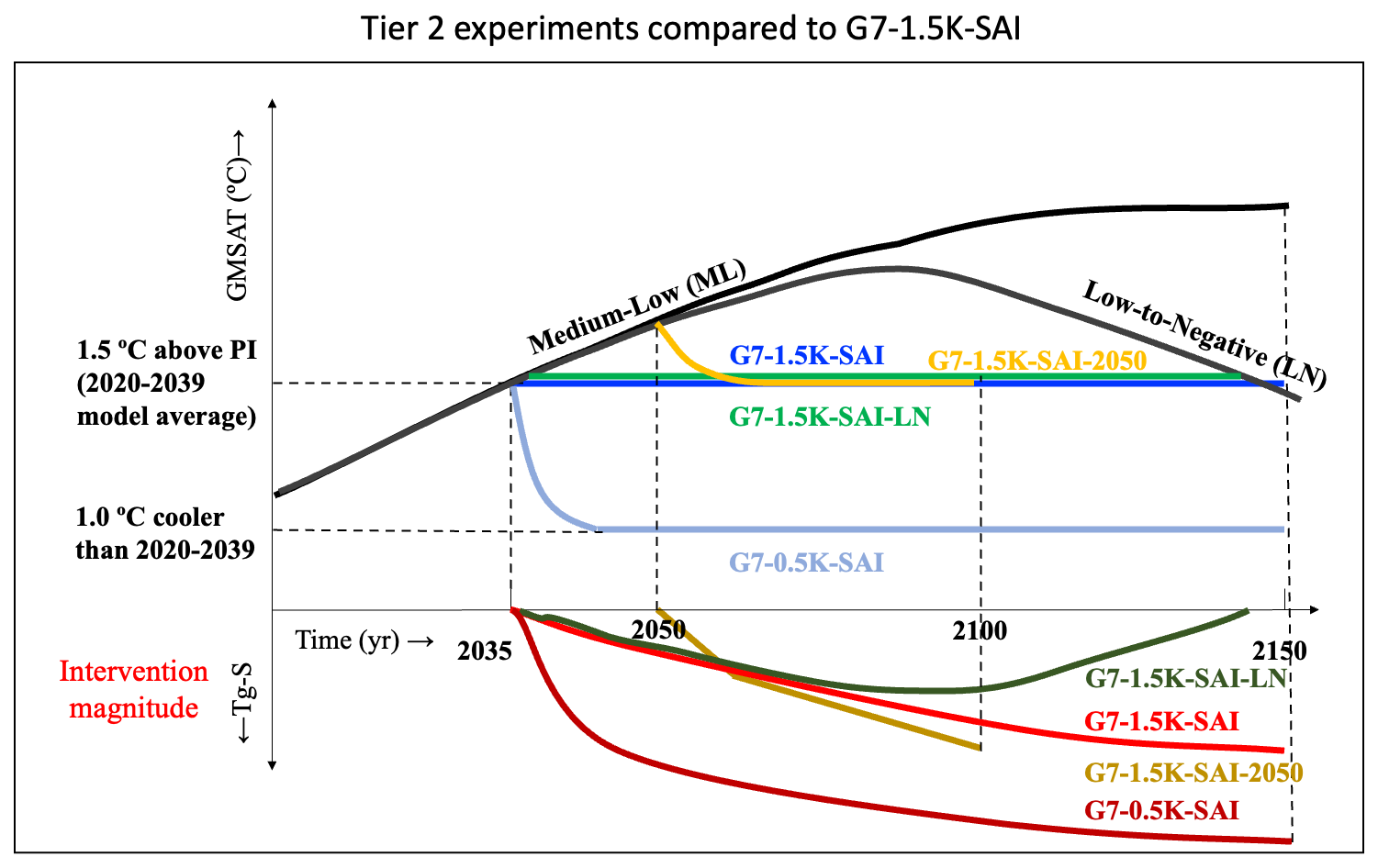
Figure 5 Schematics of Tier 2 scenario exploration experiments for the SAI case, with the inclusion of main Tier 1 scenario (G7-1.5K-SAI) for comparison.

The importance of considering a larger range of scenarios, including both higher or lower cooling targets and the inclusion of changes in the deployment (i.e. interruptions, phase-outs) has been highlighted before (MacMartin et al., 2022). While this space is potentially infinite, and highly dependent on the assumptions of the underlying emission scenario (Baur et al., 2023), there is clearly merit in both considering different degrees of cooling (Visioni et al., 2023b), as well as potential inconsistencies in deployment (Farley et al., 2024), and the results of such broader set of simulations can also be included in emulators that already integrate GeoMIP data (Martínez Montero et al., 2022; Muñoz-Sánchez et al., 2025; Farley et al., 2026). Here we provide some suggestions of how such an expanded exploration could look, leaving some choice to modeling groups with different interests to expand on this, as long as some coherence through the common simulation of Tier 1 experiments is maintained, as was done previously (Tilmes et al., 2020; Baur et al., 2025).

• G7-0.5K-SAI. a potential case cooling 1 K more than the G7-1.5K-SAI case, which would lead to a higher rate of deployment, and which could be compared against the 1.5 K to understand trade-offs between more cooling and other relevant surface climate impacts such as air quality impacts (Wang et al., 2026) and agricultural impacts (Clark et al., 2023), as well as to investigate the efficacy of SRM strategies to reduce climate risk including risks associated with tipping elements against the backdrop of a greater masking of GHG induced warming. The larger injection needed to cool by that amount should be ramped up linearly over the first 10 years as done in the ARISE-SAI-1.0 case (Brody et al., 2024).

• G7-1.5K-SAI-LN. a potential case could explore having the same cooling target as G7-1.5K-SAI, but on a lower (LN) or higher (M) underlying emission scenario, to look at different impacts under different scenarios, as proposed in the test-bed experiments described in Tilmes et al. (2020) using the SSP5-3.4OS temporary overshoot experiment.

• G7-1.5K-SAI-Late. some studies have recently explored the differential impacts of an SAI deployment depending on the starting date, highlighting differences in ocean heat uptake and stratospheric ozone changes due to different chlorine loads in the stratosphere (Brody et al., 2024; Pflüger et al., 2024). This type of experiment is further motivated by calls to understand the ability of SAI to reverse GHG driven changes to drivers of climate tipping in the cryosphere, biosphere, ocean and atmosphere, which include the deceleration of AMOC (Pflüger et al., 2024), melting of glaciers and permafrost, and risk of amazon dieback, among others (Lenton et al., 2025). Delayed implementation studies may support greater understanding of what SAI can and cannot do as a function of the timing of deployment during this century. For a GeoMIP experiment, we propose a delay of 15 years compared to the start of G7-1.5K-SAI, and to run the experiment for at least 50 years.

This potential set of experiments, in a multi-model context, would be extremely useful when thinking about the broader context of emission trajectories, temporary temperature overshoot dynamics and climate stabilization more broadly (Palazzo Corner et al., 2023); the comparison of experiments with different underlying emission scenarios, and/or between different cooling targets, can shed light on how SRM would impact carbon cycle dynamics (Zhao et al., 2024) (considering the emission-driven pathways in CMIP7 models (Meinshausen et al., 2024)), and how it compares to net-zero and negative emission scenarios using Carbon Dioxide Removal (CDR) (Sanderson et al., 2025); as well as feed into discussions of the reversibility or irreversibility of specific climatic changes, and of tipping elements dynamics in the context of SRM (Hirasawa et al., 2023; Zhao et al., 2025; Lenton et al., 2025), especially as it pertains to different degrees of warming, or timing, at which climate stabilization may occur (Winkelmann et al., 2025; Pflüger et al., 2024).

4.2 Tier 2 experiments exploring different SRM strategies

Together with an exploration of different scenarios as discussed in the previous section, there is significant interest in coordinating simulations for other SRM strategies. These include variations on SAI and MCB to explore the influence of intervention location and material, as well as process-oriented inter-comparisons of other SRM proposals. Here, we outline several experiments based on previous and ongoing modeling work. This list is not comprehensive and we encourage groups to explore the scenario and strategy space.

Table 4 Strategies exploration Tier 2 experiments. GMSAT = Global Mean Surface Air Temperature; SAI = Stratospheric Aerosol Injection; DOF = Degrees of Freedom; MCB = Marine Cloud Brightening; ML = Medium-Low scenario (van Vuuren et al., 2025). As we do not expect all modeling teams to perform these experiments, and they are not comprehensive nor prescriptive, no cumulative sum for the years of simulation for all experiments is provided.

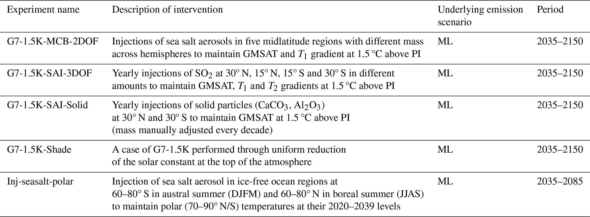
A non-comprehensive set of potential experiments is provided in Table 4, and might include:

• G7-1.5K-MCB-2DOF. Climate model analyses have pointed out the importance of minimizing inter-hemispheric temperature gradients, as single-hemisphere MCB perturbations can cause dramatic shifts in tropical precipitation (Emme et al., 2025). Modeling groups may therefore consider an iteration on the G7-1.5K-MCB in which the areal-sum emission rate in each hemisphere is adjusted to manage two degrees of freedom (2DOF) – the GMSAT and the inter-hemispheric temperature gradient (T₁). This may require additional preparatory experiments in which MCB emissions are applied in each hemisphere independently for the reasons described at the end of Sect. 3.4.1. While a 3DOF case aligning with SAI may enable clearer inter-method comparison, more research would be required to determine how well the equator-to-pole gradient could be controlled through different MCB deployment patterns.

• G7-1.5K-SAI-3DOF. Modeling groups interested in developing more comprehensive, targeted simulations of SAI by better understanding the design space of SAI in their model, should consider running a case of G7-1.5K-SAI trying to manage 3 degrees of freedom (DOFs), using the same protocol as ARISE-SAI (Richter et al., 2022). This is a more complex injection protocol than G7-1.5K-SAI, but is designed to yield smaller regional temperature differentials relative to the target period. In this protocol, GMSAT, interhemispheric temperature gradient, and equator-to-pole temperature gradient (referred to as T₀, T₁, and T₂, respectively, by Richter et al., 2022) are simultaneously maintained at PI+1.5 °C (2020-2039) levels. This is accomplished with injections in independent amounts at 30° N, 15° N, 15° S, and 30° S, with injection rates chosen based on the various Inj-sulf preparatory experiments described in Sect. 2.

• G7-1.5K-SAI-Solid. Stratospheric heating through the absorption of (mainly) terrestrial radiation by sulfate aerosols not only affects stratospheric climate, but also surface climate, as demonstrated in Wunderlin et al. (2024); Simpson et al. (2019); Visioni et al. (2021a). To minimize stratospheric heating, several studies have proposed alternative, solid materials for stratospheric aerosol injections (e.g., Dykema et al., 2016; Vattioni et al., 2024a, and references therein). In a single-model study Stefanetti et al. (2024) have found calcite, alumina, and diamond nano-particles to alleviate absorptive heating, while the latter also results in a greater surface cooling efficiency, i.e. requiring smaller injection masses for a given temperature target. Ozone changes could also be reduced through the use of solid particles, although substantial uncertainties remain around the actual chemistry impacts of materials not usually found in the stratosphere (Vattioni et al., 2023, 2025). To improve the robustness of solid aerosol injection modeling, some modelers perform activities within SolidMIP, an active community under the GeoMIP umbrella, focused on the intercomparison of model development work around solid particle SAI and uncertainties in physico-chemical and optical properties of various alternative materials. Within SolidMIP some modeling centers are working towards a case of G7-1.5K-SAI using solid particles instead of sulfate precursors, to lay the groundwork for a future coordinated multi-model approach involving more groups. G7-1.5K-SAI-Solid will consist of two simulations in addition to G7-1.5K-SAI, one for each proposed solid material: calcite (CaCO₃) and alumina (Al₂O₃). Even though Stefanetti et al. (2024) also considered diamond (C(diam)) nanoparticles, which showed the best cooling efficiency and least side-effects, we omit it here because of the recent findings showing that actual industrial diamonds have hybridized impurities substantially deteriorating its optical properties (Kumar et al., 2026). Simulations with the remaining two solid aerosol particle types will be performed in one or more models with full microphysical and radiative treatment of the stratospheric solid aerosol. The injection amount in these preparatory simulations will be manually adjusted to maintain the 1.5 K temperature target, with models' response provided in similar experiments as those proposed in Sect. 2 for the Inj-Sulf-30N/S cases but using fixed amounts of solid particles. The resulting forcing from G7-1.5K-SAI-Solid will then be provided to the community and can be tailored to each individual model as required using the forward Mie calculation part of REMAPv1 (Jörimann et al., 2025). The introduction of the same forcing into different models will provide a range of temperature responses both at the surface and in the atmosphere that can be analysed as a first step. While extremely important to capture the whole balance of potential impacts from solid particles injections, detailed chemical effects will not be included in this first set of simulations for simplicity, and due to the larger uncertainties for those materials (Vattioni et al., 2025).

• Inj-seasalt-polar. Henry et al. (2025) performed Arctic MCB cooling simulations with sea salt emissions between 60 and 80° N where there is no land or sea ice in a sub-set of models used for G6-1.5K-MCB (Hirasawa et al., 2026a). Arctic MCB successfully maintained Arctic mean temperatures and the models suggested there were few significant lower-latitude precipitation impacts, in contrast to single-hemisphere high latitude SAI (Lee et al., 2023). In one model (UKESM1), it was found that there is an upper limit on the possible cooling in the Arctic by MCB (Henry et al., 2025), suggesting a larger inter-model comparison of sensitivity experiments is warranted. We suggest an idealized polar MCB case with sea salt aerosol emissions in ice-free ocean regions between 60 and 80° in both hemispheres during the summer months when insolation is the highest (JJAS in the NH and DJFM in the SH) with step emissions following the preparatory experiment protocols in Table 1.

• G7-1.5K-Shade. Modeling groups interested in diagnosing and separating the aerosols-driven changes on surface climate should consider running an experiment similar to G6solar, in which the same temperature target is achieved through a uniform reduction of incoming solar radiation at the top of the model. This has proven beneficial in highlighting aerosols-driven uncertainties (Visioni et al., 2021b). Furthermore, these simulations would prove beneficial in understanding the impacts of potential space sunshades (Fuglesang and de Herreros Miciano, 2021).

• Combination and contrast of SRM methods and other techniques. There is increasing discussion and opportunity to think of experiments that include a potential “cocktail” of different SRM techniques (Cao et al., 2017), such as for MCB combined with SAI. Future work could explore and define a protocol for such experiments, which we do not yet propose here currently. Similarly, there should be the opportunity to explore the combination of some SRM techniques with other climate intervention proposals that fall more within the realm of changes in atmospheric composition, such as CO₂ removal (Clark et al., 2025) or methane removal (Li et al., 2023), or localized albedo modification techniques (Moore et al., 2021), in order to understand potential synergies as well as unforeseen negative interactions between them. Simulations that achieve the same temperature target as G7-1.5K with carbon or methane removal alone can also be useful to understand differences in the surface climate responses across intervention types (Laakso et al., 2020).

4.3 Mixed-Phase Cloud Thinning experiments

Besides the combination of SAI and MCB discussed in the previous section, another promising approach to polar climate intervention is Mixed-Phase Cloud Thinning (MCT). MCT is a proposed radiation modification method that exploits the thermodynamic instability of mixed-phase clouds – clouds containing supercooled liquid droplets coexisting with ice crystals at temperatures between approximately 0 and $-\mathrm{39}{}^{\circ }$C. By seeding these clouds with ice-nucleating particles (INPs), liquid droplets are converted to ice via heterogeneous freezing, triggering the Wegener-Bergeron-Findeisen (WBF) process that further depletes liquid water (Toll et al., 2024; Villanueva et al., 2025). The resulting glaciated cloud has a lower optical depth and shorter lifetime, reducing its longwave cloud radiative effect; over the polar oceans in winter, where mixed-phase clouds exert a net longwave warming that dominates over shortwave cooling, MCT thus produces a net surface cooling (Villanueva et al., 2022). Despite growing interest in MCT as a polar climate intervention, no coordinated multi-model protocol had previously been proposed; here we report initial findings from a first multi-model intercomparison effort – MCT-MIP Level 0 – and outline a CMIP7-aligned Level 1 protocol (MCT-L1). Information about the required data output for these simulations is provided in Sect. 5.1.

Table 5 MCT-L1 Tier 2 experiments. MCT = Mixed-phase Cloud Thinning; INP = Ice-Nucleating Particles; SST = Sea-Surface Temperature. Both configurations are atmosphere-only and perturb the INP concentration used for heterogeneous freezing (see Sect. 4.3 for the full protocol and Table 7 for the detailed simulation matrix).

4.3.1 Level 0: Initial multi-model results

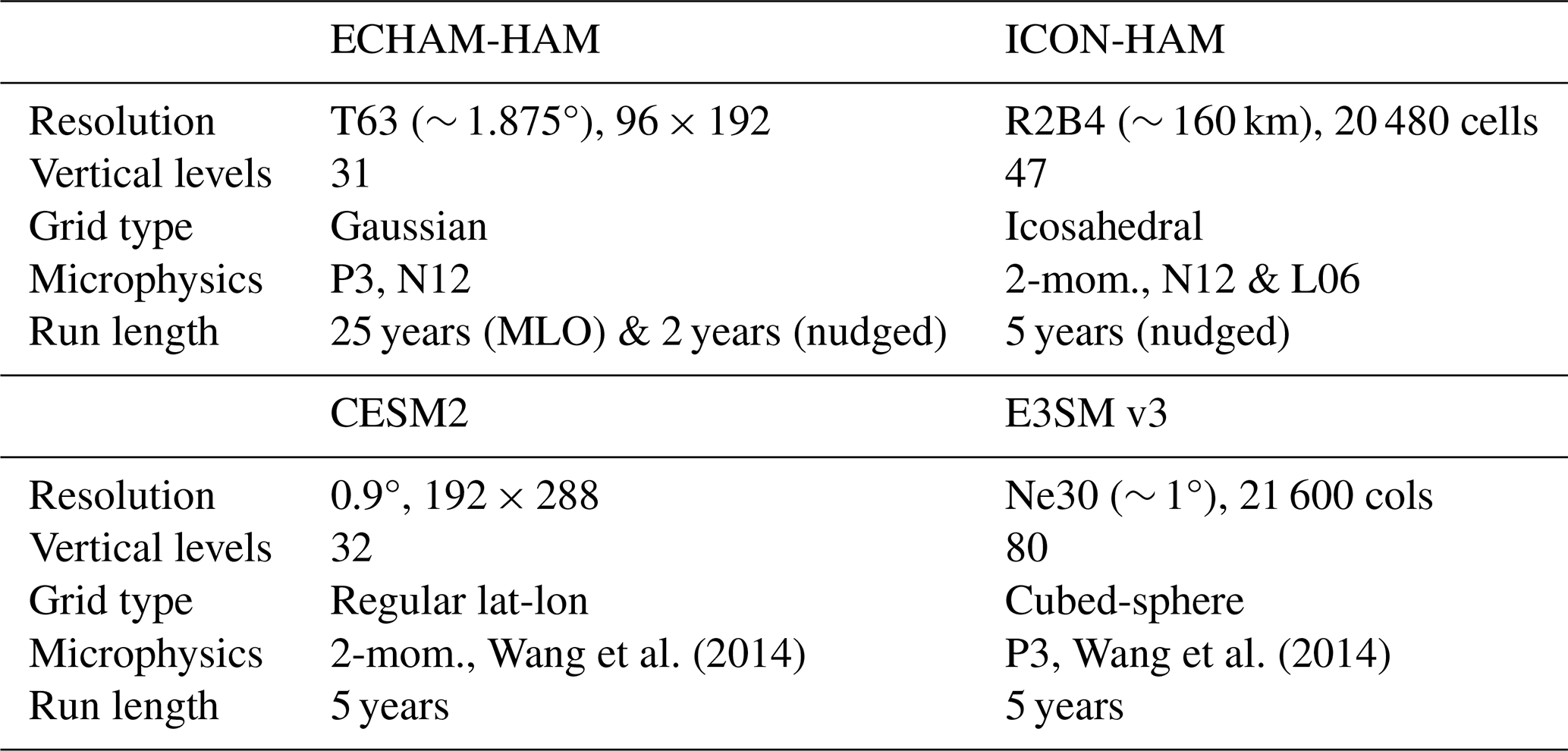
The Level 0 protocol was designed to be broadly implementable: atmosphere-only simulations with prescribed, fixed sea-surface temperatures and sea-ice fractions. Perturbations were done over the polar ocean domain (including sea-ice) poleward of 60° N and 60° S. This corresponds to spatially uniform, winter-only (November, December, January, and February) additions to the dust cloud-borne concentration that is used as input for calculating droplet freezing, alongside an unperturbed control. The perturbation strength was 10⁴, 10⁵, and 10⁶ L⁻¹. Because only the inputs to the droplet-freezing calculations were perturbed, this can be interpreted as a “transparent” aerosol perturbation, decoupled from any side effects associated with direct radiative effects. Simulations used present-day (year 2000; repeating if possible) boundary conditions and ran for a minimum of 5 years (2 years for nudged models), with a 1-year spin-up discarded for free-running integrations. Four models participated (Table 6): ECHAM-HAM, ICON-HAM, CESM2, and E3SMv3.

Wang et al. (2014)Wang et al. (2014)

Table 6 Models participating in MCT-MIP Level 0, with their atmospheric grid and run configuration. MLO: Mixed-Layer Ocean. N12: Niemand et al. (2012); L06: Lohmann and Diehl (2006).

The spatial distribution of the cloud radiative effect (CRE) response during the November–February season (NDJF) is shown in Fig. 6 for all four models at the mid INP level (10² cm⁻³). Three of the four models produce a net cooling with increasing INP concentration, consistent with the expected MCT mechanism; E3SMv3 is an outlier, showing a warming response.

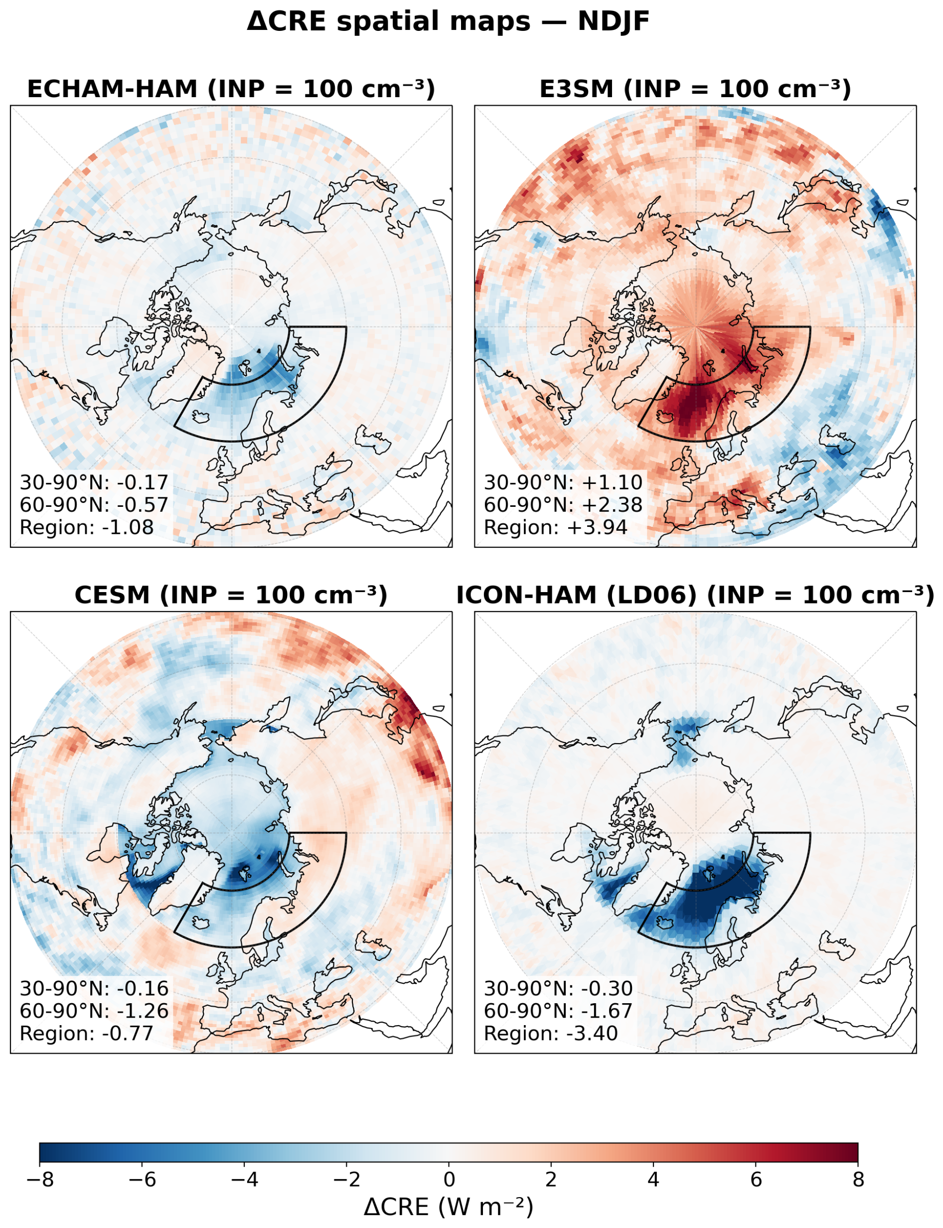
Figure 6 Spatial maps of the net cloud radiative effect perturbation (ΔCRE, W m⁻²) during NDJF for the mid INP level (10² cm⁻³) relative to the control simulation, for all four MCT-MIP Level 0 models. Numbers inset in each panel give the area-weighted mean ΔCRE over 30–90° N, 60–90° N, and the outlined target region (60–90° N, 30° W–90° E, i.e. the North Atlantic–European sector). Blue shading indicates cooling; red shading indicates warming. ECHAM-HAM, CESM2, and ICON-HAM all produce a net negative ΔCRE poleward of 60° N, consistent with the MCT mechanism, while E3SMv3 shows a widespread warming response driven by a base state dominated by very low liquid water content.

The Arctic-mean (60–90° N) NDJF responses of CRE, ice water path (IWP), liquid water path (LWP), and total water path (TWP; from the Cloud_cci v3 product, Stengel et al., 2020) as a function of INP concentration are shown in Fig. A2. CESM2 and ICON-HAM show a clear reduction in LWP with increasing INP concentration, consistent with the MCT mechanism, while E3SMv3 maintains very low LWP across all perturbation levels. Note that the ECHAM-HAM (MLO) configuration is shown for reference only; this idealized perturbation (Villanueva et al., 2022) was designed to maximize the droplet freezing rate (1 % of droplets freeze per hour) and is not directly comparable to the dust-based INP seeding protocol used by the other simulations.

Investigation of the E3SMv3 case reveals a base state in which cloud ice strongly dominates over liquid (Fig. A2b–c), suggesting that clouds in the perturbed domain are already in a saturated-ice regime where the WBF process cannot operate effectively and additional INPs likely suppress the WBF process even further, by decreasing the size of ice particles and slowing down riming and sedimentation. This result underlines the importance of constraining the mixed-phase cloud liquid/ice partition against observations in future intercomparisons.

The sensitivity of the cooling to INP concentration also varies substantially across the three responding models, and the lowest perturbation level (10⁴ L⁻¹) already produces a strong response in total water path (Fig. A2c), motivating the extension to lower concentrations in the next Level 1 intercomparison.

4.3.2 Level 1 protocol: First MCT contribution to GeoMIP

As in Level 0, MCT-L1 simulations are atmosphere-only with prescribed present-day SSTs and sea-ice fractions, with the INP perturbation implemented as a transparent addition to background dust (modifying only freezing rates, without a new tracer). The perturbation range is revised to 10², 10⁴, and 10⁶ L⁻¹ to better characterize the onset of the MCT response at low concentrations. In addition, participating models are encouraged to run a complementary batch in which the background INP concentration from the control is multiplied by 10⁻², 10⁻⁴, and 10⁻⁶, probing the sensitivity to a lower INP mean-state concentration. It is expected that such experiments can help clarify how the INP mean-state of models affects their MCT response.

Table 7 MCT-L1 simulation matrix (7 simulations total). MCT-L1-Seeding perturbations add a spatially uniform INP concentration to the background dust; MCT-L1-Background perturbations scale the control background by the given factor.

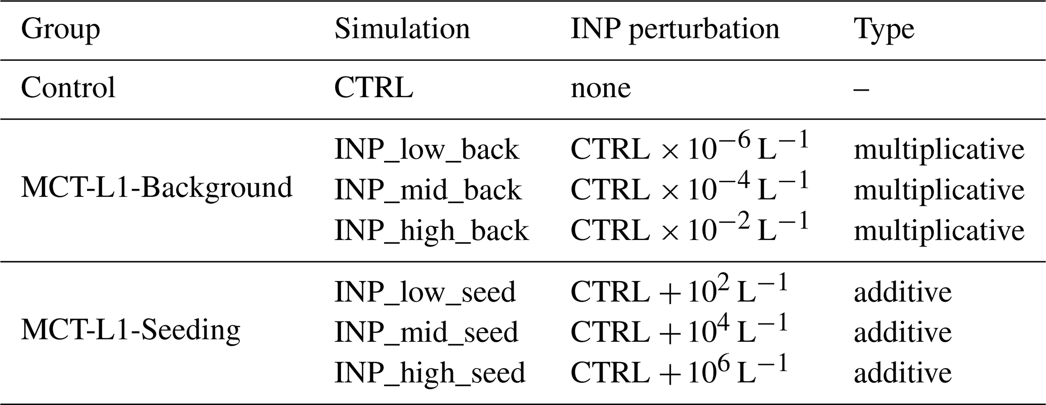
The full set of 7 simulations (1 CTRL + 3 MCT-L1-Seeding + 3 MCT-L1-Background) is designed to map the complete range of mixed-phase cloud responses to INP forcing and to reveal base-state biases of the kind identified in Level 0.

4.3.3 Nudging

Wind-only nudging to ERA5 reanalysis is strongly encouraged to suppress internal variability and enable meaningful multi-model comparison; free-running simulations with a minimum of 10 years are an acceptable alternative.

4.4 Process understanding Tier 2 experiments

This set of experiments is more targeted towards “idealized” scenarios and, like the preparatory experiments, is more targeted towards better understanding of the outcomes of the Tier 1 and some Tier 2 experiments.

Table 8 Process understanding Tier 2 experiments. GMSAT = Global Mean Surface Air Temperature; SAI = Stratospheric Aerosol Injection; DOF = Degrees of Freedom. As we do not expect all modeling teams to perform these experiments, and they are not comprehensive nor prescriptive, no total for the years of simulation is provided.

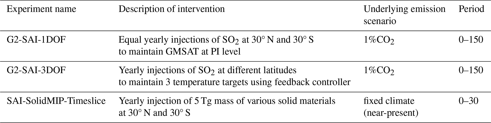
• G2 simulations. The G2 experiment was proposed by the original paper introducing GeoMIP (Kravitz et al., 2011). In the G2 experiment, solar dimming was used to offset forcing from annual 1 % increases in CO₂ concentrations (“1%CO₂ forcing”) against a pre-industrial control (PIcontrol) background. Future warming scenarios include not only GHG forcing, but also evolving aerosol emissions and land use; modeling SRM against a PI control background allows for an evaluation of the impacts of SRM in the absence of these changes. Additionally, beginning SRM at the same time as GHG forcing begins means there is no long-term drift in the background climate state at the start of the experiment.

  Lee et al. (2026a) revisited the G2 experiment by modeling contemporary SAI strategies against PI control + 1%CO₂ forcing for 150 years, with injection beginning the same year as 1%CO₂ forcing begins. They simulated two different strategies: the 1-DOF strategy used in G6-SAI (hemispherically symmetrical injection at 30° to manage global mean temperature) and the 3-DOF strategy used in ARISE-SAI-1.5 (independent injections at 30° N, 15° N, 15° S, and 30° S to manage global mean temperature and the interhemispheric and equator-to-pole temperature gradients simultaneously). Modeling groups interested in understanding the long-term impacts of SAI, and in the importance of background scenario on SAI impacts, should consider running similar experiments.

• SAI-SolidMIP-Timeslice simulations. In addition to the G7-1.5K-SAI-Solid experiment, there is another, time-slice, experiment with solid particles for SAI that is being developed by some in the community, currently consisting of two models (SOCOL-AERv2, Vattioni et al., 2024b and WACCM6-CARMA, Tilmes et al., 2026) with sectional aerosol treatment. While some activities are coordinated with GeoMIP Tier 1 experiments earlier described in this paper, the SAI-SolidMIP-Timeslice experiment follows its own protocol to focus on process understanding in an idealized setting. The experiment design is similar to the ${\mathrm{SO}}_{\mathrm{2}}/{\mathrm{H}}_{\mathrm{2}}{\mathrm{SO}}_{\mathrm{4}}$ protocols described in Weisenstein et al. (2022), based on the atmospheric state fixed to 2040 (this includes all standard forcing such as, GHG, ozone depleting substances levels, tropospheric aerosols, etc.) and the ocean is prescribed with decadal (2020–2029) climatologies of SST and sea ice cover. This climatically stable setting is then used to test various materials under symmetrical 30° N and 30° S single-point constant injections of 5 Tg of material per year. Such a configuration allows intercomparing microphysical and transport processes of solid particles and testing their further upgrades such as new measurements of refractive indices and surface chemistry. Optical properties resulting from these experiments will be then provided to the rest of the SAI community to have a closer look at the uncertainties of the responses in stratospheric dynamics, stratospheric water vapor and stratosphere-troposphere coupling. Chemical effects will be omitted in this first step of involving a wider community, due to the large uncertainties and ongoing laboratory activities associated with chemical reactions on alternative materials.

5 Data request and opportunities

Modeling centers performing GeoMIP simulations should pay close attention to the various data request efforts spearheaded under CMIP7 (Juckes et al., 2025). In particular, the data request efforts for the Atmosphere (Dingley et al., 2026), Earth System (McPartland et al., 2026) and Ocean and Sea Ice (Fox-Kemper et al., 2026) could be particularly important. Furthermore, opportunities to include variables needed by the Inter-Sectoral Impact Model Intercomparison Project (ISIMIP3a) (Frieler et al., 2024) should also be considered.

Simulation of MCB depends on a series of aerosol and cloud processes that must be parameterized in ESMs. Understanding how different processes contribute to inter-model variation in MCB forcing is crucial for constraining the potential cooling from MCB and developing models that can more credibly represent MCB interventions. Variables from the “Diagnosing Radiative Forcing” and “Understanding the role of atmospheric composition for air quality and climate change” opportunities from Dingley et al. (2026) highlight key variables relevant for diagnosing MCB aerosol and cloud responses, which also present notable overlap with required output for DAMIP (Gillett et al., 2025) and AerChemMIP2 (Fiedler et al., 2026). Additionally, cloud condensation nuclei concentrations and subgrid vertical velocity used in prognostic aerosol activation schemes can enable clearer comparisons of cloud droplet activation rates across models, especially for Inj-seasalt-midlat-SST.

High-frequency surface output could be considered in order to investigate the potential for SRM to interact with energy systems (Kumler et al., 2025), as done in Baur et al. (2024b, a): this would require 3 or 6 hourly surface winds and incoming solar radiation, as well as temperature and other meteorological variables such as sea level pressure and humidity that could also be used to diagnose cyclonic activity under SRM (Gabriel Martins Ribeiro et al., 2025). Acknowledging the high burden of providing such data (on both the storage and the analyses side), modeling centers could provide it only for specific time slices (such as the first 10 and last 10 years of simulations for a specific case). In terms of radiation fluxes, we strongly recommend the inclusion of downwelling diffuse shortwave radiation (rsdsdiff). Although sometimes omitted in standard data requests, this variable is essential to accurately assess both crop photosynthesis efficiency and solar power generation under aerosol-altered atmospheric conditions. Providing these variables will greatly enhance the ability of the cross-sectoral impacts community to evaluate the consequences arising from the GeoMIP7 experiments.

Another area with growing interests within the SRM research community that could also leverage high-frequency output is related to analysing extreme events (Tye et al., 2022); this can be better done by using ESM data as boundary conditions for downscaling efforts using Regional Climate Models (RCM) to get better regional information (Wang et al., 2022; Sun et al., 2026b), or using ESM output as a driver for impacts models (Wang et al., 2022). In the case of dynamical downscaling, the models require vertically resolved, sub-daily information, which can be burdensome to save, standardize, and transfer. Nevertheless, the community is clearly at a point where it is ready to engage with these issues, necessitating an explicit request for daily and sub-daily data. To hopefully ease the burden on modeling and analysis groups, we have created a prioritized list of variables that we would like models to save with these temporal frequencies, if they are interested in having their models contributing to dynamical downscaling efforts. A list of the high-frequency output that is needed for these kind of assessments is presented in Table 9.

Lastly, while much of the climate modeling focus has been directed toward surface and tropospheric impacts, critical gaps remain in understanding the effects of SRM on the stratosphere itself (Tilmes et al., 2022; Bednarz et al., 2022). Future analyses within GeoMIP7 should continue addressing how stratospheric aerosols may alter large-scale atmospheric architecture, including regarding changes in stratospheric circulation, tropopause height and the modulation of stratospheric contraction (Pisoft et al., 2021). Addressing many of these structural changes requires robust stratospheric representation; thus, we encourage the community to rely on high-top models capable of capturing such changes for SAI simulations.

Table 9 List of high-frequency output that would be required to drive RCMs under SAI scenarios. Between brackets is the CMIP standard variable name ID, when available. n/a – not applicable

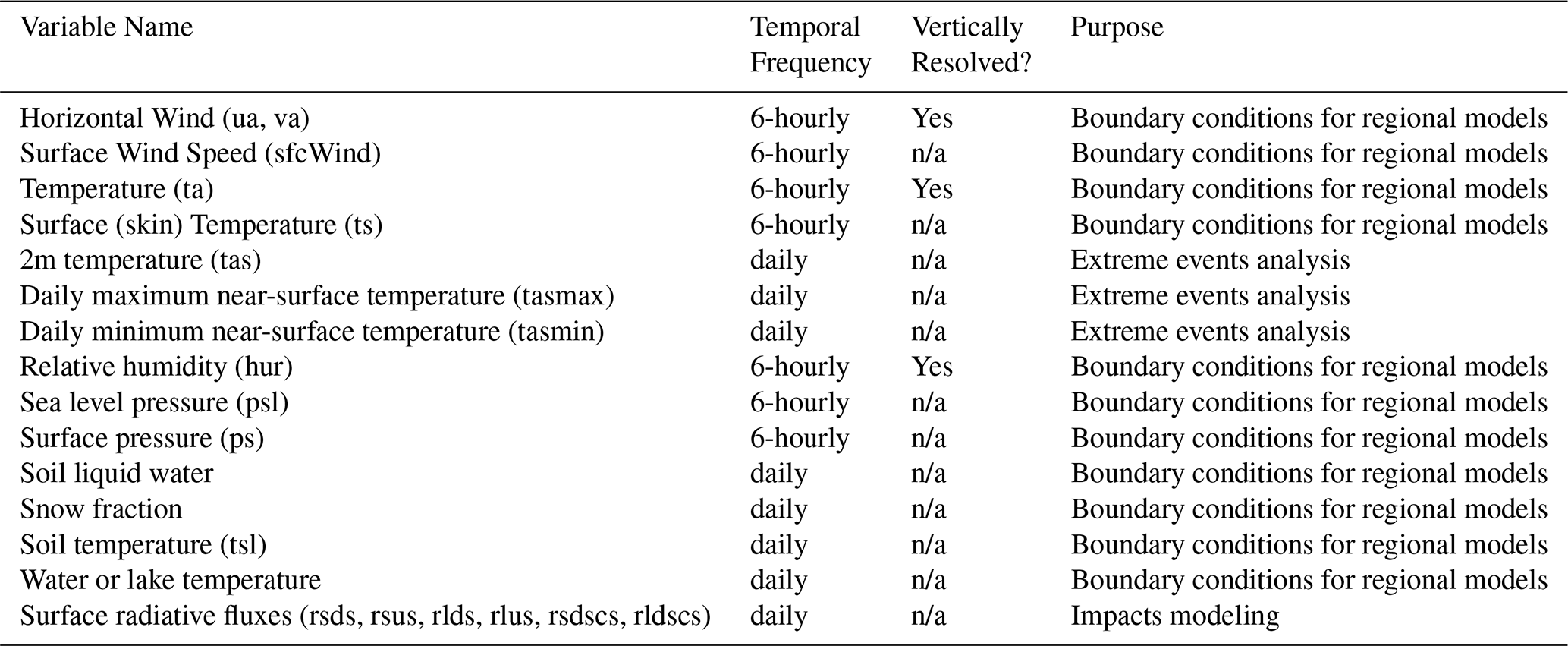
It will also be important for modeling centers to ensure their documentation for the models' versions used for GeoMIP experiments includes information related to components of the model necessary to understand the response to specific SRM methods (for instance, cloud microphysical schemes for MCB, CCT and MCT, details of the treatment of stratospheric aerosols for SAI), as part of the documentation required for the CMIP Rapid Evaluation Framework (REF) (Hoffman et al., 2026), as well as specific diagnostics that would enable a better validation of SRM-specific aspects (for instance, diagnostics from historical simulations with interactive volcanoes to enable comparison with observations, Quaglia et al., 2023) in order to make systematic benchmarking of the models used simpler (Hassler et al., 2026).

Required output for MCT experiments

Correctly attributing the MCT response requires cloud fields at higher temporal resolution than standard monthly means; in particular, monthly-mean bulk phase ratios are insufficient to reproduce satellite-based cloud-top phase climatologies stratified by temperature. In addition to the standard 2D monthly-mean fields from Level 0, the Level 1 protocol therefore requires:

• Daily sampled instantaneous values of 2D fields (TOA, ATM, and BOA clear-sky and all-sky radiative fluxes) and 3D temperature and cloud fields (cloud water content and particle number for liquid and ice; snow and rain if available);

• COSP forward-simulator output (CALIPSO/ISCCP diagnostics) for direct comparison with satellite cloud-top-phase retrievals;

• Glaciation process rates (daily sampled instantaneous values): at least heterogeneous droplet freezing rate, ice depositional growth rate (WBF), and ice/snow riming rate. Because daily 3D process rates are very expensive to store, we encourage the use of online 2D column-integrated, mixed-phase-integrated, and cloud-top alternatives, which will otherwise be calculated offline.

6 Conclusions

Earth system modeling of different SRM techniques has substantially grown our collective understanding of their potential to avert some consequences of anthropogenic global warming, as well as potential unintended consequences on other climate variables. With this, we do not claim that all questions have been answered; rather, an increased exploration of the size of the potential space of these interventions has shown that deep care should be taken in claiming that, generically, “SRM would do X to system Y”. Recent research has shown that how the specific SRM techniques are simulated, in terms of location, timing, underlying scenario, and magnitude of intervention, all matter when discussing the potential impacts, and while some broad consequences are independent of these details, many are not. Similarly, a renewed interest in the physical and ecological impacts, also driven by an expansion of the community of users for such simulations, has led to a deeper understanding of the sources of uncertainty in such simulations.

The GeoMIP community has found that the need to increase the exploration of the scenario space, the need to be able to pinpoint specific physical uncertainties and sources of inter-model spread, and the need to maintain a simple system that is usable and understandable by a broad set of users are all very relevant needs that must be balanced, and no perfect answer exists. The framework GeoMIP is proposing for CMIP7 tries to address many of these challenges, and has matured over many annual workshops with intense discussions. We have aimed to keep proposed experiments simple, yet plausible, to enable the community to both understand more easily sources of uncertainties while relying on a similar scenario framework as other MIPs. We have accompanied the main experiments with more simple experiments that are both useful for diagnosing responses and that can be potentially leveraged to build emulators that can accompany the main simulations to expand the scenario space beyond what is computationally feasible in ESMs. And, this time, we have also proposed a more flexible framework in which modeling teams can maintain a common basis and yet explore specific scenarios that are of interest to them. Simplicity is a deliberate choice, rather than the product of naivete. The main goal of GeoMIP remains that of highlighting sources of agreement and disagreement across different models, and that is undoubtedly easier to do in somewhat simplified modeling scenarios. This should not be taken (and indeed, the GeoMIP community has never done so) as a claim that the scenarios we produce are aiming to be prescriptive or predictive. A clearer understanding and disentangling of physical impacts has the potential to clarify the implications of what could be “real-world” deployments, which can serve as an input for other fields of research, as well as interdisciplinary research, to expand the space of assessment and understanding of risks beyond climate science (Tilmes et al., 2024; Beckage et al., 2025; Estrada et al., 2026).

Appendix A: Additional figures

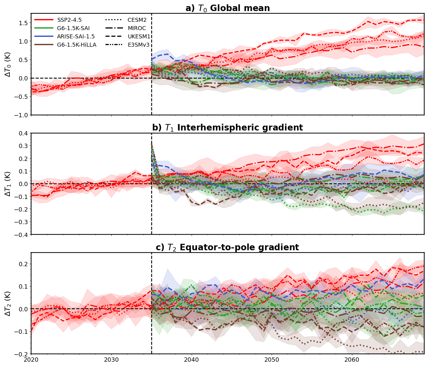
Figure A1 Evolution of (a) global-mean temperature T₀, (b) interhemispheric temperature gradient T₁, and (c) equator-to-pole temperature gradient T₂ from 2020–2069 for SSP2-4.5 (red) and SAI scenarios (G6-1.5K-SAI, green; ARISE-SAI-1.5, blue; HiLLA-SAI, brown). Line style denotes the climate model (CESM, MIROC, UKESM and E3SM) and line shading show the ensemble spread.

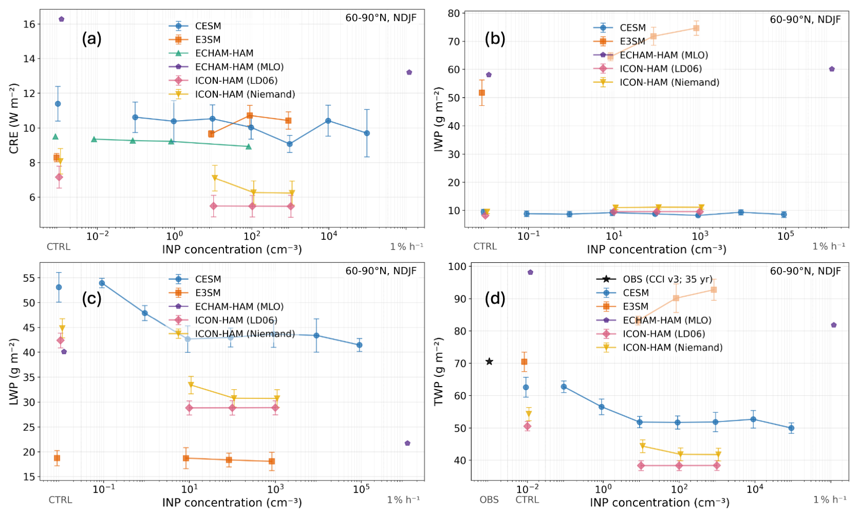
Figure A2 Arctic-mean (60–90° N) NDJF response as a function of INP concentration for all MCT-MIP Level 0 models and configurations. (a) Net cloud radiative effect (CRE, W m⁻²); the control value is shown at the left margin. (b) Ice water path (IWP, g m⁻²); E3SM's anomalously high and monotonically increasing IWP explains its warming CRE response. (c) Liquid water path (LWP, g m⁻²). (d) Total water path (TWP, g m⁻²). Error bars denote the inter-annual standard error of the mean.