Development of a high-resolution coupled SHiELD-MOM6-LM4 model – Part 2: Model overview, coupling technique, and evaluation of hydrological extremes during Hurricane Helene

This work describes the implementation strategy and technical challenges involved in integrating the Geophysical Fluid Dynamics Laboratory (GFDL)’s Land Model (LM4) with dynamic subgrid tiling capabilities within the atmospheric model, System for High-resolution modeling for Earth-to-Local Domains (SHiELD), capable of kilometer-scale global simulations. A key challenge addressed in this effort is coupling LM4, which was designed for implicit surface flux coupling, with SHiELD’s explicit physics solver. We achieve this through a refactoring of the atmospheric physics suite and code drivers, enabling implicit land-atmosphere coupling of heat and moisture within the well-established FMS coupler infrastructure. The resulting flexible architecture supports multiple model configurations from a single executable without recompilation. This extends SHiELD from an uncoupled atmospheric model, in which land processes are treated as a part of the atmospheric physics package, to a fully coupled high-resolution atmosphere-ocean-land-ice model. We demonstrate the new system through a high-resolution global simulation of Hurricane Helene's landfall where the land component realistically captures the rapid soil saturation, localized runoff generation and multi-day river flooding in Western North Carolina. These results demonstrate the technical coupling strategy, unlock new forecast capabilities, and highlight the importance of interactive land-atmosphere coupling for simulating extreme weather and hydrological events.

1 Introduction

Land–atmosphere interactions are now widely recognized as a fundamental source of predictability for hydroclimate extremes. Soil moisture anomalies persist for weeks to months and feed back onto the overlying atmosphere, and this land memory has been shown to modulate droughts, heatwaves, and heavy-precipitation events across a range of models and observational studies (Koster et al., 2004; Seneviratne, 2006; Miralles et al., 2019). Thus, representing these interactions has long been essential for seasonal and climate models, whereas short-range weather models have historically placed less emphasis on these processes. However, given that these models are now operating at very high resolutions, interest in simulating extreme hydrological events has risen. On shorter timescales, particularly during tropical cyclones landfalls, the land surface is not simply a passive recipient of atmospheric forcing: antecedent soil saturation, infiltration capacity, and drainage efficiency directly govern the magnitude, timing, and spatial extent of inland flooding, as illustrated by Hurricane Helene's impact on Western North Carolina in 2024. Realistically representing this two-way exchange, rather than treating the land as a passive lower boundary condition, is therefore central both to short-range prediction of hydrological extremes and to Earth system prediction more broadly.

Several operational and research Earth system models have adopted different strategies to represent these land–atmosphere interactions and integrate hydrological processes. At ECMWF, the Integrated Forecasting System (IFS) couples its atmospheric model to the Carbon-Hydrology Tiled ECMWF Scheme for Surface Exchanges over Land (CHTESSEL/ECLand) (Balsamo et al., 2009) as one component of a single-executable, multi-model coupling strategy that also includes ocean, sea ice, and wave models (Boussetta et al., 2021; Mogensen et al., 2012; Roberts et al., 2018). The atmosphere and land components are implicitly coupled following the pioneering work of Best et al. (2004). River discharge and flood inundation, however, are not solved prognostically within IFS itself; runoff is instead passed one-way to external routing models such as LISFLOOD in the Global Flood Awareness System (GloFAS) or CaMa-Flood, which diagnose streamflow and inundation offline from the land-surface runoff (Alfieri et al., 2013; Yamazaki et al., 2011). NOAA's Unified Forecast System (UFS) takes a related but distinct approach, coupling the FV3 dynamical core to the Noah-MP land surface model through the Common Community Physics Package (CCPP), with inter-component exchange handled by the Community Mediator for Earth Prediction Systems (CMEPS), built on the NUOPC/ESMF interoperability layer (Worthen et al., 2024). The UFS, also, does not simulate river discharge and flooding prognostically, but provides precipitation data to an external hydrological model, the National Water Model (Cosgrove et al., 2024). Efforts are also underway to couple the UFS model to LM4 itself; though this coupling will be explicit given the constraints of the CMEPS coupler framework. Finally, NCAR's Community Terrestrial Systems Model (CTSM), built around the Community Land Model version 5 (CLM5) (Lawrence et al., 2019), is designed to couple to a variety of host atmospheric models, including models such as WRF, through the Lightweight Infrastructure for Land–Atmosphere Coupling (LILAC) (UCAR, 2020), separating land model development from any single atmospheric host.

Building on decades of modeling advances in weather forecasting and subseasonal prediction at the Geophysical Fluid Dynamics Laboratory (GFDL), the System for High-resolution modeling for Earth-to-Local Domains (SHiELD) (Harris et al., 2020; Zhou et al., 2024) is being progressively extended from a typical atmospheric general circulation model toward a complete Earth System configuration capable of capturing oceans, land surface water dynamics, vegetation, and biogeochemical interactions. A first step toward this goal, Mouallem (2024) incorporated the Flexible Modeling System (FMS) full coupler infrastructure into SHiELD, providing the framework required for component-based Earth System coupling. Building upon this capability, Mouallem et al. (2025) established the atmosphere-ocean coupling framework by integrating SHiELD with the Modular Ocean Model version 6 (MOM6). This work demonstrated the technical viability of coupling a regional, kilometer-scale hurricane model with a comprehensive ocean model in both an idealized test case and a simulation of Hurricane Helene (2024), enabling two-way, high-resolution air–sea interactions. In that configuration, the atmosphere was initialized from GFS analysis and the ocean from GLORYS reanalysis, while land processes remained embedded within the atmospheric physics suite, with turbulent and radiative exchanges simulated by the Noah land surface model (Ek et al., 2003). Although this configuration enabled high-resolution atmosphere–ocean interactions, it lacked an interactive land component capable of representing detailed soil hydrology, vegetation dynamics, and prognostic river processes required for simulating land-surface responses to extreme precipitation events.

The present work closes this gap. Distinct from the approaches described above, it adopts a fully integrated coupling strategy in which the atmosphere, ocean, sea ice, land, and river routing are all coupled through the Flexible Modeling System (FMS) infrastructure. Unlike previous SHiELD configurations, LM4 and SIS2 are treated as independent Earth system components and coupled implicitly with the atmosphere, while river runoff and discharge are simulated prognostically within the same framework. This development extends the regional atmosphere-ocean only configuration of Mouallem et al. (2025) to a full global atmosphere-ocean-ice-land system providing the foundation for high-resolution Earth system forecasting and prediction. Achieving this, however, was not straightforward: LM4 and SIS2 were originally designed for implicit surface flux coupling within GFDL's broader modeling infrastructure, whereas SHiELD's atmospheric physics solver is explicit. Reconciling the two required a substantial refactoring of the atmospheric physics suite and model drivers, ultimately yielding an implicit coupling strategy for both the land and ice components within the established FMS coupler framework. Together, this refactored coupling strategy brings qualitatively new capabilities to SHiELD. SHiELD shares the same FV3 dynamical core and FMS infrastructure as the broader GFDL family of atmospheric models, and because its atmospheric physics suite and initialization are drawn from the operational Global Forecast System (GFS), SHiELD's atmosphere is functionally analogous to that of GFS. In place of the previously embedded Noah scheme, an implicit coupler now connects LM4 and SIS2 to the atmosphere as independent Earth system components (sea ice coupling via SIS2 is detailed in a companion paper; the present paper focuses on the land component, LM4). The resulting configuration bridges GFDL's weather-forecasting and decadal-to-centennial Earth system modeling capabilities, reconciling meteorological, hydrological, and ecological processes across multiple scales. This reconciliation plays a critical role in forecasting and predicting complex hydroclimate phenomena.

LM4 provides a comprehensive treatment of soil hydrology across multiple layers with explicit subsurface water flow, freezing and thawing dynamics, surface and subsurface runoff generation, river routing, snow physics, and dynamic vegetation processes. These capabilities are essential for realistically simulating the land surface response to extreme precipitation events, the evolution of soil moisture and its memory on subseasonal timescales, and the feedbacks between land state evolution and atmospheric dynamics. For coupled high-resolution forecasting applications, the inclusion of a prognostic river routing scheme is particularly impactful: it enables the simulation of downstream flood propagation over multi-day timescales following extreme precipitation, a capability entirely absent in the prior configuration.

In parallel, this work advances the SHiELD software architecture through a flexible and modular design that supports multiple coupled configurations from a single source code and executable without recompilation. This “one code, one executable, one workflow” philosophy, consistent with the broader SHiELD development strategy, facilitates controlled experimentation, ensures backward compatibility with prior configurations, and streamlines the path toward operational deployment.

We demonstrate the new system through a fully coupled global simulation of Hurricane Helene's landfall in September 2024, an exceptionally demanding and scientifically relevant test case. Helene produced catastrophic flooding in Western North Carolina driven by extreme orographic precipitation interacting with steep terrain and rapidly saturating soils, a scenario that simultaneously stresses the atmospheric dynamics, land surface hydrology, and river routing components of the model. The simulation reveals that the coupled system realistically captures rapid soil saturation, localized runoff generation concentrated in the southern Appalachians, and multi-day river flooding.

The remainder of the paper is organized as follows. Section 2 describes the primary model components. Section 3 describes the coupling methodology including physical processes, implicit coupling and code refactoring. Section 4 presents a high-resolution global simulation and examines the land component’s response following the landfall of Hurricane Helene in September 2024. Section 5 illustrates a key advantage of the fully coupled global model by successfully capturing two extreme independent catastrophic events in one simulation.

2 Model Primary Components

The main model components follow those described by Mouallem et al. (2025), with the addition of GFDL's land model LM4. We briefly introduce these components here.

2.1 LM4 Land component

The land component is GFDL's Land Model version 4 (LM4.0), a comprehensive land surface model designed to simulate the physical, biological, and chemical processes governing land-atmosphere interactions (Zhao et al., 2018; Held et al., 2019). LM4 represents a significant advancement over its predecessors, incorporating detailed treatments of land surface heterogeneity, soil hydrology, river hydrology, snow physics, and carbon cycling. The model simulates soil hydrology using multiple soil layers with explicit representation of subsurface water flow, freezing and thawing processes. LM4 also incorporates a dynamic vegetation component that captures the evolution of surface and vegetation properties (e.g. leaf area index, biomasses, height, surface roughness), processes (e.g. photosynthesis, transpiration and vertically-resolved water uptake from soil, interception of precipitation) and their responses to climate variability, making it particularly well-suited for long-term climate and Earth system modeling applications.

For the purposes of short-term high-resolution prediction modeling explored here, the hydrological and snow modeling capabilities are of most interest. Therefore, biogeochemical cycling and vegetation dynamics are disabled for efficiency and simplicity. However, all LM4 capabilities are available within SHiELD for activation when a scientific need arises.

2.2 SHiELD Atmosphere component

The atmospheric component is the System for High-resolution modeling for Earth-to-Local Domains (SHiELD) (Harris et al., 2020), a nonhydrostatic model using the GFDL Finite-Volume Cubed-Sphere Dynamical Core FV3 (Lin and Rood, 1996, 1997; Lin, 2004; Putman and Lin, 2007; Harris and Lin, 2013; Chen et al., 2013; Harris et al., 2016; Mouallem et al., 2022, 2023; Santos et al., 2025) and heavily upgraded physics parameterizations, originally adopted from the Global Forecast System (GFS). Currently, we use the GFDL microphysics scheme version 3 (Zhou et al., 2022b), the Eddy-Diffusivity Mass-Flux (EDMF) boundary layer scheme (Han and Bretherton, 2019), and the scale-aware Simplified Arakawa-Schubert (SAS) convection scheme (Han et al., 2017). For the standalone uncoupled SHiELD configuration, we use the Noah Land Surface Model (Ek et al., 2003) or Noah-MultiParameterization (Niu et al., 2011) and a modified version of the Mixed Layer Ocean of Pollard et al. (1973).

2.3 MOM6-SIS2 Ocean and sea ice component

The ocean and sea ice components employ the Modular Ocean Model version 6 (MOM6) and the Sea Ice Simulator version 2 (SIS2), developed at GFDL (Adcroft et al., 2019). MOM6 employs a finite-volume approach on a C-grid, enabling conservation of mass, heat, and tracers while allowing for flexibility in resolving complex oceanic features, such as boundary currents, mesoscale eddies, and thermohaline circulations. MOM6 is highly configurable, supporting applications ranging from idealized studies to high-resolution global simulations and earth system models. SIS2 complements MOM6 by simulating the dynamics and thermodynamics of sea ice, including ice growth, melt, deformation, and ridging processes. It incorporates advanced parameterizations to capture the essential feedback mechanisms between sea ice, ocean circulation, and atmospheric forcing. The details of ocean configuration follow that of SPEAR-HI and will not be repeated here for brevity.

2.4 FMS Infrastructure layer

The Flexible Modeling System (FMS) (Balaji, 2012; Balaji and Langenhorst, 2012) serves as the infrastructure layer underlying GFDL models. It provides a software environment designed for the efficient development, construction, and execution of atmospheric, oceanic, and climate models written in Fortran (and now DSL and Python) for high-performance computing systems. FMS includes MPI domain decomposition for scalable parallel computations, standardized interfaces between component models, and tools for I/O, time-stepping orchestration, and data exchange between model grids. By insulating users from machine-specific details and supporting both distributed and shared memory architectures, FMS enables scientific groups to simultaneously develop new physics and algorithms within a coordinated and collaborative framework.

3 Coupling methodology

3.1 Physical processes

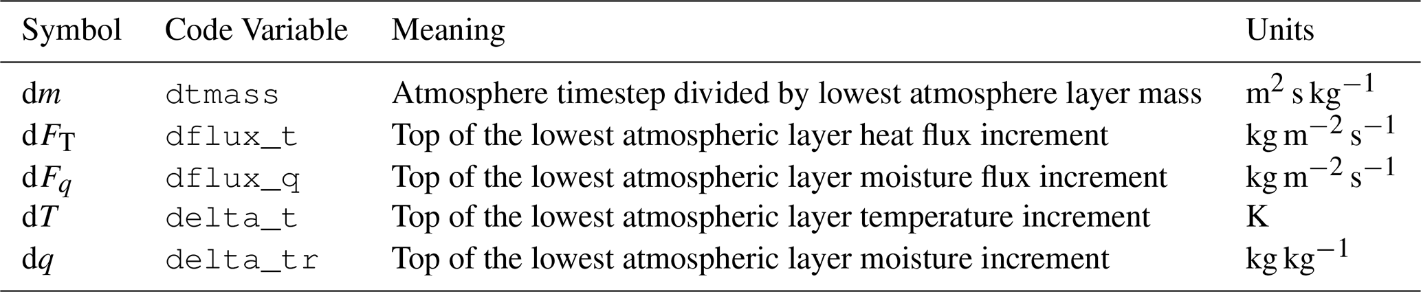
As described in Mouallem et al. (2025), any variable or parameter can be projected between the native grids of a model component and the exchange grid. In the present configuration, a set of dynamic and physical variables from the atmosphere, land and ocean components are mapped onto the exchange grid (called Xgrid hereafter for brevity) where interface quantities are computed and then projected back to each component as shown in Fig. 1. The general exchange between the ocean, atmosphere and the Xgrid follows that described in Mouallem et al. (2025). Here we additionally include the land component in the exchange workflow to obtain a fully coupled atmosphere-ocean-land model. Atmospheric state variables and radiative fluxes are first projected onto Xgrid, as well as land and ocean surface properties to compute surface fluxes of momentum, heat, and moisture. These fluxes are then mapped back to the corresponding component grids to update their surface boundary conditions. Variables highlighted in green denote the subset of atmospheric variables required to support implicit coupling with the land component. These fields enable a consistent formulation of surface exchange variables to solve the vertical diffusion equation (in the atmosphere mostly eddy diffusivity from the planetary boundary layer scheme) and tendencies for land-atmosphere implicit coupling. This is described in the next section.

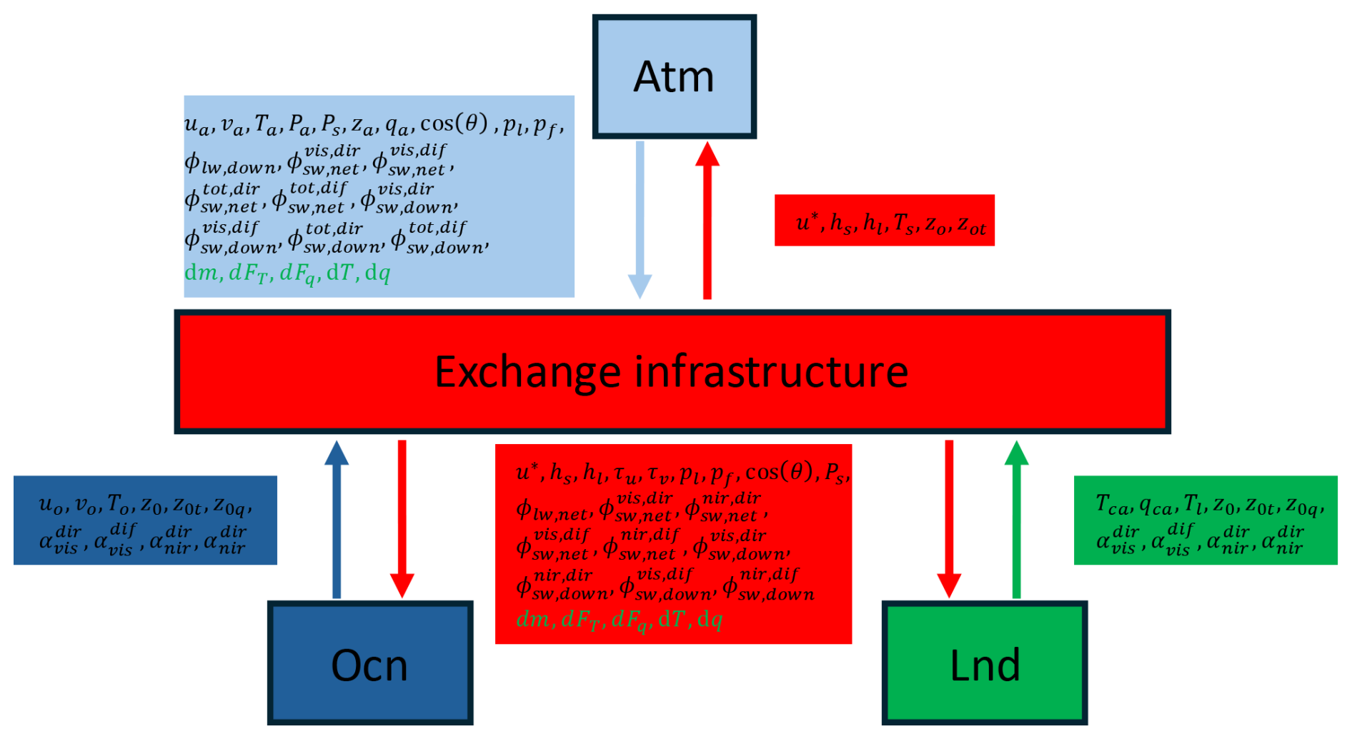
Figure 1 Key variables exchanged through the atmosphere, exchange grid, ocean (including sea ice) and land components. Variables are described in Tables 1 and 2.

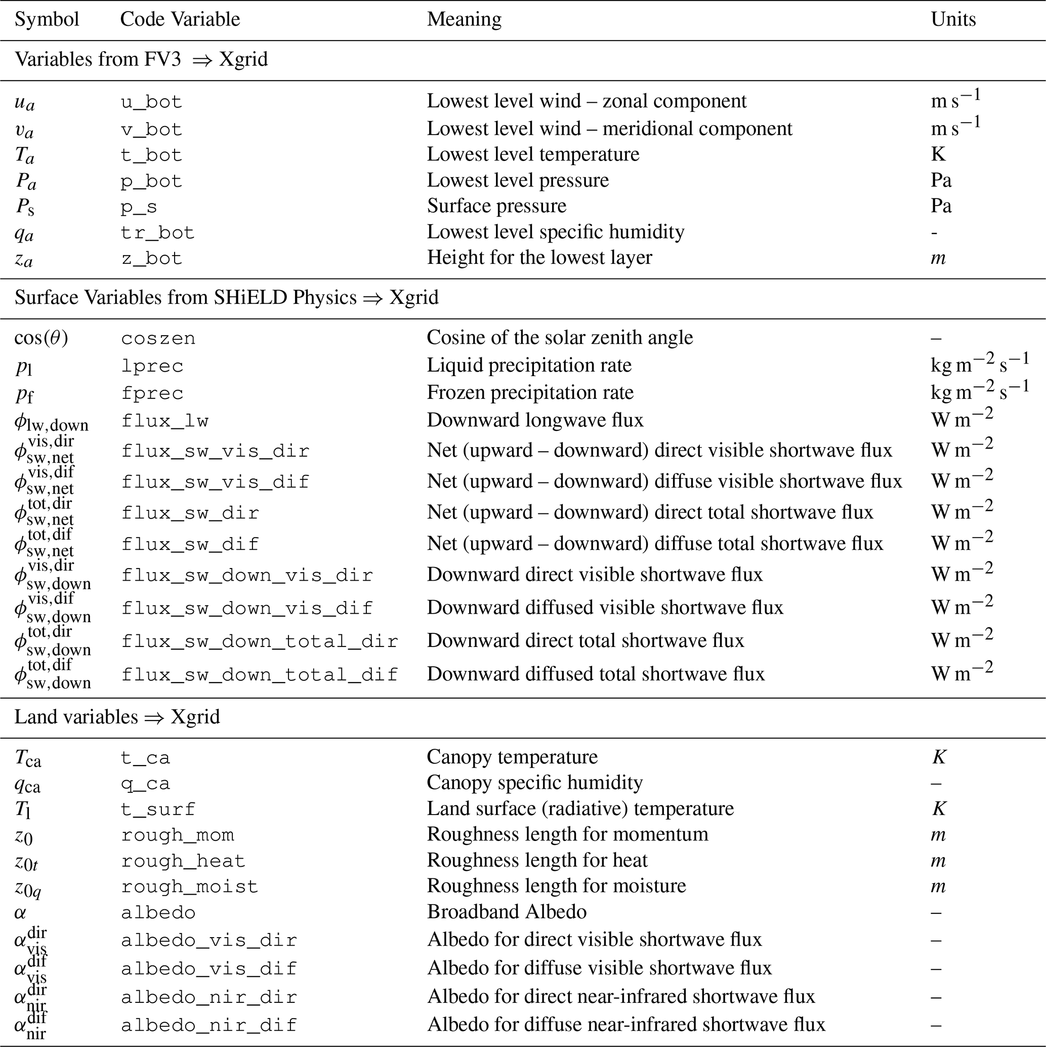
Tables 1 and 2 detail the atmosphere and land related variables projected onto the exchange grid shown in Fig. 1. Atmospheric variables are grouped into two categories: dycore variables, comprising the lowest-level wind components, surface pressure, temperature, layer height, and tracer fields (if present); and physics variables, comprising shortwave and longwave radiation fluxes, liquid and frozen precipitation rates, and the cosine of the solar zenith angle. Land variables include surface parameters such as radiative and canopy air temperature, surface specific humidity, albedo for direct and diffuse shortwave fluxes, and roughness length scales for momentum, heat, and moisture.

Table 1 Summary of the key atmosphere and land variables projected onto the Xgrid. Atmosphere variables are categorized into dynamic variables (output from the FV3 dynamical core) and physics variables (surface-level outputs from the physics suite).

Land implicit coupling

Figure 2 presents a schematic representation of two alternative coupling strategies employed to solve the vertical diffusion equation across the land–atmosphere interface. In both panels, the vertical discretization is depicted as a series of horizontal layers indexed by k, with the land surface prescribed as the lower boundary condition.

The explicit coupling scheme (left panel) employs a sequential approach. Here, the atmospheric vertical diffusion, computed implicit-in-time to ensure numerical stability, results in a tridiagonal matrix which is solved first (Arrow 1), typically using surface fluxes (heat, moisture) calculated from the state of the land surface at the previous time step (t). The tridiagonal solver performs both its downward and upward sweeps independently of the current land surface update. Next, the land surface model advances its state (Arrow 2) using the updated lowest layer atmospheric variables as forcing. In this process, the canopy or first soil layer is updated first (first small arrow in Arrow 2), followed by the soil heat diffusion solver, and then the canopy temperature is updated again. In the explicit scheme, the lagging of the lower boundary condition decouples the mathematical solution of the turbulent transport between land and atmosphere, which can introduce inconsistencies between the surface fluxes and the atmospheric state, potentially degrading numerical stability at longer time steps.

On the other hand, the implicit scheme avoids this inconsistency by integrating the land surface directly in the atmospheric tridiagonal solver as a single extended column. The atmospheric downward pass runs from the top of the atmosphere down to the land surface (Arrow 1), after which the land surface solver is called (Arrow 2). Consequently, the relationship between surface fluxes and land surface is linearized and the lowest atmosphere layer and land surface are solved simultaneously. Finally, the atmosphere upward sweep propagates from the updated surface to the top of the atmosphere (Arrow 3). It is worth mentioning that implicit coupling also applies to the ice component which is advanced in the fast loop of the solver as shown later. The ocean will stay explicitly coupled to the atmosphere.

Table 2 Summary of additional variables needed for atmosphere and land variables implicit coupling (shown in green in Fig. 1).

In the current implementation, the friction velocity (u_*) is computed in the Monin–Obukhov Similarity Theory (MOST) scheme and held constant during the implicit solution for temperature and moisture. As a result, the exchange coefficients remain explicit, while the heat and moisture fluxes are treated implicitly. This design follows the existing atmospheric surface-layer implementation in Earth System Model 4 (ESM4) and avoids introducing additional dependencies while maintaining consistency of the resulting fluxes throughout the implicit iteration. This logic is consistent with the algorithm introduced in Held (2004). This approach is applied only to temperature and moisture in the current implementation. The same approach could be extended for momentum and other tracers; however, we assume that surface fluxes of momentum and other tracers have no implicit dependence on surface parameters. Implicit momentum coupling may become important in future implementation for higher resolution configurations to simulate landslides where the no slip boundary condition is no longer valid.

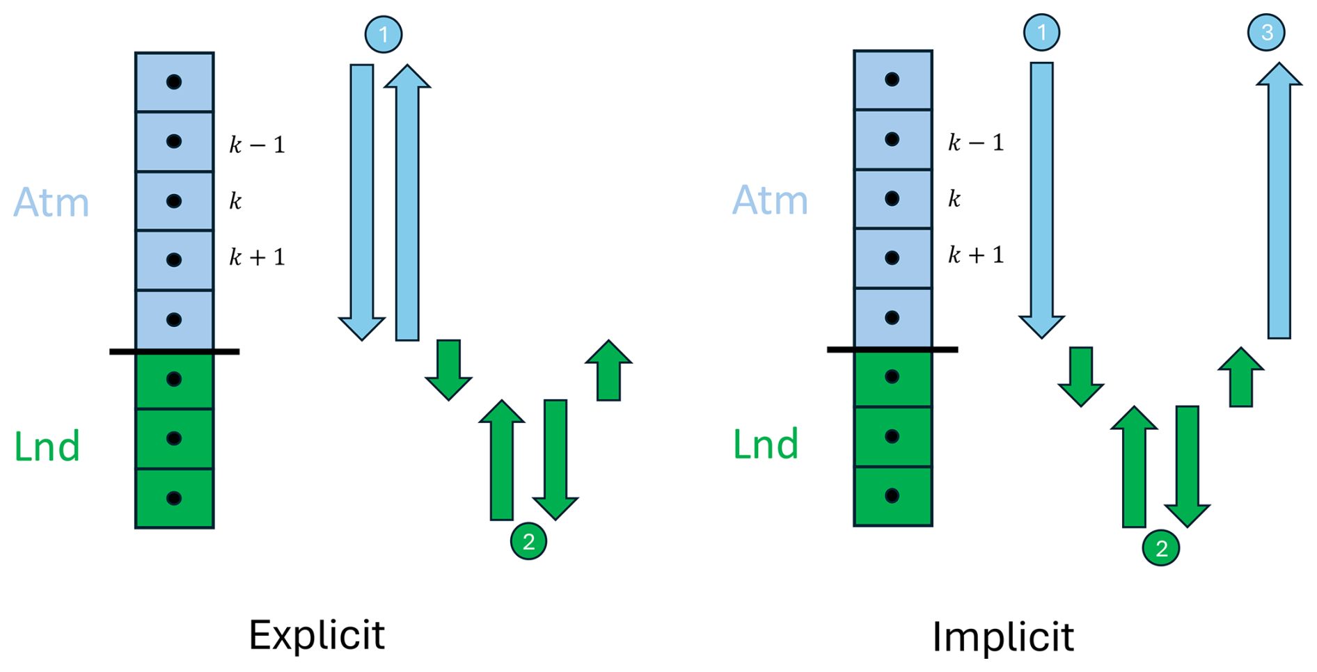
Figure 2 Schematic of explicit (left) and implicit (right) coupling schemes for vertical diffusion across the land–atmosphere interface. Arrows indicate the sequence of atmospheric and land surface tridiagonal solver sweeps within a single time step.

3.2 Software framework and code refactoring

Figure 3 illustrates a schematic of a 1D exchange grid for a full atmosphere, ocean and land coupled model. Analogous to the projection of near-surface atmospheric and oceanic state variables onto the Xgrid in Mouallem et al. (2025), land surface variables and parameters are now likewise projected onto the exchange grid. On the Xgrid, surface fluxes of momentum, heat, moisture, and radiation are diagnosed using land‐specific surface properties (e.g., roughness lengths, albedo, and surface temperature and humidity) and are subsequently remapped to the atmosphere and land component grids. This extension allows the land–atmosphere interface to be treated consistently with the ocean–atmosphere interface, while maintaining the same conservative and modular coupling strategy. The coupling frequency remains user-configurable and subject to the constraints discussed in Part 1.

An important feature illustrated in Fig. 3 is that a single atmospheric grid cell can geometrically overlap both the land and ocean grids, as shown by the vertical dashed lines. In such cases, the atmospheric grid cell is associated with multiple exchange grid cells, each corresponding to the area of intersections between atmospheric cells and the land and ocean component grid cells (Balaji et al., 2006). On the land and sea ice side, the Xgrid cells can be further subdivided dynamically to represent inherent heterogeneity of the surface, such as area fractions of lakes, glaciers, croplands, and forests in the land grids, and different thickness categories of the sea ice. All flux computations are performed on this Xgrid representation. Since surface fluxes from the land and ocean depend nonlinearly on the atmosphere and surface properties, they are evaluated independently over their respective Xgrid areas and are subsequently area-averaged when remapped to the atmospheric grid. Similarly, atmospheric fields are consistently distributed to the land and ocean components according to the same geometric decomposition. This prevents or greatly minimizes numerical discontinuities between different components at the coastlines.

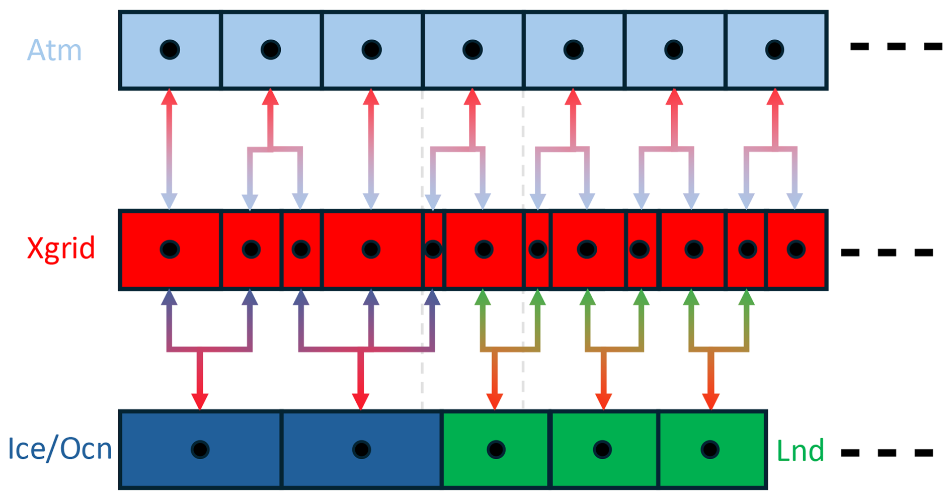
Figure 3 Schematic of a one-dimensional exchange grid and communication map between the atmosphere, land and ice components at different resolutions. The red side of the arrow indicates where variables are projected from the exchange grid. The light-blue, dark blue and green sides of the arrow represent the projection of variables to the exchange grid from the atmosphere, ice or land components, respectively.

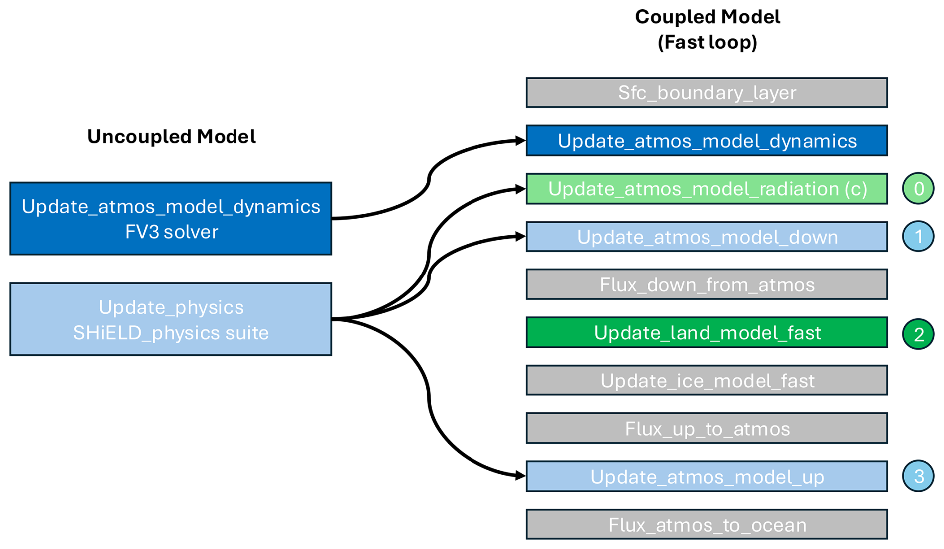
Figure 4 Schematic of the code structure of the uncoupled and coupled models. Arrows show the uncoupled components that are refactored in the coupled call sequence.

Figure 4 illustrates the structural refactoring of the model required to transition from the uncoupled configuration to the coupled model's “fast loop” of the FMS full coupler. The left panel depicts the legacy uncoupled model which encapsulates the time-stepping into two primary high level drivers:

• Dynamics: update the dynamics using the dynamical core FV3

• Physics: compute the physics tendencies from SHiELD's physics parameterization suite

The right panel details the fast loop of the coupled model, demonstrating how the monolithic calls are decomposed and reordered to facilitate tighter coupling between different model components. As indicated by the arrows, the dynamics component maps directly to the dynamic update call within the coupled sequence. The physics component is split into three distinct phases (0-1-3) allowing tighter coupling with land and ice. The execution sequence proceeds as follows:

• Sfc_boundary_layer: compute explicit fluxes and their derivatives at the surface boundary

• Update_atmos_model_dynamics: update the dynamics using the dynamical core FV3

• Update_atmos_model_radiation: compute radiation tendencies

• Update_atmos_model_down: calculate the necessary atmospheric states to drive surface processes. This is where the downward sweep of heat and moisture is computed for implicit coupling.

• Flux_down_from_atmos: compute fluxes and derivatives corrected for implicit coupling.

• Update_land_model_fast: perform the land model fast time integration loop

• Update_ice_model_fast: perform the ice model fast time integration loop

• Flux_up_to_atmos: correct the flux given the updated land and ice variables

• Update_atmos_model_up: perform the upward sweep of the heat and moisture and all the remaining physics updates.

• Flux_atmos_to_ocean: correct fluxes of some fields to be passed to the ocean.

Figure 5 illustrates the code structure for the uncoupled and coupled models. In the uncoupled model, the dynamics are called first for a timestep dt_atmos. The updated solution is then passed to the physics parameterizations where all physics tendencies are computed and used later on to update the model state. As implied by the schematic, all the physics parameterization are computed, in bulk at this stage including:

1. Surface layer and surface energy balance (over land, ocean, and sea-ice), including turbulent exchange coefficients, near-surface diagnostics, and land/sea-ice model updates.

2. Planetary boundary layer (PBL) vertical mixing, providing turbulent transport of momentum, heat, moisture and other tracers.

3. Orographic and convective gravity-wave drag as well as Rayleigh damping, which modify momentum and temperature.

4. Radiative heating (shortwave and longwave), passed from the radiation scheme and applied at the physics timestep.

5. Ozone and stratospheric water-vapor chemistry tendencies.

6. Shallow and deep convection (based on mass-flux parameterizations), including convective heating, transport and detrainment of tracers, and convective precipitation.

7. Cloud microphysics, including large-scale condensation/evaporation and precipitation processes.

8. Diagnostic routines, including precipitation type, land-surface adjustments, and calculation of precipitation, cloud fraction, cloud water/ice, and near-surface fields.

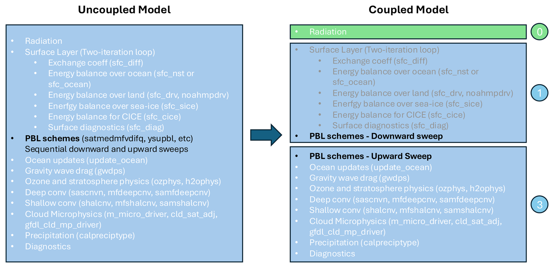
Figure 5 Schematic of the time-integration sequence in the uncoupled (left) and coupled (right) SHiELD configurations. The arrows highlight the refactored structure of the physics suite. Grey text denotes the SHiELD_physics surface layer flux computation, which is enabled in the uncoupled configurations and disabled for the coupled configurations.

Figure 5 also details the internal restructuring of the physics suite required to support the coupled configuration including land implicit coupling. The refactoring process consists of splitting this monolithic structure into different components as described in Fig. 4 to have a radiation module, a surface and downward physics step and lastly, an upward and moist processes step. The right panel illustrates the new refactored structure. Radiation routines (step 0) are now split and called separately. Step (1) corresponding to Update_atmos_model_down contains the uncoupled surface flux calculations, the downward sweep of the tridiagonal matrix for heat and moisture. Step (3) corresponding to Update_atmos_model_up contains the remaining physics calls. It is important to note that the momentum and the turbulent kinetic energy (TKE) upward and downward sweeps are still explicit in Update_atmos_model_down.

3.3 Flexible Surface-Coupling Architecture and Surface Flux Pathways

It is important to make the distinction between the surface layer calculation in sfc_boundary_layer shown in Fig. 4 and those shown as grey text in Fig. 5. The former represents surface fluxes at the coupler level, computed on the Xgrid between the atmosphere and ice/ocean components, as well as between the atmosphere and land components. In contrast, the latter surface layer calculation in update_atmos_model_down corresponds to fluxes produced internally by the atmospheric physics when interacting with embedded surface representation, such as the mixed-layer ocean and the NOAH or NOAH-MP land models. These internal flux computations are enabled for uncoupled model configurations and disabled for coupled configurations through Xgrid.

The current framework allows running different model configurations from a single source code and executable, without requiring recompilation. Following the “one code, one executable, one workflow” design philosophy, figure 6 illustrates the flexible surface-coupling software architecture allowing different coupled configurations to be set up from a common set of model components. The configurations differ in the complexity of their surface boundary components and the pathways of surface fluxes. The baseline uncoupled SHiELD configuration couples FV3–SHiELD_physics to null ocean and null land/ice components, providing a simple atmosphere-only (simple land and ocean are embedded in the physics) framework bypassing the exchange grid infrastructure. The SHiELD-MOM6 configuration replaces the null ocean/ice components with the MOM6/SIS2 ocean and sea-ice models, enabling two-way atmosphere–ocean–ice coupling while retaining a null land component. The SHiELD-LM4 configuration introduces the LM4 land model in place of the null land component but retains null ocean and ice components, allowing for interactive land–atmosphere coupling without a dynamic ocean. Finally, the SHiELD-MOM6-LM4 configuration is the most complete, coupling FV3–SHiELD_physics simultaneously to MOM6, SIS2, and LM4, thus representing a fully coupled atmosphere–ocean–sea ice–land system. The three latter configurations will invoke the exchange grid infrastructure. This modular architecture enables seamless switching between configurations via runtime namelist settings, without requiring recompilation of a new executable. In this context, it is worth elaborating on the null components. The null components act as passive placeholders that enable consistent coupling infrastructure without introducing additional physics or state evolution. Their primary role is to satisfy the interface requirement of the full coupler when a given component is absent or deactivated, by providing dummy routines and state variables necessary for the full model compilation and execution.

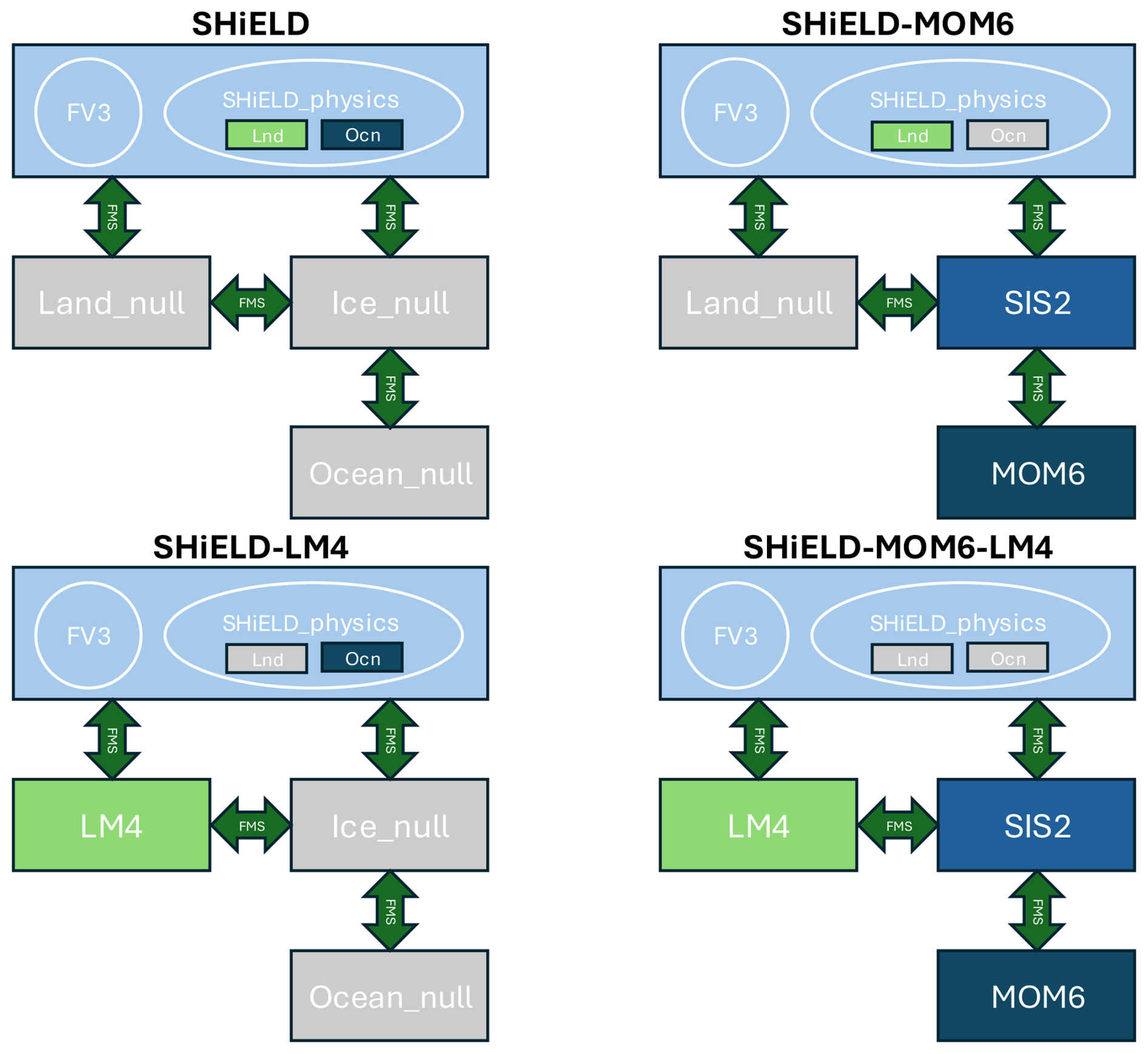
Figure 6 Schematic of different uncoupled and coupled model configurations. Land and ocean grid points are updated either by simplified surface schemes within the SHiELD physics suite or by fully interactive component models (e.g., MOM6 or LM4) coupled through the FMS coupler.

4 Simulations

We perform fully coupled global simulations using the SHiELD-MOM6-LM4 modeling system as presented in Fig. 6. The atmospheric component is the SHiELD v2022 configuration (Zhou et al., 2022a, b) which uses a C768 cubed-sphere grid, corresponding to a quasi-uniform horizontal resolution of approximately 13 km. The land model configuration, adopted from SPEAR-HI (Delworth et al., 2020), is using a C384 grid, corresponding to a global resolution of roughly 25 km. Given that we are focusing on the land model response and the hurricane is initialized right when it hits the coast with minor atmosphere-ocean interaction, we employ a coarse resolution one-degree ocean configuration on the tripolar grid with grid refinement to $\mathrm{1}/\mathrm{3}$° near the Equator, also taken from SPEAR. Two atmospheric initialization times are used across the experiments presented in this study. For the model–observation and coupled–uncoupled comparison in Fig. 7, the atmosphere is initialized from the GFS analysis at 00:00 Z on 26 September 2024, roughly 24 h prior to Helene's landfall, so that the simulated track and precipitation span the full 48 h period used for comparison against Stage IV (26 September 00:00 Z–28 September 00:00 Z) and capture the storm's approach through the Gulf of America, landfall, and inland propagation within a single continuous forecast. For all subsequent experiments examining the land surface response (Figs. 8–15), the atmosphere is instead initialized at 00:00 Z on 27 September 2024, coincident with Helene's landfall along the Florida coast. This later initialization was chosen to minimize the accumulation of track and intensity error over the open Gulf and to focus the analysis specifically on the land response during and after the storm's passage over land, rather than on the simulation's fidelity prior to landfall. The land and ocean initial conditions are not initialized from a separate spin-up performed specifically for these experiments. Instead, both components are initialized from an existing long-term SPEAR simulation that has already reached equilibrium under SSP2-4.5 radiative forcing (O'Neill et al., 2016; van Vuuren et al., 2014). Initial conditions are taken from the model state on 1 September 2024, providing physically consistent soil moisture, soil temperature, vegetation, snow, and ocean states representative of the September climatological season. Our objective is to capture the land response to this extreme atmospheric forcing rather than to reproduce the exact underlying land state. These climatologically representative initial conditions are sufficient for isolating the impact of the extreme atmosphere forcing and its effect on land. The fully coupled SHiELD-MOM6-LM4 system is integrated for three days. In this configuration, surface fluxes exchanged between the atmosphere, land, and ocean are computed and passed exclusively through the full FMS coupler. As a result, the atmospheric model receives land and ocean surface fluxes from the coupled land and ocean components, rather than from the internal parameterizations in the SHiELD physics suite (SHiELD_physics), and vice versa. This is described in Sect. 3. The primary objective of these simulations is to evaluate the land coupling framework and the land component response to atmosphere forcing.

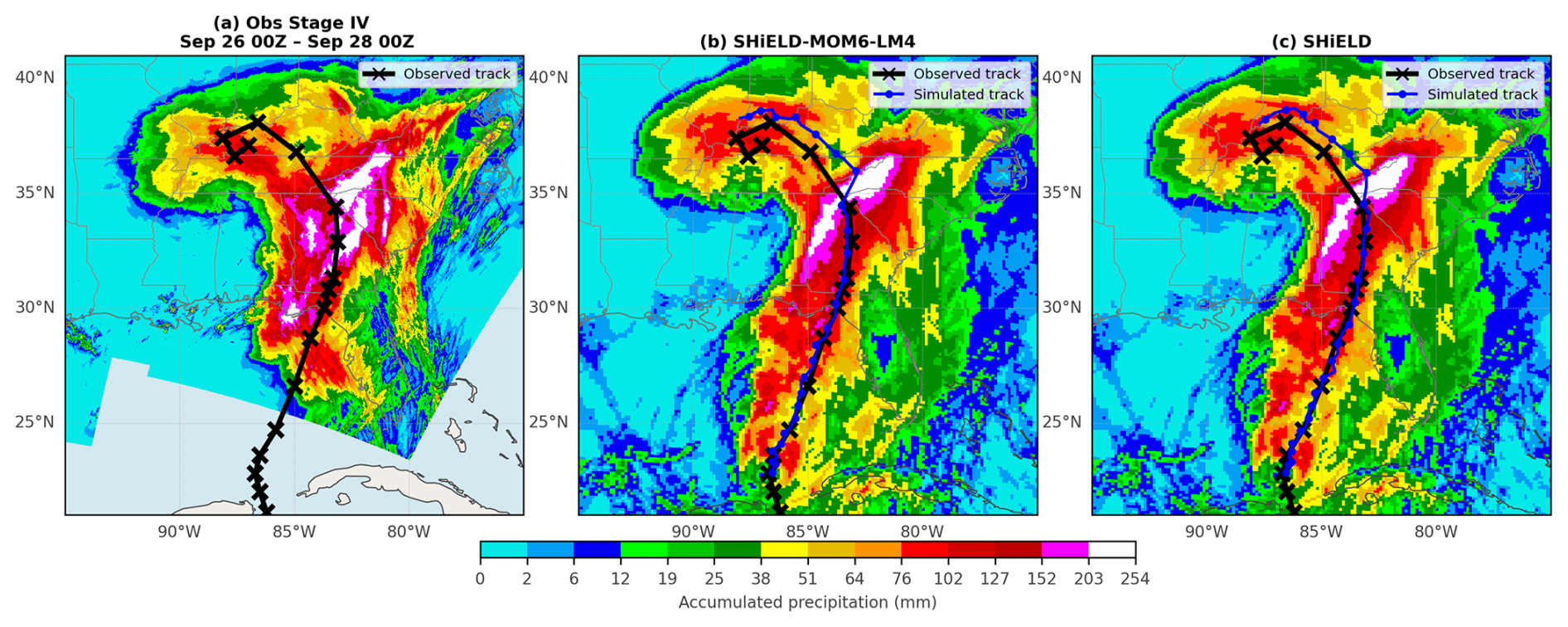
Figure 7 Accumulated precipitation (mm) for the period 26 September 00:00 Z–28 September 00:00 Z during Hurricane Helene, from (a) NCEP Stage IV multi-sensor observations, (b) the coupled SHiELD–MOM6–LM4 configuration, and (c) the uncoupled, atmosphere-only SHiELD configuration. The observed storm track (black, x-marker) is shown in all three panels; the corresponding simulated tracks (blue, circle marker) are overlaid in (b) and (c).

To evaluate whether the introduction of interactive land–atmosphere coupling and the choice of land initial conditions influence the simulated evolution of Helene, we compare accumulated precipitation and storm track between the coupled SHiELD–MOM6–LM4 configuration and an uncoupled, atmosphere-only SHiELD simulation initialized from the same GFS analysis in Fig. 7. Both configurations reproduce the essential features of the observed event well when compared against Stage IV observations. Heavy precipitation extends from the Gulf, to Georgia then North Carolina and finally tilted eastward. The location of extreme rainfall (>150 mm) over the Appalachian region in NC where the catastrophic flooding occurred is apparent and well captured in the simulation in both model configurations. More importantly for the present study, the coupled and uncoupled simulations are nearly indistinguishable in both track and accumulated precipitation in Fig. 7b and c. The simulated tracks overlap closely throughout the 48 h period including throughout landfall, track curvature and spatial distribution and magnitude of accumulated rainfall. This indicates that, on the time scale of this event, the storm's track and precipitation are governed primarily by the large-scale strong atmospheric dynamics and moisture transport rather than by land-surface interaction, and that two-way land–atmosphere coupling does not measurably alter the simulated storm evolution. Additionally, this supports the land initialization strategy adopted here, because this intense storm is insensitive to whether LM4 is coupled at all, it is similarly insensitive to the precise initial conditions used for LM4 and the climatological initial conditions taken from SPEAR are adequate for capturing the land surface response to Helene's extreme atmospheric forcing.

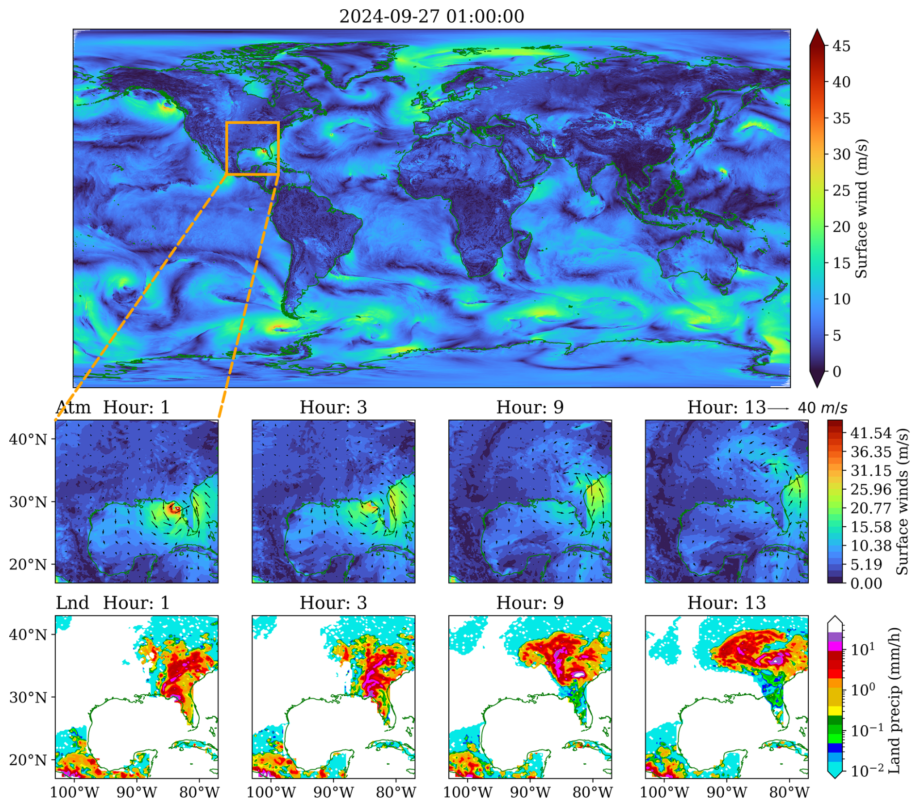
Figure 8 Global surface wind speed (top row) and regional time evolution of atmospheric surface winds (middle row) and precipitation seen by the land component (bottom row) over the southeastern United States and Gulf of America for hours 1, 3, 9 and 13 from 27 September 2024. The orange box indicates the zoomed in region. Black arrows denote the local near-surface wind velocity vectors.

Figure 8 shows surface wind magnitude and vectors from the atmospheric component (middle row) alongside the precipitation field received by the land component (bottom row) at hours 1, 3, 9, and 13 of the simulation. The atmospheric surface winds (middle row) clearly capture the storm's cyclonic circulation, with peak wind speeds exceeding 40 m s⁻¹ concentrated in the eyewall region near the Gulf Coast at hour 1, consistent with major hurricane intensity. The characteristic asymmetric wind structure of a landfalling hurricane is evident, with the right-of-track quadrant exhibiting the strongest winds due to the superposition of the storm's rotational winds and its translational velocity. As the storm progresses through hours 3 to 13, the surface wind field shows progressive weakening over land, reflecting the increased surface roughness and reduced moisture supply that drive the well-known rapid weakening upon landfall. The land precipitation field (bottom row) reveals the spatial coherence between the atmospheric forcing and the land model's received precipitation. The precipitation maximum tracks consistently with the storm's wind circulation center, and the spiral rainband structure visible in both fields confirms that the atmosphere-land coupling is transmitting the storm's mesoscale organization faithfully across the component interface to the land component. The progressive inland penetration of precipitation from hours 1 to 13 demonstrates that the land model receives a physically consistent and temporally continuous forcing through the coupling layer.

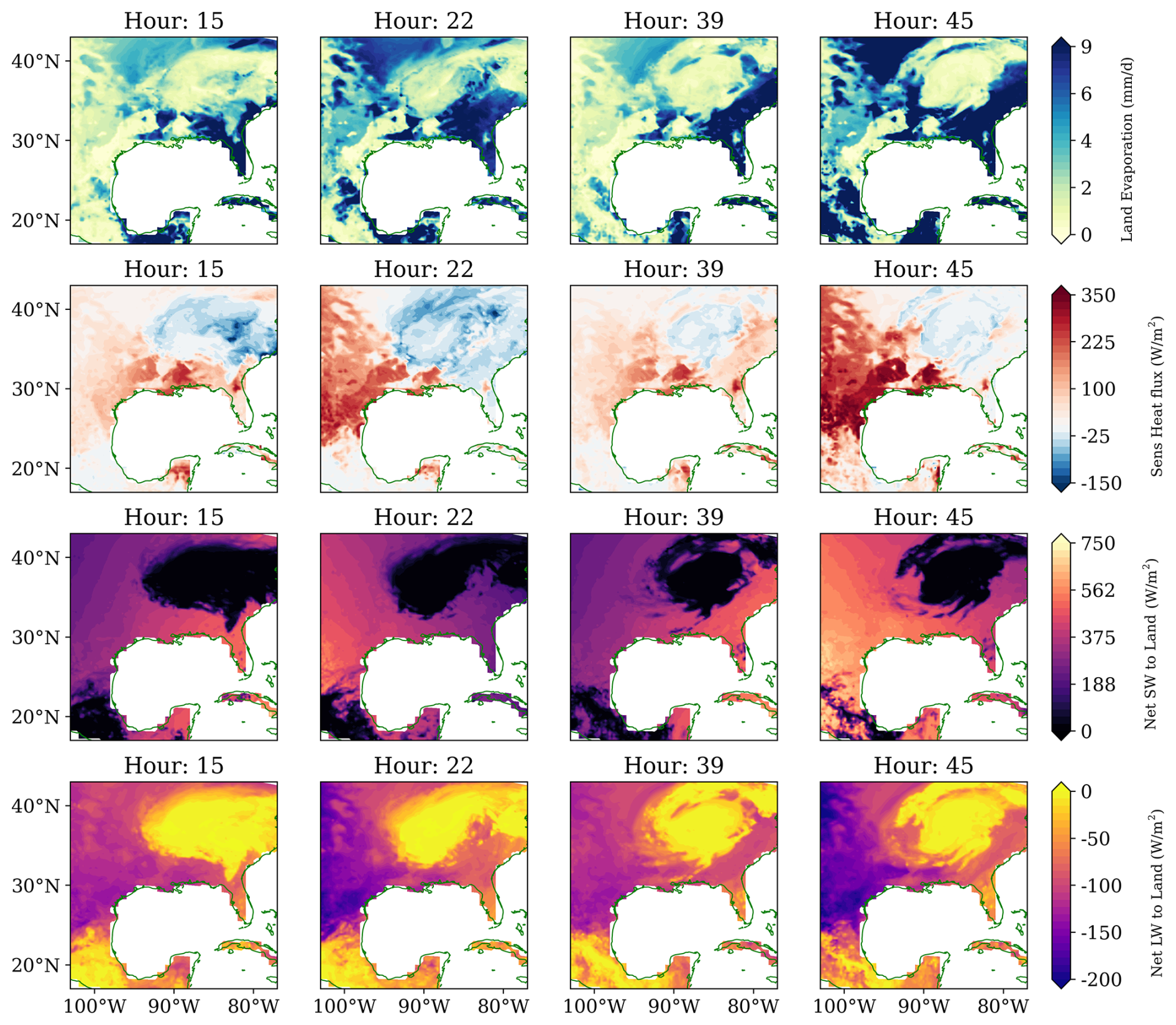
Figure 9 Two-dimensional snapshots of the time evolution of selected diagnostics from the land component: land evaporation (row 1), sensible heat flux (row 2), net shortwave radiation (row 3), and net longwave radiation (row 4) for hours 15, 22, 39 and 45.

Figure 9 shows the evolution of several instantaneous surface fluxes as diagnosed by the land component. The panels depict land evaporation, sensible heat flux, net shortwave radiation and net longwave radiation at hours 15, 22, 39 and 45 and spanning inland throughout the storm progression. Land evaporation displays reduced values beneath persistent heavy rainfall and hurricane clouds and enhanced fluxes once the storm passes. The spatial pattern clearly reflects this competing behavior as expected. The sensible heat flux (row 2) exhibits a pronounced negative anomaly (−150 W m⁻²) collocated with the storm's spiral bands and eye, indicative of suppressed surface shortwave heating and enhanced surface evaporative cooling under the dense cloud shield and heavy precipitation, while positive values exceeding 350 W m⁻² persist in clear-sky regions surrounding the storm. The net shortwave radiation reaching the land surface (row 3) captures a clear diurnal signal modulated by the storm's cloud cover: these plots show values approaching 750 W m⁻² in cloud-free regions, while the storm shadow imposes near-zero shortwave fluxes beneath the cloud canopy, consistent with the optical thickness of hurricane convective systems.

Net longwave radiation exhibits a response complementary to, and opposite of, the net shortwave radiation. Its values are predominantly negative in the clear-sky environment surrounding the storm, where land surface loses longwave radiation freely to the clear atmosphere, while beneath the hurricane's dense clouds the net LW is suppressed toward zero by the downwelling longwave emission from the clouds. The spatial pattern closely follows the cold-core cloud structure, indicating that the model realistically captures the radiative signature of dense clouds. In the outer regions of the storm domain, where cloud cover is warmer and optically thinner, longwave cooling is weaker but remains negative, consistent with a gradual transition from the cloud-free state to the storm's intense core.

Collectively, these diagnostics demonstrate that the land model responds coherently to hurricane forcing, reproducing the expected redistribution of radiative and turbulent energy fluxes across both the storm core and the surrounding environment. The spatial alignment between cloud structure, radiative forcing, and turbulent flux anomalies, as well as their inland displacement with storm progression, indicates dynamically consistent coupling between atmospheric processes and land-surface energetics across the diurnal cycle.

The hydrological response of the land model to Hurricane Helene is examined through complementary diagnostics: soil liquid water content, surface runoff, and river flow with a particular focus on North Carolina, which was severely impacted by the storm's catastrophic flooding.

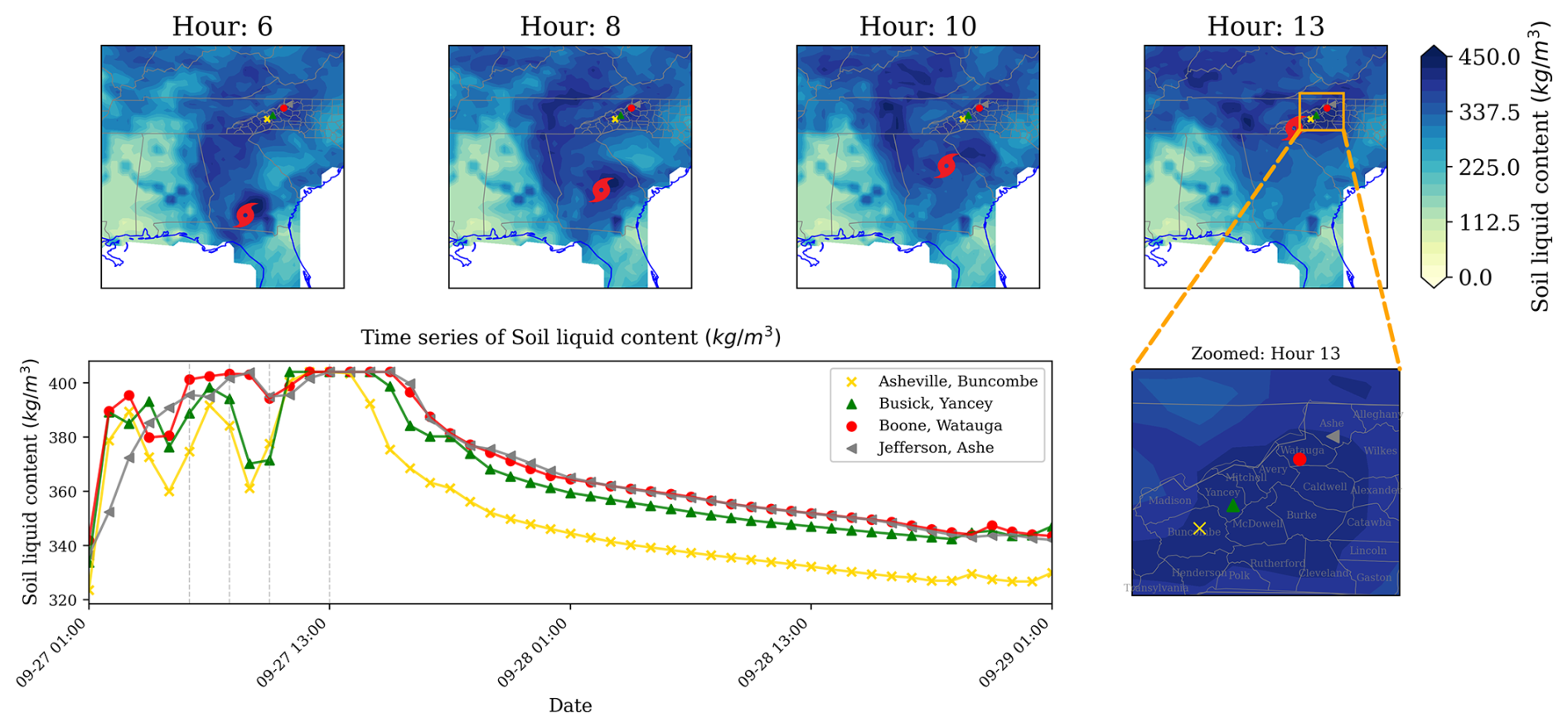
Figure 10 Surface Soil liquid water content of the top soil layer (0.01 m) during Hurricane Helene shown as spatial snapshots at hours 6, 8, 10, and 13 (top), time series at four locations in western North Carolina (bottom left), and a zoomed view of the hour 13 snapshot centered on the western North Carolina region (bottom right). The hurricane symbol indicates the storm's position at each hour. Vertical dashed lines in the time series correspond to the hours shown in the spatial snapshots.

Figure 10 shows the regional spatial distribution of the soil liquid water content in the top soil layer (0.01 m). The spatial map already shows a moderately saturated soil which is the typical condition in late September. As the storm moves inland, the soil becomes highly saturated as shown by the dense blue color of the snapshots. The western North Carolina region shows a progressive increase toward full saturation between hours 6 and 13, with the Asheville area and surrounding counties reaching maximum values exceeding 400 kg m⁻³ by hour 13. In the second row, we consider the time series of soil water content at four different locations, severely hit by the storm: Asheville/Buncombe, Busick/Yancey, Boone/Watauga and Jefferson/Ashe. All four locations reach saturation simultaneously at hour 13 but diverge during the post-storm drainage phase. The Asheville/Buncombe location drains most rapidly, likely reflecting differences in soil texture and topographic slope at that grid cell, while the Boone/Watauga and Jefferson/Ashe locations retain elevated soil moisture for longer, suggesting slower drainage. This spatial heterogeneity in the post-storm recovery is physically realistic and highlights the model's sensitivity to local soil and topographic properties.

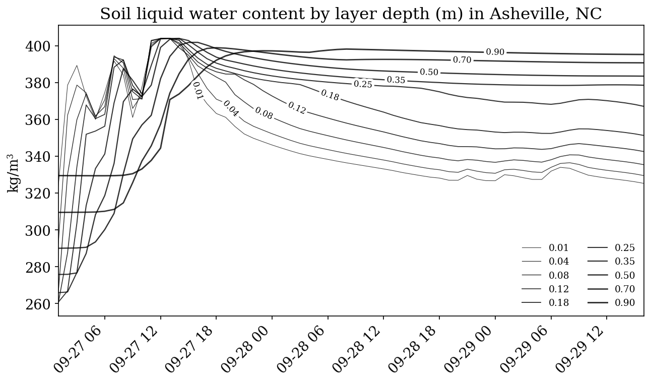
Figure 11 Soil liquid water content (kg m⁻³) at the Asheville/Buncombe grid cell as a function of time during Hurricane Helene, shown for each soil layer depth (m) up to 0.9 m depth.

The point time series at Asheville/Buncombe provides a detailed vertical perspective on the soil saturation process as shown in Fig. 11. Before the storm arrives, soil moisture naturally changes with depth, with different layers showing a typical pattern of variability. As intense storm precipitation reaches the region around 27 September 12:00 Z, all soil layers rapidly converge to saturation at approximately 400 kg m⁻³ in a few hours, demonstrating the land model's ability for water to penetrate downward through the soil column in response to extreme rainfall. Following saturation, the drainage rate is clearly depth-dependent: in shallow layers (0.01–0.12 m) soil water content decreases relatively quickly as gravitational drainage and surface evaporation deplete near-surface moisture, while deeper layers (0.50–0.90 m) remain near saturation for the remainder of the simulation period. This observed behavior is physically consistent.

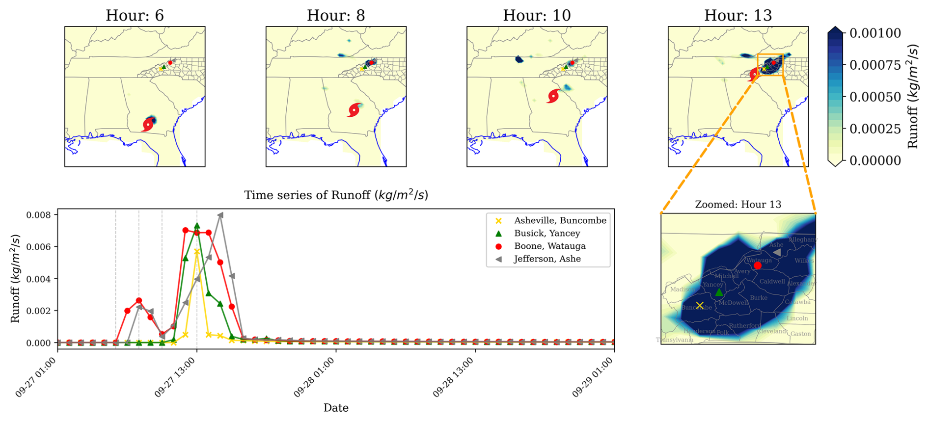
Figure 12 As for Fig. 10 but for land surface runoff.

Once soil approaches saturation, the dominant hydrological process shifts toward runoff. The runoff response is sharp, localized and dramatic, as seen in Fig. 12. Prior to the storm the runoff at all four locations is zero, consistent with unsaturated soil able to absorb incoming precipitation. As the storm's precipitation arrives on 27 September, runoff at Boone/Watauga and Busick/Yancey rises sharply to peak values exceeding 0.006–0.007 kg m⁻² s⁻¹. The peak is extremely brief, lasting a few hours before returning to near-zero values, consistent with the episodic nature of the precipitation forcing. The Jefferson/Ashe location exhibits a slightly delayed and higher runoff peak relative to Boone and Yancey, which may reflect differences in local precipitation intensity or the effect of the already-elevated antecedent soil moisture at that location. The spatial maps confirm that the runoff signal is tightly localized to the southern Appalachians throughout hours 6–13, with the zoomed inset at hour 13 clearly showing the runoff maximum concentrated over the four counties, Buncombe, Yancey, Watauga, Ashe, and surrounding counties. This is precisely the area that experienced catastrophic flash flooding during Hurricane Helene.

The river flow response, shown in Fig. 13, completes the hydrological sequence from precipitation to soil saturation, runoff and ultimately river discharge. All four locations show a rapid increase of 2–3 orders of magnitude in river flow at 27 September 12:00 Z coinciding with the runoff peak but with a discernible lag of several hours that reflects the travel time of water through the river routing network. Jefferson/Ashe exhibits the highest peak river flow, consistent with its position draining a larger area towards larger river routes, while Busick/Yancey shows the lowest peak, likely reflecting a smaller contributing drainage area. Importantly, unlike the runoff signal which decays to near-zero within hours, river flow remains substantially elevated through 30 September, decaying slowly over a multi-day recession characteristic of drainage following extreme flood events. In particular, Asheville/Buncombe and Jefferson/Ashe sustain the highest flow rates during this recession period, consistent with their geographic positions as the primary outlets through which accumulated water exits the flooded mountain region: Asheville draining southward into the Broad River corridor and Jefferson routing flow northeastward into larger downstream networks. This is nicely captured in the snapshots at hours 43 and 56. This multi-day persistence and the spatial differentiation between locations demonstrate that the river routing component is correctly integrating the upstream runoff signal and redistributing it through the drainage network on physically realistic timescales, capturing both the rapid flood onset and the slower drainage that characterized the observed Helene flooding in western North Carolina.

Taken together, these diagnostics describe a physically coherent and complete hydrological response chain: extreme precipitation from Hurricane Helene drives rapid soil saturation at both the regional and local scale, triggering excess runoff generation concentrated in a specific area, which is subsequently routed through the river network producing a multi-day flood. The timing, magnitude, and spatial distribution of each component are consistent with the physical processes expected during a catastrophic landfalling hurricane event, and with the documented impacts of Helene in western North Carolina, providing strong evidence that the land model and its coupling to the atmospheric component are functioning correctly from a qualitative perspective. Further work is underway to quantitatively evaluate the model's performance against observations.

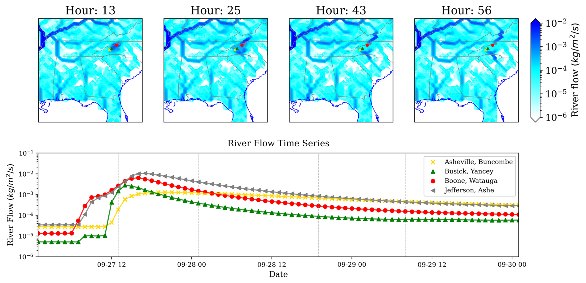
Figure 13 As for Fig. 10 but for river flow for hours 13, 25, 43 and 56.

5 The power of global models

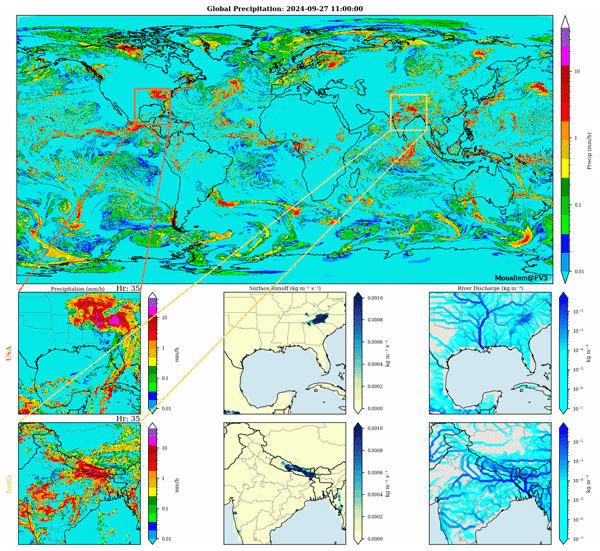
A key advantage of a global coupled atmosphere-ocean-land modeling configuration is its ability to represent multiple, physically independent extreme events occurring simultaneously anywhere on Earth within a single simulation, without any change in model configuration or domain. Figure 14 illustrates this using the same SHiELD-MOM6-LM4 simulation discussed previously. At hour 11 of the simulation, the model simultaneously resolves both Hurricane Helene approaching landfall on the U.S. Gulf Coast and, on the opposite side of the globe, an entirely unrelated and independently forced extreme rainfall event over Nepal and northeastern India that produced some of the most damaging flooding and landslides the region had experienced in decades, with more than 200 fatalities reported and record-breaking rainfall accumulations in the Kathmandu Valley (Lamichhane et al., 2025). In the U.S. sub-domain (middle row), the heaviest precipitation inland is well apparent, consistent with the landfall of Helene. The associated surface runoff is localized in the region of intense rainfall and the river flow exhibits the hydrological response discussed in the previous section. At the same time, over South Asia (bottom row), the model simulates an intense band of rainfall along the Himalayan front. The corresponding surface runoff field shows a well-developed signal centered on the Nepal–India border region, spatially coincident with the districts most severely affected by the September 2024 flooding and landslides events. The river flow panel resolves the dense drainage network of the Ganges–Brahmaputra system and captures the flooding signal.

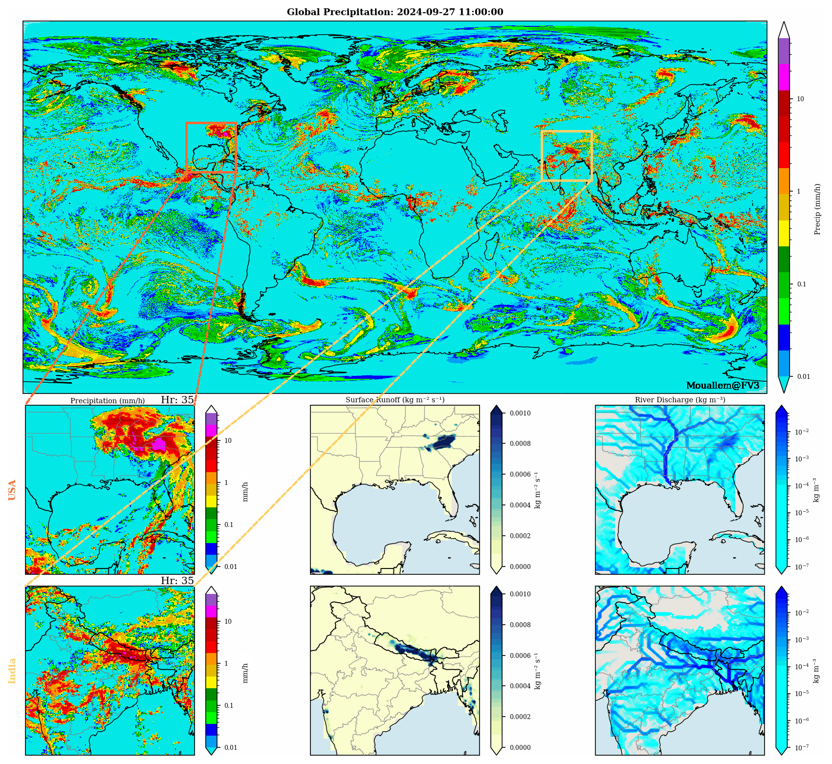
Figure 14 Demonstration of the global model's ability to resolve multiple, independent extreme events within the same simulation. (Top) Global instantaneous precipitation rate; orange boxes mark the two zoomed sub-domains shown below. (Middle row): southeastern US: precipitation, surface runoff and river flow. (Bottom row) As in the middle row but for the South Asia domain including Nepal, India, Bangladesh

This single snapshot demonstrates that a single global simulation of the coupled SHiELD–MOM6–LM4 system can simultaneously represent the atmospheric forcing and land-surface hydrological response associated with two simultaneous, geographically unrelated extreme events. This capability highlights the value of global coupled modeling systems for multi-hazard monitoring and early warning, where forecasters and disaster-management agencies must anticipate concurrent extreme events occurring in different regions of the world within the same forecast cycle.

6 Conclusions

We have successfully integrated GFDL's land model LM4 into SHiELD. Using the FMS coupler infrastructure, the atmospheric code and drivers were refactored to enable implicit land model coupling while maintaining modularity and flexibility. This implementation transforms SHiELD into a fully coupled Earth system model, employing MOM6/SIS2 for the ocean–sea ice system and LM4 for land and hydrological processes. Importantly, the component integration preserves the ability to run the original ocean and land physics suites within the same runtime environment, using one source code and executable, ensuring backward compatibility and facilitating controlled experimentation.

The inclusion of LM4 significantly enhances the representation of land–atmosphere interactions, enabling physically consistent treatment of hydrological processes, cryospheric dynamics, soil moisture evolution, river routing, vegetation processes, and disturbance-driven aerosol emissions (such as those arising from wildfires), and other available capabilities not shown here. These capabilities are essential for realistically simulating extreme hydroclimate events and compound hazards across weather to climate timescales.

We demonstrated the new configuration using the landfall of Hurricane Helene of 2024 as a case study, highlighting the land response to extreme precipitation and strong surface forcing. The evolution of soil moisture, runoff, and river discharge exhibited physically consistent behavior and qualitatively validated the technical coupling strategy. The land surface responded dynamically to storm-driven forcing, providing confidence in the integrity of the flux exchanges and state updates across model components. Ongoing work focuses on systematic evaluation of the fully coupled SHiELD forecast skill across multiple timescales, from short-range weather prediction to subseasonal-to-seasonal (S2S) applications. Assessments include precipitation, surface fluxes, soil moisture memory, land–atmosphere feedback strength, sensitivity to land initialization, coupling frequency, and resolution, as well as the role of interactive land processes in improving forecasts at high resolution. Stability for longer lead times has also been assessed; a simulation with a coarser atmosphere resolution has integrated stably for over a year and maintained a stable climate with minimal drift, demonstrating the utility for subseasonal and longer coupled Earth-system integrations.

The fully coupled SHiELD model represents a major step toward a seamless, high-resolution Earth system modeling framework. By unifying atmosphere, ocean, sea ice, and land components within a consistent infrastructure, this development lays the foundation for improved prediction of extreme events, enhanced understanding of cross-component feedbacks, and a more integrated approach to weather–climate research.