A novel Gauss-Hermite High-Order Sampling Hybrid ensemble filter for computationally efficient data assimilation in geosciences – Part 1: Application to Lorenz-96 in PythonDA v1.2.2

Data assimilation is used in a number of geophysical applications to optimally integrate information from observations and models. Providing an estimation of both state and uncertainty, ensemble algorithms are among the most successful data assimilation approaches. Since the estimation quality depends on the ensemble, the sampling method is a crucial step in ensemble data assimilation. This work introduces a sampling method featuring a higher polynomial order of approximation, and an ensemble filter, the Gauss-Hermite High-Order Sampling Hybrid filter (GHOSH), which exploits the higher order of the novel sampling method. In contrast, the order of the most frequently adopted ensemble algorithms in geosciences is usually equal to or lower than 2. In the directions where the uncertainty is larger, the GHOSH filter's sampling method achieves a higher order of approximation than in other ensemble-based filters, without increasing the asymptotic computational complexity that is comparable to that of second-order deterministic filters. To evaluate the benefits of the higher approximation order, a set of twin experiments of Lorenz96 simulations has been carried out using the GHOSH filter and a second-order ensemble Kalman filter (SEIK; singular evolutive interpolated Kalman filter). The twin-experiment results show that GHOSH outperforms SEIK in most of the assimilation settings, with up to a 56 % reduction of the root mean square error on assimilated and non-assimilated variables when best-tuned forgetting factors are adopted for each filter.

1 Introduction

Data assimilation (DA) methodologies provide a conceptual framework to integrate the information content embedded in observations and numerical models, and play a pivotal role in deriving accurate estimates of the state of Earth systems components and reducing the uncertainties of geophysical systems (among others, see the methods and applications reviewed in Carrassi et al., 2018; Houtekamer and Zhang, 2016; Lahoz and Schneider, 2014; van Leeuwen et al., 2019; Martin et al., 2015; Roth et al., 2017; Vetra-Carvalho et al., 2018).

Thanks to the scalability of parallel implementations, the use of ensemble algorithms (see e.g., Vetra-Carvalho et al., 2018; Houtekamer and Zhang, 2016; Bannister, 2017, and references therein) has been proposed to estimate uncertainty and improve assimilation skills in Kalman filters and variational methodologies. On the other hand, some of the strong points of ensemble and variational methods have been merged in hybrid filters (e.g., Hamill and Snyder, 2000). Moreover, recent developments of EnKF have been conceived to face increasing nonlinearities and model complexity that are also related to the expanding availability of observations and computational resources (as discussed in, e.g., Vetra-Carvalho et al., 2018).

However, the definition of the strategy for ensemble generation is not a trivial task (see e.g., Moore et al., 2019). Straightforward Monte Carlo approaches are not usually a viable option in geoscience applications, because they would require too large a number of ensemble members, and consequently, computational effort. The number of ensemble members can be reduced by adopting deterministic sampling methods (as opposed to stochastic EnKF methods, see e.g. Carrassi et al., 2018; Houtekamer and Zhang, 2016; Nerger et al., 2005; Lahoz and Schneider, 2014, and the references therein).

Common examples of deterministic EnKF are SEIK (Pham, 2001) and ETKF (Bishop et al., 2001). According to Pham (2001), these are second-order exact methods, where the term order refers to polynomial exactness (in contrast with the order convergence in ensemble size in Monte Carlo stochastic methods or the time-integration order in numerical methods). We want to extend this concept by introducing here the notion of polynomial order of approximation of the filter or of its sampling method or, more concisely, order: a hth-order ensemble has the property of providing a forecast mean with no error if a hth-order polynomial model is used for forecasting. According to this definition, SEIK and ETKF are second-order methods, while Monte Carlo sampling has order zero. As proven in Appendix A, hth-order is achieved by sampling an ensemble that matches the first h statistical moments of the uncertainty probability density function (pdf) before evolution (also called prior in Bayesian statistics).

Most of the models used in geoscience applications are based on systems of differential equations that cannot be represented by a second-order polynomial and in all of these cases the second-order sampling methods provide a non-exact estimation of the forecast mean, which is affected by an error strictly related to the approximation error that would be made if approximating the model by a second-order polynomial. Furthermore, the second-order approximation of the forecast mean is more effective the closer the ensemble members are to each other (i.e., small uncertainty), thus the higher the uncertainty the worse will be the approximation error in the mean computation. Since the state estimation is often affected by a relatively high uncertainty in geosciences data assimilation applications, this approximation error may not be negligible.

A potential strategy to reduce this error is the use of a higher order of approximation. In general, this would require a larger ensemble with respect to the second-order methods and consequently larger computational costs. Indeed, a higher order of approximation implies a larger number of ensemble members to represent the same uncertainty subspace¹. For instance, second-order methods use an ensemble of r+1 members to span an r-dimensional uncertainty subspace (e.g., Pham, 2001), while 2r ensemble members (see Appendix C4) are needed to achieve order 3 in the same subspace (see e.g., Wan and Van Der Merwe, 2000; Ambadan and Tang, 2009; Luo and Moroz, 2009, for examples of third-order method with 2r+1 ensemble members).

Weighted ensembles can achieve higher order while mitigating the ensemble size increase with respect to non-weighted ensembles. In the literature, based on the multi-dimensional Gauss-Hermite quadrature rule (Mastroianni and Milovanovic, 2008, chap. 2), the use of a weighted ensemble has been applied to achieve a higher order of approximation but still at the cost of a larger ensemble size (Ito and Xiong, 2000) with respect to second-order methods. It is worth noting that weighted ensembles are also exploited in particle filter methods (van Leeuwen et al., 2019), where weights are used to evolve both the ensemble members and their probability.

In the present work, we propose a novel weighted ensemble method based on a new high-order sampling that identifies subspaces of larger uncertainties and provides ensemble mean estimates of order higher than 2 in those specific subspaces, without increasing the overall number of ensemble members, and therefore without major impacts on the computational cost. In this sense, our approach presents the same computational complexity and number of ensemble members as existing deterministic ensemble approaches (e.g., SEIK or ETKF) but exploits the advantage of a higher order only where the approximation errors are larger.

The proposed high-order filter (as does its sampling method) exploits a Gauss-Hermite-like quadrature rule, along with a principal component analysis (PCA), and we named it Gauss-Hermite high-order sampling hybrid (GHOSH) filter. Members and related weights are chosen in such a way as to guarantee accuracy of order higher than 2 for a subset of principal modes, and no less than 2 for the remaining ones. The GHOSH filter exploits a hybrid approach that considers the uncertainty as composed of a constant and a time-evolving ensemble-based part.

The reliability of the new filter is demonstrated in a large set of twin experiments based on an idealized model commonly used to test DA methodologies (Lorenz, 1996). In a companion paper (Spada et al., 2026) the new filter is tested in the much more complex and realistic marine biogeochemical application currently used in the Copernicus Marine (CMEMS) system (Salon et al., 2019), featuring assimilation of satellite observations (Spada, 2024).

Section 2 introduces the novel elements of the high-order sampling and Sect. 3 presents a synthetic description of the GHOSH algorithm and its localized version. The Lorenz96 numerical experiment is introduced in Sect. 4 and its results are presented in Sect. 5. The algorithm and the experimental results are discussed in Sect. 6. Finally, additional mathematical and algorithmic details along with examples are provided in appendices.

2 The high-order sampling

In this work we propose a novel method to generate ensembles for data assimilation applications. The preliminary idea is that the more statistical moments are shared by an uncertainty pdf and an ensemble representing it, the lower the error made by the ensemble in the forecast mean (Appendix A). In this sense, an ensemble of order h, that is characterized by the property of matching the uncertainty pdf up to the moment of order h, provides a more accurate forecast mean than an ensemble of order lower than h. Compared to deterministic second-order square-root sampling methods, whose ensembles match the first 2 statistical moments of the uncertainty pdf, the novel strategy achieves an ensemble with a higher order of approximation (i.e., matching more than 2 statistical moments) without increasing the ensemble size. The strategy is based on the choice, among all the second-order ensembles, of those that feature a higher order of approximation along the principal components of the uncertainty (i.e., those directions where the ensemble spread is larger and the approximation is consequently worse).

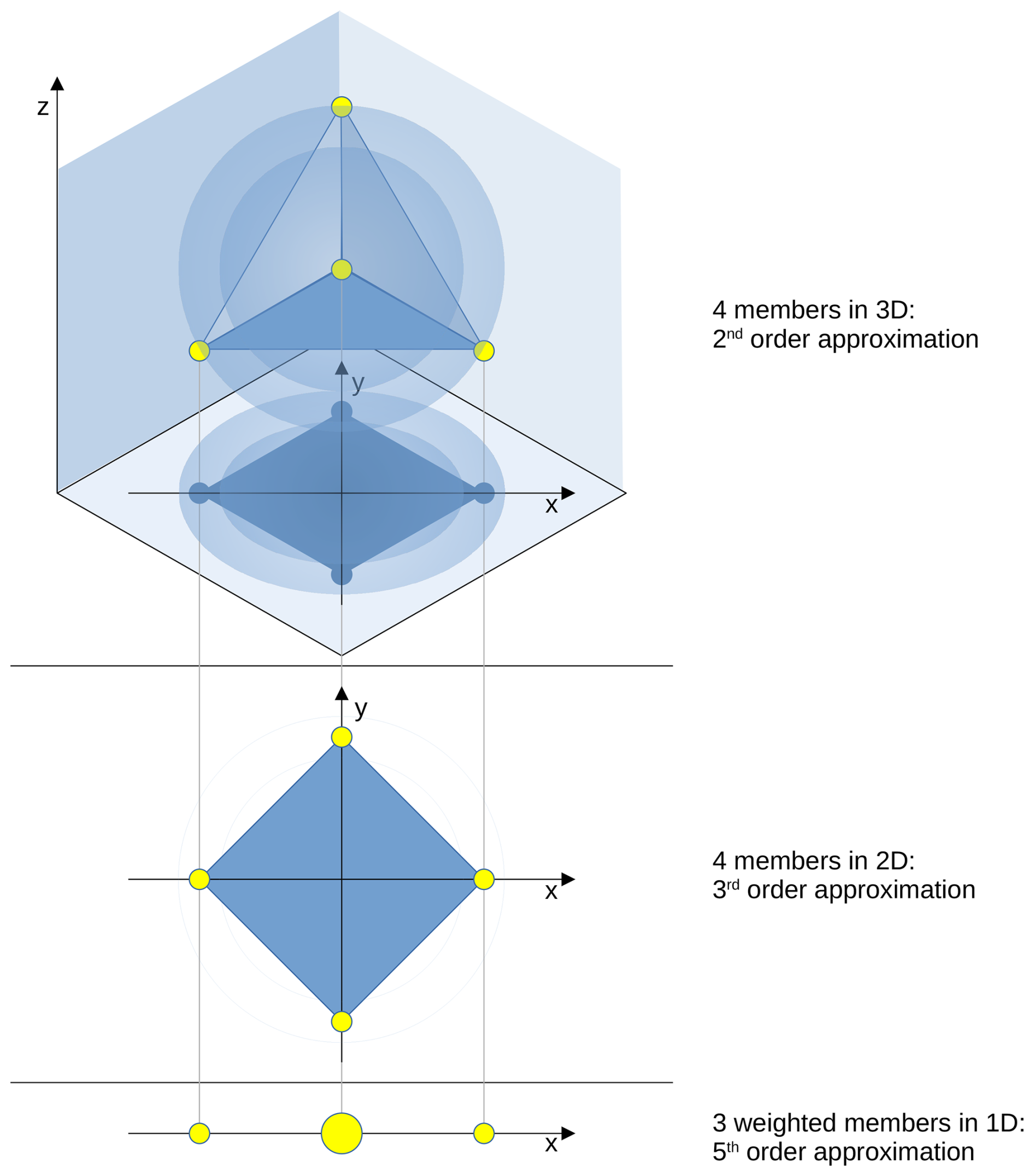
Figure 1 Four tetrahedron-shaped ensemble members (yellow dots) in a 3-dimensional space (top) represent a second-order approximation of a standard normal distribution (with the spherical isosurfaces shown in shadow). The same four members form a square in two dimensions (middle), producing a third-order approximation. By projecting further into one dimension (bottom) and by assigning proper weights, a fifth-order approximation is obtained.

Figure 1 shows an uncertainty represented by a 3-dimensional standard normal distribution in an xyz Cartesian coordinate system (top of Fig. 1 where spherical uncertainty isosurfaces are represented by shadowed areas). According to the second-order-exact sampling (Pham, 2001), four opportunely chosen ensemble members are needed to represent this uncertainty probability density function up to the second order. The ensemble members are not uniquely determined by the second-order exact sampling, which indeed allows for random rotations. In the xyz Cartesian coordinate system of Fig. 1, four ensemble members that ensure the second-order exact sampling (yellow points at the vertices of a regular tetrahedron) are chosen among all the possible second-order sampling (each corresponding to a rotation of the tetrahedron). Thanks to their particular orientation, the four vertices draw (project) a square (a non-skewed shape) in the xy plane (middle panel of Fig. 1; Appendix C3.1), achieving a third-order approximation in the xy plane. Indeed, four square-shaped ensemble members provide a third-order approximation for a 2-dimensional normal distribution (Appendix C2.4). Similarly, there are other possible choices of second-order vertices that project a square (third-order approximation) in the xy plane, but thanks to this particular orientation, the four members chosen in Fig. 1 can be further projected along the x-axis to obtain the special 3-point distribution (shown at the bottom of Fig. 1), where the central projected point weights as two of the original points. As it is, this 1-dimensional distribution does not achieve an order higher than 3 (already achieved in the xy plane with the square projection) along the x axis but three properly weighted ensemble members can reach an approximation order as high as 5 on the x axis (not shown in Fig. 1, see Appendix C1.3). On the contrary, if proper weights are not assigned, the highest approximation order that can be obtained using 4 members in the 1-dimensional case is limited to 3. In summary, Fig. 1 represents an example of an ensemble with approximation order 2 in the xyz 3-dimensional space, which is opportunely oriented to have approximation order 3 in the xy plane and, by assigning proper weights, can reach approximation order 5 along the x axis (Appendix C3.2). Generally, the possibility to increase the approximation order using appropriate rotations and weights opens the way to build an ensemble with a higher order of approximation along dimensions where uncertainties are higher. For instance, in the case of a non-standard normal distribution (in contrast with the 3-dimensional standard distribution of Fig. 1), if the orientation of the xyz coordinate system was chosen so that the z component of the distribution was less relevant than the x and y components, then the ensemble built with the third-order approximation would mitigate the approximation error in the x and y dimensions where the spread is higher. Similarly, if the coordinate system is oriented so that the variance is larger on x than y, then the achieved fifth-order approximation reduces the error more efficiently where the spread is maximum (x coordinate). As shown later in this work, the high-order sampling mimics this strategy in the ensemble data assimilation context, in order to achieve a higher order in the uncertainty principal components.

The high-order sampling generalizes the idea described above considering that any probability distribution (under reasonable hypothesis) can be sampled with high order of approximation with a weighted ensemble that, in the special case of the Gaussian distribution, is represented by the nodes and weights of the Gauss-Hermite quadrature rule (Mastroianni and Milovanovic, 2008, chap. 2). Once the approximation order (h larger than 2) and the ensemble size (r+1) are fixed, the hth-order weighted ensemble is computed for a relatively small s-dimensional subspace (s lower than r); then, a new (r+1)-sized second-order weighted ensemble is computed such that its projections along the uncertainty principal components coincide with the hth-order ensemble. The resulting ensemble has a second-order approximation in the r-dimensional subspace and a hth-order approximation in the s-dimensional subspace of the principal uncertainty directions. By comparison, a second-order-exact sampling (e.g., SEIK) with r+1 ensemble members would provide a second-order approximation for the whole r-dimensional subspace.

It is worth noting that this approach is beneficial independently of the uncertainty pdf. Even in the Gaussian case, where the uncertainty pdf is uniquely determined by its mean and covariance, the ensemble is not uniquely determined in the same way. Thus, building an ensemble matching also higher Gaussian moments helps to better represent the uncertainty pdf, which in turn translates in a smaller error on the forecast mean.

The two phases of the high-order sampling (initialization and sampling) are described in the following from an algorithmic point of view. The initialization includes the steps that must be executed only once, while the sampling presents the ensemble generation procedure. In the sampling description, the system of equations to compute the ensemble perturbations and weights is presented. As the ensemble moments are used in the sampling phase but are calculated only once, their calculation is presented in the initialization section. Mathematical explanations can be found in Appendix A.

2.1 Initialization

2.1.1 Initialization of the hyper-parameters

In the high-order sampling, two sets of hyper-parameters need to be defined.

The first set includes: the higher approximation order h reached in the principal components of the uncertainty subspace; the dimension of the uncertainty subspace r, which implies an ensemble size of r+1 members; and s, that represents the number of principal components that are approximated with the higher order h and that must be smaller than r.

The second set includes the parameterized statistical moments of the typical uncertainty, i.e. the centered moments up to order h of an uncorrelated and normalized pdf in the subspace of dimension s. The statistical moments of the normalized pdf are preliminary to the sampling algorithm, which takes mean and covariance as input and rescales all the moments accordingly (see later Eq. 6).

Noted as ${\mathit{\mu }}_{j_{\mathrm{1}},\mathrm{\dots },j_{\mathit{\xi }}}$, a generic moment of order ξ has ξ indices, each of which runs between 1 and s. A common choice for the parameterized pdf comes from the standard normal distribution 𝒩(0,I_s), which leads to moments

$$\begin{array}{}\text{(1)}& {\mathit{\mu }}_{j_{\mathrm{1}},\mathrm{\dots },j_{\mathit{\xi }}}=\underset{{\mathbb{R}}^s}{\int }{z}_{j_{\mathrm{1}}}\mathrm{\cdots }{z}_{j_{\mathit{\xi }}}\mathit{\phi }\left(\mathit{z}\right)d\mathit{z},\end{array}$$

where φ is the pdf corresponding to 𝒩(0,I_s). In the Gaussian case, the moments ${\mathit{\mu }}_{j_{\mathrm{1}},\mathrm{\dots },j_{\mathit{\xi }}}$ can easily be computed (i.e., without solving numerically the integral, see Appendix A, Eq. A6). Instead, other non-Gaussian probability distributions can be explored considering their specific moments ${\mathit{\mu }}_{j_{\mathrm{1}},\mathrm{\dots },j_{\mathit{\xi }}}$.

However, since the parameterized pdf is uncorrelated and normalized, only centered moments of order higher than 2 are actual hyper-parameters (i.e., ${\mathit{\mu }}_{j_{\mathrm{1}},\mathrm{\dots },j_{\mathit{\xi }}}$ with ξ>2), while moments up to order 2 are always already defined.

2.1.2 Initialization of the ensemble weights and of the sampling matrix

In the initialization phase, the ensemble weights and the sampling matrix Ω^h are computed by imposing the matching between the statistical moments up to order h of the ensemble and the parameterized uncertainty pdf (Eq. 2). The ensemble weights and the sampling matrix are constant elements that must be prepared only once for a given set of hyper-parameters.

The real numbers u_m,j and v_m, with $j\in \left\{\mathrm{1},\mathrm{\dots },s\right\}$ and $m\in \left\{\mathrm{1},\mathrm{\dots },r+\mathrm{1}\right\}$, represent the entries of Ω^h and the square roots of the ensemble weights respectively. The ensemble matrix is built such that the numbers $u_{m,j}/v_m$ represent the ensemble anomalies in a s-dimensional space (see Appendix A), thus they are calculated as a solution of the nonlinear system

$$\begin{array}{}\text{(2)}& \left\{\begin{array}{l}\mathrm{⋮}\\ {\displaystyle }\sum _{m=\mathrm{1}}^{r+\mathrm{1}}{u}_{m,j_{\mathrm{1}}}\mathrm{\cdots }{u}_{m,j_{\mathit{\xi }}}{v_m}^{\mathrm{2}-\mathit{\xi }}={\mathit{\mu }}_{j_{\mathrm{1}},\mathrm{\dots },j_{\mathit{\xi }}}\\ \mathrm{⋮}\end{array}\right.\end{array}$$

with one equation for each $\mathit{\xi }\in \left\{\mathrm{0},\mathrm{\dots },h\right\}$ and for each $j_{\mathrm{1}},\mathrm{\dots },j_{\mathit{\xi }}\in \left\{\mathrm{1},\mathrm{\dots },s\right\}$, for a total of $\left(s^{h+\mathrm{1}}-\mathrm{1}\right)/\left(s-\mathrm{1}\right)$ equations. The system represents the matching between the statistical moments up to order h of the ensemble and the parameterized uncertainty pdf (this condition is necessary to achieve hth-order, as proven in Appendix A). In fact, the equation of system (2) for ξ=0, i.e.,

$${\displaystyle }\sum _{m=\mathrm{1}}^{r+\mathrm{1}}{v_m}^{\mathrm{2}}=\mathit{\mu }=\mathrm{1},$$

ensures that the weights will sum to 1; the s equations for ξ=1, i.e.,

$$\left\{\begin{array}{l}{\displaystyle }\sum _{m=\mathrm{1}}^{r+\mathrm{1}}{u}_{m,\mathrm{1}}{v}_m={\mathit{\mu }}_{\mathrm{1}}=\mathrm{0}\\ \mathrm{⋮}\\ {\displaystyle }\sum _{m=\mathrm{1}}^{r+\mathrm{1}}{u}_{m,s}{v}_m={\mathit{\mu }}_s=\mathrm{0},\end{array}\right.$$

ensure that the anomalies have 0-mean; the s² equations for ξ=2, i.e.,

$$\left\{\begin{array}{l}{\displaystyle }\sum _{m=\mathrm{1}}^{r+\mathrm{1}}{u}_{m,\mathrm{1}}{u}_{m,\mathrm{1}}={\mathit{\mu }}_{\mathrm{1},\mathrm{1}}={\mathit{\delta }}_{\mathrm{1},\mathrm{1}}=\mathrm{1}\\ \mathrm{⋮}\\ {\displaystyle }\sum _{m=\mathrm{1}}^{r+\mathrm{1}}{u}_{m,\mathrm{1}}{u}_{m,s}={\mathit{\mu }}_{\mathrm{1},s}={\mathit{\delta }}_{\mathrm{1},s}=\mathrm{0}\\ \\ \mathrm{⋮}\\ \\ {\displaystyle }\sum _{m=\mathrm{1}}^{r+\mathrm{1}}{u}_{m,s}{u}_{m,\mathrm{1}}={\mathit{\mu }}_{s,\mathrm{1}}={\mathit{\delta }}_{s,\mathrm{1}}=\mathrm{0}\\ \mathrm{⋮}\\ {\displaystyle }\sum _{m=\mathrm{1}}^{r+\mathrm{1}}{u}_{m,s}{u}_{m,s}={\mathit{\mu }}_{s,s}={\mathit{\delta }}_{s,s}=\mathrm{1},\end{array}\right.$$

force the ensemble covariance matrix to be equal to the identity matrix; and the same holds for higher moments up to h ($\mathrm{2}<\mathit{\xi }\le h$). The general equation reported in system (2) represents all the moment-matching equations up to order h, where ${\mathit{\mu }}_{j_{\mathrm{1}},\mathrm{\dots },j_{\mathit{\xi }}}$ are the prescribed statistical moments of a s-dimensional probability distribution that approximates the assumed uncertainty distribution shape.

The system solution is used to define Ω^h, as the $\left(r+\mathrm{1}\right)\times s$ matrix with entries u_m,j, and the ensemble weight vector $\mathit{w}\in {\mathbb{R}}^{\left(r+\mathrm{1}\right)}$, as the element-wise square of v, i.e.,

$$\begin{array}{}\text{(3)}& \mathit{w}=\left({v_{\mathrm{1}}}^{\mathrm{2}},\mathrm{\dots },{v_{r+\mathrm{1}}}^{\mathrm{2}}\right).\end{array}$$

Note that, in order to actually have at least one solution of the system, the number of independent equations cannot be larger than the number of variables, which implies that given r (and consequently the ensemble size) a larger approximation order h implies a smaller s (i.e., a smaller number of components approximated with order h).

2.2 Sampling

Unlike non-varying quantities (as those defined in the initialization phase), i-indexed quantities appearing in this section are specific of each sampling.

Given an N-dimensional state space, in the sampling phase a new ensemble is generated based on the ensemble mean x_i∈ℝ^N and the covariance matrix ${\mathbf{L}}_i{\mathbf{L}}_i^T$. Since an explicit covariance matrix might be intractable for large N, the N×r matrix L_i is adopted as an r-rank factorization of the covariance matrix and its columns represent the basis of the uncertainty subspace spanned by the ensemble members.
The key idea of this section is to project the high-order ensemble encoded in the sampling matrix Ω^h onto the principal components of the uncertainty subspace, identified by an eigenvalue decomposition.

In order to avoid inducing a bias in the available unexploited degrees of freedom of the sampling, the matrix Ω_i is built from Ω^h by a procedure that includes random symmetries and rotations. These random transformations explore only degrees of freedom that do not compromise the high-order approximation on the principal components of the uncertainty subspace. To achieve this, a random s×s orthogonal matrix ${\mathbf{\Omega }}_i^{\mathrm{rnd}}$ is drawn, then the $\left(r+\mathrm{1}\right)\times \left(s+\mathrm{1}\right)$ matrix $\left(\mathit{v}|{\mathbf{\Omega }}^h{\mathbf{\Omega }}_i^{\mathrm{rnd}}\right)$ is completed to an $\left(r+\mathrm{1}\right)\times \left(r+\mathrm{1}\right)$ orthogonal matrix by the $\left(r+\mathrm{1}\right)\times \left(r-s\right)$ matrix ${\mathbf{\Omega }}_i^{⟂}$, i.e.,

$$\begin{array}{}\text{(4)}& \begin{array}{rl}& (\begin{array}{ccccc}\mathit{v}& |& {\mathbf{\Omega }}^h{\mathbf{\Omega }}_i^{\mathrm{rnd}}& |& {\mathbf{\Omega }}_i^{⟂}\end{array}{)}^T\cdot \\ & \cdot \left(\begin{array}{ccccc}\mathit{v}& |& {\mathbf{\Omega }}^h{\mathbf{\Omega }}_i^{\mathrm{rnd}}& |& {\mathbf{\Omega }}_i^{⟂}\end{array}\right)={\mathbf{I}}_{r+\mathrm{1}},\end{array}\end{array}$$

where v is the array of the square roots of the weights (as in Eq. 3) and I_r+1 is the identity matrix of rank r+1. A procedure for randomly building or completing orthogonal matrices is described in Appendix B.

Now, the $\left(r+\mathrm{1}\right)\times r$ matrix Ω_i, defined as

$$\begin{array}{}\text{(5)}& {\mathbf{\Omega }}_i=\left(\begin{array}{ccc}{\mathbf{\Omega }}^h{\mathbf{\Omega }}_i^{\mathrm{rnd}}& |& {\mathbf{\Omega }}_i^{⟂}\end{array}\right),\end{array}$$

can be used to build the $N\times \left(r+\mathrm{1}\right)$ ensemble matrix X_i:

$$\begin{array}{}\text{(6)}& {\mathbf{X}}_i={\mathit{x}}_i{\mathbb{1}}_{\mathrm{1}\times \left(r+\mathrm{1}\right)}+{\mathbf{L}}_i{{\mathbf{C}}_i}^T{{\mathbf{\Omega }}_i}^T{\mathbf{W}}^{-\frac{\mathrm{1}}{\mathrm{2}}},\end{array}$$

where 𝟙 is a matrix (of the subscripted size) filled with ones, W=diag(w) is the $\left(r+\mathrm{1}\right)\times \left(r+\mathrm{1}\right)$ diagonal matrix of weights and C_i is a r×r orthogonal change-of-basis matrix such that

$$\begin{array}{}\text{(7)}& {{\mathbf{L}}_i}^T{{\mathbf{\Lambda }}_i}^{-\mathrm{1}}{\mathbf{L}}_i={\mathbf{C}}_i^T{\mathbf{E}}_i{\mathbf{C}}_i.\end{array}$$

In the last equation, the right-hand side is an eigenvalue decomposition of the left-hand side, with E_i being an r×r diagonal matrix of eigenvalues in descending order and Λ_i being an appropriate N×N matrix. The purpose of Λ_i is to weight the product between L_i and its transpose; therefore, Λ_i defines the criterion that decides the relative importance of different parts of the state vector, affecting the uncertainty principal components. In relatively simple applications, Λ_i can be the identity matrix, but in most scenarios, Λ_i needs to be properly designed. For example, if different variables represent non-comparable quantities, it is common to standardize such variables by dividing by their standard deviation before computing the PCA. In the formalism of Eq. (7), this is equivalent to defining Λ_i as the diagonal matrix of the uncertainty variance (i.e., the square norm of the rows of L_i). Further discussion on Λ_i can be found in Sect. 6 and Part 2 (Spada et al., 2026).

The orthogonal matrix C_i is fundamental for orienting the ensemble in such a way that the uncertainty principal components align with the directions achieving the higher approximation order (which are encoded in the Ω_i matrix). After computing X_i, the ensemble members can be retrieved from the columns of the matrix, i.e.,

$$\begin{array}{}\text{(8)}& {\mathbf{X}}_i=\left({\mathit{x}}_i^{\mathrm{1}},\mathrm{\dots },{\mathit{x}}_i^{\left(r+\mathrm{1}\right)}\right).\end{array}$$

3 The GHOSH filter

Similar to other data assimilation ensemble schemes, the GHOSH filter provides an estimate of the state of a system at some discrete times t_i in terms of the state vector and the covariance matrix representing the estimation uncertainty. Hence, at time t_i, a forecast is composed of the forecast state vector ${\mathit{x}}_i^{\mathrm{f}}\in {\mathbb{R}}^N$ (N is the dimension of the state space) and the forecast uncertainty covariance matrix ${\mathbf{P}}_i^{\mathrm{f}}$. If an observation vector y_i is available at time t_i, the information is assimilated in the analysis state vector ${\mathit{x}}_i^{\mathrm{a}}$ with uncertainty covariance matrix ${\mathbf{P}}_i^{\mathrm{a}}$.

Being an ensemble-based filter scheme, the GHOSH filter represents these quantities by an ensemble of state vectors, e.g.,

$$\begin{array}{}\text{(9)}& {\mathbf{X}}_i^{\mathrm{f}}=\left({\mathit{x}}_i^{\mathrm{f},\mathrm{1}},\mathrm{\dots },{\mathit{x}}_i^{\mathrm{f},\left(r+\mathrm{1}\right)}\right)\end{array}$$

of r+1 model state realizations. However, unlike other ensemble filters that uniformly weight the ensemble members, the GHOSH filter assigns to ${\mathbf{X}}_i^{\mathrm{f}}$ a vector of corresponding weights

$$\begin{array}{}\text{(10)}& \mathit{w}=\left(\begin{array}{c}{w}_{\mathrm{1}}\\ \mathrm{⋮}\\ w_{r+\mathrm{1}}\end{array}\right).\end{array}$$

The state estimate is given by the weighted mean

$$\begin{array}{}\text{(11)}& {\mathit{x}}_i^{\mathrm{f}}=\sum _{j=\mathrm{1}}^{r+\mathrm{1}}{\mathit{x}}_i^{\mathrm{f},j}{w}_j={\mathbf{X}}_i^{\mathrm{f}}\mathit{w},\end{array}$$

while the uncertainty covariance is approximated by the ensemble covariance matrix

$$\begin{array}{}\text{(12)}& {\mathbf{P}}_i^{\mathrm{f}}\approx {\mathbf{X}}_i^{\mathrm{f}}\mathbf{W}{{\mathbf{X}}_i^{\mathrm{f}}}^T-{\mathit{x}}_i^{\mathrm{f}}{{\mathit{x}}_i^{\mathrm{f}}}^T,\end{array}$$

with W=diag(w) being the diagonal matrix of weights. As in other ensemble-based filter schemes, the uncertainty covariance never needs to be explicitly computed. However, Eq. (12) and the like (e.g., Eqs. 19, 22, 31, 33) are still shown in this form for convenience.

The GHOSH algorithm consists of 5 phases, i.e., initialization, forecast, forecast high-order sampling, analysis and analysis high-order sampling (Fig. 2). The initialization is performed once at the beginning of the filter application, the forecast and forecast high-order sampling phases are carried out at each time t_i, and analysis and analysis high-order sampling are executed only when observations are available.

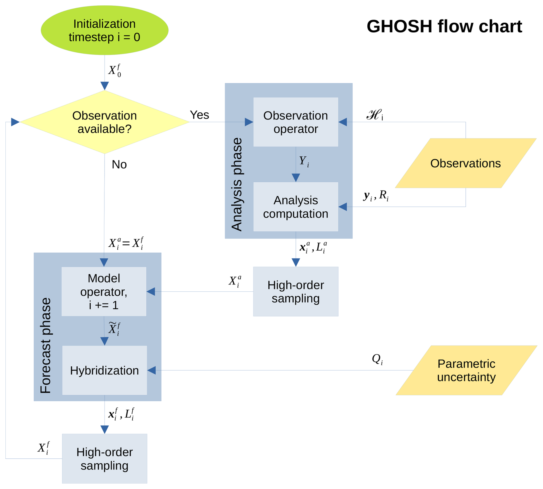
Figure 2 GHOSH filter flow chart. Subscripts represent the time steps of the numerical simulation.

The analysis equations are a novel weighted version of the ensemble Kalman filter equations (Evensen, 1994), while the forecast phase equations rely on a hybrid approach. In fact, the forecast uncertainty is obtained by combining the ensemble covariance (weighted by a forgetting factor) and a parametric covariance matrix Q_i, which is built from the existing knowledge of the system, as done, for instance, for the background matrix in many variational schemes (Bannister, 2017, 2008).

The method includes two resampling phases, after analysis and after forecast (Fig. 2), at which the whole ensemble is rebuilt using the high-order sampling method (Sect. 2). The resampling produces a sample of state vectors that matches the moments of the uncertainty probability density function with better precision than in the other commonly used ensemble DA algorithms, resulting in an order of approximation greater than 2 (see Appendix A) in the principal uncertainty modes. In this way the GHOSH filter takes advantage of the high approximation order of the sampling method twice: before applying the model operator and before applying the observation operator.

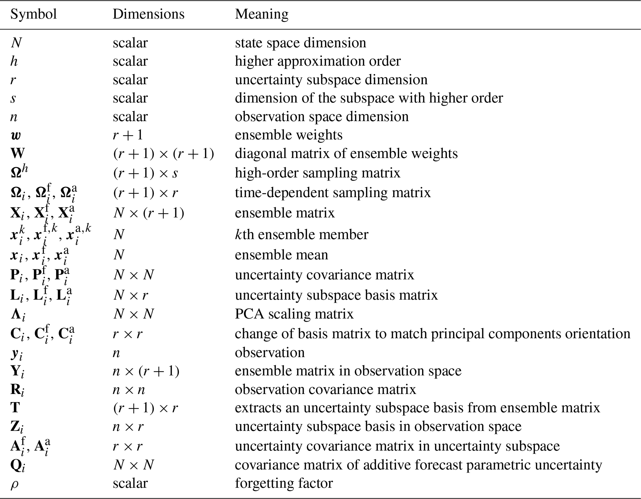
Table 1 helps taking track of symbols and notation.

Table 1 Notation table of the most relevant symbols.

3.1 The global GHOSH filter

3.1.1 Initialization

Based on the same hyper-parameters as the high-order sampling (Sect. 2.1.1), namely r (the dimension of the uncertainty subspace), h (the higher approximation order reached in the most relevant directions) and s (the number of principal components that are approximated with order h), GHOSH initialization computes the sampling matrix Ω^h and the weights vector w as in Sect. 2.1.2. Furthermore, a starting weighted ensemble must be provided, with the entries of w as weights. Such an ensemble can come from any previous forecast/assimilation using the GHOSH filter, or it can be built from scratch with an ensemble generation method (e.g., a PCA on historical data followed by the GHOSH sampling method described in Sect. 2.2). The ensemble members are stored in the columns of ensemble matrix ${\mathbf{X}}_{\mathrm{0}}^{\mathrm{f}}$, i.e.,

$$\begin{array}{}\text{(13)}& {\mathbf{X}}_{\mathrm{0}}^{\mathrm{f}}=\left({\mathit{x}}_{\mathrm{0}}^{\mathrm{f},\mathrm{1}},\mathrm{\dots },{\mathit{x}}_{\mathrm{0}}^{\mathrm{f},\left(r+\mathrm{1}\right)}\right),\end{array}$$

with the subscripted index 0 representing the first time step.

The mean ${\mathit{x}}_{\mathrm{0}}^{\mathrm{f}}$ can be computed as

$$\begin{array}{}\text{(14)}& {\mathit{x}}_{\mathrm{0}}^{\mathrm{f}}={\mathbf{X}}_{\mathrm{0}}^{\mathrm{f}}\mathit{w}.\end{array}$$

3.1.2 Analysis phase

When observations are available at time step i (Fig. 2), y_i∈ℝⁿ represents the observation array and ℋ_i is the observation operator, which incorporates all operations needed to obtain the observed quantities from the state vector. This operator is used on each ensemble member ${\mathit{x}}_i^{\mathrm{f},k}$ to build the $n\times \left(r+\mathrm{1}\right)$ matrix Y_i, i.e.,

$$\begin{array}{}\text{(15)}& {\mathbf{Y}}_i=\left({\mathit{y}}_i^{\mathrm{1}},\mathrm{\dots },{\mathit{y}}_i^{\left(r+\mathrm{1}\right)}\right),\end{array}$$

with

$$\begin{array}{}\text{(16)}& {\mathit{y}}_i^k={\mathcal{H}}_i\left({\mathit{x}}_i^{\mathrm{f},k}\right)\end{array}$$

for $k\in \left\{\mathrm{1},\mathrm{\dots },r+\mathrm{1}\right\}$.

The base ${\stackrel{\mathrm{̃}}{\mathbf{L}}}_i^{\mathrm{a}}$ of the uncertainty subspace spanned by the ensemble is computed by

$$\begin{array}{}\text{(17)}& {\stackrel{\mathrm{̃}}{\mathbf{L}}}_i^{\mathrm{a}}={\mathbf{X}}_i^{\mathrm{f}}\mathbf{T},\end{array}$$

where T is an $(r+\mathrm{1})\times r$ full-rank matrix with zero column sums. A matrix fulfilling these requirements, that also makes the product in Eq. (17) computationally fast, is

$$\begin{array}{}\text{(18)}& \mathbf{T}=\left(\begin{array}{ccc}& & \\ & {\mathbf{I}}_r& \\ & & \\ \mathrm{0}& \mathrm{\cdots }& \mathrm{0}\end{array}\right)-\mathit{w}{\mathbb{1}}_{\mathrm{1}\times r},\end{array}$$

with I_r being the identity matrix of size r and 𝟙 being a matrix (of the subscripted size) filled with ones. Equation (18) implies the use of the ensemble anomalies as basis members, and it is a common choice in SEIK implementations (e.g., Triantafyllou et al., 2003), but other Ts can be explored without affecting the main structure of the algorithm (see e.g., Nerger et al., 2012).

The analysis uncertainty covariance matrix ${\mathbf{P}}_i^{\mathrm{a}}$ is obtained by

$$\begin{array}{}\text{(19)}& {\mathbf{P}}_i^{\mathrm{a}}={\stackrel{\mathrm{̃}}{\mathbf{L}}}_i^{\mathrm{a}}{\mathbf{A}}_i^{\mathrm{a}}{{\stackrel{\mathrm{̃}}{\mathbf{L}}}_i^{\mathrm{a}}}^T,\end{array}$$

where

$$\begin{array}{}\text{(20)}& {\mathbf{A}}_i^{\mathrm{a}-\mathrm{1}}={\mathbf{T}}^T{\mathbf{W}}^{-\mathrm{1}}\mathbf{T}+{\mathbf{Z}}_i^T{\mathbf{R}}_i^{-\mathrm{1}}{\mathbf{Z}}_i,\end{array}$$

and

$$\begin{array}{}\text{(21)}& {\mathbf{Z}}_i={\mathbf{Y}}_i\mathbf{T},\end{array}$$

W=diag(w) being the $\left(r+\mathrm{1}\right)\times \left(r+\mathrm{1}\right)$ diagonal matrix of weights and R_i the n×n covariance matrix representing the uncertainty in the observation y_i.

An opportune change in basis is used to obtain the simpler decomposition

$$\begin{array}{}\text{(22)}& {\mathbf{P}}_i^{\mathrm{a}}={\mathbf{L}}_i^{\mathrm{a}}{{\mathbf{L}}_i^{\mathrm{a}}}^T,\end{array}$$

where

$$\begin{array}{}\text{(23)}& {\mathbf{L}}_i^{\mathrm{a}}={\stackrel{\mathrm{̃}}{\mathbf{L}}}_i^{\mathrm{a}}{\mathbf{S}}_i^{\mathrm{a}}\end{array}$$

and ${\mathbf{S}}_i^{\mathrm{a}}$ is the symmetric square root of ${\mathbf{A}}_i^{\mathrm{a}}$, i.e.,

$$\begin{array}{}\text{(24)}& {\mathbf{S}}_i^{\mathrm{a}}{\mathbf{S}}_i^{\mathrm{a}}={\mathbf{A}}_i^{\mathrm{a}}.\end{array}$$

Finally, the analysis state ${\mathit{x}}_i^{\mathrm{a}}$ is estimated by

$$\begin{array}{}\text{(25)}& {\mathit{x}}_i^{\mathrm{a}}={\mathit{x}}_i^{\mathrm{f}}+{\mathbf{L}}_i^{\mathrm{a}}{\mathbf{S}}_i^{\mathrm{a}}{\mathbf{Z}}_i^T{\mathbf{R}}_i^{-\mathrm{1}}\left({\mathit{y}}_i-{\mathbf{Y}}_i\mathit{w}\right).\end{array}$$

Equation (25) differs from the usual ensemble Kalman filter equations in the use of Y_iw in the last term instead of ${\mathcal{H}}_i\left({\mathit{x}}_i^{\mathrm{f}}\right)$. The two are the same if the observation operator ℋ_i is linear. However, in the general case, Y_iw, which relies on the whole ensemble instead of the ensemble mean only, is a better estimator of the expected value of the observed quantities. Moreover, ensembles generated with GHOSH's sampling method lead to a further advantage due to the higher order of approximation.

3.1.3 Analysis high-order sampling

The $N\times \left(r+\mathrm{1}\right)$ ensemble matrix ${\mathbf{X}}_i^{\mathrm{a}}=\left({\mathit{x}}_i^{\mathrm{a},\mathrm{1}},\mathrm{\dots },{\mathit{x}}_i^{\mathrm{a},\left(r+\mathrm{1}\right)}\right)$, whose columns are the ensemble members, is obtained by

$$\begin{array}{}\text{(26)}& {\mathbf{X}}_i^{\mathrm{a}}={\mathit{x}}_i^{\mathrm{a}}{\mathbb{1}}_{\mathrm{1}\times \left(r+\mathrm{1}\right)}+{\mathbf{L}}_i^{\mathrm{a}}{{\mathbf{C}}_i^{\mathrm{a}}}^T{{\mathbf{\Omega }}_i^{\mathrm{a}}}^T{\mathbf{W}}^{-\frac{\mathrm{1}}{\mathrm{2}}}.\end{array}$$

The sampling procedure is described in Sect. 2.2; therefore, ${\mathbf{C}}_i^{\mathrm{a}}$ and ${\mathbf{\Omega }}_i^{\mathrm{a}}$ are computed as C_i and Ω_i used in Eq. (6).

3.1.4 Forecast phase

In this phase, the time step index i is increased by 1 and the ensemble is evolved through the model operator ℳ_i (which usually represents the numerical integration of a system of differential equations), i.e., for $k\in \left\{\mathrm{1},\mathrm{\dots },r+\mathrm{1}\right\}$,

$$\begin{array}{}\text{(27)}& {\displaystyle }{\stackrel{\mathrm{̃}}{\mathit{x}}}_i^{\mathrm{f},k}={\mathcal{M}}_i\left({\mathit{x}}_{i-\mathrm{1}}^{\mathrm{a},k}\right),\text{(28)}& {\displaystyle }{\stackrel{\mathrm{̃}}{\mathbf{X}}}_i^{\mathrm{f}}=\left({\stackrel{\mathrm{̃}}{\mathit{x}}}_i^{\mathrm{f},\mathrm{1}},\mathrm{\dots },{\stackrel{\mathrm{̃}}{\mathit{x}}}_i^{\mathrm{f},\left(r+\mathrm{1}\right)}\right).\end{array}$$

The forecast state ${\mathit{x}}_i^{\mathrm{f}}$ is estimated as the weighted mean of the ensemble by

$$\begin{array}{}\text{(29)}& {\mathit{x}}_i^{\mathrm{f}}={\stackrel{\mathrm{̃}}{\mathbf{X}}}_i^{\mathrm{f}}\mathit{w}.\end{array}$$

To track the uncertainty of this estimation, the basis of the uncertainty subspace is obtained by

$$\begin{array}{}\text{(30)}& {\stackrel{\mathrm{̃}}{\mathbf{L}}}_i^{\mathrm{f}}={\stackrel{\mathrm{̃}}{\mathbf{X}}}_i^{\mathrm{f}}\mathbf{T}.\end{array}$$

The covariance matrix ${\mathbf{P}}_i^{\mathrm{f}}$ is approximated by

$$\begin{array}{}\text{(31)}& {\mathbf{P}}_i^{\mathrm{f}}={\stackrel{\mathrm{̃}}{\mathbf{L}}}_i^{\mathrm{f}}{\left({\mathbf{T}}^T{\mathbf{W}}^{-\mathrm{1}}\mathbf{T}\right)}^{-\mathrm{1}}{{\stackrel{\mathrm{̃}}{\mathbf{L}}}_i^{\mathrm{f}}}^T+{\mathbf{Q}}_i\approx {\stackrel{\mathrm{̃}}{\mathbf{L}}}_i^{\mathrm{f}}{\mathbf{A}}_i^{\mathrm{f}}{{\stackrel{\mathrm{̃}}{\mathbf{L}}}_i^{\mathrm{f}}}^T,\end{array}$$

where Q_i is the N×N covariance matrix of an additive unbiased noise parameterizing some of the sources of uncertainty in the forecast estimation not already accounted for by the ensemble, while ${\mathbf{A}}_i^{\mathrm{f}}$ is the r×r matrix approximating the uncertainty covariance in the reduced basis expressed by ${\stackrel{\mathrm{̃}}{\mathbf{L}}}_i^{\mathrm{f}}$. ${\mathbf{A}}_i^{\mathrm{f}}$ can be computed in many ways, depending on the form of Q_i and on the chosen hybridization strategy. Here we consider the case of Q_i being a full rank matrix (e.g., diagonal), thus we suggest

$$\begin{array}{}\text{(32)}& {\mathbf{A}}_i^{\mathrm{f}}={\left(\mathit{\rho }{\mathbf{T}}^T{\mathbf{W}}^{-\mathrm{1}}\mathbf{T}\right)}^{-\mathrm{1}}+{\left({{\stackrel{\mathrm{̃}}{\mathbf{L}}}_i^{\mathrm{f}}}^T{\mathbf{Q}}_i^{-\mathrm{1}}{\stackrel{\mathrm{̃}}{\mathbf{L}}}_i^{\mathrm{f}}\right)}^{-\mathrm{1}},\end{array}$$

where ρ is the forgetting factor, which is added to the equation to introduce inflation (see e.g., Pham et al., 1998; Anderson, 2007). The last term in Eq. (32) is one of the novel elements of the present work. It represents the projection of the parametric uncertainty matrix Q_i on the uncertainty subspace defined by the ensemble. While the use of Q_i in Eq. (31) follows Pham (2001), Eq. (32) projects Q_i in a novel non-orthogonal way that is induced by the scalar product defined by ${\mathbf{Q}}_i^{-\mathrm{1}}$. This approach can be interpreted as a form of hybridization that aims at focusing on the effects of the parametric uncertainty in the ensemble uncertainty subspace.

Q_i should be built according to some knowledge of the system, as done, for example, for the background covariance matrix in variational methods (Bannister, 2017, 2008). Since Q_i can have a very large size, it should be sparse or managed in a decomposed form.

Finally, Eq. (31) is conveniently rewritten as

$$\begin{array}{}\text{(33)}& {\mathbf{P}}_i^{\mathrm{f}}\approx {\mathbf{L}}_i^{\mathrm{f}}{{\mathbf{L}}_i^{\mathrm{f}}}^T,\end{array}$$

providing a covariance decomposition consistent with the high-order sampling formulation. Here, ${\mathbf{L}}_i^{\mathrm{f}}$ is the new basis of the uncertainty subspace and it is obtained by

$$\begin{array}{}\text{(34)}& {\mathbf{L}}_i^{\mathrm{f}}={\stackrel{\mathrm{̃}}{\mathbf{L}}}_i^{\mathrm{f}}{\mathbf{S}}_i^{\mathrm{f}},\end{array}$$

where ${\mathbf{S}}_i^{\mathrm{f}}$ is the symmetric square root of ${\mathbf{A}}_i^{\mathrm{f}}$, i.e.,

$$\begin{array}{}\text{(35)}& {\mathbf{S}}_i^{\mathrm{f}}{\mathbf{S}}_i^{\mathrm{f}}={\mathbf{A}}_i^{\mathrm{f}},\end{array}$$

which can be computed by an eigenvalue decomposition of ${\mathbf{A}}_i^{\mathrm{f}}$.

3.1.5 Forecast high-order sampling

The $N\times \left(r+\mathrm{1}\right)$ ensemble matrix ${\mathbf{X}}_i^{\mathrm{f}}=\left({\mathit{x}}_i^{\mathrm{f},\mathrm{1}},\mathrm{\dots },{\mathit{x}}_i^{\mathrm{f},\left(r+\mathrm{1}\right)}\right)$, whose columns are the ensemble members, is obtained by

$$\begin{array}{}\text{(36)}& {\mathbf{X}}_i^{\mathrm{f}}={\mathit{x}}_i^{\mathrm{f}}{\mathbb{1}}_{\mathrm{1}\times \left(r+\mathrm{1}\right)}+{\mathbf{L}}_i^{\mathrm{f}}{{\mathbf{C}}_i^{\mathrm{f}}}^T{{\mathbf{\Omega }}_i^{\mathrm{f}}}^T{\mathbf{W}}^{-\frac{\mathrm{1}}{\mathrm{2}}}.\end{array}$$

The sampling procedure is similar to that of Sect. 3.1.3; therefore, ${\mathbf{C}}_i^{\mathrm{f}}$ and ${\mathbf{\Omega }}_i^{\mathrm{f}}$ are computed as C_i and Ω_i used in Eq. (6).

Compared to data assimilation schemes with resampling only after analysis, the GHOSH filter uses this sampling phase to produce a better representation of the uncertainty.

In fact, it takes into account the effects of Q_i and ρ in Eqs. (31) and (32), which, by augmenting the uncertainty after the forecast, modify the second-order moments of the uncertainty pdf. Without this resampling, the forecast ensemble would no longer be either a high-order or a second-order sampling, since the ensemble does not match the changed covariance anymore. However, if Q_i is supposed to be not significant (i.e., Q_i=0) then the covariance is only modified by the forgetting factor ρ and the forecast high-order sampling phase can be widely simplified: in this specific case, indeed, the ensemble members can be safely obtained by inflating the ensemble anomalies, i.e.,

$$\begin{array}{}\text{(37)}& {\mathit{x}}_i^{\mathrm{f},k}={\mathit{x}}_i^{\mathrm{f}}+{\displaystyle \frac{\mathrm{1}}{\sqrt{\mathit{\rho }}}}\left({\stackrel{\mathrm{̃}}{\mathit{x}}}_i^{\mathrm{f},k}-{\mathit{x}}_i^{\mathrm{f}}\right),\end{array}$$

for $k\in \left\{\mathrm{1},\mathrm{\dots },r+\mathrm{1}\right\}$.

3.1.6 Asymptotic computational complexity

In order to assess the scaling capability of the proposed algorithm, this section presents the asymptotic computational complexity of the GHOSH filter. The estimate does not include the cost of applying the model operator ℳ_i and the observation operator ℋ_i. These operators can dramatically change the total computational cost, in particular in realistic applications, where the model operator can be very computationally expensive.

Further, the initialization cost is not taken into account, since it is done only once. This includes the computational cost of solving system (2), which can substantially vary depending on the adopted method. For instance, in the provided python code (see the Code availability section), an analytical solution for system (2) is built with a constructive method in 𝒪(r²) steps.

Finally, the covariance matrices ${\mathbf{Q}}_i^{-\mathrm{1}}$ and ${\mathbf{R}}_i^{-\mathrm{1}}$ and the scaling matrix ${\mathbf{\Lambda }}_i^{-\mathrm{1}}$ are considered sparse or low rank, such that, for instance, the computational complexity of ${\mathbf{Z}}_i^T{\mathbf{R}}_i^{-\mathrm{1}}{\mathbf{Z}}_i$ is the same as ${\mathbf{Z}}_i^T{\mathbf{Z}}_i$.

Under these assumptions, the most expensive operations in the analysis phase are: the computation of ${\mathbf{A}}_i^{\mathrm{a}-\mathrm{1}}$ (which is 𝒪(nr²)) and of its inverse (𝒪(r³)), and the change of basis of Eq. (23), which is a 𝒪(Nr²) operation. Excluding the cost of the observation operator ℋ_i, the analysis computational complexity sums to $\mathcal{O}\left(n{r}^{\mathrm{2}}+r^{\mathrm{3}}+N{r}^{\mathrm{2}}\right)$.

During the forecast phase, the computation of ${\mathbf{A}}_i^{\mathrm{f}}$ and the following change of basis (Eq. 34) lead to 𝒪(r³+Nr²), without taking into account the cost of the model operator ℳ_i.

Finally, each sampling phase adds 𝒪(r³+Nr²) operations given the eigenvalue decomposition and the matrix products in Eq. (6).

All together, the asymptotic computational complexity of the GHOSH filter is $\mathcal{O}\left(n{r}^{\mathrm{2}}+r^{\mathrm{3}}+N{r}^{\mathrm{2}}\right)$. This is similar to SEIK and ETKF (see, e.g., Nerger et al., 2012; Tippett et al., 2003), meaning that the filters scale in the same way. However, even if not changing the asymptotic complexity, the GHOSH filter's eigenvalue decomposition and its re-sampling after forecast are GHOSH-specific operations that add computational time with respect to other ensemble filters that do not execute such operations. On the other hand, in the vast majority of realistic geoscience applications of ensemble data assimilation, the most demanding computational cost is represented by the model integration scaled by the ensemble size (see e.g., Vetra-Carvalho et al., 2018), making the cost of the other data assimilation operations almost negligible.

3.2 The local GHOSH filter

Localization is a widely used procedure that aims to avoid spurious correlations induced by an overly small ensemble while reducing the degrees of freedom of the system (see e.g., Janjic et al., 2011).

A localized version of the GHOSH algorithm is obtained by modifying some of the equations in Sect. 3.1.2 and 3.1.4. Three operators ℒ_p, ${\mathcal{L}}_p^{\mathcal{H}}$ and 𝒟 are used to improve readability. The localization operator ℒ_p takes a global (array or) matrix with N rows and returns its localized counterpart with l rows with respect to the domain point p. The simplest and most common example of localization operator is taking just the variable values of the cells in a small radius around p. ${\mathcal{L}}_p^{\mathcal{H}}$ works in the same way in the observation space, reducing the number of rows from n to l^′. The delocalization operator 𝒟 takes a set of local matrices (or arrays), ideally one for each point of the domain, and returns the global counterpart. Building the global matrix by taking the values at the central points of each local matrix is a common example of delocalization operator.

3.2.1 Local forecast

Instead of Eqs. (31)–(35), the localized version of the forecast step of the algorithm computes, for each point p of the domain, the local covariance matrix ${\mathbf{A}}_i^{p,\mathrm{f}}$ by

$$\begin{array}{}\text{(38)}& \begin{array}{rl}{\mathbf{A}}_i^{p,\mathrm{f}}& ={\left(\mathit{\rho }{\mathbf{T}}^T{\mathbf{W}}^{-\mathrm{1}}\mathbf{T}\right)}^{-\mathrm{1}}+\\ & +{\left({\mathcal{L}}_p{\left({\stackrel{\mathrm{̃}}{\mathbf{L}}}_i^{\mathrm{f}}\right)}^T{\left({\mathbf{Q}}_i^p\right)}^{-\mathrm{1}}{\mathcal{L}}_p\left({\stackrel{\mathrm{̃}}{\mathbf{L}}}_i^{\mathrm{f}}\right)\right)}^{-\mathrm{1}},\end{array}\end{array}$$

where ${\mathbf{Q}}_i^p$ is the l×l covariance matrix at the point p of the parametric uncertainty non-dependent on the ensemble.

The global basis is built by changing the basis and delocalizing, i.e.,

$$\begin{array}{}\text{(39)}& {\mathbf{L}}_i^{\mathrm{f}}=\mathcal{D}\left({\left\{{\mathcal{L}}_p\left({\stackrel{\mathrm{̃}}{\mathbf{L}}}_i^{\mathrm{f}}\right){\mathbf{S}}_i^{p,\mathrm{f}}\right\}}_p\right),\end{array}$$

where ${\mathbf{S}}_i^{p,\mathrm{f}}$ is the symmetric square root of ${\mathbf{A}}_i^{p,\mathrm{f}}$. Note that the change in basis induced by ${\mathbf{S}}_i^{p,\mathrm{f}}$ is continuous (see, e.g., Nerger et al., 2012); thus, the delocalization operator does not need to include averaging or other smoothing procedures to avoid discontinuities.

3.2.2 Local analysis

The localized version of the analysis step substitutes Eqs. (19) and (20) by calculating, for each point p of the domain, the local covariance matrix ${\mathbf{A}}_i^{p,\mathrm{a}}$, i.e.,

$$\begin{array}{}\text{(40)}& {\mathbf{A}}_i^{p,\mathrm{a}-\mathrm{1}}={\mathbf{T}}^T{\mathbf{W}}^{-\mathrm{1}}\mathbf{T}+{\mathcal{L}}_p^{\mathcal{H}}{\left({\mathbf{Z}}_i\right)}^T{\left({\mathbf{R}}_i^p\right)}^{-\mathrm{1}}{\mathcal{L}}_p^{\mathcal{H}}\left({\mathbf{Z}}_i\right),\end{array}$$

where ${\mathbf{R}}_i^p$ is the $l^{\prime }\times l^{\prime }$ observation uncertainty covariance matrix at the point p. This matrix can be extracted from ${\mathbf{R}}_i^{-\mathrm{1}}$, but it is convenient to increase the uncertainty at the points far from p (as in Nerger and Gregg, 2007). One widely used option is to rescale by applying the fifth-order piecewise rational function of Gaspari and Cohn (1999).

Similarly to Eq. (39) for local forecast, Eq. (23) becomes

$$\begin{array}{}\text{(41)}& {\mathbf{L}}_i^{\mathrm{a}}=\mathcal{D}\left({\left\{{\mathcal{L}}_p\left({\stackrel{\mathrm{̃}}{\mathbf{L}}}_i^{\mathrm{a}}\right){\mathbf{S}}_i^{p,\mathrm{a}}\right\}}_p\right),\end{array}$$

where ${\mathbf{S}}_i^{p,\mathrm{a}}$ is the symmetric square root of ${\mathbf{A}}_i^{p,\mathrm{a}}$.

Finally, the analysis state ${\mathit{x}}_i^{\mathrm{a}}$ in Eq. (25) is instead estimated by

$$\begin{array}{}\text{(42)}& \begin{array}{rl}{\mathit{x}}_i^{\mathrm{a}}& ={\mathit{x}}_i^{\mathrm{f}}+\mathcal{D}\left(\mathit{\right\{}{\mathcal{L}}_p\left({\stackrel{\mathrm{̃}}{\mathbf{L}}}_i^{\mathrm{a}}\right){\mathbf{A}}_i^{p,\mathrm{a}}{\mathcal{L}}_p^{\mathcal{H}}{\left({\mathbf{Z}}_i\right)}^T\cdot \\ & \cdot {\left({\mathbf{R}}_i^p\right)}^{-\mathrm{1}}{\mathcal{L}}_p^{\mathcal{H}}\left({\mathit{y}}_i-{\mathbf{Y}}_i\mathit{w}\right){\mathit{\}}}_p).\end{array}\end{array}$$

4 Experimental setup

The GHOSH filter has been tested in a very large set of twin experiments based on the Lorenz96 model (Lorenz, 1996) to evaluate the performance of GHOSH compared with a second-order filter (SEIK). The Lorenz96 model, which has a chaotic behaviour that is comparable to that of fluid dynamics equations at a much lower computational cost, is a standard choice for testing new data assimilation schemes (e.g., Brajard et al., 2020; Fertig et al., 2007; Gharamti, 2018; Grooms and Robinson, 2021; Nerger, 2022).

In each experiment, the truth trajectory is provided by integrating the model for a certain time interval. Then, at regular time intervals, observations of a subset of the system variables have been extracted from the truth, adding a random error to each of them to represent the observation uncertainty. The same set of observations is then used for two assimilation experiments, one using the SEIK filter (as a second-order approximation filter Nerger et al., 2005), and one using the GHOSH filter with fifth-order approximation (i.e., h=5, see Sect. 3). The SEIK and GHOSH assimilation experiments are initialized with the same initial condition, chosen randomly around the truth initial condition. After an initial spin-up of 10 time units, the skill of each filter is evaluated by computing, during the whole simulation, the root mean square error (RMSE) between the filter forecast and the truth before the assimilation step. Representing both how often and how far the filters deviate from the truth, RMSE is a common proxy for filter skill. In the experiments, the RMSEs on assimilated and non-assimilated variables have been evaluated for each filter. Separately assessing filter skills on non-assimilated variables provides indications on the capability of transferring information gathered with observations to the whole state of the system, exploiting correlations.

In order to produce reliable statistics, the same procedure has been repeated 90 000 times varying the truth trajectory, the observations, the filters' initial conditions and some filters hyper-parameters such as the ensemble size and the forgetting factor.

4.1 The Lorenz96 model

The Lorenz96 model (Lorenz, 1996) is a dynamical system commonly used as a testing framework in data assimilation. The state vector $\mathit{x}=\left(x_{\mathrm{1}},\mathrm{\dots },x_N\right)\in {\mathbb{R}}^N$ is evolved according to the system of differential equations given by, for $\mathrm{1}\le j\le N$,

$$\begin{array}{}\text{(43)}& {\displaystyle \frac{\mathrm{d}{x}_j}{\mathrm{d}t}}=\left(x_{j+\mathrm{1}}-x_{j-\mathrm{2}}\right)x_{j-\mathrm{1}}-x_j+F,\end{array}$$

with periodic conditions, i.e., $x_{-\mathrm{1}}=x_{N-\mathrm{1}}$, x₀=x_N and $x_{N+\mathrm{1}}=x_{\mathrm{1}}$. In our implementation, the size of the state vector is N=62 and the forcing term is F=8, which is a common value used to generate chaotic behaviour.

The equations have been implemented in python and numerically solved using SciPy's solve_ivp routine with its default solver method (i.e., RK45).

At time t=0, the state vector has been initialized by adding a small perturbation (x_N=0.01) to the null solution x=0. The model has been integrated for 20 time units as spin-up, then, the following 1000 time units have been used as historical data to compute the climatological mean and covariance (performing a PCA on 10 000 snapshots taken every 0.1 time units). The model has been further integrated for other 20 time units of spin-up, followed by 80 time units, divided into 4 blocks of 20 time units. The model trajectory of each one of these 4 blocks has been taken as reference in a set of twin experiments and referred to as truth. In the same way, a longer block of 150 time units has been used as truth in a set of twin experiments aimed at testing long-run performances.

4.2 Observations

Observations are generated for each truth trajectory by extracting from the state vector the values of the even-indexed variables (i.e., $x_{\mathrm{2}},x_{\mathrm{4}},\mathrm{\dots },x_{\mathrm{62}}$) every Δt time units and adding to each observed variable a random number sampled from a standard normal distribution (i.e., with variance equal to 1). Tests have been carried out for $\mathrm{\Delta }t\in \left\{\mathrm{0.1},\mathrm{0.15},\mathrm{0.2},\mathrm{0.25},\mathrm{0.3}\right\}$.

4.3 Filters setup

The same settings are used in both SEIK and GHOSH filters. The ensemble size is chosen among 7, 15, 31 and 63 members.

The initial condition of the ensemble mean is chosen randomly around a truth initial condition, adding a random Gaussian noise with 0-mean and same covariance matrix as the climatological covariance of the Lorenz96 model (Sect. 4.1). The initial ensemble is sampled with each filter's own sampling method (second-order-exact sampling for SEIK, high-order sampling with h=5 for GHOSH), setting the prior covariance matrix accordingly to the PCA approximation of the climatological covariance (i.e., r principal components are taken into account if the ensemble size is r+1).

Both filters use the same forgetting factor (Eq. 32), chosen among $\mathrm{0.5},\mathrm{0.55},\mathrm{0.6},\mathrm{0.65},\mathrm{0.7},\mathrm{0.75},\mathrm{0.8},\mathrm{0.85},\mathrm{0.9},\mathrm{0.95}$ and 1 (the last value describes a condition without inflation). The GHOSH filter is run without hybridization (Q_i=0) to keep GHOSH and SEIK as similar as possible, and Λ_i is the identity matrix.

The order of the GHOSH filter was fixed at h=5, with s (i.e., the number of principal components approximated with order h=5) as large as possible, depending on the ensemble size. Hence, the values adopted for s are $\mathrm{2},\mathrm{3},\mathrm{4}$ and 5, respectively, for $\mathrm{7},\mathrm{15},\mathrm{31}$ and 63 ensemble members.

Localization has not been applied, since the number of variables N is relatively small and comparable with the ensemble size.

4.4 Experimental design

The twin experiments have been performed in two phases, the first one for the 20-time-unit-long truth trajectories and the second one for the 150-time-unit-long trajectory. The relatively short time series in the first experiment phase are motivated by the aim to focus on comparing DA convergence after the assimilation and not on long-term convergence. On the other hand, the 150-time-unit experiments have been carried out to verify the robustness of the filter on longer time scales.

In the first phase, for each of the 4 20-time-unit-long truth trajectories, 100 twin experiments have been launched for each of the 5 observation frequencies, 4 ensemble sizes and 11 forgetting factors (for a total of 88 000 twin experiments). Each of the 100 twin experiments has its own set of random observations and initial conditions.

The RMSE score of the first phase experiments has been used to identify the best forgetting factor for each filter in each configuration of observation frequency and ensemble size. Then, in the second phase, the 150-time-unit-long truth trajectory has been employed in a set of 100 twin experiments for each of the 5 observation frequencies and 4 ensemble sizes (for a total of 2000 longer twin experiments), using for each filter its best forgetting factor in each configuration.

All the code was written in python and executed on a Linux computer equipped with an Intel(R) Core(TM) i7-11800H @2.30GHz.

5 Results

5.1 20-time-unit-long experiments

Figure 3 reports an example of the evolution of the first two variables (one assimilated and one non-assimilated) of the Lorenz96 model for the two filters (GHOSH and SEIK). The selected simulation out of 88 000 experiments shows that GHOSH filter evolution is closer to truth evolution (black line in Fig. 3) than SEIK. As expected, the uncertainty of variable 2 (shaded areas) of both filters is lower than in variable 1 because of the assimilation of observations in even variables.

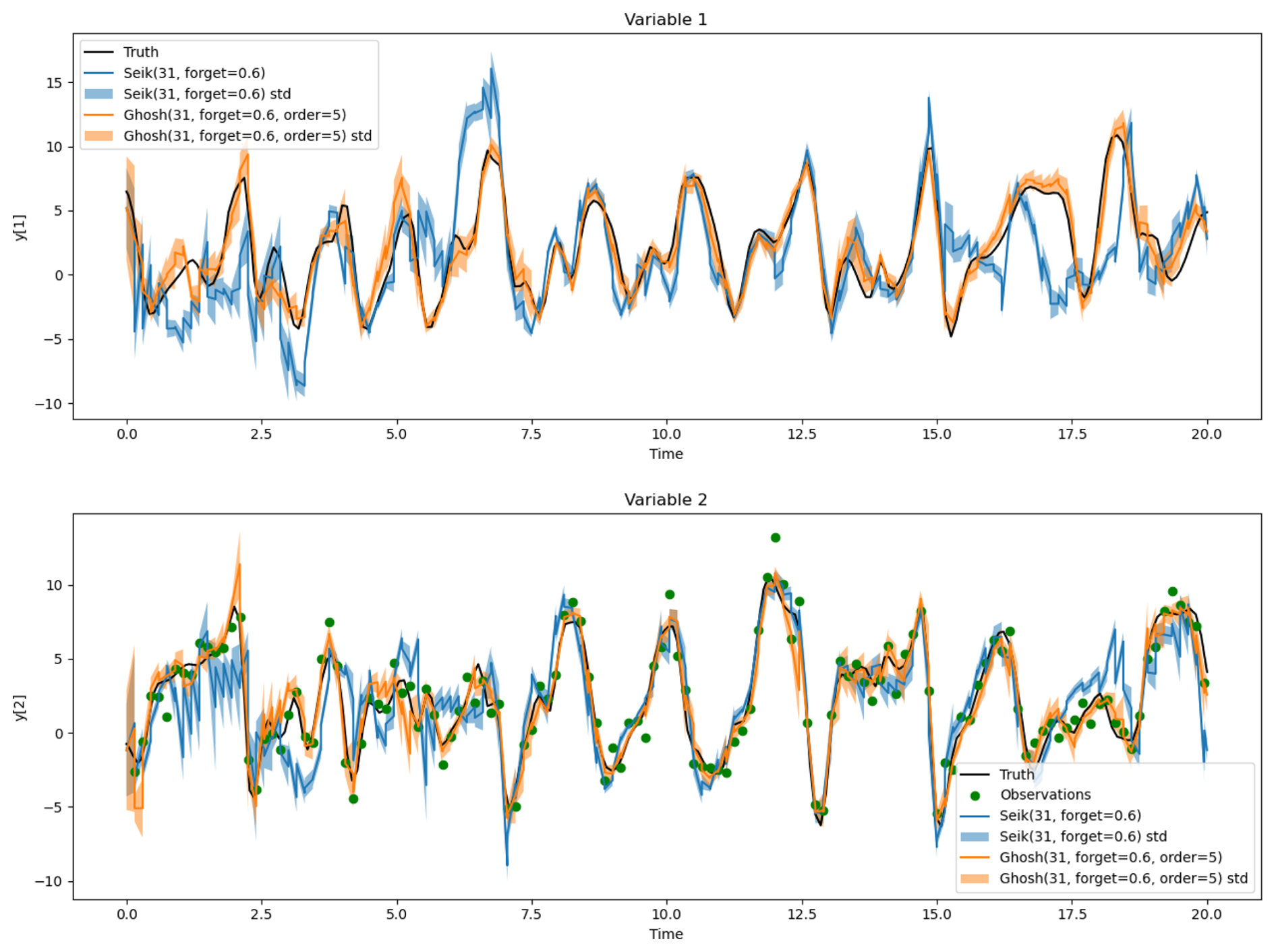
Figure 3 Results from one example twin experiment: time between observations (green dots) is 0.15, forgetting factor is 0.6, ensemble size is 31. Shady areas around blue (SEIK) and orange (GHOSH) lines represent the ensemble standard deviation, truth is the black line. Top panel: time evolution of the first variable (non-assimilated); bottom panel: time evolution of the second variable (assimilated).

Figure 4 Result summary of 20-time-unit-long twin experiments: each square in the colour-maps represents the aggregated results of 400 twin experiments, changing truth, observations and initial conditions. The results are summarized with colour-maps aggregated in six different rows, from top to bottom: SEIK RMSE of assimilated variables, SEIK RMSE of non-assimilated variables, GHOSH RMSE of assimilated variables, GHOSH RMSE of non-assimilated variables, the ratio of GHOSH RMSE over SEIK RMSE of assimilated variables, the ratio of GHOSH RMSE over SEIK RMSE of non-assimilated variables (red color implies that GHOSH is better than SEIK). Each column of colour-maps has different observation frequency, with the numbers on the top indicating the time elapsed between each observation/assimilation. Each colour-map shows different forgetting factors (Forget, along the y axis) and ensemble sizes (EnsSize, along the x axis).

In order to be statistically reliable, the RMSE of the 88 000 experiments under different conditions has been computed and reported in aggregated form in Fig. 4. Each small square reports the RMSE value computed over a set of 400 experiments², which includes, for each of the four available truths, 100 experiments with different random observations and initial conditions. Aggregating 400 experiments together reduces the outcome variability by a factor 20 (i.e., $\sqrt{\mathrm{400}}$) with respect to a single twin experiment, removing stochasticity concerns in the analysis of the twin experiment results.

The first two rows of colour-maps refer to assimilated and non-assimilated variables for the SEIK filter. In each colour-map, the time interval between assimilated observations increases from left to right, while the different forgetting factor values decrease from top to bottom. The first line in each colour-map, labelled “best”, represents the best result, in terms of lowest RMSE, obtained among the set of tested forgetting factors (i.e., the skill of the filters when optimally tuned). The color scale is capped to an RMSE of 4, the climatological standard deviation of the model, that represents the threshold under which the filter performs a successful assimilation.

The GHOSH experiments are summarized in the same way in the 3rd and 4th rows of Fig. 4, while the last two rows show the ratio between GHOSH and SEIK RMSE values, with red color indicating RMSE reduction of GHOSH with respect to SEIK.

Figure 5 Example of a single twin experiment, with SEIK (blue line) showing diverging behaviour: time between observations (green dots) is 0.15, forgetting factor is 0.6, ensemble size is 31. Values over time of a non-assimilated (top) and an assimilated (bottom) variable.

The column corresponding to the smallest ensemble size (i.e., 7 members) is not shown, since in this case SEIK and GHOSH behave very similarly, with very poor performances, due to lack of capability of describing the system complexity with an overly small ensemble size.

The yellow 15-member columns also show poor performances in all configurations but, looking at the last two rows of Fig. 4, the GHOSH RMSE is significantly better than SEIK RMSE (red squares), specially for low values of forgetting factor. In fact, while the GHOSH filter keeps the RMSE around the climatological values, the SEIK filter is more prone to numerical divergence ending up on trajectories far from the truth (see Fig. 5 for an example of diverging behaviour).

Considering the cases with 31 and 63 ensemble members, the GHOSH filter produces a successful assimilation (i.e., achieving an RMSE smaller than the climatological standard deviation, which is represented in yellow in Fig. 4) in almost all configurations (except two yellow squares representing experiments without inflation in the case of observation interval smaller than 0.15 time units). The SEIK filter instead shows a more limited capacity to produce a successful assimilation, as proved by a larger number of yellow squares in Fig. 4. Remarkably, the GHOSH filter with 31 ensemble members improves the state estimation error compared to the climatological standard deviation of the model for every observation interval. The same is not true for the SEIK filter, which achieves convergence (i.e., RMSE lower than the climatological standard deviation, at least in its best forgetting factor configuration) only for observation intervals shorter than 0.2 time units.

Looking at the last two rows of Fig. 4, the GHOSH filter outperforms the SEIK filter in most conditions, up to a 3-times RMSE reduction. Furthermore, GHOSH is always at least as good as SEIK. In the range of explored forgetting factors, the largest improvements (dark red, RMSE ratio 0.30) mainly occur when: (i) inflation is low (forgetting factor close to 1), (ii) a large amount of information is injected into the assimilation scheme (i.e., high frequency observations, left side of Fig. 4), and (iii) the filter can take into account a high dimensional uncertainty subspace (i.e., the ensemble size is large).

On the other hand, the comparison of each filter tuned with its best forgetting factor (the “best” top line in each colour-map) clearly shows that the GHOSH filter has considerably better performance than the SEIK filter (up to an RMSE ratio of 0.44) with a moderate number of ensemble members (31). In case of maximum ensemble size the improvement is still significant but less intense (up to 0.90 RMSE ratio).

The first four lines of Fig. 4 make evident that the GHOSH filter, compared to SEIK, is less dependent on inflation, reaching its best performance with a forgetting factor closer to 1.

The skill of both filters is closely related with the observations frequency: the shorter the time between observations, the higher the accuracy.

Finally, as expected, for both filters the skill is better on assimilated variables than non-assimilated ones but, quite interestingly, the RMSE ratio shows that the GHOSH advantage over SEIK is slightly larger in all the non-assimilated variables compared to the assimilated ones with the same settings (up to 0.08 RMSE ratio improvement in the best forgetting factor configuration, from 0.69 for assimilated to 0.61 for non-assimilated variables).

5.2 150-time-unit-long experiments

Similarly to the case of the 20-time-unit-long twin experiments, the results of the 150-time-unit-long tests are summarized in Fig. 6. Each small square reports the RMSE value computed over a set of 100 experiments with different random observations and initial conditions. In the top panel, the 5 colour-maps correspond to different time intervals between observations, increasing from left to right. Each colour-map shows, for assimilated and non-assimilated variables and for different ensemble sizes, the RMSE of the SEIK filter. The RMSE of the GHOSH filter is represented in the same way in the middle panel, while the ratio of the GHOSH RMSE over SEIK RMSE is shown in the bottom panel.

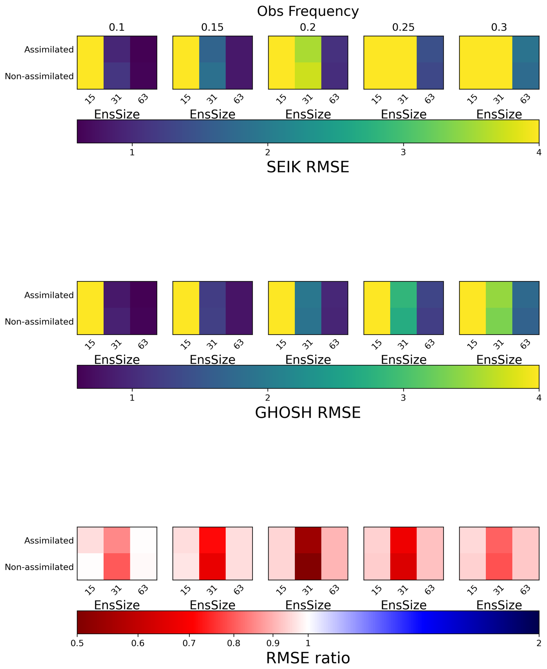
Figure 6 Result summary of 150-time-unit-long twin experiments: each square in the colour-maps represents the aggregated results of 100 twin experiments, changing observations and initial conditions. The results are summarized with colour-maps aggregated in 3 different rows, from top to bottom: SEIK RMSE, GHOSH RMSE, ratio of GHOSH RMSE over SEIK RMSE (red color implies that GHOSH is better than SEIK). Each column of colour-maps has different observation frequency, with the numbers on the top indicating the time elapsed between each observation/assimilation. Each colour-map shows, for assimilated and non-assimilated variables, different ensemble sizes (EnsSize, along the x axis).

The longer experiments confirm the result obtained by the shorter ones, with GHOSH performing better than SEIK in every configuration. In particular, the improvement is maximum (0.51 RMSE ratio) in the case of 31 ensemble members. Both filters show poor performance at 15 or fewer ensemble members, and both of them achieve a good convergence at the maximum ensemble size. In the case of 31 ensemble members, the behaviour of GHOSH and SEIK differs when the observation interval is 0.25 time units or longer, with GHOSH achieving a successful assimilation (blue-green color) while SEIK performs worse than the climatological error (yellow color).

The long-run experiments also confirm that the improvement is slightly larger for non-assimilated variables than for assimilated ones, scoring a better RMSE ratio (maximum ratio improvement of 0.05) in almost all configurations.

5.3 Computational cost

From the computational point of view, the whole experiment set required around 9 computational hours. SEIK and GHOSH schemes used 12 % and 16 % of the total time respectively, while the rest was devoted to model integration. Unexpectedly, the model integration time (averaged every 100 twin experiments) when applying the SEIK filter is sometimes longer than in the GHOSH filter case, up to twice as long, depending on some settings and random factors. This difference in computational time is more evident and occurs more often when the forgetting factor is lower (i.e., when the inflation is more pronounced). The reason can be understood by looking at Fig. 5: in this experiment with forgetting factor equal to 0.6, the SEIK filter presents an unstable and diverging behaviour. When it happens, the SciPy's solve_ivp integrating routine reduces the time step size to ensure the required accuracy, which comes with longer integration time.

Due to the increase in integration time when the filter is not converging, the percentage of computational time used by the filters with respect to the total time greatly varies from case to case, depending on the particular experiment parameters and on filter convergence. On average, in our experiments on the Lorenz96 model, the time to solution is dominated by the model integration and the difference between GHOSH and SEIK only accounts for 4 % of the total time. This difference between the two filters is explained by the fact that the GHOSH filter executes more operations than SEIK (mainly an eigenvalue decomposition) resulting in more computational time even if the asymptotic computational complexity of the two methods is the same (Sect. 3.1.6).

6 Discussion

The name “Gauss-Hermite high-order sampling hybrid filter” was chosen to indicate the two main features of this novel filter. First, it is a hybrid filter, in the sense that the uncertainty covariance matrix is obtained by averaging the ensemble covariance and a parametric covariance matrix non-depending on the ensemble, as described in, e.g., Carrassi et al. (2018). Second, it exploits a novel sampling method based on a Gauss-Hermite-like quadrature rule to reach an arbitrarily high (depending on the ensemble size) polynomial order of approximation.

The latter feature introduces, to the best of our knowledge, a completely new class of DA algorithms with an order of approximation higher than 2. The advantage of moving to a higher order of approximation has previously been documented in the literature, in particular Nerger et al. (2005) compares order 1 algorithms (e.g., SEEK Pham et al., 1998) and order 2 algorithms (e.g., SEIK Pham, 2001). The results of Sect. 5 confirm the expected benefits of the high-order sampling adopted in the GHOSH filter. In particular, in the Lorenz96 idealized and controlled conditions, the novel method outperforms (up to 56 % lower RMSE) a typical second-order method like SEIK and features higher stability and better performance.

Thanks to the large number of settings tested in the Lorenz96 twin experiment, it is possible to suggest the conditions where the GHOSH filter considerably increases the assimilation skill and reliability. Concerning the ensemble size, the larger improvements occur when the dimension of the uncertainty subspace spanned by the ensemble is large enough to be representative. If the number of ensemble members is too small, the assimilation simply fails independently of the tested assimilation algorithm, but even in that case, the GHOSH filter error is less detrimental than the SEIK error. Moreover, it has been shown that the GHOSH increased accuracy reduces instabilities and numerical divergence in our Lorenz96 implementation (Fig. 5). This aspect is consistent with the fact that a higher order of approximation helps to manage nonlinearities (Nerger et al., 2005). GHOSH filter showed a lower need for inflation with respect to SEIK, removing one of the instability causes observed in the twin experiment (Sect. 5). Indeed, in the twin experiment, a larger number of instability cases were observed at lower inflation values both for SEIK and GHOSH (one example with diverging SEIK is shown in Fig. 5). The lower need for inflation can be also seen as a GHOSH's improved capacity to take into account nonlinearity. Indeed, nonlinearity typically introduces errors that are not considered by ensemble filters, which need inflation to compensate for this uncertainty covariance underestimation (see e.g., Raanes et al., 2019; Bocquet et al., 2015; Rainwater and Hunt, 2013). Finally, the GHOSH filter could remarkably perform a successful assimilation even when the SEIK filter is failing due to observation sparsity.

Even if a large number of settings have been tested in the twin experiments, other Lorenz96 literature applications (see e.g., Brajard et al., 2020; Fertig et al., 2007; Gharamti, 2018; Grooms and Robinson, 2021; Grooms, 2022; Kirchgessner et al., 2014; Lei and Bickel, 2011; Nerger, 2022; Scheffler et al., 2022) tested ensemble DA methods applying different conditions and strategies. In particular, longer time series, different observation operators or different state vector dimensions have been considered. The shorter time series in the first experiment phase in the present work (Sect. 4.4) are motivated by the aim to focus on comparing DA convergence in the phase after the assimilation and not on long-term convergence. Thanks to this approach, our results provide information for possible realistic applications of GHOSH in geoscientific operational simulations. In this framework, the shown initial fast convergence of the GHOSH filter is strongly beneficial to improve the simulation accuracy on temporal scales of interest.

In addition to a higher polynomial order, the GHOSH filter features a resampling taking place twice per step. Ensemble Kalman-like filters usually adopt an interpolation strategy by applying the observation operator directly to the ${\stackrel{\mathrm{̃}}{\mathbf{X}}}_i^{\mathrm{f}}$ ensemble of the states after the model evolution (see Eq. 28). However, this strategy might lead to inaccurate estimations because the covariance matrix Q_i of Eq. (31) is not taken into account in the interpolation. For this reason, if Q_i is not zero, GHOSH applies the observation operator to a new ensemble, resampled between the forecast and analysis phases (Fig. 2). In this way, Q_i is taken into account and, especially in the case of a nonlinear observation operator, the high order of the sampling method is exploited to improve the accuracy of the projection into the observation space (as in Part 2,  Spada et al., 2026).

The statistical moments μ in Eq. (2) are key hyper-parameters that describe the uncertainty pdf moments for orders higher than 2. In our experiments we used the moments of a Gaussian distribution, but it is worth noting that the GHOSH algorithm does not enforce this choice and other pdfs could be used. However, Kalman filter analysis equations somehow prescribe a Gaussian approximation, thus the GHOSH filter keeps a link to Gaussianity, even if the GHOSH sampling does not. Interestingly, other filters, like Hodyss (2011), try to overcome this limitation and could represent good candidates to study the effects of a non-Gaussian GHOSH sampling.

The scaling matrix Λ_i used in the sampling procedure plays an important role in the filter, since Λ_i defines how variables are compared to each other in the computation of the most relevant components of the state uncertainty (Eq. 7). In the Lorenz96 case, it is straightforward to set Λ_i equal to the identity matrix, since each variable is equivalent to any other. In more complex applications, Λ_i should be carefully designed to focus on the variables relevant for the processes of interest (see also Spada et al., 2026, for a non-identity Λ_i and further discussion).

In the present implementation, the GHOSH filter derives the uncertainty subspace basis (Eq. 17) using a T matrix (Eq. 18) inherited from the SEIK filter. This is an advantage from the computational point of view, but ensemble members after the resampling may be very different from the original ensemble. For this reason, in some applications issues can arise, for instance, in the case of the physical balance constraints. As a solution, Nerger et al. (2012) propose a filter (the error subspace transform Kalman filter, ESTKF) that, during the analysis step, minimizes the unnecessary changes to the forecast ensemble, and such approach can also be applied to the GHOSH filter algorithm by choosing an appropriately designed T matrix. However, differently from the ESTKF case, the T matrix should change at every forecast to take into account GHOSH projections onto the principal components of the uncertainty subspace, introducing an additional complexity layer to the newly presented GHOSH filter. Thus, given the additional complexity of the ESTKF approach and considering that: (i) its effects are less important if the state vector does not strongly need to preserve specific nonlinear constrains; (ii) Nerger et al. (2012) showed that, in Lorenz96, SEIK with random rotation (adopted also in GHOSH) is as good as ESTKF; in the present work we limited to adopting a GHOSH filter that relies on a SEIK-like approach.

Compared to other ensemble filters, the key feature of the GHOSH filter is the higher polynomial order of its sampling method. The advantage of a higher order is not limited to a better estimation of the mean state (Appendix A) but it extends to the covariance matrix of the uncertainty probability distribution. In fact, the polynomial order in the estimation of the covariance matrix is half the order of the mean (not shown). Since the covariance matrix is involved in the state estimation, the more accurate GHOSH results shown in Sect. 5 can be partly related to an improvement in the approximation error affecting the uncertainty covariance matrix. Moreover, it is worth noting that a higher order of the sampling positively impacts the approximation of the nonlinearity of the model independently of its Gaussianity. The examples in Appendix C show how moments of order higher than two can affect a sampling of a Gaussian pdf. In fact, even if its first two moments completely characterize the distribution, the sampling needs to also match the higher moments to produce an ensemble capable of achieving an order of approximation higher than two.

Similarly to other ensemble filters, a weighted ensemble is used in the GHOSH filter. However, the GHOSH filter differs substantially from the particle filter (e.g., van Leeuwen et al., 2019) and from other types of weighted ensemble filters, e.g., Hoteit et al. (2008) and Stordal et al. (2011). In the listed filters, weights (representing likelihood) change over time, while particles remain the same (and strategies are applied to resample the particles when weights “collapse”, e.g., van Leeuwen et al., 2019). In the case of GHOSH, the ensemble is used to estimate specific moments and then resampled to keep the weights constant in time, because those weights have specific desired properties that help reduce the error of the mean estimation. In this, GHOSH has similarities with the nonlinear ensemble transform filter (Tödter and Ahrens, 2015), which does a resampling to keep the weights constant but, differently from GHOSH, with uniform weights and a second-order sampling procedure.

Finally, the asymptotic computational complexity of the GHOSH filter (Sect. 3.1.6) is comparable to second-order deterministic filters (e.g., SEIK, ETKF). In our experiments (Sect. 5.3), GHOSH showed an increased computational time with respect to SEIK (on average, 4 % of the total computational time), mainly due to the GHOSH filter's eigenvalue decomposition. However, it is worth noting that the cost related to the eigenvalue decomposition only depends on the number of ensemble members, affecting the 𝒪(r³) part of the full GHOSH complexity $\mathcal{O}\left(r^{\mathrm{3}}+\left(N+n\right)r^{\mathrm{2}}\right)$. As such, the eigenvalue decomposition is an important term if N+n (i.e., the sum of the dimensions of model and observations) is small (in our experiments on the Lorenz96 model it is smaller than 100), but becomes orders of magnitude less relevant in a realistic geoscience application, where degrees of freedom can be of the order of the millions and above. Moreover, while the model integration time and the filter computational time are still comparable in our experiments (12 % and 16 % for SEIK and GHOSH respectively), in a realistic application this will not be the case. Indeed, the filters computational complexity shows that filter computational time grows linearly with model dimension and the same holds for the Lorenz96 model that, however, is orders of magnitude less complex and computationally expensive than a realistic geoscience model. This is consistent with results obtained in a companion paper (Spada et al., 2026), where the GHOSH filter computational time in a realistic application accounts for less than 1 % of the total computational cost.

In summary, the benefits of the higher order offered by the GHOSH filter rely on a mathematical advantage with limited impacts on computational effort. In fact, GHOSH allows the exploitation of the degrees of freedom in the randomness of the sampling process, choosing ensembles that have a better consistency with the uncertainty distribution.

7 Conclusions

This work introduces two novel ensemble strategies: a sampling method (the high-order sampling) and an ensemble hybrid DA filter (GHOSH). Exploiting the high-order sampling, the GHOSH filter features a higher order of approximation compared to other ensemble filters, which resulted in better data assimilation performance.

Based on the results of the present work, the order of an ensemble method can be one of the proxies for filter skill, as shown by comparing SEIK (order 2) with GHOSH (order higher than 2).

While increasing the order usually involves increasing the number of ensemble members (and consequently the computational cost), the GHOSH approach keeps the same computational complexity and number of ensemble members as SEIK or ETKF and exploits the advantage of a higher order only where the approximation errors are larger.

In this work the validation and implementation of the GHOSH filter is limited to the Lorenz96 idealized setting, while the feasibility in a realistic geophysical application has been assessed in a companion paper (Spada et al., 2026) by testing a 3D parallel implementation of a Mediterranean physical-biogeochemical model.

The improvements of the GHOSH filter (in its non-hybrid version) with respect to the SEIK filter are demonstrated in an extensive set of twin experiments based on the Lorenz96 model. The GHOSH filter showed an improved capacity to take into account nonlinearities through a lower need for inflation with respect to SEIK, along with the capability of performing a successful assimilation even when observation sparsity was causing SEIK to fail. In every configuration, the GHOSH filter proved to be as good as SEIK or better. Considering each filter tuned with its optimal forgetting factor, the GHOSH filter significantly improved the assimilation skill with respect to SEIK, achieving its best RMSE reduction (56 %) in the setting with moderate ensemble size (31 members).

Appendix A: High-order sampling

Sampling a limited number of ensemble members that effectively represent the uncertainty of the state estimation is a crucial part of any ensemble algorithm. The GHOSH filter uses multi-dimensional Gauss-Hermite-like quadrature rules to choose the ensemble members, achieving a high polynomial order of convergence.

The core idea behind the GHOSH sampling can be proved by taking two independent random variables with the same moments up to a certain order h. Thus, they have the same mean after applying any polynomial function of degree at most h. In fact, given a probability density function (pdf) $p:{\mathbb{R}}^s\to \mathbb{R}$, if $\mathcal{F}:{\mathbb{R}}^s⟶\mathbb{R}$ is a polynomial function such that

$$\begin{array}{}\text{(A1)}& \mathcal{F}\left(\mathit{x}\right)=f_{\mathrm{0}}+\sum _{\mathit{\xi }=\mathrm{1}}^h\sum _{j_{\mathrm{1}},\mathrm{\dots },j_{\mathit{\xi }}=\mathrm{1}}^s{f}_{\mathit{\xi }}^{j_{\mathrm{1}},\mathrm{\dots },j_{\mathit{\xi }}}{x}_{j_{\mathrm{1}}}\mathrm{\cdots }{x}_{j_{\mathit{\xi }}},\end{array}$$

where s is the space dimension, $f_{\mathit{\xi }}^{j_{\mathrm{1}},\mathrm{\dots },j_{\mathit{\xi }}}$ are the polynomial coefficients and $x_{\mathrm{1}},\mathrm{\dots },x_s$ are the entries of x, then the mean $\stackrel{\mathrm{‾}}{\mathcal{F}}$,

$$\begin{array}{}\text{(A2)}& \begin{array}{rl}\stackrel{\mathrm{‾}}{\mathcal{F}}& =\underset{{\mathbb{R}}^s}{\int }\mathcal{F}\left(\mathit{x}\right)p\left(\mathit{x}\right)\mathrm{d}x=\\ & =f_{\mathrm{0}}+\sum _{\mathit{\xi }=\mathrm{1}}^h\sum _{j_{\mathrm{1}}=\mathrm{1}}^s\mathrm{\dots }\sum _{j_{\mathit{\xi }}=\mathrm{1}}^s{f}_{\mathit{\xi }}^{j_{\mathrm{1}},\mathrm{\dots },j_{\mathit{\xi }}}\underset{{\mathbb{R}}^s}{\int }{x}_{j_{\mathrm{1}}}\mathrm{\cdots }{x}_{j_{\mathit{\xi }}}p\left(\mathit{x}\right)\mathrm{d}\mathit{x},\end{array}\end{array}$$

depends only on the first h moments of the pdf p, which are represented by the last integral in Eq. (A2).

This proves that the mean of an operator can be computed exactly up to a certain order h by substituting the sampled probability distribution with any discrete finite probability distribution (such as a weighted ensemble) as long as their moments match (up to order h).

In order to build an ensemble with this property, the moment-matching equations are summarized by the nonlinear system

$$\begin{array}{}\text{(A3)}& \left\{\begin{array}{l}\mathrm{⋮}\\ {\displaystyle }\sum _{m=\mathrm{1}}^{r+\mathrm{1}}{x}_{j_{\mathrm{1}},m}\mathrm{\cdots }{x}_{j_{\mathit{\xi }},m}{w}_m={\mathit{\mu }}_{j_{\mathrm{1}},\mathrm{\dots },j_{\mathit{\xi }}},\\ \mathrm{⋮}\end{array}\right.\end{array}$$

with one equation for each $\mathit{\xi }\in \left\{\mathrm{0},\mathrm{\dots },h\right\}$ and for each $j_{\mathrm{1}},\mathrm{\dots },j_{\mathit{\xi }}\in \left\{\mathrm{1},\mathrm{\dots },s\right\}$.

In the system (A3), x_j,m is the jth entry of the mth ensemble member, r+1 is the ensemble size, w_m≥0 are the weights and ${\mathit{\mu }}_{j_{\mathrm{1}},\mathrm{\dots },j_{\mathit{\xi }}}$ are the statistical moments of p, i.e.,

$$\begin{array}{}\text{(A4)}& {\mathit{\mu }}_{j_{\mathrm{1}},\mathrm{\dots },j_{\mathit{\xi }}}=\underset{{\mathbb{R}}^s}{\int }{x}_{j_{\mathrm{1}}}\mathrm{\cdots }{x}_{j_{\mathit{\xi }}}p\left(\mathit{x}\right)\mathrm{d}\mathit{x}.\end{array}$$

The system is solved considering x_j,m and w_m as the unknowns, while p can be taken uncorrelated, normalized and with 0 mean without loss of generality. In fact, the ensemble matrix $\stackrel{\mathrm{̃}}{\mathbf{X}}=\left(x_{j,m}\right)$ (which contains in its columns the ensemble members with 0 mean and covariance matrix equal to the identity matrix I_s) can be transformed into the ensemble matrix X with arbitrary mean $\stackrel{\mathrm{‾}}{\mathit{x}}$ and covariance matrix LL^T through the projection

$$\begin{array}{}\text{(A5)}& \mathbf{X}=\stackrel{\mathrm{‾}}{\mathit{x}}{\mathbb{1}}_{\mathrm{1}\times \left(r+\mathrm{1}\right)}+\mathbf{L}\stackrel{\mathrm{̃}}{\mathbf{X}},\end{array}$$

where ${\mathbb{1}}_{\mathrm{1}\times \left(r+\mathrm{1}\right)}$ is a matrix (of the subscripted size) filled with ones.

As an example, in the special case of the standard normal distribution, i.e., p(x)=φ(x) is the pdf corresponding to 𝒩(0,I_s), the moments ${\mathit{\mu }}_{j_{\mathrm{1}},\mathrm{\dots },j_{\mathit{\xi }}}$ are given by

$$\begin{array}{}\text{(A6)}& \begin{array}{rl}& \underset{{\mathbb{R}}^s}{\int }{x_{\mathrm{1}}}^{k_{\mathrm{1}}}\mathrm{\cdots }{x_s}^{k_s}\mathit{\phi }\left(\mathit{x}\right)\mathrm{d}\mathit{x}=\\ & =\left\{\begin{array}{ll}{\displaystyle \frac{k_{\mathrm{1}}\mathrm{!}}{{\sqrt{\mathrm{2}}}^{k_{\mathrm{1}}}\left(\frac{k_{\mathrm{1}}}{\mathrm{2}}\mathrm{!}\right)}}\mathrm{\cdots }{\displaystyle \frac{k_s\mathrm{!}}{{\sqrt{\mathrm{2}}}^{k_s}\left(\frac{k_s}{\mathrm{2}}\mathrm{!}\right)}},& \begin{array}{c}\text{if all exponents}{k}_j\\ \text{are even numbers;}\end{array}\\ & \\ \mathrm{0},& \text{otherwise.}\end{array}\right.\end{array}\end{array}$$

Furthermore, the solutions x_j,m and w_m are the nodes and weights of the Gauss-Hermite quadrature rule, which inspired the name of the filter. However, it is worth noting that the following is independent of the chosen pdf (as long as it is rotational invariant after normalization and de-correlation, which is later required to avoid solving the moment-matching system at every resampling).

In general, by applying to system (A3) the substitution

$$\begin{array}{}\text{(A7)}& \left\{\begin{array}{l}{\displaystyle }{w}_m={v_m}^{\mathrm{2}},\\ {\displaystyle }{x}_{j,m}={\displaystyle \frac{u_{m,j}}{v_m}},\end{array}\right.\end{array}$$

the weights are naturally forced to be positive, and the system can be conveniently rewritten as

$$\begin{array}{}\text{(A8)}& \left\{\begin{array}{l}\mathrm{⋮}\\ {\displaystyle }\sum _{m=\mathrm{1}}^{r+\mathrm{1}}{u}_{m,j_{\mathrm{1}}}\mathrm{\cdots }{u}_{m,j_{\mathit{\xi }}}{v_m}^{\mathrm{2}-\mathit{\xi }}={\mathit{\mu }}_{j_{\mathrm{1}},\mathrm{\dots },j_{\mathit{\xi }}},\\ \mathrm{⋮}\end{array}\right.\end{array}$$

which, in the case of order h=2, can be expressed in matrix form as

$$\begin{array}{}\text{(A9)}& \left(\begin{array}{ccc}\mathit{v}& |& {\mathbf{\Omega }}^h\end{array}{)}^T\right(\begin{array}{ccc}\mathit{v}& |& {\mathbf{\Omega }}^h\end{array})={\mathbf{I}}_s,\end{array}$$

where $\mathit{v}\in {\mathbb{R}}^{r+\mathrm{1}}$ is the column vector with entries v_m and Ω^h is an $\left(r+\mathrm{1}\right)\times s$ matrix with entries u_m,j.

Note that Eq. (A9) can be solved for any unit vector v and for any value of s≤r. If constant weights are chosen and s=r, then this method is equivalent to the second-order exact sampling of the SEIK filter (Pham, 2001), which leads to, in the formalism of Eq. (A5),

$$\begin{array}{}\text{(A10)}& \mathbf{X}=\stackrel{\mathrm{‾}}{\mathit{x}}{\mathbb{1}}_{\mathrm{1}\times \left(r+\mathrm{1}\right)}+\mathbf{L}{{\mathbf{\Omega }}^h}^T{\mathbf{W}}^{-\frac{\mathrm{1}}{\mathrm{2}}},\end{array}$$

where W=diag(w) is the $\left(r+\mathrm{1}\right)\times \left(r+\mathrm{1}\right)$ diagonal matrix of weights.

In general, if h>2, s must be lower than r to obtain a solution to system (A8). The obtained s-dimensional ensemble can be extended to an r-dimensional one: its projection on the s-dimensional subspace defined by the first s entries will retain order h, while the remaining components are sampled with order 2. This is achieved by starting from v and Ω^h, given by a particular solution of system (A8). Then, exploiting symmetry and rotational invariance, randomness is added to avoid biases by multiplying Ω^h by any random s×s orthogonal matrix Ω^rnd. Finally, the $\left(r+\mathrm{1}\right)\times \left(r-s\right)$ matrix Ω^⟂ is chosen to fulfil

$$\begin{array}{}\text{(A11)}& \begin{array}{rl}& {\left(\begin{array}{ccccc}\mathit{v}& |& {\mathbf{\Omega }}^h{\mathbf{\Omega }}^{\mathrm{rnd}}& |& {\mathbf{\Omega }}^{⟂}\end{array}\right)}^T\cdot \\ & \cdot \left(\begin{array}{ccccc}\mathit{v}& |& {\mathbf{\Omega }}^h{\mathbf{\Omega }}^{\mathrm{rnd}}& |& {\mathbf{\Omega }}^{⟂}\end{array}\right)={\mathbf{I}}_{r+\mathrm{1}}.\end{array}\end{array}$$

A procedure for randomly building or completing orthogonal matrices is described in Appendix B.

The sampling matrix Ω is defined as

$$\begin{array}{}\text{(A12)}& \mathbf{\Omega }=\left(\begin{array}{ccc}{\mathbf{\Omega }}^h{\mathbf{\Omega }}^{\mathrm{rnd}}& |& {\mathbf{\Omega }}^{⟂}\end{array}\right).\end{array}$$

Now the columns of Ω^TW^−½ represent an r-dimensional ensemble of order h in the first s dimensions and order 2 in the last r−s dimensions. Equation (A10) needs to be modified to properly project the higher order subspace onto the principal components of the covariance matrix LL^T. Such components, ordered by relevance, are the columns of the matrix LC^T, where C is a r×r orthogonal change-of-basis matrix such that

$$\begin{array}{}\text{(A13)}& {\mathbf{L}}^T{\mathbf{\Lambda }}^{-\mathrm{1}}\mathbf{L}={\mathbf{C}}^T\mathbf{EC}.\end{array}$$

In the last equation, the right-hand side is an eigenvalue decomposition of the left-hand side, with E being an r×r diagonal matrix of eigenvalues in descending order and Λ being an appropriate N×N matrix. The purpose of Λ has already been discussed in Sect. 2.2.

The eigenvalue decomposition is performed to produce a PCA of the uncertainty represented by the ensemble. In fact, the C matrix induces a change of basis such that the principal components are on the left side of the matrix product LC^T. This is compliant with the ensemble stored in Ω^TW^−½, and the sampling is finally obtained by

$$\begin{array}{}\text{(A14)}& \mathbf{X}=\stackrel{\mathrm{‾}}{\mathit{x}}{\mathbb{1}}_{\mathrm{1}\times \left(r+\mathrm{1}\right)}+{\mathbf{LC}}^T{{\mathbf{\Omega }}^h}^T{\mathbf{W}}^{-\frac{\mathrm{1}}{\mathrm{2}}}.\end{array}$$

Appendix B: Orthogonal matrices

The GHOSH sampling algorithm requires the random generation of orthogonal matrices, as in the case of Ω^rnd, or to complete a set of orthonormal vectors to form an orthogonal matrix, as in the case of Ω^⟂ (Eqs. 4 and A11). Algorithms to sample such matrices have been discussed in literature (e.g., Pham, 2001; Nerger et al., 2012). Here we propose the algorithm that we have implemented in the provided python code.

Given a $m\times \left(m-s\right)$ matrix Ω⁼, the columns of which are a set of (m−s) orthonormal vectors in ℝ^m, we want to randomly sample a m×s matrix Ω^⟂, such that the m×m matrix Ω defined as

$$\begin{array}{}\text{(B1)}& \mathbf{\Omega }:=\left(\begin{array}{ccc}{\mathbf{\Omega }}^{=}& |& {\mathbf{\Omega }}^{⟂}\end{array}\right)\end{array}$$

is an orthogonal matrix.

To do so we proceed in an iterative way, building Ω^⟂ column by column. Thus, the problem reduces to producing a random vector w∈ℝ^m orthonormal to the columns of a given Ω⁼. This can be done through the following steps:

• 1.

  extract a random unitary vector u∈ℝ^m, i.e.:

  • a.

    generate a column vector v∈ℝ^m by extracting m random numbers from a standard normal distribution (i.e., 0-mean and unitary variance), one for each entry of v;

  • b.

    normalize v to get $\mathit{u}={\displaystyle \frac{\mathit{v}}{\sqrt{{\mathit{v}}^T\mathit{v}}}}$

• 2.

  decompose $\mathit{u}={\mathit{u}}^{=}+{\mathit{u}}^{⟂}$, with the first term lying in the subspace generated by the columns of Ω⁼ and the last term in its orthogonal subspace, i.e.:

  $$\begin{array}{l}{\mathit{u}}^{=}={\mathbf{\Omega }}^{=}{\left({\mathbf{\Omega }}^{=}\right)}^T\mathit{u},\\ {\mathit{u}}^{⟂}=\mathit{u}-{\mathit{u}}^{=};\end{array}$$
• 3.

  normalize u^⟂ to obtain $\mathit{w}={\displaystyle \frac{{\mathit{u}}^{⟂}}{\sqrt{{\left({\mathit{u}}^{⟂}\right)}^T{\mathit{u}}^{⟂}}}}$.

The vector w has unitary norm and it is orthogonal to Ω⁼ as u^⟂. The next columns of Ω^⟂ are computed in the same manner, after adding w as a new column of Ω⁼.

This algorithm also covers how to generate a random orthogonal matrix from scratch. In fact, if s=m, then $\mathbf{\Omega }={\mathbf{\Omega }}^{⟂}$ and the first computed column of Ω^⟂ is $\mathit{w}={\mathit{u}}^{⟂}=\mathit{u}$.

Appendix C: Examples

The aim of this appendix is to help the reader understand the concept of hth-order of approximation by presenting some simple examples of ensembles with a certain order of approximation h. The examples are organized by the space dimension r. In all the examples the ensemble members, noted as ${\mathit{P}}_{\mathrm{1}},{\mathit{P}}_{\mathrm{2}},\mathrm{\dots }$, are points of ℝ^r, and the target pdf, the moments of which are matched up to order h, is the standard normal distribution.

C1 Dimension 1 (r=1)

The target pdf is the one-dimensional standard normal distribution $\mathcal{N}\left(x;\mathrm{0},\mathrm{1}\right)$. According to Eq. (A6), the moments characterizing the pdf are:

• the first moment (mean): μ_x=0,

• the second moment (variance): ${\mathit{\mu }}_{x^{\mathrm{2}}}=\mathrm{1}$,

• the third moment (skewness): ${\mathit{\mu }}_{x^{\mathrm{3}}}=\mathrm{0}$,

• the fourth moment (kurtosis): ${\mathit{\mu }}_{x^{\mathrm{4}}}=\mathrm{3}$,

• the fifth moment: ${\mathit{\mu }}_{x^{\mathrm{5}}}=\mathrm{0}$, …

C1.1 Second-order ensemble (h=2) with 2 members

$$\begin{array}{}\text{(C1)}& \begin{array}{ll}{\mathit{P}}_{\mathrm{1}}:& x_{\mathrm{1}}=\mathrm{1};\\ {\mathit{P}}_{\mathrm{2}}:& x_{\mathrm{2}}=-\mathrm{1}.\end{array}\end{array}$$

The ensemble first moment (mean) is:

$$\begin{array}{}\text{(C2)}& {\displaystyle \frac{\mathrm{1}}{\mathrm{2}}}\left(x_{\mathrm{1}}+x_{\mathrm{2}}\right)={\displaystyle \frac{\mathrm{1}}{\mathrm{2}}}\left(\mathrm{1}+\left(-\mathrm{1}\right)\right)=\mathrm{0}.\end{array}$$

The ensemble second moment (variance) is:

$$\begin{array}{}\text{(C3)}& {\displaystyle \frac{\mathrm{1}}{\mathrm{2}}}\left({x_{\mathrm{1}}}^{\mathrm{2}}+{x_{\mathrm{2}}}^{\mathrm{2}}\right)={\displaystyle \frac{\mathrm{1}}{\mathrm{2}}}\left(\mathrm{1}+\mathrm{1}\right)=\mathrm{1}.\end{array}$$

Thus, the ensemble P₁,P₂ matches the moments of the target pdf up to order 2.

C1.2 Third-order ensemble (h=3) with 2 members

The present example uses ensemble (C1) of the previous example.

In one dimension, the ensemble of order 2 is also an ensemble of order 3. The same does not happen for higher dimensions.

The ensemble third moment (skewness) is:

$$\begin{array}{}\text{(C4)}& {\displaystyle \frac{\mathrm{1}}{\mathrm{2}}}\left({x_{\mathrm{1}}}^{\mathrm{3}}+{x_{\mathrm{2}}}^{\mathrm{3}}\right)={\displaystyle \frac{\mathrm{1}}{\mathrm{2}}}\left(\mathrm{1}+\left(-\mathrm{1}\right)\right)=\mathrm{0}.\end{array}$$

Thus, the ensemble P₁,P₂ matches the moments of the target pdf up to order 3.

C1.3 Fifth-order weighted ensemble (h=5) with 3 members

$$\begin{array}{}\text{(C5)}& \begin{array}{lll}{\mathit{P}}_{\mathrm{1}}:& x_{\mathrm{1}}=\sqrt{\mathrm{3}},& w_{\mathrm{1}}=\frac{\mathrm{1}}{\mathrm{6}};\\ {\mathit{P}}_{\mathrm{2}}:& x_{\mathrm{2}}=-\sqrt{\mathrm{3}},& w_{\mathrm{2}}=\frac{\mathrm{1}}{\mathrm{6}};\\ {\mathit{P}}_{\mathrm{3}}:& x_{\mathrm{3}}=\mathrm{0},& w_{\mathrm{3}}=\frac{\mathrm{2}}{\mathrm{3}}.\end{array}\end{array}$$

The ensemble first moment (mean) is:

$$\begin{array}{}\text{(C6)}& w_{\mathrm{1}}{x}_{\mathrm{1}}+w_{\mathrm{2}}{x}_{\mathrm{2}}+w_{\mathrm{3}}{x}_{\mathrm{3}}={\displaystyle \frac{\mathrm{1}}{\mathrm{6}}}\cdot \sqrt{\mathrm{3}}+{\displaystyle \frac{\mathrm{1}}{\mathrm{6}}}\cdot \left(-\sqrt{\mathrm{3}}\right)+{\displaystyle \frac{\mathrm{2}}{\mathrm{3}}}\cdot \mathrm{0}=\mathrm{0}.\end{array}$$

The ensemble second moment (variance) is:

$$\begin{array}{}\text{(C7)}& w_{\mathrm{1}}{x_{\mathrm{1}}}^{\mathrm{2}}+w_{\mathrm{2}}{x_{\mathrm{2}}}^{\mathrm{2}}+w_{\mathrm{3}}{x_{\mathrm{3}}}^{\mathrm{2}}={\displaystyle \frac{\mathrm{1}}{\mathrm{6}}}\cdot \mathrm{3}+{\displaystyle \frac{\mathrm{1}}{\mathrm{6}}}\cdot \mathrm{3}+{\displaystyle \frac{\mathrm{2}}{\mathrm{3}}}\cdot \mathrm{0}=\mathrm{1}.\end{array}$$

The ensemble third moment (skewness) is:

$$\begin{array}{}\text{(C8)}& \begin{array}{rl}& w_{\mathrm{1}}{x_{\mathrm{1}}}^{\mathrm{3}}+w_{\mathrm{2}}{x_{\mathrm{2}}}^{\mathrm{3}}+w_{\mathrm{3}}{x_{\mathrm{3}}}^{\mathrm{3}}=\\ & ={\displaystyle \frac{\mathrm{1}}{\mathrm{6}}}\cdot {\sqrt{\mathrm{3}}}^{\mathrm{3}}+{\displaystyle \frac{\mathrm{1}}{\mathrm{6}}}\cdot {\left(-\sqrt{\mathrm{3}}\right)}^{\mathrm{3}}+{\displaystyle \frac{\mathrm{2}}{\mathrm{3}}}\cdot \mathrm{0}=\mathrm{0}.\end{array}\end{array}$$

The ensemble fourth moment (kurtosis) is:

$$\begin{array}{}\text{(C9)}& w_{\mathrm{1}}{x_{\mathrm{1}}}^{\mathrm{4}}+w_{\mathrm{2}}{x_{\mathrm{2}}}^{\mathrm{4}}+w_{\mathrm{3}}{x_{\mathrm{3}}}^{\mathrm{4}}={\displaystyle \frac{\mathrm{1}}{\mathrm{6}}}\cdot \mathrm{9}+{\displaystyle \frac{\mathrm{1}}{\mathrm{6}}}\cdot \mathrm{9}+{\displaystyle \frac{\mathrm{2}}{\mathrm{3}}}\cdot \mathrm{0}=\mathrm{3}.\end{array}$$

The ensemble fifth moment is:

$$\begin{array}{}\text{(C10)}& \begin{array}{rl}& w_{\mathrm{1}}{x_{\mathrm{1}}}^{\mathrm{5}}+w_{\mathrm{2}}{x_{\mathrm{2}}}^{\mathrm{5}}+w_{\mathrm{3}}{x_{\mathrm{3}}}^{\mathrm{5}}=\\ & ={\displaystyle \frac{\mathrm{1}}{\mathrm{6}}}\cdot {\sqrt{\mathrm{3}}}^{\mathrm{5}}+{\displaystyle \frac{\mathrm{1}}{\mathrm{6}}}\cdot {\left(-\sqrt{\mathrm{3}}\right)}^{\mathrm{5}}+{\displaystyle \frac{\mathrm{2}}{\mathrm{3}}}\cdot \mathrm{0}=\mathrm{0}.\end{array}\end{array}$$

Thus, the ensemble ${\mathit{P}}_{\mathrm{1}},{\mathit{P}}_{\mathrm{2}},{\mathit{P}}_{\mathrm{3}}$ matches the moments of the target pdf up to order 5.

C2 Dimension 2 (r=2)

The target pdf is the two-dimensional standard normal distribution $\mathcal{N}\left(\mathit{x};\mathbf{0},{\mathbf{I}}_{\mathrm{2}}\right)$. According to Eq. (A6), the moments characterizing the pdf are:

• the first moments associated to x (i.e., the mean along x) μ_x=0 and to y (i.e., the mean along y) μ_y=0,

• the second moments associated to x² (i.e., the variance along x) ${\mathit{\mu }}_{x^{\mathrm{2}}}=\mathrm{1}$, to y² (i.e., the variance along y) ${\mathit{\mu }}_{y^{\mathrm{2}}}=\mathrm{1}$, and to xy (i.e., the covariance between x and y) μ_xy=0,

• the third moments associated to x³ ${\mathit{\mu }}_{x^{\mathrm{3}}}=\mathrm{0}$, to x²y ${\mathit{\mu }}_{x^{\mathrm{2}}y}=\mathrm{0}$, to xy² ${\mathit{\mu }}_{x{y}^{\mathrm{2}}}=\mathrm{0}$, and to y³ ${\mathit{\mu }}_{y^{\mathrm{3}}}=\mathrm{0}$,

• the fourth moments associated to x⁴ ${\mathit{\mu }}_{x^{\mathrm{4}}}=\mathrm{3}$, to x³y ${\mathit{\mu }}_{x^{\mathrm{3}}y}=\mathrm{0}$, to x²y² ${\mathit{\mu }}_{x^{\mathrm{2}}{y}^{\mathrm{2}}}=\mathrm{1}$, to xy³ ${\mathit{\mu }}_{x{y}^{\mathrm{3}}}=\mathrm{0}$, and to y⁴ ${\mathit{\mu }}_{y^{\mathrm{4}}}=\mathrm{3}$,

• the fifth moments associated to x⁵ ${\mathit{\mu }}_{x^{\mathrm{5}}}=\mathrm{0}$, to x⁴y ${\mathit{\mu }}_{x^{\mathrm{4}}y}=\mathrm{0}$, to x³y² ${\mathit{\mu }}_{x^{\mathrm{3}}{y}^{\mathrm{2}}}=\mathrm{0}$, to x²y³ ${\mathit{\mu }}_{x^{\mathrm{2}}{y}^{\mathrm{3}}}=\mathrm{0}$, to xy⁴ ${\mathit{\mu }}_{x{y}^{\mathrm{4}}}=\mathrm{0}$, and to y⁵ ${\mathit{\mu }}_{y^{\mathrm{5}}}=\mathrm{0}$, …

C2.1 Second-order ensemble (h=2) with 3 members

$$\begin{array}{}\text{(C11)}& \begin{array}{ll}{\mathit{P}}_{\mathrm{1}}:& \left(x_{\mathrm{1}},y_{\mathrm{1}}\right)=\left(\sqrt{\frac{\mathrm{3}}{\mathrm{2}}},-\frac{\sqrt{\mathrm{2}}}{\mathrm{2}}\right);\\ {\mathit{P}}_{\mathrm{2}}:& \left(x_{\mathrm{2}},y_{\mathrm{2}}\right)=\left(-\sqrt{\frac{\mathrm{3}}{\mathrm{2}}},-\frac{\sqrt{\mathrm{2}}}{\mathrm{2}}\right);\\ {\mathit{P}}_{\mathrm{3}}:& \left(x_{\mathrm{3}},y_{\mathrm{3}}\right)=\left(\mathrm{0},\sqrt{\mathrm{2}}\right).\end{array}\end{array}$$

This ensemble has the shape of an equilateral triangle. It is one of the most common second-order ensembles sampled by deterministic sampling methods like SEIK's second-order-exact sampling (Pham, 2001).

The ensemble first moment associated to x (i.e., the mean along x) is:

$$\begin{array}{}\text{(C12)}& {\displaystyle \frac{\mathrm{1}}{\mathrm{3}}}\left(x_{\mathrm{1}}+x_{\mathrm{2}}+x_{\mathrm{3}}\right)={\displaystyle \frac{\mathrm{1}}{\mathrm{3}}}\left(\sqrt{{\displaystyle \frac{\mathrm{3}}{\mathrm{2}}}}+\left(-\sqrt{{\displaystyle \frac{\mathrm{3}}{\mathrm{2}}}}\right)+\mathrm{0}\right)=\mathrm{0}.\end{array}$$

The ensemble first moment associated to y (i.e., the mean along y) is:

$$\begin{array}{}\text{(C13)}& \begin{array}{rl}& {\displaystyle \frac{\mathrm{1}}{\mathrm{3}}}\left(y_{\mathrm{1}}+y_{\mathrm{2}}+y_{\mathrm{3}}\right)=\\ & ={\displaystyle \frac{\mathrm{1}}{\mathrm{3}}}\left(-{\displaystyle \frac{\sqrt{\mathrm{2}}}{\mathrm{2}}}+\left(-{\displaystyle \frac{\sqrt{\mathrm{2}}}{\mathrm{2}}}\right)+\sqrt{\mathrm{2}}\right)=\mathrm{0}.\end{array}\end{array}$$

The ensemble second moment associated to x² (i.e., the variance along x) is:

$$\begin{array}{}\text{(C14)}& {\displaystyle \frac{\mathrm{1}}{\mathrm{3}}}\left({x_{\mathrm{1}}}^{\mathrm{2}}+{x_{\mathrm{2}}}^{\mathrm{2}}+{x_{\mathrm{3}}}^{\mathrm{2}}\right)={\displaystyle \frac{\mathrm{1}}{\mathrm{3}}}\left({\displaystyle \frac{\mathrm{3}}{\mathrm{2}}}+{\displaystyle \frac{\mathrm{3}}{\mathrm{2}}}+\mathrm{0}\right)=\mathrm{1}.\end{array}$$

The ensemble second moment associated to y² (i.e., the variance along y) is:

$$\begin{array}{}\text{(C15)}& {\displaystyle \frac{\mathrm{1}}{\mathrm{3}}}\left({y_{\mathrm{1}}}^{\mathrm{2}}+{y_{\mathrm{2}}}^{\mathrm{2}}+{y_{\mathrm{3}}}^{\mathrm{2}}\right)={\displaystyle \frac{\mathrm{1}}{\mathrm{3}}}\left({\displaystyle \frac{\mathrm{1}}{\mathrm{2}}}+{\displaystyle \frac{\mathrm{1}}{\mathrm{2}}}+\mathrm{2}\right)=\mathrm{1}.\end{array}$$

The ensemble second moment associated to xy (i.e., the covariance between x and y) is:

$$\begin{array}{}\text{(C16)}& \begin{array}{rl}& {\displaystyle \frac{\mathrm{1}}{\mathrm{3}}}\left(x_{\mathrm{1}}{y}_{\mathrm{1}}+x_{\mathrm{2}}{y}_{\mathrm{2}}+x_{\mathrm{3}}{y}_{\mathrm{3}}\right)=\\ & ={\displaystyle \frac{\mathrm{1}}{\mathrm{3}}}\left(\sqrt{{\displaystyle \frac{\mathrm{3}}{\mathrm{2}}}}\cdot \left(-{\displaystyle \frac{\sqrt{\mathrm{2}}}{\mathrm{2}}}\right)+\left(-\sqrt{{\displaystyle \frac{\mathrm{3}}{\mathrm{2}}}}\right)\cdot \left(-{\displaystyle \frac{\sqrt{\mathrm{2}}}{\mathrm{2}}}\right)+\right.\\ & \left.+\mathrm{0}\cdot \sqrt{\mathrm{2}}\right)=\mathrm{0}.\end{array}\end{array}$$

Thus, the ensemble ${\mathit{P}}_{\mathrm{1}},{\mathit{P}}_{\mathrm{2}},{\mathit{P}}_{\mathrm{3}}$ matches the moments of the target pdf up to order 2.

Observe that any symmetry or rotation applied to this ensemble (i.e., applying an orthogonal transformation to the members) preserves its order.

C2.2 High-order sampling ensemble with 3 members, h=3 along the first dimension

The present example uses ensemble (C11) of the previous example.

This particular second-order ensemble has order 3 along the x-axis. In general, this is no longer true if you apply any rotation (or symmetry) to the ensemble.

The ensemble third moment associated to x³ is:

$$\begin{array}{}\text{(C17)}& \begin{array}{rl}& {\displaystyle \frac{\mathrm{1}}{\mathrm{3}}}\left({x_{\mathrm{1}}}^{\mathrm{3}}+{x_{\mathrm{2}}}^{\mathrm{3}}+{x_{\mathrm{3}}}^{\mathrm{3}}\right)=\\ & ={\displaystyle \frac{\mathrm{1}}{\mathrm{3}}}\left({\left(\sqrt{{\displaystyle \frac{\mathrm{3}}{\mathrm{2}}}}\right)}^{\mathrm{3}}+{\left(-\sqrt{{\displaystyle \frac{\mathrm{3}}{\mathrm{2}}}}\right)}^{\mathrm{3}}+\mathrm{0}\right)=\mathrm{0}.\end{array}\end{array}$$

Thus, the ensemble ${\mathit{P}}_{\mathrm{1}},{\mathit{P}}_{\mathrm{2}},{\mathit{P}}_{\mathrm{3}}$ matches the moments of the target pdf up to order 3 along the x-axis, and up to order 2 elsewhere.

C2.3 High-order sampling ensemble with 3 weighted members, h=5 along the first dimension

$$\begin{array}{}\text{(C18)}& \begin{array}{lll}{\mathit{P}}_{\mathrm{1}}:& \left(x_{\mathrm{1}},y_{\mathrm{1}}\right)=\left(\sqrt{\mathrm{3}},-\sqrt{\mathrm{2}}\right),& w_{\mathrm{1}}=\frac{\mathrm{1}}{\mathrm{6}};\\ {\mathit{P}}_{\mathrm{2}}:& \left(x_{\mathrm{2}},y_{\mathrm{2}}\right)=\left(-\sqrt{\mathrm{3}},-\sqrt{\mathrm{2}}\right),& w_{\mathrm{2}}=\frac{\mathrm{1}}{\mathrm{6}};\\ {\mathit{P}}_{\mathrm{3}}:& \left(x_{\mathrm{3}},y_{\mathrm{3}}\right)=\left(\mathrm{0},\frac{\sqrt{\mathrm{2}}}{\mathrm{2}}\right),& w_{\mathrm{3}}=\frac{\mathrm{2}}{\mathrm{3}}.\end{array}\end{array}$$

Compared to the previous example, this ensemble uses weighted members to achieve a higher order of approximation (5 instead of 3) along the x-axis. In fact, looking at the x-coordinate of the ensemble members (i.e., projecting on the x-axis), it results in the same ensemble as Eq. (C5). Thus, it only remains to verify the moments involving also the y direction.

The ensemble first moment associated to y (i.e., the mean along y) is:

$$\begin{array}{}\text{(C19)}& \begin{array}{rl}& w_{\mathrm{1}}{y}_{\mathrm{1}}+w_{\mathrm{2}}{y}_{\mathrm{2}}+w_{\mathrm{3}}{y}_{\mathrm{3}}=\\ & ={\displaystyle \frac{\mathrm{1}}{\mathrm{6}}}\cdot \left(-\sqrt{\mathrm{2}}\right)+{\displaystyle \frac{\mathrm{1}}{\mathrm{6}}}\cdot \left(-\sqrt{\mathrm{2}}\right)+{\displaystyle \frac{\mathrm{2}}{\mathrm{3}}}\cdot {\displaystyle \frac{\sqrt{\mathrm{2}}}{\mathrm{2}}}=\mathrm{0}.\end{array}\end{array}$$

The ensemble second moment associated to y² (i.e., the variance along y) is:

$$\begin{array}{}\text{(C20)}& w_{\mathrm{1}}{y_{\mathrm{1}}}^{\mathrm{2}}+w_{\mathrm{2}}{y_{\mathrm{2}}}^{\mathrm{2}}+w_{\mathrm{3}}{y_{\mathrm{3}}}^{\mathrm{2}}={\displaystyle \frac{\mathrm{1}}{\mathrm{6}}}\cdot \mathrm{2}+{\displaystyle \frac{\mathrm{1}}{\mathrm{6}}}\cdot \mathrm{2}+{\displaystyle \frac{\mathrm{2}}{\mathrm{3}}}\cdot {\displaystyle \frac{\mathrm{1}}{\mathrm{2}}}=\mathrm{1}.\end{array}$$

The ensemble second moment associated to xy (i.e., the covariance between x and y) is:

$$\begin{array}{}\text{(C21)}& \begin{array}{rl}& w_{\mathrm{1}}{x}_{\mathrm{1}}{y}_{\mathrm{1}}+w_{\mathrm{2}}{x}_{\mathrm{2}}{y}_{\mathrm{2}}+w_{\mathrm{3}}{x}_{\mathrm{3}}{y}_{\mathrm{3}}=\\ & ={\displaystyle \frac{\mathrm{1}}{\mathrm{6}}}\cdot \sqrt{\mathrm{3}}\cdot \left(-\sqrt{\mathrm{2}}\right)+{\displaystyle \frac{\mathrm{1}}{\mathrm{6}}}\cdot \left(-\sqrt{\mathrm{3}}\right)\cdot \left(-\sqrt{\mathrm{2}}\right)+\\ & +{\displaystyle \frac{\mathrm{2}}{\mathrm{3}}}\cdot \mathrm{0}\cdot {\displaystyle \frac{\sqrt{\mathrm{2}}}{\mathrm{2}}}=\mathrm{0}.\end{array}\end{array}$$

Thus, the ensemble ${\mathit{P}}_{\mathrm{1}},{\mathit{P}}_{\mathrm{2}},{\mathit{P}}_{\mathrm{3}}$ matches the moments of the target pdf up to order 5 along the x-axis, and up to order 2 elsewhere.

C2.4 Third-order ensemble (h=3) with 4 members

$$\begin{array}{}\text{(C22)}& \begin{array}{ll}{\mathit{P}}_{\mathrm{1}}:& \left(x_{\mathrm{1}},y_{\mathrm{1}}\right)=\left(\sqrt{\mathrm{2}},\mathrm{0}\right);\\ {\mathit{P}}_{\mathrm{2}}:& \left(x_{\mathrm{2}},y_{\mathrm{2}}\right)=\left(-\sqrt{\mathrm{2}},\mathrm{0}\right);\\ {\mathit{P}}_{\mathrm{3}}:& \left(x_{\mathrm{3}},y_{\mathrm{3}}\right)=\left(\mathrm{0},\sqrt{\mathrm{2}}\right);\\ {\mathit{P}}_{\mathrm{4}}:& \left(x_{\mathrm{4}},y_{\mathrm{4}}\right)=\left(\mathrm{0},-\sqrt{\mathrm{2}}\right).\end{array}\end{array}$$

This square-shaped ensemble uses 2r members to achieve the third-order.

The ensemble first moment associated to x (i.e., the mean along x) is:

$$\begin{array}{}\text{(C23)}& \begin{array}{rl}& {\displaystyle \frac{\mathrm{1}}{\mathrm{4}}}\left(x_{\mathrm{1}}+x_{\mathrm{2}}+x_{\mathrm{3}}+x_{\mathrm{4}}\right)=\\ & ={\displaystyle \frac{\mathrm{1}}{\mathrm{4}}}\left(\sqrt{\mathrm{2}}+\left(-\sqrt{\mathrm{2}}\right)+\mathrm{0}+\mathrm{0}\right)=\mathrm{0}.\end{array}\end{array}$$

The ensemble first moment associated to y (i.e., the mean along y) is:

$$\begin{array}{}\text{(C24)}& \begin{array}{rl}& {\displaystyle \frac{\mathrm{1}}{\mathrm{4}}}\left(y_{\mathrm{1}}+y_{\mathrm{2}}+y_{\mathrm{3}}+y_{\mathrm{4}}\right)=\\ & ={\displaystyle \frac{\mathrm{1}}{\mathrm{4}}}\left(\mathrm{0}+\mathrm{0}+\sqrt{\mathrm{2}}+\left(-\sqrt{\mathrm{2}}\right)\right)=\mathrm{0}.\end{array}\end{array}$$

The ensemble second moment associated to x² (i.e., the variance along x) is:

$$\begin{array}{}\text{(C25)}& {\displaystyle \frac{\mathrm{1}}{\mathrm{4}}}\left({x_{\mathrm{1}}}^{\mathrm{2}}+{x_{\mathrm{2}}}^{\mathrm{2}}+{x_{\mathrm{3}}}^{\mathrm{2}}+{x_{\mathrm{4}}}^{\mathrm{2}}\right)={\displaystyle \frac{\mathrm{1}}{\mathrm{4}}}\left(\mathrm{2}+\mathrm{2}+\mathrm{0}+\mathrm{0}\right)=\mathrm{1}.\end{array}$$

The ensemble second moment associated to y² (i.e., the variance along y) is:

$$\begin{array}{}\text{(C26)}& {\displaystyle \frac{\mathrm{1}}{\mathrm{4}}}\left({y_{\mathrm{1}}}^{\mathrm{2}}+{y_{\mathrm{2}}}^{\mathrm{2}}+{y_{\mathrm{3}}}^{\mathrm{2}}+{y_{\mathrm{4}}}^{\mathrm{2}}\right)={\displaystyle \frac{\mathrm{1}}{\mathrm{4}}}\left(\mathrm{0}+\mathrm{0}+\mathrm{2}+\mathrm{2}\right)=\mathrm{1}.\end{array}$$

The ensemble second moment associated to xy (i.e., the covariance between x and y) is:

$$\begin{array}{}\text{(C27)}& \begin{array}{rl}& {\displaystyle \frac{\mathrm{1}}{\mathrm{4}}}\left(x_{\mathrm{1}}{y}_{\mathrm{1}}+x_{\mathrm{2}}{y}_{\mathrm{2}}+x_{\mathrm{3}}{y}_{\mathrm{3}}+x_{\mathrm{4}}{y}_{\mathrm{4}}\right)=\\ & ={\displaystyle \frac{\mathrm{1}}{\mathrm{4}}}\left(\sqrt{\mathrm{2}}\cdot \mathrm{0}+\left(-\sqrt{\mathrm{2}}\right)\cdot \mathrm{0}+\right.\\ & \left.+\mathrm{0}\cdot \sqrt{\mathrm{2}}+\mathrm{0}\cdot \left(-\sqrt{\mathrm{2}}\right)\right)=\mathrm{0}.\end{array}\end{array}$$

The ensemble third moment associated to x³ is:

$$\begin{array}{}\text{(C28)}& \begin{array}{rl}& {\displaystyle \frac{\mathrm{1}}{\mathrm{4}}}\left({x_{\mathrm{1}}}^{\mathrm{3}}+{x_{\mathrm{2}}}^{\mathrm{3}}+{x_{\mathrm{3}}}^{\mathrm{3}}+{x_{\mathrm{4}}}^{\mathrm{3}}\right)=\\ & ={\displaystyle \frac{\mathrm{1}}{\mathrm{4}}}\left({\left(\sqrt{\mathrm{2}}\right)}^{\mathrm{3}}+{\left(-\sqrt{\mathrm{2}}\right)}^{\mathrm{3}}+\mathrm{0}+\mathrm{0}\right)=\mathrm{0}.\end{array}\end{array}$$

The ensemble third moment associated to x²y is:

$$\begin{array}{}\text{(C29)}& \begin{array}{rl}& {\displaystyle \frac{\mathrm{1}}{\mathrm{4}}}\left({x_{\mathrm{1}}}^{\mathrm{2}}{y}_{\mathrm{1}}+{x_{\mathrm{2}}}^{\mathrm{2}}{y}_{\mathrm{2}}+{x_{\mathrm{3}}}^{\mathrm{2}}{y}_{\mathrm{3}}+{x_{\mathrm{4}}}^{\mathrm{2}}{y}_{\mathrm{4}}\right)=\\ & ={\displaystyle \frac{\mathrm{1}}{\mathrm{4}}}\left(\mathrm{2}\cdot \mathrm{0}+\mathrm{2}\cdot \mathrm{0}+\mathrm{0}\cdot \sqrt{\mathrm{2}}+\mathrm{0}\cdot \left(-\sqrt{\mathrm{2}}\right)\right)=\mathrm{0}.\end{array}\end{array}$$

The ensemble third moment associated to xy² is:

$$\begin{array}{}\text{(C30)}& \begin{array}{rl}& {\displaystyle \frac{\mathrm{1}}{\mathrm{4}}}\left(x_{\mathrm{1}}{y_{\mathrm{1}}}^{\mathrm{2}}+x_{\mathrm{2}}{y_{\mathrm{2}}}^{\mathrm{2}}+x_{\mathrm{3}}{y_{\mathrm{3}}}^{\mathrm{2}}+x_{\mathrm{4}}{y_{\mathrm{4}}}^{\mathrm{2}}\right)=\\ & ={\displaystyle \frac{\mathrm{1}}{\mathrm{4}}}\left(\sqrt{\mathrm{2}}\cdot \mathrm{0}+\left(-\sqrt{\mathrm{2}}\right)\cdot \mathrm{0}+\mathrm{0}\cdot \mathrm{2}+\mathrm{0}\cdot \mathrm{2}\right)=\mathrm{0}.\end{array}\end{array}$$

The ensemble third moment associated to y³ is:

$$\begin{array}{}\text{(C31)}& \begin{array}{rl}& {\displaystyle \frac{\mathrm{1}}{\mathrm{4}}}\left({y_{\mathrm{1}}}^{\mathrm{3}}+{y_{\mathrm{2}}}^{\mathrm{3}}+{y_{\mathrm{3}}}^{\mathrm{3}}+{y_{\mathrm{4}}}^{\mathrm{3}}\right)=\\ & ={\displaystyle \frac{\mathrm{1}}{\mathrm{4}}}\left(\mathrm{0}+\mathrm{0}+{\left(\sqrt{\mathrm{2}}\right)}^{\mathrm{3}}+{\left(-\sqrt{\mathrm{2}}\right)}^{\mathrm{3}}\right)=\mathrm{0}.\end{array}\end{array}$$

Thus, the ensemble ${\mathit{P}}_{\mathrm{1}},{\mathit{P}}_{\mathrm{2}},{\mathit{P}}_{\mathrm{3}},{\mathit{P}}_{\mathrm{4}}$ matches the moments of the target pdf up to order 3.

C2.5 Third-order weighted ensemble with 4 members, fifth-order along the first dimension

$$\begin{array}{}\text{(C32)}& \begin{array}{lll}{\mathit{P}}_{\mathrm{1}}:& \left(x_{\mathrm{1}},y_{\mathrm{1}}\right)=\left(\sqrt{\mathrm{3}},\mathrm{0}\right),& w_{\mathrm{1}}=\frac{\mathrm{1}}{\mathrm{6}};\\ {\mathit{P}}_{\mathrm{2}}:& \left(x_{\mathrm{2}},y_{\mathrm{2}}\right)=\left(-\sqrt{\mathrm{3}},\mathrm{0}\right),& w_{\mathrm{2}}=\frac{\mathrm{1}}{\mathrm{6}};\\ {\mathit{P}}_{\mathrm{3}}:& \left(x_{\mathrm{3}},y_{\mathrm{3}}\right)=\left(\mathrm{0},\sqrt{\frac{\mathrm{3}}{\mathrm{2}}}\right),& w_{\mathrm{3}}=\frac{\mathrm{1}}{\mathrm{3}};\\ {\mathit{P}}_{\mathrm{4}}:& \left(x_{\mathrm{4}},y_{\mathrm{4}}\right)=\left(\mathrm{0},-\sqrt{\frac{\mathrm{3}}{\mathrm{2}}}\right),& w_{\mathrm{4}}=\frac{\mathrm{1}}{\mathrm{3}}.\end{array}\end{array}$$

This ensemble extends ensemble (C5) to two dimensions. In fact, looking at the x-coordinates, it results in the same ensemble as Eq. (C5) after summing the weights of P₃ and P₄ collapsing in the same point on the x-axis. Differently from ensemble (C18), which also extends ensemble (C5), it achieves order 3 by using 4 members instead of 3. This is not considered a high-order sampling ensemble, since high-order sampling produces ensembles with r+1 members, as in the case of ensemble (C18).

Since the moments along the x-axis are already checked for ensemble (C5), it only remains to verify the moments involving the y direction.

The ensemble first moment associated to y (i.e., the mean along y) is:

$$\begin{array}{}\text{(C33)}& \begin{array}{rl}& w_{\mathrm{1}}{y}_{\mathrm{1}}+w_{\mathrm{2}}{y}_{\mathrm{2}}+w_{\mathrm{3}}{y}_{\mathrm{3}}+w_{\mathrm{4}}{y}_{\mathrm{4}}=\\ & ={\displaystyle \frac{\mathrm{1}}{\mathrm{6}}}\cdot \mathrm{0}+{\displaystyle \frac{\mathrm{1}}{\mathrm{6}}}\cdot \mathrm{0}+{\displaystyle \frac{\mathrm{1}}{\mathrm{3}}}\cdot \sqrt{{\displaystyle \frac{\mathrm{3}}{\mathrm{2}}}}+{\displaystyle \frac{\mathrm{1}}{\mathrm{3}}}\cdot \left(-\sqrt{{\displaystyle \frac{\mathrm{3}}{\mathrm{2}}}}\right)=\mathrm{0}.\end{array}\end{array}$$

The ensemble second moment associated to y² (i.e., the variance along y) is:

$$\begin{array}{}\text{(C34)}& \begin{array}{rl}& w_{\mathrm{1}}{y_{\mathrm{1}}}^{\mathrm{2}}+w_{\mathrm{2}}{y_{\mathrm{2}}}^{\mathrm{2}}+w_{\mathrm{3}}{y_{\mathrm{3}}}^{\mathrm{2}}+w_{\mathrm{4}}{y_{\mathrm{4}}}^{\mathrm{2}}=\\ & ={\displaystyle \frac{\mathrm{1}}{\mathrm{6}}}\cdot \mathrm{0}+{\displaystyle \frac{\mathrm{1}}{\mathrm{6}}}\cdot \mathrm{0}+{\displaystyle \frac{\mathrm{1}}{\mathrm{3}}}\cdot {\displaystyle \frac{\mathrm{3}}{\mathrm{2}}}+{\displaystyle \frac{\mathrm{1}}{\mathrm{3}}}\cdot {\displaystyle \frac{\mathrm{3}}{\mathrm{2}}}=\mathrm{1}.\end{array}\end{array}$$

The ensemble second moment associated to xy (i.e., the covariance between x and y) is:

$$\begin{array}{}\text{(C35)}& \begin{array}{rl}& w_{\mathrm{1}}{x}_{\mathrm{1}}{y}_{\mathrm{1}}+w_{\mathrm{2}}{x}_{\mathrm{2}}{y}_{\mathrm{2}}+w_{\mathrm{3}}{x}_{\mathrm{3}}{y}_{\mathrm{3}}+w_{\mathrm{4}}{x}_{\mathrm{4}}{y}_{\mathrm{4}}=\\ & ={\displaystyle \frac{\mathrm{1}}{\mathrm{6}}}\cdot \sqrt{\mathrm{3}}\cdot \mathrm{0}+{\displaystyle \frac{\mathrm{1}}{\mathrm{6}}}\cdot \left(-\sqrt{\mathrm{3}}\right)\cdot \mathrm{0}+\\ & +{\displaystyle \frac{\mathrm{1}}{\mathrm{3}}}\cdot \mathrm{0}\cdot \sqrt{{\displaystyle \frac{\mathrm{3}}{\mathrm{2}}}}+{\displaystyle \frac{\mathrm{1}}{\mathrm{3}}}\cdot \mathrm{0}\cdot \left(-\sqrt{{\displaystyle \frac{\mathrm{3}}{\mathrm{2}}}}\right)=\mathrm{0}.\end{array}\end{array}$$

The ensemble third moment associated to x²y is:

$$\begin{array}{}\text{(C36)}& \begin{array}{rl}& w_{\mathrm{1}}{x_{\mathrm{1}}}^{\mathrm{2}}{y}_{\mathrm{1}}+w_{\mathrm{2}}{x_{\mathrm{2}}}^{\mathrm{2}}{y}_{\mathrm{2}}+w_{\mathrm{3}}{x_{\mathrm{3}}}^{\mathrm{2}}{y}_{\mathrm{3}}+w_{\mathrm{4}}{x_{\mathrm{4}}}^{\mathrm{2}}{y}_{\mathrm{4}}=\\ & ={\displaystyle \frac{\mathrm{1}}{\mathrm{6}}}\cdot \mathrm{3}\cdot \mathrm{0}+{\displaystyle \frac{\mathrm{1}}{\mathrm{6}}}\cdot \mathrm{3}\cdot \mathrm{0}+\\ & +{\displaystyle \frac{\mathrm{1}}{\mathrm{3}}}\cdot \mathrm{0}\cdot \sqrt{{\displaystyle \frac{\mathrm{3}}{\mathrm{2}}}}+{\displaystyle \frac{\mathrm{1}}{\mathrm{3}}}\cdot \mathrm{0}\cdot \left(-\sqrt{{\displaystyle \frac{\mathrm{3}}{\mathrm{2}}}}\right)=\mathrm{0}.\end{array}\end{array}$$

The ensemble third moment associated to xy² is:

$$\begin{array}{}\text{(C37)}& \begin{array}{rl}& w_{\mathrm{1}}{x}_{\mathrm{1}}{y_{\mathrm{1}}}^{\mathrm{2}}+w_{\mathrm{2}}{x}_{\mathrm{2}}{y_{\mathrm{2}}}^{\mathrm{2}}+w_{\mathrm{3}}{x}_{\mathrm{3}}{y_{\mathrm{3}}}^{\mathrm{2}}+w_{\mathrm{4}}{x}_{\mathrm{4}}{y_{\mathrm{4}}}^{\mathrm{2}}=\\ & ={\displaystyle \frac{\mathrm{1}}{\mathrm{6}}}\cdot \sqrt{\mathrm{3}}\cdot \mathrm{0}+{\displaystyle \frac{\mathrm{1}}{\mathrm{6}}}\cdot \left(-\sqrt{\mathrm{3}}\right)\cdot \mathrm{0}+\\ & +{\displaystyle \frac{\mathrm{1}}{\mathrm{3}}}\cdot \mathrm{0}\cdot {\displaystyle \frac{\mathrm{3}}{\mathrm{2}}}+{\displaystyle \frac{\mathrm{1}}{\mathrm{3}}}\cdot \mathrm{0}\cdot {\displaystyle \frac{\mathrm{3}}{\mathrm{2}}}=\mathrm{0}.\end{array}\end{array}$$

The ensemble third moment associated to y³ is:

$$\begin{array}{}\text{(C38)}& \begin{array}{rl}& w_{\mathrm{1}}{y_{\mathrm{1}}}^{\mathrm{3}}+w_{\mathrm{2}}{y_{\mathrm{2}}}^{\mathrm{3}}+w_{\mathrm{3}}{y_{\mathrm{3}}}^{\mathrm{3}}+w_{\mathrm{4}}{y_{\mathrm{4}}}^{\mathrm{3}}=\\ & ={\displaystyle \frac{\mathrm{1}}{\mathrm{6}}}\cdot \mathrm{0}+{\displaystyle \frac{\mathrm{1}}{\mathrm{6}}}\cdot \mathrm{0}+{\displaystyle \frac{\mathrm{1}}{\mathrm{3}}}\cdot {\left(\sqrt{{\displaystyle \frac{\mathrm{3}}{\mathrm{2}}}}\right)}^{\mathrm{3}}+{\displaystyle \frac{\mathrm{1}}{\mathrm{3}}}\cdot {\left(-\sqrt{{\displaystyle \frac{\mathrm{3}}{\mathrm{2}}}}\right)}^{\mathrm{3}}=\\ & =\mathrm{0}.\end{array}\end{array}$$

Thus, the ensemble ${\mathit{P}}_{\mathrm{1}},{\mathit{P}}_{\mathrm{2}},{\mathit{P}}_{\mathrm{3}},{\mathit{P}}_{\mathrm{4}}$ matches the moments of the target pdf up to order 5 along the x-axis, and up to order 3 elsewhere.

C2.6 Fifth-order weighted ensemble (h=5) with 7 members

$$\begin{array}{}\text{(C39)}& \begin{array}{lll}{\mathit{P}}_{\mathrm{1}}:& \left(x_{\mathrm{1}},y_{\mathrm{1}}\right)=\left(\sqrt{\mathrm{3}},\mathrm{1}\right),& w_{\mathrm{1}}=\frac{\mathrm{1}}{\mathrm{12}};\\ {\mathit{P}}_{\mathrm{2}}:& \left(x_{\mathrm{2}},y_{\mathrm{2}}\right)=\left(\sqrt{\mathrm{3}},-\mathrm{1}\right),& w_{\mathrm{2}}=\frac{\mathrm{1}}{\mathrm{12}};\\ {\mathit{P}}_{\mathrm{3}}:& \left(x_{\mathrm{3}},y_{\mathrm{3}}\right)=\left(-\sqrt{\mathrm{3}},\mathrm{1}\right),& w_{\mathrm{3}}=\frac{\mathrm{1}}{\mathrm{12}};\\ {\mathit{P}}_{\mathrm{4}}:& \left(x_{\mathrm{4}},y_{\mathrm{4}}\right)=\left(-\sqrt{\mathrm{3}},-\mathrm{1}\right),& w_{\mathrm{4}}=\frac{\mathrm{1}}{\mathrm{12}};\\ {\mathit{P}}_{\mathrm{5}}:& \left(x_{\mathrm{5}},y_{\mathrm{5}}\right)=\left(\mathrm{0},\mathrm{2}\right),& w_{\mathrm{5}}=\frac{\mathrm{1}}{\mathrm{12}};\\ {\mathit{P}}_{\mathrm{6}}:& \left(x_{\mathrm{6}},y_{\mathrm{6}}\right)=\left(\mathrm{0},-\mathrm{2}\right),& w_{\mathrm{6}}=\frac{\mathrm{1}}{\mathrm{12}};\\ {\mathit{P}}_{\mathrm{7}}:& \left(x_{\mathrm{7}},y_{\mathrm{7}}\right)=\left(\mathrm{0},\mathrm{0}\right),& w_{\mathrm{7}}=\frac{\mathrm{1}}{\mathrm{2}}.\end{array}\end{array}$$

This hexagon-shaped ensemble uses its 7 weighted members to achieve the fifth-order. Looking at the x-coordinate of the ensemble members (i.e., projecting on the x-axis), it results in the same ensemble as Eq. (C5) by summing the weights of points with the same projection.

The ensemble first moment associated to x (i.e., the mean along x) is:

$$\begin{array}{}\text{(C40)}& \begin{array}{rl}& w_{\mathrm{1}}{x}_{\mathrm{1}}+w_{\mathrm{2}}{x}_{\mathrm{2}}+\mathrm{\dots }+w_{\mathrm{7}}{x}_{\mathrm{7}}=\\ & ={\displaystyle \frac{\mathrm{1}}{\mathrm{12}}}\cdot \sqrt{\mathrm{3}}+{\displaystyle \frac{\mathrm{1}}{\mathrm{12}}}\cdot \sqrt{\mathrm{3}}+{\displaystyle \frac{\mathrm{1}}{\mathrm{12}}}\cdot \left(-\sqrt{\mathrm{3}}\right)+\\ & +{\displaystyle \frac{\mathrm{1}}{\mathrm{12}}}\cdot \left(-\sqrt{\mathrm{3}}\right)+{\displaystyle \frac{\mathrm{1}}{\mathrm{12}}}\cdot \mathrm{0}+{\displaystyle \frac{\mathrm{1}}{\mathrm{12}}}\cdot \mathrm{0}+{\displaystyle \frac{\mathrm{1}}{\mathrm{2}}}\cdot \mathrm{0}=\mathrm{0}.\end{array}\end{array}$$

The ensemble first moment associated to y (i.e., the mean along y) is:

$$\begin{array}{}\text{(C41)}& \begin{array}{rl}& w_{\mathrm{1}}{y}_{\mathrm{1}}+w_{\mathrm{2}}{y}_{\mathrm{2}}+\mathrm{\dots }+w_{\mathrm{7}}{y}_{\mathrm{7}}=\\ & ={\displaystyle \frac{\mathrm{1}}{\mathrm{12}}}\cdot \mathrm{1}+{\displaystyle \frac{\mathrm{1}}{\mathrm{12}}}\cdot \left(-\mathrm{1}\right)+{\displaystyle \frac{\mathrm{1}}{\mathrm{12}}}\cdot \mathrm{1}+{\displaystyle \frac{\mathrm{1}}{\mathrm{12}}}\cdot \left(-\mathrm{1}\right)+\\ & +{\displaystyle \frac{\mathrm{1}}{\mathrm{12}}}\cdot \mathrm{2}+{\displaystyle \frac{\mathrm{1}}{\mathrm{12}}}\cdot \left(-\mathrm{2}\right)+{\displaystyle \frac{\mathrm{1}}{\mathrm{2}}}\cdot \mathrm{0}=\mathrm{0}.\end{array}\end{array}$$

The ensemble second moment associated to x² (i.e., the variance along x) is:

$$\begin{array}{}\text{(C42)}& \begin{array}{rl}& w_{\mathrm{1}}{x_{\mathrm{1}}}^{\mathrm{2}}+w_{\mathrm{2}}{x_{\mathrm{2}}}^{\mathrm{2}}+\mathrm{\dots }+w_{\mathrm{7}}{x_{\mathrm{7}}}^{\mathrm{2}}=\\ & ={\displaystyle \frac{\mathrm{1}}{\mathrm{12}}}\cdot \mathrm{3}+{\displaystyle \frac{\mathrm{1}}{\mathrm{12}}}\cdot \mathrm{3}+{\displaystyle \frac{\mathrm{1}}{\mathrm{12}}}\cdot \mathrm{3}+{\displaystyle \frac{\mathrm{1}}{\mathrm{12}}}\cdot \mathrm{3}+{\displaystyle \frac{\mathrm{1}}{\mathrm{12}}}\cdot \mathrm{0}+\\ & +{\displaystyle \frac{\mathrm{1}}{\mathrm{12}}}\cdot \mathrm{0}+{\displaystyle \frac{\mathrm{1}}{\mathrm{2}}}\cdot \mathrm{0}=\mathrm{1}.\end{array}\end{array}$$

The ensemble second moment associated to y² (i.e., the variance along y) is:

$$\begin{array}{}\text{(C43)}& \begin{array}{rl}& w_{\mathrm{1}}{y_{\mathrm{1}}}^{\mathrm{2}}+w_{\mathrm{2}}{y_{\mathrm{2}}}^{\mathrm{2}}+\mathrm{\dots }+w_{\mathrm{7}}{y_{\mathrm{7}}}^{\mathrm{2}}=\\ & ={\displaystyle \frac{\mathrm{1}}{\mathrm{12}}}\cdot \mathrm{1}+{\displaystyle \frac{\mathrm{1}}{\mathrm{12}}}\cdot \mathrm{1}+{\displaystyle \frac{\mathrm{1}}{\mathrm{12}}}\cdot \mathrm{1}+{\displaystyle \frac{\mathrm{1}}{\mathrm{12}}}\cdot \mathrm{1}+\\ & +{\displaystyle \frac{\mathrm{1}}{\mathrm{12}}}\cdot \mathrm{4}+{\displaystyle \frac{\mathrm{1}}{\mathrm{12}}}\cdot \mathrm{4}+{\displaystyle \frac{\mathrm{1}}{\mathrm{2}}}\cdot \mathrm{0}=\mathrm{1}.\end{array}\end{array}$$

The ensemble second moment associated to xy (i.e., the covariance between x and y) is:

$$\begin{array}{}\text{(C44)}& \begin{array}{rl}& w_{\mathrm{1}}{x}_{\mathrm{1}}{y}_{\mathrm{1}}+w_{\mathrm{2}}{x}_{\mathrm{2}}{y}_{\mathrm{2}}+\mathrm{\dots }+w_{\mathrm{7}}{x}_{\mathrm{7}}{y}_{\mathrm{7}}=\\ & ={\displaystyle \frac{\mathrm{1}}{\mathrm{12}}}\cdot \sqrt{\mathrm{3}}\cdot \mathrm{1}+{\displaystyle \frac{\mathrm{1}}{\mathrm{12}}}\cdot \sqrt{\mathrm{3}}\cdot \left(-\mathrm{1}\right)+\\ & +{\displaystyle \frac{\mathrm{1}}{\mathrm{12}}}\cdot \left(-\sqrt{\mathrm{3}}\right)\cdot \mathrm{1}+{\displaystyle \frac{\mathrm{1}}{\mathrm{12}}}\cdot \left(-\sqrt{\mathrm{3}}\right)\cdot \left(-\mathrm{1}\right)+\\ & +{\displaystyle \frac{\mathrm{1}}{\mathrm{12}}}\cdot \mathrm{0}\cdot \mathrm{2}+{\displaystyle \frac{\mathrm{1}}{\mathrm{12}}}\cdot \mathrm{0}\cdot \left(-\mathrm{2}\right)+{\displaystyle \frac{\mathrm{1}}{\mathrm{2}}}\cdot \mathrm{0}\cdot \mathrm{0}=\mathrm{0}.\end{array}\end{array}$$

Given the comparably high number of moments to be matched, it could be useful here to introduce a result that relieves from checking some moments. In fact, if a zero-mean ensemble is symmetric (i.e., if P is a non-zero ensemble member then also −P is an ensemble member with the same weight), then all the odd moments are zero. It can be easily shown by noting that any couple of symmetric members adds zero to the moment calculation, since both of the members produce the same quantity but with opposite sign.

The ensemble (C39) is symmetric, then it remains only to prove that fourth-order moments match the moments of the pdf.

The ensemble fourth moment associated to x⁴ is:

$$\begin{array}{}\text{(C45)}& \begin{array}{rl}& w_{\mathrm{1}}{x_{\mathrm{1}}}^{\mathrm{4}}+w_{\mathrm{2}}{x_{\mathrm{2}}}^{\mathrm{4}}+\mathrm{\dots }+w_{\mathrm{7}}{x_{\mathrm{7}}}^{\mathrm{4}}=\\ & ={\displaystyle \frac{\mathrm{1}}{\mathrm{12}}}\cdot \mathrm{9}+{\displaystyle \frac{\mathrm{1}}{\mathrm{12}}}\cdot \mathrm{9}+{\displaystyle \frac{\mathrm{1}}{\mathrm{12}}}\cdot \mathrm{9}+{\displaystyle \frac{\mathrm{1}}{\mathrm{12}}}\cdot \mathrm{9}+\\ & +{\displaystyle \frac{\mathrm{1}}{\mathrm{12}}}\cdot \mathrm{0}+{\displaystyle \frac{\mathrm{1}}{\mathrm{12}}}\cdot \mathrm{0}+{\displaystyle \frac{\mathrm{1}}{\mathrm{2}}}\cdot \mathrm{0}=\mathrm{3}.\end{array}\end{array}$$

The ensemble fourth moment associated to x³y is:

$$\begin{array}{}\text{(C46)}& \begin{array}{rl}& w_{\mathrm{1}}{x_{\mathrm{1}}}^{\mathrm{3}}{y}_{\mathrm{1}}+w_{\mathrm{2}}{x_{\mathrm{2}}}^{\mathrm{3}}{y}_{\mathrm{2}}+\mathrm{\dots }+w_{\mathrm{7}}{x_{\mathrm{7}}}^{\mathrm{3}}{y}_{\mathrm{7}}=\\ & ={\displaystyle \frac{\mathrm{1}}{\mathrm{12}}}\cdot {\left(\sqrt{\mathrm{3}}\right)}^{\mathrm{3}}\cdot \mathrm{1}+{\displaystyle \frac{\mathrm{1}}{\mathrm{12}}}\cdot {\left(\sqrt{\mathrm{3}}\right)}^{\mathrm{3}}\cdot \left(-\mathrm{1}\right)+\\ & +{\displaystyle \frac{\mathrm{1}}{\mathrm{12}}}\cdot {\left(-\sqrt{\mathrm{3}}\right)}^{\mathrm{3}}\cdot \mathrm{1}+{\displaystyle \frac{\mathrm{1}}{\mathrm{12}}}\cdot {\left(-\sqrt{\mathrm{3}}\right)}^{\mathrm{3}}\cdot \left(-\mathrm{1}\right)+\\ & +{\displaystyle \frac{\mathrm{1}}{\mathrm{12}}}\cdot \mathrm{0}\cdot \mathrm{2}+{\displaystyle \frac{\mathrm{1}}{\mathrm{12}}}\cdot \mathrm{0}\cdot \left(-\mathrm{2}\right)+{\displaystyle \frac{\mathrm{1}}{\mathrm{2}}}\cdot \mathrm{0}\cdot \mathrm{0}=\mathrm{0}.\end{array}\end{array}$$

The ensemble fourth moment associated to x²y² is:

$$\begin{array}{}\text{(C47)}& \begin{array}{rl}& w_{\mathrm{1}}{x_{\mathrm{1}}}^{\mathrm{2}}{y_{\mathrm{1}}}^{\mathrm{2}}+w_{\mathrm{2}}{x_{\mathrm{2}}}^{\mathrm{2}}{y_{\mathrm{2}}}^{\mathrm{2}}+\mathrm{\dots }+w_{\mathrm{7}}{x_{\mathrm{7}}}^{\mathrm{2}}{y_{\mathrm{7}}}^{\mathrm{2}}=\\ & ={\displaystyle \frac{\mathrm{1}}{\mathrm{12}}}\cdot \mathrm{3}\cdot \mathrm{1}+{\displaystyle \frac{\mathrm{1}}{\mathrm{12}}}\cdot \mathrm{3}\cdot \mathrm{1}+{\displaystyle \frac{\mathrm{1}}{\mathrm{12}}}\cdot \mathrm{3}\cdot \mathrm{1}+\\ & +{\displaystyle \frac{\mathrm{1}}{\mathrm{12}}}\cdot \mathrm{3}\cdot \mathrm{1}+{\displaystyle \frac{\mathrm{1}}{\mathrm{12}}}\cdot \mathrm{0}\cdot \mathrm{4}+{\displaystyle \frac{\mathrm{1}}{\mathrm{12}}}\cdot \mathrm{0}\cdot \mathrm{4}+{\displaystyle \frac{\mathrm{1}}{\mathrm{2}}}\cdot \mathrm{0}\cdot \mathrm{0}=\mathrm{1}.\end{array}\end{array}$$

The ensemble fourth moment associated to xy³ is:

$$\begin{array}{}\text{(C48)}& \begin{array}{rl}& w_{\mathrm{1}}{x}_{\mathrm{1}}{y_{\mathrm{1}}}^{\mathrm{3}}+w_{\mathrm{2}}{x}_{\mathrm{2}}{y_{\mathrm{2}}}^{\mathrm{3}}+\mathrm{\dots }+w_{\mathrm{7}}{x}_{\mathrm{7}}{y_{\mathrm{7}}}^{\mathrm{3}}=\\ & ={\displaystyle \frac{\mathrm{1}}{\mathrm{12}}}\cdot \sqrt{\mathrm{3}}\cdot \mathrm{1}+{\displaystyle \frac{\mathrm{1}}{\mathrm{12}}}\cdot \sqrt{\mathrm{3}}\cdot \left(-\mathrm{1}\right)+\\ & +{\displaystyle \frac{\mathrm{1}}{\mathrm{12}}}\cdot \left(-\sqrt{\mathrm{3}}\right)\cdot \mathrm{1}+{\displaystyle \frac{\mathrm{1}}{\mathrm{12}}}\cdot \left(-\sqrt{\mathrm{3}}\right)\cdot \left(-\mathrm{1}\right)+\\ & +{\displaystyle \frac{\mathrm{1}}{\mathrm{12}}}\cdot \mathrm{0}\cdot \mathrm{8}+{\displaystyle \frac{\mathrm{1}}{\mathrm{12}}}\cdot \mathrm{0}\cdot \left(-\mathrm{8}\right)+{\displaystyle \frac{\mathrm{1}}{\mathrm{2}}}\cdot \mathrm{0}\cdot \mathrm{0}=\mathrm{0}.\end{array}\end{array}$$

The ensemble fourth moment associated to y⁴ is:

$$\begin{array}{}\text{(C49)}& \begin{array}{rl}& w_{\mathrm{1}}{y_{\mathrm{1}}}^{\mathrm{4}}+w_{\mathrm{2}}{y_{\mathrm{2}}}^{\mathrm{4}}+\mathrm{\dots }+w_{\mathrm{7}}{y_{\mathrm{7}}}^{\mathrm{4}}=\\ & ={\displaystyle \frac{\mathrm{1}}{\mathrm{12}}}\cdot \mathrm{1}+{\displaystyle \frac{\mathrm{1}}{\mathrm{12}}}\cdot \mathrm{1}+{\displaystyle \frac{\mathrm{1}}{\mathrm{12}}}\cdot \mathrm{1}+{\displaystyle \frac{\mathrm{1}}{\mathrm{12}}}\cdot \mathrm{1}+{\displaystyle \frac{\mathrm{1}}{\mathrm{12}}}\cdot \mathrm{16}+\\ & +{\displaystyle \frac{\mathrm{1}}{\mathrm{12}}}\cdot \mathrm{16}+{\displaystyle \frac{\mathrm{1}}{\mathrm{2}}}\cdot \mathrm{0}=\mathrm{3}.\end{array}\end{array}$$

Thus, the ensemble ${\mathit{P}}_{\mathrm{1}},{\mathit{P}}_{\mathrm{2}},{\mathit{P}}_{\mathrm{3}},{\mathit{P}}_{\mathrm{4}}$ matches the moments of the target pdf up to order 5.

C3 Dimension 3 (r=3)

The target pdf is the three-dimensional standard normal distribution $\mathcal{N}\left(\mathit{x};\mathbf{0},{\mathbf{I}}_{\mathrm{3}}\right)$. According to Eq. (A6) and similarly to previous cases, the moments characterizing the pdf are:

• the first moments: μ_x=0, μ_y=0, and μ_z=0,

• the second moments ${\mathit{\mu }}_{x^{\mathrm{2}}}=\mathrm{1}$, ${\mathit{\mu }}_{y^{\mathrm{2}}}=\mathrm{1}$, ${\mathit{\mu }}_{z^{\mathrm{2}}}=\mathrm{1}$, μ_xy=0, μ_xz=0,and μ_yz=0, …

C3.1 High-order sampling ensemble with 4 members, h=3 along the xy-plane

$$\begin{array}{}\text{(C50)}& \begin{array}{ll}{\mathit{P}}_{\mathrm{1}}:& \left(x_{\mathrm{1}},y_{\mathrm{1}},z_{\mathrm{1}}\right)=\left(\sqrt{\mathrm{2}},\mathrm{0},-\frac{\mathrm{1}}{\mathrm{2}}\right);\\ {\mathit{P}}_{\mathrm{2}}:& \left(x_{\mathrm{2}},y_{\mathrm{2}},z_{\mathrm{2}}\right)=\left(-\sqrt{\mathrm{2}},\mathrm{0},-\frac{\mathrm{1}}{\mathrm{2}}\right);\\ {\mathit{P}}_{\mathrm{3}}:& \left(x_{\mathrm{3}},y_{\mathrm{3}},z_{\mathrm{3}}\right)=\left(\mathrm{0},\sqrt{\mathrm{2}},\frac{\mathrm{1}}{\mathrm{2}}\right);\\ {\mathit{P}}_{\mathrm{4}}:& \left(x_{\mathrm{4}},y_{\mathrm{4}},z_{\mathrm{4}}\right)=\left(\mathrm{0},-\sqrt{\mathrm{2}},\frac{\mathrm{1}}{\mathrm{2}}\right).\end{array}\end{array}$$

This tetrahedron-shaped ensemble is a second-order ensemble. It is one of the many possible outcomes of the SEIK's sampling (Pham, 2001) but, differently from other second-order ensembles, the specific orientation of this ensemble produces a square-shaped projection of its members in the xy-plane. In fact, this ensemble is an extension to three dimensions of the third-order ensemble (C22), which has members with the same x and y coordinates.

The moments in the xy-plane are already checked for ensemble (C22). Here it remains to check moments involving z.

The ensemble first moment associated to z (i.e., the mean along z) is:

$$\begin{array}{}\text{(C51)}& \begin{array}{rl}& {\displaystyle \frac{\mathrm{1}}{\mathrm{4}}}\left(z_{\mathrm{1}}+z_{\mathrm{2}}+z_{\mathrm{3}}+z_{\mathrm{4}}\right)=\\ & ={\displaystyle \frac{\mathrm{1}}{\mathrm{4}}}\left(\left(-{\displaystyle \frac{\mathrm{1}}{\mathrm{2}}}\right)+\left(-{\displaystyle \frac{\mathrm{1}}{\mathrm{2}}}\right)+{\displaystyle \frac{\mathrm{1}}{\mathrm{2}}}+{\displaystyle \frac{\mathrm{1}}{\mathrm{2}}}\right)=\mathrm{0}.\end{array}\end{array}$$

The ensemble second moment associated to z² (i.e., the variance along z) is:

$$\begin{array}{}\text{(C52)}& \begin{array}{rl}& {\displaystyle \frac{\mathrm{1}}{\mathrm{4}}}\left({z_{\mathrm{1}}}^{\mathrm{2}}+{z_{\mathrm{2}}}^{\mathrm{2}}+{z_{\mathrm{3}}}^{\mathrm{2}}+{z_{\mathrm{4}}}^{\mathrm{2}}\right)=\\ & ={\displaystyle \frac{\mathrm{1}}{\mathrm{4}}}\left({\displaystyle \frac{\mathrm{1}}{\mathrm{4}}}+{\displaystyle \frac{\mathrm{1}}{\mathrm{4}}}+{\displaystyle \frac{\mathrm{1}}{\mathrm{4}}}+{\displaystyle \frac{\mathrm{1}}{\mathrm{4}}}\right)=\mathrm{1}.\end{array}\end{array}$$

The ensemble second moment associated to xz (i.e., the covariance between x and z) is:

$$\begin{array}{}\text{(C53)}& \begin{array}{rl}& {\displaystyle \frac{\mathrm{1}}{\mathrm{4}}}\left(x_{\mathrm{1}}{z}_{\mathrm{1}}+x_{\mathrm{2}}{z}_{\mathrm{2}}+x_{\mathrm{3}}{z}_{\mathrm{3}}+x_{\mathrm{4}}{z}_{\mathrm{4}}\right)=\\ & ={\displaystyle \frac{\mathrm{1}}{\mathrm{4}}}\left(\sqrt{\mathrm{2}}\cdot \left(-{\displaystyle \frac{\mathrm{1}}{\mathrm{2}}}\right)+\left(-\sqrt{\mathrm{2}}\right)\cdot \left(-{\displaystyle \frac{\mathrm{1}}{\mathrm{2}}}\right)+\right.\\ & \left.+\mathrm{0}\cdot {\displaystyle \frac{\mathrm{1}}{\mathrm{2}}}+\mathrm{0}\cdot {\displaystyle \frac{\mathrm{1}}{\mathrm{2}}}\right)=\mathrm{0}.\end{array}\end{array}$$

The ensemble second moment associated to yz (i.e., the covariance between y and z) is:

$$\begin{array}{}\text{(C54)}& \begin{array}{rl}& {\displaystyle \frac{\mathrm{1}}{\mathrm{4}}}\left(y_{\mathrm{1}}{z}_{\mathrm{1}}+y_{\mathrm{2}}{z}_{\mathrm{2}}+y_{\mathrm{3}}{z}_{\mathrm{3}}+y_{\mathrm{4}}{z}_{\mathrm{4}}\right)=\\ & ={\displaystyle \frac{\mathrm{1}}{\mathrm{4}}}\left(\mathrm{0}\cdot \left(-{\displaystyle \frac{\mathrm{1}}{\mathrm{2}}}\right)+\mathrm{0}\cdot \left(-{\displaystyle \frac{\mathrm{1}}{\mathrm{2}}}\right)+\sqrt{\mathrm{2}}\cdot {\displaystyle \frac{\mathrm{1}}{\mathrm{2}}}+\right.\\ & \left.+\left(-\sqrt{\mathrm{2}}\right)\cdot {\displaystyle \frac{\mathrm{1}}{\mathrm{2}}}\right)=\mathrm{0}.\end{array}\end{array}$$

Thus, the ensemble ${\mathit{P}}_{\mathrm{1}},{\mathit{P}}_{\mathrm{2}},{\mathit{P}}_{\mathrm{3}},{\mathit{P}}_{\mathrm{4}}$ matches the moments of the target pdf up to order 3 in the xy-plane, and up to order 2 elsewhere.

The present ensemble is represented in the first two panels of Fig. 2.

C3.2 High-order sampling ensemble with 4 weighted members, h=5 along the x dimension and h=3 along the xy-plane

$$\begin{array}{}\text{(C55)}& \begin{array}{lll}{\mathit{P}}_{\mathrm{1}}:& \left(x_{\mathrm{1}},y_{\mathrm{1}},z_{\mathrm{1}}\right)=\left(\sqrt{\mathrm{3}},\mathrm{0},-\sqrt{\mathrm{2}}\right),& w_{\mathrm{1}}=\frac{\mathrm{1}}{\mathrm{6}};\\ {\mathit{P}}_{\mathrm{2}}:& \left(x_{\mathrm{2}},y_{\mathrm{2}},z_{\mathrm{2}}\right)=\left(-\sqrt{\mathrm{3}},\mathrm{0},-\sqrt{\mathrm{2}}\right),& w_{\mathrm{2}}=\frac{\mathrm{1}}{\mathrm{6}};\\ {\mathit{P}}_{\mathrm{3}}:& \left(x_{\mathrm{3}},y_{\mathrm{3}},z_{\mathrm{3}}\right)=\left(\mathrm{0},\sqrt{\frac{\mathrm{3}}{\mathrm{2}}},\frac{\sqrt{\mathrm{2}}}{\mathrm{2}}\right),& w_{\mathrm{3}}=\frac{\mathrm{1}}{\mathrm{3}};\\ {\mathit{P}}_{\mathrm{4}}:& \left(x_{\mathrm{4}},y_{\mathrm{4}},z_{\mathrm{4}}\right)=\left(\mathrm{0},-\sqrt{\frac{\mathrm{3}}{\mathrm{2}}},\frac{\sqrt{\mathrm{2}}}{\mathrm{2}}\right),& w_{\mathrm{4}}=\frac{\mathrm{1}}{\mathrm{3}}.\end{array}\end{array}$$

This ensemble extends ensemble (C32) to three dimensions. In this way, it keeps the third-order in the xy-plane and the fifth-order along the x-axis. It only remains to prove the matching of moments involving z.

The ensemble first moment associated to z (i.e., the mean along z) is:

$$\begin{array}{}\text{(C56)}& \begin{array}{rl}& w_{\mathrm{1}}{z}_{\mathrm{1}}+w_{\mathrm{2}}{z}_{\mathrm{2}}+w_{\mathrm{3}}{z}_{\mathrm{3}}+w_{\mathrm{4}}{z}_{\mathrm{4}}=\\ & ={\displaystyle \frac{\mathrm{1}}{\mathrm{6}}}\cdot \left(-\sqrt{\mathrm{2}}\right)+{\displaystyle \frac{\mathrm{1}}{\mathrm{6}}}\cdot \left(-\sqrt{\mathrm{2}}\right)+{\displaystyle \frac{\mathrm{1}}{\mathrm{3}}}\cdot {\displaystyle \frac{\sqrt{\mathrm{2}}}{\mathrm{2}}}+\\ & +{\displaystyle \frac{\mathrm{1}}{\mathrm{3}}}\cdot {\displaystyle \frac{\sqrt{\mathrm{2}}}{\mathrm{2}}}=\mathrm{0}.\end{array}\end{array}$$

The ensemble second moment associated to z² (i.e., the variance along z) is:

$$\begin{array}{}\text{(C57)}& \begin{array}{rl}& w_{\mathrm{1}}{z_{\mathrm{1}}}^{\mathrm{2}}+w_{\mathrm{2}}{z_{\mathrm{2}}}^{\mathrm{2}}+w_{\mathrm{3}}{z_{\mathrm{3}}}^{\mathrm{2}}+w_{\mathrm{4}}{z_{\mathrm{4}}}^{\mathrm{2}}=\\ & ={\displaystyle \frac{\mathrm{1}}{\mathrm{6}}}\cdot \mathrm{2}+{\displaystyle \frac{\mathrm{1}}{\mathrm{6}}}\cdot \mathrm{2}+{\displaystyle \frac{\mathrm{1}}{\mathrm{3}}}\cdot {\displaystyle \frac{\mathrm{1}}{\mathrm{2}}}+{\displaystyle \frac{\mathrm{1}}{\mathrm{3}}}\cdot {\displaystyle \frac{\mathrm{1}}{\mathrm{2}}}=\mathrm{1}.\end{array}\end{array}$$

The ensemble second moment associated to xz (i.e., the covariance between x and z) is:

$$\begin{array}{}\text{(C58)}& \begin{array}{rl}& w_{\mathrm{1}}{x}_{\mathrm{1}}{z}_{\mathrm{1}}+w_{\mathrm{2}}{x}_{\mathrm{2}}{z}_{\mathrm{2}}+w_{\mathrm{3}}{x}_{\mathrm{3}}{z}_{\mathrm{3}}+w_{\mathrm{4}}{x}_{\mathrm{4}}{z}_{\mathrm{4}}=\\ & ={\displaystyle \frac{\mathrm{1}}{\mathrm{6}}}\cdot \sqrt{\mathrm{3}}\cdot \left(-\sqrt{\mathrm{2}}\right)+{\displaystyle \frac{\mathrm{1}}{\mathrm{6}}}\cdot \left(-\sqrt{\mathrm{3}}\right)\cdot \left(-\sqrt{\mathrm{2}}\right)+\\ & +{\displaystyle \frac{\mathrm{1}}{\mathrm{3}}}\cdot \mathrm{0}\cdot {\displaystyle \frac{\sqrt{\mathrm{2}}}{\mathrm{2}}}+{\displaystyle \frac{\mathrm{1}}{\mathrm{3}}}\cdot \mathrm{0}\cdot {\displaystyle \frac{\sqrt{\mathrm{2}}}{\mathrm{2}}}=\mathrm{0}.\end{array}\end{array}$$

The ensemble second moment associated to yz (i.e., the covariance between y and z) is:

$$\begin{array}{}\text{(C59)}& \begin{array}{rl}& w_{\mathrm{1}}{y}_{\mathrm{1}}{z}_{\mathrm{1}}+w_{\mathrm{2}}{y}_{\mathrm{2}}{z}_{\mathrm{2}}+w_{\mathrm{3}}{y}_{\mathrm{3}}{z}_{\mathrm{3}}+w_{\mathrm{4}}{y}_{\mathrm{4}}{z}_{\mathrm{4}}=\\ & ={\displaystyle \frac{\mathrm{1}}{\mathrm{6}}}\cdot \mathrm{0}\cdot \left(-\sqrt{\mathrm{2}}\right)+{\displaystyle \frac{\mathrm{1}}{\mathrm{6}}}\cdot \mathrm{0}\cdot \left(-\sqrt{\mathrm{2}}\right)+\\ & +{\displaystyle \frac{\mathrm{1}}{\mathrm{3}}}\cdot \sqrt{{\displaystyle \frac{\mathrm{3}}{\mathrm{2}}}}\cdot {\displaystyle \frac{\sqrt{\mathrm{2}}}{\mathrm{2}}}+{\displaystyle \frac{\mathrm{1}}{\mathrm{3}}}\cdot \left(-\sqrt{{\displaystyle \frac{\mathrm{3}}{\mathrm{2}}}}\right)\cdot {\displaystyle \frac{\sqrt{\mathrm{2}}}{\mathrm{2}}}=\mathrm{0}.\end{array}\end{array}$$

Thus, the ensemble ${\mathit{P}}_{\mathrm{1}},{\mathit{P}}_{\mathrm{2}},{\mathit{P}}_{\mathrm{3}},{\mathit{P}}_{\mathrm{4}}$ matches the moments of the target pdf up to order 5 along the x-axis, up to order 3 in the xy-plane, and up to order 2 elsewhere.

The present ensemble is represented (not in scale) in Fig. 2.

C4 Arbitrary number r of dimensions: third-order ensemble (h=3) with 2r members

$$\begin{array}{}\text{(C60)}& \begin{array}{llll}{\mathit{P}}_{\mathrm{1}}:& \left(x_{\mathrm{1},\mathrm{1}}\right.,x_{\mathrm{2},\mathrm{1}},\mathrm{\dots },\left.x_{r,\mathrm{1}}\right)& =& (\sqrt{r},\mathrm{0},\mathrm{0},\mathrm{\dots },\left.\mathrm{0}\right);\\ {\mathit{P}}_{-\mathrm{1}}:& \left(x_{\mathrm{1},-\mathrm{1}}\right.,x_{\mathrm{2},-\mathrm{1}},\mathrm{\dots },\left.x_{r,-\mathrm{1}}\right)& =& (-\sqrt{r},\mathrm{0},\mathrm{0},\mathrm{\dots },\left.\mathrm{0}\right);\\ {\mathit{P}}_{\mathrm{2}}:& \left(x_{\mathrm{1},\mathrm{2}}\right.,x_{\mathrm{2},\mathrm{2}},\mathrm{\dots },\left.x_{r,\mathrm{2}}\right)& =& (\mathrm{0},\sqrt{r},\mathrm{0},\mathrm{\dots },\left.\mathrm{0}\right);\\ {\mathit{P}}_{-\mathrm{2}}:& \left(x_{\mathrm{1},-\mathrm{2}}\right.,x_{\mathrm{2},-\mathrm{2}},\mathrm{\dots },\left.x_{r,-\mathrm{2}}\right)& =& (\mathrm{0},-\sqrt{r},\mathrm{0},\mathrm{\dots },\left.\mathrm{0}\right);\\ \mathrm{⋮}& & \mathrm{⋮}& \\ {\mathit{P}}_r:& \left(x_{\mathrm{1},r}\right.,x_{\mathrm{2},r},\mathrm{\dots },\left.x_{r,r}\right)& =& (\mathrm{0},\mathrm{0},\mathrm{\dots },\mathrm{0},\left.\sqrt{r}\right);\\ {\mathit{P}}_{-r}:& \left(x_{\mathrm{1},-r}\right.,x_{\mathrm{2},-r},\mathrm{\dots },\left.x_{r,-r}\right)& =& (\mathrm{0},\mathrm{0},\mathrm{\dots },\mathrm{0},\left.-\sqrt{r}\right).\end{array}\end{array}$$

This symmetric ensemble has 2r members. Thanks to the result presented in Sect. C2.6, the odd moments are zero. Also the covariances between different variables must be zero, since every ensemble member has only one non-zero entry. Finally, it only remains to prove that variances are equal to 1.

The ensemble second moment associated to the ith dimension (i.e., the variance along x_i) is:

$$\begin{array}{}\text{(C61)}& \begin{array}{rl}& {\displaystyle \frac{\mathrm{1}}{\mathrm{2}r}}\left({x_{i,\mathrm{1}}}^{\mathrm{2}}+{x_{i,-\mathrm{1}}}^{\mathrm{2}}+{x_{i,\mathrm{2}}}^{\mathrm{2}}+{x_{i,-\mathrm{2}}}^{\mathrm{2}}+\mathrm{\dots }+\right.\\ & \left.+{x_{i,i}}^{\mathrm{2}}+{x_{i,-i}}^{\mathrm{2}}+\mathrm{\dots }+{x_{i,r}}^{\mathrm{2}}+{x_{i,-r}}^{\mathrm{2}}\right)=\\ & ={\displaystyle \frac{\mathrm{1}}{\mathrm{2}r}}\left(\mathrm{0}+r+r+\mathrm{0}\right)=\mathrm{1}.\end{array}\end{array}$$

Thus, the ensemble ${\mathit{P}}_{\mathrm{1}},{\mathit{P}}_{-\mathrm{1}},{\mathit{P}}_{\mathrm{2}},{\mathit{P}}_{-\mathrm{2}},\mathrm{\dots },{\mathit{P}}_r,{\mathit{P}}_{-r}$ matches the moments of the target pdf (i.e., the r-dimensional standard normal distribution $\mathcal{N}\left(\mathit{x};\mathbf{0},{\mathbf{I}}_r\right)$) up to order 3.