A semi-Lagrangian advection scheme in Elmer (v26.1): benchmarking against discontinuous Galerkin and application to ice-damage transport

Transport processes are of great importance in geophysical applications, including atmospheric, oceanic, and ice flow dynamics. An Eulerian view is commonly adopted in models representing fluid dynamics. In such a framework, transport processes are accounted for by prescribing advection terms within the partial differential equations (PDEs) of the model. Yet, advection terms are prone to cause instabilities in the numerical solution of these equations, notably when using the finite element method with a standard Galerkin approach. Various methods have been developed to overcome these instabilities, but often at the price of spurious artificial diffusion. To avoid such unwanted numerical smoothing, a commonly used technique is the discontinuous Galerkin method, which allows for discontinuous solutions; hence, a better tracking of fine features with steep gradients without relying on artificial diffusion. In this study, we explore an alternative approach that lies in semi-Lagrangian schemes, combining elements of both Eulerian and Lagrangian frameworks by updating particle positions based on the Eulerian velocity field from the previous time step. The method does not rely on explicit artificial diffusion and can accurately capture advection while limiting numerical diffusion. Here, we present a computationally efficient semi-Lagrangian algorithm to track the motion of particles in complex 3D geometries that is suitable for highly parallel computing. We illustrate the accuracy and power of the semi-Lagrangian (SL) algorithm by comparing it to a discontinuous Galerkin (DG) method developed within the open-source multi-physics code Elmer. We show that both the DG and SL methods can provide accurate transport solutions with different sensitivity to resolution. We conclude that, for practical use, the choice between the SL and the DG methods will depend on specific simulation requirements and the trade-off between acceptable diffusion and computational efficiency.

1 Introduction

Transport processes play a key role in the field of geoscience fluid dynamics, with applications in various fields such as atmospheric, oceanic, and ice flow modeling. In glaciology and ice sheet modeling, pure transport problems are of major importance when it comes to simulating ice age (e.g. Jouvet et al., 2020; Van Liefferinge and Pattyn, 2013), rock and sediment transport (e.g. Wirbel et al., 2018), snow densification (e.g. Gilbert et al., 2014; Gagliardini and Meyssonnier, 1997), anisotropy (e.g. Gillet-Chaulet et al., 2006) or ice damage evolution (e.g. Sun et al., 2017; Krug et al., 2014; Ranganathan et al., 2025). In numerical models, the transport and evolution of quantities can be solved using different frameworks: Eulerian, Lagrangian, and semi-Lagrangian.

Transport processes in a continuum can be described by the advection (or transport) equation, which governs the spatial and temporal evolution of a scalar or tensor quantity q under a velocity field u

$$\begin{array}{}\text{(1)}& {\displaystyle \frac{\partial \mathbf{q}}{\partial t}}+\mathit{u}\mathrm{\nabla }\mathbf{q}=\mathbf{S},\end{array}$$

with S a potential source or sink term. This partial differential equation (PDE) can be expressed in different reference frames.

In an Eulerian framework, the equations are solved on a fixed spatial mesh, observing how q changes as material flows through control volumes. The numerical discretization and resolution of this equation, such as the Galerkin method widely used in finite element methods (FEMs), often presents stability issues (e.g. Ouardghi et al., 2022). In the context of FEMs, a common solution is to rely on the streamline upwind Petrov–Galerkin (SUPG) method (e.g. Hughes, 1987), which modifies the test functions in the weak formulation, introducing a residual-based term that acts as directional diffusion along streamlines. Theoretically, this diffusion vanishes as the residual approaches zero upon mesh and time-step refinement. In practical simulations, however, the residual remains finite and the term effectively behaves as a form of artificial diffusion, introducing numerical smoothing that can reduce the accuracy of sharp gradients.

Variational multiscale (VMS) stabilization frameworks have been proposed to improve upon classical SUPG formulations by better controlling cross-wind oscillations and enhancing robustness on non-uniform meshes (e.g. Masud and Khurram, 2004; Cheng et al., 2024). While these approaches significantly improve the behavior of stabilized continuous Galerkin (CG) methods in many advection-dominated regimes, they still rely on residual-based modeling and may introduce some degree of numerical diffusion, particularly when sharp fronts or strongly localized features must be preserved.

An alternative approach to improving stability while addressing the limitations of SUPG is the discontinuous Galerkin method (DG) (e.g. Reed and Hill, 1973; Zienkiewicz et al., 2003), which is increasingly used within FEMs (e.g. Brezzi et al., 2004; Kuzmin, 2006, 2010). Unlike the standard Galerkin method, which requires the test functions to be smooth and continuous across element boundaries, this method allows the test functions to be discontinuous at those boundaries. Instead, it uses special conditions, called numerical fluxes, to handle how information passes between elements. These fluxes account for information exchange between elements, maintaining stability and accuracy while the discontinuous nature of the test functions allows for sharper resolution of solution features across interfaces. Treating these discontinuities requires the use of “halo” or “ghost” elements surrounding native elements to receive the solution from one partition to another or on domain boundaries, which results in additional computation and communication volume (Brus et al., 2017). Although the method generally improves the solution compared to CG methods, it still experiences inherent numerical diffusion that arises from the numerical flux formulations used to ensure stability at element interfaces.

Particle-based approaches, which are conceptually rooted in the Lagrangian framework, offer a distinct perspective on transport processes. Instead of solving the continuum equations on a fixed spatial grid, these methods explicitly track discrete particles (or markers) as they move along trajectories defined by the flow field (e.g. Samelson and Wiggins, 2006). Physical quantities are carried by the particles themselves and evolve according to the local flow, thereby avoiding the explicit computation of the advection term on a mesh.

More broadly, Lagrangian and hybrid formulations encompass a wide spectrum of approaches beyond particle tracking, including moving-mesh formulations such as Arbitrary Lagrangian–Eulerian (ALE) methods, coupled Eulerian–Lagrangian (CEL) techniques, and Material Point Method (MPM) formulations. These approaches have demonstrated strong capabilities for simulating fully coupled ice-flow, damage, and fracture processes, including rift propagation and evolving ice–ocean boundaries (e.g. Jiménez et al., 2017; Huth et al., 2021a, b, 2023). Particle-in-cell (PiC) tracer approaches have also been used to investigate crevasse advection and its impact on calving dynamics (e.g. Berg and Bassis, 2022).

Although particle-based formulations can scale efficiently on modern high-performance computing systems (e.g. Macpherson et al., 2009; Ketefian et al., 2016), they may still become computationally demanding in large-scale simulations due to the large number of particles that must be tracked and interpolated at each time step. This overhead is particularly relevant in coupled Eulerian–Lagrangian frameworks, where particle advection and particle–mesh interpolation introduce additional communication and memory costs.

In contrast, the present work focuses on the advection of tracer-like quantities within an Eulerian finite-element ice-flow model, for which semi-Lagrangian methods provide a lightweight alternative that avoids maintaining persistent particle populations while limiting numerical diffusion. The semi-Lagrangian scheme stands between Eulerian and Lagrangian formulations by solving the transport equation along characteristic trajectories computed from the Eulerian velocity field. More precisely, the semi-Lagrangian scheme solves the transport equation along characteristic trajectories obtained by backward integration of the Eulerian velocity field (e.g. Côté and Staniforth, 1988; Mortezazadeh et al., 2024). In the present implementation, these trajectories are approximated using particles initialized at mesh locations. Particles are initialized at each node, element barycenter or integration point of the Eulerian mesh at the current time step. Field values are then interpolated from the Eulerian mesh to the former position of the particles and transported to their position at the current time step.

In this study, we present a semi-Lagrangian (SL) method developed in the Elmer finite element model, a multiphysical simulation software mainly developed by CSC in Finland (https://research.csc.fi/service/elmer/, last access: 15 June 2026) that can solve a large number of partial differential equations, including models for fluid dynamics. While SL and Discontinuous Galerkin (DG) advection schemes were already present in Elmer, the original SL implementation had several limitations that prevented its reliable use for the advection of active tracers such as damage variables. In this work, we revisit and substantially extend this solver by correcting the treatment of source terms depending on the transported variable, improving particle tracking and boundary handling, and ensuring robust parallel execution (see Appendix A1 for implementation improvements). Using this improved implementation, we perform a systematic and quantitative comparison between the SL and DG advection schemes within Elmer, highlighting their respective strengths and limitations in the transport of sharp tracer features. Finally, using the glaciological extension of Elmer, Elmer/Ice, which can be used to simulate complex ice flows (Gagliardini et al., 2013), we demonstrate the ability of both advection schemes to simulate the transport of ice damage (representations of sub-mesh-scale ice crevasses) in a realistic scenario for which numerical diffusion has often been a limiting factor.

2 Methods

In this section, we provide a detailed overview of the SL method, starting with its theoretical foundations, followed by the specific implementation of the particle tracking within Elmer. Additionally, we briefly introduce the DG method, which we use for comparison with the SL method.

2.1 Semi-Lagrangian advection

By definition, a Lagrangian description of a system consists of following individual particles along their trajectories as opposed to the classical Eulerian description usually used in Elmer, which focuses on the variation of system variables at fixed locations (the grid points). The SL method is based on a Lagrangian discretization of the transport equation but uses the Eulerian velocity field to determine the particle velocities and, therefore, their trajectories. The velocity and pressure fields are typically solved following Stokes-like equations with Elmer's standard continuous Galerkin formulation with stabilized equal-order linear elements. The resulting velocity field is continuous at element nodes, ensuring smooth trajectories for particle advection. In the absence of source/sink, particles are then simply used to carry advected field from their previous to their current locations. To this end, particles are initialized at the mesh nodes (they can also be initialized at the center of the elements or at integration points) and tracked backward in time following the velocity field u. In the present implementation, particles are not persistently stored throughout the entire simulation but are periodically reinitialized from the Eulerian field at a user-defined interval (see Sect. 4 for an example of the impact of this choice). When their previous position is recovered, the value of the advected field is reconstructed from the Eulerian mesh using continuous Galerkin (CG) shape functions and assigned to the corresponding nodes at the current time step. These nodal values are subsequently projected to the integration points when required for source-term and velocity-update evaluations (the principle of the method is illustrated in Fig. 1). This is done by evaluating the following integral:

$$\begin{array}{}\text{(2)}& {\mathit{r}}_{t-\mathrm{\Delta }t}={\mathit{r}}_t+\underset{t}{\overset{t-\mathrm{\Delta }t}{\int }}\mathit{u}\mathrm{d}t\end{array}$$

where r is the position vector, t is the current time step at which we want to evaluate the new value and new position of the transported variable q, and t−Δt is the previous time step. In order to account for the spatial variability of the velocity field in the reconstruction of the particle trajectory, the integral in Eq. (2) is evaluated by dividing the main time step of the simulation Δt into a discrete number N of internal time steps δt so that:

$$\begin{array}{}\text{(3)}& \underset{t}{\overset{t-\mathrm{\Delta }t}{\int }}\mathit{u}\mathrm{d}t=\sum _{i=\mathrm{1}}^N{\mathit{r}}_i.\end{array}$$

with r_i the position vector at internal time step i (the red dots in Fig. 1). Note that the value of N is a trade-off between an increasing computation time for large N and inaccuracies in the path description, leading to an inaccurate evaluation of the position $r_{t-{\mathrm{\Delta }}_t}$ and therefore the particle value q(r_t,t), for small N. The integral may be evaluated using a first-order explicit scheme or a second-order Runge–Kutta scheme. In the first-order scheme, a quadratic correction of the velocity u accounts for the variation of the velocity field across a particle's path, improving the tracking:

$$\begin{array}{}\text{(4)}& \mathit{u}=\mathit{u}(t,{\mathit{r}}_i)+{\displaystyle \frac{\mathrm{1}}{\mathrm{2}}}\mathrm{\nabla }\mathit{u}(t,{\mathit{r}}_i)\cdot \mathit{u}(t,{\mathit{r}}_i)\mathit{\delta }{t}_i\end{array}$$

with u(t,r_i) and ∇u(t,r_i) the velocity and velocity gradient at the current time step t and evaluated in r_i, respectively. This evaluation is conducted by determining the location of the particle in the element, solving for the local coordinates, and interpolating from nodal values through shape functions. When using a second-order Runge–Kutta temporal discretization, the method already contains inherent quadratic terms, and the correction is not applied. However, the correction of Eq. (4) is quadratic in the velocity field and can lead to oscillations in the computed field, resulting in non-physical particle positions. When the particles have been advected, the field is evaluated from:

$$\begin{array}{}\text{(5)}& q=q({\mathit{r}}_t,t)=q(\mathit{r},t-\mathrm{\Delta }t)\end{array}$$

where the variable q in each node depends on the interpolated value of q at the initial position and the earlier time step.

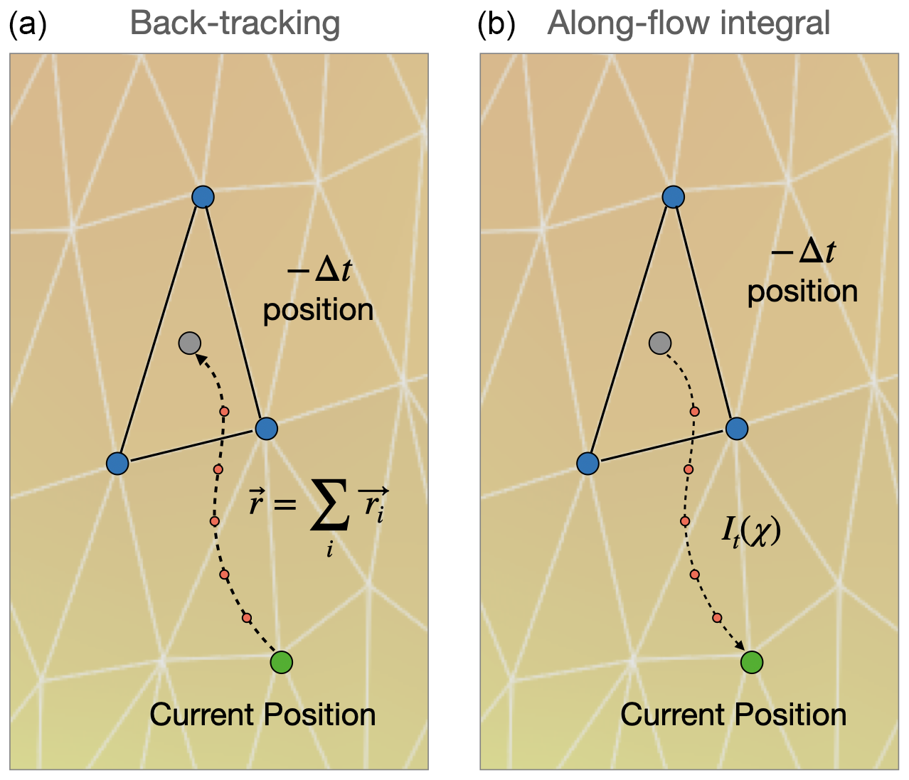
Figure 1 Schematics of a finite element mesh and a particle (here a nodal particle in green) that is back-tracked in time until reaching the position it was at previous time step (grey particle with a value interpolated from the finite element). (a) The back-tracking is divided in a series of internal time steps δt_i that can be adjusted for accuracy. (b) The source integral is then evaluated forward in time, over the same number of time steps δt_i.

A source term χ that depends on the evolution of the particle along the path integral, following a function χ(q,t), can be evaluated over time. This corresponds to solving:

$$\begin{array}{}\text{(6)}& {\displaystyle }{\displaystyle }{I}_t\left(\mathit{\chi }\right)=\underset{t-\mathrm{\Delta }t}{\overset{t}{\int }}\mathit{\chi }(q,t)\mathrm{d}t\end{array}$$

The new value of q is then reevaluated as the combination of Eqs. (5) and (6):

$$\begin{array}{}\text{(7)}& {\displaystyle }{\displaystyle }q=q({\mathit{r}}_{t-{\mathrm{\Delta }}_t},t)+I_t\left(\mathit{\chi }\right)\end{array}$$

Back-tracked particles have to be localized within the mesh at each internal time step δ_i to capture the velocity of the particle. The simplest way to find this position is to localize the particle's new location using the coordinate of the particle to retrieve its position into the mesh. The method is accurate but very inefficient for unstructured meshes, making it very greedy in terms of computation time and memory access. In-cell test algorithms have been developed to overcome this issue (e.g. Macpherson et al., 2009; Haselbacher et al., 2007; Ketefian et al., 2016). The in-cell test allows to back-track the mesh cell where the particle resides, without the need for additional searches over the entire mesh. The shape functions associated with the nodes within the element are then evaluated, and the interpolation is performed using the nodal values.

Our particle-tracking algorithm is based on the method developed by Macpherson et al. (2009). It involves tracking the motion of particles from element to element by checking whether or not an element face is crossed over an internal time step. Similarly to Macpherson et al. (2009), let's define a particle with an initial position r(t) corresponding to a node. For each internal time step δ_i of the back-tracking procedure, a check is performed to evaluate whether or not one of the faces of the element has been crossed. This is done through geometrical considerations via the calculation of determinants between the vectors formed by the initial and final locations of the particle over the internal time step on the one hand, and the vectors formed by the positions of the nodes of the considered element face on the other hand. If it turns out that a face has been crossed, the face index is used to determine which element, if any, is on the other side of the face. Then, the algorithm is continued from this new element for each remaining internal time step δ_i until the end of the main simulation time step Δ_t. While the method requires some complex geometrical tests, it is shown that computational time scales approximately linearly (𝒪(N_p)) with the number of particles (N_p), as only local operations are performed. This makes the method faster than most tree-based localizations that are shown to scale logarithmically (𝒪(N_plog N_p)). More detail on the particle location and element crossing, as well as the interaction with boundary interfaces can be found in the Appendix A.

2.2 Discontinuous Galerkin advection

In Elmer/Ice, the advection equation Eq. (1) can also be solved by applying a discontinuous Galerkin method (DG). Similarly to the SL algorithm, the flow solution does not rely on a DG formulation; only the advection equation employs a DG formulation. The implementation of the method mostly relies on the work of Brezzi et al. (2004) for solving first-order linear hyperbolic equations. In this method, the stability of the numerical scheme (i.e. the stabilization of the oscillations near the discontinuities) is ensured by adding a jump-penalty term to the discretized Eq. (1) without requiring upwind stabilization or other terms. Only a short summary is presented here.

To apply the DG method with jump-penalty stabilization to the advection equation, we begin by rewriting Eq. (1 in its weak form by multiplying it by a discontinuous test function v_h and integrating over each element T:

$$\begin{array}{}\text{(8)}& {\displaystyle }{\displaystyle }\underset{T}{\int }{\displaystyle \frac{\partial q_h}{\partial t}}{v}_h\mathrm{d}x+\underset{T}{\int }\mathit{u}\cdot \mathrm{\nabla }{q}_h{v}_h\mathrm{d}x=\underset{T}{\int }S{v}_h\mathrm{d}x.\end{array}$$

Integrating the advection term by parts, we obtain:

$$\begin{array}{}\text{(9)}& {\displaystyle }{\displaystyle }\underset{T}{\int }\mathit{u}\cdot \mathrm{\nabla }{q}_h{v}_h\mathrm{d}x=-\underset{T}{\int }{q}_h\mathit{u}\cdot \mathrm{\nabla }{v}_h\mathrm{d}x+\underset{\partial T}{\int }\mathit{u}\cdot \mathit{n}{q}_h{v}_h\mathrm{d}s,\end{array}$$

where n is the outward normal on ∂T.

The DG formulation can then be expressed as:

$$\begin{array}{ll}{\displaystyle }& {\displaystyle }\sum _{T\in {\mathcal{T}}_h}\underset{T}{\int }{\displaystyle \frac{\partial q_h}{\partial t}}{v}_h\mathrm{d}x-\sum _{T\in {\mathcal{T}}_h}\underset{T}{\int }{q}_h\mathit{u}\cdot \mathrm{\nabla }{v}_h\mathrm{d}x\\ {\displaystyle }& {\displaystyle }+\sum _{e\in {\mathcal{E}}_h}\underset{e}{\int }\mathit{\{}\mathit{u}\cdot \mathit{n}{q}_h\mathit{\}}\left[\right[v_h\left]\right]\mathrm{d}s\\ \text{(10)}& {\displaystyle }& {\displaystyle }+\sum _{e\in {\mathcal{E}}_h}\underset{e}{\int }{\mathit{\alpha }}_e\left[\right[q_h\left]\right]\left[\right[v_h\left]\right]\mathrm{d}s=\sum _{T\in {\mathcal{T}}_h}\underset{T}{\int }S{v}_h\mathrm{d}x.\end{array}$$

where the third term ${\int }_e\mathit{\{}\mathit{u}\cdot \mathit{n}{q}_h\mathit{\}}\left[\right[v_h\left]\right]\mathrm{d}s$ captures the advection across the element interface e using the average flux, with [[v_h]] being the jump operator representing the difference in v_h between the two sides of e, and {u⋅n q_h} represents the mean flux across e. The fourth term ensures stability by penalizing large jumps in q_h across element edges, where α_e is a penalty parameter, often set as ${\mathit{\alpha }}_e=\frac{|\mathit{u}\cdot \mathit{n}|}{\mathrm{2}}$. This penalization helps prevent spurious oscillations and improves the convergence of the solution.

3 Synthetic experiments

To illustrate the performance of our SL model, we have conducted two numerical experiments that solve simple transport problems. The first experiment, using the Zalesak disc (Zalesak, 1979), allows us to evaluate the ability of our model to transport sharp shapes while guaranteeing their conservation in a simple 2D framework. The second test allows us to evaluate the performance of the transport in a 3D framework. In both of these simple cases, the SL framework is evaluated against the Eulerian advection model usually used in Elmer with a discontinuous-Galerkin (DG) method.

Besides comparing the general patterns, the accuracy of the two methods will be evaluated using two metrics. The first metric assesses the spatial distribution of the advected field and consists of the normalized root mean square error (NRMSE) between a reference solution (q_ref) and the advected quantity (q_i with i=SL or DG):

$$\begin{array}{}\text{(11)}& {\displaystyle }{\displaystyle }\text{NRMSE}\left(q_i\right)={\displaystyle \frac{\mathrm{1}}{\mathrm{\Omega }}}\sqrt{{\displaystyle \frac{{\int }_{\mathrm{\Omega }}(q_{\text{ref}}-q_i{)}^{\mathrm{2}}}{max\left(q_{\text{ref}}\right)}}}\mathrm{d}\mathrm{\Omega }.\end{array}$$

The second metric is used to assess conservation, i.e. we expect the integral of the field q over the domain Ω to remain constant over time, and the following quantity to remain equal to 0 (for a closed system and without a source/sink term in Eq. 6):

$$\begin{array}{}\text{(12)}& {\displaystyle }{\displaystyle }\mathrm{\Delta }\left[q_i\right]={\displaystyle \frac{\mathrm{1}}{\mathrm{\Omega }}}\underset{{\mathrm{\Omega }}_s}{\int }{\displaystyle \frac{q_i-q_{\text{ref}}}{q_{\text{ref}}}}\mathrm{d}\mathrm{\Omega }.\end{array}$$

3.1 Solid bodies in rotation

This classical rotating-disc experiment is designed to assess the ability of the advection schemes to preserve sharp geometrical features and global mass under purely advective motion. Because the analytical solution corresponds to a rigid-body rotation, any deformation or diffusion of the discs can be directly attributed to numerical errors.

3.1.1 Experimental setup

We define a square domain ${\mathrm{\Omega }}_{\text{square}}=[\mathrm{0},\mathrm{1}]\times [\mathrm{0},\mathrm{1}]$, with linear (i.e. linear shape functions) square finite elements. We put 2D solid bodies in rotation within a 2D circular steady velocity field with an angular velocity $\mathit{\omega }=\mathrm{1}{\mathrm{s}}^{-\mathrm{1}}$. The discs are hence supposed to maintain their shape while rotating, allowing for the evaluation of the advection scheme's ability to accurately transport information. Simulations are performed at coarse ($R_{s,\mathrm{1}}=\mathrm{101}\times \mathrm{101}$ nodes) and fine resolution ($R_{s,\mathrm{2}}=\mathrm{201}\times \mathrm{201}$ nodes), and with different time steps, from ($\mathrm{\Delta }t=\frac{\mathrm{2}\mathit{\pi }}{\mathrm{30}}$ s to $\mathrm{\Delta }t=\frac{\mathrm{2}\mathit{\pi }}{\mathrm{1440}}$ s), to assess the sensitivity of the solution to both spatial and temporal resolution.

We perform three types of simulations:

1. SL transport of the discs without reinitialization of the particles, i.e. only one simulation timestep Δt=2π s. Given the stationary velocity field, particles do not require to be reinitialized at each time step. In this case, there is almost no loss of information since only one interpolation is needed over the entire simulation – only internal time steps (δ_i) are considered to improve the trajectory of the particles but the interpolation of the field to the particle position is made once at the end of the backward trajectory. As a consequence, we consider that this simulation can be used as a reference for the other methods.

2. SL transport with reinitialization at each time step (Δt<2π s). This case shows how the simulation would perform in a transient simulation with u=u(t).

3. Eulerian transport with a DG method. The method is applied in the same conditions as the SL transport to compare the results.

3.1.2 Results

The SL and Eulerian DG methods exhibit opposite sensitivities to spatial and temporal resolution (Figs. 2 and 3). With the SL method, the sharpness of the discs at the end of the solution increases with spatial resolution and decreases with temporal resolution. This is directly linked to interpolation errors: higher spatial resolution improves the interpolation accuracy, while smaller time steps increase the number of interpolations performed during the simulation. As Δt decreases, particles move only slightly within the same element and are therefore interpolated more frequently, leading to the accumulation of interpolation errors. For sufficiently small Δt (e.g. $\mathrm{\Delta }t\sim \mathrm{2}\mathit{\pi }/\mathrm{200}$ s for R_s1 and $\mathrm{\Delta }t\sim \mathrm{2}\mathit{\pi }/\mathrm{700}$ s for R_s2), this decrease in accuracy tends to stabilize (Fig. 3a). This saturation occurs because the interpolated values change very little between successive steps, and the cumulative interpolation error becomes effectively bounded.

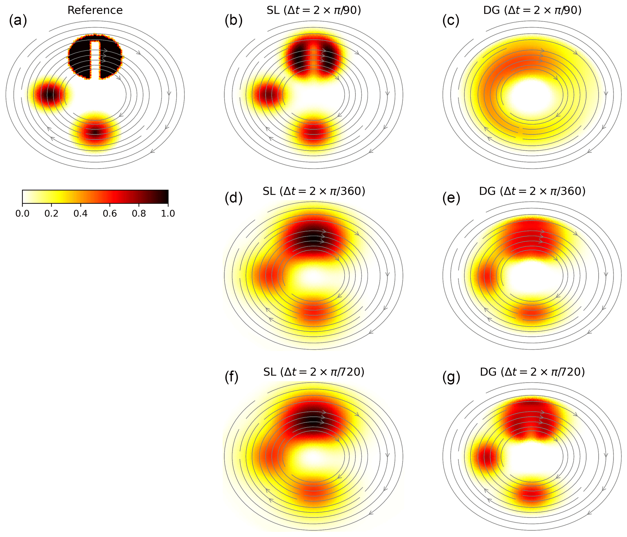
Figure 2 Evolution of two discs and one Zalesak disc after a complete rotation: (a) Reference solution (i.e. the SL solution after one rotation with no reinitialisation), (b, d, f) SL solution and (c, e, g) Eulerian DG. The simulation is conducted at the resolution R_s1 with 3 different Δt: (first line) $\mathrm{\Delta }t=\mathrm{2}\times \mathit{\pi }/\mathrm{90}$, (second line) $\mathrm{\Delta }t=\mathrm{2}\times \mathit{\pi }/\mathrm{360}$, (third line) $\mathrm{\Delta }t=\mathrm{2}\times \mathit{\pi }/\mathrm{720}$. The grey arrows show the circular direction of the flow.

Figure 3 Assessment of the SL and Eulerian DG methods after a full rotation of the three solid bodies: (a) NRMSE (Eq. 11) and (b) spatially-integrated relative bias in concentration (Eq. 12). The results are shown for low ($R_{s\mathrm{1}}=\mathrm{101}\times \mathrm{101}$ nodes) and high ($R_{s\mathrm{2}}=\mathrm{201}\times \mathrm{201}$ nodes) spatial resolutions.

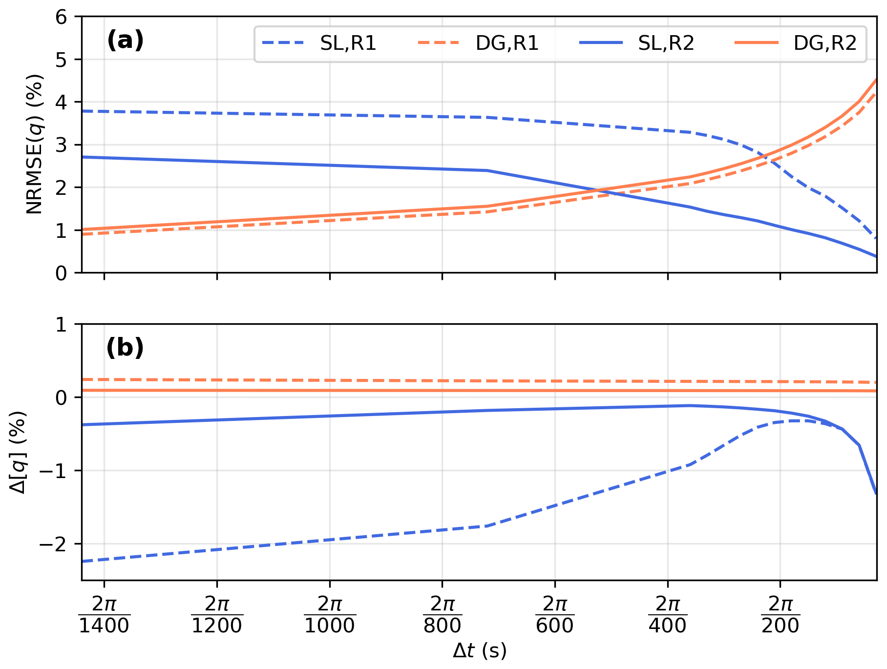
On the contrary, the accuracy of the Eulerian DG method increases mostly with temporal resolution, while showing little sensitivity to spatial resolution (Fig. 3a).

In terms of conservation, the SL method leads to a decrease of [q_i] as Δt increases, resulting in non-zero values of Eq. (12). This loss can be attributed to the non-conservative nature of the particle–mesh interpolation process, where particle values are reconstructed from nodal values using FEM shape functions. In contrast, with DG, [q_i] remains largely insensitive to changes in Δt and is therefore conservative. Finally, the diffusion introduced by the SL method is mostly isotropic, whereas the diffusion in the Eulerian DG scheme is primarily aligned with the velocity field (Fig. 2).

3.2 Tracer in a 3D slab flow

This second experiment extends the analysis to a three-dimensional setting and focuses on the influence of time stepping, parallel domain decomposition, and computational cost on tracer advection.

3.2.1 Experimental setup

This experiment involves a 3D parallelepipedal domain with a horizontal surface Ω of 100 km×50 km and a thickness of 100 m. We impose a 1000 m yr⁻¹ unidirectional flow along x. We use 3D linear hexahedral elements obtained by vertically extruding the 2D rectangular mesh into three layers and conduct the simulations at a coarse resolution (R_m,1) with 1 km×1 km elements, i.e. 15 912 nodes, and a fine resolution (R_m,2) with 250 m×250 m elements, i.e. 401 919 nodes. A donut-shaped tracer is initialized at the position x=25 km and y=25 km (center of the donut) to test the advection algorithms. The simulations are conducted for 50 years with a stationary flow. The horizontal velocities are set up so that the center of the tracer flows from x=25 km to x=75 km over the course of the simulation.

With the increasing availability of high-performance computing systems, most numerical simulations are now executed in parallel. Such parallelization can be challenging for the SL algorithm when one particle moves from one partition to another. We perform the simulations using distributed-memory parallelization with MPI only; no shared-memory (OpenMP) parallelism is employed. Inter-partition communication is carried out after each internal time step of the particle tracking to ensure consistent particle ownership across sub-domain boundaries. A dedicated scalability analysis is presented in Appendix A4. In addition, we compare the computation time of the SL and the DG methods, as well as the impact of the number N of internal time steps δ_i in Eq. (3).

3.2.2 Results

In this experiment, the SL method shows again a large sensitivity to the time-stepping choice. Given that the grid is regular and the flow velocity is uniform, steady, and unidirectional, the best results are obtained when fixing $\mathrm{\Delta }t=m\times \mathrm{\Delta }x/v_x$ (with m∈ℕ), which allows a perfect node-to-node displacement at each Δt and no interpolation requirement in the absence of any source/sink term. Once we fall into values of $\mathrm{\Delta }t<\mathrm{\Delta }x/v_x$, we rapidly see a decrease in solution sharpness with increasing diffusion as Δt decreases (Fig. 4a). Since the particles follow a straight line, there is no need for internal time steps to improve the accuracy of the trajectory and we see little to no impact of the number of internal time steps N in Eq. (3). Contrary to the previous case, where the solid shapes were moving along both x and y axes, the uni-directional trajectory only leads to interpolation error along x, allowing to have no diffusion along y, i.e. perpendicularly to the flow.

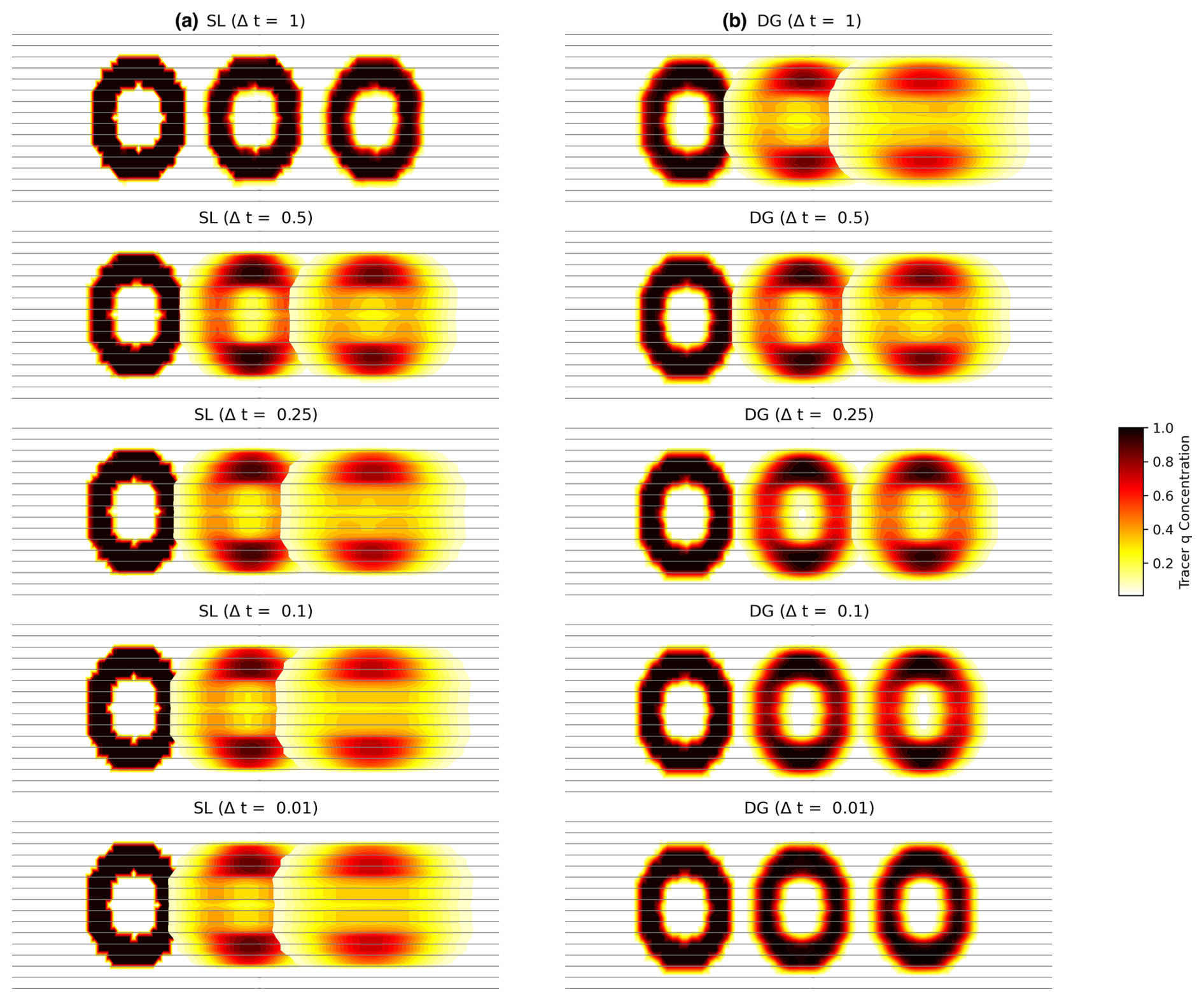
Figure 4 Donut transport with the (a) SL method (with N=5) and (b) the DG method, at 1 km resolution. The donut advects from left to right and is plotted on each panel at t=0 yr, t=25 yr, and t=50 yr. Flowlines are represented in grey.

These results stand again in opposition with the DG method which leads to better performance when using a smaller Δt (Fig. 4b), with little impact of the spatial resolution. Focusing on the calculation of the NRMSE (Eq. 11), the SL method yields smaller NRMSE as Δt increases, while the DG method leads to higher NRMSE (Fig. 5). In both cases, the rate of the NRMSE evolution decreases over time, which can be due to an increasing numerical accuracy as the solution gets smoother. In terms of concentration, the DG method leads to almost no average concentration loss (i.e. less than 1 % after 50 years) while the SL concentration oscillates up to ±4 %. This reflects the non-conservative nature of the particle–mesh interpolation: depending on the local configuration, the reconstructed field can introduce either a slight artificial gain or loss when integrated over the domain. The small oscillations visible in Fig. 5 primarily originate from the repeated reinitializations and interpolations of particle values at each simulation time step (Δt), which leads to the accumulation of rounding and interpolation errors. The number of internal sub-steps (δt, kept constant here) affects these oscillations only indirectly through its influence on trajectory accuracy. In parallel runs, additional minor deviations may arise from transient particle losses when particles cross sub-domain boundaries between MPI synchronizations; these events are rare and decrease as synchronization frequency increases.

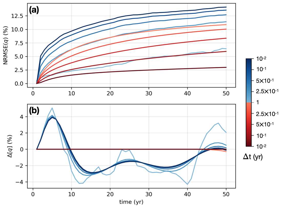
Figure 5 (a) NRMSE and (b) spatially-integrated relative bias in concentration of the donut tracer over time for different time step lengths at 1 km resolution (SL: blue shades; DG: red shades).

The computation time also differs between the methods. For identical (Δt,Δx), the computing time of the SL method increases with the number of internal time steps N (see Table 1). This behavior is approximately linear, as interpolation and mesh-related operations are performed once per simulation time step, whereas the particle advection cost scales with N. Although large values of N are not required in the present configuration, they increase the SL runtime relative to the DG method, whose cost typically falls within the range of the SL solver for N=3. Nevertheless, for the configurations considered here, these advection costs remain small compared with the computational expense of the 3D flow solvers (e.g. Stokes flow) typically used in Elmer.

Table 1 Average time (in seconds) spent in the solver over one simulation time step (Δt) for different algorithms for the 3D-slab-flow case of Sect. 3.2 for an 8-partition domain and a 1 km resolution.

4 Application of semi-Lagrangian and discontinuous Galerkin advection to ice-damage evolution in Antarctica

The experiments conducted to assess the performance of the SL method in comparison with the DG method provide valuable insights into the behavior of these numerical schemes under different conditions. These results demonstrate the trade-offs involved in using SL and DG methods, particularly in terms of accuracy, computational efficiency, and sensitivity to spatial and temporal resolutions.

Hereafter, we apply both advection schemes to a high-resolution ice sheet model to simulate the evolution of ice damage in the Amundsen Sea region, where a rapid and significant ice-sheet mass loss has been observed over the last decades (e.g. Smith et al., 2020). This rapid mass loss has led to structural changes in the ice sheet and increased damage in key areas such as shear margins (Sun and Gudmundsson, 2023; Lhermitte et al., 2020; Alley et al., 2019). These damaged areas correspond to highly crevassed regions that often appear where the ice becomes afloat and evolve as they are advected downstream over the ocean.

4.1 Numerical ice sheet setup and experiment

We build a 3D model of the region and simulate the ice flow using the state-of-the-art Stokes flow model Elmer/Ice (see Appendix B1), following the initialization procedure described in Appendix B2. The model is discretized on an unstructured finite-element mesh using stabilized equal-order linear wedge elements for velocity and pressure. Numerical integration is performed using 44 Gauss points per element (11 points on the triangular face and 4 along the vertical direction). Although the velocity and pressure are approximated with first-order Lagrange elements, this relatively high quadrature order is required to accurately integrate the nonlinear viscosity and stabilization terms within each element. Stresses are computed at these integration points and subsequently interpolated to the mesh nodes, where the damage variable is evaluated. Once initialized, we simulate the evolution of damage over 50 years.

Our damage model is based on Continuous Damage Mechanics (CDM) and follows the same physical approach as Krug et al. (2014) and Gilbert et al. (2015): damage is created where the maximum tensile principal stress exceeds a threshold and is advected downstream with the flow. The corresponding advection equation with a source term is solved using either the SL or the DG solver described previously.

To keep the case as simple as possible, we use a constant source term for damage and focus only on the creation of surface damage (i.e. we do not include basal damage due to water pressure in Eq. B11). We also ignore feedbacks between damage and viscosity (see Eq. B6). Details of the damage model are presented in Appendix B3. A key parameter of the model is the stress threshold σ_th at which damage occurs. In previous studies, σ_th is often taken between 0.1–0.3 MPa (e.g. Krug et al., 2014; Albrecht and Levermann, 2012; Grinsted et al., 2024). Here, we select a particularly high value of σ_th=0.55 MPa to limit damage production (χ>0) to areas clearly identified as crevasse onset regions in observations (Lhermitte et al., 2020). Additionally, mountainous regions and steep slopes are excluded from the simulations as these areas are unlikely to sustain ice cover.

Our synthetic experiments indicated that using longer SL advection time steps (Δt) combined with multiple internal time steps (δ_i) helps limit the interpolation errors that accumulate over repeated advection cycles. This issue is particularly acute in high-resolution ice-flow models (e.g. Δx∼1 km), where small time steps (e.g. $\mathrm{\Delta }t\sim {\mathrm{10}}^{-\mathrm{2}}$ year) are typically required for the flow solver to limit feedbacks between vertical velocities and free-surface evolution.

To address this, the SL advection step is executed with a larger time step than the flow solver (Δt>Δt_flow), reducing both interpolation frequency and computational cost. Because feedbacks between damage and viscosity are disabled in this experiment, this reduced update frequency does not affect the flow solution. In a fully coupled setup, such decoupling would introduce a trade-off between numerical diffusion and the accuracy of damage-flow interactions. However, as our focus is solely on evaluating numerical diffusion, deactivating the feedback allows us to better compare stepping choices.

We conduct a set of eight simulations of damage evolution using the same steady-state geometry, ice flow, and damage model parameters. Each simulation covers 50 years of damage evolution with SL advection time steps ranging from $\mathrm{\Delta }t={\mathrm{10}}^{-\mathrm{2}}$ to 5 year. The same simulations are performed using the DG advection scheme for comparison.

4.2 Damage simulation results

The simulations reproduce the main damage structures observed in the Amundsen Sea sector, with damage primarily generated in shear margins near the grounding line of Pine Island Glacier and subsequently advected downstream along flowlines that follow patterns observed in satellite imagery (e.g. Lhermitte et al., 2020). Over the Thwaites Ice Shelf, damage is more widespread but still aligns with the general patterns inferred from observations. Both advection schemes capture the large-scale transport of damage from upstream source regions toward the ice shelves.

In a purely advective setting without numerical diffusion, damage generated in localized source regions should remain laterally confined to the downstream flowlines along which it originates. To visualize potential spreading caused by numerical diffusion, we overlay flowlines with spacing ranging from about one to three elements (approximately 500 m to 5 km depending on the region).

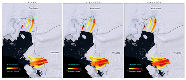
For the SL simulations, decreasing the advection time step Δt–and therefore increasing the number of particle–mesh interpolation operations–leads to increased smoothing of the vertically integrated damage field, producing progressively smoother damage patterns (Fig. 6). This effect is particularly noticeable over Thwaites Glacier and its ice shelf, where margins and sharp structures become increasingly diffuse as Δt decreases. For instance, for Δt=1 yr (Fig. 6a), only limited lateral spreading is observed: damage generated upstream remains largely confined within one flowline spacing ($D_{\text{mean}}<{\mathrm{10}}^{-\mathrm{3}}$). Smaller time steps of $\mathrm{\Delta }t={\mathrm{10}}^{-\mathrm{1}}$ yr (Fig. 6b) and $\mathrm{\Delta }t={\mathrm{10}}^{-\mathrm{2}}$ yr (Fig. 6c) lead to progressively stronger lateral spreading, with damage originating from neighboring ice streams occasionally merging downstream. In addition, we observe cumulative smoothing and a gradual loss of damage intensity along the flowlines as the signal is advected farther from its source, an effect that is particularly visible along the shear margins of Pine Island Glacier and consistent with the non-conservative nature of the particle–mesh remapping.

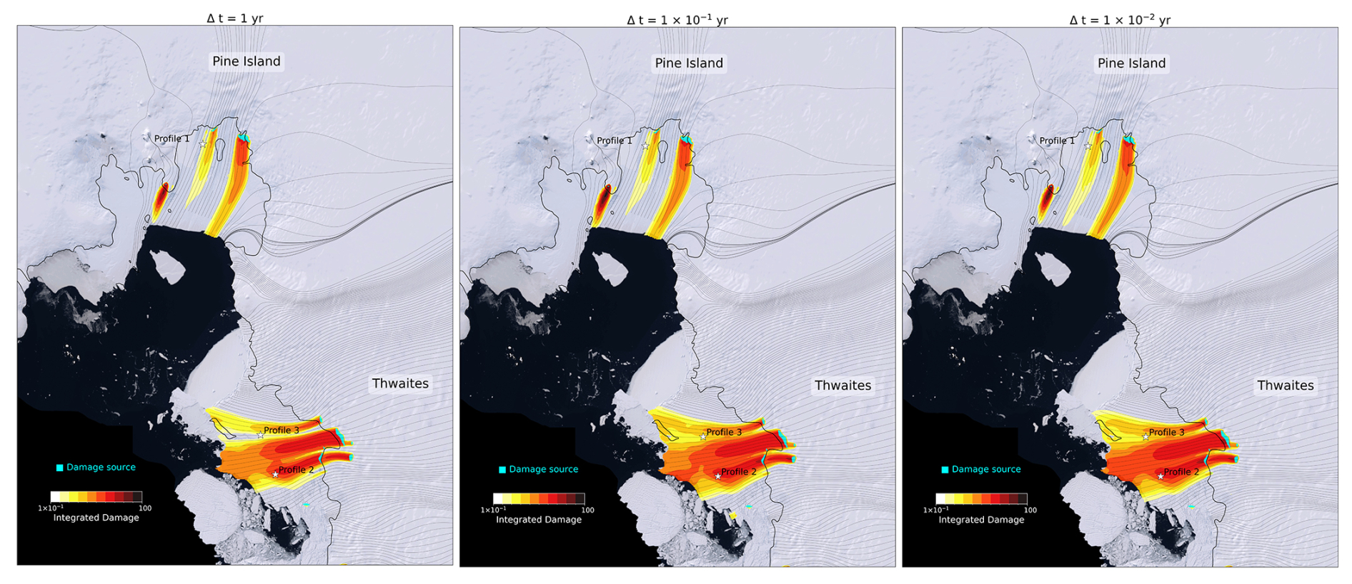
Figure 6 Semi-Lagrangian (SL) vertically integrated damage after 50 years of simulation in the Amundsen Sea Sector for different time steps: (a) Δt=1 yr, (b) $\mathrm{\Delta }t={\mathrm{10}}^{-\mathrm{1}}$ yr, and (c) $\mathrm{\Delta }t={\mathrm{10}}^{-\mathrm{2}}$ yr. All the simulations were conducted with a σ_th=0.55 MPa, and no damage retro-action neither on the viscosity nor on the damage source term, i.e. D=0 in Eqs. (B6) and (B11). The grounding line is represented with a thick black line, the flowlines with thin grey lines, and the sources for damage are represented in cyan. The Landsat Image Mosaic of Antarctica (LIMA) for the region is plotted in background. The location of Pine Island and Thwaites glacier is indicated for reference.

The DG simulations exhibit a different spreading structure. While the large-scale damage patterns remain comparable, diffusion occurs preferentially along the flow direction. As a result, damage features tend to extend farther downstream from the source regions for larger time steps, producing elongated streaks aligned with the velocity field. This contrasts with the SL solution, where smoothing arises primarily from particle–mesh interpolation and therefore appears more isotropic, with only a secondary influence from mesh orientation. At the same time, the DG formulation preserves tracer intensity more effectively, reflecting its locally conservative nature. These differences are consistent with the behavior observed in the synthetic benchmark experiments. Small oscillatory patterns can also be observed along some DG damage trajectories, appearing as triangular structures aligned with the mesh elements. These features likely reflect element-wise reconstruction and limiting operations used in the DG discretization. Although these mesh-scale artefacts remain localized and do not significantly affect the large-scale damage distribution, they highlight differences in how the two schemes handle steep tracer gradients during advection.

We can also assess numerical diffusion by examining three vertical damage profiles at different locations (see locations in Fig. 6 and profiles in Fig. 8). On Profile 1 (Fig. 8)a, d), located within a shear margin of Pine Island Glacier and downstream of a damage source, the overall damage distribution remains relatively similar for both advection schemes. However, for the SL simulations, decreasing Δt leads to a reduction in the maximum damage near the surface. The DG simulations show the opposite tendency, with the surface maximum decreasing as Δt increases. We also observe a deeper penetration of damage into the ice column as Δt decreases or increases, depending on the method but this effect is stronger with SL. One exception occurs for very large SL time steps (e.g. Δt=5 yr), which produce slightly lower damage within the upper ∼100 m of the ice column. This behavior may result from reduced numerical diffusion of damage originating from adjacent flowlines. Profile 2, located downstream of a damage source of Thwaites Glacier, exhibits a similar pattern (Fig. 8b and e). Conversely, Profile 3 which is situated between two damage sources and is not downstream of any specific source, exhibits low to no damage for Δt=5 yr SL simulation. In the absence of numerical diffusion, the ice should remain undamaged at this location. However, due to numerical diffusion, damage appears and increases rapidly as Δt decreases for the SL, before stabilizing once the particle displacement per time step becomes small enough that further interpolations have a lesser impact on the results (Fig. 8c). The DG simulations also show the effect of numerical diffusion but to a lesser extent. Overall, the vertical profiles for both methods tend to converge toward similar damage distributions as Δt decreases for SL and increases for DG, suggesting that numerical diffusion approaches a plateau for both schemes

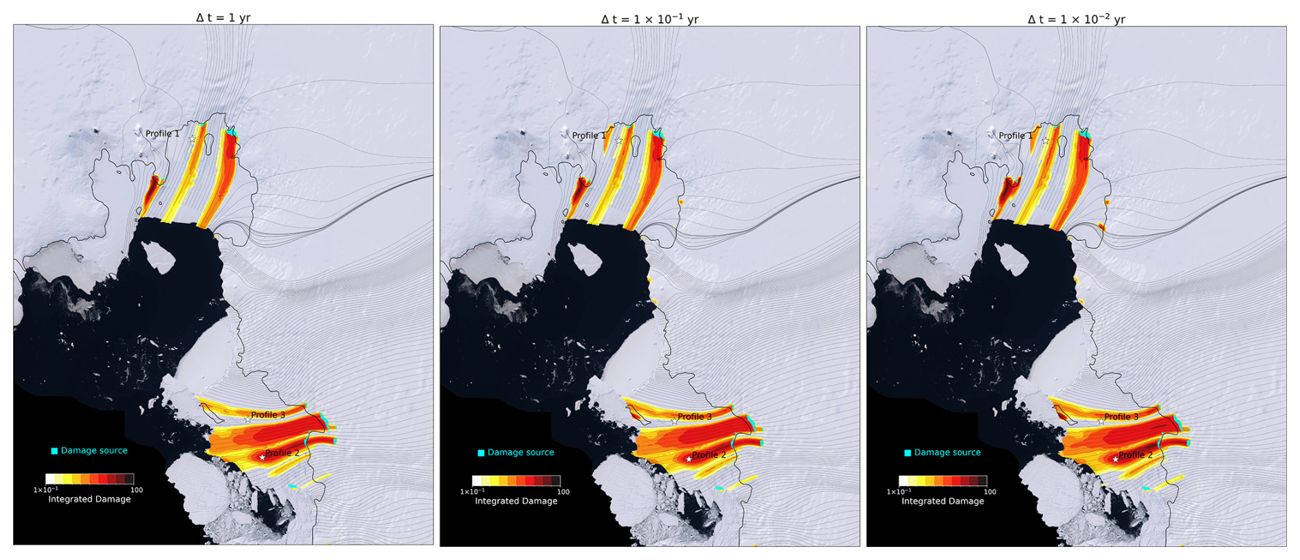
Figure 7 Same as Fig. 6 but with the Discontinuous Galerkin (DG) solver. The Landsat Image Mosaic of Antarctica (LIMA) for the region is plotted in background.

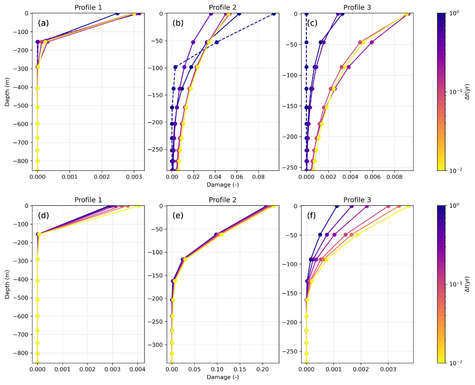
Figure 8 Vertical damage profiles after 50 years of simulation for three locations shown in Figs. 6 and 7. Panels (a–c) correspond to the semi-Lagrangian (SL) solver and panels (d–f) to the Discontinuous Galerkin (DG) solver. The three columns show results for (a, d) Profile 1, (b, e) Profile 2 (b, e), and (c, f) Profile 3. Colored solid lines indicate the different advection time steps Δt, while the dashed line indicates the case Δt=5 yr.

In addition to the differences in numerical diffusion, the two advection schemes exhibit markedly different computational costs in the present configuration. In the Antarctic experiments, the DG simulations require an advection time step of order $\mathrm{\Delta }t\approx {\mathrm{10}}^{-\mathrm{2}}$ yr. In contrast, accurate SL solutions are obtained with Δt=1 yr using N=10 internal timesteps for trajectory integration. Under these conditions, the SL advection step is roughly ∼50–100 times cheaper than the DG solver at the same mesh resolution. While the SL still shows diffusion at Δt=1 yr, this computing time difference could allow for the SL solver to run with ∼50–100 times more particles for a similar cost as the DG solver at $\mathrm{\Delta }t\approx {\mathrm{10}}^{-\mathrm{2}}$ yr.

5 Discussion and future adaptations

The current application of the SL method to damage evolution in the Amundsen Sea sector of Antarctica provides a practical demonstration of both the challenges and benefits of the method in glaciological simulations. The SL method's sensitivity to time step length directly impacts the diffusion of the damage field: longer time steps reduce numerical diffusion. The observed lateral diffusion of damage along flowlines, especially in regions like Thwaites Glacier, underscores the importance of carefully selecting time step parameters to minimize unwanted diffusion while ensuring computational feasibility. While small time steps are typically required for solving ice flow (i.e. Stokes flow in our case) and free-surface evolution (usually about $\mathrm{\Delta }t={\mathrm{10}}^{-\mathrm{2}}$ yr), we have proposed to address the issue by decoupling the time stepping of damage evolution from the rest of the simulation. However, this approach may compromise the accuracy of the coupling between ice flow and damage evolution, which could pose challenges in capturing short timescale dynamics, such as sub-annual variations in ice flow and damage. More generally, this highlights that DG and SL schemes exhibit complementary numerical behaviors that are controlled by different error mechanisms. DG primarily benefits from time-step refinement, whereas the SL accuracy is largely controlled by spatial resolution and, critically, by the number of interpolation operations: fewer (but larger) advection steps reduce the accumulation of interpolation-driven diffusion. This distinction is important in coupled applications, where frequent exchanges between the flow solver and the transport step can amplify interpolation errors and provide the motivation for testing reduced coupling frequencies in Sect. 4.

Another practical advantage of the SL formulation is its ability to advect multiple fields within a single solver execution. This feature makes the method particularly attractive for problems involving several passively advected quantities, such as tracers, since particle trajectories can be computed once and reused for all transported variables. When source or sink terms are present, only the trajectories can be shared, while the source and sink contributions must still be evaluated separately for each field. Nevertheless, this strategy can substantially reduce the computational cost compared to Eulerian approaches, which typically require solving the full advection equation independently for each transported variable.

We outline four strategies to further improve the accuracy of the SL method in Elmer and potentially increase the coupling frequency between Stokes flow and SL damage advection, without introducing additional numerical diffusion:

• Since the additional computing cost of the SL method is usually relatively cheap to run with respect to the Stokes flow (or any flow) simulation, one possible improvement would be to run the SL method on a higher-resolution mesh than the rest of the simulation. In this approach, the Stokes flow would be computed on a coarser base mesh, and the resulting velocity field and SL source term would be interpolated onto the finer mesh for the advection step. At each time step, the advected field – such as damage – would be updated on the fine mesh and then reinterpolated back onto the coarse mesh to compute a new viscosity and solve the Stokes problem again. The velocity field will remain unchanged across both meshes but the finer resolution and the increased number of particles will improve the interpolation of the advected fields.

• Another solution would consist in dynamically adjusting the mesh during the simulation, enabling local refinement in regions of strong gradients and thereby reducing interpolation errors. Adaptive mesh refinement strategies have been shown to improve the representation of sharp advective features by locally increasing resolution (Wirbel et al., 2018). Remeshing tools such as Dapogny et al. (2014) are already interfaced with Elmer but their impact in the present context still needs to be quantified, in particular with respect to the trade-off between accuracy gains, additional computational cost, and potential interpolation errors introduced by the remeshing procedure itself.

• Instead of increasing the resolution, the SL particles could be initialized at Gauss points used for the integration of the flow problem, which number can be larger than the number of nodes (Ouardghi et al., 2022, e.g.). For example, in Elmer, we typically employ up to 44 Gauss integration points when solving the Stokes equations on linear triangular wedge elements, which could considerably increase the number of particles and the accuracy of trajectories and interpolation. However, this solution requires additional development to our current implementation of the SL problem in Elmer.

• Increasing the spatial resolution of the model can reduce spatially integrated bias in the concentration of the solution, as demonstrated in our first experiment. However, a more robust solution would be to develop a conservative formulation for the particle–mesh remapping, which is not currently implemented in Elmer. The synthetic tracer experiments indicate that the dominant limitation of the present SL implementation is not the accuracy of the trajectory integration itself, but the repeated interpolation used to reconstruct the advected field on the Eulerian mesh. Because this remapping is not strictly conservative, it introduces cumulative smoothing and a gradual loss of tracer intensity over time. Conservative SL approaches enforce tracer conservation during the remapping step by redistributing tracer mass across the computational mesh, and would likely improve amplitude preservation in the present framework. However, conservative remapping schemes can also introduce shape distortions or numerical oscillations due to the inherent difficulty of simultaneously preserving conservation and monotonicity (e.g. Priestley, 1993).

Taken together, the experiments indicate that the main limitation of the present SL implementation lies in the non-conservative particle–mesh remapping used to reconstruct the advected field. While the DG formulation better preserves tracer intensity, it introduces diffusion preferentially aligned with the flow direction and remains, to some extent constrained by smaller timesteps.

Developing conservative remapping strategies that better preserve tracer amplitude while maintaining the flexibility of the SL approach, therefore, represents an important direction for future developments in Elmer.

Finally, particle–grid approaches such as Particle-in-Cell (PiC) or Markers-in-Cell, introduced in Sect. 1, could provide an alternative strategy for tracer advection. In these methods, particles are advected forward in time while carrying tracer properties, and their values are periodically projected back onto the Eulerian mesh using conservative weighting, which can improve mass conservation and represent sub-grid variability. However, such schemes typically require maintaining a large number of particles per element to ensure adequate sampling, and particle–mesh communication as well as particle repopulation can become costly on unstructured meshes. While implementing an efficient PiC framework in Elmer would require substantial modifications to the current FEM-based data structures, they represent a promising avenue for the future evolution of Elmer particle-based implementations.

6 Conclusions

In this study, we implemented a semi-Lagrangian (SL) advection scheme in the finite-element ice-flow model Elmer/Ice (v26.1) and evaluated its performance for the transport of ice-damage fields. The SL formulation was benchmarked against a discontinuous Galerkin (DG) advection scheme through idealized tests and applied to a realistic Antarctic configuration to assess its behavior in a glaciological context. The results highlight the distinct numerical characteristics of the two approaches: the SL method enables the use of larger time steps with competitive accuracy but introduces numerical diffusion associated with repeated particle–mesh interpolation, whereas the DG scheme provides sharper transport of damage gradients at the cost of stricter time-step constraints. The Antarctic application demonstrates that both approaches can be used to simulate the large-scale evolution of ice damage, while illustrating the trade-offs between computational efficiency and numerical diffusion when modeling damage transport in ice-sheet simulations.

The DG method is particularly effective in scenarios requiring high temporal precision, as it shows significant accuracy improvements with smaller time steps. This makes DG suitable for rapidly evolving flows. On the other hand, the SL method benefits from increasing the time step size and spatial resolution, performing best when the time step allows particles to move precisely from node to node. This characteristic makes the SL method advantageous in relatively steady flows where the time step at which the transport equation is solved can be decoupled from the time step at which the velocity field is recomputed.

In recent years, research on ice sheet and glacier evolution has highlighted the importance of damage processes, but without thoroughly addressing the limitations of current advection methods regarding numerical stability, potential artifacts, or excessive diffusion (e.g. Sun et al., 2017; Lhermitte et al., 2020; Ranganathan et al., 2025; Li et al., 2025). The application of the SL method to ice damage evolution in the Amundsen Sea sector yields promising results, suggesting that Elmer/Ice simulations could effectively incorporate ice damage–a critical factor for accurate predictions of ice sheet and glacier evolution. Although the present simulations are steady in order to facilitate the characterization of numerical diffusion, the formulation of the SL advection scheme does not introduce mechanisms that would inherently lead to convergence or stability issues in transient simulations.

Looking ahead, the SL method's potential is likely to grow with advancements in computing power, which will enable finer spatial resolutions but also longer stable time steps of the free-surface problem in ice-flow and ice-sheet simulations (e.g. Löfgren et al., 2022).

For now, Elmer allows the SL method to be run at a lower frequency than the flow model itself, reducing diffusion at the expense of physical precision. As computing capabilities advance, we expect the SL method to become an even more powerful tool in glaciological simulations.

Appendix A: Semi-Lagrangian Model

A1 Implementation improvements to the semi-Lagrangian solver in Elmer/Ice

The SL solver used in this study has existed in the Elmer framework for many years. However, several limitations in the original implementation made it unsuitable for the advection of active tracers such as the damage variable considered here. In particular, the previous formulation did not properly handle source terms that depend explicitly on the transported variable. As part of the present work, several improvements and corrections have been implemented and validated. These include:

• Correct treatment of source terms that explicitly depend on the advected variable.

• Improvement of the path-integral formulation by allowing forward integration of the source term along the particle trajectory, as illustrated schematically in Fig. 1.

• Improved handling of initial conditions, enabling reliable restart capabilities for long simulations.

• Improved treatment of boundary conditions to avoid undesired particle loss near domain boundaries.

• Corrections and improvements related to parallel execution and MPI communication.

These developments were implemented primarily in the modules ParticleUtils.F90 and ParticleAdvector.F90. The evolution of these implementations is documented in the Elmer GitHub repository. The improvements were validated through extensive testing in both idealized benchmark experiments and realistic glaciological simulations.

A2 Particle location and element crossing

The first part of the motion (in the starting element and until reaching the element face at a location p) can be found using:

$$\begin{array}{}\text{(A1)}& {\displaystyle }{\displaystyle }\mathit{p}=\mathit{r}\left(t\right)+\mathit{\lambda }\left(\mathit{r}\right(t-\mathit{\delta }t)-\mathit{r}(t\left)\right)\end{array}$$

where λ is the fraction along the line $\mathit{r}(t-\mathit{\delta }t)-\mathit{r}\left(t\right)$ where the interaction occurs with the element face.

In the case of a 2D plan tracking, we can define I as the point corresponding to the initial position (i.e. at t) of the particle, F as the point corresponding to the final position (i.e. at t−δt) of the particle, and A and B as the positions of the two nodes forming the tested face (or segment in this 2D case; Fig. A1).

Let's define two vectors, IF and AB. If $\mathit{I}\mathit{F}\times \mathit{A}\mathit{B}=\mathrm{0}$, this indicates that IF and AB are parallel, and therefore, no intersection exists between the lines they define.

Next, we compute $\frac{\mathit{I}\mathit{F}\times \mathit{I}\mathit{A}}{\mathit{I}\mathit{F}\times \mathit{A}\mathit{B}}$. If this ratio is negative or greater than 1, it indicates that the line defined by IF intersects the line defined by AB outside the segment AB. As a result, there is no intersection between the particle path and the segment AB.

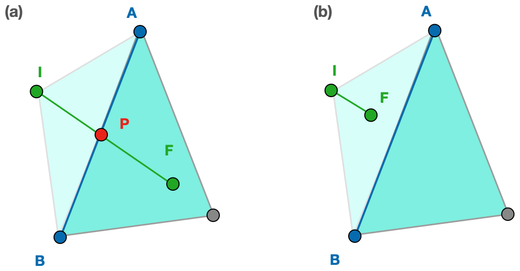
Figure A1 Representation of a trajectory (IF) from an initial point (I, here at a node of a triangular element) to a final point F in another element. (a) The segment IF intersects the face segment AB at point P. (b) The segment IF is too short to intersect the face segment AB.

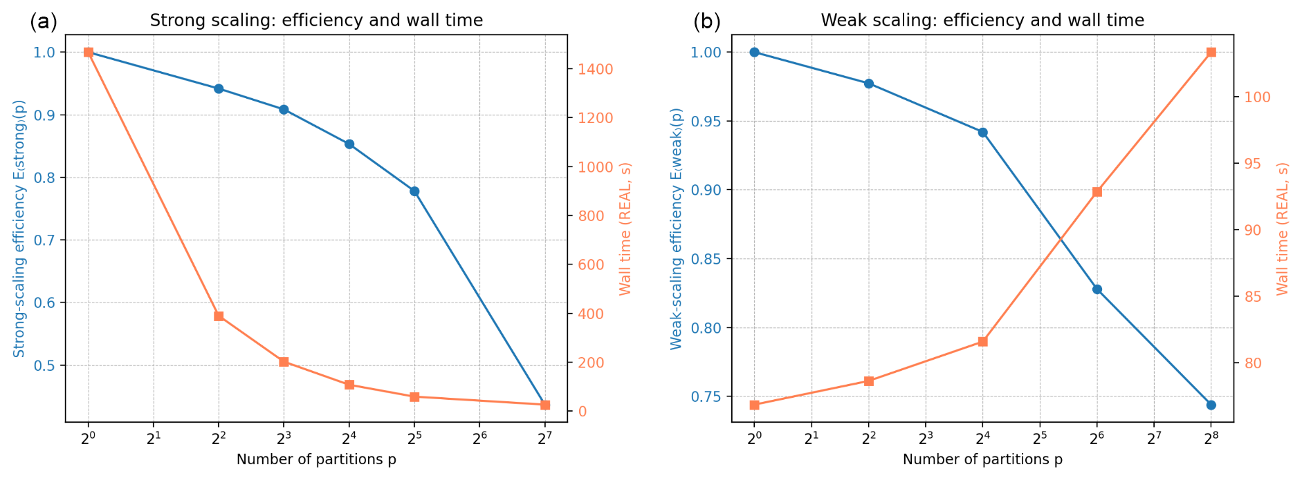
Figure A2 Parallel scalability of the semi-Lagrangian solver. (a) Strong scaling efficiency and wall-clock time as a function of the number of partitions p, obtained by increasing the number of processors while keeping the total problem size constant. (b) Weak scaling efficiency and wall-clock time as a function of p, where the workload per partition is kept constant. Efficiency is defined relative to the single-partition reference case, and wall time corresponds to the elapsed time for 100 simulation time steps to reduce variability.

Finally, we calculate λ following

$$\begin{array}{}\text{(A2)}& {\displaystyle }{\displaystyle }\mathit{\lambda }={\displaystyle \frac{\mathit{I}\mathit{A}\times \mathit{A}\mathit{B}}{\mathit{I}\mathit{F}\times \mathit{A}\mathit{B}}}.\end{array}$$

If λ>1, the segment IF is too short to intersect AB. If λ<0, there is also no intersection (point I is on the opposite side of AB). If λ<1, an intersection occurs, where

$$\begin{array}{}\text{(A3)}& {\displaystyle }{\displaystyle }\mathit{\lambda }={\displaystyle \frac{IP}{IF}},\end{array}$$

with P representing the intersection point of lines IF and AB.

A3 Boundary interactions and parallelization

At every face crossing, a check is performed to determine whether the face corresponds to a domain boundary or is an interface between two elements of the mesh. In case of parallel computing, the element face crossed can also stand at the interface between two mesh partitions. Specific actions can be undertaken depending on the type of boundary encountered:

• partition boundary: the particle position is moved to the other partition and the tracking continues in this partition.

• physical boundary: the particle is back-tracked outside the mesh. This can happen when the velocity vector points outward across the domain boundary, i.e. is not tangent to the boundary. In such case, two options are possible: (1) the particle tracking can be stopped at the boundary, effectively treating it as a solid wall; or (2) the particle can be allowed to continue its trajectory along a path tangent to the boundary surface. The same occurs for the forward tracking of the source term.

A4 Scalability Analysis

Scaling tests were conducted on the 3D slab flow experiment with the SL method (Sect. 3.2). Strong-scaling tests were performed by fixing the global problem size while increasing the number of MPI partitions from 1 to 256. Weak-scaling tests were conducted by increasing the global problem size proportionally to the number of partitions while keeping the number of mesh nodes and particles per partition approximately constant (with less than 1 % variation in the number of nodes per partition). All experiments were executed using distributed-memory MPI parallelization only on a high-performance computing system equipped with dual AMD EPYC Rome processors (128 cores per node) and 228 GB of RAM per node (approximately 1.8 GB per core).

Strong-scaling efficiency remains above 0.8 up to 16 partitions and decreases to approximately 43 % at 128 partitions, reflecting the growing impact of communication and synchronization costs relative to computation. The solver exhibits good weak-scaling behavior up to 64 partitions, with efficiencies above 80 %. At larger partition counts, efficiency decreases gradually due to increased inter-partition particle exchanges and MPI communication overhead. Nevertheless, the corresponding wall-clock time increase remains moderate, indicating acceptable scalability for large three-dimensional applications.

Appendix B: Mechanical Models

B1 Ice flow model

For continuously deforming fluids, the equation of state can be written as:

$$\begin{array}{}\text{(B1)}& {\displaystyle }{\displaystyle }\mathrm{\nabla }\cdot \mathit{\sigma }+{\mathit{\rho }}_i\mathit{g}=\mathrm{0},\end{array}$$

where ∇⋅ is the divergence operator, g is gravity, and $\mathit{\sigma }=\mathit{\tau }-p\mathbf{\text{I}}$ is the Cauchy stress tensor, which links the deviatoric stress tensor τ and the isotropic pressure p, where I is the identity matrix. Stress can then be linked to strain rate with an isotropic power law known as Glen's flow law (Glen, 1955), written as

$$\begin{array}{}\text{(B2)}& {\displaystyle }{\displaystyle }\mathit{\tau }=\mathrm{2}\mathit{\eta }\dot{\mathit{\epsilon }},\end{array}$$

where η is the effective viscosity, and $\dot{\mathit{\epsilon }}$ is the strain-rate tensor, defined as

$$\begin{array}{}\text{(B3)}& {\displaystyle }{\displaystyle }{\dot{\mathit{\epsilon }}}_{ij}\equiv {\displaystyle \frac{\mathrm{1}}{\mathrm{2}}}\left({\displaystyle \frac{\partial u_i}{\partial x_j}}+{\displaystyle \frac{\partial u_j}{\partial x_i}}\right).\end{array}$$

with u_i the components of the velocity vector u. The effective viscosity, η, in Eq. (B2) is given by:

$$\begin{array}{}\text{(B4)}& {\displaystyle }{\displaystyle }\mathit{\eta }={\displaystyle \frac{\mathrm{1}}{\mathrm{2}}}(E_{\mathrm{D}}A{)}^{-\mathrm{1}/n}{{\mathit{I}}_{\dot{\mathit{\epsilon }}}}_{\mathrm{2}}^{(\mathrm{1}-n)/n},\end{array}$$

where E_D is an enhancement factor, ${{\mathit{I}}_{\dot{\mathit{\epsilon }}}}_{\mathrm{2}}=\sqrt{{\dot{\mathit{\epsilon }}}_{ij}{\dot{\mathit{\epsilon }}}_{ij}/\mathrm{2}}$ is the second invariant of the strain-rate tensor and n is the Glen exponent, with an empirically determined value between 1–5 (Weertman, 1983; Gillet-Chaulet et al., 2011). An average value of n=3 is usually used in ice sheet models and is also applied in this study. A is the fluidity, which depends on the temperature following Arrhenius' law:

$$\begin{array}{}\text{(B5)}& {\displaystyle }{\displaystyle }A=A_{\mathrm{0}}{\mathrm{e}}^{-Q/\left(RT\right)},\end{array}$$

with A₀ a reference fluidity or prefactor, Q the activation energy, R the gas constant, and T the temperature (units of K). Following Cuffey and Paterson (2010), we set the reference fluidity to $A_{\mathrm{0}}=\mathrm{1.258}\times {\mathrm{10}}^{\mathrm{13}}$ ${\mathrm{MPa}}^{-\mathrm{3}}{\mathrm{a}}^{-\mathrm{1}}$ and the activation energy to Q=60 kJ mol⁻¹ for T<263 (K−10°C), and $A_{\mathrm{0}}=\mathrm{6.046}\times {\mathrm{10}}^{\mathrm{28}}$ ${\mathrm{MPa}}^{-\mathrm{3}}{\mathrm{a}}^{-\mathrm{1}}$ and Q=139 kJ mol⁻¹ for T>263 K. The code is based on a 3D Finite Element Method (FEM) for numerically solving the Stokes equations, computing ice flow by solving Eq. (B1) subject to the principle of mass conservation, $\mathbf{\nabla }\cdot \mathit{u}=\mathrm{0}$.

In the context of continuum mechanics, fractures and crevasses that weaken the ice can be represented by reducing the enhancement factor E_D following:

$$\begin{array}{}\text{(B6)}& {\displaystyle }{\displaystyle }{E}_D={\displaystyle \frac{\mathrm{1}}{(\mathrm{1}-D{)}^n}}\end{array}$$

with $D\in [\mathrm{0},\mathrm{1}[$ (see Sect. B3). In our application of Sect. 4, we keep E_D=1, i.e. we do not account for the retroaction of the evolving damage on the E_D.

For transient simulations, the advection equation of the surface can be solved (Gagliardini et al., 2013). We apply a Dirichlet boundary condition on the velocity at the inflow boundary:

$$\begin{array}{}\text{(B7)}& {\displaystyle }{\displaystyle }\mathit{u}\cdot \mathit{n}=\mathrm{0},\end{array}$$

where n is the normal to the surface. At the ocean-ice interface, we apply a sea pressure:

$$\begin{array}{}\text{(B8)}& {\displaystyle }{\displaystyle }{p}_{\mathrm{w}}={\mathit{\rho }}_{w}gz\left(t\right)\end{array}$$

where ρ_w is the seawater density and z(t) is the depth, resulting in the following Neumann condition applied on the ice-ocean interface:

$$\begin{array}{}\text{(B9)}& {\displaystyle }{\displaystyle }\mathit{\sigma }\cdot \mathit{n}=-p_{\mathrm{w}}\mathit{n}.\end{array}$$

B2 Ice flow model initialization

The 3D model is initialized by calculating the fluidity of the ice as a function of the temperature following an Arrhenius' law (e.g. Gillet-Chaulet et al., 2012; Mosbeux et al., 2020) and by reconstructing a poorly known parameter in ice sheet models, the basal drag at the interface between the ice and the bedrock (that can vary depending on the basal condition and the presence of water at the interface). The reconstruction consists in finding the parameter values that minimize the discrepancy between observed and model surface velocities (for a given geometry), following the approach presented in Macayeal (1993) and commonly used in ice sheet modeling and in Elmer/Ice in particular (e.g. Mosbeux et al., 2023, 2016; Hill et al., 2023; Klein et al., 2020; Brondex et al., 2019). This inversion often leads to unrealistic ice flux divergence (Seroussi et al., 2011), caused by remaining uncertainties in model initial conditions, that we mitigate by running the model forward over 20 years, damping the divergences to acceptable values (e.g. Gillet-Chaulet et al., 2012).

The 3D finite element mesh is built in two steps. First, we build a 2D-plan mesh of the footprint of the glacier basin preferentially refined along directions of highest second-derivative of observed ice velocity and ice thickness with a resolution varying from 1 to 25 km (e.g. Hill et al., 2023). The 2D mesh is then vertically extruded into 11 layers, with the bottom and top surfaces adjusted to match the glacier bed and surface digital elevation models, leading to a vertical resolution ranging from 10 to 300 m locally depending on the ice thickness (e.g. Gillet-Chaulet et al., 2012). This results in a 3D mesh of 651 690 linear wedge elements and 316 310 nodes. Due to the large number of elements and nodes, the simulations are conducted in parallel with 32 partitions, giving roughly 10 000 nodes per partition.

B3 Damage Mechanics

The increase of damage in the media depends on the stress field and occurs when the maximum tensile stress exceeds a threshold σ_th (between 0.01–0.20 MPa in Krug et al., 2014). To account for ice heterogeneity, some noise can be introduced on σ_th: ${\mathit{\sigma }}_{\text{th}}=\left({\overline{\mathit{\sigma }}}_{\text{th}}\right)+\mathit{\delta }\mathit{\sigma }$, where $\mathit{\delta }\mathit{\sigma }/\left({\overline{\mathit{\sigma }}}_{\text{th}}\right)$ follows a standard normal distribution with an arbitrary standard deviation. For a better assessment of the impact of the SL time stepping choice, we keep δσ=0 in all our simulations. As stated in Sect. 4, all our simulations are conducted with σ_th=0.65 MPa for the purpose of the experiment. However, for an accurate representation of damage and a better alignment with current observations, this threshold should be carefully considered in relation to the tensile strength of ice and the selected damage criterion (Mercenier et al., 2018, 2019).

The source term can be described as follows:

$$\begin{array}{}\text{(B10)}& {\displaystyle }{\displaystyle }f\left(\mathit{\chi }\right)=\left\{\begin{array}{ll}B\cdot \mathit{\chi }({\mathit{\sigma }}_I,{\mathit{\sigma }}_{\text{th}},D)& \text{if }\mathit{\chi }\ge \mathrm{0}\\ \mathrm{0}& \text{if }\mathit{\chi }<\mathrm{0}\end{array}\right.,\end{array}$$

where B is a damage enhancement factor that needs to be calibrated and that we take equal to 1 in our experiment. The variable χ is called the damage criterion and writes:

$$\begin{array}{}\text{(B11)}& {\displaystyle }{\displaystyle }\mathit{\chi }({\mathit{\sigma }}_I,{\mathit{\sigma }}_{\text{th}},D)={\displaystyle \frac{{\mathit{\sigma }}_I}{\mathrm{1}-D}}-{\mathit{\sigma }}_{\text{th}}+p_{\mathrm{w}},\end{array}$$

where σ_I is the maximal tensile principal stress, and p_w is the eventual water pressure in the crevasse (e.g. sea pressure in basal crevasses). In our application of Sect. 4, we keep p_w=0, hence preventing damage creation close to the bed. We can see χ increases as D increases, simulating the fact that internal forces acting on any damaged section of material are the same as the ones before damage but on a reduced surface (Lemaitre and Chaboche, 1978).