A barycenter-based approach for the multi-model ensembling of subseasonal forecasts

Ensemble forecasts and their combination are examined from the perspective of probability spaces. By treating ensemble forecasts as discrete probability distributions, multi-model ensemble (MME) forecasts are reformulated as barycenters of these distributions. We consider two barycenters, each defined with respect to a different distance metric: the L₂ barycenter, which corresponds to the traditional pooling method, and the Wasserstein barycenter, which better preserves certain geometric properties of the input ensemble distributions.

As a proof of concept, we apply the L₂ and Wasserstein barycenters to the combination of four models from the Subseasonal to Seasonal (S2S) prediction project database. Their performance is evaluated for the prediction of weekly 2 m temperature, 10 m wind speed, and 500 hPa geopotential height over European winters. By construction, both barycenter-based MMEs have the same ensemble mean but differ in their representation of forecast uncertainty. In particular, the L₂ barycenter has a larger ensemble spread, making it more prone to underconfidence. Although both methods perform similarly on average in terms of the Continuous Ranked Probability Score (CRPS), the Wasserstein barycenter performs better more frequently.

1 Introduction

1.1 Multi-model ensemble methods (MME)

Multi-model ensemble (MME) methods have been shown to improve forecast skill for different time scales, from short-range (Heizenreder et al., 2006; Casanova and Ahrens, 2009) and medium-range (Hamill, 2012; Hagedorn et al., 2012) to seasonal forecasting (Palmer et al., 2004; Alessandri et al., 2011; Kirtman et al., 2014). The added value of MME over single-model ensemble (SME) forecasts has been attributed to several factors. First, there is in general no “best” SME (Hagedorn et al., 2005), the relative performance of the SMEs varies depending on the target considered (i.e. region and variable of interest, metrics, etc.). The MME can take advantage of the complementary skills of the SMEs, thereby performing better on average. Second, Hagedorn et al. (2005) identified error cancellation and non-linearity of the metric as the main reasons for the MME's performance exceeding the average performance of SMEs. Third, MMEs allow us to explore a new dimension of uncertainty that remains unexplored by SMEs. Combining different models enables us to account for uncertainty due to model formulation: by construction, an SME takes into account uncertainties in model initialization and can introduce variations in parameterizations to sample some of the uncertainty due to parameterization choices, but it cannot account for uncertainty due to model formulation. In addition, Weigel et al. (2008) showed that MMEs can improve predictive skill if and only if the SMEs “fail to capture the full amount of forecast uncertainty”. Finally, MMEs benefit from their larger ensemble size, which often implies a better sampling of the underlying probability distribution.

1.2 MME for subseasonal to seasonal (S2S) forecasts

Subseasonal to seasonal forecasting bridges the gap between weather (medium-range) and seasonal forecasting. It corresponds to the time range from two weeks up to two months. Predictions on this time scale are the focus of the Subseasonal to Seasonal (S2S) prediction project, whose objectives are to improve forecast skills and promote their use (Vitart et al., 2017). As part of this project, a database containing S2S forecasts from thirteen (originally eleven) operational centers has been made available to the research community. One of the main research questions the S2S project aims to address is: “What is the benefit of a multi-model forecast for subseasonal to seasonal prediction and how can it be constructed and implemented?” (Vitart et al., 2017).

Several studies have investigated the potential benefits of MMEs for S2S forecasts (Vigaud et al., 2017, 2020; Specq et al., 2020; Wang et al., 2020; Materia et al., 2020; Zheng et al., 2019; Pegion et al., 2019). These studies use different MME methods, variables, and evaluation criteria, but they all concur that MMEs generally perform as well as, or better than, SMEs. Moreover, Vigaud et al. (2017) and Specq et al. (2020) suggest that MMEs improve not only the skill but also the reliability of probabilistic forecasts. However, studies using the pooling method (i.e. the concatenation of ensembles) point out that the improved performance of MMEs is partly related to their larger number of members (Zheng et al., 2019; Specq et al., 2020; Wang et al., 2020). Among other studies, Karpechko et al. (2018) investigates a specific Sudden Stratospheric Warming event with a MME, while Ferrone et al. (2017) evaluates several MME methods, but neither compares the skill of MMEs to that of SMEs. Thus, while the potential benefits of MMEs at the subseasonal scale have been clearly established, the question of how best to combine ensemble forecasts from different models has received relatively little attention. The present study focuses on this question.

The most direct and commonly used method for multi-model combination is the “pooling method”, which simply concatenates the ensemble members from the different models. The members of the resulting multi-model ensemble can either be equally weighted or be assigned different weights based on the model skills (e.g. Weigel et al. (2008) for seasonal scale and Wanders and Wood (2016) for subseasonal scale). In the aforementioned studies, all use some variation of this method except Vigaud et al. (2017, 2020) and Ferrone et al. (2017). The latter focuses on the prediction of terciles, and therefore couple multi-model combination with other post-processing methods (e.g. model output statistics method such as extended logistic regression) to directly predict the terciles. Also focusing on quantiles, Gonzalez et al. (2021) uses a sequential learning algorithm to linearly combine predictors (from the SMEs, as well as from climatology and persistence), with weights updated at each step based on previous performance. Other methods for weighted-MME have been explored, but have not yet been applied at the subseasonal scale. At the seasonal scale, Rajagopalan et al. (2002) developed a Bayesian methodology to combine ensemble forecasts for categorical predictands (also used by Robertson et al. (2004) and Weigel et al. (2008) at the seasonal scale to obtain terciles of the MME). Other approaches, such as the Ensemble Model Output Statistics (EMOS) and Bayesian Model Averaging (BMA), adopt a probabilistic perspective and aim to construct one probability density function (PDF) from the different ensemble forecasts. The EMOS method assumes a specific parametric form for this predictive PDF, the parameters being obtained from the input ensembles by optimizing with respect to a chosen score (e.g. the CRPS) over a training period (Gneiting et al., 2005). In contrast, the BMA assumes separate parametric forms for the PDFs of the input models (based on the ensemble forecasts). The predictive PDF is then a weighted mixture of these input PDFs, with weights given by the posterior probabilities of the input models (Raftery et al., 2005). The following framework of barycenter encompasses the BMA as will be discussed later.

1.3 MME as barycenters of discrete distributions

In this study, we propose to revisit the combination of multiple ensemble models from a different perspective. We consider each ensemble forecast as a discrete probability distribution and reformulate the multi-model ensemble as the barycenter of these distributions. The barycenter then serves as a tool to merge several ensemble distributions into a single transformed ensemble distribution. We show that, in this framework, the pooled MME is actually the (weighted) barycenter with respect to the L₂ distance. Since we work with distributions instead of a collection of ensemble members, the notion of barycenter can be extended to other metrics in the space of probability distributions. In particular, a natural distance in this space is the Wasserstein distance that stems from optimal transport theory (Villani, 2003). The Wasserstein distance is defined as the cost of the optimal transport between two distributions.

Optimal transport and the Wasserstein distance have been used in diverse applications in climate and weather. They have been used to measure the response of climate attractors to different forcings (Robin et al., 2017), to evaluate the performance of different climate models (Vissio et al., 2020), or to assess different parameterizations (Vissio and Lucarini, 2018). Moreover, Papayiannis et al. (2018) used Wasserstein barycenters to point-downscale wind speed from an atmospheric model. Robin et al. (2019) developed a multivariate bias correction method based on optimal transport, while Ning et al. (2014) used it within the framework of data assimilation to deal with structural error in forecasts.

Here, we use the Wasserstein barycenter, or more precisely its Gaussian approximation, as a tool to build multi-model ensembles and compare it to the more traditional pooling method. The Wasserstein distance has some interesting properties in probability distribution space. While the L₂ distance measures the “ vertical” distance between distributions, the Wasserstein distance is based on the “horizontal” displacement between them. This allows the Wasserstein barycenter to retain some geometric properties of the input distributions (such as normality, for example, see Backhoff-Veraguas, Julio et al., 2022). We investigate the impact of changing the metric (from L₂ to Wasserstein) on the MME performance by applying both barycenters to the combination of four models from the S2S database.

The paper is organized as follows. The use of the two barycenters as MME methods is presented in Sect. 2. We first link the pooling method to the L₂-barycenter (Sect. 2.2.1) before introducing the Wasserstein distance and its barycenter (Sect. 2.2.2). We apply these methods to the combination of four models from the S2S database (namely, ECMWF, NCEP, ECCC, and KMA; Vitart et al., 2017). The case study is described in Sect. 3, including the datasets and evaluation metrics. The skill of the two MMEs and four SMEs is evaluated and compared in Sect. 4. The results are discussed in Sect. 5, and the main conclusions are presented in Sect. 6.

2 Multi-model ensemble methods

2.1 Ensemble forecasts as discrete probability distributions

At the S2S time scale, it is necessary to move from a deterministic to a probabilistic approach using ensemble forecasting (e.g. Kalnay, 2003). The ensemble is typically generated by perturbing the initial conditions and running the model for each of these perturbed states. The set of perturbed initial conditions represents the initial uncertainty associated with possible errors in the initial state of the atmosphere. This initial uncertainty is then propagated forward in time by the model. Thus, an ensemble forecast is a set of N perturbed forecasts representing the evolution in time of the probability density of atmospheric variables according to the model formulation.

An ensemble forecast aims to sample the probability distribution of the forecasted variable conditioned on the initial distribution. Now, this can also be considered as a discrete probability distribution μ on the state space ${\mathbb{R}}^{n_t}$ such that

$$\mathit{\mu }=\sum _{i=\mathrm{1}}^N{a}_i{\mathit{\delta }}_{{\mathit{x}}_i}$$

where N is the number of members in the ensemble, ${\mathit{x}}_i\in {\mathbb{R}}^{n_t}$ is the position of the Dirac corresponding to the time series of the ith member, n_t is the number of lead times, and a_i is the weight of the ith member (such that for all $i\le N,a_i\ge \mathrm{0}$ and ${\sum }_{i=\mathrm{1}}^N{a}_i=\mathrm{1}$). Thus, here, x_i does not represent an instantaneous state, but a full time series. That is, μ is a multivariate distribution where the n_t variables correspond to the forecasted values at different lead-times. In a standard ensemble forecast, all the members are equiprobable, so they have equal weights $a_i=\mathrm{1}/N$. In the remainder of this section, we will look at ensemble forecast time-series from the perspective of discrete distributions.

2.2 Barycenters for multi-model combination

The goal of multi-model ensemble methods can be rephrased as combining the complementary information from these distributions to obtain a new discrete distribution that better represents the true probability distribution function of the forecasted variable. A way to summarize a collection of distributions $({\mathit{\mu }}_{\mathrm{1}},{\mathit{\mu }}_{\mathrm{2}},\mathrm{\dots },{\mathit{\mu }}_K)$ is to compute their barycenter. The barycenter is found by solving the following minimization problem

$$\begin{array}{}\text{(1)}& {\text{argmin}}_{\mathit{\mu }}\sum _{k=\mathrm{1}}^K{\mathit{\lambda }}_k.d({\mathit{\mu }}_k,\mathit{\mu }{)}^{\mathrm{2}}\end{array}$$

where λ_k represents the weights given to the distributions, and $d(\cdot ,\cdot )$ is a distance between distributions. The barycenter, also known as the Fréchet mean, is effectively the distribution that best represents the input distributions with respect to a criterion given by the chosen distance d.

2.2.1 L₂ barycenter

The L₂ distance between two distributions μ₁ and μ₂ is given by $\parallel {\mathit{\mu }}_{\mathrm{1}}-{\mathit{\mu }}_{\mathrm{2}}{\parallel }_{\mathrm{2}}=\left({\int }_{{\mathbb{R}}^{n_t}}\right({\mathit{\mu }}_{\mathrm{1}}\left(\mathit{z}\right)-{\mathit{\mu }}_{\mathrm{2}}\left(\mathit{z}\right){)}^{\mathrm{2}}{d}^{n_t}\mathit{z}{)}^{\mathrm{1}/\mathrm{2}}$. When using this distance in the barycenter Eq. (1), one can find the analytical formula for the L₂ barycenter of the distributions ${\mathit{\mu }}_{\mathrm{1}},\mathrm{\dots },{\mathit{\mu }}_K$:

$$\begin{array}{}\text{(2)}& {\displaystyle }{\mathit{\mu }}_{L_{\mathrm{2}}}^{\mathit{\lambda }}& {\displaystyle }=\sum _{k=\mathrm{1}}^K{\mathit{\lambda }}_k{\mathit{\mu }}_k\text{(3)}& {\displaystyle }& {\displaystyle }=\sum _{k=\mathrm{1}}^K{\mathit{\lambda }}_k\sum _{i=\mathrm{1}}^{N_k}{a}_{k,i}{\mathit{\delta }}_{{\mathit{x}}_{k,i}}\end{array}$$

where the distribution μ_k has N_k Dirac masses located at points $({\mathit{x}}_{k,\mathrm{1}},\mathrm{\dots },{\mathit{x}}_{k,N_k})\in {\mathbb{R}}^{n_t,N_k}$ with associated probability vector ${\mathit{a}}_k=(a_{k,\mathrm{1}},\mathrm{\dots },a_{k,N_k})=(\mathrm{1}/N_k,\mathrm{\dots },\mathrm{1}/N_k)$ (for $k=\mathrm{1},\mathrm{\dots },K$).

Equation (2) shows that the L₂ barycenter is a weighted average of distributions. This is similar to the BMA method, which can then be seen as a L₂ barycenter with specific weights derived from the Bayesian framework (in which the weights are the posterior probabilities of the input models, i.e., they represent the probability that the associated model is the best model). However, Eq. (3) differs from BMA in the particular distributions being summed: an assumption on their shape is made in the BMA, while the ensemble distributions are directly used in the L₂ barycenter (Raftery et al., 2005).

For a generic choice of weights λ_k, one can see that the L₂ barycenter corresponds to the concatenation of the members of the K input ensembles with the rescaling of the associated member weights (see Eq. 3). This is equivalent to “pooling” together the ensemble members from the different models. The pooling method is a simple and well-established MME method. It has been used at the seasonal scale (Hagedorn et al., 2005; Weigel et al., 2008; Robertson et al., 2004; Becker et al., 2014), at the decadal scale (Smith et al., 2013) and at the medium-range scale (Hamill, 2012; Hagedorn et al., 2012). More recently, it has also been applied to subseasonal ensemble forecasts by Karpechko et al. (2018); Pegion et al. (2019); Zheng et al. (2019); Specq et al. (2020); Materia et al. (2020). The pooling method is based on the assumption that all members from all ensembles are independent and identically distributed samples of the same distribution. Under this assumption, the members can be pooled to form an empirical distribution. However, this hypothesis is rarely verified in practice (Kioutsioukis and Galmarini, 2014; Knutti et al., 2017). If we assume instead that the input ensembles have different distributions because of model-specific errors (which we aim to sample), then interpreting the pooling method as a L₂ barycenter allows us to extend it to different distances. In the following, we introduce another distance, the Wasserstein distance, and its associated barycenter. From this point on, we consistently use L₂ barycenter to refer to pooling in order to facilitate comparison with this second barycenter-based MME method.

2.2.2 Wasserstein barycenter

The Wasserstein distance stems from optimal transport theory and can be seen as the cost of transportation between two distributions μ₁ and μ₂. It can be defined on discrete distributions as:

$$\begin{array}{}\text{(4)}& \begin{array}{rl}{\displaystyle }{W}_{\mathrm{2}}^{\mathrm{2}}({\mathit{\mu }}_{\mathrm{1}},{\mathit{\mu }}_{\mathrm{2}})& {\displaystyle }=\underset{\mathbf{T}\in U({\mathit{a}}_{\mathrm{1}},{\mathit{a}}_{\mathrm{2}})}{min}\langle \mathbf{T},\mathbf{C}\rangle \\ {\displaystyle }& {\displaystyle }=\underset{\mathbf{T}\in U({\mathit{a}}_{\mathrm{1}},{\mathit{a}}_{\mathrm{2}})}{min}\sum _{i,j}{t}_{i,j}\Vert {\mathit{x}}_{\mathrm{1},i}-{\mathit{x}}_{\mathrm{2},j}{\Vert }^{\mathrm{2}}\end{array}\end{array}$$

where $U({\mathit{a}}_{\mathrm{1}},{\mathit{a}}_{\mathrm{2}})=\mathit{\{}\mathbf{T}\in {\mathbb{R}}_{+}^{N_{\mathrm{1}},N_{\mathrm{2}}}:\mathbf{T}{\mathbf{1}}_{N_{\mathrm{2}}}={\mathit{a}}_{\mathbf{1}}$ and ${\mathbf{T}}^T{\mathbf{1}}_{N_{\mathrm{1}}}={\mathit{a}}_{\mathbf{2}}\mathit{\}}$ is the set of all feasible transport matrices $\mathbf{T}=(t_{i,j}{)}_{\mathrm{1}\le i\le N_{\mathrm{1}},\mathrm{1}\le j\le N_{\mathrm{2}}}$ between the probability vectors a₁ and a₂ associated with μ₁ and μ₂ respectively (with 1_N standing for the all-ones vector of size N), and $\mathbf{C}\in {\mathbb{R}}^{N_{\mathrm{1}}\times N_{\mathrm{2}}}$ is a distance matrix whose elements are the pairwise squared Euclidean distances between the elements of ${\mathit{x}}_{\mathrm{1},:}$ and ${\mathit{x}}_{\mathrm{2},:}$. Here, $(\langle \mathbf{T},\mathbf{C}\rangle {)}^{\mathrm{1}/\mathrm{2}}$ is the cost associated with the transport T (with $\langle .,.\rangle$ being the Frobenius inner product between matrices). The elements t_i,j of a transport matrix T describe the amount of mass going from x_1,i to x_2,j, while $\Vert {\mathit{x}}_{\mathrm{1},i}-{\mathit{x}}_{\mathrm{2},j}{\Vert }^{\mathrm{2}}$ is the cost of moving one unit of mass from x_1,i to x_2,j. The minimization problem consists of searching for the optimal transport among all the feasible ones in U(a,b), i.e., the transport associated with the lowest cost denoted as the 2-Wasserstein distance. This is a short description of the Wasserstein distance for discrete distributions; for more information see Peyré and Cuturi (2020), Santambrogio (2015) or Villani (2003).

Contrary to the L₂ barycenter above, there is no general closed-form expression for the Wasserstein barycenter, and one must solve the minimization problem 1 to find it. However, computing the Wasserstein barycenter directly on discrete distributions causes an artificial decrease of the barycenter's variance, which leads to important under-dispersion of the multi-model ensembles. This variance shrinkage, illustrated in Appendix A, is due to the limited sample size of these distributions with respect to the number of dimensions (corresponding here to the number of lead times, see Sect. 2.1).

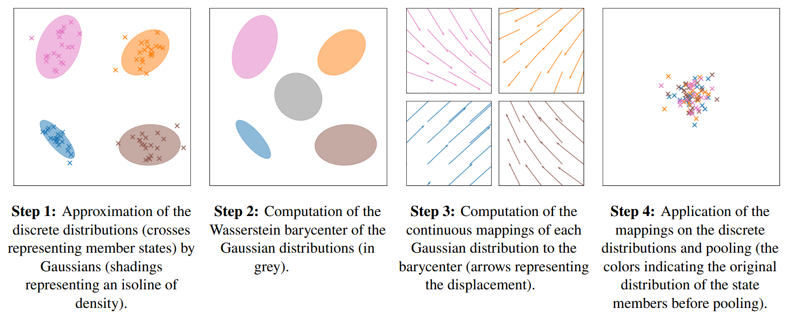
In order to avoid the variance shrinkage and have a more efficient and better statistical estimation, we propose to estimate the barycenter using a Gaussian approximation of the data and then to “map” all forecast onto this barycenter using the Gaussian mapping. That is, a Gaussian assumption is made to estimate a Gaussian Wasserstein barycenter which provides a closed-form affine mapping from each distribution to the barycenter, and then this mapping is applied to the discrete distributions which aligns them on the barycenter but keeps their individual samples. This means that only the first- and second-order moments of the Gaussian are estimated from the data which attenuates the statistical difficulty of estimating the Wasserstein distance (Flamary et al., 2020). This approach was first used in Gnassounou et al. (2023) for data normalization of biomedical signals. Note that they additionally assumed the signal to be stationary and periodic to simplify the computations, however, these hypotheses are not appropriate to our dataset. The method is illustrated in Fig. 1 and is made up of four steps:

1. Each discrete distribution μ_k is approximated by a multivariate normal distribution ${\widehat{\mathit{\mu }}}_k$ of mean ${\widehat{\mathit{m}}}_k$ and covariance ${\widehat{\mathbf{\Sigma }}}_k$ (for $k=\mathrm{1},\mathrm{\dots },K$), which are estimated by the unbiased sample mean and covariance respectively.

   Note: in this study, the multivariate distribution does not represent the joint distribution between several meteorological variables, but the joint distribution between different time steps of the same meteorological variable (see Sect. 2.1).

2. The Wasserstein barycenter between the normal distributions is computed. It is also a multivariate normal distribution with mean ${\widehat{\mathit{m}}}_b={\sum }_{k=\mathrm{1}}^K{\mathit{\lambda }}_k{\widehat{\mathit{m}}}_k$ and covariance ${\widehat{\mathbf{\Sigma }}}_b$ that is estimated iteratively using the fixed-point iteration ${\widehat{\mathbf{\Sigma }}}_b={\sum }_{k=\mathrm{1}}^K{\mathit{\lambda }}_k({\widehat{\mathbf{\Sigma }}}_b^{\mathrm{1}/\mathrm{2}}{\widehat{\mathbf{\Sigma }}}_k^{\mathrm{1}/\mathrm{2}}{\widehat{\mathbf{\Sigma }}}_b^{\mathrm{1}/\mathrm{2}}{)}^{\mathrm{1}/\mathrm{2}}$ from Agueh and Carlier (2011).

3. The optimal transports from each input Gaussian distribution ${\widehat{\mathit{\mu }}}_k$ to the Gaussian barycenter ${\widehat{\mathit{\mu }}}_b$ are derived. They are given by the following affine mappings $T_k\left(\mathit{x}\right)={\mathbf{A}}_k(\mathit{x}-{\widehat{\mathit{m}}}_k)+{\widehat{\mathit{m}}}_b$ with ${\mathbf{A}}_k={\widehat{\mathbf{\Sigma }}}_k^{-\mathrm{1}/\mathrm{2}}({\widehat{\mathbf{\Sigma }}}_k^{\mathrm{1}/\mathrm{2}}{\widehat{\mathbf{\Sigma }}}_b{\widehat{\mathbf{\Sigma }}}_k^{\mathrm{1}/\mathrm{2}}{)}^{\mathrm{1}/\mathrm{2}}{\widehat{\mathbf{\Sigma }}}_k^{-\mathrm{1}/\mathrm{2}}$ (assuming that the ${\widehat{\mathbf{\Sigma }}}_k$ are invertible, see below).

4. The mappings are applied to the corresponding discrete distributions (that is the mapping T_k is applied to each state member x_k,i of μ_k), and then the adapted distributions are pooled together (as for the L₂ barycenter in Eq. 3) to create the 2-Wasserstein barycenter with Gaussian mapping (GaussW₂ barycenter hereafter).

Figure 1 Illustration of the Wasserstein barycenter with Gaussian mapping approach.

This approach computes mappings and barycenters on continuous (multivariate normal) distributions, thereby avoiding variance shrinkage of the barycenters due to limited discrete sample sizes (see Appendix A). Computing the mean and covariance of a discrete distribution for the multivariate normal approximation is less sensitive to the sampling of the distributions (Gnassounou et al., 2023), and regularization can be used if needed to ensure the invertibility of the covariance matrices ${\widehat{\mathbf{\Sigma }}}_k$. This is especially important when the number of members (i.e. samples) is small compared to the number of dimensions. The approximation of the discrete distributions by multivariate normal distributions is a strong hypothesis considering that ensembles in climate science are propagated according to nonlinear evolution equations. However, this is a classical hypothesis for modeling stochastic processes and in signal processing. Moreover, this hypothesis is only used to derive Gaussian barycenter and the mappings which are then applied to the original discrete distributions which can be seen as a second-order calibration of the models onto a barycenter which preserves higher-order moments through the individual samples. For variables with a strongly non-Gaussian distribution (such as precipitation), it is also possible to first apply a transformation to make the distribution more Gaussian (e.g., using Gaussian anamorphosis; see Bertino et al., 2003; Lussana et al., 2021), compute the barycenter in the transformed space, and then apply the inverse transform.

Another advantage of this approach is the computational cost (in low dimensions). Estimating the parameters of the multivariate normal distribution from the discrete one has a computational complexity of 𝒪(Nd²) (where N is the number of points in the discrete distribution, and d the number of dimensions, here d=n_t lead times). The Gaussian mappings and Gaussian barycenter computation have a complexity of 𝒪(d³) and $\mathcal{O}\left(d^{\mathrm{3}}\log \right(\mathrm{1}/\mathit{ϵ}\left)\right)$ respectively (where ϵ is the tolerance in the fixed-point algorithm). On the other hand, computing the exact barycenter requires multiple resolutions (per model and iteration) of exact optimal transport problems 𝒪(N³log (N)) (Agueh and Carlier, 2011).

2.2.3 Illustration of the application of barycenters to ensemble forecasts

The L₂ and W₂ distances have different properties in the distribution space, leading to distinct multi-model ensembles. The L₂ distance focuses on the “vertical” differences between distributions. This means that the L₂ distance between two distributions with disjoint supports is equal to the sum of their L₂ norms, no matter how distant their supports are (e.g., it is equal to $\mathrm{2}{\sum }_i^N\mathrm{1}/N^{\mathrm{2}}$ for two discrete distributions with each N equiprobable points). As a result, the members of the L₂ barycenter always coincide with the members of the initial ensembles, regardless of the distance between the supports of the input distributions. This means that the members of the L₂ barycenter are physically consistent, according to the numerical weather model they were drawn from. In contrast, the GaussW₂ distance is a “horizontal” measure of the difference between two distributions, in the sense that it is based on the horizontal displacement (or mapping) between them (Santambrogio, 2015). This enables the associated GaussW₂ barycenter to have a different support than the input distributions. In practice, that means that the members of the GaussW₂ barycenter do not coincide with any of the input ensemble members. Although the covariance structures of the inputs are still taken into account, they are merged (step 2 of the method in Sect. 2.2.2), allowing the barycenter to contain forecasts that could not have been generated by the individual models. The GaussW₂ barycenter is thus more flexible, but does not guarantee the same level of physical consistency as the L₂ barycenter.

Figure 2 gives an illustration of the two barycenters applied to the combination of two synthetic ensemble forecasts with N₁=10 and N₂=15 members respectively. The members of the L₂ barycenter in Fig. 2b correspond to the members of the input ensembles in Fig. 2a. The weight of each member of the L₂ barycenter is given by the weight of the corresponding member in the input ensemble ($\mathrm{1}/N_{\mathrm{1}}$ or $\mathrm{1}/N_{\mathrm{2}}$) multiplied by the corresponding model's weight (here ${\mathit{\lambda }}_{\mathrm{1}}={\mathit{\lambda }}_{\mathrm{2}}=\mathrm{0.5}$). The GaussW₂ barycenter shown in Fig. 2c has a different structure compared to the L₂ barycenter. As expected, a major difference is that none of its members belong to the input ensembles. In other words, while the support of the L₂ barycenter is the union of the input supports, the support of the GaussW₂ barycenter lies along the path of the optimal transport and can therefore be different. This also allows for the GaussW₂ barycenter to retain certain characteristics of the input distributions. For example, in this illustrative case, both input distributions are unimodal, and so is the GaussW₂ barycenter. This is not the case for the L₂ barycenter which has two modes, each associated with the mode of one of the input distributions. The two barycenters may be attractive for different types of forecasts. The GaussW₂ barycenter preserves some geometric properties of the input distributions, while the L₂ barycenter retains bimodality. Actual forecasts are more complex, and assessing the different barycenters will require extensive testing with different criteria. The purpose of Fig. 2 is to emphasize the (hitherto largely untapped) variety of ways to build multi-model ensemble forecasts.

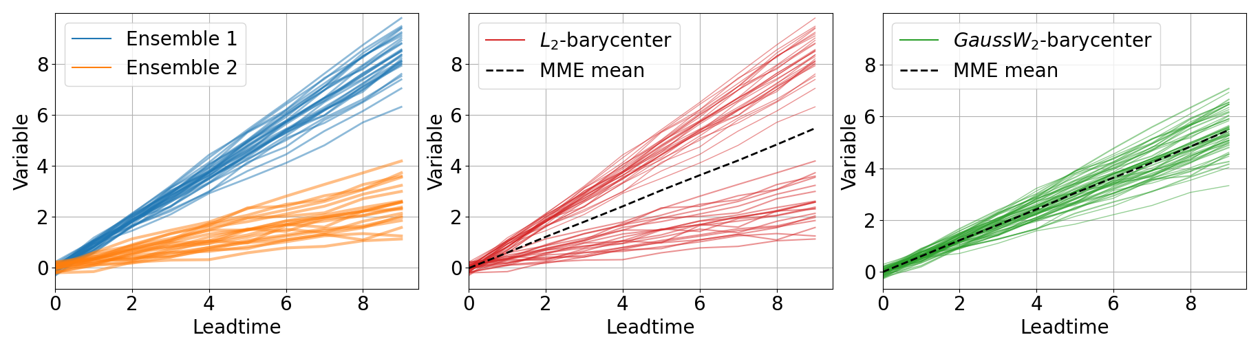
Figure 2 Illustration of (equal-weights) multi-model ensembles using barycenters for a synthetic variable. The ensemble can be seen as a discrete distribution whose points are the time series of each member. The weight of the points in the distribution is indicated here by the thickness of the line.

An important fact to note is that, despite their differences, the two barycenters have the same ensemble means (for the same model weights). Their mean is equal to the weighted mean of the input distributions's means (this follows easily from Eq. 3 for the L₂ barycenter, and see Peyré and Cuturi (2020, Remark 9.1) for the W₂ and GaussW₂ barycenters). Thus, the difference between the barycenters is how they represent the forecast uncertainty. This raises the question: how different are the L₂ and GaussW₂ distributions, and which one captures forecast uncertainty better? We address this question empirically for a particular case study in the next sections.

3 Data and methodology

In this study, we focus on subseasonal forecasts over Europe during the boreal winter. We consider one large-scale and two surface variables: the geopotential height at 500 hPa (z₅₀₀), the daily temperature at 2 m (t2m), and the wind speed at 10 m (w10 m). The latter two variables are interesting to predict for the energy sector, as energy demand is particularly dependent on the temperature in winter (due to the use of electrical heating), while the wind speed is an essential variable for estimating wind farm production. The geopotential height at 500 hPa is included as a traditional large-scale variable for comparison.

3.1 Data

To make predictions for this case study and to validate them, we need both a dataset of ensemble forecasts from multiple dynamical models, to which the barycenters will be applied and a reference dataset against which the forecast skill will be evaluated.

3.1.1 S2S data

For this first implementation, we selected four models from the S2S database (Vitart et al., 2017): the European Centre for Medium-Range Weather Forecasts (ECMWF) model, the National Centers for Environmental Prediction (NCEP) model, the Environment and Climate Change Canada (ECCC) model, and the Korea Meteorological Administration (KMA) model. An important criterion in model selection is their diversity. As previously explained, one advantage of using multi-model ensemble is to better sample model error. If the models have similar construction, this error is not sampled properly. Other criteria include time coverage and consistency in production over the study period.

Table 1 Description of the four models from the S2S database (characteristics for the period used). See Vitart et al. (2017) for more details.

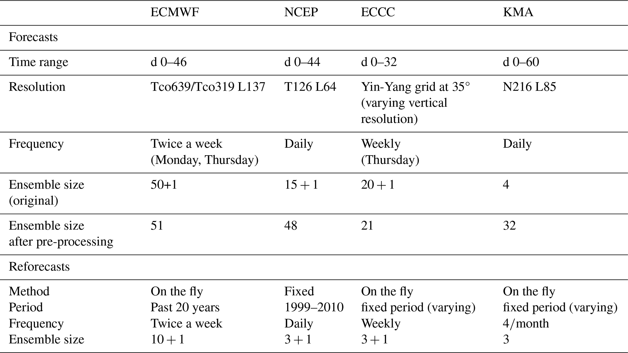
The forecasts and reforecasts from the selected models were retrieved from the S2S database through the ECMWF's Meteorological Archival and Retrieval System (MARS) directly on a 1.5°×1.5° grid for our study domain shown in Fig. 3, that is Europe (34–74° N, 13° W–40° E). We retrieved the daily mean 2 m temperature, the instantaneous values of the 10 m wind speed, and the 500 hPa geopotential height at midnight (00Z). We selected the forecasts initialized during the winter months (December–January–February, DJF) for the 2016–2022 period, for which the four models have matching initialization dates. This resulted in a total of 90 simulations spanning seven winters. After pre-processing (described below), the forecasts were resampled to weekly means. The barycenter-based MME methods were applied to the weekly time series (i.e., n_t=4 weeks), which was also the temporal resolution used for forecast evaluation.

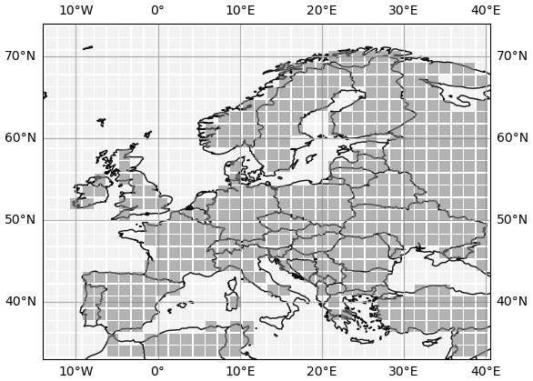
Figure 3 Study domain with the 1.5°×1.5° lat/lon grid from the forecasts. Only the land points (in grey) are used in this case study.

Pre-processing

• The forecasts from the four models are calibrated using the Mean and Variance Adjustment (MVA, Leung et al., 1999; Manzanas et al., 2019) method, following Goutham et al. (2022). Ensemble forecasts suffer from systematic errors (e.g. mean bias) due to uncertainties in ensemble initialization and model formulation. In particular, forecasts tend to drift away from the observed climate toward the model climatology as lead time increases (Takaya, 2019), making statistical correction essential at extended-range time scales.

  The model climatology is estimated from reforecasts, which are “retrospective” forecasts generated with the same model but for past dates. The observed climatology is derived from a reference dataset (see Sect. 3.1.2 below). The calibration method (MVA here) is then applied to statistically adjust the forecasts. To ensure a robust estimation of the climatologies, we aggregate all forecasts initialized within a 15 d window, comprising the same calendar day as the forecast starting date and the previous 14 d¹ (Manrique-Suñén et al., 2020). The observed climatology is computed on the same dates for consistency.

• The NCEP and KMA models have smaller ensemble sizes but are produced daily. We thus create a lagged ensemble by aggregating the forecasts with those initialized the two preceding days for NCEP and the seven preceding days for KMA. This allows us to improve their skill and to increase their ensemble size, making them more comparable to the other models (48 and 32 members for NCEP and KMA, respectively after lagging). The ECCC model has a smaller ensemble size than ECMWF and the lagged NCEP and KMA models. However, lagging is not applied to it because of its production frequency (it is only produced weekly).

3.1.2 Reference data

The Modern-Era Retrospective analysis for Research and Applications, version 2 (MERRA-2, Gelaro et al., 2017) reanalysis is used as reference for calibration and forecast validation. We use a reanalysis as reference in order to have a spatially and temporally complete dataset. MERRA-2 was chosen because it is a recent reanalysis covering both the calibration and validation periods and is based on a different circulation model from those used in the selected S2S models. This would not be the case, for example, with the ERA5 reanalysis which is also produced by the ECMWF with a similar model as the S2S forecasts (Hersbach et al., 2020). The three variables of interest were retrieved from NASA Goddard Earth Sciences (GES) Data and Information Services Center (DISC) on MERRA-2's native grid (0.5° lat ×0.625° lon grid). The data were re-gridded to match the 1.5°×1.5° lat/lon grid of the forecasts using bilinear interpolation with the Climate Data Operators (CDO, Schulzweida, 2022).

We also use MERRA-2 to build a 30 year rolling climatology. The climatology is a common benchmark for forecast validation, and it is also used to compute skill scores (see Sect. 3.2). For a given day of the year, the climatology consists of MERRA-2 values for the same day over the previous 30 years. The climatology is thus an ensemble with 30 members, each corresponding to a different year.

3.2 Evaluation

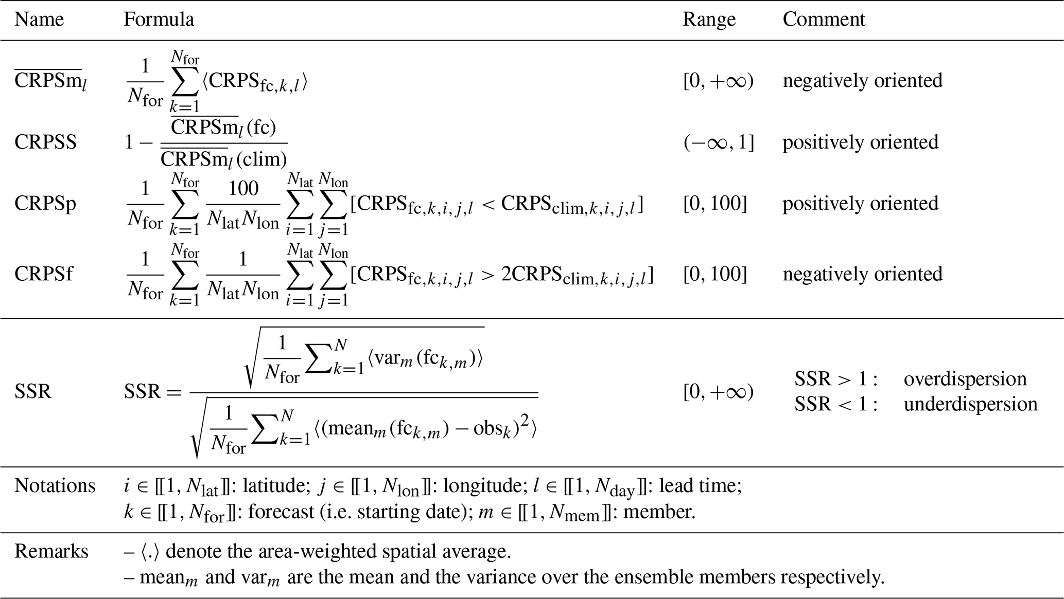
We now introduce the evaluation scores used in this study. We use the Continuous Ranked Probability Score and related skill scores to evaluate the accuracy of the forecasts, and the Spread-Skill Ratio to investigate their calibration. Due to the low number of samples in our case study (90 simulations), we do not investigate the prediction of extreme events. All scores used in this study are summarized in Table 2.

3.2.1 Continuous Ranked Probability Score (CRPS)

The CRPS is a widely used score for probabilistic forecasts of continuous variables (Matheson and Winkler, 1976; Gneiting and Raftery, 2007; Wilks, 2019). The CRPS is actually the squared L₂ distance between the Cumulative Distribution Function (CDF) of the ensemble forecast, and the CDF of the observation:

$$\begin{array}{}\text{(5)}& {\text{CRPS}}_n=\underset{-\mathrm{\infty }}{\overset{+\mathrm{\infty }}{\int }}\left[F_{\text{fc},n}\right(y)-F_{\text{ref},n}(y){]}^{\mathrm{2}}\mathrm{d}y\end{array}$$

where F_fc is the CDF of the forecast, F_ref is the CDF of the observation and $n\in \left[\right[\mathrm{1},N\left]\right]$ is the ensemble member index. The CDFs are computed empirically from the ensembles. In general the reference is deterministic, and its CDF is then a step function $F_{\text{ref}}\left(y\right)={\mathbf{1}}_{y\ge x_{\text{ref}}}$, where x_ref is the deterministic value of the reference.

The accuracy of the ensembles is evaluated by computing the mean CRPS (over the forecasts indexed by n). For easier comparison across variables, we use the Continuous Ranked Probability Skill Score (CRPSS) which compares the mean CRPS of the ensemble forecast to the mean CRPS of the climatology, but statistical tests will be performed on the CRPS distribution.

We consider two other scores based on the CRPS. To evaluate robustness to outliers, we use the proportion of skillful forecasts (hereafter CRPSp), which corresponds to the percentage of simulations for which the model has a better CRPS than the climatology (Goutham et al., 2022). We consider that the model has some skill if 50 % of the forecasts are skillful. As a counterpart, we introduce a third score that focuses on the tail of the distribution (i.e. forecasts far from the truth). The proportion of critical failures (CRPSf) is defined as the percentage of simulations for which the model has a CRPS_n larger than twice that of the climatology (this metric is thus negatively oriented, contrary to the CRPSS and CRPSp). The CRPSp and CRPSf should be interpreted together.

Remarks on the links between the CRPS and the L₂ barycenter:

• It is interesting to note that for univariate distributions, the L₂ barycenter is also the barycenter with respect to the energy distance (see Appendix B). Thus, since the CRPS is identical to the energy distance in 1D (see Wilks, 2019), we can expect good CRPS performance for the L₂ barycenter.

  For symmetry, the Wasserstein distance could also be used as a score for forecast validation. However, it is equivalent to the RMSE (averaged over the members) in the case of a deterministic observation and so it does not evaluate well the representation of the uncertainties in the forecasts. Thus, we do not use it here.

• The CRPS of the L₂ barycenter ${\mathit{\mu }}_{L_{\mathrm{2}}}^{\mathit{\alpha }}$ of the distributions $({\mathit{\mu }}_{\mathrm{1}},\mathrm{\dots },{\mathit{\mu }}_d)$ (with weights ${\mathit{\lambda }}_{\mathrm{1}},\mathrm{\dots },{\mathit{\lambda }}_d$) can be expressed as a function of their CRPS with respect to the observation and their cross-CRPS:

  $$\begin{array}{}\text{(6)}& \begin{array}{rl}{\displaystyle }\text{CRPS}({\mathit{\mu }}_{L\mathrm{2}},{\mathit{\nu }}_{\text{obs}})& {\displaystyle }={\sum }_{i=\mathrm{1}}^n{\mathit{\lambda }}_i\text{CRPS}({\mathit{\mu }}_i,{\mathit{\nu }}_{\text{obs}})\\ {\displaystyle }& {\displaystyle }-{\sum }_{i=\mathrm{1}}^n\sum _{j\ne i}{\displaystyle \frac{\mathrm{1}}{\mathrm{2}}}{\mathit{\lambda }}_i{\mathit{\lambda }}_j\text{CRPS}({\mathit{\mu }}_i,{\mathit{\mu }}_j)\end{array}\end{array}$$

  where ν_obs is the observation (see Appendix C). This expression clearly shows that the CRPS of the L₂ barycenter is always smaller than the average CRPS of the input distributions. In fact, the more different the input distributions are (i.e., large cross-CRPS), the more advantageous it is to merge them.

3.2.2 Spread-skill ratio

The CRPS evaluates the accuracy of the forecasts, that is, their overall quality (Wilks, 2019). In order to focus on the calibration (or reliability) of the ensembles, we also look at the spread-skill ratio (SSR) defined as the ratio of the ensemble standard deviation to the root mean square error RMSE of the ensemble mean. A perfectly reliable ensemble has a SSR equal to one, while larger SSR values indicates overdispersion and smaller values underdispersion (Fortin et al., 2014). The SSR can be used as a first evaluation of an ensemble's reliability (a value of 1 is necessary, though not sufficient, for a fully reliable ensemble).

Table 2 Scores used for evaluation.

4 Results

In this section, we evaluate the combination of four models' ensembles applying the two barycenter-based MME methods described in Sect. 2 to the case study described in Sect. 3. All the results shown here are obtained for barycenters with equal weights (that is ${\mathit{\lambda }}_{\text{ECMWF}},{\mathit{\lambda }}_{\text{NCEP}},{\mathit{\lambda }}_{\text{ECCC}},{\mathit{\lambda }}_{\text{KMA}}=\mathrm{1}/\mathrm{4}$). We tested optimizing the weights with respect to the CRPS, but it leads to either little improvement or slight deterioration of the forecast skill depending on the variables and scores (not shown here).

4.1 Validation and comparison of the barycenter-based MME

Figure 4 summarizes the performance of the four SMEs and the two barycenter-based MMEs. For the latter, the bars represent the performance of the barycenters combining the four SMEs (the hatched areas represent the performance of the barycenters of three SMEs out of four; these results are discussed below, Sect. 4.3). The distribution of the scores (CRPSS, CRPSp and CRPSf) over the starting dates is represented by its mean in the plot, and is used to test if the models' scores are significantly different from each other at a 5 % significance level. The significance is estimated using the Wilcoxon signed-rank test, a non-parametric paired statistical test (Wilcoxon, 1945). We chose to show the CRPSS here instead of the mean CRPS for an easier comparison across variables. However, the mean and the statistical tests are computed on the (spatially averaged) CRPS distributions. The p-values of these statistical tests are shown in Appendix D.

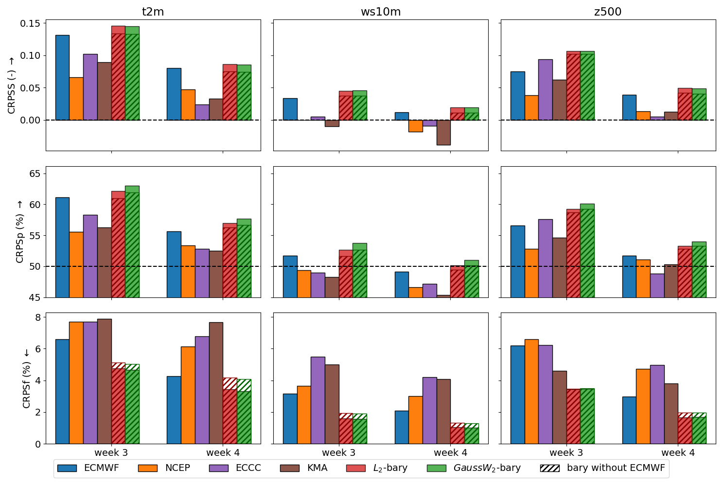
Figure 4 Skill scores for the weekly 2 m temperature (left), 10 m wind speed (center) and geopotential height at 500 hPa (right): the CRPSS (top), the proportion of skillful forecasts (CRPSp, middle) and proportion of critical failure (CRPSf, bottom).

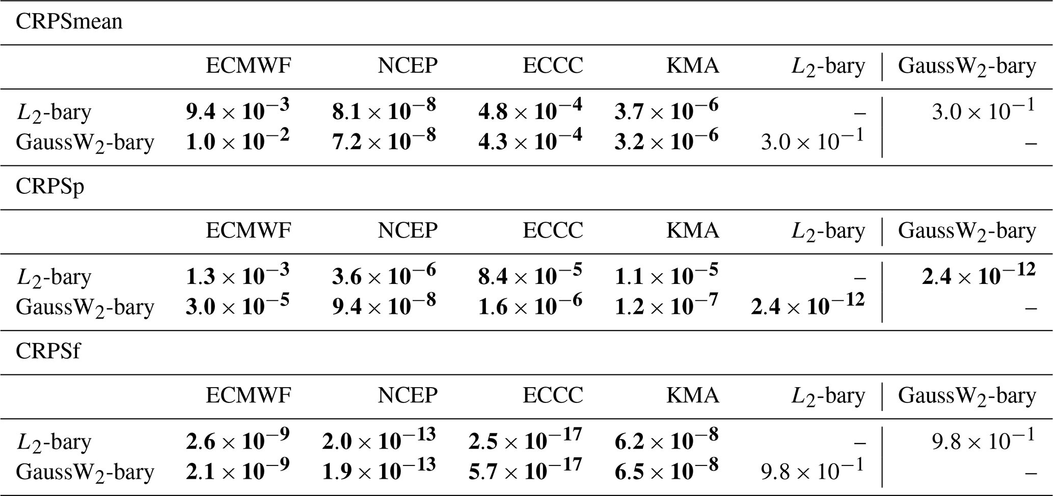
For all three variables and three scores, the two barycenters outperformed the SMEs, however the gain with respect to the best performing SME is sometimes small. In particular, ECMWF has the best performance among the four SMEs for the surface variables, the 2 m temperature and the 10 m wind speed. In terms of CRPSS, the two barycenters have similar values and are significantly different from all the SMEs for the 10 m wind speed and the geopotential height (see Tables D2 and D3). Even though two or three of the models (depending on the week) have a negative CRPSS for the 10 m wind speed, merging them with more skillful SMEs still adds value: the barycenters have a significantly better CRPSS. For the 2 m temperature, the barycenters do not have a significantly different CRPSS than ECMWF, which already has a relatively large CRPSS (see Table D1).

In terms of CRPSp, the GaussW₂ barycenter is significantly better than the others, including the L₂ barycenter that ranks second (Tables D1, D2 and  D3). That is, the barycenters, and especially the GaussW₂ barycenter, are more often better than the climatology compared to the SMEs. The barycenter-based ensembles also significantly reduce the risk of large failures as shown by their lower CRPSf. The two barycenters have similar CRPSf values, clearly lower than the values of the SMEs. In particular, the proportion of critical failures is divided by almost two for the 10 m wind speed compared to the best SME, ECMWF.

Variations in scores across the spatial domain for each model are large, in the sense that they tend to dominate over differences between models (not shown here). We thus expect this to be also the case for the MMEs. Figure 5 shows the differences between ECMWF and the GaussW₂ barycenter's scores. We chose ECMWF as a reference, since it has the best performance among the SMEs for two of the three variables (the surface ones). The map of the differences between the L₂ barycenter and ECMWF is very similar, and so is not shown here. For the CRPSS, one can see clear areas that benefit from the MMEs, but these areas are not the same depending on the variables. For the 2 m temperature, the barycenter is more advantageous in the North-West, above the North Sea, Atlantic Ocean and Scandinavia. ECMWF is better above Sweden and Finland for the 10 m wind speed. For this variable, the barycenter benefits more in central Europe as well as southern and eastern Europe. The spatial pattern is smoother for the geopotential height, with the largest differences above northern Europe, where the barycenter is more skillful. Despite these spatial variations across the three variables, the barycenter outperforms ECMWF at a majority of grid points.

Figure 5 Maps of the differences between ECMWF and GaussW₂ barycenter in terms of (top) CRPSS, (middle) CRPSp, and (bottom) CRPSf averaged over weeks 3 and 4. Green indicates that GaussW₂ barycenter performs better and pink that ECMWF does. For readability reason, a discrete colorbar is used for the ΔCRPSp and ΔCRPSf which are more pixelized. Dots indicate grid points where the difference is statistically significant at the 5 % level (using a two-sided Wilcoxon signed rank test for the CRPS and a McNemar test for the CRPSp and CRPSf).

The maps for the CRPSp differences are more pixelated, however the positive and negative areas roughly match those of the CRPSS differences. In contrast, the maps of the CRPSf differences show very different spatial patterns. For example, ECMWF performs better over Spain for the two surface variables for both the CRPSS and the CRPSp, but the barycenter has a better CRPSf there. In fact, the barycenter outperforms ECMWF in terms of CRPSf almost everywhere. This means that combining ensemble forecasts has a stabilizing effect, avoiding extremely bad forecasts. However, the differences are relatively small, less than 3 % at most grid points.

4.2 Ensembles calibration

In order to get insight into the calibration of the ensemble forecasts, we look at their SSR maps in Fig. 6. The spatial patterns of weeks 3 and 4 being similar, only their average is shown here. The spatial patterns are consistent across the SMEs. They tend to be under- or over-confident in the same regions, but with different intensities. For example, all models are over-dispersed over Scandinavia for the 2 m temperature forecasts, with KMA having the least and ECCC the most overdispersion. On the contrary, they are all under-dispersed over the Mediterranean Sea.

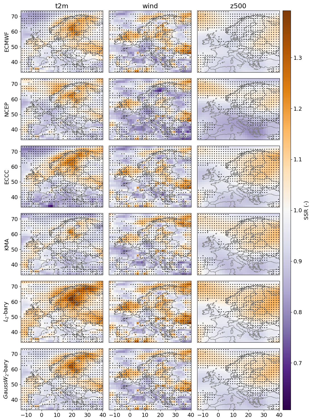
Figure 6 Spread-Skill-Ratio (SSR) for the weekly 2 m temperature (left), 10 m wind speed (center) and geopotential height at 500 hPa (right) averaged over weeks 3 and 4 for the four single-model ensembles and the two barycenters. Orange indicates overdispersion (i.e. under-confident forecasts), and blue under-dispersion (i.e. overconfident forecasts). Dots indicate grid points where the ensemble variance and MSE of the ensemble mean are are statistically different at the 5 % level (using a two-sided Wilcoxon signed rank test on the distribution of variance and MSE).

Note that, by construction, the barycenters have the same ensemble mean and so the same RMSE, so that the differences in their SSR are only due to their spread. Their SSRs have similar patterns as the SMEs. However, one can notice that the L₂ barycenter tends to have more spread than the GaussW₂ barycenter: it shows more overdispersion and less underdispersion. This can be explained by the way they were constructed. The variance of the L₂ barycenter is indeed given by

$$\begin{array}{}\text{(7)}& \text{Var}\left({\mathit{\mu }}_{L_{\mathrm{2}}}\right)=\sum _{i=\mathrm{1}}^d{\mathit{\lambda }}_i\text{Var}\left({\mathit{\mu }}_i\right)+\sum _{i=\mathrm{1}}^k{\mathit{\lambda }}_i{\left(\stackrel{\mathrm{‾}}{{\mathit{\mu }}_i}-\sum _{j=\mathrm{1}}^k{\mathit{\lambda }}_j\stackrel{\mathrm{‾}}{{\mathit{\mu }}_j}\right)}^{\mathrm{2}},\end{array}$$

where ${\stackrel{\mathrm{‾}}{\mathit{\mu }}}_i$ is the mean of the distribution μ_i. The variance of the barycenter is thus always equal to or higher than the average of the SME's variances. This property is advantageous in the case of under-dispersed input ensembles. However, it is a disadvantage if they are better calibrated or already over-dispersed (e.g. Zhou et al., 2022; Eade et al., 2014). In those cases, the GaussW₂ barycenter is more advantageous. In order to build it, the input ensembles are first centered and their covariances scaled before being pooled together. Thus, its covariance is the one of the Gaussian barycenter (Sect. 2.2.2).

4.3 MME without ECMWF

In Sect. 4.1, ECMWF is found to be more skillful than the other three SMEs for the two surface variables. Moreover, although the two barycenters have overall better performance, ECMWF is still better in some regions. Thus, to investigate the importance of ECMWF within the combination, we compute the barycenters of NCEP, ECCC and KMA (without ECMWF). They are compared to the barycenters with ECMWF in Fig. 4 (hatched bars). As expected, we observe a decrease in performance for all scores and variables. This is also true for most grid points when looking at the maps of differences except for those points where the barycenters (with four models) are notably more skillful than ECMWF (not shown here).

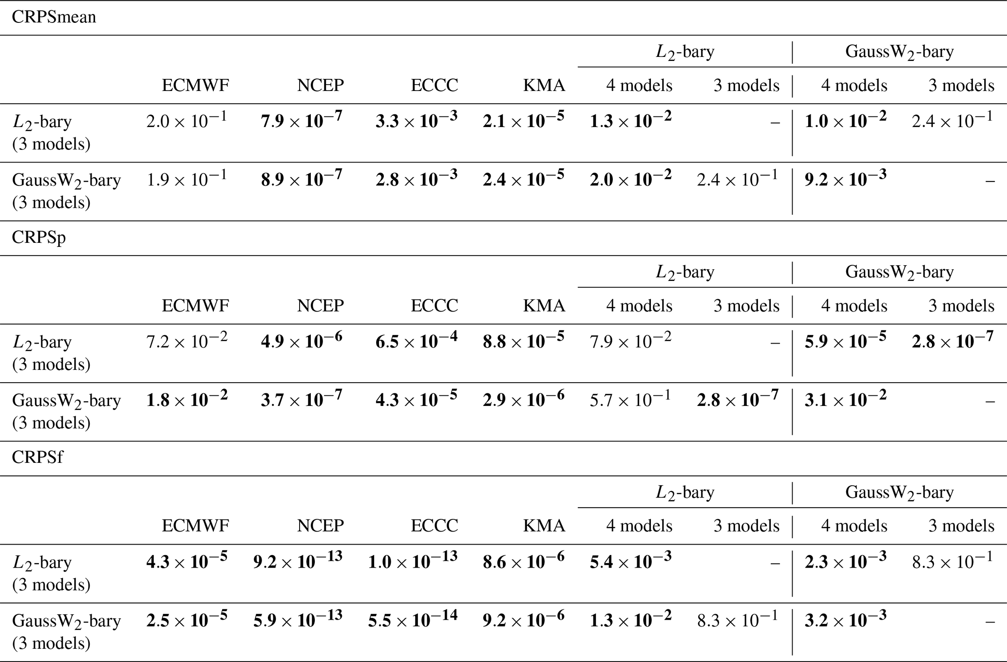
When comparing the barycenters with the three SMEs used to build them, we can make similar observations as in Sect. 4.1. Specifically, the L₂ and GaussW₂ barycenters have similar CRPSS and CRPSf, but the GaussW₂ barycenter has a significantly better CRPSp (at the 5 % level, Tables D4–D6). Both barycenters also outperform the three SMEs for all metrics. However, two features are noteworthy. First, the CRPSS and CRPSp differences between the barycenters and the SMEs for the surface variables are notably larger than those observed between the barycenters with four models and ECMWF. A particularly striking example is the CRPSS of the 10 m wind speed: while the three SMEs show little to no skill, with very low or even negative CRPSS, their barycenters have CRPSS similar to ECMWF's. Second, the barycenters with only three models are performing as well as ECMWF in terms of CRPSS and CRPSp (there are no significant statistical differences, see Appendix D2) and better in terms of CRPSf. Thus, with three less skillful models, one can reproduce the considerably better performance of ECMWF in the case studied here.

5 Discussion

5.1 L₂ barycenter versus GaussW₂ barycenter

We have seen that the MMEs improve the average forecast skill compared to the SMEs with respect to all scores and for all the variables considered, even though a SME may perform better at some locations. In general, the two barycenters have similar CRPSS and CRPSf, but the GaussW₂ barycenter has a better CRPSp. In other words, the two barycenters are similar on average, but the GaussW₂ is better more often without leading to an increase in very poor forecasts (with respect to the CRPS). Another important difference between the barycenters is the way they represent forecast uncertainty through their ensemble spreads. The L₂ barycenter always has a larger ensemble spread than the GaussW₂ barycenter, which in turn has an impact on their reliability.

The two barycenters have the same means (which only depend on the means of the input distributions), but their covariances differ. The covariances of the Wasserstein barycenter depend solely on the covariances of the input ensembles (see Sect. 2), while the covariances of the L₂ barycenter depend on both their means and their variances. If we assume that the variances of the input ensembles represent the uncertainty due to their initial conditions, their average in the formula of the L₂ barycenter variance (first term of Eq. 7) can be interpreted as a measure of the MME's initial-condition uncertainty. The second term, the variance of the input ensemble means, can be seen as a measure of model uncertainty as it quantifies the differences between ensemble (means). Thus, the variance of the L₂ barycenter accounts for model errors but ignores differences in higher moments than the ensemble mean. On the other hand, the GaussW₂ barycenter merges the forecast uncertainties of the different models (i.e. the uncertainty due to the initial conditions). Instead, information about model uncertainty lies in the value of the barycenter distance: ${min}_{\mathit{\mu }}{\sum }_{k=\mathrm{1}}^d{\mathit{\lambda }}_k.d({\mathit{\mu }}_k,\mathit{\mu }{)}^{\mathrm{2}}$. This information is not exploited here, but it could be considered to account for model uncertainty. Finally, not only are dynamical and model uncertainties captured by different quantities for the two barycenters (variance of the barycenter versus barycenter distance), but the way they are measured also differs. Understanding the implications of these differences requires further investigation.

5.2 Best model versus models combination

There can be several reasons why merging ECMWF with less skillful models leads to barycenters with improved performance. First, the three SMEs have generally less skill than ECMWF, but can be occasionally better for some given locations, lead times, or initialization dates. The barycenters can exploit this information to improve skill thanks to error cancellation and to the non-linearity of the skill metrics (Hagedorn et al., 2005). Second, the ECMWF forecasts may have good performance but be overconfident. In that case, adding other models with lower skill increases the spread of the ensemble and can move the ensemble mean towards the truth, as shown by Weigel et al. (2008) for seasonal ensemble forecasts. For the L₂ barycenter, this can be seen from Eq. (6) which shows that the CRPS of the L₂ barycenter is composed of two parts: the weighted average of the CRPS of the SMEs minus the weighted average of the CRPS between all pairs of SMEs. Thus, if one model has a worse CRPS than another, it can still improve the CRPS of the barycenter if the CRPS between the models is large enough to compensate for its own CRPS.

5.3 Weighted barycenters

Equal weighting of the models in the pooling method is the simplest and most used approach. However, some studies investigate the use of weighted multi-model ensembles with mixed results (at the weather or seasonal scale in Weigel et al. (2008); Casanova and Ahrens (2009); Kharin and Zwiers (2002) and at the climate scale in Haughton et al. (2015)). At the subseasonal scale, Wanders and Wood (2016) used mutivariable linear regression on the ensemble means to derive the multi-model weights. They show that the weighted muti-model ensemble has better deterministic performance but also better probabilistic performance (in terms of the Brier score) than the unweighted multi-model ensemble.

Here, we have shown results using equal weights for the models, but the barycenter formulation easily allows for the construction of weighted MMEs. Results for weights that do not depend on space or time, minimizing the mean CRPS, were also obtained but not shown because, contrary to Wanders and Wood (2016), no significant improvement was found. One explanation could be the limited time period used here. The collection of forecasts by the S2S database started in 2015. We thus have less than ten years of data, which may not be enough to find stable weights, as shown by Wanders and Wood (2016); Kharin and Zwiers (2002). Using reforecasts (instead of forecasts) would allow one to extend the time period. However, it would still be limited to twelve years (due to the limited NCEP reforecast period) and would lead to additional difficulties. In particular, the starting dates of the reforecasts for the different models in the S2S database do not match. In addition, the reforecasts have fewer members than the forecasts, so the reforecast results may not be transferred to the forecasts without additional assumptions.

Yet, another strategy could be to allow the weights to depend on space. We indeed saw that even if the barycenters tend to be more skillful than the SMEs, they can be outperformed by ECMWF for some scores at some locations. This suggests that giving more weight to ECMWF in these regions would be beneficial. Similarly, even if the barycenter without ECMWF showed a general degradation of the scores compared to the barycenters with the four models, it did perform better in some specific regions. Thus, the barycenter with four models would benefit from giving less or no weight to ECMWF in these regions. However, optimizing weights grid point by grid point requires more data and may lead to spatial inconsistencies (Wanders and Wood, 2016; DelSole et al., 2013). An alternative would be to learn weights per region (such as in Wanders and Wood, 2016) or to enforce some spatial smoothness on the weights (also acting as regularization and helping with overfitting).

6 Conclusions

We explore methods to combine ensemble forecasts from multiple models based on barycenters of forecast ensembles. Building on the recognition of the relevance of probabilistic forecasts for S2S prediction, we work directly in the probability distribution space. That is, the ensemble forecasts are manipulated as discrete probability distributions. This allows us to use existing tools from this space and, in particular, the notion of barycenters. Here, we explore two barycenters based on different metrics: the L₂ distance and the Wasserstein (GaussW₂) distance. We show that the L₂ barycenter is in fact equivalent to the well-known pooling method and compare it to the new GaussW₂ barycenter-based method. Moreover, the variance of the L₂ barycenter can be decomposed into a term representing the average uncertainty of individual forecasts and a term representing model systematic error, while the variance of the GaussW₂ barycenter does not account for the latter. Instead, this information is captured by the values of the GaussW₂ barycenter.

This first application of our framework to S2S prediction is illustrated through the combination of four single-model ensembles to predict winter surface temperature, surface wind speed, and 500 hPa geopotential height over Europe. By construction, the two barycenters have the same ensemble means, which means they have the same performance in terms of deterministic scores. However, they differ in the way they represent forecast uncertainty. In particular, by construction, the L₂ barycenter is likely to be underconfident due to overdispersion, implying that the L₂ barycenter is advantageous in the case of under-dispersive input ensembles, but disadvantageous in terms of calibration otherwise. More generally, we show that both barycenters perform similarly on average but that the GaussW₂ barycenter performs better more often (across the different grid points and dates) with respect to the CRPS. Even in cases where one of the SMEs has superior skill compared to the others (ECMWF for the surface variables), it is still advantageous to combine them into a barycenter. This confirms the interest of multi-model methods shown by previous studies. We also show that by using the other three models, one can build barycenter-based MMEs that are as skillful as the best SME.

This study is a proof of concept to develop the framework and investigate the properties of the barycenter-based MMEs. These results constitute a promising first step towards improving S2S predictions using barycenters to merge ensemble forecasts. A next step would be to further investigate the optimization of the weights in the barycenter in order to build weighted MMEs. Another interesting question concerns the possibility of building multivariate Wasserstein barycenters. The L₂ barycenter does not take into account the covariances between the variables, whereas the Wasserstein barycenter does. Finally, the implications of the fact that both barycenters account differently for forecast and model uncertainty deserve further investigation.

Appendix A: Variance shrinkage in discrete Wasserstein barycenter

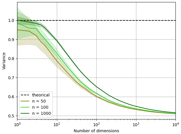
Figure A1 Average variance of the discrete Wasserstein barycenter as a function of the dimension d for different sample size n. The full line represents this variance averaged over the 100 iterations with the minimum and maximum values indicated by the envelop.

A potential problem of the discrete Wasserstein barycenter is its reduced variance. Indeed, computing the Wasserstein barycenter directly on discrete probability distributions leads to a variance shrinkage problem which worsens with increasing space dimension and decreasing distribution sampling. This problem can be illustrated with the following empirical experiment:

1. Create two discrete distributions by randomly drawing n samples from two normal distributions with unit-covariance in ℝ^d.

2. Compute the Wasserstein barycenter of the two discrete distributions (using the closed-form expression).

3. Compute the normalized trace of the covariance of the barycenter divided by the number of variables (that is, the average variance of the variables).

4. Repeat the three precedent steps 100 times.

We repeated this experiment for different sampling sizes n and number of dimensions d. The results of this experiment are shown in Fig. A1. By construction, the Wasserstein barycenter of the two normal distributions with unit covariance also has a unit-variance (and so an average variance of one). However, one can observe that the discrete barycenter has a lower average variance. The average variance shrinks as the sample size decreases and the number of dimensions increases. For four dimensions and 50 samples, we observe a loss of more than 10 % of the average variance. This setting is comparable to our application, where the number of dimensions d corresponds to the number of lead times (i.e. four weeks), and the number of samples n corresponds to the ensemble size (ranging from 21–51 members, see Sect. 3.1.1).

Appendix B: Energy distance and its associated barycenter

Let μ₁ and μ₂ be two distributions, and F₁ and F₂ be their CDF. That is, $F_{\mathrm{1}}\left(x\right)={\int }_{-\mathrm{\infty }}^x{\mathit{\mu }}_{\mathrm{1}}\left(t\right)\mathrm{d}t$ and $F_{\mathrm{2}}\left(x\right)={\int }_{-\mathrm{\infty }}^x{\mathit{\mu }}_{\mathrm{2}}\left(t\right)\mathrm{d}t\forall x\in \mathbb{R}$. The squared energy distance between μ₁ and μ₂ is

$$\begin{array}{rl}{\displaystyle }{\mathcal{E}}^{\mathrm{2}}({\mathit{\mu }}_{\mathrm{1}},{\mathit{\mu }}_{\mathrm{2}})& {\displaystyle }={\int }_{-\mathrm{\infty }}^{+\mathrm{\infty }}\left[F_{\mathrm{1}}\right(x)-F_{\mathrm{2}}(x){]}^{\mathrm{2}}\mathrm{d}x\\ {\displaystyle }& {\displaystyle }={\int }_{-\mathrm{\infty }}^{+\mathrm{\infty }}{\left[\underset{-\mathrm{\infty }}{\overset{x}{\int }}{\mathit{\mu }}_{\mathrm{1}}\left(t\right)\mathrm{d}t-\underset{-\mathrm{\infty }}{\overset{x}{\int }}{\mathit{\mu }}_{\mathrm{2}}\left(t\right)\mathrm{d}t\right]}^{\mathrm{2}}\mathrm{d}x\end{array}$$

The energy barycenter of μ₁ and μ₂ is the solution of the following minimization problem ${\mathit{\mu }}_{\mathcal{E}}^{\mathit{\alpha }}={\text{argmin}}_{\mathit{\mu }}\mathit{\alpha }{\mathcal{E}}^{\mathrm{2}}(\mathit{\mu },{\mathit{\mu }}_{\mathrm{1}})+(\mathrm{1}-\mathit{\alpha }){\mathcal{E}}^{\mathrm{2}}(\mathit{\mu },{\mathit{\mu }}_{\mathrm{2}})$. Let $\mathcal{B}\left(\mathit{\mu }\right)=\mathit{\alpha }{\mathcal{E}}^{\mathrm{2}}(\mathit{\mu },{\mathit{\mu }}_{\mathrm{1}})+(\mathrm{1}-\mathit{\alpha }){\mathcal{E}}^{\mathrm{2}}(\mathit{\mu },{\mathit{\mu }}_{\mathrm{2}})$, then we have:

$$\begin{array}{ll}{\displaystyle }& {\displaystyle }\begin{array}{rl}{\displaystyle \frac{\mathrm{d}}{\mathrm{d}\mathit{\mu }}}\mathcal{B}\left(\mathit{\mu }\right)=& {\displaystyle \frac{\mathrm{d}}{\mathrm{d}\mathit{\mu }}}\left[\mathit{\alpha }{\int }_{-\mathrm{\infty }}^{+\mathrm{\infty }}\left[F\right(x)-F_{\mathrm{1}}(x){]}^{\mathrm{2}}\mathrm{d}x+(\mathrm{1}-\mathit{\alpha })\right.\\ {\displaystyle }& {\displaystyle }\times \left.{\int }_{-\mathrm{\infty }}^{+\mathrm{\infty }}\left[F\right(x)-F_{\mathrm{2}}(x){]}^{\mathrm{2}}\mathrm{d}x\right]\end{array}\\ {\displaystyle }& {\displaystyle }\begin{array}{rl}{\displaystyle }=& {\displaystyle \frac{\mathrm{d}}{\mathrm{d}\mathit{\mu }}}{\int }_{-\mathrm{\infty }}^{+\mathrm{\infty }}\left(\mathit{\alpha }{\left[\underset{-\mathrm{\infty }}{\overset{x}{\int }}\mathit{\mu }\left(t\right)\mathrm{d}t-\underset{-\mathrm{\infty }}{\overset{x}{\int }}{\mathit{\mu }}_{\mathrm{1}}\left(t\right)\mathrm{d}t\right]}^{\mathrm{2}}\right.\\ {\displaystyle }& {\displaystyle }\left.+(\mathrm{1}-\mathit{\alpha }){\left[\underset{-\mathrm{\infty }}{\overset{x}{\int }}\mathit{\mu }\left(t\right)\mathrm{d}t-\underset{-\mathrm{\infty }}{\overset{x}{\int }}{\mathit{\mu }}_{\mathrm{2}}\left(t\right)\mathrm{d}t\right]}^{\mathrm{2}}\right)\mathrm{d}x\end{array}\\ {\displaystyle }& {\displaystyle }\begin{array}{rl}{\displaystyle }=& {\displaystyle }{\int }_{-\mathrm{\infty }}^{+\mathrm{\infty }}{\displaystyle \frac{\mathrm{d}}{\mathrm{d}\mathit{\mu }}}\left(\mathit{\alpha }{\left[\underset{-\mathrm{\infty }}{\overset{x}{\int }}\left(\mathit{\mu }\right(t)-{\mathit{\mu }}_{\mathrm{1}}(t\left)\right)\mathrm{d}t\right]}^{\mathrm{2}}\right.\\ {\displaystyle }& {\displaystyle }\left.+(\mathrm{1}-\mathit{\alpha }){\left[\underset{-\mathrm{\infty }}{\overset{x}{\int }}\left(\mathit{\mu }\right(t)-{\mathit{\mu }}_{\mathrm{2}}(t\left)\right)\mathrm{d}t\right]}^{\mathrm{2}}\right)\mathrm{d}x\end{array}\\ {\displaystyle }& {\displaystyle }\begin{array}{rl}{\displaystyle }=& {\displaystyle }{\int }_{-\mathrm{\infty }}^{+\mathrm{\infty }}\left(\mathrm{2}\mathit{\alpha }{\int }_{-\mathrm{\infty }}^x\left[\mathit{\mu }\right(t)-{\mathit{\mu }}_{\mathrm{1}}(t\left)\right]\mathrm{d}t\mathit{\mu }\left(x\right)\right)\mathrm{d}x\\ {\displaystyle }& {\displaystyle }+{\int }_{-\mathrm{\infty }}^{+\mathrm{\infty }}\left(\mathrm{2}(\mathrm{1}-\mathit{\alpha }){\int }_{-\mathrm{\infty }}^x\left[\mathit{\mu }\right(t)-{\mathit{\mu }}_{\mathrm{2}}(t\left)\right]\mathrm{d}t\mathit{\mu }\left(x\right)\right)\mathrm{d}x\end{array}\end{array}$$

$${\displaystyle }{\displaystyle }{\displaystyle }={\displaystyle }\mathrm{2}{\int }_{-\mathrm{\infty }}^{+\mathrm{\infty }}\left({\int }_{-\mathrm{\infty }}^x\left(\mathit{\mu }\right(t)-[\mathit{\alpha }{\mathit{\mu }}_{\mathrm{1}}\left(t\right)+(\mathrm{1}-\mathit{\alpha }){\mathit{\mu }}_{\mathrm{2}}\left(t\right)\left]\right)\mathrm{d}t\right)\mathit{\mu }\left(x\right)\mathrm{d}x$$

Thus,

$${\displaystyle \frac{\mathrm{d}}{\mathrm{d}\mathit{\mu }}}\mathcal{B}\left({\mathit{\mu }}_{L_{\mathrm{2}}}^{\mathit{\alpha }}\right)=\mathrm{0}$$

where ${\mathit{\mu }}_{L_{\mathrm{2}}}^{\mathit{\alpha }}=\mathit{\alpha }{\mathit{\mu }}_{\mathrm{1}}+(\mathrm{1}-\mathit{\alpha }){\mathit{\mu }}_{\mathrm{2}}$ is the L₂ barycenter. The L₂ barycenter is also a barycenter for the energy distance in 1D.

Appendix C: CRPS and L₂-barycenter

Let ${\mathit{\mu }}_{\mathrm{1}},\mathrm{\dots },{\mathit{\mu }}_d$ be d probability distributions, and $F_{\mathrm{1}},\mathrm{\dots },F_d$ their respective cumulative density functions. Their weighted-L2 barycenter is the probability distribution ${\mathit{\mu }}_{L_{\mathrm{2}}}^{\mathit{\lambda }}$ given by

$$\begin{array}{}\text{(C1)}& {\mathit{\mu }}_{L_{\mathrm{2}}}^{\mathit{\lambda }}=\sum _{i=\mathrm{1}}^n{\mathit{\lambda }}_i{\mathit{\mu }}_i\end{array}$$

where $\mathit{\lambda }=(a_i,\mathrm{\dots },{\mathit{\lambda }}_n)$ are the barycentric weights such that ${\sum }_{i=\mathrm{1}}^n{\mathit{\lambda }}_i=\mathrm{1}$.

Let ν_obs be the probability distribution of the truth or reference, and F_obs its cumulative density function. In the case of a deterministic observation y_r, ${\mathit{\nu }}_{\text{obs}}={\mathit{\delta }}_{y_{\text{obs}}}$ is a Dirac and F_obs a step function.

The CRPS of two probability distributions is defined as the squared L₂-distance between their CDFs:

$$\begin{array}{}\text{(C2)}& \text{CRPS}({\mathit{\mu }}_i,{\mathit{\mu }}_j)=\underset{-\mathrm{\infty }}{\overset{+\mathrm{\infty }}{\int }}\left[F_i\right(u)-F_j(u){]}^{\mathrm{2}}\mathrm{d}u\end{array}$$

Thus, we have

$$\begin{array}{rl}{\displaystyle }\text{CRPS}({\mathit{\mu }}_{L_{\mathrm{2}}}^{\mathit{\lambda }},{\mathit{\nu }}_{\text{obs}})=& {\displaystyle }{\int }_{-\mathrm{\infty }}^{+\mathrm{\infty }}{\left[F_{L_{\mathrm{2}}}^{\mathit{\lambda }}\left(u\right)-F_{\text{obs}}\left(u\right)\right]}^{\mathrm{2}}\mathrm{d}u\\ {\displaystyle }=& {\displaystyle }{\int }_{-\mathrm{\infty }}^{+\mathrm{\infty }}{\left[\sum _{i=\mathrm{1}}^n{\mathit{\lambda }}_i{F}_i\left(u\right)-F_{\text{obs}}\left(u\right)\right]}^{\mathrm{2}}\mathrm{d}u\\ {\displaystyle }=& {\displaystyle }{\int }_{-\mathrm{\infty }}^{+\mathrm{\infty }}\left[{\sum }_{i=\mathrm{1}}^n{\mathit{\lambda }}_i^{\mathrm{2}}{F}_i(u{)}^{\mathrm{2}}+F_{\text{obs}}(u{)}^{\mathrm{2}}\right.\\ {\displaystyle }& {\displaystyle }+{\sum }_{i=\mathrm{1}}^n\sum _{j\ne i}{\mathit{\lambda }}_i{\mathit{\lambda }}_j{F}_i\left(u\right)F_j\left(u\right)\\ {\displaystyle }& {\displaystyle }\left.-\mathrm{2}{\sum }_{i=\mathrm{1}}^n{\mathit{\lambda }}_i{F}_i\left(u\right)F_{\text{obs}}\left(u\right)\right]\mathrm{d}u\end{array}$$

knowing that

$$\begin{array}{ll}{\displaystyle }& {\displaystyle }\sum _{i=\mathrm{1}}^n{\mathit{\lambda }}_i=\mathrm{1}\Rightarrow {\mathit{\lambda }}_i=\mathrm{1}-\sum _{j\ne i}{\mathit{\lambda }}_j\Rightarrow {\mathit{\lambda }}_i^{\mathrm{2}}={\mathit{\lambda }}_i(\mathrm{1}-\sum _{j\ne i}{\mathit{\lambda }}_j)\\ {\displaystyle }& {\displaystyle }={\mathit{\lambda }}_i-{\mathit{\lambda }}_i\sum _{j\ne i}{\mathit{\lambda }}_j\\ {\displaystyle }& {\displaystyle }=\underset{-\mathrm{\infty }}{\overset{+\mathrm{\infty }}{\int }}\left[\sum _{i=\mathrm{1}}^n{\mathit{\lambda }}_i{F}_i(u{)}^{\mathrm{2}}+\sum _{i=\mathrm{1}}^n\sum _{j\ne i}{\mathit{\lambda }}_i{\mathit{\lambda }}_j{F}_i(u{)}^{\mathrm{2}}+\sum _{i=\mathrm{1}}^n{\mathit{\lambda }}_i{F}_{\text{obs}}(u{)}^{\mathrm{2}}\right.\\ {\displaystyle }& {\displaystyle }\left.+\mathrm{2}\sum _{i=\mathrm{1}}^n\sum _{j\ge i}{\mathit{\lambda }}_i{\mathit{\lambda }}_j{F}_i\left(u\right)F_j\left(u\right)-\mathrm{2}\sum _{i=\mathrm{1}}^n{\mathit{\lambda }}_i{F}_i\left(u\right)F_{\text{obs}}\left(u\right)\right]\mathrm{d}u\\ {\displaystyle }& {\displaystyle }=\underset{-\mathrm{\infty }}{\overset{+\mathrm{\infty }}{\int }}\left[\sum _{i=\mathrm{1}}^n{\mathit{\lambda }}_i\left[F_i\right(u{)}^{\mathrm{2}}+F_{\text{obs}}(u{)}^{\mathrm{2}}-\mathrm{2}{F}_i(u\left)F_{\text{obs}}\right(u\left)\right]\right.\\ {\displaystyle }& {\displaystyle }\left.-\sum _{i=\mathrm{1}}^n\sum _{j\ge i}{\mathit{\lambda }}_i{\mathit{\lambda }}_j\left[F_i\right(u{)}^{\mathrm{2}}+F_j(u{)}^{\mathrm{2}}-\mathrm{2}{F}_i(u\left)F_j\right(u\left)\right]\right]\mathrm{d}u\\ {\displaystyle }& {\displaystyle }=\sum _{i=\mathrm{1}}^n{\mathit{\lambda }}_i\left(\underset{-\mathrm{\infty }}{\overset{+\mathrm{\infty }}{\int }}{\left[F_i\left(u\right)-F_{\text{obs}}\left(u\right)\right]}^{\mathrm{2}}\mathrm{d}u\right)\\ {\displaystyle }& {\displaystyle }-\sum _{i=\mathrm{1}}^n\sum _{j\ge i}{\mathit{\lambda }}_i{\mathit{\lambda }}_j\left(\underset{-\mathrm{\infty }}{\overset{+\mathrm{\infty }}{\int }}{\left[F_i\left(u\right)-F_j\left(u\right)\right]}^{\mathrm{2}}\mathrm{d}u\right)\\ {\displaystyle }& {\displaystyle }=\sum _{i=\mathrm{1}}^n{\mathit{\lambda }}_i\text{CRPS}({\mathit{\mu }}_i,{\mathit{\nu }}_{\text{obs}})-\sum _{i=\mathrm{1}}^n\sum _{j\ge i}{\mathit{\lambda }}_i{\mathit{\lambda }}_j\text{CRPS}({\mathit{\mu }}_i,{\mathit{\mu }}_j)\end{array}$$

$$\begin{array}{}\text{(C3)}& \begin{array}{rl}{\displaystyle }\text{CRPS}({\mathit{\mu }}_{L_{\mathrm{2}}}^{\mathit{\lambda }},{\mathit{\nu }}_{\text{obs}})=& {\displaystyle }{\sum }_{i=\mathrm{1}}^n{\mathit{\lambda }}_i\text{CRPS}({\mathit{\mu }}_i,{\mathit{\nu }}_{\text{obs}})\\ {\displaystyle }& {\displaystyle }-{\sum }_{i=\mathrm{1}}^n\sum _{j\ne i}{\displaystyle \frac{\mathrm{1}}{\mathrm{2}}}{\mathit{\lambda }}_i{\mathit{\lambda }}_j\text{CRPS}({\mathit{\mu }}_i,{\mathit{\mu }}_j)\end{array}\end{array}$$

Appendix D: Spatial performance's significance

D1 Barycenters with four models

Table D1 Two-sided Wilcoxon test's p-value for the 2 m temperature (t2m) for weeks 3 and 4 combined. Bold indicates that the models are significantly different from each other at the 5 % significance level (i.e. p-values < 0.05).

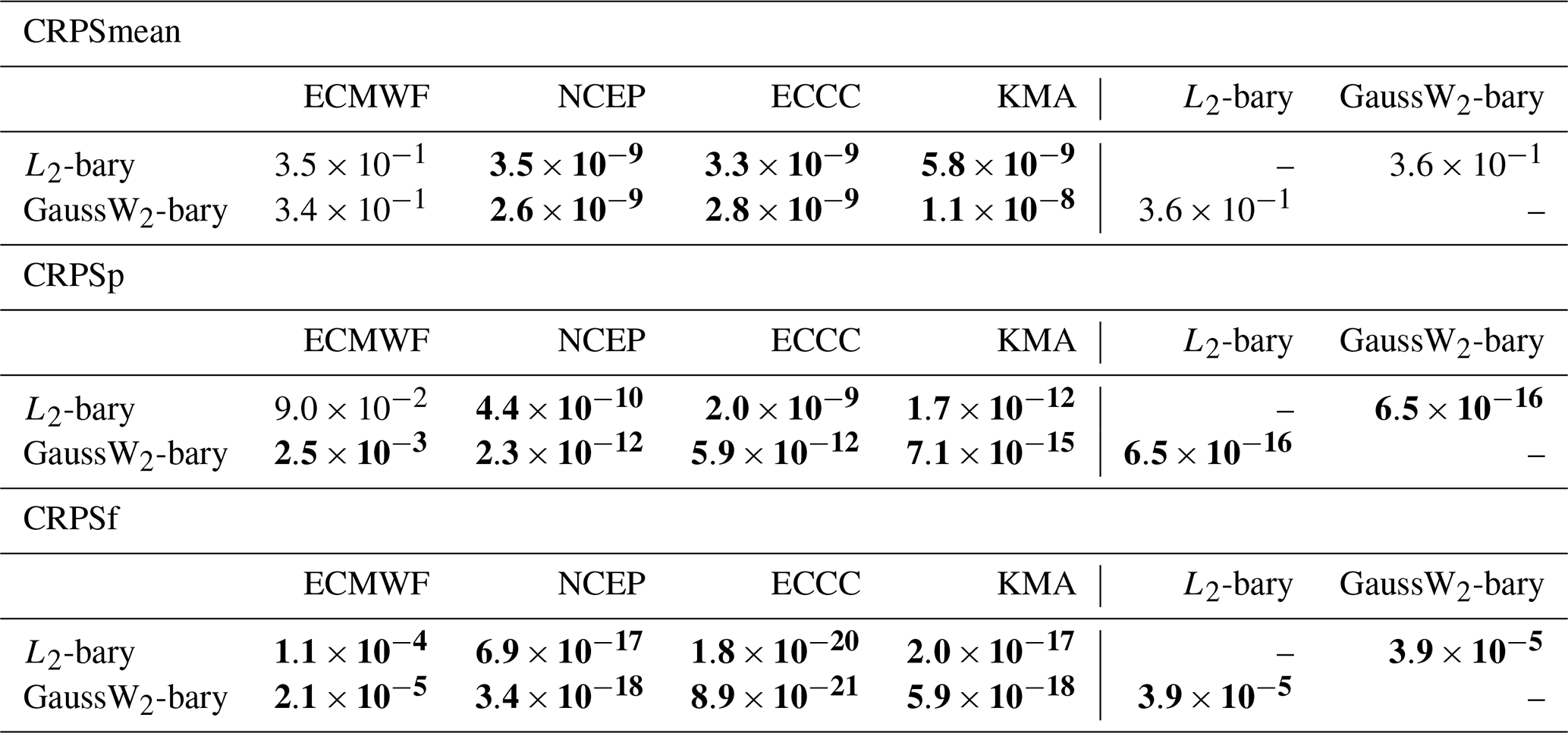
Table D2 Two-sided Wilcoxon test's p-value for the 10 m wind speed (ws10m) for weeks 3 and 4 combined. Bold indicates that the models are significantly different from each other at the 5 % significance level (i.e. p-values < 0.05).

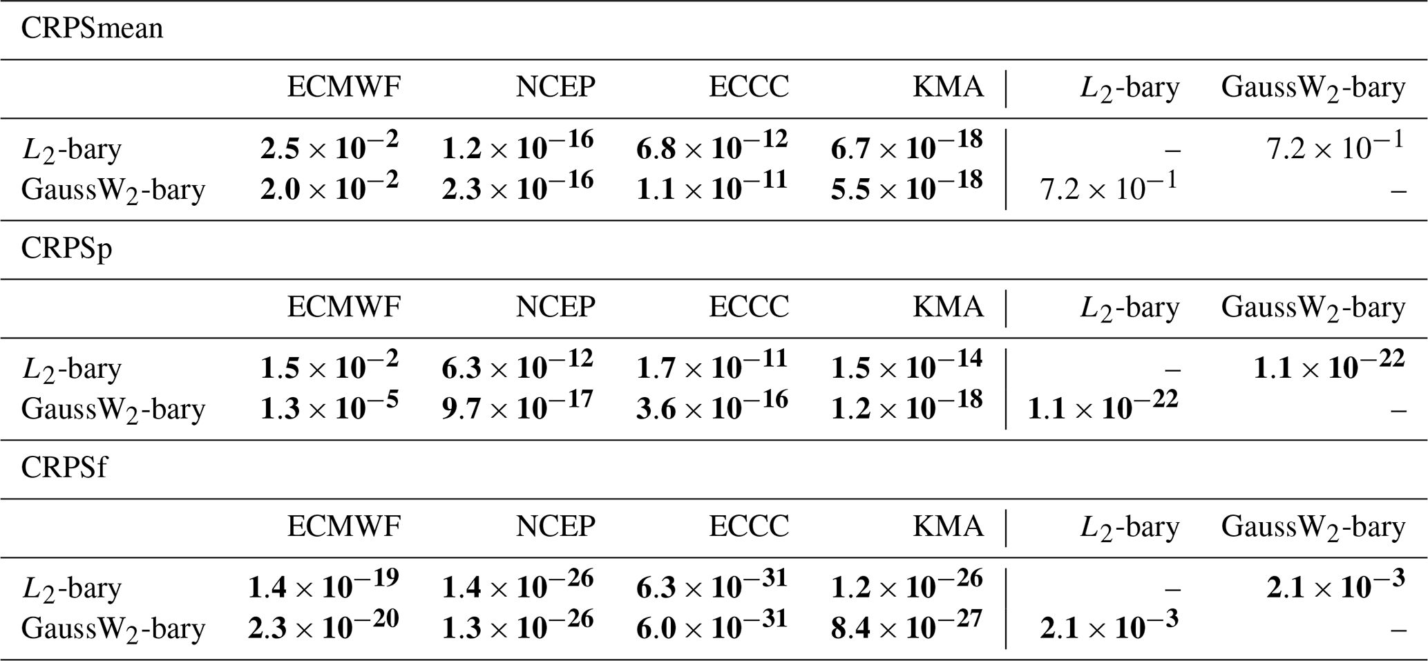
Table D3 Two-sided Wilcoxon test's p-value for the geopotential height (z₅₀₀) for weeks 3 and 4 combined. Bold indicates that the models are significantly different from each other at the 5 % significance level (i.e. p-values < 0.05) with respect to the chosen score.

D2 Barycenters with three models

Table D4 Two-sided Wilcoxon test's p-value for the 2 m temperature (t2m) for weeks 3 and 4 combined. Bold indicates that the models are significantly different from each other at the 5 % significance level (i.e. p-values < 0.05).

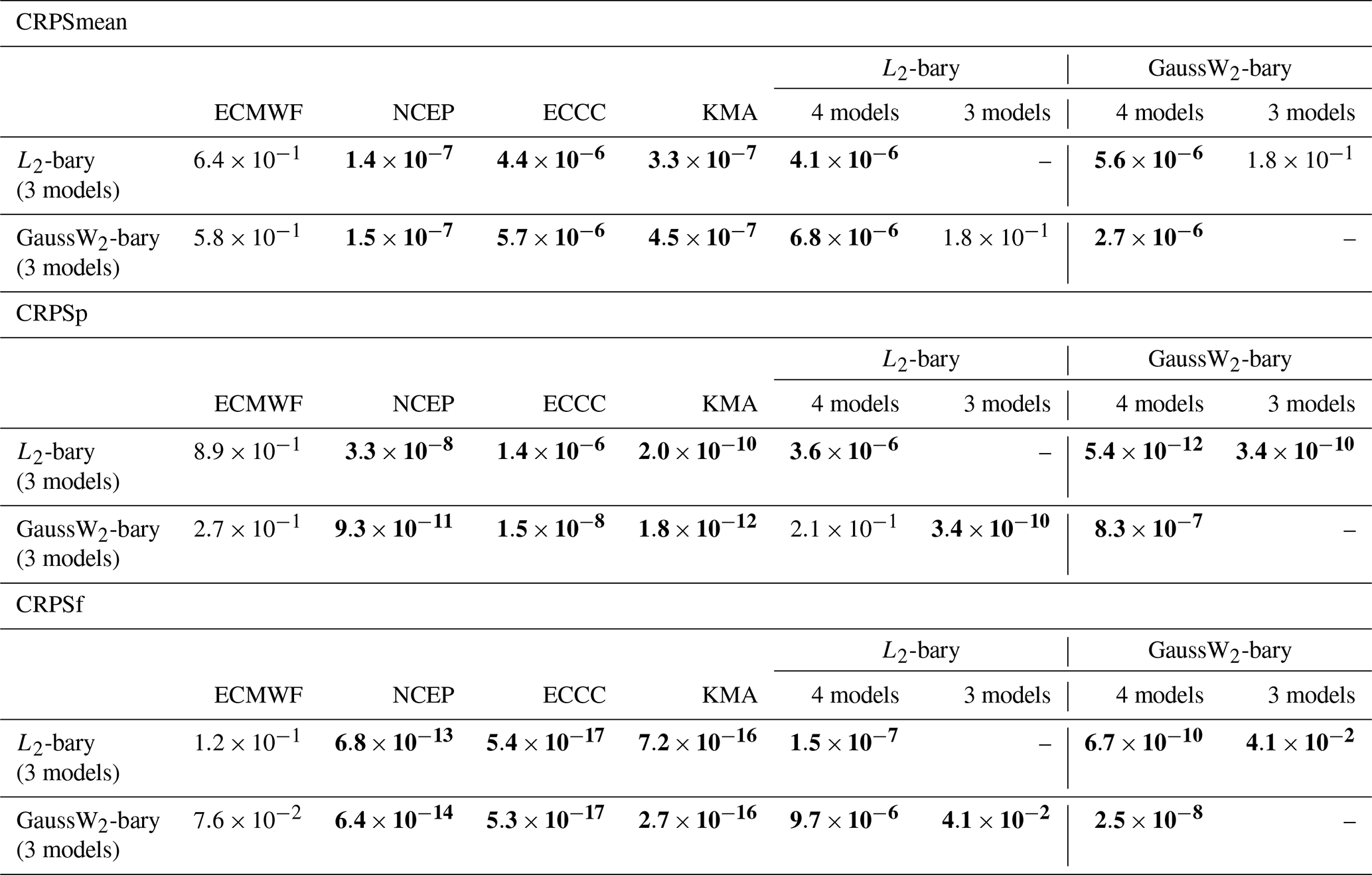
Table D5 Two-sided Wilcoxon test's p-value for the 10 m wind speed (ws10m) for weeks 3 and 4 combined. Bold indicates that the models are significantly different from each other at the 5 % significance level (i.e. p-values < 0.05).

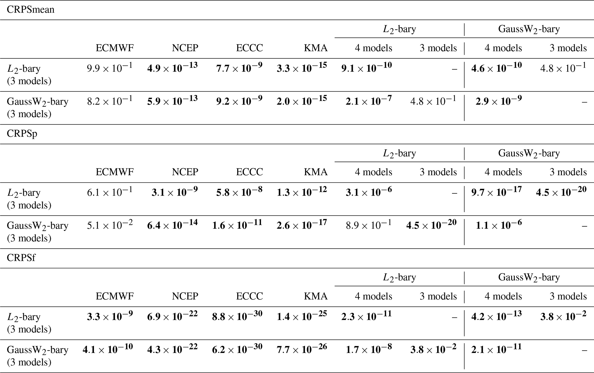
Table D6 Two-sided Wilcoxon test's p-value for the geopotential height (z₅₀₀) for weeks 3 and 4 combined. Bold indicates that the models are significantly different from each other at the 5 % significance level (i.e. p-values < 0.05).