LFD (v1.0): latent-compression-free generative diffusion with geological priors and geophysical regularization for implicit structural modeling

Diffusion models provide a promising way to generate geologically consistent implicit structural models by learning data-driven priors from training examples, potentially improving generalization across surveys. However, existing diffusion transformer pipelines scale poorly to high-dimensional structural modeling data because noise- or velocity-prediction objectives are often unstable at large patch sizes, forcing the use of small patches that lead to long token sequences and high computational cost. To reduce computation, most approaches rely on variational autoencoders (VAEs) and latent diffusion, but robust pretrained VAEs are scarce in geophysics, and enforcing geological priors in latent space is difficult. To address these scalability bottlenecks and the difficulty of enforcing geological priors in latent space, we propose Latent-Compression-Free Generative Diffusion (LFD) with Geological Priors and Geophysical Regularization for implicit structural modeling. Built on flow matching, LFD generates implicit structural models directly in the data space, enabling efficient large-patch Vision Transformer (ViT) inference and allowing fault/horizon constraints and geophysical regularization to be applied explicitly during generation. To strengthen structural conditioning, we design a structure-enhanced transformer that injects horizon and fault embeddings at multiple layers. We further introduce two prior-guided losses: a horizon loss to match the generated models to the input horizons, and a fault-aware bending-energy term that regularizes smoothness while ignoring stencils across faults. By enforcing these priors directly in the data space, the model is effectively constrained to generate geologically reasonable structures. Experiments on both synthetic data and real surveys validate the effectiveness of LFD for prior-guided implicit structural modeling. Benefiting from large-patch inference, LFD generates a 512×512 model in 1.56 s on an NVIDIA H20 GPU. With relative positional encoding, LFD can be extended to higher resolutions via simple adaptation without retraining. Overall, LFD offers new insights into deploying diffusion models for high-dimensional implicit structural modeling problems, enabling efficient generation with interpretable, prior-guided constraints.

1 Introduction

Implicit structural modeling aims to recover a continuous subsurface representation from sparse and heterogeneous geological observations. A common formulation estimates an implicit scalar field, often referred to as the relative geological time (RGT), whose iso-surfaces represent stratigraphic interfaces (Mallet, 1989; Houlding, 1994; Lajaunie et al., 1997). Compared with explicit surface-based representations (Caumon et al., 2009), implicit modeling provides a true volumetric description that enables consistent extraction of multiple geological surfaces and unified enforcement of heterogeneous constraints (Maxelon et al., 2009; Caumon et al., 2013; Pizzella et al., 2022; Arienti et al., 2025). As a result, implicit structural models have increasingly been adopted in a wide range of applications, including geological surveying and mapping (MacCormack et al., 2019; Guo et al., 2018), seismic interpretation (Wu and Hale, 2015; Bi et al., 2021; Wu et al., 2023), joint geophysical inversion and imaging (Zheglova et al., 2018; Giraud et al., 2020, 2024), mineral resource and reserve estimation (Vollgger et al., 2015; Zhong et al., 2019), and stratigraphic-domain transformations for subsequent property modeling (Cowan et al., 2002; Mallet, 2004; Wellmann and Caumon, 2018; de la Varga et al., 2019). Moreover, the automated and efficient nature of implicit modeling facilitates iterative updates and provides a principled basis for incorporating geological knowledge and quantifying structural uncertainty (Wellmann and Caumon, 2018; Yang et al., 2019).

Classical approaches formulate implicit structural modeling as a constrained interpolation or PDE-based problem, incorporating horizons, faults, and orientation information through variational formulations, discretized operators, or least-squares criteria on constraints (Calcagno et al., 2008; Caumon et al., 2013; Grose et al., 2021). To estimate the scalar field from sparse spatial constraints, two major numerical routes are commonly adopted (Renaudeau et al., 2019). The first route uses meshfree global interpolation, including radial basis function interpolation (Cowan et al., 2002; Guo et al., 2018; Zhong et al., 2019) and dual kriging with polynomial drift (Chilès et al., 2007; Calcagno et al., 2008; de la Varga et al., 2019; Pizzella et al., 2022), for which the computational cost is primarily driven by the number of constraint points. The second route relies on grid-based discretization, where the scalar field is computed by discrete smooth interpolation on discontinuity-conforming tetrahedral meshes (Frank, 2007; Caumon et al., 2013; Mallet, 2014; Irakarama et al., 2022; Belhachmi et al., 2025), and the cost is dominated by the mesh resolution. Complementary PDE-based formulations solve for the implicit field by propagating interface and orientation constraints via Hamilton-Jacobi equations (Osher, 1993; Hjelle and Petersen, 2011; Gillberg et al., 2014). Across these formulations, explicit treatment of discontinuities induced by faults and unconformities is a key source of algorithmic and computational complexity. Although these approaches can produce geologically meaningful fields, they can become expensive at high resolution and often require re-solving the system when constraints are updated.

More recently, deep learning has accelerated implicit structural modeling by learning data-driven priors and accelerating inference from sparse geological constraints. Existing approaches can be broadly categorized into two paradigms. The first paradigm is coordinate-based implicit neural representation (Hillier et al., 2021; Li et al., 2025; Fan et al., 2025), where a network takes spatial coordinates as input and outputs the scalar value of the implicit field (Kamath et al., 2026). This is typically realized with fully connected networks. This formulation is highly flexible and can naturally support divide-and-conquer strategies, such as solving separate sub-fields over different stratigraphic or temporal intervals and then assembling them into a globally consistent model (Hillier et al., 2023). The second paradigm is field-based prediction (Wang et al., 2023; Lin et al., 2025), where the input is a structured spatial grid and the network directly maps volumetric observations and constraint rasters to an implicit field, using convolutional networks (Liu and Durlofsky, 2021; Bi et al., 2022; Zhang et al., 2024) or Transformer architectures to capture both local structure and long-range dependencies (Ren et al., 2025). In both paradigms, geological observations and prior rules can be incorporated through differentiable loss terms that constrain the predicted field to honor horizons, faults, and other structural constraints (Wu et al., 2023; Gao and Wellmann, 2025). Despite this progress, generalization across surveys with different structural styles or acquisition characteristics remains challenging, and new areas may still require re-training or fine-tuning (Sheng et al., 2025; Guo et al., 2025).

Generative diffusion models learn data-driven priors by modeling the data distribution rather than memorizing samples (Sohl-Dickstein et al., 2015; Shah et al., 2025; Bonnaire et al., 2025). This distributional learning can improve generalization, which is appealing for implicit structural modeling. Methodologically, diffusion models follow two main routes. Discrete-time Denoising Diffusion Probabilistic Models (DDPMs) define a forward process that gradually corrupts data through many small Gaussian noise increments until it becomes nearly Gaussian, and the reverse model must therefore undo this corruption progressively – removing only a small amount of noise per step to stay close to the target distribution. Consequently, DDPMs generate samples via a multi-step reverse process (Ho et al., 2020; Nichol and Dhariwal, 2021; Choi et al., 2021) and, while conceptually simple, typically require hundreds of sequential denoising steps (i.e., many neural network inferences), making sampling computationally expensive. Continuous-time approaches such as flow matching learn a time-dependent velocity field and sample by integrating an ordinary differential equation (ODE) (Liu et al., 2022; Lipman et al., 2022), often achieving comparable quality with fewer function evaluations and thus better suiting iterative modeling workflows (Dao et al., 2023; Gat et al., 2024). However, deploying flow matching for high-dimensional implicit structural modeling faces key challenges. Diffusion transformers typically rely on VAE-based latent diffusion for efficiency (Rombach et al., 2022; Peebles and Xie, 2023; Lee et al., 2025), yet robust pretrained VAEs are scarce in geophysics. Moreover, geological priors and spatial data are harder to impose and interpret in latent space than in data space (Garayt et al., 2025). Finally, even with a VAE, noise or velocity prediction in the diffusion models makes structural conditioning indirect because most geological constraints are naturally defined on the implicit scalar field (Song et al., 2023). Recent studies suggest that directly predicting the clean sample (denoted as x), instead of regressing noise (ϵ) or velocity (v), can improve optimization and enable large-patch ViT inference (Li and He, 2025). This reduces attention cost and can avoid VAE-based compression, while allowing priors to be imposed directly in data space.

Motivated by these observations, we propose Latent-Compression-Free Generative Diffusion (LFD) with Geological Priors and Geophysical Regularization for implicit structural modeling. Our method is built on three key ideas. First, we adopt an x-prediction formulation that directly predicts the implicit structural models in data space, which makes constraint handling more direct and supports large-patch transformer inference without requiring VAE-based latent compression (Sect. 2.1). Second, we introduce a structure-enhanced network architecture that incorporates interpreted horizons and faults at multiple network layers (Sect. 2.2), enabling these structural constraints to effectively guide the generation of the implicit structural models. Third, we design prior-guided losses derived from geological and geophysical principles to promote structural consistency in the generated models (Sect. 2.3). The trained model can be extended to higher resolutions (e.g., 1024 and 2048) through simple adaptations, even when training is performed at 512 resolution. Extensive experiments on synthetic data and real surveys with complex faulting demonstrate that our approach produces more geologically consistent implicit structural models, offering new insights into applying diffusion-based generative modeling to implicit structural modeling (Sect. 3).

2 Method

This section first reviews the fundamentals of flow-based diffusion models and introduces the x-prediction (denoised-sample prediction) formulation adopted in this work. We then present the denoising Transformer architecture, in which interpreted horizons and faults are injected at multiple network layers to ensure that the generated implicit field remains consistent with the input structural constraints. Finally, to better capture the role of structural conditions in generation and to promote geological consistency, we design two prior-guided losses that explicitly enforce structure-consistent learning.

2.1 x-Prediction Diffusion

We briefly review flow matching (Lipman et al., 2022), a generative diffusion framework that learns a continuous transport from a Gaussian base distribution to the data distribution x∼p_data(x). The base variable is obtained by scaling a standard Gaussian, ϵ=σ ϵ₀ with ${\mathit{ϵ}}_{\mathrm{0}}\sim \mathcal{N}(\mathbf{0},\mathbf{I})$, where the scalar σ>0 is referred to as the noise scale (NS), which scales the amplitude of the Gaussian noise. We construct the noisy sample z_t at a randomly sampled time $t\sim \mathcal{U}(\mathrm{0},\mathrm{1})$ using linear interpolation between the data x and the Gaussian noise ϵ:

$$\begin{array}{}\text{(1)}& {\mathbf{z}}_t=t\mathbf{x}+(\mathrm{1}-t)\mathit{ϵ},\end{array}$$

where z₀=ϵ and z₁=x. Written out, this gives ${\mathbf{z}}_t=t\mathbf{x}+(\mathrm{1}-t)\mathit{\sigma }{\mathit{ϵ}}_{\mathrm{0}}$. The same value of σ is used at training and inference time. Unless stated otherwise, we use σ=0.2 throughout this paper; the motivation for this choice is discussed in Sect. 4. With the linear interpolation path, the target velocity along this path is constant:

$$\begin{array}{}\text{(2)}& \mathbf{v}={\displaystyle \frac{\partial {\mathbf{z}}_t}{\partial t}}=\mathbf{x}-\mathit{ϵ},\end{array}$$

Flow-based methods train a neural network f_θ to estimate the velocity field, denoted by $\widehat{\mathbf{v}}$, where the network takes the time t and the corresponding noisy sample z_t as inputs:

$$\begin{array}{}\text{(3)}& \widehat{\mathbf{v}}=f_{\mathit{\theta }}({\mathbf{z}}_t,t),\end{array}$$

The model is optimized by matching $\widehat{\mathbf{v}}$ to v:

$$\begin{array}{}\text{(4)}& {\mathcal{L}}_{\mathbf{v}}={\mathbb{E}}_{\mathbf{x},\mathit{ϵ},t}\left[{\displaystyle \frac{\mathrm{1}}{N}}{∥\widehat{\mathbf{v}}-\mathbf{v}∥}_{\mathrm{2}}^{\mathrm{2}}\right],\end{array}$$

ℒ_v minimizes the discrepancy between the target velocity field v and its prediction $\widehat{\mathbf{v}}$ via an element-wise mean-squared error over the N pixels of the field, and the expectation is taken over training samples x, Gaussian noise ϵ, and randomly sampled times t. We refer to it as the v-loss.

At inference, we start from a Gaussian sample z₀=σ ϵ₀ at t=0. We then generate a sample by integrating the learned probability-flow ODE from t=0 to t=1. In practice, we discretize the time interval [0,1] into K uniform steps, $\mathit{\{}{t}_k{\mathit{\}}}_{k=\mathrm{0}}^K$, with $t_k=k/K$ (thus $\mathrm{\Delta }t=t_{k+\mathrm{1}}-t_k=\mathrm{1}/K$), and evaluate the network to obtain the velocity field.

$$\begin{array}{}\text{(5)}& {\widehat{\mathbf{v}}}_k=f_{\mathit{\theta }}({\mathbf{z}}_{t_k},t_k),\end{array}$$

An explicit solver updates the state as

$$\begin{array}{}\text{(6)}& {\mathbf{z}}_{t_{k+\mathrm{1}}}={\mathbf{z}}_{t_k}+\mathrm{\Delta }t{\widehat{\mathbf{v}}}_k,\mathrm{\Delta }t=t_{k+\mathrm{1}}-t_k,\end{array}$$

and the final generated sample is obtained at t=1 as $\widehat{\mathbf{x}}\equiv {\mathbf{z}}_{t_K}$. In practice, flow-based sampling typically requires only tens of ODE steps to reach good sample quality (e.g. K=50), which is substantially fewer than the hundreds to thousands of steps often used in DDPM sampling (Zhou et al., 2024).

Learning an accurate velocity field in high-dimensional spaces is challenging for denoisers such as Diffusion Transformers (DiTs) (Peebles and Xie, 2023), often leading to unstable training and reduced sampling efficiency at higher resolutions. As a result, v-prediction models typically use very small square patches (e.g., 2×2, 4×4, or 8×8), which greatly increases token length and attention cost for high-dimensional data (Ma et al., 2024). Most diffusion transformers therefore resort to VAE-based latent diffusion to reduce computation, but this is less appealing for implicit structural models because it may compromise fine structural details and makes it harder to explicitly impose geological priors in the latent space.

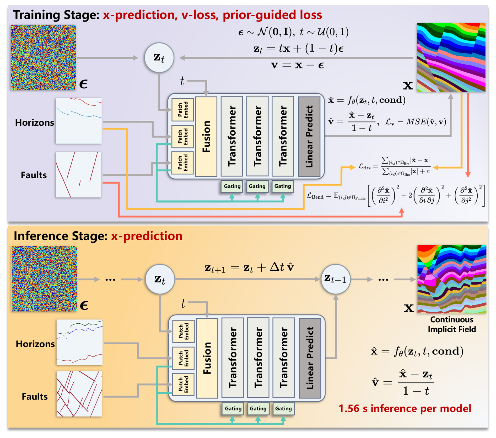
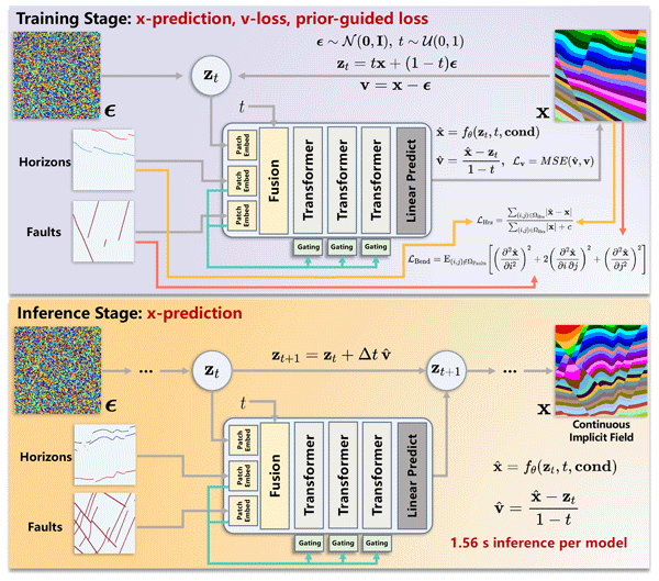
Figure 1 Overview of LFD for implicit structural modeling. Top: Training stage. We sample Gaussian noise ϵ=σϵ₀ with noise scale σ=0.2 and time t, construct ${\mathbf{z}}_t=t\mathbf{x}+(\mathrm{1}-t)\mathit{ϵ}$, and use a structure-enhanced Transformer conditioned on horizons and faults to predict the clean implicit scalar field $\widehat{\mathbf{x}}$. Bottom: Inference stage. Starting from z₀=ϵ, we iteratively integrate the probability-flow ODE using $\widehat{\mathbf{x}}$ to obtain $\widehat{\mathbf{v}}$ and generate the final implicit structural model. Note that the implicit scalar field is a continuous-valued output, the colormap visualizations shown here use discrete color bins solely for display purposes.

In contrast, clean samples usually lie on a lower-dimensional manifold (Chapelle et al., 2009), making it easier and more stable to predict the clean signal directly than to regress the velocity field. Recent studies (Li and He, 2025) have demonstrated that directly predicting the clean data x combined with the v-loss leads to more stable optimization and better sample quality. In this setting, the network no longer predicts the velocity field v; instead, it directly predicts the clean sample $\widehat{\mathbf{x}}$ (as shown in Fig. 1):

$$\begin{array}{}\text{(7)}& \widehat{\mathbf{x}}=f_{\mathit{\theta }}({\mathbf{z}}_t,t,\mathbf{cond}),\end{array}$$

where cond denotes the additional conditioning information. In our implicit structural modeling task, cond specifically represents the input horizons and faults. Consequently, the predicted velocity field $\widehat{\mathbf{v}}$ can be obtained from $\widehat{\mathbf{x}}$ by differentiating the interpolation path in Eq. (1):

$$\begin{array}{}\text{(8)}& \widehat{\mathbf{v}}=\widehat{\mathbf{x}}-{\displaystyle \frac{{\mathbf{z}}_t-t\widehat{\mathbf{x}}}{\mathrm{1}-t}}={\displaystyle \frac{\widehat{\mathbf{x}}-{\mathbf{z}}_t}{\mathrm{1}-t}}\end{array}$$

Based on Eq. (2), we can still compute the v-loss in Eq. (4) for this velocity estimate. This is the x-prediction diffusion formulation adopted in this work. We next introduce the denoising network used in this diffusion framework, which further strengthens structural guidance through explicit conditioning.

2.2 Structure-Enhanced Denoising Transformer

We adopt a standard Vision Transformer (ViT) backbone as the denoising network f_θ (Peebles and Xie, 2023). Since predicting a clean sample on a low-dimensional data manifold is generally easier than regressing the velocity field (Karras et al., 2022), larger patch sizes can be used without sacrificing training stability. In this work, we employ ViT-Base/32 as the backbone, which provides a good trade-off between generation quality and efficiency.

Let P=32 be the patch size and $N=\left(\frac{H}{P}\right)\times \left(\frac{W}{P}\right)$ the number of patches. We tokenize z_t into a sequence of patch tokens using a bottleneck patch embedding (Alemi et al., 2016), which helps stabilize training:

$$\begin{array}{}\text{(9)}& \begin{array}{rl}& {\mathbf{z}}_{\mathbf{x}}={\mathit{\varphi }}_{\mathbf{x}}\left({\mathbf{z}}_t\right)\in {\mathbb{R}}^{N\times d},\\ & {\mathit{\varphi }}_{\mathbf{x}}(\cdot )={\mathrm{Conv}}_{\mathrm{1}\times \mathrm{1}}\left({\mathrm{Conv}}_{P\times P}\right(\cdot \left)\right),\end{array}\end{array}$$

where Conv_P×P denotes a 2D convolution with kernel size P×P and stride P (thus extracting non-overlapping patch features), and Conv_1×1 denotes a 1×1 convolution that linearly projects the bottleneck features to the ViT hidden dimension d.

We encode horizons and faults using two separate bottleneck embedding modules. Denote the horizon input by h and the fault input by f. Their token embeddings are

$$\begin{array}{}\text{(10)}& {\mathbf{z}}_{\mathbf{h}}={\mathit{\varphi }}_{\mathbf{h}}\left(\mathbf{h}\right),{\mathbf{z}}_{\mathbf{f}}={\mathit{\varphi }}_{\mathbf{f}}\left(\mathbf{f}\right),\end{array}$$

where ϕ_h(⋅) and ϕ_f(⋅) have the same bottleneck architecture as ϕ_x(⋅) but are parameterized independently. For positional encoding of ViTs, we use sine–cosine embeddings to provide a stable global reference and rotary position embedding (RoPE) (Su et al., 2024) to improve relative position modeling, which improves generalization to varying input sizes (Heo et al., 2024).

We fuse the noisy tokens with structural tokens by element-wise addition, a common token-fusion strategy in Transformers that combines multiple embeddings while keeping the token dimension and sequence length unchanged (Peebles and Xie, 2023):

$$\begin{array}{}\text{(11)}& {\mathbf{z}}^{\left(\mathrm{0}\right)}={\mathbf{z}}_{\mathbf{x}}+{\mathbf{z}}_{\mathbf{h}}+{\mathbf{z}}_{\mathbf{f}},\end{array}$$

where ${\mathbf{z}}^{\left(\mathrm{0}\right)}\in {\mathbb{R}}^{N\times d}$ denotes the fused token sequence at the input of the Transformer.

Beyond the input-level fusion, we further strengthen structural guidance by injecting horizon and fault embeddings into each Transformer layer as residual priors. Specifically, given the intermediate tokens z^(ℓ), we form a structure-enhanced representation by

$$\begin{array}{}\text{(12)}& {\stackrel{\mathrm{̃}}{\mathbf{z}}}^{\left(\mathrm{\ell }\right)}={\mathbf{z}}^{\left(\mathrm{\ell }\right)}+{\mathit{\alpha }}_{\mathrm{\ell }}{\mathbf{z}}_{\mathbf{h}}+{\mathit{\beta }}_{\mathrm{\ell }}{\mathbf{z}}_{\mathbf{f}},\end{array}$$

where α_ℓ and β_ℓ are learnable, layer-adaptive weights that control how strongly each layer uses horizon and fault priors. Finally, we obtain $\widehat{\mathbf{x}}$ using Eq. (7) with $\mathbf{cond}=(\mathbf{h},\mathbf{f})$, where the residual injections encourage structure-consistent denoising across layers.

To further strengthen the role of the input structural constraints in guiding generation, we next introduce prior-guided loss terms designed directly in the data space.

2.3 Prior-Guided Losses

As the model directly predicts the clean data $\widehat{\mathbf{x}}$, geological observations and prior constraints can be imposed in a straightforward and differentiable manner. We introduce two prior-guided terms, a horizon loss ℒ_Hrz and a fault-aware bending-energy regularizer ℒ_Bend, to enforce consistency with the input horizons while promoting smoothness within stratigraphic blocks without smoothing across faults.

The implicit structural model is required to align with the input horizons. Let ${\mathbf{M}}_{\mathbf{h}}\in \mathit{\{}\mathrm{0},\mathrm{1}{\mathit{\}}}^{H\times W}$ be a binary mask derived from the input horizon data, indicating horizon locations. We penalize deviations on the horizon by the mean absolute error normalized by the summed target magnitude:

$$\begin{array}{}\text{(13)}& {\mathcal{L}}_{\mathrm{Hrz}}={\displaystyle \frac{{∥{\mathbf{M}}_{\mathbf{h}}\odot \left(\widehat{\mathbf{x}}-\mathbf{x}\right)∥}_{\mathrm{1}}}{{∥{\mathbf{M}}_{\mathbf{h}}\odot \mathbf{x}∥}_{\mathrm{1}}+c}},\end{array}$$

where ⊙ denotes element-wise multiplication and c is a small constant. This normalization reduces sensitivity to the absolute scale of implicit structural model values.

Additionally, implicit structural models are expected to form a globally smooth field, and horizons should not exhibit excessive curvature in a geologically reasonable interpretation. We therefore introduce a bending-energy regularizer (Renaudeau et al., 2019; Belhachmi et al., 2025) that penalizes second-order variations of the predicted implicit scalar field. Importantly, this smoothness prior should not be enforced across faults, since faults correspond to discontinuities. To honour fault discontinuities, we compute the bending energy only on the non-fault region and use fault-aware finite-difference stencils that do not cross fault pixels.

Let ${\mathbf{M}}_{\mathbf{f}}\in \mathit{\{}\mathrm{0},\mathrm{1}{\mathit{\}}}^{H\times W}$ denote the input fault mask, and define the fault domain ${\mathrm{\Omega }}_{\mathrm{Faults}}=\mathit{\left\{}\right(i,j\left)\right|{\mathbf{M}}_{\mathbf{f}}(i,j)=\mathrm{1}\mathit{\}}$. The fault-aware bending-energy loss is defined as

$$\begin{array}{}\text{(14)}& \begin{array}{rl}{\mathcal{L}}_{\mathrm{Bend}}=& {\mathrm{E}}_{(i,j)\notin {\mathrm{\Omega }}_{\mathrm{Faults}}}\left[{\left({\displaystyle \frac{\mathrm{1}}{\mathrm{\Delta }{i}^{\mathrm{2}}}}{\displaystyle \frac{{\partial }^{\mathrm{2}}\widehat{\mathbf{x}}}{\partial i^{\mathrm{2}}}}\right)}^{\mathrm{2}}\right.\\ & \left.+\mathrm{2}{\left({\displaystyle \frac{\mathrm{1}}{\mathrm{\Delta }i\mathrm{\Delta }j}}{\displaystyle \frac{{\partial }^{\mathrm{2}}\widehat{\mathbf{x}}}{\partial i\partial j}}\right)}^{\mathrm{2}}+{\left({\displaystyle \frac{\mathrm{1}}{\mathrm{\Delta }{j}^{\mathrm{2}}}}{\displaystyle \frac{{\partial }^{\mathrm{2}}\widehat{\mathbf{x}}}{\partial j^{\mathrm{2}}}}\right)}^{\mathrm{2}}\right],\end{array}\end{array}$$

where Δi and Δj denote the grid spacing in the i- and j-directions, respectively, and the second-order derivatives are implemented with fault-aware discrete operators that ignore stencils crossing fault pixels. Specifically, for each second-order derivative term, we adopt a stencil-validity masking strategy: the curvature contribution at a given location is computed only if all sampling points involved in the corresponding standard central-difference stencil lie in the non-fault region; if any point of the stencil falls on a fault pixel, the curvature term at that location is set to zero rather than being approximated with a lower-order one-sided or truncated scheme. As a result, the accuracy of the stencil itself does not vary near fault boundaries. The final training objective combines the flow matching loss with the prior-guided losses:

$$\begin{array}{}\text{(15)}& \mathcal{L}={\mathcal{L}}_{\mathbf{v}}+{\mathit{\lambda }}_{\mathrm{Hrz}}{\mathcal{L}}_{\mathrm{Hrz}}+{\mathit{\lambda }}_{\mathrm{Bend}}{\mathcal{L}}_{\mathrm{Bend}},\end{array}$$

where λ_Hrz and λ_Bend are weighting factors used to balance the relative magnitudes of different loss terms during training. In practice, we set λ_Hrz=10 and λ_Bend=0.1 to keep ℒ_v, ℒ_Hrz, and ℒ_Bend on comparable scales throughout training, thereby avoiding any single term dominating the gradients and ensuring stable optimization.

These design choices define the overall LFD framework, combining x-prediction with the v-loss, structure-enhanced denoising transformers, and data-space prior-guided regularization. In the following, we evaluate its effectiveness on synthetic data and challenging field examples.

3 Experiments

3.1 Data Preparation

To train and validate our conditional generative diffusion model for implicit structural modeling, we construct a large synthetic dataset in two stages: (i) geology-informed 3D structural simulation and (ii) conversion to 2D conditional training pairs (as shown in Fig. 2).

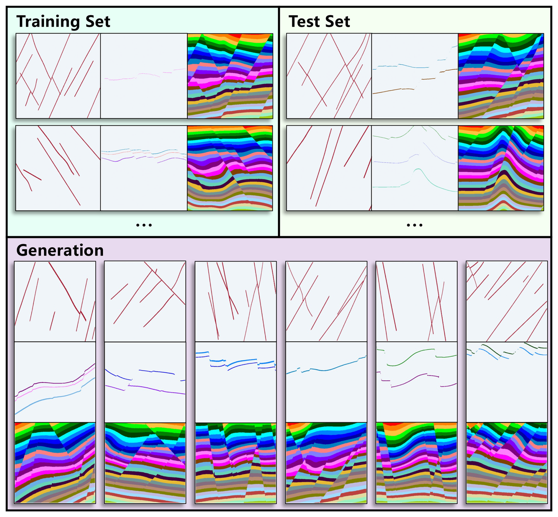
Figure 2 Synthetic dataset examples used for training, testing, and conditional generation. Top: representative samples from the training set (left) and test set (right). Bottom: conditional generations from LFD.

First, we generate realistic 3D implicit structural models using a simulation workflow in the spirit of Wu et al. (2020). Folding deformation is created by superposing multiple parameterized Gaussian functions, with key parameters randomly sampled to cover a wide range of fold wavelengths, amplitudes, and asymmetries. We then introduce geologically plausible faulting by constructing 3D fault surfaces, assembling fault networks (fault assemblages), and simulating 3D slip distributions between the hanging wall and footwall. Building on the resulting folded–faulted framework, we further incorporate unconformities and associated stratal termination patterns (e.g., onlap, downlap, toplap, and related terminations). This procedure yields 3000 realistic 3D implicit structural models at $\mathrm{512}\times \mathrm{512}\times \mathrm{512}$ resolution, each paired with a full-volume 3D fault mask. The combination of explicit fold/fault/unconformity rules and controlled parameter randomization ensures both geological plausibility and broad structural–stratigraphic diversity across the dataset. It should be noted that the synthetic dataset is generated through a geometry-based structural simulation workflow rather than an explicit reconstruction of geological event histories. This design prioritizes structural diversity for diffusion-model training rather than reproducing specific geological evolution pathways.

Second, to match our 2D conditional diffusion training setup, we randomly extract 512×512 slices from the 3D volumes of implicit models and fault masks along both inline and crossline directions to increase directional variability and improve generalization. From each 2D implicit model (used as the target label (x)), we derive conditioning inputs in two forms: (1) the corresponding full 2D fault mask (f), providing complete fault-boundary conditions, and (2) sparse horizon constraints (h) obtained by randomly selecting between 1 and 6 relative geological time (RGT) values and extracting the corresponding iso-contours from the target implicit structural model. This strategy mimics practical interpretation scenarios where only a limited number of horizons are available as constraints (following Bi et al., 2022). These complementary conditions – global fault geometry from (f) and sparse stratigraphic cues from (h) – jointly guide the conditional diffusion model to generate structurally consistent implicit scalar fields. In total, we construct 64 000 training pairs $\mathit{\left\{}\right(\mathbf{h},\mathbf{f}),\mathbf{x}\mathit{\}}$, and normalize both inputs and target implicit fields to $[-\mathrm{1},\mathrm{1}]$ to stabilize training. Throughout this paper, we visualize the continuous implicit scalar field using a discrete colormap to better reveal the stratigraphic layering.

For field-data evaluation, we test on several real-survey cases from Huang and Liu (2017), characterized by complex flower-structure faulting with associated horizon interpretations, as shown in the first two columns of Fig. 3. We denote the five cases in Fig. 3a–e as real-1 through real-5, respectively. Since implicit scalar field values on horizons are unavailable in real surveys, we assign normalized horizon values by mapping the mean horizon depth ratio linearly to $[-\mathrm{1},\mathrm{1}]$, providing a consistent relative ordering of horizons for conditioning.

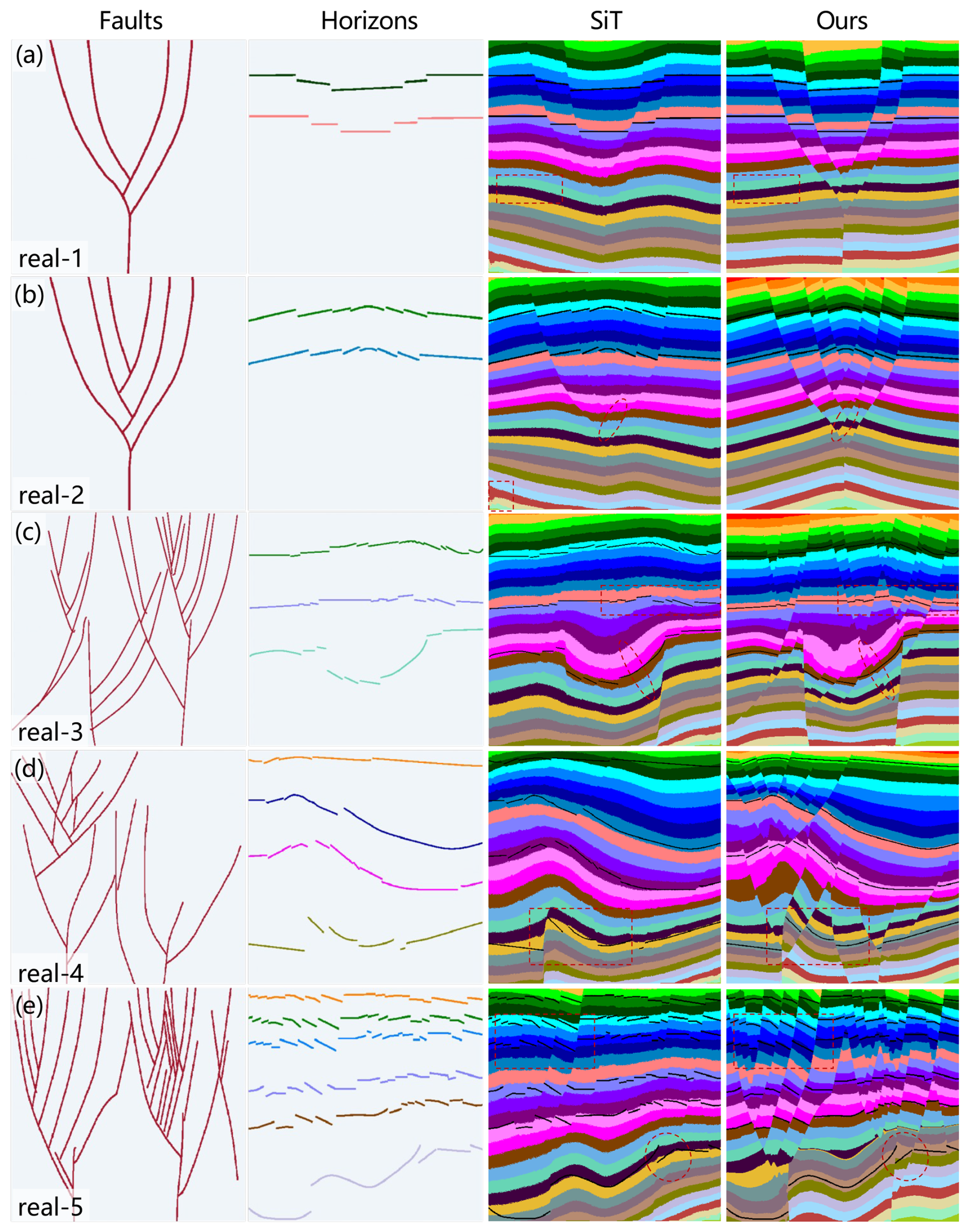
Figure 3 Field data results on flower-structure faulting. (a–e) Five real-survey examples with progressively increasing structural complexity from Huang and Liu (2017). From left to right, each row shows the input fault interpretation, the input horizon constraints, the implicit structural model generated by SiT, and the result produced by our method.

3.2 Training Settings

We initialize the ViT-Base/32 backbone with pretrained weights from Li and He (2025). We set the noise scale to 0.2 when constructing noisy samples during training, because it yields smoother implicit fields in our experiments. We discuss the impact of noise scale in Sect. 4. We use a learning rate of $\mathrm{5}\times {\mathrm{10}}^{-\mathrm{5}}$ with a batch size of 128 and train for 600 epochs. Training is performed on three 96 GB NVIDIA H20 GPUs and takes approximately 18 h. At inference, we discretize the ODE integration into K=50 steps for all experiments.

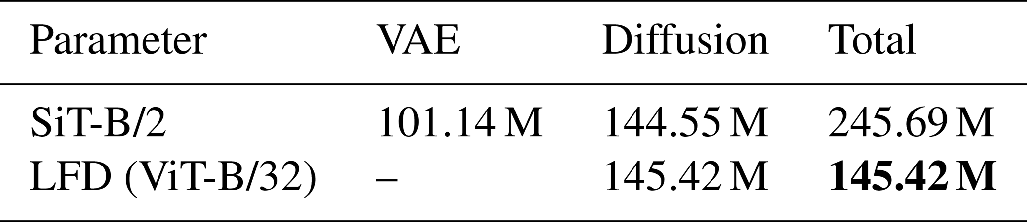
For comparison, we implement a latent-diffusion baseline that follows the SiT (Ma et al., 2024) training paradigm with a pretrained VAE (Rombach et al., 2022). As reported in Table 1, our model (LFD) and the SiT baseline have comparable parameter counts, making the comparison fair. All models are trained under the same settings as above.

Table 1 Model parameter counts. Bold indicates the smallest total parameter count.

3.3 Evaluation Metric

To quantify horizon adherence on real surveys, where ground-truth implicit structural models are unavailable, we propose the Horizon Consistency Error (HCE), which measures how consistent the predicted implicit field values are along each input horizon. Let $\widehat{\mathbf{x}}\in {\mathbb{R}}^{H\times W}$ denote the generated implicit model, and let $\mathbf{H}\in \mathit{\{}\mathrm{0},\mathrm{1},\mathrm{\dots }{\mathit{\}}}^{H\times W}$ be the horizon label map, where $\mathbf{H}(i,j)=\mathrm{0}$ indicates background and $\mathbf{H}(i,j)=k$ denotes the kth horizon. For each horizon $k\in \mathcal{K}=\mathit{\left\{}k\right|k\ne \mathrm{0}\mathit{\}}$, we define the horizon support

$$\begin{array}{}\text{(16)}& {\mathrm{\Omega }}_k=\mathit{\left\{}\right(i,j\left)\right|\mathbf{H}(i,j)=k\mathit{\}}.\end{array}$$

We first compute the mean implicit value on that horizon,

$$\begin{array}{}\text{(17)}& {\mathit{\mu }}_k={\displaystyle \frac{\mathrm{1}}{\left|{\mathrm{\Omega }}_k\right|}}\sum _{(i,j)\in {\mathrm{\Omega }}_k}\widehat{\mathbf{x}}(i,j),\end{array}$$

and then measure the mean absolute deviation from this mean:

$$\begin{array}{}\text{(18)}& e_k={\displaystyle \frac{\mathrm{1}}{\left|{\mathrm{\Omega }}_k\right|}}\sum _{(i,j)\in {\mathrm{\Omega }}_k}\left|\widehat{\mathbf{x}}(i,j)-{\mathit{\mu }}_k\right|.\end{array}$$

If the generated implicit field is well aligned with the kth horizon, $\widehat{\mathbf{x}}$ should be nearly constant along Ω_k, yielding e_k≈0; otherwise, e_k increases as $\widehat{\mathbf{x}}$ varies along the horizon. Finally, we aggregate the per-horizon errors using a pixel-wise normalized average:

$$\begin{array}{}\text{(19)}& {\mathcal{M}}_{\mathrm{HCE}}={\displaystyle \frac{{\sum }_k\left|{\mathrm{\Omega }}_k\right|e_k}{{\sum }_k\left|{\mathrm{\Omega }}_k\right|}}.\end{array}$$

This pixel-wise normalized aggregation avoids dependence on the number and length of horizons, enabling fair comparisons across cases.

3.4 Results

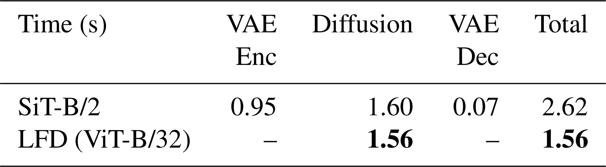
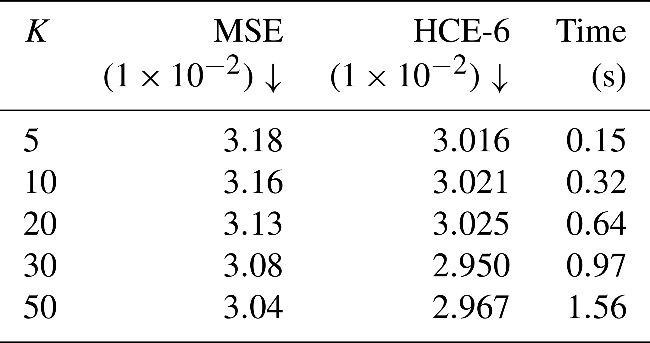
Figure 2 shows representative synthetic test examples. The generated implicit models honor the input faults and horizons and produce sharp, fault-aligned discontinuities. This indicates that the structural constraints are effectively enforced during generation. By default, all results in this paper are generated using K=50 ODE sampling steps. Benefiting from large-patch inference, generating a 512×512 implicit model under this setting requires only 1.56 s on a single NVIDIA H20 GPU (see Sect. 4 for a sensitivity analysis on the number of sampling steps). This runtime is measured with batch size 1 by generating 20 samples and reporting the average per-sample time. As summarized in Table 2, our method is faster than the SiT baseline, largely because the larger patch size reduces token length and attention cost. Moreover, SiT additionally incurs VAE encoding and decoding overhead, further widening the efficiency gap.

Table 2 Inference times. Bold indicates the shortest inference time.

We further evaluate the method on five challenging real-survey cases with complex flower-structure faulting (Fig. 3). As shown in Fig. 3a–e, the structural complexity increases progressively from real-1 to real-5, placing higher demands on both fault continuity and horizon conformity. The SiT baseline (third column in Fig. 3) can recover the major faults, but without explicit geological priors its generated implicit models tend to drift away from the input horizons, which in turn degrades finer-scale stratigraphic features.

Beyond this overall trend, the visual comparisons in Fig. 3 highlight several characteristic behaviors. In Fig. 3a, the red box shows that SiT exhibits noticeably stronger noise than our method, which may be related to the sensitivity of VAE decoding to latent perturbations that can be amplified into artifacts in the implicit field (Liu et al., 2026). In Fig. 3b, the red box reveals anomalous values in the SiT result, indicating potential instabilities in latent-space generation. Moreover, the red ellipse indicates that our method can still enforce a fault-aligned discontinuity in the implicit field even where horizon constraints are sparse, whereas SiT fails to express the fault geometry at that location. In Fig. 3d and e, the red boxes further demonstrate that our method remains better anchored to the input horizons and produces sharper, more clearly delineated fault boundaries. We also note a challenging region in Fig. 3e (red ellipse), where both methods deviate from the input horizons due to the presence of pronounced thrusting, making faithful recovery particularly difficult. This represents a limitation of our current approach; nevertheless, our method still achieves relatively improved horizon conformity compared with SiT in this setting.

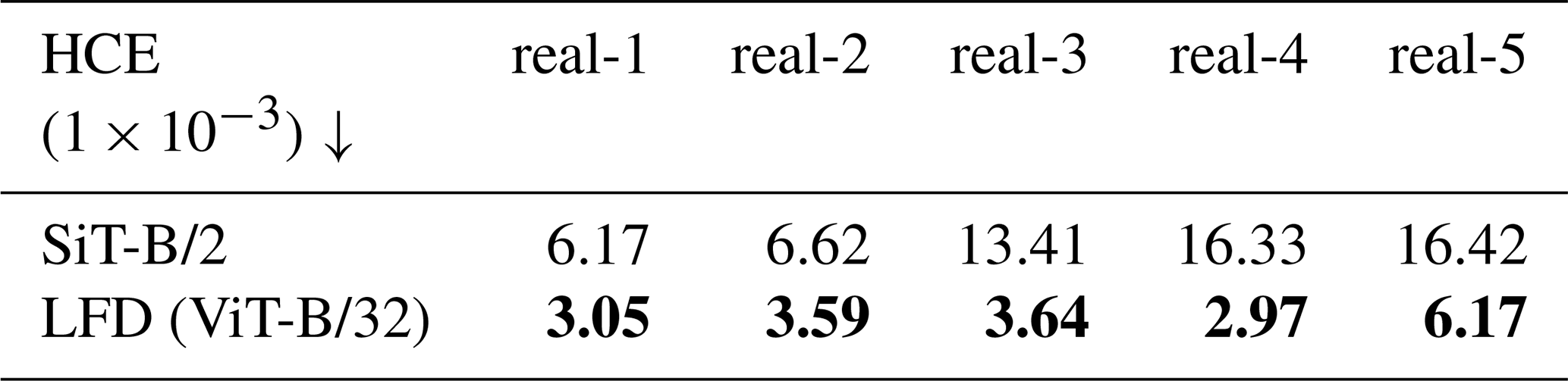
The above visual comparisons are quantitatively confirmed by the error metrics given in Table 3, which show that our approach achieves better horizon consistency than SiT, consistent with Fig. 3 and highlighting the value of explicitly injecting geological priors for reliable implicit structural modeling in complex real surveys.

Table 3 Values of Horizon Consistency Error (HCE) on field data shown in Fig. 3. Bold indicates the lowest HCE value for each case.

3.5 Ablation Study on Uncertainty: Effects of Conditioning Sparsity and Prior-Guided Regularization Strength

To investigate how the number of input horizon constraints affects generation quality and realization variability, we conduct an ablation study in which the number of input horizons is systematically reduced from 6 to 4, 2, and 1 (top row in Fig. 4). For each configuration, we generate 20 independent realizations by sampling different initial Gaussian noise fields while keeping the fault and horizon conditioning fixed, and compute the pixel-wise variance across realizations to quantify uncertainty.

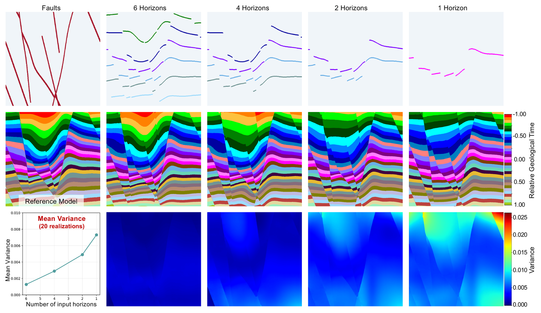
Figure 4 Ablation study on horizon sparsity and realization uncertainty. Top row: input conditioning, showing the shared fault interpretation (leftmost) and horizon inputs with 6, 4, 2, and 1 horizons. Middle row: mean implicit structural model over 20 realizations for each horizon configuration, with the reference model shown in the leftmost panel. Bottom row: pixel-wise variance across 20 realizations (leftmost panel: mean variance as a function of the number of input horizons), demonstrating that realization variance increases monotonically as horizon constraints become sparser.

The middle row of Fig. 4 shows the mean implicit structural models over 20 realizations generated under each sparsity level. As the number of input horizons decreases, the generated models remain geologically plausible but exhibit increasing variability in stratigraphic geometry, particularly in regions far from the remaining horizon constraints. This reflects the model's learned prior filling in the unconstrained space with a broader range of geologically consistent solutions. We note that, since these 20 realizations are generated from different initial noise samples, this also indicates that the sampled initial noise has a visible influence on the resulting structural details, with different noise samples leading to different specific realizations, while the overall outputs remain geologically plausible.

The bottom row of Fig. 4 shows the spatial distribution of pixel-wise variance across 20 realizations for each horizon configuration. With 6 input horizons, variance is uniformly low across the model domain, indicating that dense conditioning effectively anchors the generation. As the number of horizons is reduced to 4, 2, and finally 1, high-variance regions progressively expand, concentrating first in areas between horizons and eventually spanning the majority of the model domain. This spatial pattern is consistent with the intuition that uncertainty grows where conditioning data are absent. The mean variance plot (bottom-left panel of Fig. 4) further confirms this trend quantitatively: mean variance increases monotonically from approximately 0.0013 (6 horizons) to 0.0073 (1 horizon), demonstrating that realization spread is directly controlled by the density of horizon constraints. Collectively, these results suggest that LFD generates a data-consistent distribution: when conditioning data are abundant, the model converges to consistent solutions; when data are sparse, the model appropriately broadens its output distribution to reflect the increased geological ambiguity, rather than collapsing to a single overconfident prediction.

Beyond conditioning sparsity, we further investigate how the strength of the proposed fault-aware bending-energy regularization affects the realization ensemble. For each bending-energy weight ${\mathit{\lambda }}_{\mathrm{Bend}}\in \mathit{\{}\mathrm{0},\mathrm{0.1},\mathrm{1}\mathit{\}}$ (λ_Bend=0.1 being the default used throughout this paper), we train a separate model under the same training settings and evaluate it on the full validation set (3200 cases). For each case, we extract the central horizon of the implicit field together with the corresponding fault mask as the conditioning input, and generate 20 realizations from different noise seeds. We report the resulting pixel-wise Mean Squared Error (MSE), the Horizon Consistency Error (HCE-6, evaluated on 6 horizons uniformly extracted from the ground-truth implicit field), and the mean realization variance, averaged over the validation set, in Table 4.

Table 4 Ablation on fault-aware bending-energy weight λ_Bend.

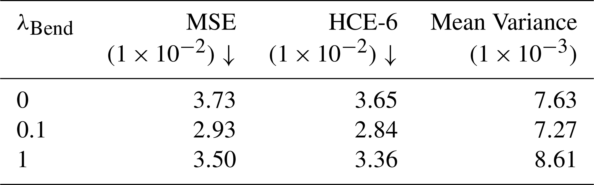
As shown in Table 4, MSE and HCE-6 do not vary monotonically with λ_Bend, but both are consistently lower with the bending-energy prior enabled than without it, indicating that the regularization yields realizations that are more stable and closer to the reference model, rather than drifting into implausible solutions. In particular, λ_Bend=0.1 achieves the lowest pixel-wise error among the three settings. At the same time, the prior does not reduce realization variance; the strongest setting (λ_Bend=1) yields the highest variance among the three, showing that this improved stability does not come at the cost of the model's ability to represent structural uncertainty.

4 Discussion

In developing LFD, we observed several interesting behaviors that provide additional insight into diffusion-based implicit structural modeling, while also revealing practical limitations of the current study. We summarize these findings below.

Resolution robustness. Our model is trained on 512×512 samples, yet we observe encouraging robustness to higher resolutions. In principle, the same adaptation applies to other larger input sizes; here we use 1024×1024 and 2048×2048 as representative examples. In testing, we upsample the input horizons and faults to 1024×1024 and 2048×2048 using nearest-neighbor interpolation. To keep the token length unchanged (i.e., a 16×16 token grid), we increase the patch size to P=64 and P=128 for 1024 and 2048 inputs, respectively. For each bottleneck patch embedding module, the spatial grid changes with resolution; therefore, we interpolate the positional embeddings and reuse the pretrained network parameters accordingly to adapt the model to the new grid. Surprisingly, the generated implicit models remain high-quality at both 1024 and 2048 resolutions (Fig. 5). We attribute this behavior partly to the relative positional encoding (RoPE), which provides a degree of resolution robustness by expressing positions in a scale-consistent manner. This observation is consistent with prior findings that RoPE improves resolution extrapolation in vision transformers (Heo et al., 2024; van de Geijn et al., 2025). We note, however, that this finding may be task-dependent: implicit structural models are typically smooth fields and do not require extremely high-frequency details.

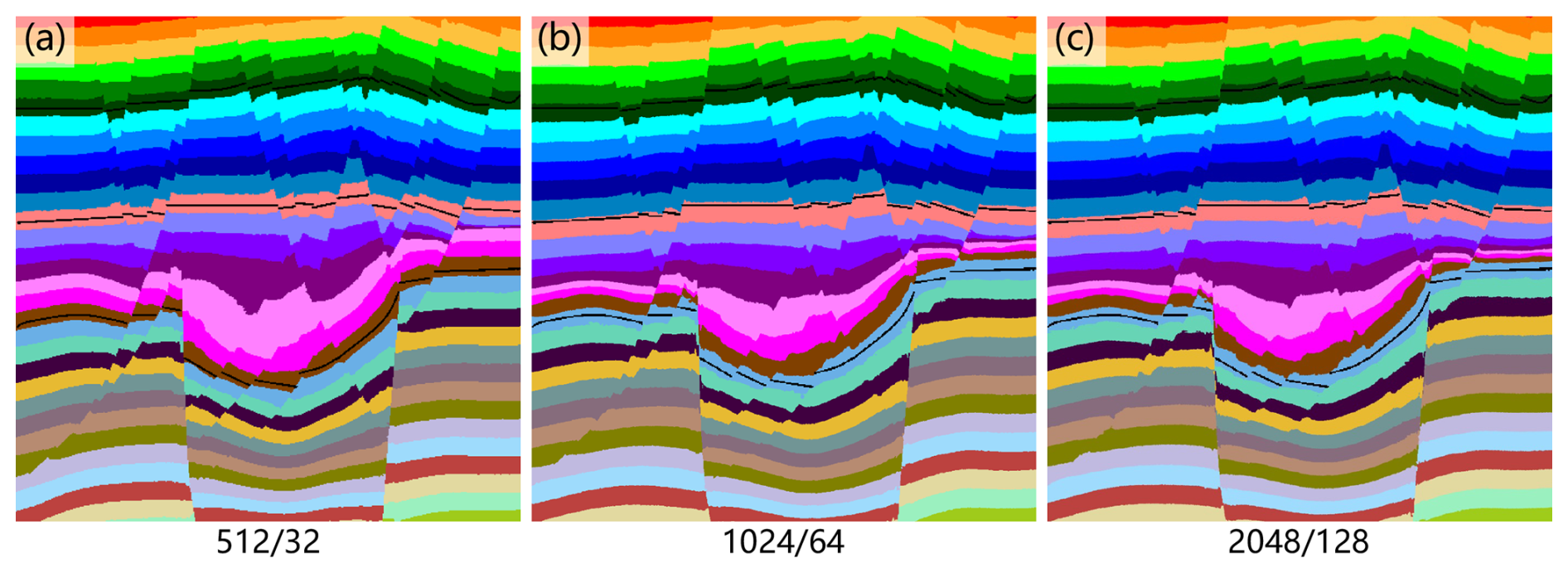
Figure 5 Resolution generalization. The model trained at 512×512 is directly applied to higher resolutions by adjusting the patch size to keep the token grid fixed. From left to right: 512/32 (same result as the real-3 case in Fig. 3c), 1024/64, and 2048/128 (resolution/patch size). The model preserves high-quality implicit structural predictions at 1024×1024 and 2048×2048 without additional training.

Impact of noise scale. We find that the noise scale is a critical factor for implicit structural modeling. In early experiments, using commonly adopted noise scales for natural-image diffusion (e.g., 1.0 or 2.0) often led to overly noisy generations even with prolonged training. This is likely because implicit structural models exhibit relatively smooth distributions, for which excessively strong corruption can hinder stable denoising. To probe this behavior before committing to a full retraining, we took the exploratory model trained with NS=2.0 and varied only the inference-time noise scale (Fig. 6), and observed that decreasing it yields noticeably smoother and more geologically reasonable implicit fields. On the basis of this observation we retrained the model with NS=0.2, which is used for all other results in this paper. This finding provides practical guidance for deploying diffusion models in geophysics: the noise scale should be tuned to the target task and data characteristics to achieve optimal generation quality.

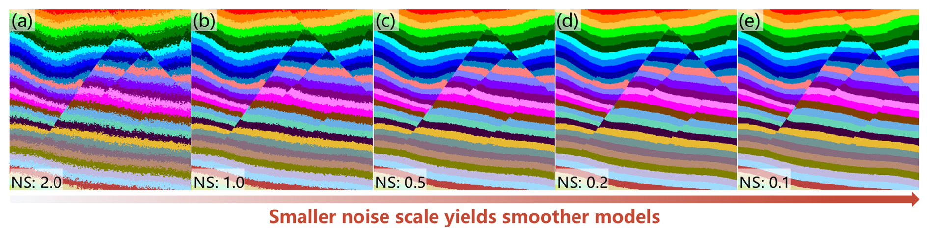
Figure 6 Effect of noise scale (NS) on generation. This experiment was carried out with an early exploratory model trained with NS=2.0, before the final configuration was fixed. During inference, we vary only the noise scale while keeping all other settings fixed. Panels (a)–(e) correspond to $\mathrm{NS}=\mathit{\{}\mathrm{2.0},\mathrm{1.0},\mathrm{0.5},\mathrm{0.2},\mathrm{0.1}\mathit{\}}$. As NS decreases, the generated implicit structural models become smoother and exhibit less residual noise. Guided by this observation, the final model used for all other results in this paper was retrained with NS=0.2 (Sect. 3.2).

Impact of sampling steps. In addition to the noise scale, we examine the sensitivity of generation quality to the number of ODE sampling steps $K\in \mathit{\{}\mathrm{5},\mathrm{10},\mathrm{20},\mathrm{30},\mathrm{50}\mathit{\}}$, evaluated on 100 validation samples, using the fault mask together with the central horizon extracted from the implicit field as conditioning, and reporting the average inference time. As shown in Table 5, inference time scales approximately linearly with K, while both MSE and HCE-6 improve only marginally beyond K=20, with diminishing returns thereafter. The default setting used throughout this paper (K=50) is chosen to showcase the best achievable generation quality; in practice, the number of sampling steps can be reduced to obtain substantially faster inference while maintaining comparable quality.

Table 5 Ablation on the number of ODE sampling steps K.

Reliability of clean-data prediction at high noise levels. Since LFD directly predicts the clean data $\widehat{x}$ at every timestep, it is worth examining how the reliability of this prediction varies with the noise level, as this bears on the validity of applying the horizon and bending-energy losses uniformly across all timesteps during training. Using a single validation sample, we fix the same implicit field and noise realization while varying only the timestep t, and visualize the resulting single-step prediction $\widehat{x}$ (Fig. 7). As t increases from 0.01 to 0.9 (i.e., as the noise level decreases), the prediction error decreases by more than three orders of magnitude (from $\mathrm{1.89}\times {\mathrm{10}}^{-\mathrm{2}}$ to $\mathrm{1.47}\times {\mathrm{10}}^{-\mathrm{5}}$), and the predicted field becomes visibly sharper. This confirms that predictions are more blurred at high noise levels. We note that this diagnostic measures single-step denoising given a partially informative z_t, since ${\mathbf{z}}_t=t\mathbf{x}+(\mathrm{1}-t)\mathit{ϵ}$ still contains a fraction t of the ground-truth field, and is therefore not directly comparable to the end-to-end generation error in Table 4. In principle, geological and geophysical regularization terms such as the horizon and bending-energy losses would be more directly justified at low noise levels, where $\widehat{x}$ more closely approximates the implicit model. However, our results show that even at t=0.01 and t=0.05, where z_t is almost pure noise and the pixel-wise error is largest, the network still recovers a coherent, fault-aligned stratigraphic architecture rather than a severely blurred or incoherent field. The prior losses therefore act on a structurally meaningful target across the whole range of t, even though their justification is strongest at low noise levels. Applying them with a uniform weight across all t, as we do in this paper, should thus be regarded as an empirically motivated choice rather than one that is equally well-founded at every noise level. Building on this observation, a promising direction for future work is to design a more refined weighting schedule in which the strength of the bending-energy regularization decays with the timestep, which may enable finer control over the trade-off between reconstruction fidelity and geological plausibility.

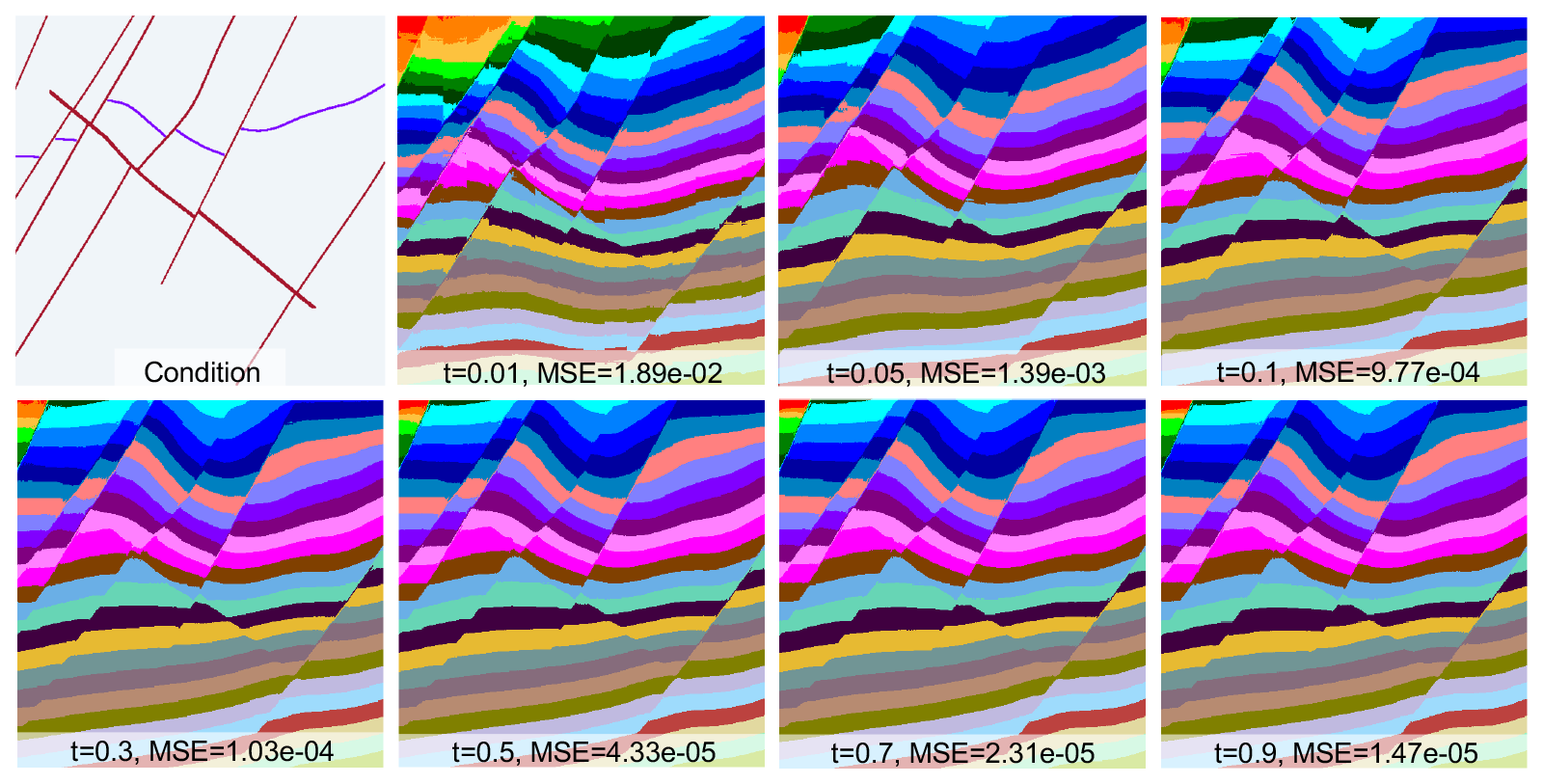
Figure 7 Single-step clean-data prediction at different noise levels. The first panel shows the input conditioning; the remaining panels show the predicted $\widehat{x}$ at t=0.01, 0.05, 0.1, 0.3, 0.5, 0.7, 0.9, using the same ground-truth sample and the same noise realization across all panels. Prediction error (MSE, relative to the ground-truth field) decreases monotonically as t increases, indicating that predictions become progressively more reliable as the noise level decreases.

Conditioning flexibility and applicability. We only consider faults and horizons as conditioning inputs in this work. For practical implicit structural modeling, additional information such as interpreted normals or orientation constraints are often beneficial, and we believe they can be incorporated naturally in our framework, either as extra input channels or as explicit loss terms. Compared with VAE-based latent diffusion, injecting such geological priors in our data-space approach is more direct and interpretable, avoiding the ambiguity of enforcing constraints in a learned latent space. Moreover, our formulation enables flexible generation of implicit structural model samples. With only a few sketched horizons and faults, the model can produce geologically realistic implicit fields, which facilitates the construction and iterative refinement of structural modeling datasets compared with traditional workflows that often rely on computationally intensive physics-based forward modeling.

Generalization capacity. The real-survey experiments (Fig. 3) provide some indication of the model's generalization capacity. Since the synthetic training data are generated using parameterized fold, fault, and unconformity rules, the model is expected to perform reasonably well when the target geological structures fall within the range of styles represented in the training distribution. However, as demonstrated in Fig. 3e, performance degrades noticeably in the presence of pronounced thrust structures, which are absent from the training dataset. This suggests that the current model should be applied with caution in tectonic settings that deviate significantly from the training distribution, such as thrust-and-fold belts. Expanding the synthetic dataset to include such structural styles would be a natural direction for future work.

Variability under sparse horizon conditioning. The horizon-sparsity ablation study (Sec.3.5) shows that the variability of the generated realizations increases as the number of horizon constraints decreases, with mean variance rising from 0.0013 (6 horizons) to 0.0073 (1 horizon). This trend is also evident from the variance maps in Fig. 4, where high-variance regions progressively expand as conditioning horizons are removed. Such behavior is expected, since regions that are weakly constrained by horizon information inherently admit a broader range of geologically plausible solutions. As the amount of conditioning information decreases, the model is afforded greater freedom in generating the implicit structural field, resulting in increased realization variability. These observations suggest that the model responds to sparse conditioning in a physically reasonable manner, producing more diverse structural realizations where geological constraints are limited.

Fault sparsity. The current framework relies on fault masks to indicate locations where structural discontinuities are permitted, and discontinuities in the generated implicit field therefore tend to coincide with the supplied fault constraints. If a fault is omitted from the conditioning data, the corresponding region is no longer explicitly identified as a discontinuity, and the model tends to preserve the smoothness of the implicit structural field there, potentially leading to weakened or absent discontinuities. A similar trend is observed in the horizon-sparsity ablation study (Fig. 4), where reducing conditioning information results in increased realization variability and structural ambiguity. Since fault masks are introduced through the same conditional mechanism, sparse or incomplete fault constraints would likewise reduce the structural information available to the model, increasing ambiguity near fault zones while favoring smoother structures in unconstrained regions. This behavior is consistent with the conditional nature of the framework, which is designed to honor the available structural constraints. In many implicit structural modeling workflows, it is desirable for the model to infer previously unidentified discontinuities even when fault information is sparse. However, this capability is not explicitly investigated in the present study. Extending the framework to identify and incorporate such missing discontinuities represents an interesting direction for future work.

Unconformities. Unconformity-related geometries are present in the synthetic training models; however, unconformities are not explicitly represented as conditioning constraints in the current framework. In this study, our primary objective was to evaluate the effectiveness of the proposed diffusion-based workflow under a simplified conditioning scheme using only horizons and faults. Consequently, the ability of the model to reconstruct unconformity surfaces has not been systematically evaluated, which we acknowledge as a limitation of the current work. Similar to faults, unconformities correspond to discontinuities in the implicit scalar field, although their geological meaning differs: faults represent stratigraphic displacement, whereas unconformities represent contact relationships between distinct stratigraphic packages. This suggests that unconformities could be incorporated as an additional conditioning channel, analogous to fault masks, together with an unconformity-aware regularization to explicitly model discontinuous stratigraphic contacts. Extending the framework in this direction represents an important avenue for future work.

Geologically impossible results. The fault-aware bending-energy loss encourages the generated implicit field to remain smooth within fault-bounded regions, which in practice is intended to suppress localized artifacts such as closed iso-surfaces (e.g., “bubbles”) that would be geologically implausible. In our experiments, we did not observe such artifacts in the generated results, suggesting that the bending-energy regularization is effective in practice. Nevertheless, under very sparse conditioning (e.g., 1 input horizon), the high-variance regions visible in Fig. 4 indicate that the model has considerable freedom in unconstrained areas, and the occurrence of geologically unreasonable structures cannot be entirely ruled out in more challenging scenarios. Incorporating additional geological rules, such as stratigraphic monotonicity constraints, into the loss function could further reduce the likelihood of such artifacts and would be a worthwhile direction for future work.

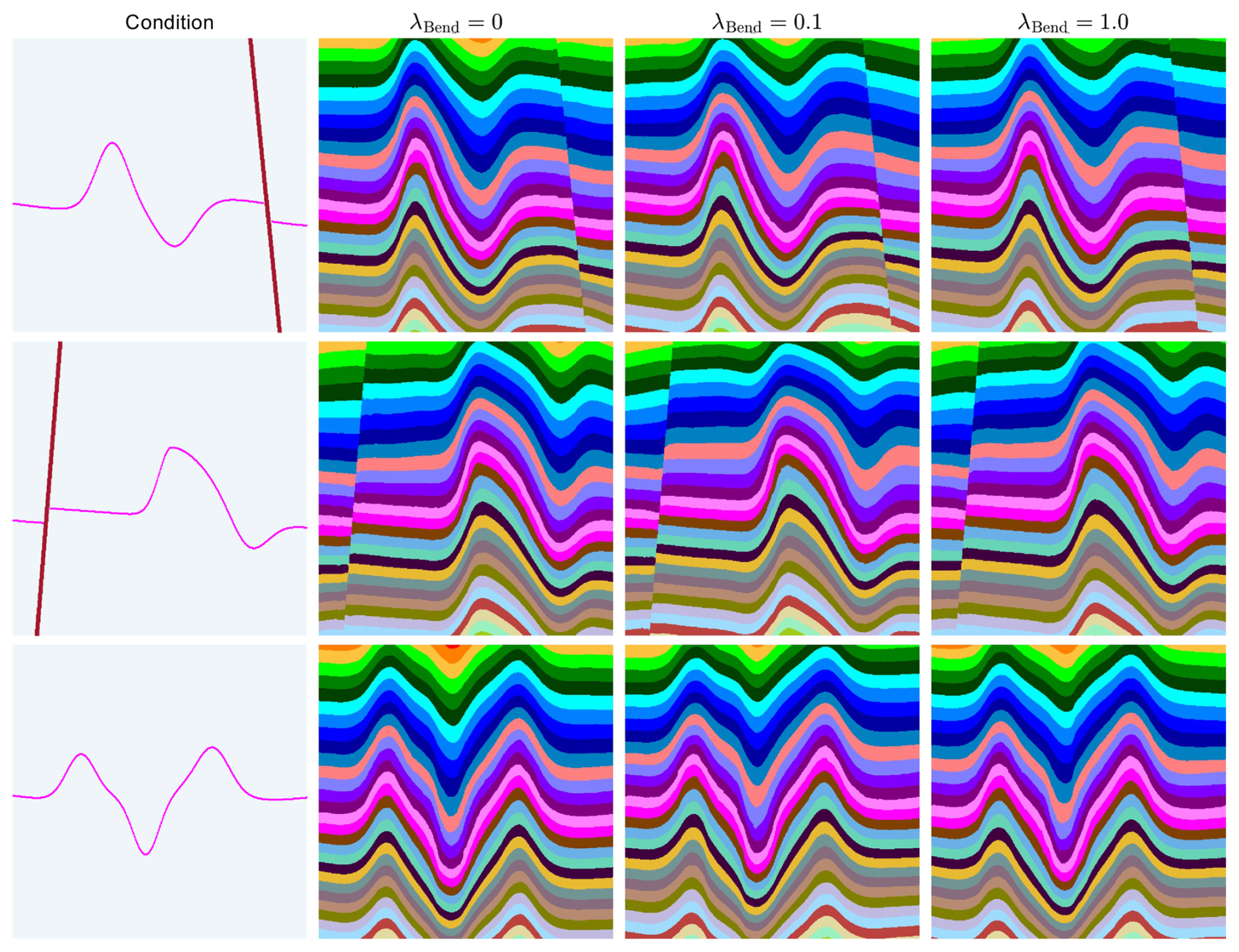
Figure 8 Sensitivity of high-curvature fold hinges to the bending-energy weight. Left column: input conditioning for three test cases, each featuring a fold hinge positioned sufficiently far from any fault: a tight anticline (top), an asymmetric fold (middle), and a double-hinge fold without any fault present (bottom). Right three columns: ensemble-mean structural models, averaged over 20 realizations from different noise seeds, generated under λ_Bend=0, 0.1, 1.0, respectively.

Preservation of high-curvature features. While the bending-energy loss suppresses geologically implausible artifacts, a quadratic penalty on curvature could, in principle, also over-smooth genuine, non-fault high-curvature features such as fold hinges. To examine this risk, we constructed several high-curvature test cases in which the fold hinges are located away from any fault (including a tight anticline, an asymmetric fold, and a double-hinge fold without any fault present). For each case, we generate 20 realizations from different noise seeds under three bending-energy weights (${\mathit{\lambda }}_{\mathrm{Bend}}\in \mathit{\{}\mathrm{0},\mathrm{0.1},\mathrm{1}\mathit{\}}$) and compare the resulting ensemble-mean structural models (Fig. 8). Even under the strongest setting (λ_Bend=1), the model accurately preserves the high-curvature geometry at these fold hinges, with no noticeable over-smoothing or structural collapse observed. Together with the quantitative results in Table 4, where reconstruction accuracy improves and realization variance does not decrease monotonically with λ_Bend, this indicates that, within the tested weight range, the regularizer does not compromise high-curvature geological features while still preserving meaningful realization diversity.

Limitation and 3D extension. This study primarily focuses on validating the effectiveness of x-prediction, the structure-enhanced transformer design, and the proposed prior-guided losses. Accordingly, our experiments are conducted on 2D implicit structural modeling, which does not fully capture 3D geological complexity such as fault connectivity and branching. Nevertheless, the proposed framework is conceptually extendable to 3D by replacing 2D patch embeddings and attention with their 3D counterparts. However, a practical 3D implementation requires additional considerations due to the substantially increased computational cost and the higher structural complexity of volumetric faulted settings. Future work will evaluate the full 3D extension, including computational scaling and constraint satisfaction in volumetric settings. Similarly, the present study assumes a uniformly sampled grid, consistent with the fixed-size patch embedding used by the ViT backbone; extending the framework to non-uniform grids, where spacing varies spatially (e.g., locally warped or flattened grids), would require rethinking the patch embedding scheme, and represents another promising direction for future work.

5 Conclusions

To eliminate reliance on VAE-based latent compression in high-dimensional diffusion modeling and overcome the difficulty of imposing geological priors in latent space, we propose LFD, a latent-compression-free, prior-guided diffusion framework with denoised-sample prediction for implicit structural modeling. LFD uses flow matching but predicts the implicit structural model directly in data space. This keeps the modeling target explicit and makes it easier to enforce geological constraints. We design a structure-enhanced ViT to improve conditioning. The network injects horizon and fault information at multiple layers. We also add two prior-guided losses. The horizon loss enforces consistency on horizon locations. The fault-aware bending-energy loss penalizes curvature only within fault-bounded regions. It avoids stencils across faults and preserves sharp discontinuities. Experiments on synthetic data and five real-survey examples with complex flower-structure faulting show that LFD produces more coherent implicit structural models than SiT. Overall, LFD demonstrates that diffusion models can effectively generate implicit structural models while directly honoring geological constraints in data space.