Hydrological auditing of LISFLOOD v4.1.1: impacts of model setup on water balance components in the Po River Basin

In recent years, large-scale hydrological models have been increasingly used at regional and global scales to support decision making. Their realism in simulating water balance components is crucial for building trust across different use cases. Hydrological models may reproduce streamflow well but misrepresent other fluxes, due to internal fluxes compensations and equifinality. Alternative setups, such as the choice of input data, model structure, and calibration methods, can influence how water is partitioned across model states and fluxes. Modellers can adjust these choices to improve the representation of the water-balance components most relevant for a given application, even when this comes at some cost to overall streamflow performance. “Hydrological auditing” of models, i.e. a thorough critical review of their realism beyond the calibration targets (usually streamflow), provides useful insights for both practical applications and process understanding. We present one such exercise in a representative European case study using a physically based hydrological model (LISFLOOD), as calibrated and set up for the European Flood Awareness System (EFAS). Originally developed for flood forecasting, LISFLOOD is increasingly also employed for drought monitoring and water resources management. We evaluate LISFLOOD v4.1.1's performance in simulating streamflow, evapotranspiration, and overall water balance in the Po River Basin, a complex and highly managed basin in Northern Italy. Six alternative model setups are tested, including different soil layers depths and preferential flow representations. Results show that the model setup currently used in EFAS v.5.0 performs best in terms of streamflow simulation, particularly at the daily time step, but tends to underestimate evapotranspiration. In turn, this may lead to an overestimation of groundwater recharge and a poor water balance representation. The use of the Budyko framework as a diagnostic tool reveals that model setups without preferential flow better match the expected long-term water balance, but reduce daily streamflow performance. The study highlights the importance of evaluating model performance and auditing alternative parametrizations to ensure accurate simulations of water balance components, crucial for water resources management. We propose diagnostic criteria to support the evaluation of physically based distributed models, across different applications, while preserving consistency in the representation of long-term water-balance components. Finally, we argue that such hydrological auditing becomes increasingly relevant as the added value of physically based models, compared to increasingly competitive data-driven models, lies in their ability to provide diagnostically useful and physically-consistent representations of internal water-balance processes.

1 Introduction

The importance of a sound quantification of hydrological variables for water resources management cannot be understated. With surging demand for adaptation to climate change and a water-resilient economy, hydrological models are increasingly called upon to support the analysis of scenarios and to inform decision making from local to regional scales (Kumar et al., 2025). They are essential tools to identify cost-effective, no-regret and, when possible, multifunctional measures enabling a rational and fair use of scarce resources, while supporting resilience and sustainable development goals (e.g., Granata and Di Nunno, 2025; Quaranta et al., 2021). Various sectoral applications, however, require an accurate representation of different hydrological variables. For example, soil moisture is key for agricultural drought monitoring and irrigation management (e.g., Zhang et al., 2025), evapotranspiration is central to vegetation and ecosystem monitoring (e.g., Fluhrer et al., 2025), groundwater storage underpins water supply planning (e.g., Abbas et al., 2025), and streamflow is essential for flood forecasting and early warning (e.g., Nearing et al., 2024), as well as hydrological drought monitoring and management (e.g., Cammalleri et al., 2017). Given the diverse application and challenges in the management of water resources, different sectors require precise estimation of specific key target variables, whose quantification should be tailored to their needs. Therefore, hydrological models should be either designed to quantify ad-hoc variables with an accuracy that aligns with the user requirements, or, in the case of process-based (semi-)distributed models, calibrated on variables other than those directly relevant for decision making, to ensure that these variables are represented in a physically consistent manner and with sufficient accuracy for the intended use case and spatial context. One prominent example of a hydrological model in use for different operational applications in the European Union, especially in large trans-boundary basins, is the open-source OS-LISFLOOD (Van Der Knijff et al., 2010). LISFLOOD is a physically based, spatially-distributed model developed by the European Commission's Joint Research Centre (JRC) and originally used for flood forecasting at European (Matthews et al., 2025b) and global scale (Matthews et al., 2025a), but later employed also in drought monitoring (Cammalleri et al., 2015, 2017) and climate change impact analysis focusing on the appraisal of water resources management measures (Bisselink et al., 2020; De Roo et al., 2021, 2023). The model is presently calibrated on the basis of streamflow observations only, as is common practice for many complex and computationally intensive large-scale hydrological models. As the needs for applications beyond the original model scope (flood forecasting) grow, it is essential to understand the extent to which the predictions for all the variables represented by the model can be trusted.

Some hydrological modelling studies have attempted to incorporate additional variables into model validation, such as evapotranspiration and soil moisture (Orth and Seneviratne, 2015), groundwater levels (Pelletier and Andréassian, 2022) and terrestrial water storage (Jensen et al., 2025). However, challenges remain even in ensuring consistency of fluxes across spatial and temporal scales, while respecting simple mass-conservation equations (Kumar et al., 2013; Samaniego et al., 2017; Ficchì et al., 2019), and observed spatio-temporal dynamics (Rajib et al., 2018; Kraft et al., 2022).

Multi-variable calibration can improve model realism but is rarely performed so far, mostly in local or regional studies (Döll et al., 2024; Guo et al., 2024) also due to data challenges, and may introduce trade-offs (Döll et al., 2024; Pelletier and Andréassian, 2022) or parameter identifiability issues (Döll et al., 2024), especially when different data sources present different error structures. Linked to this, also the sensitivity of hydrological model performances and parameters to imperfect knowledge of water fluxes and inputs, like potential evapotranspiration (Andréassian et al., 2004) and groundwater fluxes (Gleeson et al., 2021) has been rarely studied. Despite some progress over the last few decades and increased data availability especially from satellite (Huang et al., 2025), there is still limited understanding of how model parameterizations affect the internal fluxes and processes representation in large-scale models, and systematic evaluations across multiple water fluxes and storages are needed.

Such evaluations would be essential in moving towards a diagnostic approach for model evaluation that relies on hydrological theory and process understanding to support the detection of the causes of performance limitations and the resolution of model inadequacies (Yilmaz et al., 2008). This approach remains less systematic and mature than calibration practices, partly due to a lack of diagnostic evaluation criteria and structured procedures that can trace errors to specific processes or subsystems within a model. Such limitations hinder model improvements aligned with new application needs, especially when predictions beyond streamflow are required. A systematic understanding of how internal processes and water balance components behave under different model configurations of the same model and among different models is still lacking, including in LISFLOOD. This understanding becomes essential when the model is used beyond flood forecasting and addressing such a diagnostic gap is the central motivation of the present work. While we apply the approach to LISFLOOD, the diagnostic workflow we propose, based on multi-scale streamflow metrics, FDC signatures, and a cell-based Budyko-distance diagnostic, is intended as a first step towards a methodology applicable to distributed hydrological models more broadly. This contribution examines the performance of the current LISFLOOD v4.1.1 model operational setup, as incorporated in EFAS v.5.0 (see https://confluence.ecmwf.int/display/CEMS/EFAS+v5.0, last access: 10 May 2026), in terms of the overall water balance behaviour, besides the model's capability to reproduce observed streamflow. Using the Po River Basin as a test bed, we explore how the model predictions change when excluding preferential flow, a model component of LISFLOOD, and when changing the representation of soils. By comparing the EFAS v.5.0 model parametrization with a set of alternative parametrizations, we explore how these affect the model's ability to quantify hydrological variables relevant to decision making, namely evapotranspiration, runoff and infiltration. Based on our analysis, we suggest guiding criteria for the diagnostic and calibration of the model in order to improve simulations beyond the scope of flood or drought forecasting.

2 Materials and methods

2.1 The LISFLOOD model

LISFLOOD is an open-source hydrological and flood simulation model developed by the European Commission's Joint Research Centre (JRC) (Burek et al., 2013; Van Der Knijff et al., 2010). As a distributed, process-based hydrological model, it can be used to simulate the entire hydrological cycle, including rainfall-runoff processes, river routing, floodplain inundation processes, and human influence on the water system, such as water withdrawals and reservoirs. The model is currently used in two of the operational components of the Copernicus Emergency Management Service (CEMS), as it is run within the European and Global Flood Awareness Systems, i.e., EFAS (https://european-flood.emergency.copernicus.eu/, last access: 10 May 2026) and GloFAS (https://global-flood.emergency.copernicus.eu/, last access: 10 May 2026) for flood forecasting, and provides variables for drought monitoring in the European and Global Drought Observatories (EDO and GDO) (https://drought.emergency.copernicus.eu, last access: 10 May 2026). In addition, it has been used for various studies informing water-related policies, for example in evaluating nature-based solutions for water retention, as well as water savings and nutrient reduction measures on water availability and quality at the European level (Burek et al., 2012; De Roo et al., 2012). The EFAS v.5.0.0 setup covers the European continent at a spatial resolution of about 1^′ (∼1.5 km) and a temporal resolution of 6 hours. Input data can be found in the JRC data catalogue (https://data.jrc.ec.europa.eu/, last access: 10 May 2026), and model results are distributed through the CEMS Early Warning Data Store (https://ewds.climate.copernicus.eu/, last access: 10 May 2026). The model incorporates several modules representing all key hydrological processes, including a snowpack balance routine (based on the degree-day method), modules for interception of rainfall, evapotranspiration and water uptake by vegetation, a soil water balance component describing three soil layers (from the root zone to the water table), a saturation excess mechanism for rainfall-runoff transformation and a preferential flow mechanism for aquifer recharge (ByPassing the soil layers). The latter, combined with percolation from the soil, feeds an upper groundwater compartment represented as a linear reservoir, in turn feeding a lower groundwater compartment, and both contribute to streamflow with lateral flow. The model includes groundwater losses to correct for excess recharge of the lower groundwater compartment that should be in effect balanced by abstractions or transfers within aquifers. The saturation excess module is based on the conceptual Xinanjiang-VIC-Arno model (Todini, 1996), while preferential flow is described with a non-linear reservoir equation as a function of soil water content. The saturation excess and the contribution of groundwater are routed through the stream network using a kinematic wave approximation of the St.Venant equations. Lakes and reservoirs are also modelled in LISFLOOD, where regulation rules can be accounted for to simulate their impact on streamflow and water balance. In the EFAS setup, the model is currently calibrated so that the outputs match observed streamflow at a number of gauging stations across Europe by optimising an objective function, which measures the goodness of fit between model simulations and observations. The chosen goodness-of-fit criterion to optimise is the modified Kling-Gupta Efficiency (KGE) (Kling et al., 2012), commonly adopted for the calibration of hydrological models (e.g., Melsen et al., 2025). The 14 model parameters that undergo calibration are summarized in Table A1.

2.2 The Po River Basin test bed

We focus our analysis on a part of the European region covered by the EFAS setup, namely the Po River Basin in Northern Italy (Fig. A1), encompassing a total area of approximately 74 000 km². This basin combines a relatively limited extent (compared to the European domain) with a high variability of hydrological conditions, with elevations ranging from 4000 m in the Alps to the sea level at the delta, and a landscape shaped by the interplay of geological processes, such as tectonic activities, erosion and deposition (Livani et al., 2023). This landscape hosts diverse habitats, including wetlands, floodplains, and riparian forests, and plays a significant role in the biodiversity of the region, supporting various species of fishes, birds, and other wildlife. Most of the region has a mild-continental climate, with annual precipitation ranging between 750 and 1200 mm and falling mainly in spring and autumn, and average temperature from 5 to 15 °C (Vezzoli et al., 2015). The area is interesting not only for the complexity of the landscape, but also for human interactions with the water cycle: the basin generates 40 % of the Italian GDP (Musolino et al., 2018), while representing 23 % of Italian territory. Agriculture is the dominant sector in terms of water uptake (16 billion m³, 80 % of total demand) followed by municipal use (12 %) and industry (7 %). Historically water-rich, in the past decades the region has witnessed an increase in water demand contrasting with lower water availability, due to more severe droughts and long term fluctuations in streamflow (Montanari, 2012). The context underscores the importance of a correct representation of all phases of the water cycle and water storage components for decision support across sectors. Our simulations are performed with the EFAS v.5.0 setup of the LISFLOOD model, over the period 1990–2021. Within the river basin, we considered 60 streamflow gauging stations for both calibration and evaluation of the model (Fig. A1). Each station has recorded data covering between 5.5 and 23 years of daily discharge data.

2.3 Model representation of water balance components – soil, groundwater and actual evapotranspiration

This contribution focuses on the water balance components in the soil and aquifer compartments and on the representation of actual evapotranspiration (AET) in LISFLOOD. These water fluxes are empirically known to have a strong influence on other hydrological variables and processes, and model inadequacies in one of them potentially lead to spurious internal compensations with other fluxes (Ficchì et al., 2019; Le Moine et al., 2007) to close the water balance (Beven, 2001). The soil, groundwater and evaporation fluxes are difficult to measure, but bear a practical importance when it comes to water resources management (e.g., for municipal and agricultural uses). Hence, it is important to accurately represent these hydrological processes and select the respective parameters appropriately. In LISFLOOD, water that reaches the soil has two ways of moving through the soil matrix and its three layers (Fig. 1). It can either infiltrate into the unsaturated soil zone, where evapotranspiration takes place, or drain directly to the groundwater, ByPassing the unsaturated zone. The first process, based on the conceptual Xinanjiang-VIC-Arno model (Eq. 6) (Todini, 1996), is regulated by the empirical, calibrated parameter (bInfilt), which is used to approximate the saturated fraction of a model cell. The saturated fraction is then used to calculate the amount of water that becomes direct runoff (Eq. 5), representing the portion of precipitation that does not infiltrate into the soil and instead flows directly into the stream network. The preferential ByPass flow (ByPass) mechanism computes the amount of water that drains directly to the groundwater zone, given the empirical parameter (PowerPrefFlow) and the relative saturation of the soil at a given timestep (Eq. 2). The parameter PowerPrefFlow controls the rate of preferential flow, being the exponent of a power law of the relative saturation of the first two soil layers. Equations are presented here, in the same order as they are compiled in the model (see https://ec-jrc.github.io/lisflood-model/, last access: 10 May 2026, for further details).

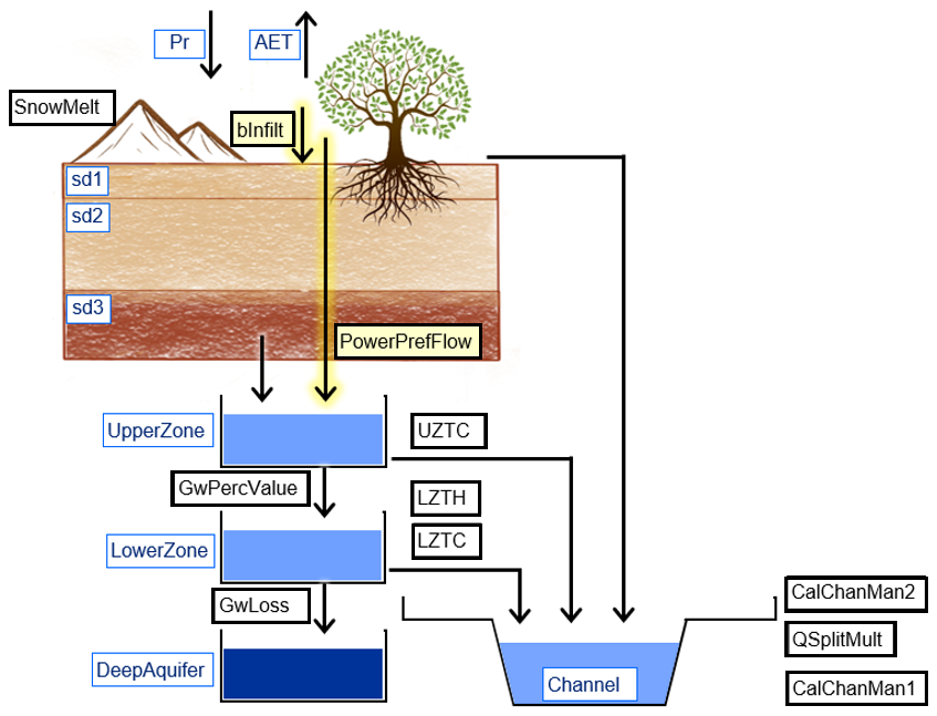
Figure 1 Schematic of the main processes of LISFLOOD model. Water fluxes are represented by arrows, with the infiltration and preferential flow processes (and respective parameters) highlighted in yellow. For visual clarity, only 11 of the 14 calibrated parameters are shown in bold black; the remaining 3 parameters, which relate to lake and reservoir dynamics, are not included in the figure but are listed in Table A1, while the main processes and model compartments are reported in blue.

First, the preferential flow is calculated from the relative saturation (RelSat) of the first two soil layers, and the potential Available Water for Infiltration (AWI), which represent the net precipitation and leaf drainage that reaches the soil surface, as:

$$\begin{array}{}\text{(1)}& {\displaystyle }& {\displaystyle }{\mathrm{AWI}}_{\mathrm{pot}}=\mathrm{precipitation}+\mathrm{LeafDrainage}-\mathrm{Interception}\text{(2)}& {\displaystyle }& {\displaystyle }\mathrm{PrefFlow}=\left({\mathrm{RelSat}}^{\mathrm{PowerPrefFlow}}\right)\cdot {\mathrm{AWI}}_{\mathrm{pot}}\text{(3)}& {\displaystyle }& {\displaystyle }\mathrm{AWI}={\mathrm{AWI}}_{\mathrm{pot}}-\mathrm{PrefFlow}\end{array}$$

where PowerPrefFlow is a calibrated model parameter. The remaining water (Eq. 3) is then partitioned between direct runoff (Eq. 5) and water seeping into the unsaturated zone as Infiltration (Eq. 4).

$$\begin{array}{}\text{(4)}& {\displaystyle }& {\displaystyle }\mathrm{Infiltration}=\max \left(\min \right(\mathrm{AWI},\mathrm{InfiltrationPot}),\mathrm{0}.)\text{(5)}& {\displaystyle }& {\displaystyle }\mathrm{Runoff}=\mathrm{AWI}-\mathrm{Infiltration}\end{array}$$

where Infiltration Potential (InfiltrationPot) is calculated using the Xinanjiang-Arno model formulation (Todini, 1996) as:

$$\begin{array}{}\text{(6)}& \begin{array}{rl}\mathrm{InfiltrationPot}& =\mathrm{StoreMaxPervious}\\ & \cdot (\mathrm{1.0}-\mathrm{SatFraction}{)}^{\mathrm{PowerInfPot}}\end{array}\end{array}$$

and StoreMaxPervious and PowerInfPot are equal to:

$$\begin{array}{}\text{(7)}& {\displaystyle }& {\displaystyle }\mathrm{StoreMaxPervious}=\mathrm{WS}\mathrm{1}/(\mathrm{bInfilt}+\mathrm{1})\text{(8)}& {\displaystyle }& {\displaystyle }\mathrm{PowerInfPot}=(\mathrm{bInfilt}+\mathrm{1})/\mathrm{bInfilt}.\end{array}$$

where WS1 is the maximum soil moisture for soil layers 1 and 2 in mm, PowerPrefFlow and bInfilt (highlighted in yellow in Fig. 1) are two of the 14 model calibrated parameters (Table A1), and specifically, they are among the 7 calibrated parameters that characterize the unsaturated and saturated soil zones. While a calibration of the model can elicit combinations of the parameters that reproduce observed streamflow to a comparable extent, different combinations of bInfilt and PowerPrefFlow may lead to very different simulations of the soil wetness, aquifer state and AET. As both saturation excess and ByPass flow are modelled empirically and independently, the calibration of the two parameters based only on the streamflow target does not guarantee to yield a physically consistent representation of soil water flows. This in turn influences also other model water-balance components. For example, the water content in the first 2 soil layers of the unsaturated zone (i.e., RelSat) represents the water available to plants for transpiration, which depends on soil saturation. Moreover, when the soil water content is low and cultivations lack sufficient water, the irrigation module is triggered and activates water withdrawal from surface and groundwater. As a consequence, the inaccurate representation of soil wetting and drying can translate into a over/underestimation of both actual evapotranspiration and water usage in agriculture.

Another aspect of crucial importance is the assumed soil depth. This largely determines the maximum amount of water available for soil and plants transpiration, however its elicitation remains challenging (e.g., Fan et al., 2019). Unlike in other distributed models, such as VIC, (Hamman et al., 2018), in LISFLOOD soil depth is not a calibrated parameter. LISFLOOD considers 3 soil layers: the first is the superficial soil (sd1) with a fixed depth (50 mm), while the depths of the second (sd2) and third (sd3) layers are assigned on the basis of soil properties derived from external data sources (e.g., depth to bedrock, depth to water table), as described in Sect. 2.4. LISFLOOD accounts for water redistribution across the soil layers, but evapotranspiration (constrained not only by energy but also by available water) occurs only in the first 2 soil layers, which represent the superficial and upper soil extending to the roots depth. Obviously, the chosen representation of soil layers depths has a potentially strong impact on model calibration, model performance and overall water balance. Finally, the model has two parameters controlling the recharge of the lower from the upper aquifer (GwPercValue), and the leakage of water from the lower to the deep aquifer (GwLoss). These add flexibility in the production of streamflow, but their values reverberate in the aquifer water balance. The purpose of this study is to explore how different parametrizations of the LISFLOOD model influence its performance in reproducing streamflow, soil water balance and AET. In particular we test the effect of (i) excluding the ByPass flow mechanism (highlighted in yellow in Fig. 1) and (ii) using different soil depth configurations, since they both play a role in how water moves through the soil, hence affecting the soil water balance and the representation of AET.

2.4 Setup of numerical experiments

We design five new different model experimental setups (Table 1) and we compare the results against the current EFAS setup, considered as the benchmark. Two new configurations for soil depth 2 and soil depth 3 were designed by adopting different parametrizations. The same alternative model configurations, including the one with the original soil depths, were also calibrated excluding the ByPass mechanism, meaning that water can reach the groundwater compartment only through the unsaturated soil zone. Besides that, the input data used for all setups was identical to the one used for the benchmark model, which consist in 60 streamflow stations (used for model calibration), same static parameters (Choulga et al., 2024) and gridded time series of weather forcings from the EMO-1, European Meteorological Observations (v1) dataset (Thiemig et al., 2022), based on observational data from over 35 000 weather stations over Europe, and covering the period 1990–2021 at 6-hourly timestep for precipitation and temperature (Thiemig et al., 2022). The new soil configurations were calibrated following the same calibration routine of EFAS v.5.0 (ECMWF, 2022).

(Hengl et al., 2017)(Fan et al., 2013)

Table 1 Description of tested model setups, with 3 different soil depth configurations (including the benchmark, i.e., EFAS v.5.0) and with/without the preferential (ByPass) flow mechanism.

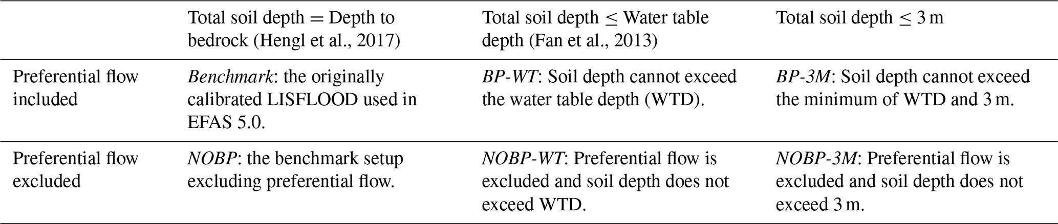
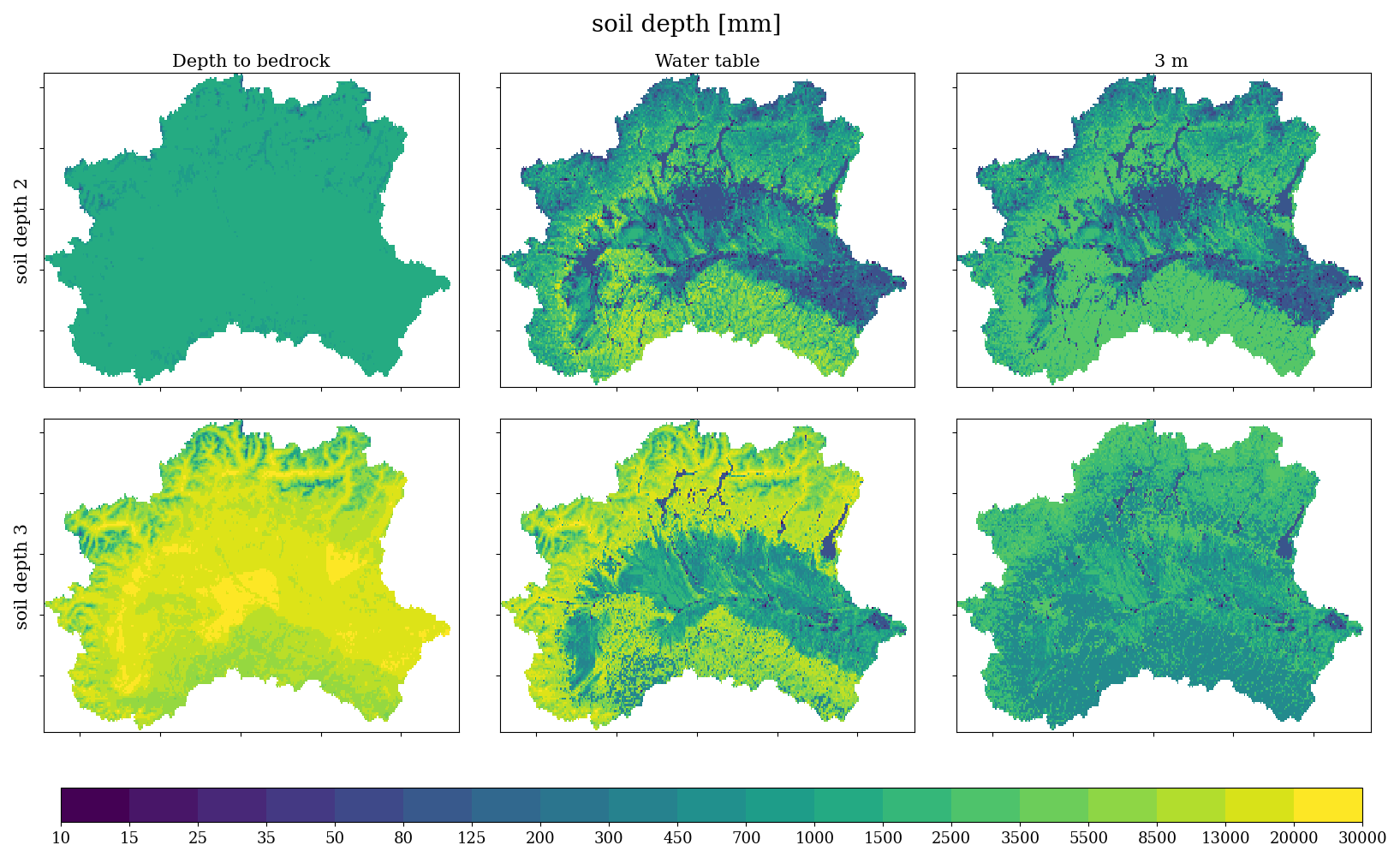
Figure 2 Soil depth (in millimeters) of soil layers 2 and 3 for the three alternative soil configurations used in our experiments.

The three soil depth configurations (the benchmark and the two new representations) for layers 2 (sd2) and 3 (sd3) are shown in Fig. 2. The benchmark soil depth configuration is the current setup (EFAS v.5.0), derived from the so-called “Absolute depth to bedrock” dataset from ISRIC (Hengl et al., 2017) and the root depth of forest and non-forest vegetation from FAO (Choulga et al., 2024). The second soil depth configuration assumes depth as the minimum between the ISRIC depth to bedrock data and the water table depth (WTD) derived from the dataset of Fan et al. (2013); in this second configuration, roots depth was also taken from another study (Fan et al., 2017), and used to compute the thickness of the soil depth of the second layer following the methodology from Burek et al. (2013). The third layer depth configuration is estimated as for the second, except in that it limits the maximum soil depth to 3 m, consistent with the upper range of soil depths historically used in operational LISFLOOD setups (Laguardia and Niemeyer, 2008) and representing a moderate extension of the 2 m baseline typical of global soil datasets, which has been shown to be too shallow to capture deeper groundwater dynamics (Mendoza et al., 2025).

The five new model configurations were calibrated, following the same methodology used to calibrate EFAS v.5.0 (ECMWF, 2022). The calibration tool, based on the DEAP algorithm (Fortin et al., 2012), was employed and the sub-catchments draining to the 60 river gauge stations were calibrated following a nested approach, where head-catchments are calibrated first and then the simulated streamflow at their outlets (as calibrated) is the input of the downstream sub-catchment. A total of 14 parameters are calibrated in the two experiments with the active ByPass feature (BP-WT and BP-3M), as listed in Table A1, the benchmark is run with the EFAS v.5.0 calibrated parameters. In contrast, in the three experiments without the ByPass mechanism, 13 parameters are calibrated, excluding the PowerPrefFlow parameter, which specifically controls the preferential flow mechanism. Across the entire EFAS domain (Europe), the model operates at a 6-hourly timestep. This enables sub-daily calibration where sub-daily observations are available. For stations where only daily observations are available, the model output is temporarily resampled to match the daily timestep observations. For the Po Basin study area, only daily time series data were available at all 60 stations. The calibration process uses the modified Kling-Gupta Efficiency (KGE) (Kling et al., 2012) as the objective function, which is described in the following section.

2.5 Model performance criteria

2.5.1 Comparison with observed streamflow

We compare the six model setups presented above against observed streamflow at daily, monthly, and yearly time step. The comparison is mainly based on the modified Kling–Gupta Efficiency (KGE) (Kling et al., 2012), which is also used as objective function for model calibration. In addition, we analyse its three components: correlation, bias ratio and variability (or spread) ratio, to characterise the performance on these three basic aspects. KGE is defined as one minus the Euclidean Distance (ED) of these components, computed as function of simulated and observed streamflows, from their ideal values, as follows:

$$\begin{array}{}\text{(9)}& \mathrm{KGE}=\mathrm{1}-\sqrt{(r-\mathrm{1}{)}^{\mathrm{2}}+(\mathit{\beta }-\mathrm{1}{)}^{\mathrm{2}}+(\mathit{\gamma }-\mathrm{1}{)}^{\mathrm{2}}}\end{array}$$

where β is the bias ratio (i.e., ratio of mean simulated over mean observed flow), r is the Pearson correlation coefficient and γ is the variability ratio (i.e., ratio of the coefficients of variation). The ideal value of the KGE components r, γ and β is 1, resulting in a ED of these components equal to zero, which then maximizes the value of KGE. The KGE on untransformed streamflow is based on model residuals that are higher for high flows and consequently tend to give less prominence to errors on low flows (Santos et al., 2018; Garcia et al., 2017). While appropriate for flood applications, this objective function may not ensure a balanced model calibration when looking at low flows or at average regimes, which are crucial for drought monitoring and water resources applications.

To evaluate how different model configurations affect various flow regimes, including low flows, in addition to the KGE computed over the whole time series of flows, we evaluate the simulated flow duration curve (FDC) and key behavioural catchment functions using four signature metrics (Yilmaz et al., 2008): the percent bias in overall runoff ratio (%BiasRR), the percent bias in FDC midsegment slope (%BiasFMS), the percent bias in FDC high-segment volume (%BiasFHV), and the percent bias in FDC low-segment volume (%BiasFLV).

The %BiasRR is a signature measure of overall water balance and indicates whether the model over- or under-estimates (when positive or negative, respectively) the runoff compared to observations.

$$\begin{array}{}\text{(10)}& \mathit{\%}\mathrm{BiasRR}={\displaystyle \frac{Q_{\mathrm{sim}}-Q_{\mathrm{obs}}}{Q_{\mathrm{obs}}}}\times \mathrm{100}\end{array}$$

where Q_obs is the observed streamflow and Q_sim is the simulated streamflow.

The %BiasFMS represents the percent bias of the slope of the mid-segment of the FDC, between 0.2–0.7 flow exceedance probabilities. Positive values indicate that the model overestimates the slope of the midsegment (steeper, and hence flashier than observed), while a negative %BiasFMS indicates underestimation (flatter slope than observed). Ideally, %BiasFMS should be close to zero, indicating good agreement between observed and simulated mid-segment slopes. The FDC midsegment slope can be seen as a signature of vertical redistribution of soil moisture, hence of soil storage capacity, with the importance of overland flow being larger for steeper slopes, while a slower and more sustained groundwater flow response is associated to flatter midsegment slopes.

$$\begin{array}{}\text{(11)}& \begin{array}{rl}& \mathit{\%}\mathrm{BiasFMS}=\\ & {\displaystyle \frac{\left[\log \left(Q_{\mathrm{sim},\mathrm{m}\mathrm{1}}\right)-\log \left(Q_{\mathrm{sim},\mathrm{m}\mathrm{2}}\right)\right]-\left[\log \left(Q_{\mathrm{obs},\mathrm{m}\mathrm{1}}\right)-\log \left(Q_{\mathrm{obs},\mathrm{m}\mathrm{2}}\right)\right]}{\left[\log \left(Q_{\mathrm{obs},\mathrm{m}\mathrm{1}}\right)-\log \left(Q_{\mathrm{obs},\mathrm{m}\mathrm{2}}\right)\right]}}\\ & \times \mathrm{100}\end{array}\end{array}$$

m1 and m2 refer to the 0.2 and 0.7 flow exceedance probabilities.

The percentage bias in high (%BiasFHV, 0–0.02 flow exceedance probabilities) and low (%BiasFLV, 0.7–1.0 flow exceedance probabilities) flow segment volumes are used to assess the goodness of fit of the extreme high and low portions of the FDC, respectively. Positive values indicate an overestimation of high/low flows by the model. The ideal value is zero for both, which indicates that the model is perfectly able to reproduce high/low flows. As hydrological signatures, the %BiasFLV indicates the goodness of fit in long-term baseflow response (as the total volume of the low-flow segment can be seen as an index of baseflow response), while the %BiasFHV is associated to the level of both vertical and temporal redistribution of water.

$$\begin{array}{}\text{(12)}& {\displaystyle }& {\displaystyle }\mathit{\%}\mathrm{BiasFHV}={\displaystyle \frac{\sum _{h=\mathrm{1}}^H\left(Q_{\mathrm{sim},h}-Q_{\mathrm{obs},h}\right)}{\sum _{h=\mathrm{1}}^H{Q}_{\mathrm{obs},h}}}\times \mathrm{100}\text{(13)}& {\displaystyle }& {\displaystyle }\mathit{\%}\mathrm{BiasFLV}={\displaystyle \frac{\sum _{l=\mathrm{1}}^L\left(Q_{\mathrm{sim},l}-Q_{\mathrm{obs},l}\right)}{\sum _{l=\mathrm{1}}^L{Q}_{\mathrm{obs},l}}}\times \mathrm{100}\end{array}$$

where h=1, 2, … H are the flow indices for flows within the respective exceedance probabilities intervals.

Results are considered satisfactory when bias values are within the ±30 % range and unsatisfacory when greater than ±30 % as summarized by Cislaghi et al. (2020) from previous literature (Herbst et al., 2009; Mendoza et al., 2015; Pfannerstill et al., 2014).

2.5.2 Compliance with the Budyko functional relationship

Besides comparison of model simulations against streamflow observations, it has been proposed that models should be also verified against empirical functional relationships that are commonly observed in hydrological data (Gnann et al., 2023; Yilmaz et al., 2008), among which the well-known Budyko model (Budyko, 1974) is probably the most commonly used. Sometimes referred to as the Turc-Budyko non dimensional graph (Coron et al., 2015; Turc, 1954), the Budyko model describes the long-term annual average water balance of a catchment, using a simple empirical equation that relates the long-term annual evaporative index, i.e., long-term mean annual actual evapotranspiration (AET) divided by long-term mean annual precipitation (Pr), to the aridity index, which is equal to mean annual potential evapotranspiration (PET) divided by mean annual Pr. This relationship can be interpreted, hydrologically, as arising from the competition between energy and water availability (Chen and Sivapalan, 2020). Although many alternative forms of the relationship have been proposed in the literature (Andréassian and Perrin, 2012; Chen and Sivapalan, 2020), here we refer to the original, non-parametric equation given in Budyko (1974):

$$\begin{array}{}\text{(14)}& \mathrm{\Psi }=\mathit{\varphi }{\left[\tanh \left({\mathit{\varphi }}^{-\mathrm{1}}\right)\cdot \left(\mathrm{1}-e^{-\mathit{\varphi }}\right)\right]}^{\mathrm{0.5}}\end{array}$$

where Ψ is the evaporative index AET/Pr and ϕ is the aridity index PET/Pr. A key assumption is that variations in catchment storage are insignificant in the long term and that the catchment remains a closed water system, unaffected by anthropogenic influences and not exchanging water with other catchments. Since the LISFLOOD model operates as a column model without lateral flow between cells, each grid cell can be considered a small, isolated catchment. Under these assumptions, we expect that, over long timescales, the behaviour of an individual cell will conform to the Budyko curve. Grid cells affected by substantial anthropogenic influences were excluded, by removing those with more than 80 % irrigated crops, or 80 % sealed surface, and with 100 % open water and rice cultivation (see AppendixA), since these characteristics would cause deviations from the assumptions under which the Budyko model is valid.

For each pixel in the modelled domain, the aridity index, PET/Pr, and the evaporative index, AET/Pr, have been calculated for each experiment and compared against the Budyko curve. Under such conditions, the model allows to detect the mean “climatological” AET, enabling the estimation of average annual water surplus from the catchment, and consequently of the annual streamflow volume. Indeed, any surplus of precipitation with respect to AET would practically coincide with the streamflow volume (Q), from the closure of the water balance ($Q=P-\mathrm{AET}$), in absence of human withdrawals and of natural inter-catchment groundwater flows (e.g. Ballarin et al., 2022). The framework has been extensively used to identify catchments undergoing shifts in water balance due to climate change (Senbeta et al., 2023), impact of land use change on runoff generation (Gnann et al., 2023; Jaramillo and Destouni, 2014). Given its simplicity, the Budyko framework offers a tool to evaluate (Gnann et al., 2023; Koppa et al., 2021) and/or calibrate (Greve et al., 2020) complex hydrological models. In previous tests at the European scale (Pistocchi et al., 2019) and, more specifically, in the Danube catchment (Pistocchi et al., 2015), it has been shown that the Budyko relationship predicts observed annual average streamflow volumes quite accurately; for the Danube, the comparison yields a correlation of 0.89, a relative mean error of +8 %, and a relative standard deviation error of +9 %. These findings have been confirmed by a more recent analysis, showing that the Budyko relationship generally predicts annual streamflow volumes well in line with observations in several European catchments (Pistocchi et al., 2024). The deviation of simulated AET and runoff from the predictions of the Budyko equation highlights situations where AET or runoff differ significantly from what one would expect based on the climatological characteristics of the catchment. We measure the relative difference of AET/Pr and Q/Pr from the values predicted with the above Budyko equation, that we call Budyko Distance (BD), for each grid cell of the modelled study area using the formula:

$$\begin{array}{}\text{(15)}& {\displaystyle }& {\displaystyle }{\mathrm{BD}}_{\mathrm{AET}}={\displaystyle \frac{{\mathrm{AET}}_{\mathrm{sim}}-{\mathrm{AET}}_{\mathrm{budyko}}}{{\mathrm{AET}}_{\mathrm{budyko}}}}\text{(16)}& {\displaystyle }& {\displaystyle }{\mathrm{BD}}_Q={\displaystyle \frac{Q_{\mathrm{sim}}-Q_{\mathrm{budyko}}}{Q_{\mathrm{budyko}}}}\end{array}$$

where AET_budyko\Q_budyko is the long-term AET\ calculated using the Budyko equation (Eq. 14) and AET_sim\Q_sim is the long-term AET simulated by the model. The closer BD is to zero, the more consistent is the model long-term partitioning of Pr between Q and AET with the expected Budyko relationship. In practice, we consider results “Budyko compliant” when BD is between −0.2 and 0.2 (±20 %), in line with previous studies (Li et al., 2014; Gentine et al., 2012), where a general acceptance was set to a 10 % difference from AET_budyko, but larger deviations could occur for other physical reasons, such as vegetation and land-use changes, (Gunkel and Lange, 2017; Jaramillo and Destouni, 2014) as well as snow dynamics and snow fraction changes (Zaerpour et al., 2024).

2.5.3 Water balance closure

For a hydrological model, we expect the water balance to close, meaning that in the long term the cumulative precipitation should equal the sum of cumulative actual evapotranspiration, cumulative streamflow volume, and cumulative net groundwater exchanges due to sub-surface connectivity. LISFLOOD, being a column model, does not simulate inter-catchment groundwater inflows, but ground water losses instead. In closed topographic catchments, groundwater losses are often introduced to ensure the water balance closure and compensate for excessive groundwater recharge. A large contribution of groundwater losses indicates either that the catchment leaks a groundwater volume to neighbouring catchments or that the water balance calculation is unable to explain where the corresponding volume should be allocated, thus adjusting it with large losses. For the Po Basin, however, such gains are assumed to be negligible because the dominant groundwater flow paths and aquifer boundaries lie within the surface-water catchment (Beretta et al., 2025). Based on these considerations we compare the performance of different model setups also in terms of how they break down precipitation in the various components of the water balance. This holds insofar as we neglect the changes in the internal storage of the system (snow, lakes and reservoirs, soil and aquifer water content), which is an acceptable assumption over an extended multi-year period.

3 Results

3.1 Streamflow

Across the 60 calibrated sub-catchments, model performance is primarily controlled by the representation of preferential flow, with soil depth playing a secondary role (Fig. 3). At the daily scale, setups including the ByPass mechanism consistently achieve higher KGE values, while those without ByPass perform worse, regardless of soil depth. The setups with the ByPass mechanism perform in the same way (yielding almost identical KGE values), irrespective of the assumptions on soils. For the setups without ByPass, a slight improvement is observed when soil thickness is reduced (moving from NOBP to NOBP-3M), but the difference remains small compared to the gap between ByPass and no-ByPass configurations. The main cause of the KGE performance decline for the setups without ByPass is the degradation of the correlation, followed by the variability ratio, while the bias remains nearly identical across all setups and timescales (Friedman test p value above 0.05). This suggests that the ByPass has an essential role in the temporal redistribution of water in LISFLOOD that cannot be easily compensated by other model components, while its contribution in the long-term water balance could be easily replaced. At the monthly and especially annual scales, the performances are more similar than at daily scale for all models, as shown by the increasing p value in KGE. In this case, the setup without ByPass and with the thinnest soils (NOBP-3M) achieves the same performance as all setups with ByPass (with negligible differences), while thicker soils cause a worsening of the performance in the absence of ByPass.

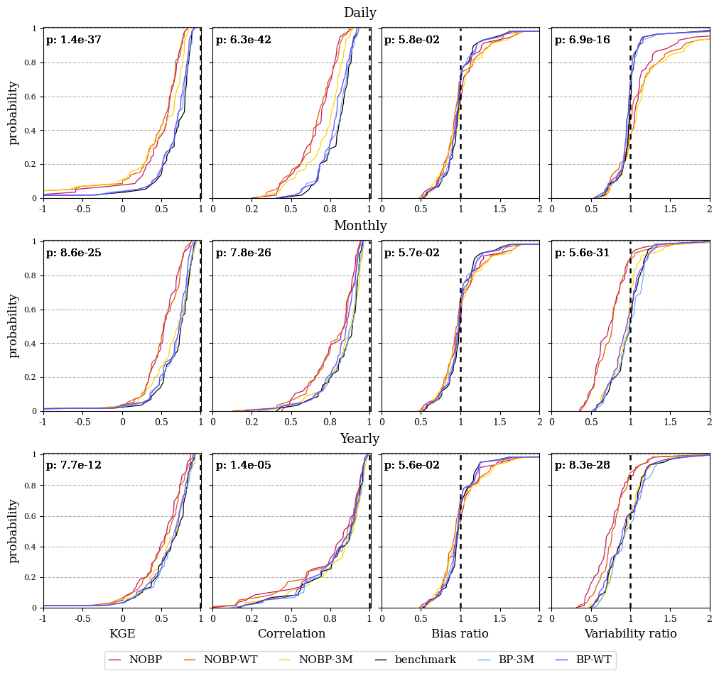
Figure 3 Empirical cumulative distribution functions (CDFs) of KGE and its three components (correlation, bias and variability ratio) across all the 60 calibrated sub-catchments for the six LISFLOOD setups (including the benchmark), evaluated at daily (top row panels), monthly (middle panels) and yearly (bottom panels) time scale. In the top left corner of each plot, the minimum p value for all pairs of the Friedman test (FT) is shown: p>0.05 indicates no significant differences among the six LISFLOOD setups, while p<0.05 indicates significant differences.

The spatial patterns of overall daily performance confirm the consistent advantage of including the ByPass mechanism, as setups with ByPass achieve higher KGE values across the basin (Fig. B1). The largest difference in performance is seen in the western part of the basin and in the floodplain, downstream (southern) catchments. In contrast, sub-catchments in the northeastern part of the basin exhibit poorer performance than the basin average, regardless of the presence or absence of the ByPass. A larger number of catchments (up to 3 additional cases) have a KGE below −0.41, meaning that the model is worse than a simple mean flow benchmark (Knoben et al., 2019), when the ByPass is excluded. An analysis of the single components of KGE (Figs. B2–B4) reveals that the correlation degrades across the whole catchment in the experiments without ByPass; the variability ratio generally worsens in all experiments, especially in catchments in the north part of the basin; the bias ratio does not show major differences across the basin.

The most frequently best-performing setups are BP-3M and the benchmark, dominating respectively in the western and southern parts of the basin (see Fig. B5). The setups with ByPass enabled perform best in almost all sub-catchments, with only four Alpine sub-catchments in the north-east showing negligible differences. Even if each of the different soil configurations with active ByPass leads to the best performance in several cases, most catchments exhibit negligible differences in performance by changing only the soil depth. On the other hand, without ByPass the three soil configurations show substantial differences, with a general better performance of NOBP-3M (thinnest sd3 soil), especially in the floodplain, whereas in the Alpine sub-catchments the differences are negligible.

3.2 Flow duration curve

Flow duration curve (FDC) diagnostics reveal clear differences between setups, with the representation of preferential flow strongly shaping model behaviour, especially across average and high-flow regimes as revealed by %BiasFMS and %BiasFHV (Fig. 4).

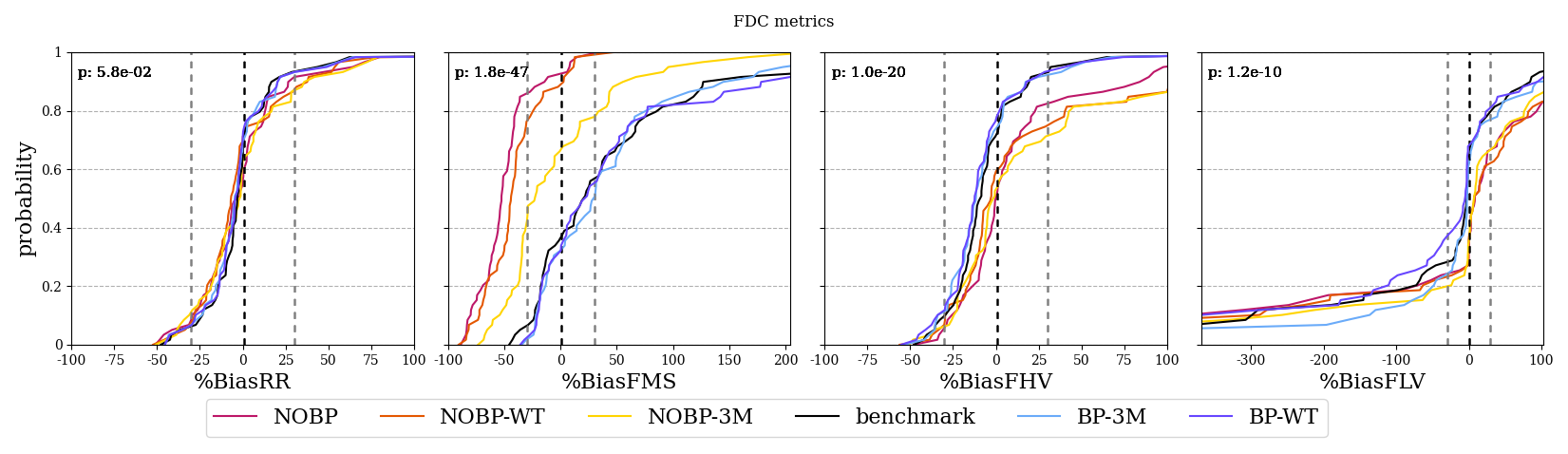
Figure 4 Flow duration curve (FDC) signature metrics (%BiasRR, %BiasFMS, %BiasFHV, %BiasFLV); the black dashed vertical line indicates the optimal values, while the grey dashed lines define the acceptability range at ±30%.

Overall water balance bias (%BiasRR) is comparable across all the experiments, with slightly better performance when the ByPass is enabled. In contrast, the mid-segment of the FDC (%BiasFMS) shows the most marked differences: in all experiments without the ByPass, more than 60 % of the catchments exhibit negative values, indicating overly sustained/slow-varying flows compared to observations, while this behaviour is much less frequent with ByPass (below 40 %); this problem is most pronounced in NOBP and NOBP-WT, where only ≈10 % of the catchments fall within the ±30 % acceptability range. The best performing experiment without the ByPass is the NOBP-3M with 40 % of catchments within the acceptability range. The experiments with ByPass show broadly similar behaviour, with more than 60 % of simulations being more flashy than observations and 50 % of catchments within the acceptability range. High-flow performance (%BiasFHV) is also generally better in the experiments with ByPass, as they show ≈85 % of the stations within the acceptability range, while these drop substantially without ByPass. Among the no-ByPass experiments, NOBP performs best, followed by the NOBP-WT and the NOBP-3M.

Low flows (%BiasFLV) are more problematic across all experiments: only ≈40 % and ≈55 % of catchments fall within the acceptability range (±30 %), in the experiments without and with ByPass respectively. In the no-ByPass experiments, the model tends to overestimate low flows more frequently than with ByPass. In terms of %BiasFLV, the BP-3M experiments is the best performing among the experiments with the ByPass active, with more than 50 % of the catchments within the acceptability range. The benchmark and the BP-WT experiments tend to have more catchments where low flows are underestimated.

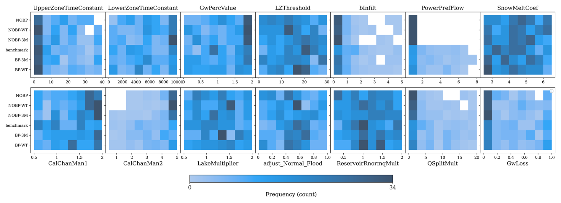
Figure 5 Frequency distributions of the 14 calibrated parameters values across the 60 sub-catchments for each of the six experiments. Colour shades represent the frequency of occurrence of a parameter within the values on the horizontal axes. Darker shades indicate more frequent parameter values. Patterns of vertical bands suggest stability across experiments, while shifts in distribution reflect sensitivity to model setup.

3.3 Calibrated parameters

The frequency distributions of the 14 calibrated parameters across the 6 experiments highlight how parameter sensitivity depends on the model setup (Fig. 5).

We tested whether the calibrated parameter distributions differ between the benchmark and each alternative setup using two complementary distributional tests: the Kolmogorov–Smirnov (KS) test and the 2-Wasserstein-distance-based (WD) test of Schefzik et al. (2021), already applied in a hydrological context by Ficchì et al. (2026). Both tests were corrected for multiple comparisons using the Benjamini–Hochberg procedure (Benjamini and Hochberg, 1995) at the 0.05 significance level. The paired shifts of each parameter for each setup against the benchmark, together with the test outcomes, are reported in Appendix B (Figs. B6 and B7). The KS test is sensitive to localised differences between empirical cumulative distribution functions, while the WD test captures bulk distributional shifts and differences in location, size, and shape. All the experiments including the ByPass do not show significant differences in the frequency distributions of the calibrated parameters compared to the benchmark (Fig. B6), with the exception of a modest downward shift in bInfilt detected by the WD test for both BP-WT and BP-3M, suggesting that changes in soil depth do not cause substantial changes in other parameters and do not lead to systematic internal flux compensations.

In contrast, the experiments without ByPass show systematic and consistent shifts in several parameters, pointing to more pronounced internal compensations in the absence of preferential flow. Both tests agree on significant shifts for bInfilt, CalChanMan1, CalChanMan2, and QSplitMult across all three no-ByPass setups (Fig. B6). The KS test additionally detects shifts in UpperZoneTimeConstant (NOBP-WT, NOBP-3M) and LowerZoneTimeConstant (NOBP-3M), which we interpret as tail-localised changes in the residence times of the upper and lower groundwater zones. These parameters affect the speed of propagation of floods, the speed of water flowing in the channel and floodplain, the saturation excess, and the speed of water reaching the channel from the fast and slow saturated soil zone. The distribution of these calibrated parameters for each catchment is shown in Appendix B (Figs. B8–B13). Compared to the ByPass setups, the changes in routing parameters (CalChanMan2 and QsplitMult) in the experiments without the ByPass suggest slower channel routing (higher value of CalChanMan2) and greater diversion to floodplains or to the overbank part of the channel (lower QsplitMult). Soil-groundwater parameters adjust by clearly compensating the lack of the ByPass component: bInfilt shows a significant decrease, indicating that water infiltrates more in the unsaturated zone; the decrease of the UpperZoneTimeConstant and the increase of the LowerZoneTimeConstant indicate respectively an increase and a decrease of residence time of the fast and slow saturated zone. GwLoss (Fig. B10), even if no significant changes are detected by KS and WD tests, tends to be lower meaning that there is less need to compensate for excess water in the deep aquifer that cannot be explained by other physical processes. Overall, excluding the ByPass forces compensatory parameter adjustments that redistribute water through alternative pathways, replacing the aquifer recharge otherwise captured by the preferential flow process.

3.4 Compliance with the Budyko functional relationship

3.4.1 Evapotranspiration

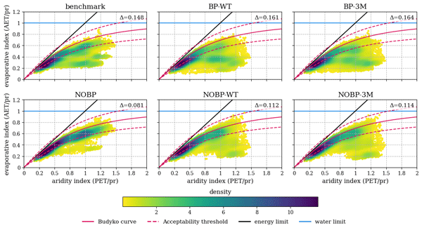
The setup with no ByPass and original soil configuration (NOBP) shows the pattern with the highest overall proximity to the Budyko curve (see Fig. 6; mean distance: 0.081), followed by other setups without ByPass (NOBP-WT and NOBP-3M). Among the experiments with the ByPass, the benchmark is the one performing best (mean distance from the Budyko curve equal to 0.148). The other setups with ByPass (BP-WT and BP-3M) approach the Budyko curve when AET/Pr < 0.5 and PET/Pr < 0.4, while at higher PET/Pr levels there are many more cases farther from the Budyko curve. The same trend is visible, but weaker, with the other setups without ByPass (NOBP-WT and NOBP-3M). This indicates that when the soil depth is the same, excluding the ByPass tends to improve the compliance with a Budyko functional relationship for evapotranspiration. The spatial distribution of the distance from the expected Budyko evapotranspiration clearly highlights a “patchy” pattern (Fig. B14), especially in the ByPass experiments, which resembles the distribution of the bInfilt (Fig. B8) and PowerPref (Fig. B9) parameters. In general, for most of the basin the modelled AET is lower compared to the AET calculated using Budyko, highlighting a widespread non-compliance, especially for setups with the ByPass. Budyko non-compliance is also particularly visible where soil depth of the second layer is thin, as for example east of the floodplain, where soil depth is below 50 cm for NO/BP-WTD (Fig. 2), and the actual evaporative index is half as expected by Budyko.

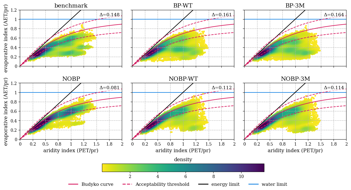
Figure 6 Density plot of Aridity Index vs Evaporation Index of each pixel of the masked Po River Basin domain; the magenta curve represents the Budyko relationship (described in Eq. 14) and the dotted magenta curve the acceptability range. On the top right corner of each plot the average distance (adimensional) of each pixel from the Budyko curve is indicated. The points falling between the dotted and continuos magenta lines are considered Budyko compliant. The blue line represents the water limit, where AET < P, and the black line represents the energy limit, where AET ≤ PET. Those two limits cannot be exceeded in systems that comply with the Budyko hypothesis.

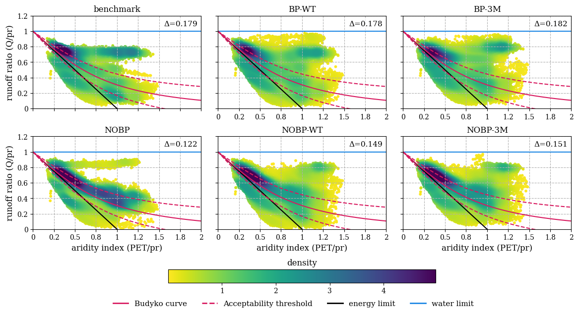
Figure 7 Density plot of aridity index vs. runoff/P. The blue line represent the water limit, where runoff < precipitation, the black line is the energy limit, derived from the relation PET ≥ AET, hence runoff/Pr ≥ 1 − PET/Pr. On the top right corner of each plot the average distance (adimensional) of each pixel from the Budyko curve is indicated.

3.4.2 Runoff

In a similar way we compare total runoff from LISFLOOD and the Budyko relationship (Fig. 7). Also in this case the original setup excluding the ByPass (NOBP) shows the highest compliance with the Budyko framework, with the highest density of points close to the Budyko curve (mean distance equal to 0.122). The other experiments perform in a similar way, with a higher density of pixels close to the Budyko curve in the most energy limited part of the plot, and spreading out towards the water limited side of the plot. The setups with active ByPass have more of a scattered behaviour than the no-ByPass experiments, with the mean distance from Budyko being higher in all cases. It is possible to distinguish high density concentration of points close and parallel to the water limit in all experiments but in particular in the benchmark, denoting that there are grid-cells where runoff is significantly higher than what suggested by the Budyko framework.

In all experiments, many grid-cells cross the energy limit (black line); assuming that PET and precipitation data is correct, runoff ought to be above the energy limit threshold, causes of this behaviour are linked to a overestimation of Precipitation, an overestimation of Q, and/or an underestimation PET. Otherwise this behaviour occurs mostly in leaky catchments (Andréassian and Perrin, 2012), so where water contributes to the replenish of the aquifer. Pixels that cross the energy limit and where the runoff is lower than the expected Budyko runoff are the red/negative values in Fig. B15. We can observe that in most of those catchments, the GwLoss parameter (Fig. B10) is close to 1, flagging the tendency of the model in storing water in the deep aquifer, at the same time in some west catchments, the bias (Fig. B3) remains positive which could lead to an hypothesis of overestimation in precipitation. When the bias is negative, the hypothesis is that the model tends to move water to the deep aquifer in order to maximize KGE.

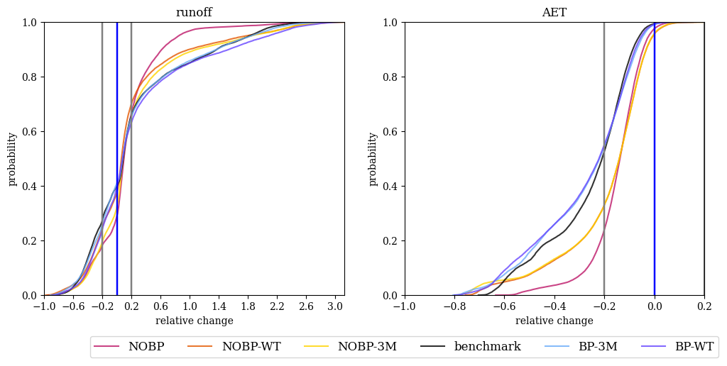
Figure 8 Cumulative Distribution Function (CDF) of the Budyko Distance (BD) calculated for each pixel of the Po river basin for total runoff (left panel), and actual evapotranspiration (right panel). The ideal value of null BD (solid blue vertical line) corresponds to a perfectly consistent model long-term partitioning of Pr between Q and AET with the expected Budyko relationship, while results of BD between −0.2 and 0.2 are considered acceptable (grey vertical lines). A few negative and positive outlier values have been removed.

On the other hand positive values in Fig. B15 mean that the runoff is higher than the one expected by the Budyko equation (points that are above the red line in Fig. 7). Generally most of the catchments in the floodplain tend to show this behaviour, with many of them showing a negative bias (Fig. B3), which could be due to an underestimation of precipitation and the model tendency to transform precipitation in runoff only in order to match observed discharge and/or a compensation of low upstream discharge entering the catchment.

The setup with no ByPass and original soil depth (NOBP) show smaller discrepancies throughout the basin. This is particularly clear from the CDFs (Fig. 8) as the NOBP experiment is the one with the narrowest dispersion around the ideal value (BD = 0). The second best performing experiments are the remaining 2 without the ByPass (NOBP-WT and NOBP-3M) which show almost identical distributions of BP. The ByPass experiments have more than 60 % analysed area exceeding 20 % (0.2 in Fig. B15) of the acceptable range. Runoff is compliant in less than 60 % of the pixels, with the experiments without ByPass performing slightly better compared to the ones with the ByPass.

3.4.3 Parameters interplay

The distributions of the Budyko Distance of AET (e.g., Fig. B14) suggest an intuitive relationship between soil depth, AET and calibrated parameters bInfilt and PowerPrefFlow (Figs. B8 and B9). Indeed, significant (Pearson's) correlation values are found between BD and several analysed parameters (Fig. 9): bInfilt, PowerPrefFlow, average sd3 and average sd2 per catchment, versus the average relative difference from Budyko AET for each catchment. Only catchments with over 30 % valid pixels (showed in Fig. A2) were included in the analysis.

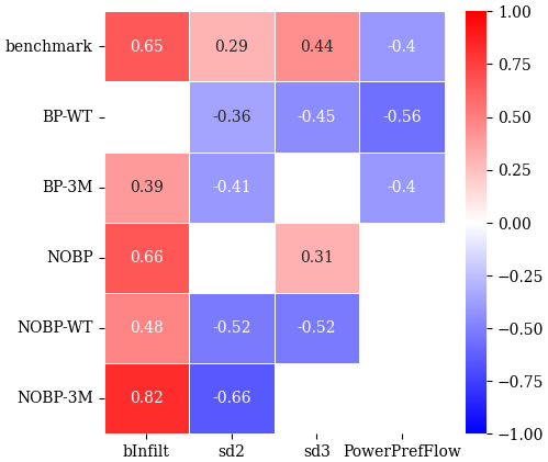
Figure 9 Correlation between Budyko Distance and parameter value (for parameters bInfilt, sd2, sd3, PowerPrefFlow). Cells are coloured only when the correlation is significant (p<0.05).

The bInfilt parameter (exponent for infiltration capacity of the soil) shows consistent positive correlation with BD across all experiments, but BP-WT, indicating that as bInfilt increases, the difference between modelled AET and Budyko AET also increases. This suggests that infiltration capacity plays a key role in shaping the deviation from the Budyko curve.

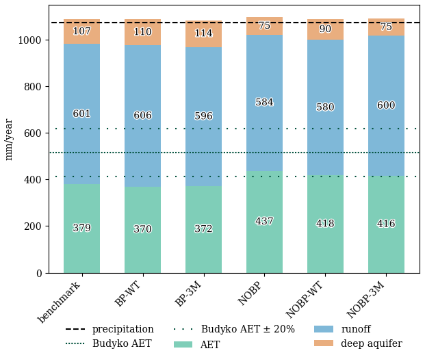
Figure 10 Water balance components (in mm yr⁻¹) for all experiments, with bars showing the partitioning of water into runoff, AET and GwLoss (deep aquifer recharge). The horizontal black dashed line represents the observed precipitation, while the dark green densely dotted line represents Budyko-estimated AET (from Eq. 14), and the dark green loosely dotted lines represent the acceptability range of ±20 %.

The sd2 parameter (depth of the second soil layer) shows a weak-moderate negative correlation in all experiments except NOBP, with the strongest inverse relationships in experiments without the ByPass mechanism. This implies that shallower soil layers (lower sd2 values) are associated with reduced AET, highlighting the importance of soil depth in AET. At the same time the lack of significance in the correlation between sd2 and NOBP, shows that without the ByPass mechanism and with a thick sd2 the BD is detangled from the sd2 value.

For sd3 (depth of the third soil layer), a weak positive correlation appears in the NOBP and benchmark experiments – where sd3 values tend to be higher (Fig. 2). In contrast, experiments with thinner sd3 layers exhibit moderate to weak negative correlations. These findings suggest that, although sd3 is not explicitly used in the AET calculation in LISFLOOD, its magnitude appears to influence AET outcomes.

The PowerPrefFlow parameter demonstrates a weak to moderate negative correlation. Notably, in the BP-WT experiment, PowerPrefFlow shows a stronger inverse correlation than bInfilt, suggesting that the ByPass mechanism does influence the AET dynamics, more than sd2 parameter.

3.5 Water balance closure

Figure 10 shows the sum of AET, total runoff and the groundwater loss expressed in mm yr⁻¹. Observed precipitation, which is equivalent in all experiments, is slightly lower than the sum of the 3 modelled components, which means that in all experiments there is more water leaving the system than water entering it. The sum of the three components (AET, Q and groundwater loss) is similar in all experiments, however the actual evapotranspiration is higher in the experiments without the ByPass (with an average increase of around 15 % with respect to corresponding experiments with ByPass). On the other hand the groundwater loss is higher in the experiments with the ByPass (with an average increase of more than 20 %). Across all experiments, the maximum AET (NOBP) is 437 mm yr⁻¹, which lies within the Budyko acceptability range, and is ≈18 % higher than the minimum one of 370 mm yr⁻¹ (BP-WT), which falls well below the acceptability range. The highest deep aquifer volume is found in the experiments with the ByPass, where the water moving to the deep aquifer is between 22 % and 52 % higher than in the experiments without the ByPass.

4 Discussion

The calibration of six alternative setups of LISFLOOD has highlighted that the original model setup, with the ByPass mechanism enabled, remains the best performing one in terms of overall streamflow accuracy (KGE and its components). Among the ByPass-enabled setups (benchmark, BP-WT, BP-3M) performance differences are minimal, regardless of the assumptions made on soil depth. The ByPass reduces the influence of the soil depth, compared to the experiments without the ByPass (NOBP, NOBP-WT, NOBP-3M), by conveying water directly to the upper groundwater zone of the model. This mechanism can prevent water from infiltrating in the unsaturated zone, causing lower evapotranspiration (AET) and influencing the accumulation of water in the deep aquifer (Fig. 1). We can argue that the ByPass shifts the water balance towards infiltration in the deep aquifer at the cost of evapotranspiration. As this may cause excessive return flow from the lower zone to the streams, the model calibration tends to elicit a higher percolation in the deep aquifer (GwLoss parameter), meaning that larger volumes of water are taken out of the system (Fig. 10). While useful to improve general-purpose streamflow accuracy (e.g., KGE), the spurious increase in groundwater losses is purely empirical and driven solely by streamflow observations (via calibration), flagging a surrender by the model in quantifying certain shares of the water balance in a physically-consistent way. Conversely, model setups excluding the process of ByPass do not offer sufficient flexibility to achieve the same performance levels (e.g., KGE). However, these setups show a similar ability to the ByPass experiments in reproducing average runoff (%BiasRR in Fig. 4) and a higher compliance with the Budyko functional relationship, which we may argue is equivalent to a more realistic response in terms of the overall water balance of the river basin; this is a case of producing the “right results for the right reasons” (Beven, 2018), where model fluxes and states better align with theoretical expectations (as observations are not available for some variables) which might lead to more robust performance under non-stationary or changed conditions (Beven et al., 2022). The prominent influence of the calibrated parameters over the physical condition is apparent from Fig. B15 where the pattern of the Budyko distance outlines the pattern of the sub-catchments instead of the natural characteristic that can affect the deviation from the Budyko theoretical relationship. Snow, for example, is known for its influence in the runoff/evaporation ratio, favouring runoff and decreasing evaporation losses. When we compare streamflow, while the individual high-flow events (e.g., at daily resolution) are better captured by the benchmark, the monthly and annual flows are predicted by the model with and without preferential flow in a comparable way, particularly in the experiment with the shallowest soil (NOBP-3M). For low-flows, both types of setups show comparable performance, indicating that the different model configurations tested are not able to improve the reproduction of low flows. We can argue that this result can be a combined effect of the high model flexibility together with the objective function used for calibration (KGE), which tends to favour accuracy on high flows rather than low flows or other regimes (Mizukami et al., 2019; Gauch et al., 2023).

The ByPass mechanism represents the well-known hydrological process known as preferential flow, which refers to fast water movement through the soil matrix (Clothier et al., 2008), travelling along specific pathways deep into the subsurface, often below the root zone. Recent studies (e.g., Kocian and Mohanty, 2024) have also highlighted how seasonality and soil properties influence the occurrence of preferential flow events.

Given its localized and heterogeneous nature, it becomes challenging to model preferential flow, especially in large scale semi-distributed models, which rely on averaged parameters over large areas. In the case of LISFLOOD, the PowerPrefFlow parameter (i.e., exponent in the preferential flow function) is homogeneously applied in each calibrated sub-catchment, removing localized and temporal effects, but also contributing to dry soil and low AET together with other model parameters. Our analysis (Fig. 9) indicates that there is an interplay between PowerPrefFlow, saturation excess (bInfilt), and soil depths for the estimation of AET. Soil depth plays a more prominent role in the experiments without ByPass and for sd2 values thinner than 1 m (as in WT and 3M experiments); on the other hand, in the ByPass experiments, the PowerPref flow becomes more important than soil depth in reducing AET from the expected Budyko value. Moreover, the stream network parameters controlling water transfer speed and correlation are less important in the setups including the ByPass (Fig. 5), because the PowerPrefFlow parameter strongly controls the quantity and timing of fast/subsurface runoff, influencing the flow timing more than the parameters that describe channel properties. These findings reinforce our argument that the ByPass and the Xinanjiang-VIC-Arno components, as currently parametrized, can uncontrollably lead to diminish the hydrological realism of the water balance, while adding flexibility and improving accuracy on high-flow events.

The moderate-high correlation between saturation excess (bInfilt) and the relative difference from the Budyko AET (Fig. 9), indicates that limiting the upper bound of saturation excess (bInfilt, currently between 0.1–5) could improve the representation of AET by forcing water to infiltrate in the vadose zone and hence make it available to plants transpiration. When calibrating with a lower saturation excess (bInfilt), the PowerPrefFlow would have to automatically adjust to find the best combination of parameters leading to the best performance. However, this parameter compensation process should be carefully evaluated, since some performance metrics (e.g., KGE) may significantly deteriorate under these conditions, highlighting trade-offs between overall performance metrics and internal consistency of water balance components, as demonstrated in this study. Adding constraints on saturation-excess parameters (bInfilt) would make the role of soil depth more prominent, as the AET and KGE results show in the experiment without the ByPass. Shallower soil depth leads to lower AET and a minimum depth of 1 m seems to ensure a correct AET estimation if saturation excess (bInfilt) and PowerPrefFlow are correctly parametrized. That is supported by the AET performance in the NOBP and the benchmark that show a good Budyko compliance, unless when saturation excess (bInfilt) is above 4 (Fig. 6).

Changing the soil depth has shown to help improve the KGE performance in the NOBP-3M setup, which excluded the ByPass. In particular, the third soil layer of the model is assumed to not contribute to AET, and works only as a buffer between the unsaturated zone and the upper groundwater zone. In the experiments without ByPass, a deeper soil delays the transfer of water and contributes to a lower performance. Shallower soils allow water to move faster to the upper groundwater zone, from where it contributes to subsurface runoff. These findings suggest that a way to enhance Budyko compliance without compromising streamflow performance (KGE) could be by constraining saturation excess (bInfilt) and adjusting the third soil depth. While including sd3 in the calibration process could further improve model results, it also increases the risk of over-parametrization, potentially leading to unexpected or unreliable outcomes. Careful consideration is therefore needed when expanding and/or constraining the parameter set and/or modifying the preferential flow process.

The aforementioned considerations highlight the need for a deeper investigation of how the LISFLOOD model simulates the vadose zone, identifying which processes should be constrained or structurally modified to ensure that the model achieves the right response (streamflow) for the right reasons, that is, with internally consistent states and fluxes (Beven and Cloke, 2012; Wagener and Pianosi, 2019). If internal fluxes deviate too much from physically plausible bounds and theoretical expectation, the model is producing the right output (streamflow) for the wrong reasons, and the modeller has no principled way of knowing whether the model will remain reliable under non-stationary conditions, in ungauged basins, or for any application beyond the calibration target.

We argue that this structural diagnosis should precede, rather than be replaced by, the introduction of additional calibration targets, whether in the form of extra parameters to be calibrated or of external constraints such as ET or Budyko-based metrics added to the objective function. With the rapid advances in deep-learning approaches in hydrology, this finding raises a more pressing question: if a black-box model can predict the target variable as well as or better than a physically based one, the value of the physical model rests precisely on its internal realism. Audits like the one we present, in our view, are the way to defend (or challenge) that value. Conversely, when a physically based model is set up correctly, internal-realism diagnostics are informative on their own. A model run on a leaky catchment, with poor-quality forcing, or with a missing process (e.g., unmodelled irrigation), should fail the diagnostic check. Rather than masking such issues through compensatory calibration, the failure itself is useful information, pointing the modeller toward data quality issues, incorrect parametrisation, structural gaps, or lack of process understanding (Blöschl, 2026). In such cases, a deep-learning model trained to reproduce streamflow may perform its intended task well, but cannot provide the same diagnostic information on data quality or process representation that a well-constrained physically based model can.

We highlight two complementary ways forward from our analysis. The first one, in line with the arguments on defensible model complexity of Guthke (2017), would be to simplify the representation of the vadose zone in LISFLOOD. Our results show that the evapotranspiration equations are sensitive to the soil depth and to the amount of water allowed to infiltrate. The currently allowed parameter ranges of soil depth, preferential flow and infiltration (bInfilt), together with the AET equations used in LISFLOOD, can lead to unrealistic estimates of AET. Reducing the number of interdependent parameters governing AET, runoff, and infiltration, for which large-scale, good-quality observations are limited anyway, would probably yield a more robust representation of the main fluxes and states of the water balance, which could be validated against long-term Budyko AET.

The second one is to apply Global Sensitivity Analysis (GSA) for guiding hydrological model development and quantifying the influence of modelling choices (Wagener and Pianosi, 2019). Past sensitivity and uncertainty analyses on LISFLOOD focused solely on streamflow (Zajac et al., 2017; Bisselink et al., 2016; Feyen et al., 2008); extending the scope to internal fluxes and states would inform how different parameters influence various processes and their interactions, and would help identify which structural simplifications are most defensible. To achieve robust sensitivity estimates, GSA typically requires a large number of model runs (Wagener and Pianosi, 2019), which is computationally demanding for (semi-)distributed hydrological models. Here the two directions reinforce each other: a simplified model with fewer interdependent parameters is also a more tractable target for systematic sensitivity analysis, and the analysis itself can guide which simplifications preserve the diagnostically relevant model behaviour. Moreover, incorporating spatially distributed Earth Observation (EO) products, such as soil moisture and evapotranspiration (ET) data, into the diagnostic framework would complement the theoretical Budyko-based diagnostic with observation-based evidence, supporting the identification of structural inadequacies at the grid-cell level and guiding model development toward more realistic representations of AET and other internal hydrological processes. The Po basin itself has been the subject of an EO-based reconstruction of the water cycle (Brocca et al., 2024).

Another aspect to consider is the general design of the LISFLOOD model, which implicitly incorporates human influences by using non-naturalized streamflow time series for calibration. This approach, while necessary due to the large number of calibrated stations (1903) across Europe (ECMWF, 2022) and the diversity of data sources, may introduce biases when human influences are not fully accounted for (Terrier et al., 2021). Given the general lack of knowledge of water management practices, including inter-basin transfers-information that is often unavailable, improving the explicit modelling of these influences is an open challenge. This knowledge gap, combined with the model’s calibration routine, can lead to systematic errors affecting the water balance components. For instance, in basins where water is artificially transferred from other catchments, or the flow is heavily regulated, the model may underestimate AET. This occurs because additional inflows increase streamflow, which the model may balance by reducing AET or soil water storage, thus closing the water balance at the expense of accurately representing other hydrological processes. A further concern arises from the absence of explicit groundwater-transfer processes in LISFLOOD combined with the cascading calibration approach employed for the calibration of EFAS and GLOFAS. In catchments where groundwater moves (“leaky catchments”) to neighbouring basins, the model cannot represent this transfer. During calibration, the water that is actually moved via groundwater may instead be assigned to the deep aquifer storage (gwloss). Consequently, the leaky catchment may show lower simulated runoff and/or AET (potentially below the theoretical optimum such as a Budyko curve metric), while the receiving catchment might show an overestimation – or at least a mismatch – of runoff or AET (Andréassian and Perrin, 2012).

A similar issue arises when precipitation is over- or under-estimated: if precipitation is underestimated, the model may achieve a good streamflow fit by lowering AET, if precipitation is overestimated, the model may compensate by increasing deep aquifer storage (gwloss).

In the context of LISFLOOD calibration, and more generally in semi-distributed models, the Budyko framework proves to be an effective tool for model diagnostic, for a better interpretation of model results, and verification of simulated AET. As also suggested by Gnann et al. (2023), this verification is necessary for a reliable use of model outputs that are not directly calibrated. In particular, the cell-based evaluation can help the modeller to spot deviations from the expected Budyko value. A natural next step in developing this diagnostic tool would be to classify areas a priori according to whether higher, lower, or comparable AET is expected with respect to the Budyko empirical AET. For example, in mountainous regions, karstic, or impervious areas we expect a lower AET than the Budyko value, whereas a higher AET is expected when significant water sources exist beyond precipitation (e.g., irrigation) or where the landscape features high water retention or strong groundwater influences. Combined with the four FDC-based signature metrics on streamflow, this classification can shed light on how the model partitions water among storage, AET, and runoff, and on which part of the flow-duration curve discrepancies concentrate. The evaluation of modelled fluxes and states against such functional relationships is model-agnostic and can be performed on any hydrological model, whereas the link between observed discrepancies and the underlying model structure or parameters is necessarily model-specific. This separation between general diagnostics and model-specific interpretation aligns with the broader perspective advocated by Gleeson et al. (2021) and Gnann et al. (2023), and is, in our view, the natural direction in which our work can be extended.

Recent studies have moved in this direction. For example, Wang et al. (2026) introduce an event-type-based multi-dimensional diagnostic framework that evaluates timing and magnitude errors for streamflow events of different types (e.g., snow-related events, rainfall on dry or wet soils) and uses explainable machine learning to identify the relative importance of different sources of error, providing a route to diagnose which processes drive event-type-specific model failures. While Wang et al. (2026) focus on streamflow events, our diagnostic considers both long-term streamflow and AET against the Budyko expectation; combining the two perspectives, event-scale streamflow diagnostics and long-term flux-based diagnostics, could provide a more complete picture of where and why a model fails.

Beyond diagnostics, another way to include the Budyko framework, and the BD, could be employed in the constraining of the parameter space prior calibration, ensuring that only physically meaningful values are considered. Alternatively, it can be integrated as a metric during calibration or used in post-calibration evaluation to guide parameter selection/tuning, reducing equifinality, and identify combinations that underestimate AET.

However, care must be taken when applying the Budyko relationship as an objective function in a multi- or single-objective calibration, particularly in catchments heavily influenced by human activities or that underwent significant land-use changes that are not accounted for in the model. In such cases, the theoretically expected partitioning between runoff and AET may not hold, and enforcing Budyko constraints could lead to suboptimal or unexpected results.

5 Conclusions

We have examined how the LISFLOOD hydrological model reproduces the water balance components across six setups on the representative case-study of the Po river basin in Northern Italy. We have shown that the setup with the preferential flow (ByPass) mechanism currently implemented in EFAS v.5.0 outperforms the tested alternative setups without the ByPass in terms of streamflow accuracy (based on the KGE and its components). However, this owes to a large extent to the inclusion of a preferential flow process, which can cause underestimation of infiltration in soils and of actual evapotranspiration, as well as a consequent overestimation of recharge to aquifers. To compensate, the model relies on an empirical parameter to adjust groundwater losses, which retains limited physical meaning and may limit the validity of the model when addressing water resources management questions beyond streamflow (e.g. aquifer recharge, estimation of irrigation requirements and availability of groundwater resources). The deviations between the modelled water balance components and Budyko-based predictions are particularly apparent when the second soil layer is shallow (<1 m) and for low values and high values of PowerPrefFlow and bInfilt respectively.

Further research is needed to understand how to improve the model and/or constrain parameters to keep a good performance in terms of KGE and an acceptable representation of AET and groundwater components. Experiments excluding the preferential flow show a higher consistency with the Budyko framework, but lower accuracy (KGE) against observed streamflow at daily time step. However, aggregated streamflow volumes at monthly and yearly scale, as well as low flows at daily step are predicted with accuracy comparable with the setups with preferential flow. While a performance metric targeting the goodness-of-fit of daily observed and simulated streamflows (e.g., KGE) is key when considering flood applications, a plausible representation of soil moisture, evapotranspiration and groundwater dynamics is also essential for water resources management and climate adaptation. The diagnostic workflow we applied is model-agnostic and transferable to other distributed models, even where the link between a detected discrepancy and its structural cause remains model-specific. We argue that this kind of auditing is becoming more rather than less important: as data-driven models match or exceed physically based ones on streamflow, the distinctive value of a physical model lies in the internal, physically-consistent water-balance information it provides. A diagnostic failure becomes then itself informative, pointing to forcing errors, parametrization, or missing processes. Auditing of the kind presented here is, in our view, how that value of physically-models is defended or challenged.

Appendix A: Calibrated parameters and study area

Study area (Fig. A1) and model cells used in the Budyko analysis (Fig. A2)

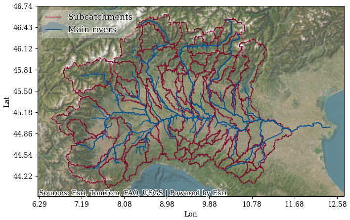
Figure A1 Study area, the Po river basin, with the 60 calibrated sub-catchments (boundaries in dark red) and the main rivers (dark blue lines). Satellite background was retried from Esri (n.d.). World Imagery, https://www.arcgis.com/home/item.html?id=10df2279f9684e4a9f6a7f08febac2a9 (last access: 10 May 2026) | Powered by Esri.

Figure A2 Model domain, showing cells included in the AET/Budyko analysis and the water balance diagnostics (Fig. 10) in grey (the white area was excluded due to land cover criteria detailed in Sect. 2.5.2).

Table A1 LISFLOOD model parameters subject to calibration (ECMWF, 2022).

Appendix B: Results

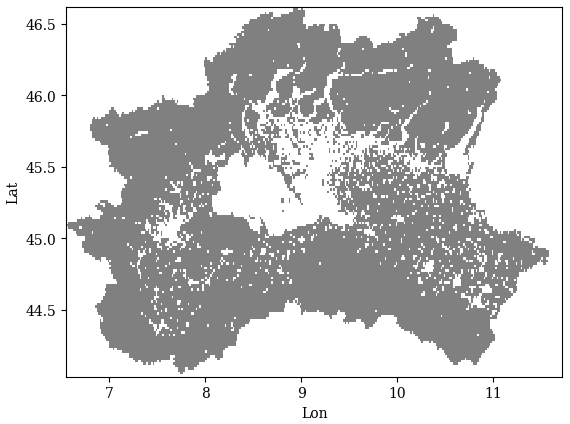
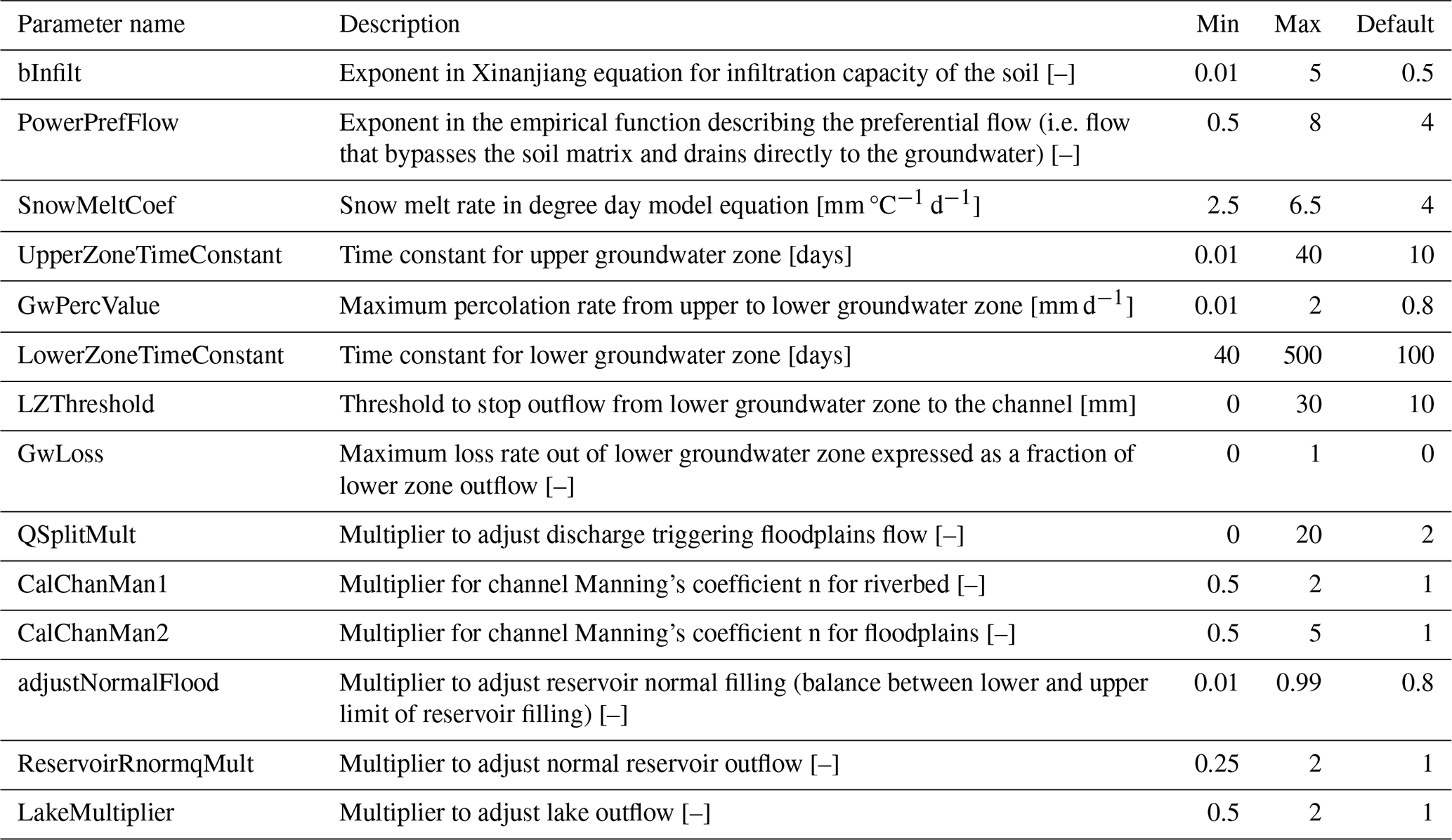
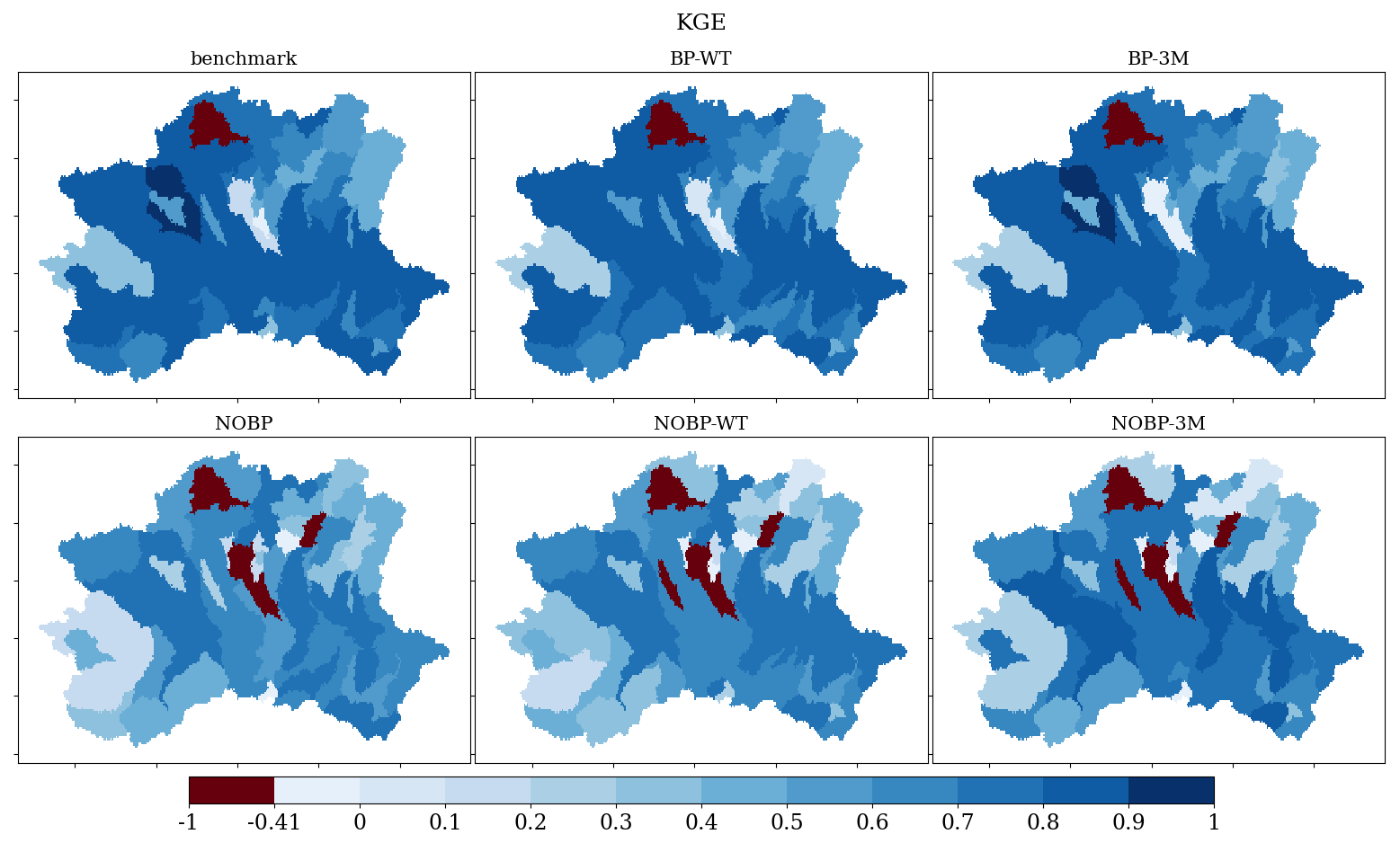
Figure B1 KGE for all the calibrated sub-catchments in all the 6 experiments (the optimal value for KGE is 1).

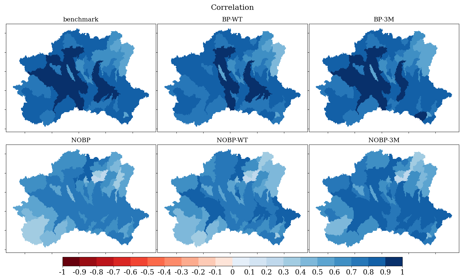
Figure B2 Correlation for all the calibrated sub-catchments in all the 6 experiments (optimal value is 1).

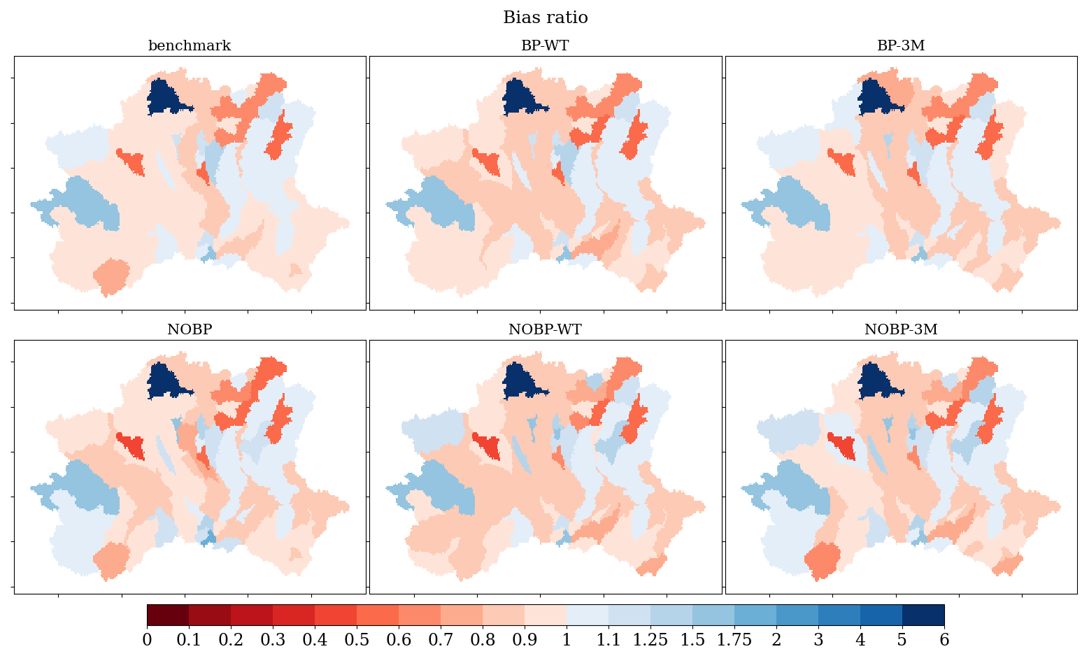
Figure B3 Bias ratio for all the calibrated sub-catchments in all the 6 experiments (optimal value is 1).

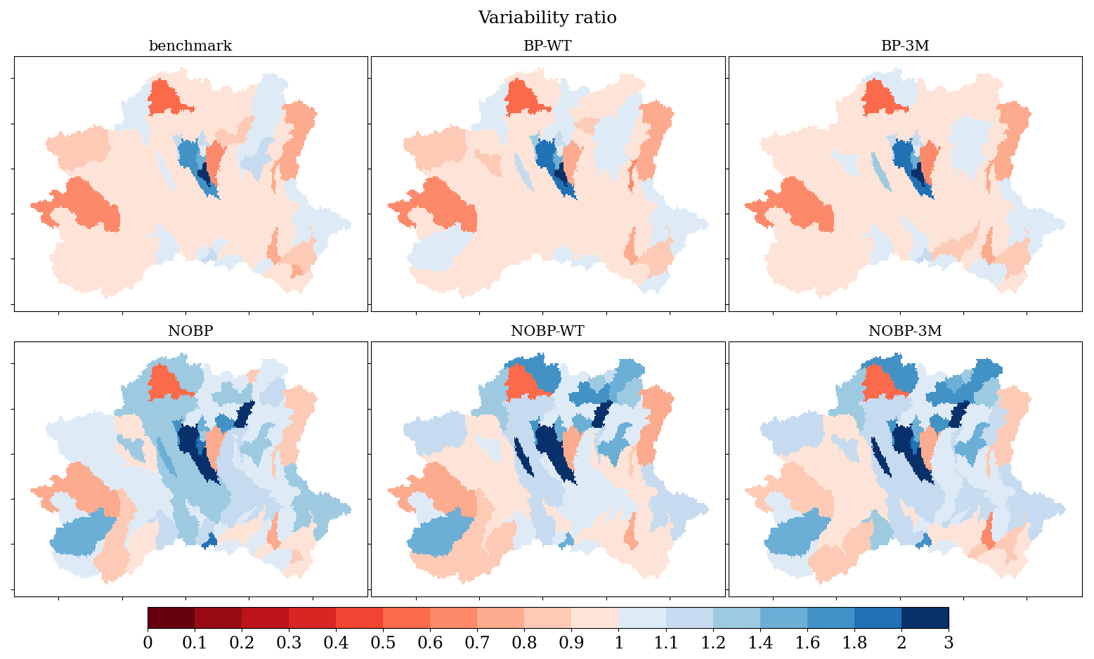
Figure B4 Variability ratio for all the calibrated sub-catchments in all the 6 experiments (optimal values is 1).

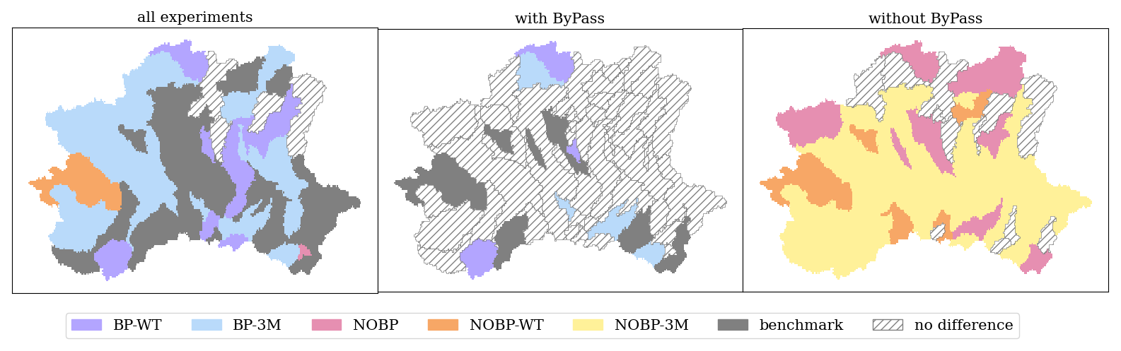
Figure B5 Best performing setup in terms of KGE (at daily scale) across sub-catchments, considering all the experiments (left panel), the subset of experiments with ByPass (middle panel), and without ByPass (right panel). When the difference of KGE among all the experiments is below 0.05, the performance of all setups is comparable (we define it as “no difference”) and the sub-catchment area is filled with oblique grey lines.

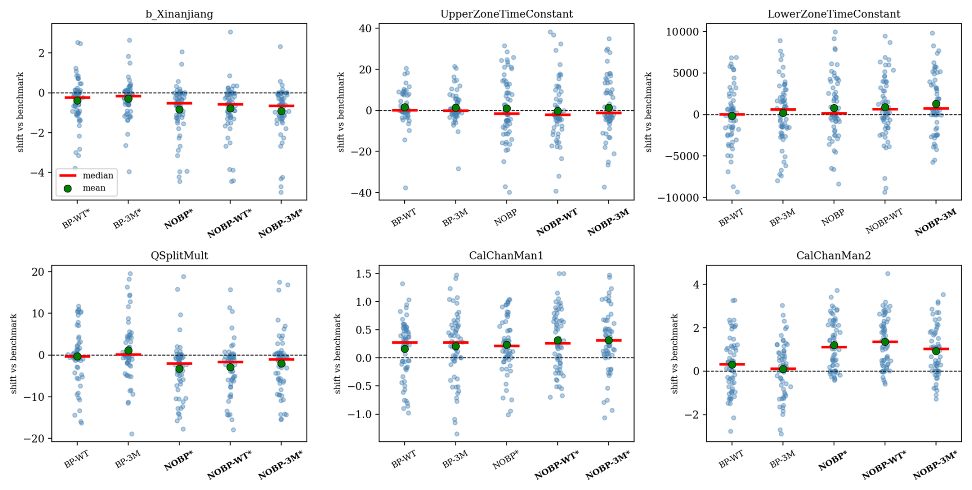
Figure B6 Distribution of paired shifts in calibrated parameters (alternative setup – benchmark configuration) across the sub-catchments for the six parameters where at least one alternative differs significantly from the benchmark under at least one of the two statistical tests (KS and WD-based test with BH correction).

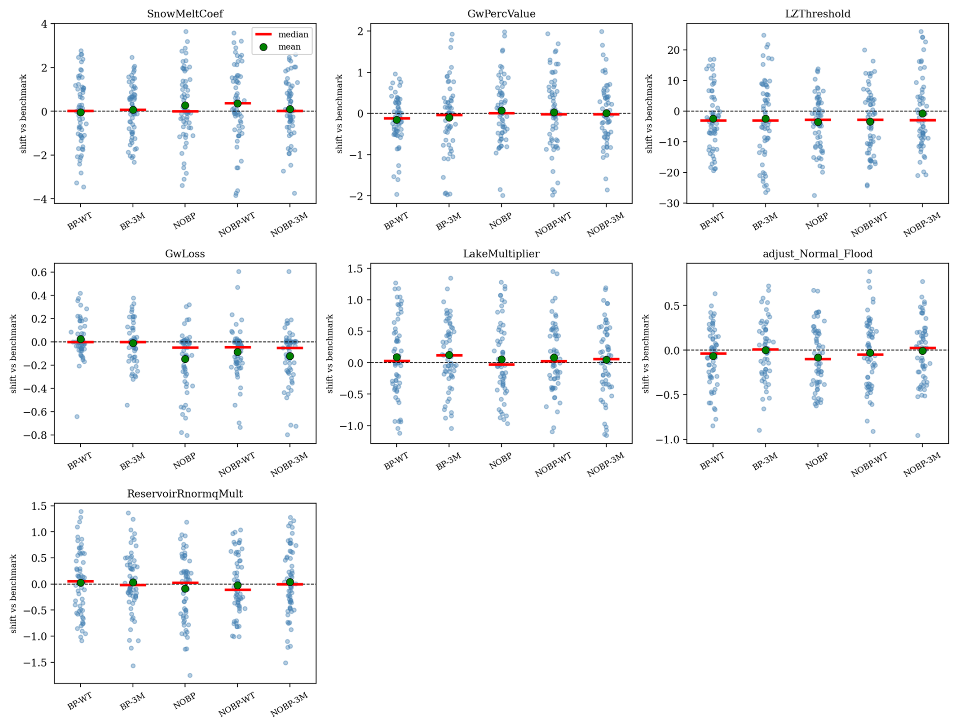
Figure B7 Distribution of paired shifts in calibrated parameters (alternative setup – benchmark configuration) across the sub-catchments for the seven parameters where no significant differences are detected by either statistical test (KS and WD-based test with BH correction) between any setups with respect to the benchmark of the two statistical tests.

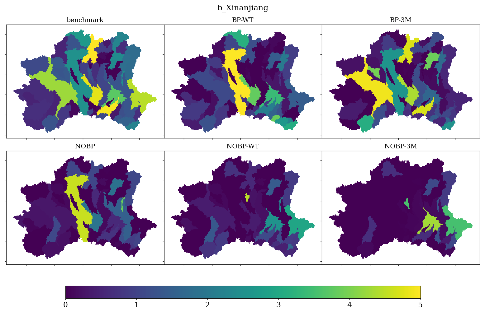
Figure B8 Calibrated parameter bInfilt for each experiment setup.

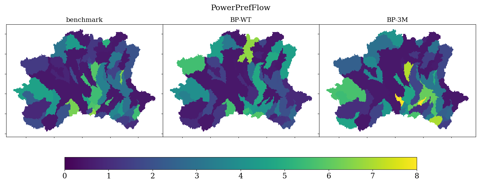
Figure B9 Calibrated parameter PowerPrefFlow for each experiment setup. The parameter was not used for the experiments without ByPass.

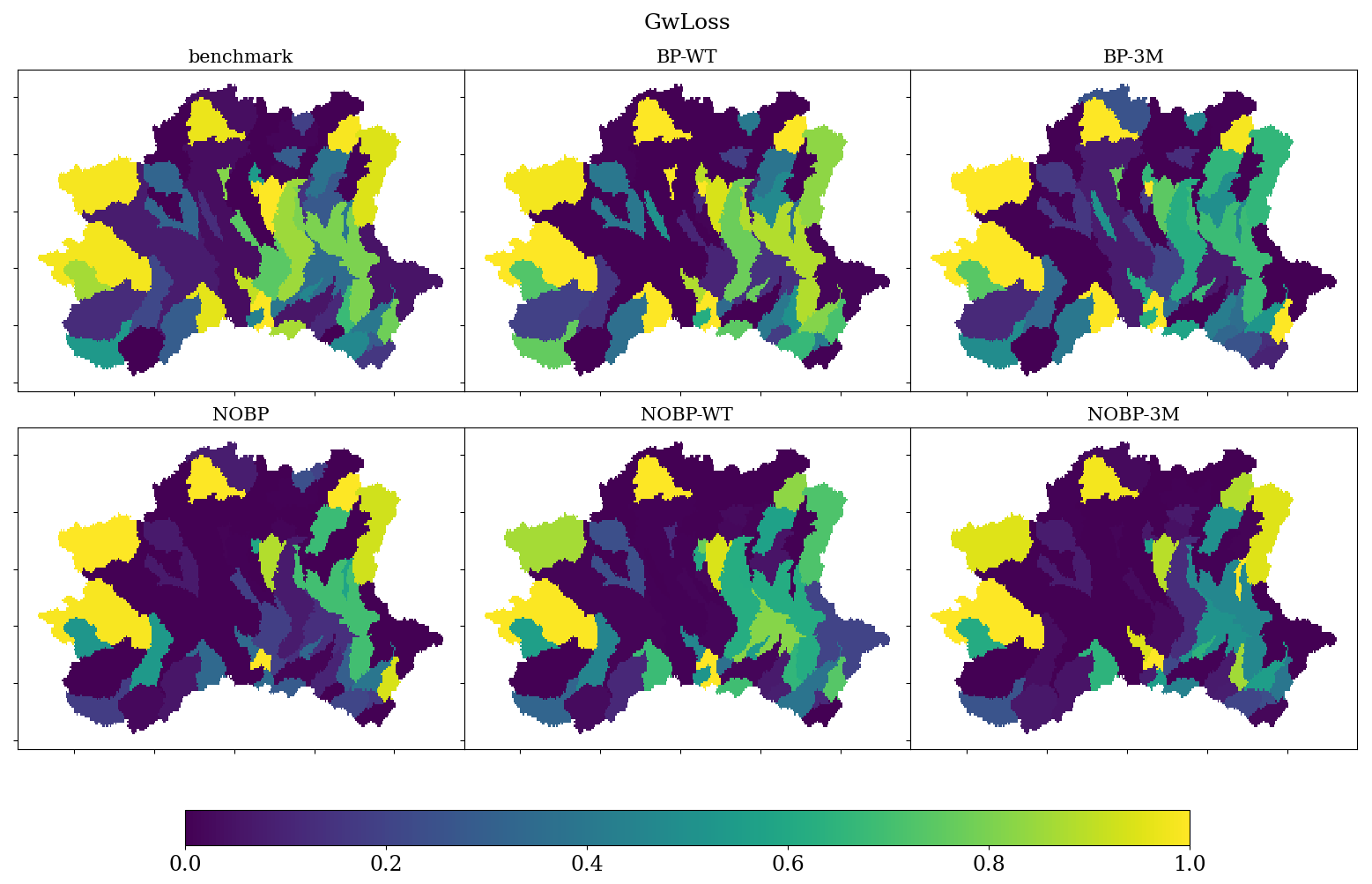
Figure B10 Calibrated parameter GwLoss for each experiment setup.

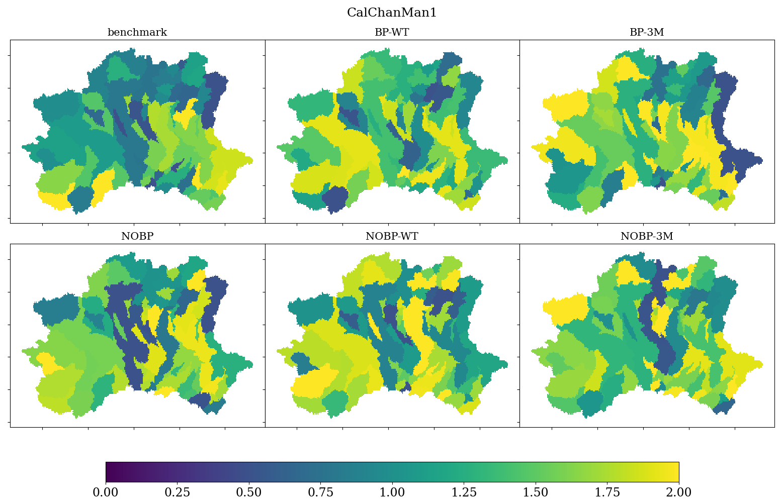
Figure B11 Calibrated parameter CalChanMan1 for each experiment setup.

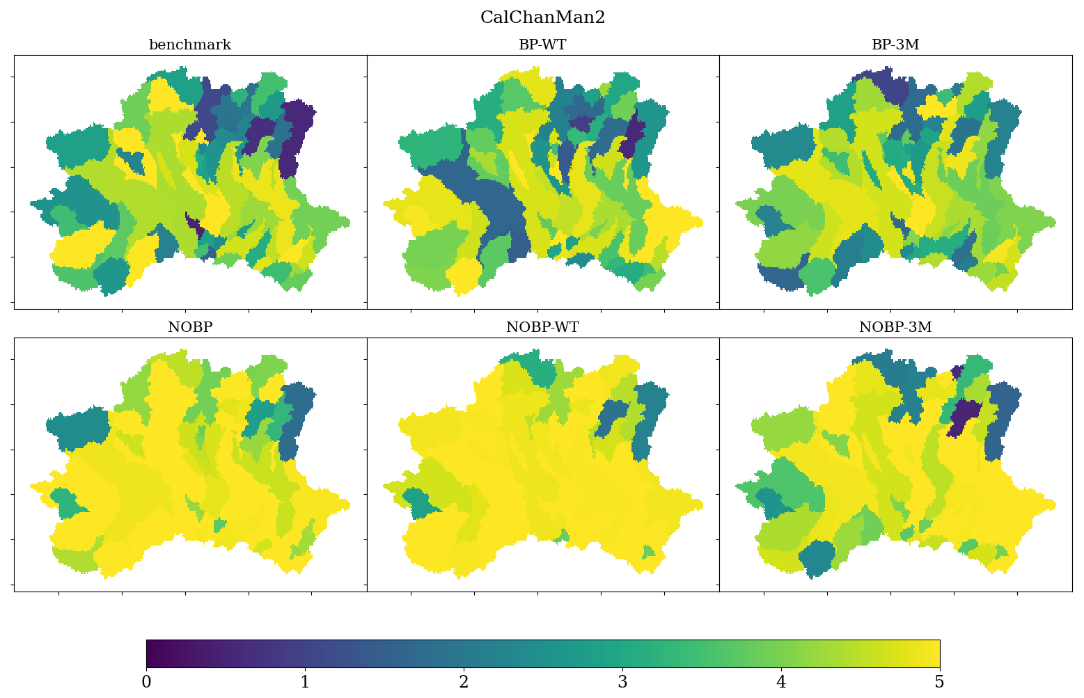
Figure B12 Calibrated parameter CalChanMan2 for each experiment setup.

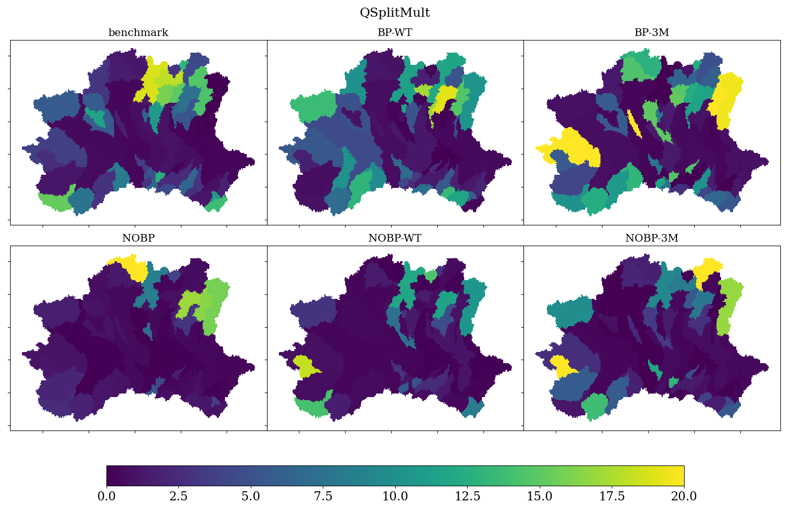
Figure B13 Calibrated parameter QSplitMult for each experiment setup.

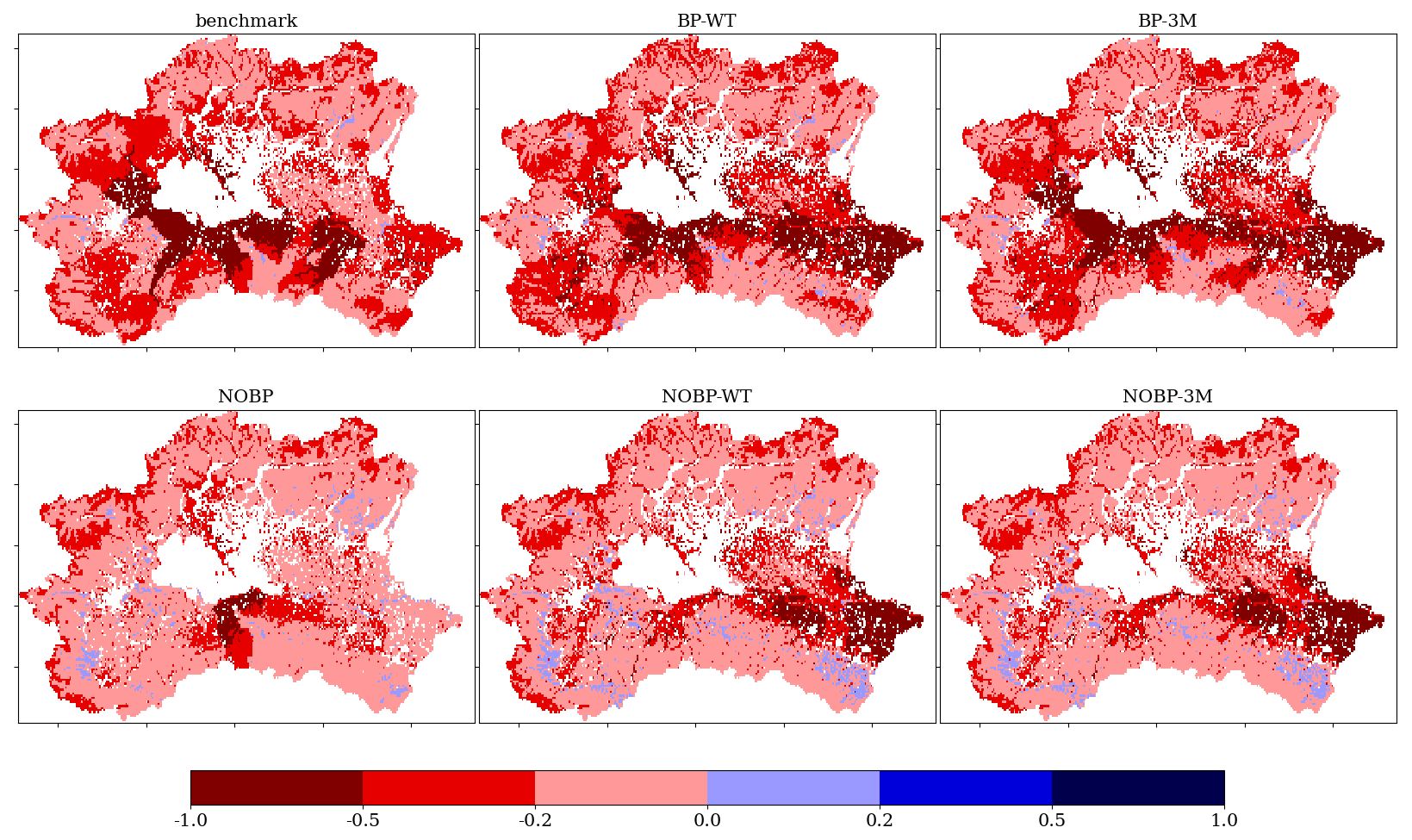
Figure B14 Relative difference of modelled annual average AET from the expected Budyko AET per pixel. Negative values (represented in red) mean that the modelled AET is lower compared to AET calculated using Budyko, while positive values (blue) mean that AET is higher compared to Budyko.

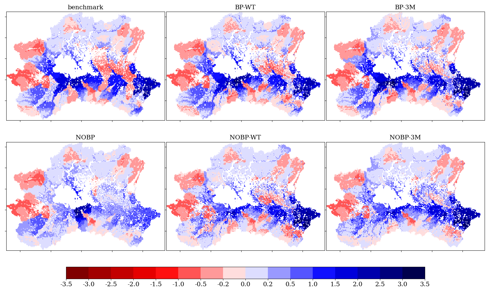
Figure B15 Relative difference of modelled annual average runoff (P − AET) from the expected Budyko runoff per pixel. Negative values (represented in red) mean that the modelled runoff is lower compared to runoff calculated using Budyko. Positive values (represented in blue) mean that the modelled runoff is higher compared to the runoff calculated using the Budyko equation.