Grounding-line dynamics in a Stokes ice-flow model (Elmer/Ice v9.0): improved numerical stability allows larger time steps

The efficient and accurate simulation of grounding line dynamics in marine ice-sheet models remains a challenge, largely due to restrictive time-step limitations. The restrictive time step size of ice-sheet simulations ($\sim \mathrm{\Delta }t=\mathrm{0.01}-\mathrm{0.5}$ years) is one of the reasons for the routine use of approximate models that compromise physical complexity compared to full Stokes models. To address the time-step restriction and enhance the applicability of full Stokes simulations, we implement a numerical stabilisation scheme at the ice–ocean interface, namely the Free-Surface Stabilisation Algorithm (FSSA). The FSSA acts by predicting the surface elevation at the next time step, resulting in a reduction in surface oscillations and an increase in the largest numerically stable time step. When applied to the ice–ocean interface, FSSA acts in combination with the sea spring numerical stabilisation scheme, allowing larger time steps to be taken.

In order to test the capabilities of the FSSA when applied to the ice–ocean interface, we perform the benchmark simulation of Experiment 3a from the Marine Ice Sheet Model Intercomparison Project (MISMIP). These simulations demonstrate the ability of the model to capture grounding line migration on both prograde slopes (oceanward sloping) and retrograde slopes (inland sloping). We find a time step size of Δt=10 years to be numerically stable and accurate in the MISMIP experiment, which is more than an order of magnitude larger than the small time steps traditionally used. In comparison, a time-step size of Δt=50 years can maintain numerical stability, but is not capable of capturing the full range of grounding-line motion in the MISMIP experiments. We further demonstrate the applicability of the FSSA to a 3D marine terminating model domain of Ekström Ice Shelf, finding that a time-step size of Δt=10 years is numerically stable. However, these results are obtained for relatively slowly evolving grounding-line dynamics, and caution is required for more rapidly evolving systems driven by ocean melting (e.g., Thwaites Glacier). The increase in the largest numerically stable time step by greater than an order of magnitude in marine-terminating Stokes ice-flow problems through the inclusion of FSSA broadens the applicability of Stokes models, which have otherwise been deemed too computationally expensive for large-scale applications.

1 Introduction

The Antarctic and Greenland Ice Sheets collectively hold an ice volume with a sea-level equivalent of 65.3 m (Morlighem et al., 2017, 2020). The loss of ice from these two remaining ice sheets has the potential to significantly influence global sea level, but projection uncertainties persist due to model variability (Fox-Kemper et al., 2021). The mass balance of the coastal regions of ice sheets is particularly susceptible to changes in accumulation and melt (Donat-Magnin et al., 2021; Višnjević et al., 2025). Furthermore, these regions are characterised by complex flow dynamics at the grounding line, where the ice transitions from grounded to floating. The ability to accurately capture grounding-line dynamics in ice-sheet models is particularly important because a retreating or advancing grounding line induces a change in ice volume and influences the sea level. Furthermore, when the bed slopes inland, the grounding line can be subject to the marine ice-sheet instability (MISI, Schoof, 2007) and competing mechanisms such as accumulation-elevation feedbacks (Sergienko, 2022; Sergienko and Haseloff, 2023).

It has been recognised that the mesh resolution at the grounding line has an influence on its dynamic evolution in ice sheet models (Durand et al., 2009b; Williams et al., 2025). Many studies have implemented an adaptive mesh algorithm to allow simulations to be performed with a high resolution at the grounding line and a coarser resolution elsewhere (Durand et al., 2009b; Goldberg et al., 2009; Gladstone et al., 2010, 2012; Gagliardini et al., 2016; Dos Santos et al., 2019). However, such high resolutions are not feasible in continental-scale simulations, so alternative approaches have been developed. These include sub-grid methods (Cheng et al., 2020) or reduced-order modelling (Larour et al., 2012; Seroussi et al., 2014).

The modelling of ice flow in coastal regions is particularly challenging because high-complexity, high-resolution nonlinear Stokes models are needed for accuracy (Rückamp et al., 2022). Since such models require significant computational resources, lower-order approximate models are predominantly used for continental-scale simulations. Only a small number of ice-sheet codes support the use of a full nonlinear Stokes solver for transient marine ice-sheet modelling (e.g. Elmer/Ice; Gagliardini et al., 2013) and are regarded as benchmark models against which lower-order models are compared. However, widespread adoption of full Stokes models is hindered by their computational expense and is exacerbated by a restrictive time-step size stemming from numerical stability issues. Our work builds on many previous theoretical (Fowler, 1986; Schoof, 2005) and finite-element (Gagliardini et al., 2007; Stubblefield et al., 2021; de Diego et al., 2022) studies of contact problems in subglacial cavities and grounding-line Stokes problems. Other work also investigated the effect of the chosen friction law and grounding-line discretisation of the transition in boundary conditions (Gagliardini et al., 2016; Brondex et al., 2017, 2019). However, few studies have investigated improving the computational efficiency of full-Stokes contact problems (Durand et al., 2009a; Cheng et al., 2020).

In order to improve the numerical stability and applicability of Stokes simulations with an ice–ocean interface, we introduce the Free-Surface Stabilisation Algorithm (FSSA; Kaus et al., 2010; Löfgren et al., 2022, 2024) at the ice–ocean interface. The FSSA mimics an implicit time-stepping scheme by predicting the free surface elevation in the next time step to account for an increase or decrease in ice thickness. The FSSA improves on the previously implemented sea spring numerical stabilisation scheme (Durand et al., 2009a). FSSA was originally conceptualized by Kaus et al. (2010) for geodynamics applications. It was subsequently adapted to grounded ice sheet simulations by Löfgren et al. (2022, 2024). The FSSA has further been adapted so that the numerical stabilisation terms vanish on convergence in a framework that allows for large time steps in a fully implicit, higher-order time-stepping framework for grounded ice (Ahlkrona et al., 2026). In Westling Dolling et al. (2026) an FSSA-like stabilisation was constructed for depth-integrated Shallow Shelf Approximation models. In this paper, we present the first application of FSSA to full Stokes floating ice problems.

To analyse the efficiency and accuracy of Stokes grounding-line simulations with the inclusion of the FSSA, we perform simulations ranging from (1) a 2D marine ice-sheet domain set up with advancing and retreating phases of grounding line migration using the Marine Ice Sheet Model Intercomparison Project (MISMIP) framework (Pattyn et al., 2012), to (2) 3D simulations of Ekström Ice Shelf in Dronning Maud Land, East Antarctica. This study provides progress toward the routine use of full Stokes models in regions with complex stress regimes such as grounding-line dynamics by allowing an increase in computational efficiency due to a larger numerically-stable time step size.

The inclusion of FSSA in Stokes models of coastal regions, as demonstrated in our study, brings higher-order models closer to broad applicability. Unlike current large-scale ice-sheet models, full Stokes models do not assume hydrostatic equilibrium at the grounding line and include all stress components, allowing accurate simulation of grounding zones where the stress regimes switch from vertical-shearing dominated dynamics to horizontal stretching. While small time steps are needed for physical reasons such as rapid grounding line migration or short-term temporal variation in surface accumulation and melt rates, the speedup has significant potential during time frames when the ice geometry and velocity are close to equilibrium, such as in paleo ice-sheet simulations or in spin-up simulations (Seroussi et al., 2019).

2 Methods

In this section, we provide details of the ice-flow model, which is implemented in the finite element software Elmer/Ice (v9.0, Gagliardini et al., 2013; Ruokolainen et al., 2023).

2.1 Stokes model

Ice is a highly viscous, shear-thinning fluid, with conservation of momentum described by the Stokes equations,

$$\begin{array}{}\text{(1)}& \mathrm{\nabla }\cdot \mathit{\sigma }={\mathit{\rho }}_{\mathrm{i}}\mathit{g},\end{array}$$

where σ is the Cauchy stress tensor, ρ_i is the ice density, and $\mathit{g}=(\mathrm{0},\mathrm{0},g)$ is the gravitational acceleration. The Cauchy stress tensor can be split into pressure, p, and a deviatoric stress tensor, τ,

$$\begin{array}{}\text{(2)}& \mathit{\sigma }=\mathit{\tau }-p\mathbf{I},\end{array}$$

where I is the identity matrix. The conservation of mass is expressed as an incompressibility condition,

$$\begin{array}{}\text{(3)}& \mathrm{\nabla }\cdot \mathit{u}=\mathrm{0},\end{array}$$

where $\mathit{u}=(u_x,u_y,u_z)$ is the velocity vector. In order to relate the nonlinear response of the strain rate of ice to an applied stress, Glen's flow law is used,

$$\begin{array}{}\text{(4)}& \mathit{\tau }=\mathrm{2}\mathit{\eta }\left(\dot{\mathit{\epsilon }}\right)\dot{\mathit{\epsilon }},\end{array}$$

where $\dot{\mathit{\epsilon }}$ is the symmetric part of the velocity gradient tensor, i.e. $\dot{\mathit{\epsilon }}=\mathrm{1}/\mathrm{2}(\mathrm{\nabla }\mathit{u}+\mathrm{\nabla }{\mathit{u}}^{\mathrm{T}})$. The effective viscosity, $\mathit{\eta }=\mathit{\eta }\left(\dot{\mathit{\epsilon }}\right)$, is defined as

$$\begin{array}{}\text{(5)}& \mathit{\eta }={\displaystyle \frac{\mathrm{1}}{\mathrm{2}}}{A}^{-\mathrm{1}/n}{\left({\dot{\mathit{\epsilon }}}_{\text{crit}}^{\mathrm{2}}+{\displaystyle \frac{\mathrm{1}}{\mathrm{2}}}\left|\right|\dot{\mathit{\epsilon }}|{|}_{\mathrm{F}}^{\mathrm{2}}\right)}^{(\mathrm{1}-n)/\mathrm{2}n}.\end{array}$$

Here, the effective strain-rate, $\left|\right|\dot{\mathit{\epsilon }}|{|}_{\mathrm{F}}$, is the Frobenius norm of the strain rate tensor, which can be written $\left|\right|\dot{\mathit{\epsilon }}|{|}_{\mathrm{F}}=\sqrt{\text{tr}(\mathrm{1}/\mathrm{2}{\dot{\mathit{\epsilon }}}^{\mathrm{2}})}$. The rheological parameter, A, controls the fluidity of the ice and is spatially constant in this study, but is temporally-varying in specified simulations (Sect. 4). A regularisation term, ${\dot{\mathit{\epsilon }}}_{\text{crit}}^{\mathrm{2}}={\mathrm{10}}^{-\mathrm{15}}{\mathrm{a}}^{-\mathrm{1}}$, is included to numerically stabilise the viscosity as the strain rate approaches zero.

2.2 Stokes boundary conditions

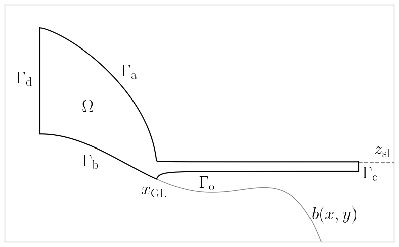
Figure 1 A schematic for the idealised 2D MISMIP Exp 3a set up. The model is also applied to a 3D, real-world ice sheet–ice shelf set up. The model domain, Ω, and the domain boundaries, $\partial \mathrm{\Omega }={\mathrm{\Gamma }}_{\mathrm{a}}\cup {\mathrm{\Gamma }}_{\mathrm{b}}\cup {\mathrm{\Gamma }}_{\mathrm{o}}\cup {\mathrm{\Gamma }}_{\mathrm{c}}\cup {\mathrm{\Gamma }}_{\mathrm{d}}$ are shown in 2D. The ice-atmosphere interface is denoted by Γ_a, the ice-bed interface by Γ_b, the ice–ocean interface by Γ_o, the calving front by Γ_c and the ice divide by Γ_d. The sea level is denoted by z_sl, the grounding-line position by x_GL and the bed elevation by b(x,y).

The Stokes equations are solved on a domain Ω, with a Cartesian coordinate system, $\mathit{x}=(x,y,z)\in {\mathbb{R}}^{\mathrm{3}}$. Although the equations show no explicit dependence on time, time dependence enters the problem because the domain, Ω, changes in time. Boundary conditions are applied at the domain boundary ∂Ω (Fig. 1). The ice-atmosphere interface is denoted by Γ_a, the ice-bed interface by Γ_b, the ice–ocean interface by Γ_o, the calving front by Γ_c, and the ice divide by Γ_d so that $\partial \mathrm{\Omega }={\mathrm{\Gamma }}_{\mathrm{a}}\cup {\mathrm{\Gamma }}_{\mathrm{b}}\cup {\mathrm{\Gamma }}_{\mathrm{o}}\cup {\mathrm{\Gamma }}_{\mathrm{c}}\cup {\mathrm{\Gamma }}_{\mathrm{d}}$. During a transient simulation, the floating and grounded boundaries evolve to reflect changes in the grounding-line position. At the ice-atmosphere interface, Γ_a, a stress-free boundary condition is applied,

$$\begin{array}{}\text{(6)}& \mathit{\sigma }\cdot \widehat{\mathit{n}}=\mathrm{0},\end{array}$$

where $\widehat{\mathit{n}}$ is the normal vector perpendicular to the ice surface and pointing outwards and is implicitly included in the weak form.

The ice-bed interface is subject to a Weertman-type friction law motivated by the set up in the Marine Ice Sheet Model Intercomparison Project (MISMIP, Pattyn et al., 2012),

$$\begin{array}{}\text{(7)}& {\mathit{t}}_{\mathrm{i}}\cdot (\mathit{\sigma }\cdot \widehat{\mathit{n}})=-C|{\mathit{u}}_{\mathrm{b}}{|}^{m-\mathrm{1}}\mathit{u}\cdot {\mathit{t}}_{\mathrm{i}},\end{array}$$

where for each $i\in \mathit{\{}\mathrm{1},\mathrm{2}\mathit{\}}$, t_i represents a vector tangential to the plane defined by the ice-bed interface. An impenetrability condition is applied to ice that is in contact with the bed,

$$\begin{array}{}\text{(8)}& \mathit{u}\cdot \widehat{\mathit{n}}=\mathrm{0}.\end{array}$$

At the boundaries, which are in contact with the ocean, Γ_o and Γ_c, the stress normal to the boundary is prescribed by the ocean pressure as,

$$\begin{array}{}\text{(9)}& \mathit{\sigma }\cdot \widehat{\mathit{n}}=-p_{\mathrm{w}}\widehat{\mathit{n}},\end{array}$$

where $\widehat{\mathit{n}}$ is the outward-pointing vector normal to the surface and the ocean pressure, p_w(z,t), is defined by

$$\begin{array}{}\text{(10)}& p_{\mathrm{w}}(z,t)={\mathit{\rho }}_{\mathrm{w}}g\left(z_{\text{sl}}\right(t)-z)\end{array}$$

where ρ_w is the ocean density and z_sl is the sea level. Where the ice–ocean interface, Γ_o, and the ice-bed interface, Γ_b, meet, the respective boundary conditions are discontinuous at the nodes representing the grounding line (Gagliardini et al., 2016). Finally, at the ice divide in the 2D MISMIP simulations, Γ_d, a symmetry condition is applied,

$$\begin{array}{}\text{(11)}& \mathit{u}\cdot \widehat{\mathit{n}}=\mathrm{0}.\end{array}$$

In the 3D Ekström Ice Shelf experiments, the impenetrability condition of Eq. (11) is replaced with a normal velocity Robin boundary condition with a coefficient chosen such that through-flow is negligible. This boundary condition takes the form

$$\begin{array}{}\text{(12)}& \widehat{\mathit{n}}\cdot (\mathit{\sigma }\cdot \widehat{\mathit{n}})=-C_{\mathrm{n}}\mathit{u}\cdot \widehat{\mathit{n}}.\end{array}$$

This formulation alleviated spurious artifacts at the ice divide, which occurred when implementing a strong-form impenetrability condition (Seddik et al., 2017). We choose a value of $C_n={\mathrm{10}}^{\mathrm{12}}\mathrm{MPa}{\mathrm{m}}^{-\mathrm{1}}\mathrm{a}$ in this weakly enforced boundary conditions.

The Stokes equations are written in their weak form in order for the velocity and pressure to be solved using the finite element method with Elmer/Ice (Gagliardini et al., 2013). Multiplying by a test function, $\mathit{v}:\mathrm{\Omega }\to {\mathbb{R}}^{\mathrm{3}}$, and integrating over the model domain, Ω, the weak form of the Stokes equations reads

$$\begin{array}{}\text{(13)}& \underset{\mathrm{\Omega }}{\int }(\mathrm{\nabla }\cdot \mathit{\sigma })\cdot \mathit{v}\mathrm{d}\mathrm{\Omega }=\underset{\mathrm{\Omega }}{\int }{\mathit{\rho }}_{\mathrm{i}}\mathit{g}\cdot \mathit{v}\mathrm{d}\mathrm{\Omega }.\end{array}$$

In weak form, the incompressibility condition is written

$$\begin{array}{}\text{(14)}& -\underset{\mathrm{\Omega }}{\int }(\mathrm{\nabla }\cdot \mathit{u})q\mathrm{d}\mathrm{\Omega }=\mathrm{0},\end{array}$$

where $q:\mathrm{\Omega }\to \mathbb{R}$ is also a test function. Inserting the boundary conditions above results in the weak form of the Stokes equations applied to a marine-terminating ice sheet

$$\begin{array}{}\text{(15)}& \begin{array}{rl}{\displaystyle }& {\displaystyle }-\underset{\mathrm{\Omega }}{\int }\mathit{\tau }:\mathrm{\nabla }\mathit{v}\mathrm{d}\mathrm{\Omega }-\underset{{\mathrm{\Gamma }}_{\mathrm{o}}\cup {\mathrm{\Gamma }}_{\mathrm{c}}}{\int }{p}_{\mathrm{w}}\widehat{\mathit{n}}\cdot \mathit{v}\mathrm{d}\mathrm{\Gamma }-\underset{{\mathrm{\Gamma }}_{\mathrm{b}}}{\int }C|{\mathit{u}}_{\mathrm{b}}{|}^{m-\mathrm{1}}{\mathit{u}}_{\mathrm{b}}\cdot \mathit{v}\mathrm{d}\mathrm{\Gamma }\\ {\displaystyle }& {\displaystyle }+\underset{\mathrm{\Omega }}{\int }p\mathrm{\nabla }\cdot \mathit{v}\mathrm{d}\mathrm{\Omega }=\underset{\mathrm{\Omega }}{\int }{\mathit{\rho }}_{\mathrm{i}}\mathit{g}\cdot \mathit{v}\mathrm{d}\mathrm{\Omega }.\end{array}\end{array}$$

The friction law is nonlinear, so it must be treated carefully when solved numerically. The nonlinear coefficient, $C|{\mathit{u}}_{\mathrm{b}}{|}^{m-\mathrm{1}}$, is evaluated at the previous nonlinear iteration, j−1, for inclusion in the current iteration, j. To ensure that $C|{\mathit{u}}_{\mathrm{b}}{|}^{m-\mathrm{1}}\cancel{\to }\mathrm{\infty }$, including during initialisation when $\left|{\mathit{u}}_{\mathrm{b}}\right|=\mathrm{0}$, the coefficient is capped at 10²⁰.

Our simulations assume a fixed calving front, but we envisage that a dynamic calving front could be numerically stabilized using a similar approach to FSSA by treating relevant terms implicitly.

2.3 Free-surface evolution equations

The upper ice surface, $z=z_{\mathrm{s}}(x,y)$, evolves subject to an evolution equation defined by,

$$\begin{array}{}\text{(16)}& {\displaystyle \frac{\partial z_{\mathrm{s}}}{\partial t}}+u_x{\displaystyle \frac{\partial z_{\mathrm{s}}}{\partial x}}+u_y{\displaystyle \frac{\partial z_{\mathrm{s}}}{\partial y}}=u_z+a_{\mathrm{s}},\end{array}$$

where $a_{\mathrm{s}}=a_{\mathrm{s}}(x,y)$ is the surface accumulation rate. Similarly, the lower ice surface evolves subject to

$$\begin{array}{}\text{(17)}& {\displaystyle \frac{\partial z_{\mathrm{b}}}{\partial t}}+u_x{\displaystyle \frac{\partial z_{\mathrm{b}}}{\partial x}}+u_y{\displaystyle \frac{\partial z_{\mathrm{b}}}{\partial y}}=u_z+a_{\mathrm{b}},\end{array}$$

where a_b is the basal melt (if a_b>0) or accretion rate at the lower ice surface. The modelled ice is subject to constraints to ensure that the ice thickness does not become too thin. A constraint is placed on the upper ice surface so that

$$\begin{array}{}\text{(18)}& z_{\mathrm{s}}(x,y,t)-H_{min}\ge z_{\mathrm{b}}(x,y,t),\end{array}$$

The lower ice surface is subject to a constraint ensuring impenetrability,

$$\begin{array}{}\text{(19)}& z_{\mathrm{b}}(x,y,t)\ge b(x,y).\end{array}$$

Here, b(x,y) is the bed elevation and H_min is the minimum ice thickness. The elevation of the lower ice surface, z_b, also depends on the dynamics of the grounding line, which is determined by the balance between the contact force and the water pressure.

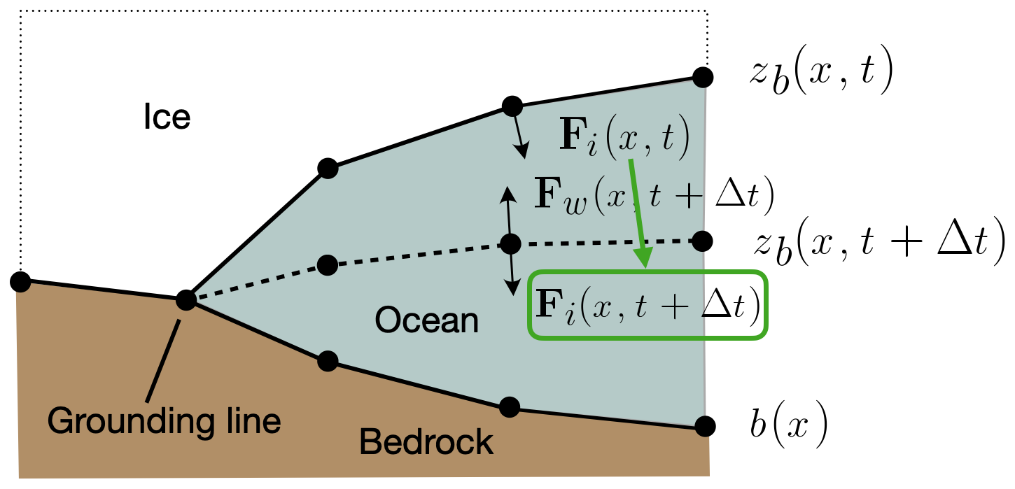
Figure 2 The balance of forces at the ice–ocean boundary. The force due to the ocean pressure, ${\mathit{F}}_{\mathrm{w}}(x,t+\mathrm{\Delta }t)$, is evaluated at the next time step due to the sea spring numerical stabilisation scheme. Prior to this study, the ice load, F_i(x,t), was evaluated at the current time step. By introduction of the FSSA at the ice–ocean interface, the ice load is also evaluated at the next time step. The bed elevation is denoted by b(x), the lower ice surface elevation at the current time step is denoted by z_b(x,t). The predicted lower ice surface elevation at the next time step is denoted by $z_{\mathrm{b}}(x,t+\mathrm{\Delta }t)$.

In order to solve the free-surface equations, they are discretised in time as

$$\begin{array}{}\text{(20)}& z_{\mathrm{s}}^{k+\mathrm{1}}+\mathrm{\Delta }t{u}_x{\displaystyle \frac{\partial z_{\mathrm{s}}^{k+\mathrm{1}}}{\partial x}}+\mathrm{\Delta }t{u}_y{\displaystyle \frac{\partial z_{\mathrm{s}}^{k+\mathrm{1}}}{\partial y}}=z_{\mathrm{s}}^k+\mathrm{\Delta }t(u_z+a_{\mathrm{s}}),\end{array}$$

and

$$\begin{array}{}\text{(21)}& z_{\mathrm{b}}^{k+\mathrm{1}}+\mathrm{\Delta }t{u}_x{\displaystyle \frac{\partial z_{\mathrm{b}}^{k+\mathrm{1}}}{\partial x}}+\mathrm{\Delta }t{u}_y{\displaystyle \frac{\partial z_{\mathrm{b}}^{k+\mathrm{1}}}{\partial y}}=z_{\mathrm{b}}^k+\mathrm{\Delta }t(u_z+a_{\mathrm{b}}).\end{array}$$

In weak form, the equations are multiplied by a test function, ϕ, and integrated over the upper and lower ice surfaces, so that

$$\begin{array}{}\text{(22)}& \begin{array}{rl}{\displaystyle }& {\displaystyle }\underset{{\mathrm{\Gamma }}_{\mathrm{a}}}{\int }\left[z_{\mathrm{s}}^{k+\mathrm{1}}+\mathrm{\Delta }t{u}_x{\displaystyle \frac{\partial z_{\mathrm{s}}}{\partial x}}+\mathrm{\Delta }t{u}_y{\displaystyle \frac{\partial z_{\mathrm{s}}}{\partial y}}\right]\mathit{\varphi }\mathrm{d}\mathrm{\Gamma }\\ {\displaystyle }& {\displaystyle }=\underset{{\mathrm{\Gamma }}_{\mathrm{a}}}{\int }[z_{\mathrm{s}}^k+\mathrm{\Delta }t(u_z+a_{\mathrm{s}}\left)\right]\mathit{\varphi }\mathrm{d}\mathrm{\Gamma }\end{array}\end{array}$$

and

$$\begin{array}{}\text{(23)}& \begin{array}{rl}{\displaystyle }& {\displaystyle }\underset{{\mathrm{\Gamma }}_{\mathrm{a}}}{\int }\left[z_{\mathrm{b}}^{k+\mathrm{1}}+\mathrm{\Delta }t{u}_x{\displaystyle \frac{\partial z_{\mathrm{b}}}{\partial x}}+\mathrm{\Delta }t{u}_y{\displaystyle \frac{\partial z_{\mathrm{b}}}{\partial y}}\right]\mathit{\varphi }\mathrm{d}\mathrm{\Gamma }\\ {\displaystyle }& {\displaystyle }=\underset{{\mathrm{\Gamma }}_{\mathrm{a}}}{\int }[z_{\mathrm{b}}^k+\mathrm{\Delta }t(u_z+a_{\mathrm{b}}\left)\right]\mathit{\varphi }\mathrm{d}\mathrm{\Gamma }.\end{array}\end{array}$$

A backwards difference formula (BDF) time-stepping scheme of first order (i.e., implicit Euler) is employed.

3 Numerical stabilisation of free-surface Stokes problems

The coupling between the Stokes equations and the free-surface dynamics leads to a stiff system, in which the presence of fast-decaying modes (associated with large-magnitude eigenvalues) imposes a severe restriction on the maximum stable time step size, particularly for the explicit time integration methods traditionally used in ice sheet modelling (Löfgren et al., 2022). Physically, this means that a deviation from hydrostatic equilibrium can produce large vertical velocities in the Stokes solution, which, when coupled to the upper and lower free surfaces equations, leads to an overshoot of the upper and lower ice surfaces. In turn, this causes oscillatory behaviour and numerical instability even for very small time steps. To reduce these time step size restrictions, two numerical stabilisation schemes are used here. Firstly, the standard sea spring numerical stabilisation scheme (Durand et al., 2009a) is used, which treats the ocean pressure term implicitly, and the Free-Surface Stabilisation Scheme (FSSA; Kaus et al., 2010) is implemented, which treats the ice load implicitly. The sea spring numerical stabilisation scheme and FSSA complement each other by balancing forces at the ice–ocean interface. Thus far, the FSSA has shown promising results for grounded ice (Löfgren et al., 2022, 2024), but has not previously been implemented for grounding line and floating ice problems. Such model domains are particularly numerically challenging due to sharp gradients in the grounding zone and increased stiffness of the problem. The extension of FSSA to grounding-line problems also opens up the future possibility to construct fully implicit algorithms similar to that of grounded ice in Ahlkrona et al. (2026).

3.1 The sea spring numerical stabilisation scheme

To stabilise the contact problem, a numerical stabilisation scheme called sea spring was implemented on the lower ice surface in (Durand et al., 2009a, Fig. 2). The sea spring numerical stabilisation scheme predicts the lower ice surface, z_b, in the next time step and adjusts the ocean pressure accordingly. The ocean pressure term before numerical stabilisation reads

$$\begin{array}{}\text{(24)}& {\mathit{\sigma }}_{\text{nn}}{|}_{\mathrm{b}}(x,y,t)=-{\mathit{\rho }}_{\mathrm{w}}g(z_{\text{sl}}-z)\end{array}$$

and is evaluated on the current time step, t. Here, z_sl represents the sea level. The lower ice surface elevation at the next time step is predicted using an estimate of the vertical displacement, so that

$$\begin{array}{}\text{(25)}& \begin{array}{rl}{\displaystyle }& {\displaystyle }{z}_{\mathrm{b}}(x,y,t+\mathrm{\Delta }t)\approx z_{\mathrm{b}}(x,y,t)+(\mathit{u}\cdot \widehat{\mathit{n}})\mathrm{\Delta }t\\ {\displaystyle }& {\displaystyle }\times \sqrt{\mathrm{1}+{\left({\displaystyle \frac{\partial z_{\mathrm{b}}(x,y,t)}{\partial x}}\right)}^{\mathrm{2}}+{\left({\displaystyle \frac{\partial z_{\mathrm{b}}(x,y,t)}{\partial y}}\right)}^{\mathrm{2}}},\end{array}\end{array}$$

where Δt is the time step size and t+Δt is the next time step. The ocean pressure term therefore becomes

$$\begin{array}{}\text{(26)}& \begin{array}{rl}{\displaystyle }& {\displaystyle }{\mathit{\sigma }}_{\text{nn}}{|}_{\mathrm{b}}(x,y,t)=-{\mathit{\rho }}_{\mathrm{w}}g\mathit{\{}{z}_{\text{sl}}-z_{\mathrm{b}}(x,y,t)+(\mathit{u}\cdot \widehat{\mathit{n}})\mathrm{\Delta }t\\ {\displaystyle }& {\displaystyle }\times \sqrt{\mathrm{1}+{\left({\displaystyle \frac{\partial z_{\mathrm{b}}(x,y,t)}{\partial x}}\right)}^{\mathrm{2}}+{\left({\displaystyle \frac{\partial z_{\mathrm{b}}(x,y,t)}{\partial y}}\right)}^{\mathrm{2}}}\mathit{\}}\end{array}\end{array}$$

3.2 The Free-Surface Stabilisation Algorithm (FSSA)

The Free-Surface Stabilisation Algorithm (FSSA), was introduced by Kaus et al. (2010) to a Stokes problem with a free surface applied to mantle convection simulations. This method was later extended to Stokes free-surface problems in grounded ice-sheet modelling, proving successful in increasing the largest stable time step size (Löfgren et al., 2022, 2024). Here we will derive the FSSA for floating ice (Fig. 2). The FSSA predicts the free-surface elevation at the next time step, t+Δt, and includes extra terms as boundary conditions to account for the adjustment in ice load. However, contrary to the expression for the ocean pressure, the free surface does not enter explicitly in the formulation for the ice load, but rather through the integral associated with the weak form. The FSSA is derived from Reynold's Transport Theorem,

$$\begin{array}{}\text{(27)}& {\displaystyle \frac{\mathrm{d}}{\mathrm{d}t}}\underset{\mathrm{\Omega }\left(t\right)}{\int }f\mathrm{d}\mathrm{\Omega }=\underset{\mathrm{\Omega }\left(t\right)}{\int }{\displaystyle \frac{\partial f}{\partial t}}\mathrm{d}\mathrm{\Omega }+\underset{\partial \mathrm{\Omega }\left(t\right)}{\int }(\mathit{u}\cdot \widehat{\mathit{n}})f\mathrm{d}\mathrm{\Gamma },\end{array}$$

where f is a physical quantity, Ω(t) is the model domain at time step t and ∂Ω(t) is the domain boundary at time step t. For our purposes, we take $f=-{\mathit{\rho }}_{\mathrm{i}}\mathit{g}\cdot \mathit{v}$, i.e. the right hand side of the Stokes equations multiplied by the test function, v. Reynolds Transport Theorem enables the Stokes equations to account for a spatially evolving domain by incorporating the effect of gravitational forces at the next time step, thereby treating the right hand side implicitly. Assuming that f is time independent, and discretising in time, an approximation is found for the integral of f over the time-discretised domain, at the next time step, Ω^k+1, based on the current time step, k, so that

$$\begin{array}{}\text{(28)}& \underset{{\mathrm{\Omega }}^{k+\mathrm{1}}}{\int }f\mathrm{d}\mathrm{\Omega }\approx \underset{{\mathrm{\Omega }}^k}{\int }f\mathrm{d}\mathrm{\Omega }+\mathrm{\Delta }t\underset{\partial {\mathrm{\Omega }}^k}{\int }(\mathit{u}\cdot \widehat{\mathit{n}})f\mathrm{d}\mathrm{\Gamma }.\end{array}$$

The driving force term, i.e. the right hand side of the Stokes equations, therefore becomes

$$\begin{array}{}\text{(29)}& \begin{array}{rl}{\displaystyle }& {\displaystyle }\underset{{\mathrm{\Omega }}^{k+\mathrm{1}}}{\int }{\mathit{\rho }}_{\mathrm{i}}\mathit{g}\cdot \mathit{v}\mathrm{d}\mathrm{\Omega }\approx \underset{{\mathrm{\Omega }}^k}{\int }{\mathit{\rho }}_{\mathrm{i}}\mathit{g}\cdot \mathit{v}\mathrm{d}\mathrm{\Omega }+\mathrm{\Delta }t\underset{{\mathrm{\Gamma }}_{\mathrm{a}}^k}{\int }(\mathit{u}\cdot \widehat{\mathit{n}}){\mathit{\rho }}_{\mathrm{i}}\mathit{g}\cdot \mathit{v}\mathrm{d}\mathrm{\Gamma }\\ {\displaystyle }& {\displaystyle }+\mathrm{\Delta }t\underset{{\mathrm{\Gamma }}_{\mathrm{o}}^k}{\int }(\mathit{u}\cdot \widehat{\mathit{n}}){\mathit{\rho }}_{\mathrm{i}}\mathit{g}\cdot \mathit{v}\mathrm{d}\mathrm{\Gamma },\end{array}\end{array}$$

where the last two terms represent the predicted upper and lower ice surfaces at the next time step, with an impenetrability condition, $\mathit{u}\cdot \widehat{\mathit{n}}=\mathrm{0}$, at the ice divide and at the ice-bed interface. FSSA is not applied at the calving front because the mesh does not move horizontally here. If an accumulation and melt rate are to be included, two additional terms are added to represent the resulting vertical displacement,

$$\begin{array}{}\text{(30)}& \begin{array}{rl}{\displaystyle }& {\displaystyle }\underset{{\mathrm{\Omega }}^{k+\mathrm{1}}}{\int }{\mathit{\rho }}_{\mathrm{i}}\mathit{g}\cdot \mathit{v}\mathrm{d}\mathrm{\Omega }\approx \underset{{\mathrm{\Omega }}^k}{\int }{\mathit{\rho }}_{\mathrm{i}}\mathit{g}\cdot \mathit{v}\mathrm{d}\mathrm{\Omega }+\mathrm{\Delta }t\underset{{\mathrm{\Gamma }}_{\mathrm{a}}^k}{\int }(\mathit{u}\cdot \widehat{\mathit{n}})({\mathit{\rho }}_{\mathrm{i}}\mathit{g}\cdot \mathit{v})\mathrm{d}\mathrm{\Gamma }\\ {\displaystyle }& {\displaystyle }+\mathrm{\Delta }t\underset{{\mathrm{\Gamma }}_{\mathrm{o}}^k}{\int }(\mathit{u}\cdot \widehat{\mathit{n}})({\mathit{\rho }}_{\mathrm{i}}\mathit{g}\cdot \mathit{v})\mathrm{d}\mathrm{\Gamma }+\mathrm{\Delta }t\underset{{\mathrm{\Gamma }}_{\mathrm{a}}^k}{\int }(a_{\mathrm{s}}{\widehat{\mathit{e}}}_z\cdot \widehat{\mathit{n}})({\mathit{\rho }}_{\mathrm{i}}\mathit{g}\cdot \mathit{v})\mathrm{d}\mathrm{\Gamma }\\ {\displaystyle }& {\displaystyle }+\mathrm{\Delta }t\underset{{\mathrm{\Gamma }}_{\mathrm{o}}^k}{\int }(a_{\mathrm{b}}{\widehat{\mathit{e}}}_z\cdot \widehat{\mathit{n}})({\mathit{\rho }}_{\mathrm{i}}\mathit{g}\cdot \mathit{v})\mathrm{d}\mathrm{\Gamma }\end{array}\end{array}$$

The Stokes equations weak form (Eq. 15) with the FSSA and the sea spring numerical stabilisation scheme therefore become

$$\begin{array}{}\text{(31)}& \begin{array}{rl}{\displaystyle }& {\displaystyle }-\underset{{\mathrm{\Omega }}^k}{\int }\mathit{\tau }:\mathrm{\nabla }\mathit{v}\mathrm{d}\mathrm{\Omega }-\underset{{\mathrm{\Gamma }}_{\mathrm{o}}^k\cup {\mathrm{\Gamma }}_{\mathrm{c}}^k}{\int }{\mathit{\rho }}_{\mathrm{w}}g\mathrm{\Delta }t({\stackrel{\mathrm{̃}}{\mathit{u}}}^{k+\mathrm{1}}\cdot \widehat{\mathit{n}})\\ {\displaystyle }& {\displaystyle }\times \sqrt{\mathrm{1}+{\left({\displaystyle \frac{\partial z_{\mathrm{b}}}{\partial x}}\right)}^{\mathrm{2}}+{\left({\displaystyle \frac{\partial z_{\mathrm{b}}}{\partial y}}\right)}^{\mathrm{2}}}\widehat{\mathit{n}}\cdot \mathit{v}\mathrm{d}\mathrm{\Gamma }\\ {\displaystyle }& {\displaystyle }-\underset{{\mathrm{\Gamma }}_{\mathrm{b}}^k}{\int }C|{\stackrel{\mathrm{̃}}{\mathit{u}}}_{\mathrm{b}}^{k+\mathrm{1}}{|}^{m-\mathrm{1}}{\stackrel{\mathrm{̃}}{\mathit{u}}}_{\mathrm{b}}^{k+\mathrm{1}}\cdot \mathit{v}\mathrm{d}\mathrm{\Gamma }+\underset{{\mathrm{\Omega }}^k}{\int }p\mathrm{\nabla }\cdot \mathit{v}\mathrm{d}\mathrm{\Omega }\\ {\displaystyle }& {\displaystyle }-\mathit{\theta }\mathrm{\Delta }t\underset{{\mathrm{\Gamma }}_{\mathrm{a}}^k}{\int }({\stackrel{\mathrm{̃}}{\mathit{u}}}^{k+\mathrm{1}}\cdot \widehat{\mathit{n}})({\mathit{\rho }}_{\mathrm{i}}\mathit{g}\cdot \mathit{v})\mathrm{d}\mathrm{\Gamma }\\ {\displaystyle }& {\displaystyle }-\mathit{\theta }\mathrm{\Delta }t\underset{{\mathrm{\Gamma }}_{\mathrm{o}}^k}{\int }({\stackrel{\mathrm{̃}}{\mathit{u}}}^{k+\mathrm{1}}\cdot \widehat{\mathit{n}})({\mathit{\rho }}_{\mathrm{i}}\mathit{g}\cdot \mathit{v})\mathrm{d}\mathrm{\Gamma }\\ {\displaystyle }& {\displaystyle }=\underset{{\mathrm{\Omega }}^k}{\int }{\mathit{\rho }}_{\mathrm{i}}\mathit{g}\cdot \mathit{v}\mathrm{d}\mathrm{\Omega }-\underset{{\mathrm{\Gamma }}_{\mathrm{o}}^k\cup {\mathrm{\Gamma }}_{\mathrm{c}}^k}{\int }{\mathit{\rho }}_{\mathrm{w}}gz\widehat{\mathit{n}}\cdot \mathit{v}\mathrm{d}\mathrm{\Gamma }\\ {\displaystyle }& {\displaystyle }+\mathit{\theta }\mathrm{\Delta }t\underset{{\mathrm{\Gamma }}_{\mathrm{a}}^k}{\int }(a_{\mathrm{s}}{\widehat{\mathit{e}}}_z\cdot \widehat{\mathit{n}})({\mathit{\rho }}_{\mathrm{i}}\mathit{g}\cdot \mathit{v})\mathrm{d}\mathrm{\Gamma }\\ {\displaystyle }& {\displaystyle }+\mathit{\theta }\mathrm{\Delta }t\underset{{\mathrm{\Gamma }}_{\mathrm{o}}^k}{\int }(a_{\mathrm{b}}{\widehat{\mathit{e}}}_z\cdot \widehat{\mathit{n}})({\mathit{\rho }}_{\mathrm{i}}\mathit{g}\cdot \mathit{v})\mathrm{d}\mathrm{\Gamma }\end{array}\end{array}$$

where we have assumed the sea level to be z_sl=0 and the ocean pressure was applied only on the portion of the calving front in contact with the ocean, ${\mathrm{\Gamma }}_{\mathrm{c}}^k$. Here, ${\stackrel{\mathrm{̃}}{\mathit{u}}}^{k+\mathrm{1}}$ is an approximation of the velocity at the next time step, k+1. Since the calving front, Γ_o, does not move horizontally, the FSSA terms are identical to zero there. Here, the parameter θ has been introduced to allow adjustment of the FSSA terms. A value of θ=0 disables the FSSA terms, while a value of θ=1 fully activates the FSSA terms. Finally, the weak form of the incompressibility condition reads

$$\begin{array}{}\text{(32)}& -\underset{{\mathrm{\Omega }}^k}{\int }\mathrm{\nabla }\cdot {\stackrel{\mathrm{̃}}{\mathit{u}}}^{k+\mathrm{1}}q\mathrm{d}\mathrm{\Omega }=\mathrm{0}.\end{array}$$

Note that whether the FSSA and sea spring are active or not at the lower and upper ice surfaces has an effect on the force balance at those surfaces due to the opposing ice load and ocean pressure. When both the sea spring numerical stabilisation scheme and FSSA are active, both the ocean pressure and the ice load are evaluated at the next time step, which results in a balance of forces. When only the sea spring numerical stabilisation is activated, the ocean pressure is evaluated at the predicted surface at the next time step. As a result, the ocean pressure contribution in the Stokes equations is higher in an advancing case, i.e. when the ice is thickening, compared to evaluating the ocean pressure at the current ice surface. The opposite is true in the retreating case, i.e. the ocean pressure contribution is lower with sea spring because it predicts thinner ice. In contrast, including the FSSA term at the lower ice surface predicts a higher ice load in an advancing case due to the prediction of thicker ice and a lower ice load in a retreating case due to the prediction of thinner ice.

3.3 Numerical implementation of grounding-line migration

During a transient simulation, the grounding line position must be allowed to migrate to reflect the altering ice geometry and velocity. Once a new grounding line position is determined, the application of boundary conditions must be altered accordingly. To determine whether to apply a friction law and an impenetrability condition or whether to apply ocean pressure and a free-slip condition at a particular node, the normal stress and the ocean pressure are examined through an algorithm presented in (Durand et al., 2009a).

During discretization and global assembly of the Stokes equations, the left hand side is split into the mass matrix, K, and the solution vector, U and the right hand side is the force vector, F. Once solved, the residual can be obtained,

$$\begin{array}{}\text{(33)}& \mathbf{R}=\mathbf{K}\mathit{U}-\mathit{F}.\end{array}$$

When an exact solution is obtained, only the components in R corresponding to nodes where a Dirichlet boundary condition is applied are non zero and are equal to the ice load force, or equivalently the normal stress, at that node. This nodal force is used to evaluate whether the ice-bed boundary conditions should be applied, i.e. if $z_{\mathrm{b}}(x,y,t)=b(x,y)$ and $-{\mathit{\sigma }}_{\text{nn}}{|}_{\mathrm{b}}>p_{\mathrm{w}}(z_{\mathrm{b}},t)$, or whether ice–ocean boundary conditions should be applied, i.e. $z_{\mathrm{b}}(x,y,t)>b\left(x\right)$ or $z_{\mathrm{b}}(x,y,t)=b\left(x\right)$ and $-{\mathit{\sigma }}_{\text{nn}}{|}_{\mathrm{b}}\le p_{\mathrm{w}}(z_{\mathrm{b}},y)$.

When solving the Stokes equations, the boundary conditions are first determined a priori by checking only whether $z_{\mathrm{b}}(x,y,t)=b(x,y)$ and applying ice-bed boundary conditions or otherwise applying ice–ocean boundary conditions. Once the Stokes equations are solved to a convergence tolerance of 10⁻³, the balance of forces is re-evaluated and the boundary conditions are altered once in the nonlinear Stokes iterations per time step.

Algorithm 1 Marine ice-sheet simulation.

1:

Initialise mesh Ω⁰

2:

for each time-step k do

3:

r=0; s=0

4:

while $\Vert {\mathit{U}}_{r+\mathrm{1}}^{k+\mathrm{1}}-{\mathit{U}}_r^{k+\mathrm{1}}\Vert >{\mathrm{10}}^{-\mathrm{3}}$ and $r<r_{max}$ do

5:

Solve Stokes eq. for $({\mathit{u}}_{\mathrm{r}}^{k+\mathrm{1}},p_{\mathrm{r}}^{k+\mathrm{1}})$

6:

$r:=r+\mathrm{1}$

7:

end while

8:

Adjust boundary conditions based on residual

9:

while $\Vert {\mathit{U}}_{r+\mathrm{1}}^{k+\mathrm{1}}-{\mathit{U}}_r^{k+\mathrm{1}}\Vert >{\mathrm{10}}^{-\mathrm{5}}$ and $r<r_{max}$ do

10:

Solve Stokes eq. for $({\mathit{u}}_{\mathrm{r}}^{k+\mathrm{1}},p_{\mathrm{r}}^{k+\mathrm{1}})$

11:

$r:=r+\mathrm{1}$

12:

end while

13:

for z in {z_s,z_b} do

14:

Mark nodes z_j active if $b(x,y)\le z_{\mathrm{b}}(x,y,t)<z_{\mathrm{s}}(x,y,t)$ false

15:

while $\Vert {\mathit{z}}_{\mathrm{s}+\mathrm{1}}^{k+\mathrm{1}}-{\mathit{z}}_{\mathrm{s}}^{k+\mathrm{1}}\Vert >{\mathrm{10}}^{-\mathrm{5}}$ and s<s_max do

16:

If s≠0, adjust (in)active nodes based on previous residual

17:

Set M_ij=δ_ij for active nodes z_j

18:

Set f_i to corresponding lower/upper limit

19:

Solve the free-surface eq. for ${\mathit{z}}_{\mathrm{s}}^{k+\mathrm{1}}$

20:

$s:=s+\mathrm{1}$

21:

end while

22:

end for

23:

Update mesh Ω^k+1

24:

$z_{\mathrm{s}}^k:=z_{\mathrm{s}}^{k+\mathrm{1}}$; $z_{\mathrm{b}}^k:=z_{\mathrm{b}}^{k+\mathrm{1}}$; $({\mathit{u}}^k,p^k):=({\mathit{u}}^{k+\mathrm{1}},p^{k+\mathrm{1}})$

25:

end for

Once the Stokes solver has converged, the resulting velocities are used to calculate the free-surface evolution. Here, we describe the evolution of the lower ice surface. Again, a system of equations in weak form must be solved,

$$\begin{array}{}\text{(34)}& \mathbf{M}{{\mathit{z}}_{\mathbf{b}}}^{k+\mathrm{1}}=\mathit{f},\end{array}$$

where z_b is the solution vector for the ice surface elevation at the next time step, M is the matrix of coefficients and f is the vector representing all terms in Eq. (23) that do not contain the variable $z_{\mathrm{b}}^{k+\mathrm{1}}$. While solving the free-surface evolution equation, a node $z_{\mathrm{b},j}=z_{\mathrm{b}}(x,y,t)$ is marked as active if it does not satisfy the condition $b(x,y)\le z_{\mathrm{b}}(x,y,t)<z_{\mathrm{s}}(x,y,t)$.

For each node z_b,j marked as active, the system matrix is altered so that M_ij=δ_ij, where δ_ij is the Kronecker delta defined by δ_ij=1 if i=j and δ_ij=0 if i≠j. If the node is marked as active because $z_{\mathrm{b},j}<b_j$, the corresponding component of f is set to f_i=b_j. Alternatively, if $z_{\mathrm{b},j}\ge z_{\mathrm{s},j}$, the corresponding right-hand side component is set to $f_i=z_{\mathrm{s},j}$.

The system is solved repeatedly until the convergence tolerance is reached. Between each solve, the residual is solved,

$$\begin{array}{}\text{(35)}& \mathit{r}=\mathbf{M}{\mathit{z}}_{\mathbf{b}}-\mathit{f}.\end{array}$$

This is used to determine the set of active and inactive nodes in the next solve.

If a node was previously active because $z_{\mathrm{b},j}<b_j$ has a residual r_j<0, then it is marked inactive. On the other hand, if a node was previously active because $z_{\mathrm{b},j}\ge z_{\mathrm{s},j}$, then a residual of r_j>0 results in the node being marked inactive. Similarly, a node can become active if it satisfies $b(x,y)\le z_{\mathrm{b}}(x,y,t)<z_s(x,y,t)$.

4 Idealised numerical experiments – the MISMIP experiment

In order to investigate the speedup and accuracy of the FSSA across various spatial and temporal resolutions in simulations of marine ice sheets, we choose to perform experiments with the Marine Ice Sheet Model Intercomparison Project (MISMIP, Pattyn et al., 2012, Fig. 3) framework. The MISMIP experiments test the ability of models to capture the marine ice-sheet instability (MISI), whereby the position of the grounding line is stable on prograde slopes and unstable on retrograde slopes (Schoof, 2007; Durand et al., 2009a). The ability of models to capture MISI is paramount for accurately simulating past and future grounding-line migration and the associated sea-level contribution of glaciers such as Thwaites and Pine Island, which are particularly susceptible (Bett et al., 2024).

The focus of this part of the study is on the MISMIP Experiment 3a (Durand et al., 2009a; Pattyn et al., 2012). We use this setup to investigate the size of the largest stable time-step as well as the accuracy when using FSSA. We also study the effect of the improved force balance in floating ice when including both the FSSA and the sea spring numerical stabilisation schemes and compare simulation runtimes.

4.1 Numerical experiments

Simulations with FSSA activated (θ=1) are performed with time-step sizes of $\mathrm{\Delta }t=\mathrm{0.5},\mathrm{10}$ and 50 years and varying grounding zone resolution (Table 3). A reference simulation of the full advance and retreat phases without the FSSA terms (θ=0) is performed for a time step size of Δt=0.5 and a grounding-zone horizontal resolution of 200 m (Table 3). A finer spatial resolution is computationally infeasible because a time step size of Δt=0.5 is too small to allow for reasonable simulation times. All simulations are subject to a small time step of 0.5 years for 1000 years after the ice fluidity jump in the retreating phase of Exp. 3a. When a small time step size is not used for a short period of time during the ice fluidity jump, the upper and lower surfaces, as well as the velocity field, exhibited oscillatory behaviour, leading to numerical stability.

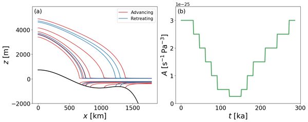
The MISMIP Exp. 3a is defined by a 2D modelling domain of a marine ice sheet with the x-axis denoting the horizontal direction and the z-axis denoting the vertical direction. We apply the Stokes model and assume invariance in the y-direction. The bed elevation for Exp. 3a is defined as

$$\begin{array}{}\text{(36)}& \begin{array}{rl}{\displaystyle }b\left(x\right)=& {\displaystyle }\mathrm{729}-\mathrm{2184.8}{\left({\displaystyle \frac{x}{\mathrm{750}\mathrm{000}}}\right)}^{\mathrm{2}}+\mathrm{1031.72}{\left({\displaystyle \frac{x}{\mathrm{750}\mathrm{000}}}\right)}^{\mathrm{4}}\\ {\displaystyle }& {\displaystyle }-\mathrm{151.72}{\left({\displaystyle \frac{x}{\mathrm{750}\mathrm{000}}}\right)}^{\mathrm{6}}.\end{array}\end{array}$$

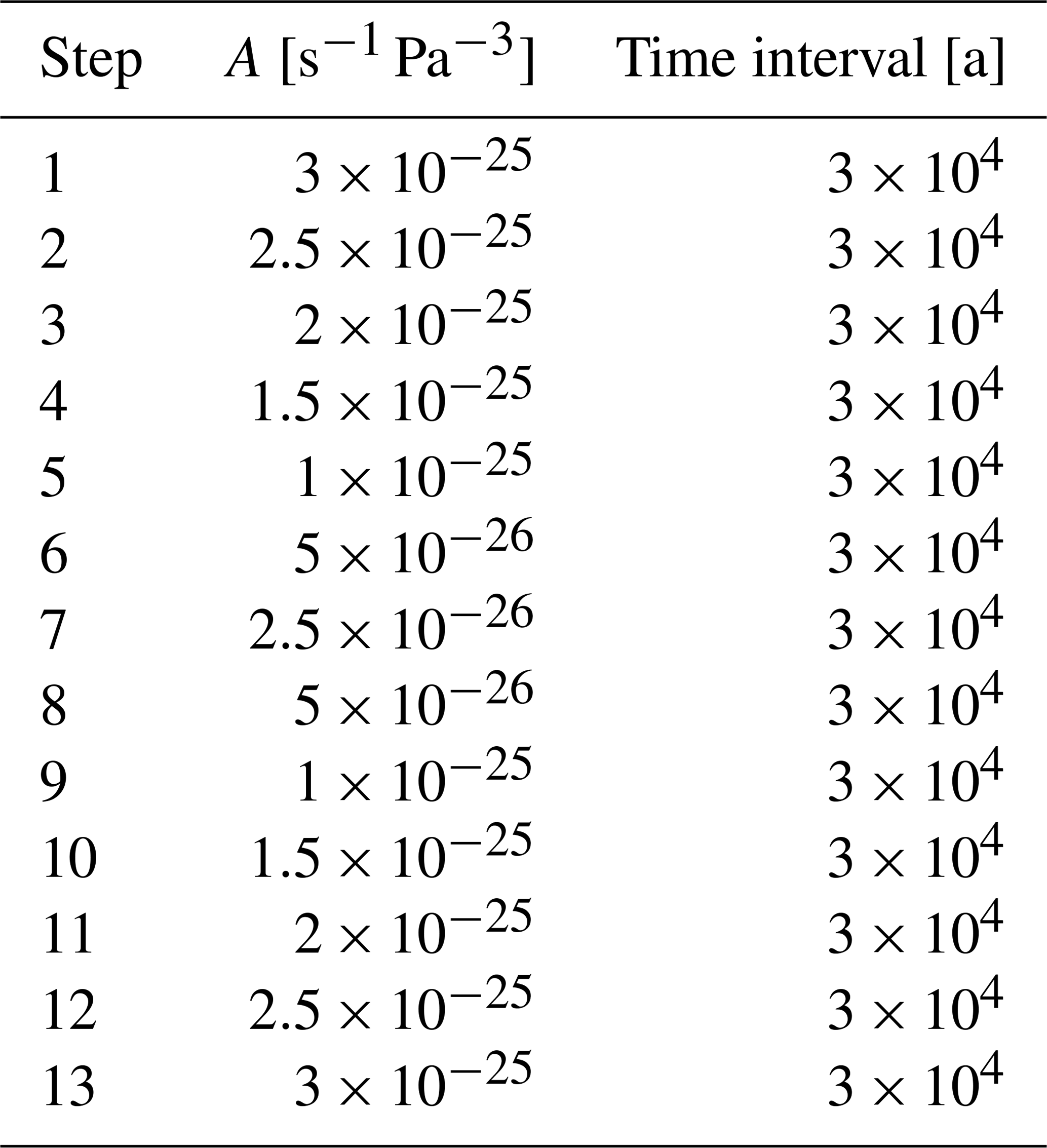
The model domain is initialised with a 10 m thick ice sheet and ice shelf. Initially, the floating ice is prescribed to be in hydrostatic equilibrium, a constraint which is only enforced to construct the initial geometry. The model parameters remain fixed throughout the simulations, with the exception of the ice fluidity A, and are defined in Table 1. The ice fluidity, A, is altered at 12 time points during the simulation, according to the values provided in Table 2. The step-wise change in fluidity induces grounding-line advance as the ice becomes stiffer (decreasing A) and grounding-line retreat as the ice becomes softer (increasing A). The experiment is carried out over a period of 285 000 years and demonstrates the typical hysteretic behaviour of the grounding line in areas of alternating pro- and retrograde slopes. As outlined in the MISMIP study (Pattyn et al., 2012), the first 10 000 years of Exp. 3a are prone to numerical instability due to the thin, unrealistic nature of the domain. We chose a numerically-stable set up, which allowed quick simulation of these first 10 000 years. The chosen setup was performed with a time step size of Δt=10 years and a horizontal resolution of Δx=2000 m throughout the domain. Each simulation in our experiment, as outlined in Table 3, is performed beginning with the geometry at t=10 000 years.

Table 1 The model parameters implemented in Elmer/Ice for the 2D MISMIP Exp. 3a (Pattyn et al., 2012), used to investigate the application of the FSSA to the ice–ocean interface. The temporally-varying ice fluidity, A, is defined below in Table 2.

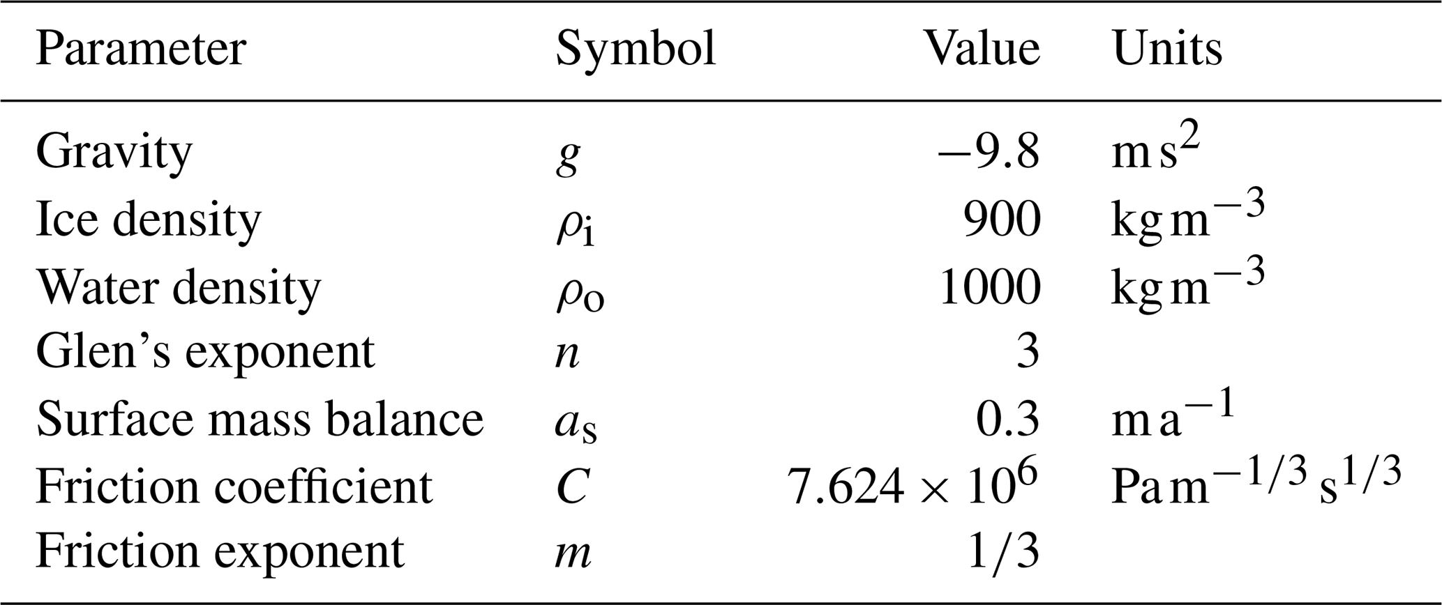
Table 2 The ice fluidity, A, for the time intervals outlined in the MISMIP Exp. 3a (Pattyn et al., 2012). Note that the ice fluidity decreases in steps 1–7 and increases in steps 7–13.

Meshes are constructed from a 1D footprint mesh, which is vertically extruded to 20 layers, forming a terrain-following mesh consisting of quadrilateral elements. The footprint is refined in the areas either side of the grounding line position, in a 100 km wide area that we refer to as the grounding zone hereafter. The grounding zone resolutions tested are $\mathrm{\Delta }x=\mathrm{25},\mathrm{50},\mathrm{100}$ and 200 m (Table 3). Outside the refined area, a gradually decreasing horizontal resolution is applied to avoid large jumps in element size from the refined to the more coarsely resolved area, i.e. to ensure good mesh quality. Every 500 years, the mesh is updated, ensuring that the grounding line always remains within the area of refined horizontal resolution. This is done by finding the grounding line position, x_GL, and defining the region within which the horizontal mesh should be refined, i.e. $[x_{\text{GL}}-\mathrm{50},x_{\text{GL}}+\mathrm{50}]\mathrm{km}$. Outside this region, a linearly decreasing resolution is prescribed. The number of nodes in the area with a coarser horizontal resolution is defined in such a way that the number remains the same throughout the simulations. Further implementation details using the Gmsh software (Geuzaine and Remacle, 2009) can be found in Henry (2026). The simulations with a refined horizontal resolution of Δx=25 m contain 98 679 nodes, those with Δx=50 m contain 56 679 nodes, those with Δx=100 m contain 35 679 nodes and those with Δx=200 m contain 25 179 nodes. Each node has 3 degrees of freedom, corresponding to the horizontal velocities, (u_x,u_z), and pressure, p.

Table 3 The choice of parameters for the simulations using the MISMIP Exp. 3a modelling framework. Only parameter choices yielding stable results are listed. The parameters are the time step size, Δt, the horizontal grounding-zone resolution, Δx, and the parameter controlling the activation of the FSSA, θ. This parameter takes the value θ=1 when the FSSA is active and θ=1 when the FSSA is inactive. Note that the largest stable time step is between 0.5 and 2 years.

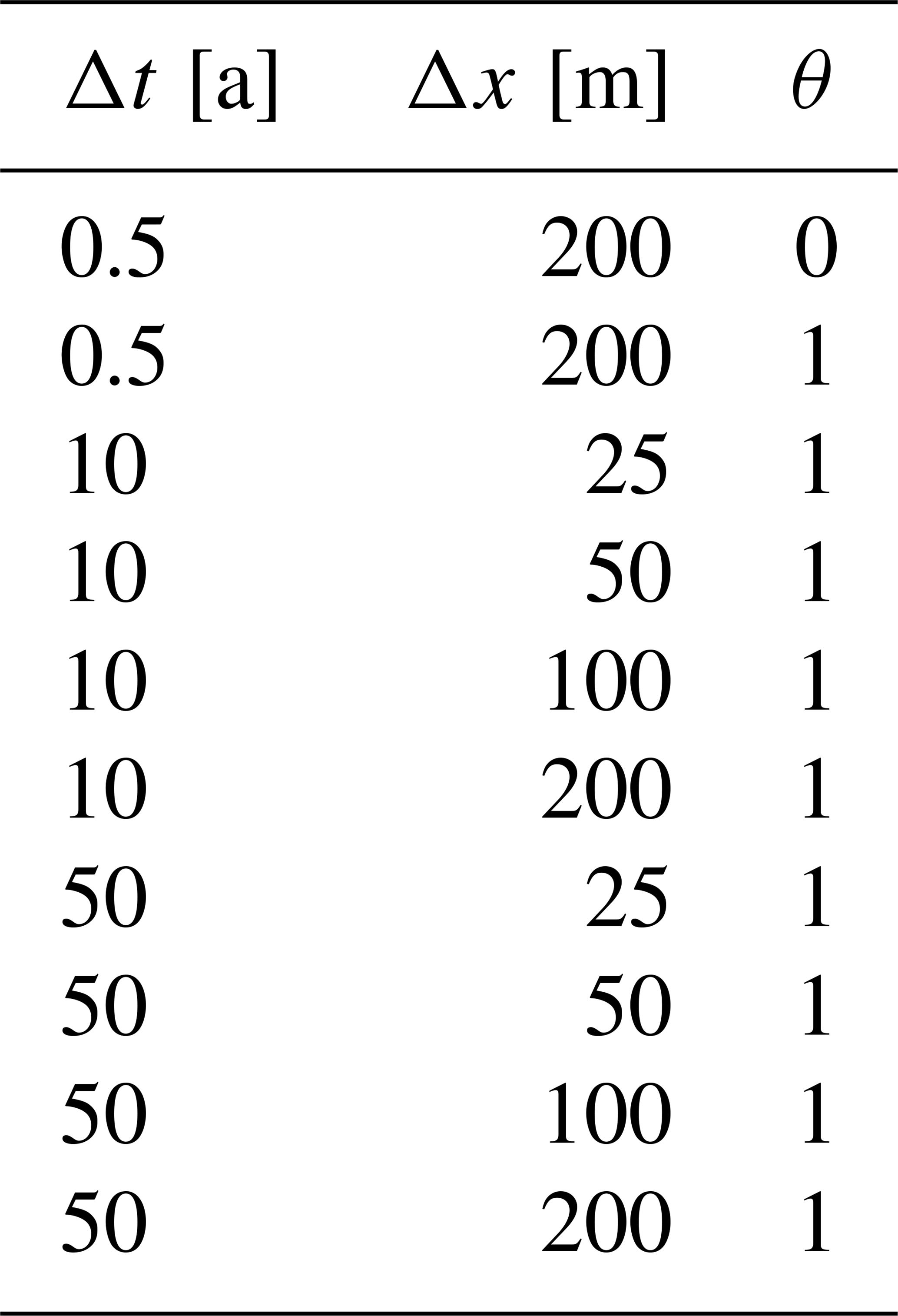
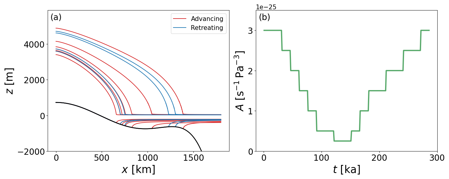
Figure 3 The MISMIP Exp. 3a (Pattyn et al., 2012) is designed to demonstrate grounding line migration over prograde and retrograde slopes, see the solid black line showing the bed elevation in (a). The movement of the grounding line is induced by altering the ice fluidity, A, at certain intervals during transient simulation as seen in (b). As the ice fluidity is reduced, the grounding line advances (red lines, (a)) and as the ice fluidity is increased, the grounding line retreats (blue lines, (a)).

Linear finite elements for velocity and pressure are used, with the Bubbles stabilisation (Baiocchi et al., 1993). The choice of linear elements is justified by the convergence tests in Gagliardini et al. (2013), which showed no improvement in accuracy when using quadratic elements for velocity and linear elements for pressure. The Stokes equations are solved using the Multifrontal Massively Parallel sparse direct Solver (MUMPS, Amestoy et al., 2001). In each time-step, first the Stokes equations are solved, followed by the upper free-surface and finally the lower free-surface equation.

Picard fixed point iterations are used to resolve the non-linear viscosity, with a nonlinear system convergence tolerance of 10⁻⁵ using a relaxation factor of 0.9. The free surface Eqs. (16) and (17) are solved semi-implicitly, using a velocity from the last Stokes iteration (i.e explicit treatment) but an implicit treatment of the surface itself. The linear convergence tolerance is set to 10⁻⁶ for both the upper and lower ice surfaces using the biconjugate gradient stabilised (BiCGStab) method, preconditioned using incomplete LU factorisation (ILU0). The minimum ice thickness is set to 10 m and is activated when solving the free-surface evolution equation for the upper ice surface. Due to the variational inequality, which sets the upper and lower limits of the free surfaces, nonlinear iterations with a convergence tolerance is set to 10⁻⁵ are performed to solve the free surface evolution equation. The streamline upwind/Petrov-Galerkin (SUPG) method is used for numerical stabilisation of the free surface solvers (Franca and Frey, 1992). The MISMIP simulations were performed in serial on the Dardel high-performance computing system (PDC Center for High Performance Computing), using the CPU partition with AMD EPYC Zen2 processors.

4.2 Results

The grounding line first advances and then retreats. Directly after each jump in ice fluidity, A, the grounding line advanced or retreated more rapidly for a period of time before slowing down. The slope of the bed also had an influence on how rapidly the grounding line advanced or retreated. During advance, the grounding line was first on a prograde slope. Once it had advanced enough to reach the area with a retrograde slope, it advanced more rapidly. In the retreating phase, the grounding line retreated more rapidly when on the retrograde slope and more slowly on the prograde slope.

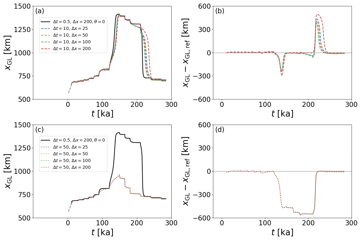
Figure 4 The grounding line position, x_GL, is plotted against the simulation time, t, in (a, c). The difference between the grounding line position, x_GL, of each simulation compared with the reference grounding line position, x_GL,ref, is plotted in (b, d). The black solid lines indicate a time step size of Δt=0.5 years, the dashed lines in (a, b) indicate a time step size of Δt=10 years and the dotted lines in (c, d) indicate a time step size of Δt=50 years. The line colours indicate the horizontal resolution in the refined area encompassing the grounding line. Blue indicates a resolution of Δx=25 m, orange a resolution of Δx=50 m, green a resolution of Δx=100 m, and red a resolution of Δx=200 m. Please note that differences in grounding line position between simulations with a time step of Δt=50 are negligible.

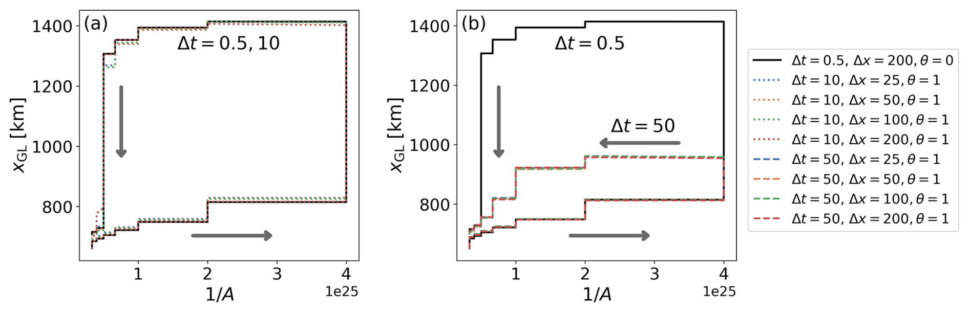
Figure 5 The hysteretic behaviour of the grounding line on alternating retro- and prograde slopes according to the MISMIP Exp. 3a, with time step sizes of Δt=10 years in (a) and Δt=50 years in (b). The simulations with larger time step sizes are compared to a simulation with a time step size of Δt=0.5. The grounding line position, x_GL is plotted as a function of the inverse ice fluidity, $\mathrm{1}/A$, across various time step sizes and grounding-zone horizontal resolutions. All simulations are stabilised with the FSSA (θ=1) except for the simulation with a set up of Δt=0.5, $\mathrm{\Delta }x=\mathrm{200},\mathit{\theta }=\mathrm{0}$ (black line).

Even for small time-step sizes, much lower than those presented here, no simulation was possible without sea spring. Simulations without the FSSA (θ=0) were not numerically stable with time step sizes of 10 and 50 years. The FSSA-stabilised simulations with a time-step size of Δt=10 and Δt=50 years were numerically stable. The simulations with Δt=10 also showed high accuracy (Fig. 4). With this time-step size, the maximum grounding line extent ranged from 1413 km in the case of the simulation with a horizontal grounding-zone resolution of Δx=25 m to 1406 km in the case of the simulation with a horizontal grounding-zone resolution of Δx=200 m, both close to the maximum grounding line extent of 1414 km in the reference simulation with Δt=0.5, Δx=200 and θ=0.

The simulations with Δt=10 lagged behind the reference simulations during rapid grounding line advance, i.e. when the grounding line position was on the retrograde slope and the grounding line position was unstable. The maximum lag of the grounding line position ranged from of 244 km in the case of the simulation with $\mathrm{\Delta }x=\mathrm{25}-\mathrm{297}\mathrm{m}$ with a horizontal grounding-zone resolution of Δx=200 m. During rapid grounding line retreat, when the grounding line position was unstable, the simulations lagged further behind the reference simulation, with the Δx=25 simulation lagging a maximum of 431 km and the Δx=200 simulation lagging a maximum of 494 km behind the reference simulation. There is no clear relation between spatial resolution and the lag. This lag occurs despite the precaution of applying a small time step size of 0.5 years immediately after each ice fluidity jump.

In the simulations with a time-step size of Δt=50 years, the grounding line did not follow the full hysteretic behaviour expected of this experiment (Fig. 5), although approximately the same steady state was eventually reached, and the simulation was very accurate in phases of slow migration. The grounding line reached maximum extents ranging between 958 and 962 km (depending on the resolution $\mathrm{\Delta }x=\mathrm{25},\mathrm{50},\mathrm{100}$, and 200 m) compared with a maximum extent of 1414 km in the reference simulation.

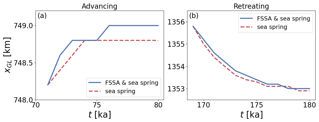
Figure 6 Grounding line migration in (a) during advance of the grounding line, and (b) during retreat of the grounding line. The blue curves indicate simulations which include both the sea spring numerical stabilisation scheme and the FSSA(θ=1), while the dashed red curves indicate simulations with only the sea spring numerical stabilisation scheme (θ=0). These simulations have been performed with a refined mesh of 200 m in the area surrounding the grounding line and a time step size of 0.5 years.

In Fig. 4 there is no significant difference between simulations with and without FSSA for a small time-step size of Δt=0.5 when analysed on the timescale of the entire MISMIP experiment. However, during periods of rapid advance and retreat, a small difference is observed due to evaluating the ice load and the ocean pressure at the same time step (θ=1) compared to at different time steps (θ=0), see Fig. 6. There is a small influence on the grounding line position, with FSSA simulations having a grounding line further oceanward throughout the simulation time, with the simulation that includes the FSSA being on average 1030 m further oceanward in the advancing phase and 635 m further oceanward in the retreating phase. In other words, the grounding line advances more quickly and retreats more slowly in the simulation with the FSSA active (θ=1) compared to the simulation without the FSSA terms (θ=0). The reasons for this mismatch are discussed in Sect. 6.1.

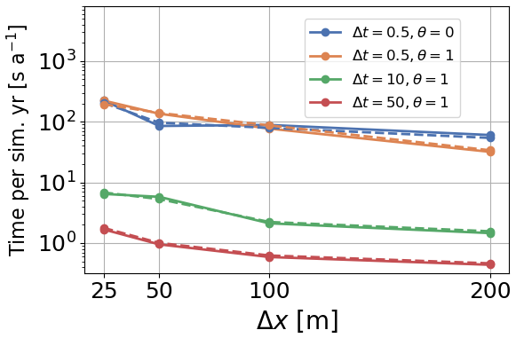
Figure 7 The average CPU time (solid lines) and the wall time (dashed lines) per simulation year for MISMIP Exp. 3a over 500 simulation years starting at t=10 000 year. The colours indicate the time step size, Δt, and whether the FSSA is active (θ=1) or inactive (θ=0). Results are shown for refined horizontal mesh resolutions of 25, 50, 100, and 200 m.

Incorporating FSSA resulted in a significant improvement in computational efficiency compared to simulations without it (Fig. 7). Without the FSSA, a time step size of Δt=5 did not converge after a short time and a time step size of Δt=2 converged well in the advancing phase but did not converge in the retreating phase even with the standard short periods of a smaller time step immediately after the viscosity jumps. In contrast, a time step size as large as 250 years is numerically stable using FSSA, albeit with error. The time step size of Δt=50 resulted in a speedup range of 38–43 compared to a time-step of 2, when measured from t=10 000 for 500 years and the time step size of Δt=10 resulted in a speedup of 11. In simulations with a horizontal grounding-zone resolution of Δx=25 m, the speedup between time step sizes of Δt=10 and Δt=50 was 4.4. Simulations with a horizontal grounding-zone resolutions of Δx=200 m showed a similar speed up of 3.8 when comparing time step sizes of Δt=10 and Δt=50.

5 Application to Ekström Ice Shelf

5.1 Numerical experiments

In order to evaluate our FSSA modelling framework in the context of a 3D, real-world, grounding-line problem, we apply the FSSA-stabilised model to the Ekström Ice Shelf embayment in Dronning Maud Land, East Antarctica (Fig. 8). Ekström Ice Shelf has a length of ∼120 km compared to a width of only ∼50 km and is strongly influenced by lateral buttressing caused by the Søråsen and Halvfarryggen Ice Rises, resulting in a relatively thick ice shelf. Ekström Ice Shelf has been the subject of numerous studies, including comprehensive mapping of the ice shelf cavity and related studies (e.g. Neckel et al., 2012; Schannwell et al., 2019; Smith et al., 2020; Eisermann et al., 2020; Oetting et al., 2022). Moving to a 3D, real-world setting allows validation of the FSSA across a variety of flow regimes and grounding line behaviours.

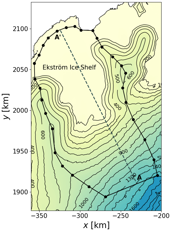
Figure 8 The upper ice surface elevation, z_s, relative to the mean sea level of Ekström Ice Shelf Embayment in Dronning Maud Land, East Antarctica. The solid line shows the model domain for the 3D full Stokes simulations of the embayment. The grey dashed line shows the location of a cross-section, $\mathbf{A}-{\mathbf{A}}^{\prime }$, made through the 3D simulation. The open ocean can be seen in white in the upper left corner.

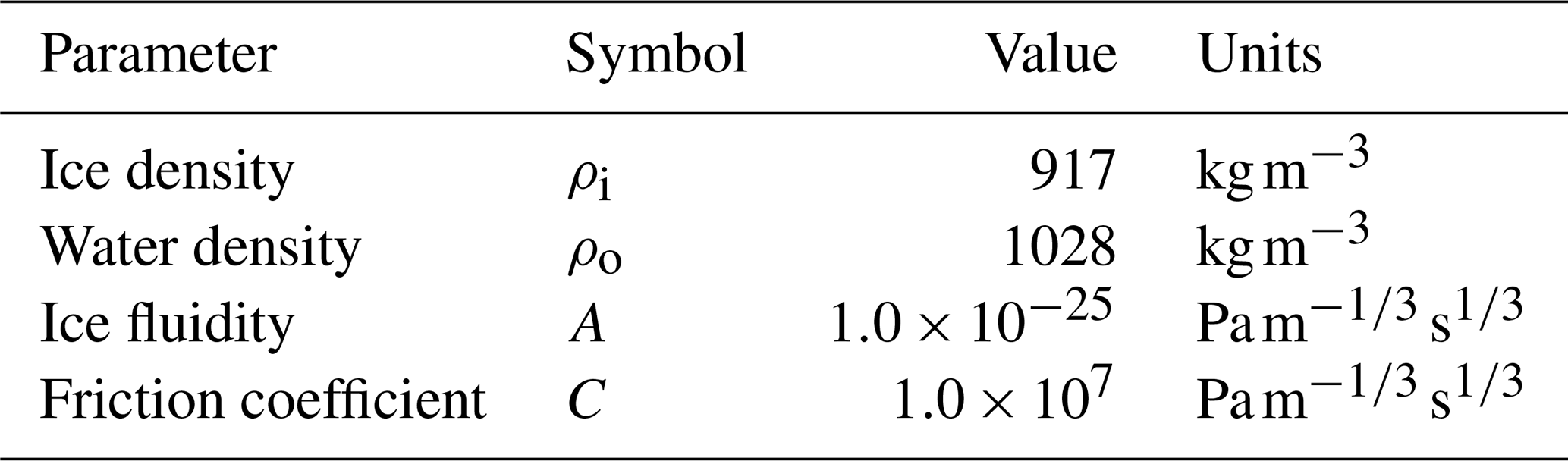
In order to model Ekström Ice Shelf, a number of changes were made in comparison to the idealised experiments above. Several parameters are given more accurate values (e.g. Morlighem et al., 2020), as laid out in Table 4. The spatially constant isothermal ice fluidity, A, and the friction coefficient, C, were tuned to values that caused minimal deviation from observed surface velocities (Rignot et al., 2017) in an ad hoc manner given that the purpose of the study is to investigate the applicability of FSSA and not to make projections. The geometry of the initial upper ice surface, the lower ice surface and the bed elevation were derived from Morlighem et al. (2020). For the surface accumulation rate, a_s, we used the results of the Regional Atmospheric Climate Model (RACMO2.3p1, van den Broeke, 2019). The basal melt rates are derived from Adusumilli et al. (2020) and a condition is applied to ensure that the melt occurs only at floating nodes. The surface accumulation rate and the basal melt rate are included in the free-surface evolution equations (Eqs. 16 and 17), and the FSSA accumulation terms, i.e. the last two terms of Eq. (31). No smoothing of the initial upper and lower ice surface, the bed elevation nor the surface accumulation rate was made. However, significant fluctuations in the basal mass balance caused excess thinning of the ice in isolated areas and numerical instabilities regardless of whether the FSSA was active or not. Therefore, $\text{anomalies}>\mathrm{4}\mathrm{m}{\mathrm{a}}^{-\mathrm{1}}$ were removed and smoothing of the basal melt rate dataset was performed with a Gaussian filter.

Table 4 The model parameters for the 3D Ekström ice shelf experiments to test the time step size and accuracy of transient simulations when applying the FSSA to the ice–ocean interface. All other model parameters are as in Table 1.

The horizontal boundaries of the model domain were chosen along divides and streamlines, and close to the calving front. In the interior portion of the embayment, the low ice thickness (<10 m in some areas) and the roughness of the bed caused numerical instability. We therefore chose to reduce the inland extent of the domain slightly to avoid these numerical instabilities, which is justified because the velocities are low in this area and have only a negligible influence on the overall ice-flow dynamics of the downstream embayment.

The 3D finite element mesh is constructed using an unstructured mesh footprint with a horizontal resolution of Δx=500 m in an area 3000 m either side of the grounding line and a horizontal resolution of Δx=2000 m elsewhere. The horizontal mesh footprint is vertically extruded for a total of 6 layers, allowing for high horizontal resolution at the grounding line and a reasonable compute time. The mesh contains 18 343 nodes, meaning that there are 73 372 degrees of freedom and the simulations are performed with 100 partitions using CPU partitions on the Dardel high-performance computing system with AMD EPYC Zen2 processors. All other details described in Sect. 2 hold for the simulations of Ekström Ice Shelf.

Simulations varying in time-step size are performed of the Ekström Ice Shelf embayment to investigate the applicability of the FSSA to 3D, real-world, marine-terminating ice-sheet simulations. The time-step sizes chosen are $\mathrm{\Delta }t=\mathrm{0.5},\mathrm{5},\mathrm{10}$ and 20, which were performed with (θ=1) and without (θ=0) the FSSA. The solver set up for the Stokes and free-surface solvers is the same as in the MISMIP experiments. Each simulation is performed for a period of 100 years after which the results are compared. In each time step, the Stokes solver is executed first, followed by the upper and lower free-surface solvers.

5.2 Results

Our analysis concentrates on a vertical cross-section, $\mathbf{A}-{\mathbf{A}}^{\prime }$, of the 3D model domain, which captures the grounded area, grounding zone and floating ice shelf (Figs. 8 and 9). Along this cross-section, the simulated ice thickness reaches a minimum of 519 m and a maximum of 870 m in the grounded ice. In contrast, the minimum and maximum ice thickness in the ice shelf along this cross-section are 178 and 823 m. The grounded ice has a mean thickness of 724 m and the floating ice has a mean thickness of 483 m along this cross-section. Along the cross-section, the basal melt rate, a_b, has significantly higher values than the surface accumulation rate, a_s, with values reaching 1.9 m a⁻¹ compared to 0.4 m a⁻¹, respectively.

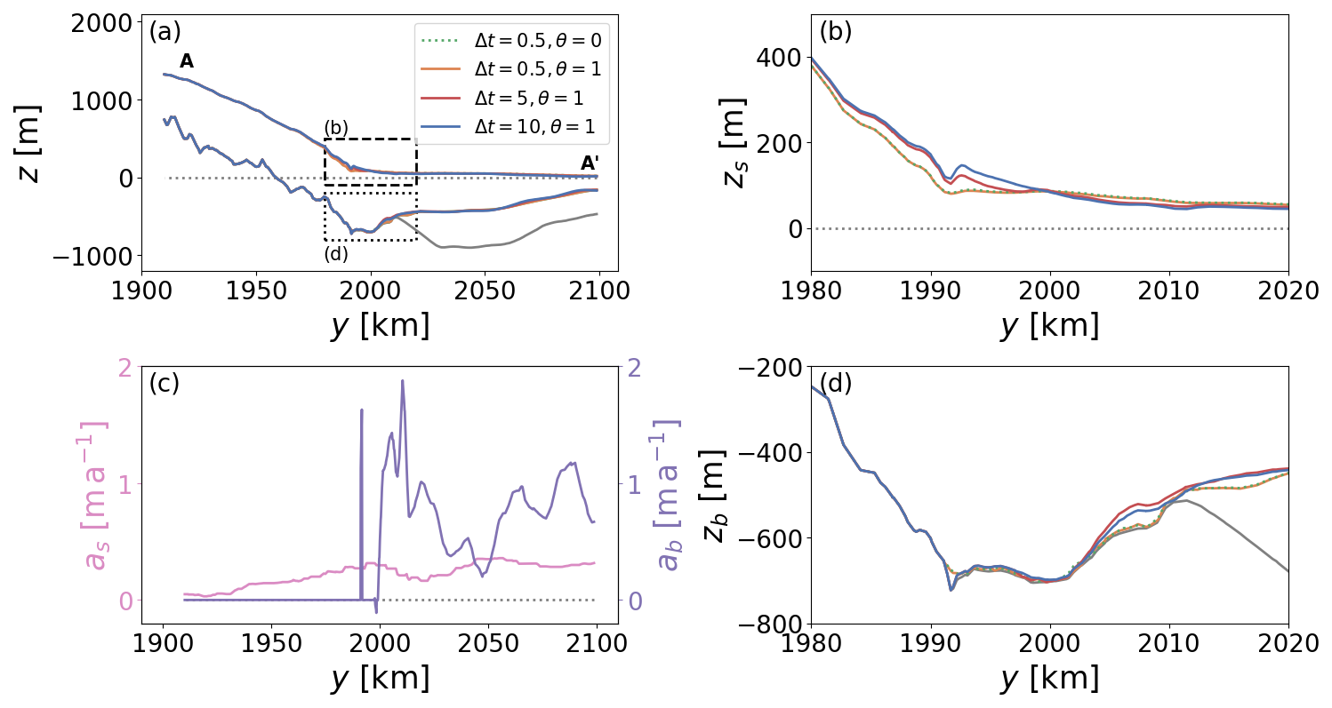
Figure 9 (a) A vertical cross-section of numerical simulations of the Ekström Ice Shelf embayment after transient evolution for 100 years. The location of the cross-section, $\mathbf{A}-{\mathbf{A}}^{\prime }$, is indicated in Fig. 8. The bed elevation is shown in grey and the sea level is shown as a black dotted line. Simulations of various time step sizes, Δt, and grounding-line horizontal mesh resolutions, Δx, are shown. (c) The surface accumulation rate, a_s (pink), and the basal melt rate, a_b (purple), are shown along the same cross-section as (a). The surface accumulation rate uses RACMO2.3p1, van den Broeke (2019). A dataset from Adusumilli et al. (2020) is used for the basal melt rates. (b, d) The upper ice surface, z_s, and the lower ice surface, z_s, in the grounding-zone as indicated by dashed and dotted boxes in (a), respectively. (c) The lower ice surface, z_b, in the grounding-zone as indicated by the box with a dotted line in (a). The grey dotted line in (b) indicates the sea level and the grey solid line in (d) indicates the bed elevation.

The three simulations that include FSSA with time step sizes of Δt=0.5, 5 and 10 years converge in a small number of iterations and result in geometries that are very similar. The FSSA simulation (θ=1) with a time step size of Δt=20 years does not converge within 100 nonlinear iterations of the Stokes solver, even in the first time step. In contrast, the only simulation without the FSSA (θ=0) to converge adequately throughout the simulation of 100 years is the simulation with a time step size of Δt=0.5. In the simulation with a time step size of Δt=5 and without the FSSA (θ=0), the Stokes solver and the free surface solvers converge for the first 7 time steps before numerical instability occurs. In the simulations with the FSSA activated and time-step sizes of 0.5, 5, and 10, the maximum horizontal velocities reach magnitudes of 196, 105, and 74 m a⁻¹. In the short simulation time, the simulations with parameter combinations of Δt=0.5 and θ=0 or θ=1 result in a retreat of the grounding line in the transect $\mathbf{A}-{\mathbf{A}}^{\prime }$ of 1225 and 770 m, respectively. The simulations with θ=1 and Δt=5 or 10 years show an advance of 8850 m and a retreat of Δt=10 m, respectively. A dip in the bedrock causing a cavity in some simulations likely explains the difference in grounding line position.

The simulations with a time step size of Δt=0.5, with and without FSSA, show very little difference in Central Processing Unit (CPU) runtime when run over 100 simulation years, with just a 0.6% difference (Fig. 10). However, when increasing the time step size to Δt=5 or Δt=10, the runtimes are 12 % and 7 % of the runtime of the Δt=0.5 with FSSA inactive (θ=0).

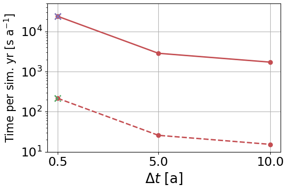
Figure 10 The average CPU time (solid line) and the wall time (dashed line) per simulation year for the Ekström Ice Shelf numerical simulations, performed over 100 simulation years starting at t=0. The crosses represent the CPU time (purple) and the wall time (green) of the unstabilised simulation. Results are shown for time step sizes of 0.5, 5, and 10 years.

6 Discussion

6.1 Efficient modelling of grounding-line dynamics

The findings of this study demonstrate that inclusion of the Free-Surface Stabilisation Algorithm (FSSA) at the ice–ocean interface significantly increases the largest numerically stable time step size of marine ice sheet simulations. In an idealised, 2D model setup, our results show that a time-step size of Δt=50 years is generally numerically stable but only accurate in phases of slow grounding line advance and retreat and that a time step size of Δt=10 years provides high accuracy throughout most of the simulations. This indicates that the dynamical changes of grounding line problems does not require the small time-steps traditionally used, and that the requirement of such small time-steps is rather due to suboptimal numerical methods with poor stability properties. However, high time-step sizes require a small time step immediately after a viscosity jump during the grounding-line retreat phase. In 100 year, 3D simulations of an embayment, a time step size of 10 years is found to be numerically stable and accurate when including the FSSA. We expect that an even higher time step size may be numerically stable after allowing further relaxation of the simulation, or correction of bed elevation datasets which are prone to inaccuracy in the grounding zones (Morlighem et al., 2020). In light of our results, we recommend the use of an adaptive time-stepping scheme when incorporating the FSSA into Stokes simulations, with a large time step size being used when little change in the velocity and geometry occurs and a small time step size when significant change in the system occurs to ensure accuracy.

The FSSA accomplishes a significant speedup in CPU runtime by predicting where the ice surface will be in the next time step, thereby mimicking an implicit time-stepping scheme when calculating the velocities using the Stokes solver. This allows anticipation and dampening of large changes in the solution, therefore allowing larger time steps to be taken. Furthermore, this work builds on an additional numerical stabilisation scheme applied to the ice–ocean interface, namely the sea spring numerical stabilisation scheme (Durand et al., 2009a). The sea spring numerical stabilisation scheme is paramount to the stability of such marine ice sheet simulations, with a time step size much lower than those used here not converging without it. The inclusion of both numerical stabilisation schemes results in the ice load and the ocean pressure being evaluated at the next time step, ensuring that a mismatch in forces at the ice–ocean interface no longer occurs. This is evident in Fig. 6, where in both the advancing and retreating phases, the simulation with the FSSA terms is further oceanward. We hypothesise that this difference during the grounding-line advance is because the simulation with the FSSA terms predicts thicker ice and therefore a higher flux, which results in faster grounding-line advance, which is in line with the theory of Schoof (2007). In the retreating case, the opposite holds. The simulation with the FSSA terms predicts thinner ice and therefore a lower ice flux and slower grounding line retreat.

6.2 Implications for ice-sheet modelling

The FSSA is an easy-to-implement approach to improve numerical stability. Since the Stokes model captures the underlying physics more accurately than simplified models, this approach leads to improved overall precision in the results. Further possibilities for a broader application of full Stokes models with the inclusion of FSSA include coupling frameworks with lower-order models (Ahlkrona et al., 2016; van Dongen et al., 2018; Seroussi et al., 2012). While FSSA enables greater numerical stability in physically complex areas such as grounding-zones, a coupling framework to a lower order model in areas where flow is less complicated will further improve model efficiency. The increased efficiency that FSSA offers has the potential to improve the applicability of simulations of ice stratigraphy, where high resolution and accurate ice flow physics are important (Henry et al., 2025; Bingham et al., 2025). Additionally, the improved efficiency has the potential for full Stokes models to be used in machine learning methods where a significant number of simulations need to be performed (Moss et al., 2025). Integrating the modelling framework with FSSA and an adaptive time-stepping scheme (Cheng et al., 2017) will allow the automated increase in efficiency while maintaining accuracy, particularly during rapid change such as grounding-line migration. While the FSSA mimicks an implicit time-stepping scheme, a fully implicit scheme would offer additional model accuracy and efficiency (Kramer et al., 2012; Bueler, 2024).

A number of problem-specific challenges remain, including the treatment of the minimum thickness constraint in combination with the FSSA, which posed a problem in initial simulations of the Ekström Ice Shelf embayment. In addition, further analysis of the discretisation schemes for application of friction and ocean pressure boundary conditions needs to be made, particularly by comparison with real-world geometries (Gagliardini et al., 2016). Further work is needed to extend well-posedness analysis and error estimation in relation to the time-dependent grounding-line contact problem (John et al., 2018; Helanow and Ahlkrona, 2018; de Diego et al., 2022). The applicability of full Stokes ice-sheet simulations will need to be tested beyond the geometries and model set up presented in this study.

7 Conclusions

In this study, we applied the Free-Surface Stabilisation Algorithm (FSSA) to the ice–ocean interface in 2D, idealised simulations and 3D, real-world simulations with the goal of improving the efficiency and applicability of complex, full Stokes models. Using the MISMIP Experiment 3a model setup (Pattyn et al., 2012), we simulated the advance and retreat of the grounding line on bed topography that transitions between pro- and retrograde slopes, capturing the characteristic hysteresis of such geometries. Including the FSSA terms on both the upper and lower ice surfaces enabled a numerically stable time step size of Δt=50 years, while a time step size of Δt=10 resolved the benchmark hysteretic behaviour of the MISMIP Exp. 3a. To demonstrate the broader applicability of the 3D, marine-terminating Stokes simulations with the FSSA, we performed simulations of the Ekström Ice Shelf embayment in Dronning Maud Land, East Antarctica. Here, we found that a time step size of Δt=10 is numerically stable and produces minimal error in geometry.

The ability to solve a coupled Stokes flow and free-surface evolution problem with time steps significantly larger than typical time step sizes of $\sim \mathrm{\Delta }t=\mathrm{0.01}-\mathrm{0.5}$ years used in ice-sheet modelling offers an alternative to simplified models which often rely on assumptions such as a hydrostatic grounding line. Combining the FSSA with an adaptive time-stepping scheme (Cheng et al., 2017) has the potential to offer improved flexibility, particularly in simulations where fine-scale dynamics or the temporal resolution of assimilated data require small time steps. The inclusion of FSSA in Stokes marine ice-sheet simulations broadens their applicability to large-scale domains, allowing an alternative to lower-order models, which neglect key physical details.