Representation of the nitrogen cycle and its coupling with the carbon cycle in ISBA (SURFEX v9) the land surface model: evaluation using two Free-Air CO₂ Enrichment experiment sites

Nitrogen (N) is a critical nutrient, that controls photosynthesis and decomposition processes. It is important to include the N cycle in the land component of climate models to improve the exchange fluxes of CO₂ between land and atmosphere. We present here the implementation of the N cycle in the CNRM land surface model, namely ISBA. We evaluate the model on two Free-Air Enrichment (FACE), experiments sites: Duke and Oak Ridge. In particular, the response to elevated CO₂ is studied. We compare the reference version without the N cycle (C) and the new version in which it is included (CN). A comparison to a multi model analysis shows encouraging results, since the computed NPP and N assimilation flux fall in the inter model range. The CN version performs better than the C version for NPP. Next, we focus on the carbon cycle by comparing simulation results to observations. The CN version improves the carbon stocks, largely overestimated by the C version. In particular, at elevated CO₂, in the CN version, photosynthesis is downregulated by the N limitation. This yields a reduction of C accumulation in soil and biomass in comparison to the C version. In the literature, diverging strategies are observed to overcome N limitation. The model reproduces well the main features but fails to represent some sites characteristics. Finally, a detailed analysis of the simulated N dynamics is presented.

1 Introduction

Climate change is driven by anthropogenic emissions of greenhouse gases, such as CO₂, to the atmosphere, which disturbs the natural carbon (C) cycle. Rising atmospheric CO₂ concentration exerts a fertilization effect by stimulating photosynthesis, causing land ecosystems to act as a C sink. This leads to an increase in C storage in terrestrial ecosystems (Pan et al., 2011; Tagesson et al., 2020; Sitch et al., 2024). This C sink plays a crucial role in mitigating the impact of human emissions, absorbing roughly one-third of the total CO₂ emissions (Friedlingstein et al., 2025). However, its long term fate is uncertain because the CO₂ fertilization effect depends on the availability of water and nutrients, and is constrained by disturbances including fires and disease (Elser et al., 2007; Fleischer and Terrer, 2022). In particular, nitrogen availability has been pointed out as a first order limiting factor on the carbon cycle (Vitousek and Howarth, 1991; Flechard et al., 2020). Nitrogen is a key nutrient for plant growth and for organic matter decomposition processes (Schlesinger, 1997; Parton et al., 1988), and long term enhanced CO₂ concentration is expected to lead to a progressive nitrogen limitation (Johnson, 2006). Reduced nitrogen availability occurs as nitrogen becomes increasingly immobilized in plant and soil organic matter, leading to lower mineral nitrogen availability for further plant uptake (Luo et al., 2004). Plants and ecosystems may partially compensate for this limitation through changes such as increased nitrogen-use efficiency (NUE), higher C : N ratios, and greater fine-root production to access additional nutrients.

Earth system models (ESMs) are used to predict future climate in response to human activity and continued CO₂ emissions (Voldoire et al., 2019). They include land surface components that may be run in an offline mode using atmospheric forcings to analyze the evolution of the land surface C sink (Sitch et al., 2024). Without representation of N constraints on the C cycle, the C uptake may be unrealistically overestimated (Wieder et al., 2015b). Therefore, modelers recently included an explicit nitrogen cycle coupled to the carbon cycle, allowing C–N interactions and feedbacks to be investigated under climate change and rising CO₂ (Goll et al., 2012; Thornton et al., 2007; De Sisto et al., 2023). On average, models including a nitrogen cycle predict a lower land carbon sink than models without one (Arora et al., 2020). Nevertheless, the range of modeled carbon stocks is wider (Stocker et al., 2025), reflecting the complexity of the processes involved (Meyerholt et al., 2020; Wieder et al., 2015a). Moreover, there is a lack of observations to constrain these models (Kou-Giesbrecht et al., 2023).

ISBA, for Interaction-Soil–Biosphere–Atmosphere, is the land surface component of the CNRM earth system model (ESM) (Séférian et al., 2019). The model is used for future projections including the Climate Model Intercomparison Project (CMIP) (Voldoire et al., 2019). It can be used interactively with the other components of the ESM, or in an offline mode using prescribed atmospheric forcings. ISBA represents the surface energy, water and carbon budgets. A dynamic C cycle is already implemented (Delire et al., 2020; Decharme et al., 2019; Morel et al., 2019; Gibelin et al., 2008) with an implicit nitrogen limitation (Yin, 2002). Despite this parametrization, the model remains too responsive to the elevated CO₂. An additional tuning was therefore implemented to obtain more realistic future C uptake projections (Delire et al., 2020). However, both of these N limitations are not process-based and feedbacks to rising CO₂ emissions are not well represented. To address this issue more mechanistically, a comprehensive nitrogen cycle needed to be implemented.

In this paper, we present the implementation of an explicit N cycle in ISBA. The approach follows developments made in other land surface models such as ORCHIDEE, JSBACH, QUINCY, JULES (Vuichard et al., 2019; Reick et al., 2021; Thum et al., 2019; Wiltshire et al., 2021). The representation of the nitrogen cycle is built consistently with the carbon cycle. C and N dynamics are coupled through stoichiometric ratios between C and N pools and by imposing nitrogen limitation on carbon assimilation and decomposition processes.

To evaluate model performance, we use data from the Free-Air CO₂ Enrichment (FACE) experiments conducted over 10 years in North America (Hendrey et al., 1999; McCarthy et al., 2010; Norby et al., 2002). These experiments, which impose an elevated atmospheric CO₂ in field conditions, provide a good framework to test the ability of the updated model to represent nutrient constraints on CO₂ fertilization (Finzi et al., 2002, 2007; Zaehle et al., 2014; Norby et al., 2010; Drake et al., 2011). We compare our model simulations to site observations and to the results of a model intercomparison exercise conducted at these two sites. We then assess the ISBA carbon cycle at the two FACE sites and evaluate the impact of adding the nitrogen cycle. Finally, we analyze the internal dynamics of the nitrogen cycle in the model and discuss further improvements.

2 Implementation of the nitrogen cycle in the ISBA land surface scheme

2.1 The carbon dynamics in ISBA

ISBA is embedded in the SURFEX modeling platform. The current version is SURFEX V9.1, described in Delire et al. (2020), Decharme et al. (2019) and Morel et al. (2019). ISBA uses a 14-layer scheme to solve soil physics (hydrology, thermodynamics, gas diffusion). The model includes the representation of 16 plant functional types (PFTs), rock, ice and bare soil. The ISBA scheme used here is ISBA-CC described in Gibelin et al. (2008). This version computes carbon cycle dynamics using 6 pools to represent plants and 7 pools for the soil organic matter. Photosynthesis is represented using a semi-empirical approach based on Jacobs (1994), implemented by Calvet et al. (1998). The scheme was modified by Joetzjer et al. (2015) for tropical vegetation. As previously stated, an implicit nitrogen limitation was implemented to regulate photosynthesis with increasing CO₂. It consists of two parameterizations: the first one acts globally to correct the model tendency to overestimate CO₂ fertilization. The second acts directly on photosynthesis by reducing the specific leaf area (SLA) with increasing CO₂, thereby constraining leaf growth and carbon assimilation (Delire et al., 2020).

The assimilated carbon is first allocated to the leaves. It is then reallocated to the other biomass pools using different empirical allometric relations (Gibelin et al., 2008). Each biomass carbon pool is associated with a respiration and a turnover rate. Soil litter and soil organic-carbon pools are represented within each soil layer, and their dynamics follow the CENTURY model of Parton et al. (1988). Latest developments include a gas module that explicitly simulates the dynamics of O₂, CO₂, and CH₄ (Morel et al., 2019) with methane related processes and vertical carbon transfers. The equations driving the carbon cycle are detailed in the Appendix A.

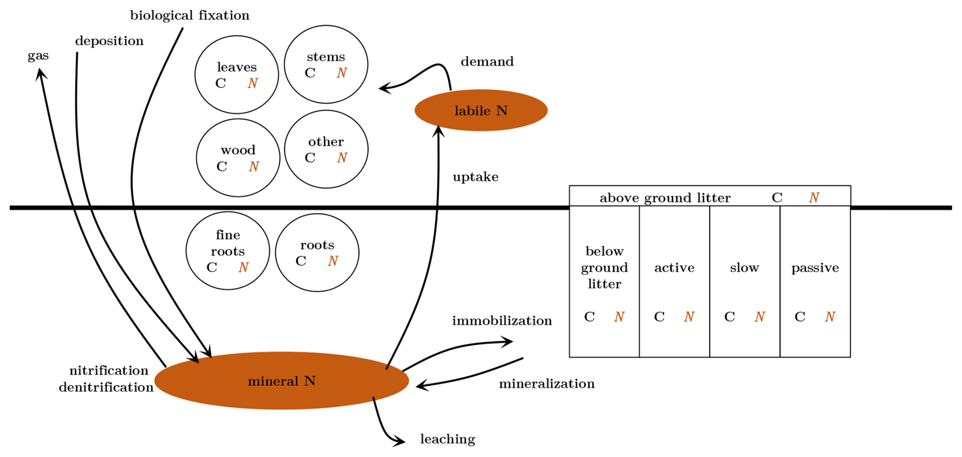
Figure 1 Schematic representation of the C and N cycle. Pools representing biomass and soil, in black existing carbon pools, in brown the newly added nitrogen pools. In italic pools which dynamics is represented implicitly. Only process linked to nitrogen cycle are represented by the arrows.

2.2 Implementation of a N cycle within the carbon dynamics in ISBA

We chose to build the nitrogen cycle consistently with the carbon cycle. Each vegetation and soil carbon pool has an associated nitrogen pool, and nitrogen decomposition fluxes follow those of carbon (Fig. 1). To reduce computational cost, these N pools and fluxes are not explicitly represented, consistent with approaches used in other land models (ISAM, Jain et al., 2009; O-CN, Zaehle and Friend, 2010; ORCHIDEE, Vuichard et al., 2019; JULES, Wiltshire et al., 2021). Instead carbon and nitrogen pools are linked by stoichiometric nitrogen-carbon ratios (N $/$ C) that are prescribed for all pools except for leaves in order to adjust vegetation response to N availability (Zaehle and Friend, 2010; Vuichard et al., 2019; Wiltshire et al., 2021). The model also explicitly describes the dynamics of a labile nitrogen pool in vegetation and a mineral nitrogen pool in soils. Soil and vegetation exchange N by an uptake flux that is a function of the mineral N availability, root distribution and plant N demand (Yang et al., 2009; Jain et al., 2009; Vuichard et al., 2019; Zaehle and Friend, 2010). Consequently, a limitation in the N mineral pool directly reduces plant NPP, and constrains the decomposition of organic matter. Gaseous exchanges with the atmosphere and leaching of mineral N are also represented.

2.3 Labile nitrogen

The labile pool of nitrogen, N_labile, is a storage pool that represents the nitrogen that is easily transported within the plant (Tegeder and Masclaux-Daubresse, 2018). N is taken up from the soil by the roots and is then redistributed to the various plant parts. Its dynamics is explicitly represented by:

$$\begin{array}{}\text{(1)}& {\displaystyle \frac{\mathrm{d}}{\mathrm{d}t}}{N}_{\mathrm{labile}}\left(t\right)=N_{\mathrm{upday}}\left(t\right)-N_{\mathrm{demand}}\left(t\right)\end{array}$$

where N_upday represents the nitrogen taken up by plants from the soil mineral reservoir (see Sect. 2.6) and N_demand is the nitrogen needed to build plant tissues. Because the C allocation scheme in ISBA is built as a cascade through the biomass pools with multiple outcomes (see Appendix A), the computation of the N needed to fulfill tissue growth is diagnosed by comparing the total biomass before and after C allocation and applying the corresponding N $/$ C ratio. However, this diagnosed flux needs to be corrected by turnover because the change in total biomass results from both tissue growth and turnover while only growth implies a N demand.

$$\begin{array}{}\text{(2)}& N_{\mathrm{demand}}^{*}={\displaystyle \frac{\mathrm{1}}{\mathrm{\Delta }t}}\sum _{x=\mathrm{1}}^{\mathrm{6}}\left[B_x^{*}(t+\mathrm{\Delta }t)-B_x\left(t\right)\right]\times N{C}_{B_x}+N_{\mathrm{turn}}^{*}\left(t\right)\end{array}$$

where $N{C}_{B_x}$ is the N $/$ C ratio of the biomass pool x and $N_{\mathrm{turn}}^{*}$ is the N lost by turnover. To render the known N translocation of N from leaf to plant during senescence (Norby and Iversen, 2006; Finzi et al., 2002), the N turnover flux is reduced by a fraction that is directed from the leaf pool to the storage pool before leaf fall. This results in marked difference between C turnover and N turnover. This has the effect of decorrelating C and N turnover fluxes. $N_{\mathrm{turn}}^{*}$ is expressed as:

$$\begin{array}{}\text{(3)}& N_{\mathrm{turn}}^{*}\left(t\right)=\sum _{x=\mathrm{1}}^{\mathrm{6}}\left(\mathrm{1}-f_{\mathrm{trans},x}\right)M_x\left(t\right)N{C}_{B_x}\end{array}$$

Vuichard et al. (2019)Zaehle and Friend (2010)Wiltshire et al. (2021)Sparks et al. (2008)Norby et al. (2010)Thum et al. (2019)Reick et al. (2021)Reick et al. (2021)Thum et al. (2019)Xu-Ri and Prentice (2008)Xu-Ri and Prentice (2008)Thum et al. (2019)Thum et al. (2019)Thum et al. (2019)Thum et al. (2019)Zaehle and Friend (2010)Zaehle and Friend (2010)Zaehle and Friend (2010); Kronzucker et al. (1996)

Table 1 Parameters used for the implementation of the N cycle.

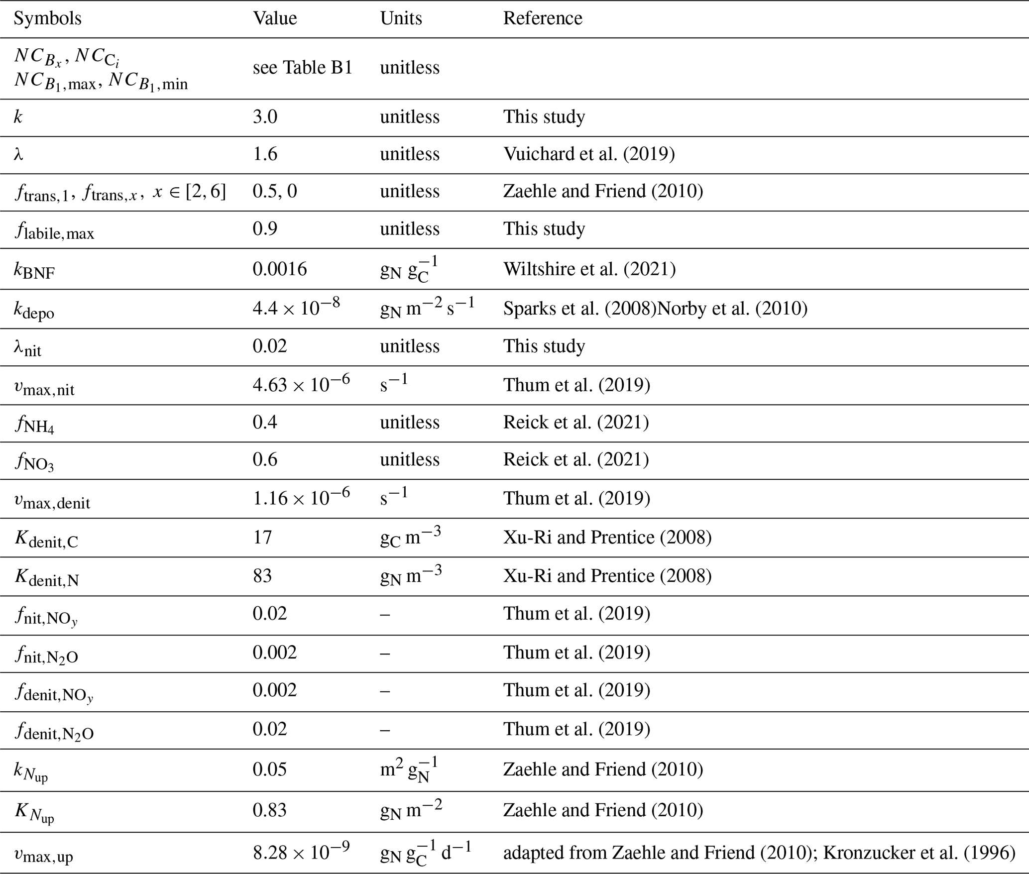
where f_trans,x is the fraction of nitrogen from pool x that is translocated (see Table 1) and M_x the turnover rate of the C pool x. ^* denotes potential fluxes before N limitation that is described in Sect. 2.4. In these last 2 equations, $N{C}_{B_x}$ is time dependent for leaves and prescribed for all other pools (see Sect.2.5). N demand can be positive: nitrogen is needed to meet carbon demand. However, the biomass cascade in the model is build so that carbon is transferred from metabolic pools (high N $/$ C) to more ligneous pools (low N $/$ C). As a consequence, the N demand can also be negative. In this case, the surplus of nitrogen is transferred to the labile pool. Similarly to the C allocation scheme, the dynamics of N_labile is computed once a day.

2.4 Nitrogen limitation in biomass

In response to N limitation, the photosynthesis is reduced which slows down tissue growth. In addition, the plant limit N losses by readsorbing more N during senescence. In the model, both strategies are implemented sequentially. The first step is to limit C assimilation. This is implemented by computing the C allocation scheme twice. The first time, the C allocation is computed considering infinite N supply. This gives the potential $N_{\mathrm{demand}}^{*}$ from Eqs. (2) and (3) that is compared to the available labile N to compute the limitation parameter, η_lim,assim, following Zaehle and Friend (2010):

$$\begin{array}{}\text{(4)}& {\mathit{\eta }}_{\lim ,\mathrm{assim}}=\min \left(\mathrm{1},{\displaystyle \frac{f_{\mathrm{labile},\max }{N}_{\mathrm{labile}}}{N_{\mathrm{demand}}^{*}\mathrm{\Delta }t}}\right)\end{array}$$

where $f_{\mathrm{labile},\max }=\mathrm{0.9}$ is a limit to empty at most 90 % of the labile pool. This limitation is immediately applied to the daily net carbon assimilation by leaves during the second round of computation of C allocation. $A_{\mathrm{1}}\left(t\right)={\mathit{\eta }}_{\lim ,\mathrm{assim}}{A}_{\mathrm{1}}^{*}\left(t\right)$. This updates all the biomass pools and the actual N demand.

$$\begin{array}{}\text{(5)}& N_{\mathrm{demand}}={\displaystyle \frac{\mathrm{1}}{\mathrm{\Delta }t}}\sum _{x=\mathrm{1}}^{\mathrm{6}}\left[B_x(t+\mathrm{\Delta }t)-B_x\left(t\right)\right]\times N{C}_{B_x}+N_{\mathrm{turn}}^{*}\left(t\right)\end{array}$$

The limitation may persist. The second step is then to increase retranslocation from leaves to the labile pool, as it has been done in the FUN model developed by Fisher et al. (2010). A correction is applied to the nitrogen turnover flux if there is no sufficient N labile to support it. The corrective factor, f_corr, is computed as the ratio of the maximum quantity that can be removed from the labile pool ($f_{\mathrm{labile},\max }{N}_{\mathrm{labile}}-N_{\mathrm{demand}}$) and the potential turnover flux $N_{\mathrm{turn}}^{*}$.

$$\begin{array}{}\text{(6)}& f_{\mathrm{corr}}=\min \left(\mathrm{1},{\displaystyle \frac{f_{\mathrm{labile},\max }{N}_{\mathrm{labile}}-N_{\mathrm{demand}}}{N_{\mathrm{turn}}^{*}}}\right)\end{array}$$

The actual turnover is then $N_{\mathrm{turn}}=f_{\mathrm{corr}}{N}_{\mathrm{turn}}^{*}$.

2.5 Nitrogen carbon ratio

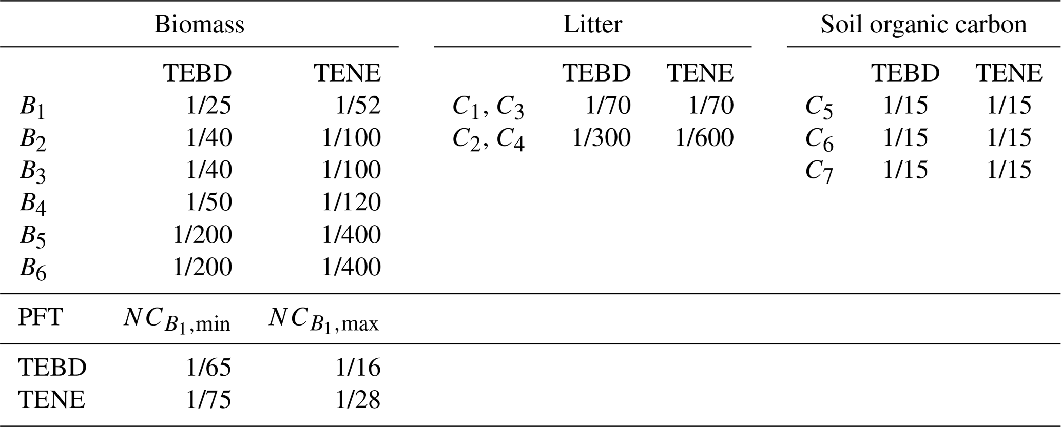
The nitrogen-carbon ratio evolves during the plant development and also in response to environmental constraints (Vitousek et al., 1988). It has been observed in general that (i) structural elements such as branches, bark or heartwood contain less nitrogen than leaves. (ii) Litter is N poor compared to vegetation biomass and soil organic carbon. As a first approximation, we assumed in the model the ratio to be constant for all pools except for leaves. We prescribe a PFT-dependent value adapted from literature (Vitousek et al., 1988; White et al., 2000; Kattge et al., 2020). The ratio associated with each carbon pool is denoted by $N{C}_{B_x}$, for biomass pool B_x and $N{C}_{C_i}$ for soil carbon pool C_i. Table B1 summarizes values used in the model. The leaf ratio, $N{C}_{B_{\mathrm{1}}}$, varies in order to adjust the system to the nitrogen availability. Initial value is taken according literature. Then, it increases when the nitrogen supply matches the potential total demand $N_{\mathrm{labile}}>N_{\mathrm{demand}}^{*}$, otherwise it decreases. Minimum and maximum values are set to avoid unrealistic ratios (see Table B1). Variations of $N{C}_{B_{\mathrm{1}}}$ are described by Eq. (7), adapted from Vuichard et al. (2019).

$$\begin{array}{}\text{(7)}& \begin{array}{rl}& N{C}_{B_{\mathrm{1}}}(t+\mathrm{\Delta }t)=\\ & \left\{\begin{array}{ll}{N}_{\mathrm{labile}}<N_{\mathrm{demand}}^{*}:& N{C}_{B_{\mathrm{1}}}\left(t\right)\times \max \left(\frac{N{C}_{B_{\mathrm{1}},\min }}{N{C}_{B_{\mathrm{1}}}\left(t\right)},\mathrm{1}-\mathrm{0.25}\times {\mathit{\gamma }}_{NC}\right)\\ N_{\mathrm{labile}}>N_{\mathrm{demand}}^{*}:& N{C}_{B_{\mathrm{1}}}\left(t\right)\times \min \left(\frac{N{C}_{B_{\mathrm{1}},\max }}{N{C}_{B_{\mathrm{1}}}\left(t\right)},\mathrm{1.25}-\mathrm{0.25}\times {\mathit{\gamma }}_{NC}\right)\end{array}\right.\end{array}\end{array}$$

where γ_NC dampens the variation according to:

$$\begin{array}{}\text{(8)}& {\mathit{\gamma }}_{NC}=\exp \left(-{\left[\mathit{\lambda }\times {\displaystyle \frac{N{C}_{B_{\mathrm{1}},\max }-N{C}_{B_{\mathrm{1}}}\left(t\right)}{N{C}_{B_{\mathrm{1}},\max }-N{C}_{B_{\mathrm{1}},\min }}}\right]}^k\right).\end{array}$$

The parameters λ=1.6 and k=3.0 are chosen to adjust the dampening effect, which must allow the NC ratio to reach its boundary values.

2.6 Soil mineral nitrogen

Mineral (inorganic) N may be found as two soluble species in the soil: ${\mathrm{NH}}_{\mathrm{4}}^{+}$ and ${\mathrm{NO}}_{\mathrm{3}}^{-}$ (Schlesinger, 1997). Nitrogen enters the soil system by biological N fixation (BNF), N_BNF, and by deposition, N_depo. Both are complex processes (Cleveland et al., 1999; Bellenger et al., 2020; Galloway et al., 2004; Lamarque et al., 2011) that are simplified and supposed to directly supply the mineral pool (see Sect. 2.6.1). Mineral nitrogen undergoes chemical reactions (nitrification and denitrification) during which N is lost to the atmosphere as gas, N_gas. N is also lost due to leaching towards river and oceans, N_leaching and by plants to fulfill growth, N_up. Decomposition processes are releasing nitrogen, but micro-organisms requires nitrogen to carry out their tasks. This is denoted by net mineralization, N_netmin. We represent the two ion species as one mineral pool N_min with associated fractions of ${\mathrm{NH}}_{\mathrm{4}}^{+}$ ($f_{{\mathrm{NH}}_{\mathrm{4}}}$) and ${\mathrm{NO}}_{\mathrm{3}}^{-}$ ($f_{{\mathrm{NO}}_{\mathrm{3}}}=\mathrm{1}-f_{{\mathrm{NH}}_{\mathrm{4}}}$), similarly to Reick et al. (2021). The soil N mineral pool is vertically discretized and its dynamics is computed on the same vertical grid as the soil water, temperature and carbon. Mineral N dynamics is described for each soil layer l by:

$$\begin{array}{}\text{(9)}& \begin{array}{rl}{\displaystyle \frac{\mathrm{d}}{\mathrm{d}t}}{N}_{\min ,l}\left(t\right)& =N_{\mathrm{BNF}}{f}_{\mathrm{water},l}+N_{\mathrm{depo}}{f}_{\mathrm{water},l}-N_{\mathrm{gas},l}\\ & -N_{\mathrm{leaching},l}-N_{\mathrm{up},l}+N_{\mathrm{netmin},l}.\end{array}\end{array}$$

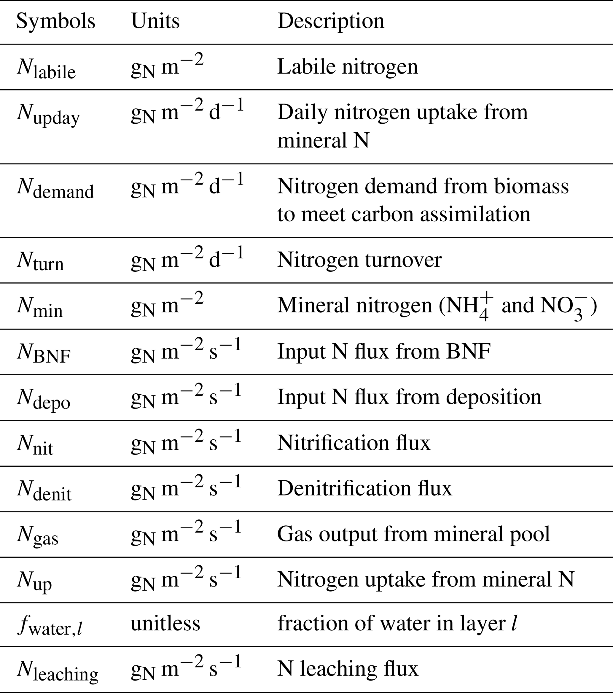
Variables added to represent the soil N dynamics are summarized in Table E1, and the fluxes are detailed in the following sections.

2.6.1 External input

Biological fixation

For simplification, the various sources of biological fixation are not detailed. The idea is to model the entry of nitrogen without describing the complexity of the process. Based on Cleveland et al. (1999) approach, which states that biological fixation is proportional to NPP, the land surface model JULES used a linear correlation between BNF and NPP (Wiltshire et al., 2021). The same formulation is used here:

$$\begin{array}{}\text{(10)}& N_{\mathrm{BNF}}=k_{\mathrm{BNF}}\mathrm{NPP},\end{array}$$

where k_BNF is the rate of fixation in g_N g${}_{\mathrm{C}}^{-\mathrm{1}}$ and is set to match the global value of BNF observed per year (100 Tg_N yr⁻¹, Galloway et al., 2004).

Deposition

Deposition is computed using a fixed rate k_depo in g_N m² s⁻¹ to match the annual deposition flux observed. In this study, we take observed values from Sparks et al. (2008); Norby et al. (2010) (see Table 1). Hence,

$$\begin{array}{}\text{(11)}& N_{\mathrm{depo}}=k_{\mathrm{depo}}.\end{array}$$

The deposition is added to the mineral pool and is supposed to be immediately accessible for the biomass.

Approximation of diffusivity

The ${\mathrm{NH}}_{\mathrm{4}}^{+}$ and ${\mathrm{NO}}_{\mathrm{3}}^{-}$ ions that form the N mineral pool are soluble and diffuse in water (Schlesinger, 1997). To mimic the result of this diffusion that is not currently represented in ISBA, the BNF and deposition input fluxes are spread per layer according to the water vertical profile:

$$\begin{array}{}\text{(12)}& f_{\mathrm{water},l}={\displaystyle \frac{w_{\mathrm{g},l}\mathrm{\Delta }{z}_l}{\sum _{l=\mathrm{1},l_{\mathrm{bottom}}}{w}_{\mathrm{g},l}\mathrm{\Delta }{z}_l}}\end{array}$$

where w_g,l is the soil liquid water content of layer l in m³ m⁻³, Δz_l is the layer thickness in m and l_bottom the last soil layer.

2.6.2 Gas losses

Numerous chemical reactions occur in the soil, transforming nitrogen species from one form into another. The two main reactions are nitrification and denitrification and are both represented in the model. During nitrification, ${\mathrm{NH}}_{\mathrm{4}}^{+}$ is oxidized in ${\mathrm{NO}}_{\mathrm{3}}^{-}$ and denitrification transforms ${\mathrm{NO}}_{\mathrm{3}}^{-}$ into N₂ that is released to the atmosphere. During these reactions, other species are emitted as by-products such as N₂O and NO, both being greenhouse gases of interest. We model autotrophic nitrification that occurs under aerobic conditions and denitrification carried out by denitrifier under anaerobic conditions. Both reactions can take place at the same time and place because the soil contains micropores that have different water saturation status.

As a first step, the aim is to quantify the inorganic losses as gases. Later, diffusion of gases will be described and each gas species will be tracked down following the work of Morel et al. (2019). The modeling of gas losses is based on the QUINCY model (Thum et al., 2019). We divide the soil by defining an anaerobic fraction that is a key parameter to represent denitrification and nitrification as discussed in Schlüter et al. (2025). In this model, we will use a simplified scheme that does not account for the soil heterogeneity. Since we have access to the simulated concentration profile in the soil of O₂, we follow a similar approach of Li et al. (2000). We modify the function used in this paper according to Thum et al. (2019) to account for a more abrupt transition between anaerobic and aerobic.

$$\begin{array}{}\text{(13)}& f_{\mathrm{anaero},l}=\exp \left(-{\mathit{\lambda }}_{\mathrm{nit}}\times {\displaystyle \frac{p_{{\mathrm{O}}_{\mathrm{2}},\mathrm{soil},l}}{p_{\mathrm{soil},l}}}\right)\end{array}$$

where $p_{{\mathrm{O}}_{\mathrm{2}},\mathrm{soil},l}$ is the O₂ partial pressure in soil at layer l and p_soil,l, the total soil pressure at layer l. O₂ pressure is derived from the O₂ concentration computed by using the gas module implemented in the latest ISBA version as described by Morel et al. (2019). The equation is designed to suppress nitrification below a partial pressure of oxygen of 0.5 % relatively to the soil pressure (Li et al., 2000), Table 1 references parameters units and values.

Nitrification

Nitrification is represented as a fixed maximum rate, v_max,nit, of ${\mathrm{NH}}_{\mathrm{4}}^{+}$ being transformed into ${\mathrm{NO}}_{\mathrm{3}}^{-}$. The reaction takes place in the aerobic part of soil, ($\mathrm{1}-f_{\mathrm{anaero},l}$). The flux is corrected by temperature and soil moisture functions described in Appendix C1.

$$\begin{array}{}\text{(14)}& N_{\mathrm{nit},l}=v_{\max ,\mathrm{nit}}{f}_{{\mathrm{NH}}_{\mathrm{4}}}{N}_{\min ,l}\left(\mathrm{1}-f_{\mathrm{anaero},l}\right)f\left({\mathit{\theta }}_l\right)f\left(T_l\right)\end{array}$$

Parameters used are referenced in Table 1.

Denitrification

According to Li et al. (2000) and Thum et al. (2019), denitrification can be modeled as Michaelis-Menten functions of the ${\mathrm{NO}}_{\mathrm{3}}^{-}$ and soluble C pools (corresponding in ISBA to the active carbon pool C₁). There is a fixed maximum rate of mineral N denitrified v_max,denit, corrected by a function of temperature f(T_l) described in Appendix C2.

$$\begin{array}{}\text{(15)}& \begin{array}{rl}{N}_{\mathrm{denit},l}=& v_{\max ,\mathrm{denit}}f\left(T_l\right){\displaystyle \frac{C_{\mathrm{1},l}}{K_{\mathrm{denit},\mathrm{C}}\mathrm{\Delta }{z}_l+C_{\mathrm{1},l}}}\\ & {\displaystyle \frac{f_{{\mathrm{NO}}_{\mathrm{3}}}{N}_{\min ,l}}{K_{\mathrm{denit},\mathrm{N}}\mathrm{\Delta }{z}_l+f_{{\mathrm{NO}}_{\mathrm{3}}}{N}_{\min ,l}}}{f}_{\mathrm{anaero},l}{f}_{{\mathrm{NO}}_{\mathrm{3}}}{N}_{\min ,l}\end{array}\end{array}$$

Parameters are described in Table 1.

Gas output

During both the nitrification and denitrification processes, NO_y and N₂O gases are lost as by-products. Denitrification ultimately releases N₂. Prescribed fractions derived from observations (Khalil et al., 2004; Parton et al., 1996), are used to compute the flux of each gas:

$$\begin{array}{}\text{(16)}& \begin{array}{rl}& N_{{\mathrm{NO}}_y,l}=f_{\mathrm{nit},{\mathrm{NO}}_y}{N}_{\mathrm{nit},l}+f_{\mathrm{denit},{\mathrm{NO}}_y}{N}_{\mathrm{denit},l}\\ & N_{{\mathrm{N}}_{\mathrm{2}}\mathrm{O},l}=f_{\mathrm{nit},{\mathrm{N}}_{\mathrm{2}}\mathrm{O}}{N}_{\mathrm{nit},l}+f_{\mathrm{denit},{\mathrm{N}}_{\mathrm{2}}\mathrm{O}}{N}_{\mathrm{denit},l}\\ & N_{{\mathrm{N}}_{\mathrm{2}},l}=\left(\mathrm{1}-f_{\mathrm{denit},\mathrm{NO}}-f_{\mathrm{denit},{\mathrm{N}}_{\mathrm{2}}\mathrm{O}}\right)N_{\mathrm{denit},l}.\end{array}\end{array}$$

This is a simplified representation. The amount of N₂O produced is linked to the microbial community in the soil. More complex models explicitly describe the nitrifiers and denitrifiers population dynamics (Li et al., 2000; Ma et al., 2022). The ratio can also be temperature and humidity dependent such as proposed by Xu-Ri and Prentice (2008). As a result, the total gas loss from the mineral pool to the atmosphere comes from the by-products of the nitrification reaction and the entire denitrification flux:

$$\begin{array}{}\text{(17)}& N_{\mathrm{gas},l}=f_{\mathrm{nit},{\mathrm{NO}}_y}{N}_{\mathrm{nit},l}+f_{\mathrm{nit},{\mathrm{N}}_{\mathrm{2}}\mathrm{O}}{N}_{\mathrm{nit},l}+N_{\mathrm{denit},l}.\end{array}$$

2.6.3 Nitrogen leaching

We assume that nitrogen is leaching at the same rate k_drain as water drainage:

$$\begin{array}{}\text{(18)}& k_{\mathrm{drain}}={\displaystyle \frac{F_{\mathrm{drain}}}{w_{\mathrm{g},l_{\mathrm{bottom}}}{\mathit{\rho }}_{\mathrm{w}}\mathrm{\Delta }{z}_{l_{\mathrm{bottom}}}}}\end{array}$$

where F_drain is the drainage flux at the bottom of the soil column in kg m⁻² s⁻¹, $w_{\mathrm{g},l_{\mathrm{bottom}}}$ the water content of the bottom soil layer in m³ m⁻³, ρ_w the water density in kg m⁻³ and $\mathrm{\Delta }{z}_{l_{\mathrm{bottom}}}$ the bottom soil layer thickness. Total N loss is then k_drainN_min. To compensate the fact that the vertical transport of N_min is not represented, the N leaching flux is removed from each layer:

$$\begin{array}{}\text{(19)}& N_{\mathrm{leaching},l}=k_{\mathrm{drain}}{N}_{\min ,l}.\end{array}$$

2.6.4 Nitrogen uptake

$$\begin{array}{}\text{(20)}& \begin{array}{rl}{N}_{\mathrm{up},l}=& v_{\max ,\mathrm{up}}{N}_{\min ,l}\left(k_{\mathrm{Nup}}+{\displaystyle \frac{\mathrm{1}}{N_{\min ,l}+K_{N_{\mathrm{up}}}}}\right)f\left(T_l\right)\\ & f\left(N{C}_{\mathrm{leaf}}\right)f_{\mathrm{root},l}{B}_{\mathrm{4}}.\end{array}\end{array}$$

Plant nitrogen uptake is described by Eq. (20) following work of Zaehle and Friend (2010). The uptake flux is a growing function of the roots density (f_root,lB₄ with f_root,l the root fraction in layer l) and has a Michaelis–Menten dependency on the size of the mineral pool. The flux is computed for each soil layer l. Its temperature dependency f(T_l) is a Q₁₀ function as for the decomposition processes. The flux is a function of the plant N status, described by Eq. (21): the more nitrogen content in the plant the less nitrogen uptake and vice-versa.

$$\begin{array}{}\text{(21)}& f\left(N{C}_{B_{\mathrm{1}}}\right)=\max \left(\mathrm{0},{\displaystyle \frac{N{C}_{B_{\mathrm{1}}}\left(t\right)-N{C}_{B_{\mathrm{1}},\max }}{N{C}_{B_{\mathrm{1}},\min }-N{C}_{B_{\mathrm{1}},\max }}}\right)\end{array}$$

Soil dynamics is computed at the model timestep, therefore the uptake flux from soil layer l N_up,l is summed throughout the day to be used for the biomass dynamics. It is also summed through all layers. N_upday is the resulting flux defined by,

$$\begin{array}{}\text{(22)}& N_{\mathrm{upday}}=\sum _t\sum _l{N}_{\mathrm{up},l,t}\mathrm{\Delta }t.\end{array}$$

2.6.5 Net mineralization

During the decomposition process, nitrogen contained in the plant tissue is mineralized. Conversely, micro-organisms require nitrogen to carry out their decomposition tasks. In particular, the decomposition of litter, which is poor in nitrogen, immobilizes mineral nitrogen (Schlesinger, 1997). In the model, this is represented by a nitrogen flux associated with each carbon decomposition flux following Parton et al. (1988). The flux can be positive if nitrogen is mineralized, corresponding to a carbon transfer from a high nitrogen content pool to a pool with a lower nitrogen content. If the flux is negative, nitrogen is immobilized from the mineral pool to support the decomposition process. This happens when carbon is transferred from a low nitrogen content pool to a higher nitrogen content pool. Respiration due to decomposition is associated to mineralization of nitrogen. Nitrogen fluxes associated to carbon decomposition are the following:

• $F_{B_x,L_{\mathrm{surf}}}$ is the aboveground biomass pool turnover ($B_x,x\in \mathit{\{}\mathrm{1},\mathrm{2},\mathrm{3},\mathrm{5}\mathit{\}}$) becoming the surface litter (C₁ and C₂). This flux is divided on the first four soil layers using a weight ratio $w_{N_{\min ,l}}$ computed by Eq. (24).

• $F_{B_x,L_{\mathrm{soil}}}$ is the belowground biomass pool (roots) turnover ($B_x,x\in \mathit{\{}\mathrm{4},\mathrm{6}\mathit{\}}$) becoming the soil litter (C₃ and C₄). The turnover is distributed to the soil according the root profile.

• $F_{L_{\mathrm{surf},\mathrm{SOC}}}$ is the decomposition from surface litter (C₁ and C₂) to SOC pools ($C_i,i\in \mathit{\{}\mathrm{5},\mathrm{6},\mathrm{7}\mathit{\}}$). This flux is divided on the first 4 soil layers using a weight ratio $w_{N_{\min ,l}}$ computed by Eq. (24).

• $F_{L_{\mathrm{soil},\mathrm{SOC},l}}$ is the decomposition in layer l from soil litter (C₃ and C₄) to SOC pools ($C_i,i\in \mathit{\{}\mathrm{5},\mathrm{6},\mathrm{7}\mathit{\}}$)

• F_SOC,l is the decomposition in layer l of SOC pools ($C_i,i\in \mathit{\{}\mathrm{5},\mathrm{6},\mathrm{7}\mathit{\}}$).

Net mineralization is the resultant flux computed by:

$$\begin{array}{}\text{(23)}& \begin{array}{rl}{N}_{\mathrm{netmin},l}& =F_{B_x,L_{\mathrm{surf}}}{w}_{N_{\min ,l}}+F_{B_x,L_{\mathrm{soil}}}{f}_{\mathrm{root},l}\\ & +F_{L_{\mathrm{surf},\mathrm{SOC}}}{w}_{N_{\min ,l}}+F_{L_{\mathrm{soil},\mathrm{SOC},l}}+F_{\mathrm{SOC},l}\end{array}\end{array}$$

where $w_{N_{\min ,l}}$ is the weight ratio to separate the aboveground biomass turnover and the surface litter decomposition to the first 4 soil layers:

$$\begin{array}{}\text{(24)}& w_{N_{\min ,l}}={\displaystyle \frac{N_{\min ,l}}{\sum _{k=\mathrm{1}}^{\mathrm{4}}{N}_{\min ,k}}}.\end{array}$$

Further details on the computation of this fluxes can be found in Appendix D.

2.6.6 Soil nitrogen limitation

Each flux that removes N from the N mineral pool can be limited if there is not enough mineral N to support it. Due to the code construction, net mineralization is computed first, and is thus prioritized in case of N deficit. This is not in contradiction with observations (Finzi et al., 2002). N limitation on the decomposition process depends on the decomposition process considered:

1. Decomposition of biomass: the code is constructed so that decomposition of biomass should lead to N mineralization. Indeed, N $/$ C ratios of biomass pools are higher than the litter ones. However, when N_labile is very low, N turnover may be strongly reduced by translocation (see Sect. 2.4) leading to an effective N $/$ C ratio for the turnover flux that can be lower than N $/$ C ratio of litter. This can lead to a critical situation if there is not enough mineral N to support it. This situation is in practice very rare. We chose for numerical reasons to allow for a provisional N deficit that is retrieved from the N mineral pool as soon as possible during the next time steps to ensure a closed budget.

2. Other decomposition processes: the immobilization flux F is computed from the potential flux F^* by applying the limitation as $F=F^{*}{\mathit{\eta }}_{\lim ,\mathrm{decomp},l}$, where

   $$\begin{array}{}\text{(25)}& {\mathit{\eta }}_{\lim ,\mathrm{decomp},l}=\min \left(\mathrm{1.0},{\displaystyle \frac{N_{\min ,l}}{F^{*}}}\right).\end{array}$$

   The limitation is also applied to the carbon decomposition flux $F_{\mathrm{oxic},i,l}$ to maintain the N $/$ C ratio of the pool. For decomposition of surface litter the limitation is modified to compare the flux to the N content of the first four layers.

   $$\begin{array}{}\text{(26)}& {\mathit{\eta }}_{\lim ,\mathrm{decomp}}=\min \left(\mathrm{1.0},{\displaystyle \frac{\sum _{k=\mathrm{1}}^{\mathrm{4}}{N}_{\min ,k}}{F^{*}}}\right)\end{array}$$

The limitation is then done on the other mineral N output fluxes by comparing the mineral N available and the sum of all fluxes that empty the mineral N pool:

$$\begin{array}{}\text{(27)}& {\mathit{\eta }}_{\lim ,\mathrm{soil},l}=\min \left(\mathrm{1.0},{\displaystyle \frac{N_{\min ,l}}{\mathrm{\Delta }t\left(N_{\mathrm{gas},l}^{*}+N_{\mathrm{up},l}^{*}+N_{\mathrm{leaching},l}^{*}\right)}}\right).\end{array}$$

Similarly, the final output fluxes are computed by applying the limitation to the potential output fluxes N^*.

3 Methods

3.1 Evaluation sites: Duke forest and Oak Ridge

The model is evaluated on two Free-Air CO₂ enrichment (FACE), experiment sites located in North America: Duke and Oak Ridge forests. Figure 2 exhibits the mean seasonal temperature and precipitation at Duke and Oak Ridge. Both sites present a similar climate. The average annual temperature and precipitation are: 15.5 °C and 1140 mm at Duke (Lichter et al., 2005) and 13.9 °C and 1371 mm at Oak Ridge (Johnson et al., 2004).

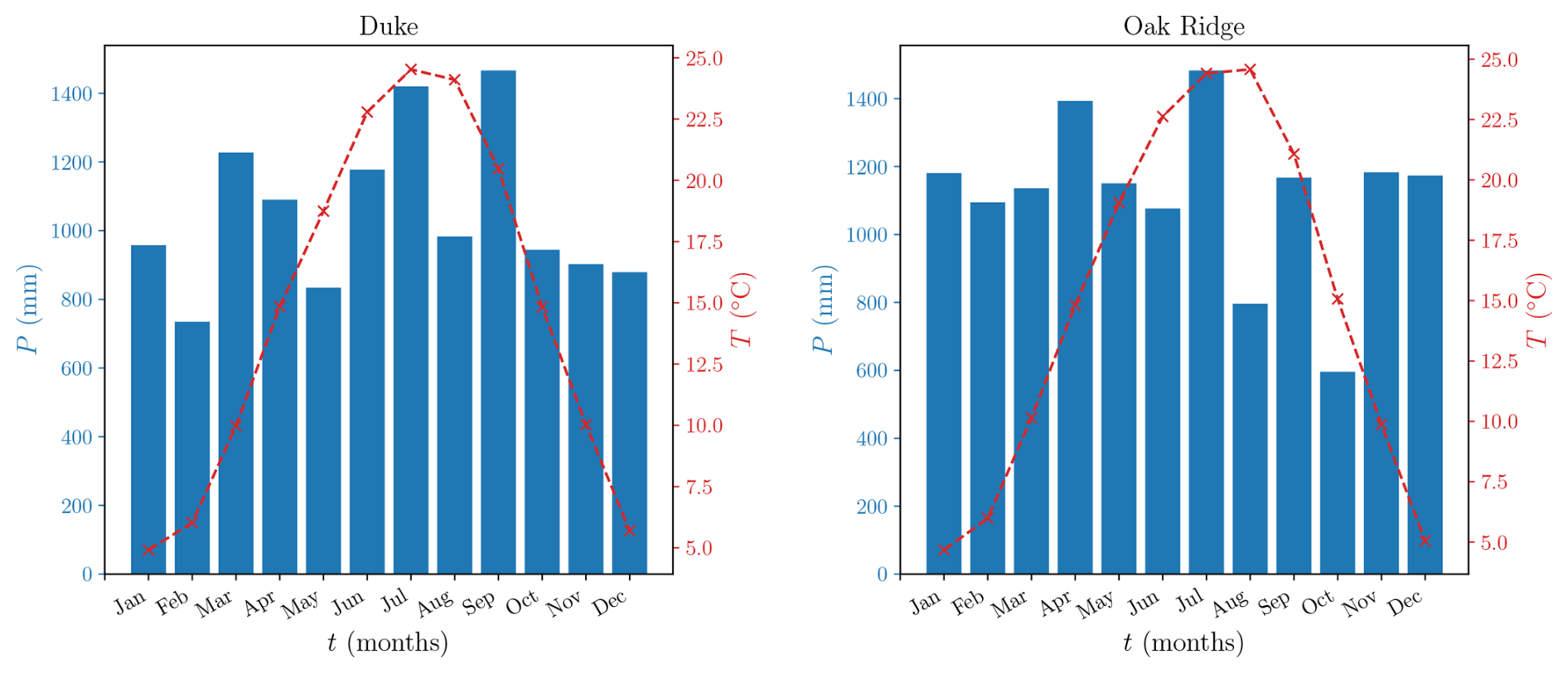
Figure 2 Mean seasonal temperature (red dashed line) and precipitation (blue bars) at both sites during the experiment period: 1996–2007 at Duke (left panel) and 1998–2008 at Oak Ridge (right panel).

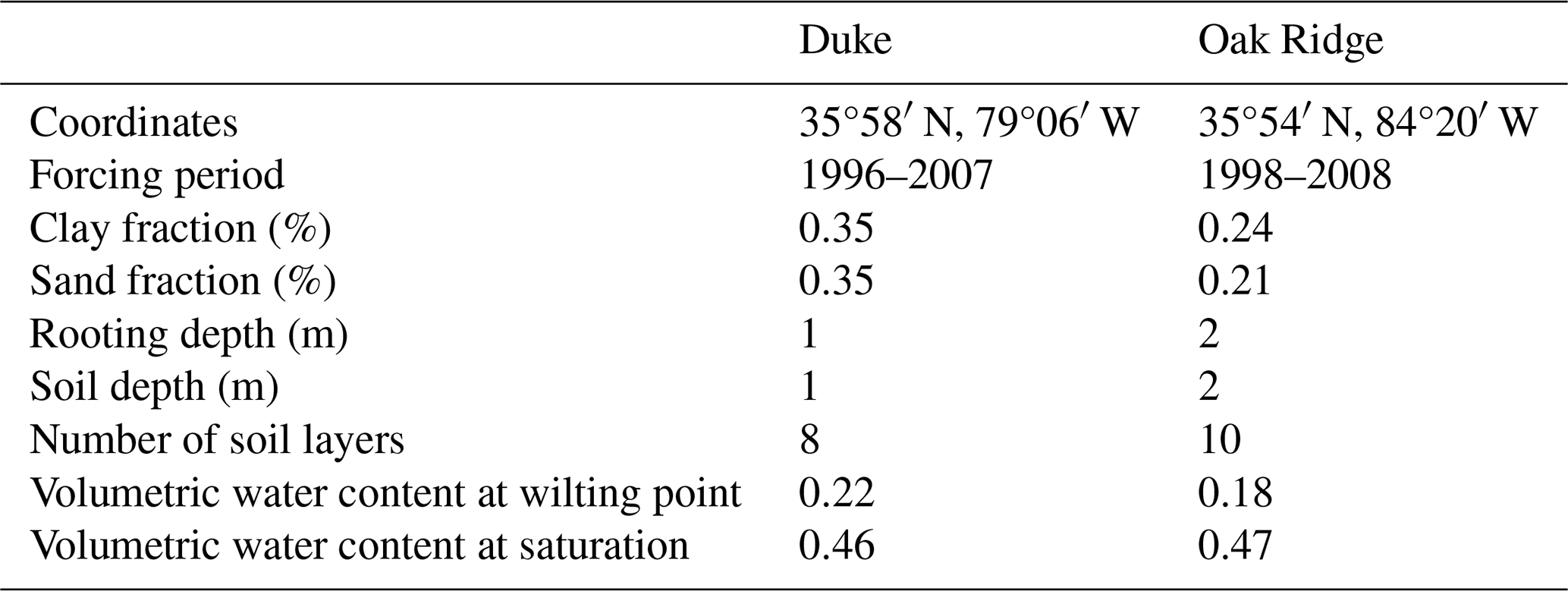
The Duke experiment was conducted in a pine forest in North Carolina (35°58^′ N, 79°06^′ W). The stand is composed of 92 % loblolly pine (Pinus taeda), with sub-dominant sweetgum and yellow poplar trees, and 48 other woody plant species (Hamiton et al., 2002). The forest was established in 1983 and the experiment began in 1996 (Lichter et al., 2005). Six circular plots, each 30 m in diameter, were studied. Half were used as control plots and were exposed to ambient CO₂ concentration, (aCO₂: 350 ppm), while the other three received elevated CO₂ concentration (eCO₂: 571 ppm) (Hamiton et al., 2002).

Oak Ridge forest is composed of sweetgum (Liquidambar styraciflua L.) and is located in Tennessee (35°54^′ N, 84°20^′ W). Trees were planted in 1988, and the experiment began in 1997 (Norby and Iversen, 2006). The plots have a diameter of 25 m. There are two control (aCO₂: 390 ppm) and three elevated CO₂ plots (eCO₂: 542 ppm) (Jastrow et al., 2005).

For both sites, regular measurements of annual carbon fluxes, biomass pools, and soil carbon content can be found in the literature (Zaehle et al., 2014; McCarthy et al., 2010; Norby et al., 2002; Lichter et al., 2005; Jastrow et al., 2005; Johnson et al., 2004) and have been used to compare simulation results with observations.

3.2 Simulation setup and protocol

Only the dominant tree specie is modeled: pine for Duke and sweetgum for Oak Ridge. We used the corresponding ISBA PFT: temperate evergreen needle-leaved trees for Duke and temperate broadleaved deciduous trees for Oak Ridge. Initial carbon stocks are set to 0, except for the leaf and stem pools that are initialized to a minimum value. The nitrogen stock in the plant and in the soil is initialized also to an arbitrary non 0 value to support the initial photosynthesis. The same constant nitrogen deposition rate, derived from observations (N_depo=1.4 g_N m⁻² yr⁻¹; Sparks et al., 2008; Norby et al., 2010) is prescribed at both sites. Following the protocol of Zaehle et al. (2014), the soil depth is 1 m at Duke and 2 m at Oak Ridge. The discretization is shown on the y axis of Fig. A1. There are 8 layers at Duke and 10 at Oak Ridge. ISBA is used in offline mode, forced by meteorological forcing provided by Zaehle et al. (2014). Two sets of simulation were run: a reference simulation with only the carbon cycle referred to as the C version, and a second set with the new implementation of the nitrogen cycle called the CN version. In both C and CN versions we deactivate the pre-existing implicit N limitation parametrizations used in ISBA to down regulate the photosynthesis (Sect. 2.5 in Delire et al., 2020). Simulation characteristics can be found in Table 2.

Table 2 Simulation characteristics of the two sites studied.

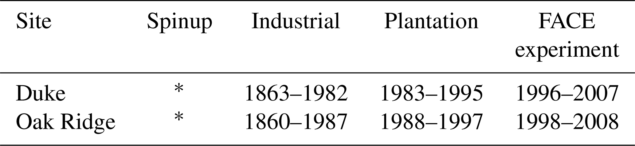
For both sites and both sets of simulation, several simulation steps have been carried out in order to better represent the site and its history. The protocol is the following. First, there is a spinup. We cycled over a spinup forcing that uses meteorological data of the FACE experiment with CO₂ concentration held constant at pre-industrial level. The criterion to end the spinup is discussed in the next section. Then, CO₂ concentration was gradually increased to simulate the industrial period. Historical meteorological forcing was used. This step lasted until the start of the forest plantation. At both sites, a clearing occurred before tree planting. Therefore, the biomass was reset to 0 and a simulation was run until the beginning of the FACE experiment. This step is referred to as plantation. There were 2 simulations run for the FACE experiment: one at ambient CO₂ and one at elevated CO₂. Table 3 summarizes the simulation protocol at each site.

Table 3 Simulation steps carried out to equilibrate the model and to represent the sites history. For the spinup duration ^*, see Table 4.

3.3 Spinup

The spinup is a critical part of the simulation process and there can be several criteria to define whether a simulation is ready to be run. Typically, spinup is considered complete when carbon pools reach a steady state, i.e., when the average total carbon stock per year stabilizes indicating system equilibrium.

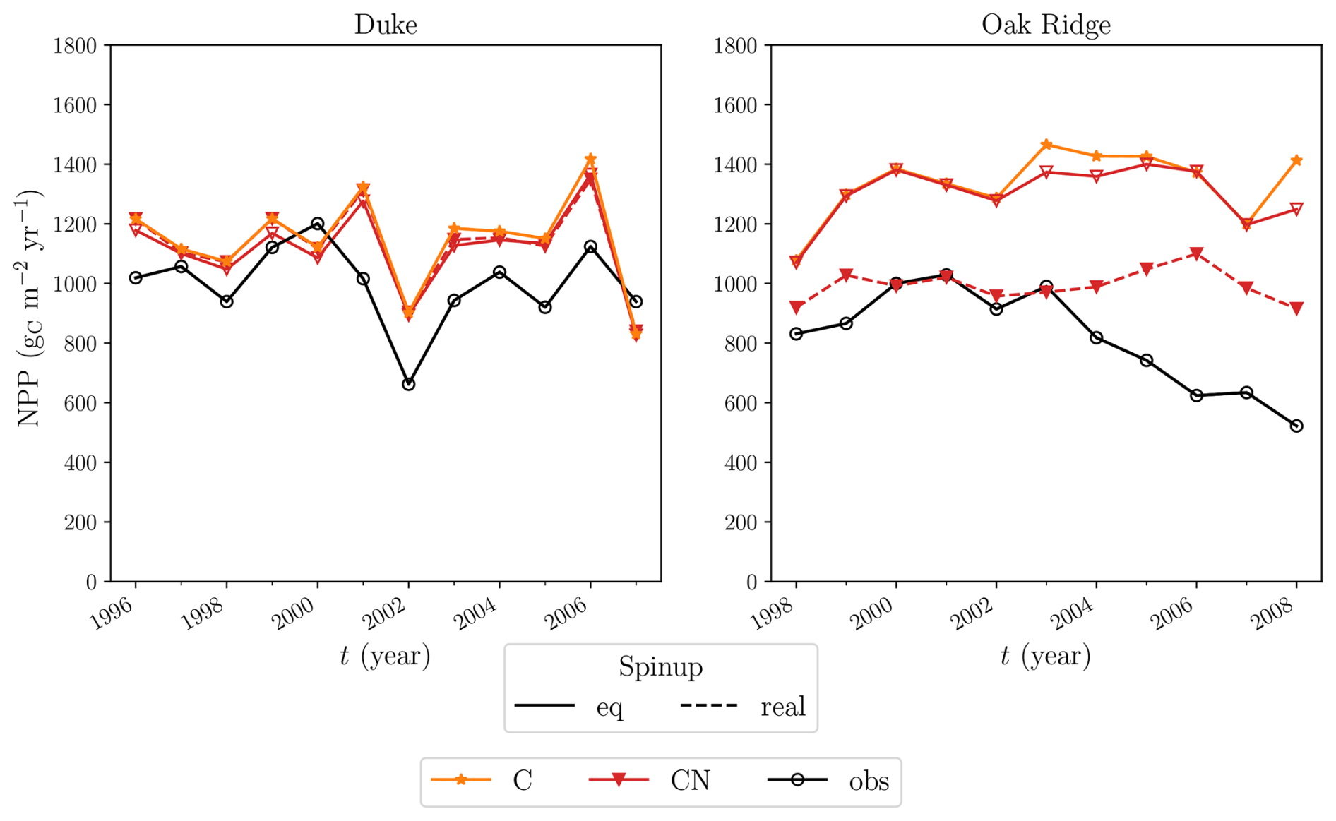
Figure 3 Simulated NPP in g_C m⁻² yr⁻¹ at ambient CO₂, starting from equilibrated (spinup eq, plain lines) and observation-derived soil carbon pools (spinup real, dotted lines) for Duke (left panel) and Oak Ridge (right panel). Results from C (orange stars) and CN (red triangles) simulations are compared to observations extracted from Zaehle et al. (2014) (black circles).

A first spinup was done following this method for both sites. At Duke, equilibrium was reached after 1200 and 2400 years for C and CN version respectively. At Oak Ridge, equilibrium was reached after 1100 and 2200 years. However, this method overestimates soil carbon content compared to field observations. For the top 15 cm of soil, observed values are 1977 g_C m⁻² at Duke (Lichter et al., 2005), and 2670 g_C m⁻² at Oak Ridge (Jastrow et al., 2005). For each set of simulation (C or CN), we compute the total below-ground litter and soil carbon in the first four soil layers to match the measurement depth. Table 4 summarizes the simulated values, which significantly exceed observed levels. However, letting the system reach equilibrium assumes that vegetation and soils at these sites are the result of hundreds of years of present day climate with no disturbances, which is not realistic. In addition, the land use changes are not taken into account. Both sites have an agricultural past: mowed grass at Duke and crops at Oak Ridge (Hamiton et al., 2002; Iversen et al., 2012). Chapter 4 of special report on Climate Change and Land (Intergovernmental Panel On Climate Change, 2022) documents a strong reduction of soil C content in cropland and grasslands compared to forest. This may explain a large part of the discrepancies between the model and the observations.

Table 4 Total soil carbon (soil litter and SOC) in g_C m⁻² in the first soil layers as measured and after equilibrium is reached in simulations. Time in years to match observed values in the “spinup real”.

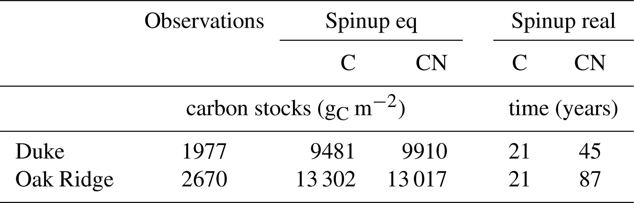
An alternative approach is to stop the spinup once the soil C content reaches observed values. This method resulted in much shorter spinup durations: 21 and 45 years for the C and CN versions respectively, at Duke; and 21 and 87 years at Oak Ridge. The first spinup type is denoted as “eq” (equilibrium-based) and the second “real” (observation-based) in the following sections.

Then from each spinup type, industrial, plantation and FACE experiments simulations are conducted. Figure 3 shows the impact of the spinup on the NPP results. For both sites, the C only simulations are not impacted by the type of spinup. However for the CN simulations, discrepancies are observed due to N limitations. The initial condition defines the N status in the system, a greater C soil content leads to higher mineral N pool which supplies then the labile pool. After the equilibrium spinup, the average N in the system (N_min+N_labile) is of 3.24 g_N m⁻² at Duke and of 5.72 g_N m⁻² at Oak Ridge. For the spinup “real”, we found a value of 1.64 g_N m⁻² at Duke and 3.99 g_N m⁻² at Oak Ridge. Note that the NPP simulated by the CN version after equilibrium spinup is very close to the one simulated by the C version, indicating that the equilibrium spinup results in a system not limited in N. We chose the type of spinup that results in a soil carbon content equal to observations. In what follows, all simulations results originate from a spinup “real”. In this configuration, the system is not at equilibrium. This is closer to the real soil status due to the recent reforestation.

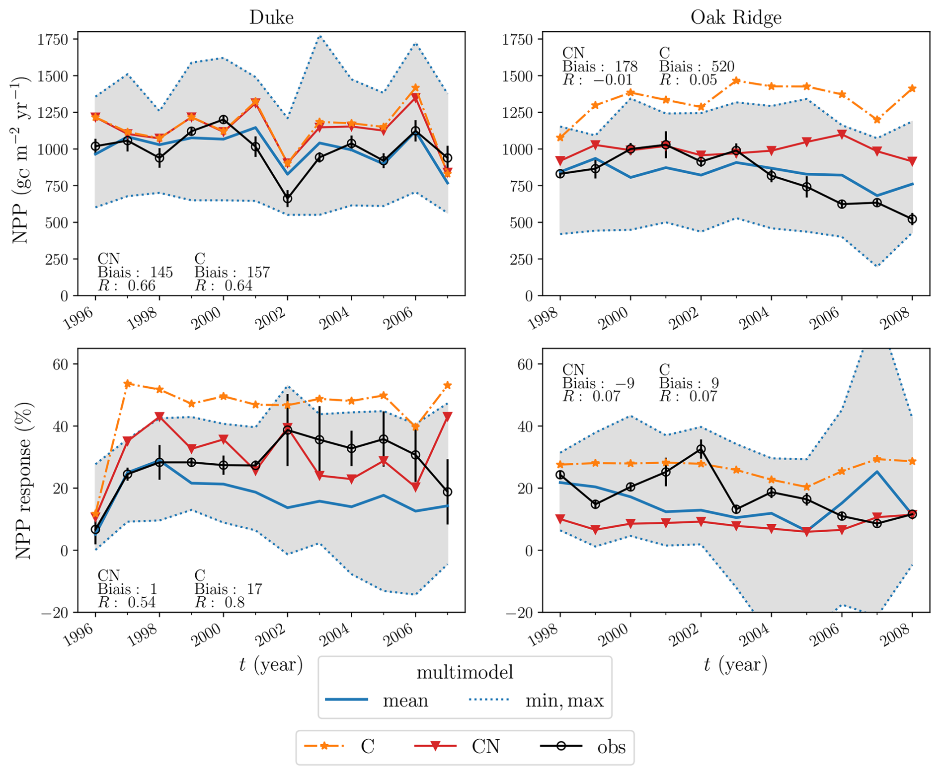
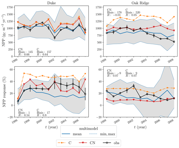
Figure 4 NPP in g_C m⁻² yr⁻¹ on control plots (top panels) and response of NPP to elevated CO₂ in % (bottom panels). Results at Duke (left panels), Oak Ridge (right panels). Comparison of ISBA performance (C version, orange stars, and CN version, red triangles) with multi model analysis conducted by Zaehle et al. (2014) (mean blue thick line, model range: grey area delimited by dotted blue lines) and observations (black circles).

4 Results

4.1 Sensitivity of carbon and nitrogen fluxes to increased CO₂

We evaluate our model by comparing it to observations and multi-model simulations from Zaehle et al. (2014) who evaluated 11 models at the Duke and Oak Ridge sites. We compare our model results with the minimum, maximum and mean of these 11 models, as well as to the observational data given by Zaehle et al. (2014) (Figs 2 and 3). Results are shown on Figs. 4 and 5.

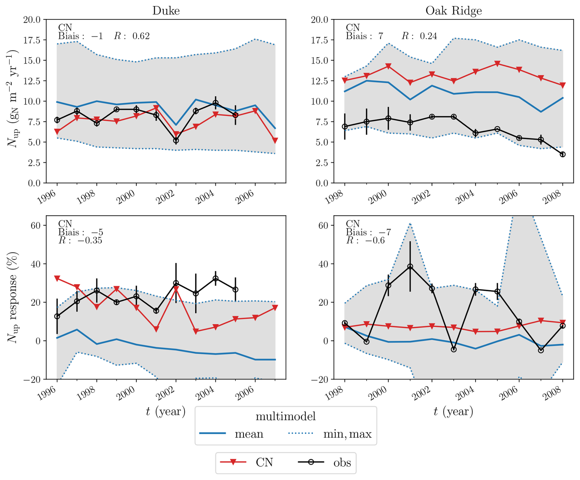
Figure 5 N_up in g_N m⁻² yr⁻¹ on control plots (top panels) and response of N_up in % to elevated CO₂ (bottom panels). Comparison of ISBA performance (CN version, red triangles) with multi model analysis conducted by Zaehle et al. (2014) (mean blue thick line, model range: grey area delimited by dotted blue lines) and observations (black circles).

At Duke under ambient CO₂ (Fig. 4, top left panel), both model versions result in annual NPPs within the 11-model range. The CN version performs better, with a smaller bias relative to observations (145 g_C m⁻² yr⁻¹ vs. 157 g_C m⁻² yr⁻¹ for the C version) and improved interannual variability (correlation of 0.66 vs. 0.64). At Oak Ridge, the C version overestimates NPP (bias of 520 g_C m⁻² yr⁻¹). Results of the CN version are within the 11-model range and better match observations (bias of 178 g_C m⁻² yr⁻¹). However, both model versions fail to capture the observed post-2003 decline in forest productivity associated with progressive nitrogen limitation (Norby et al., 2010), resulting in weak correlations with observations. This could be explained by an overestimation of the initial inorganic N stocks as discussed by Zaehle et al. (2014). At elevated CO₂, the C-only version overestimates the NPP response at both sites (Fig. 4, bottom panels). Including N limitation (CN version) reduces this response. It is in better agreement with the observations at Duke (smaller bias), but the N limitation at Oak Ridge is excessive (strong negative bias). At Duke, the C version of the model accurately represents the inter-annual variability of the response, as indicated by a high correlation. The correlation decreases with the CN version. At Oak Ridge, both versions of the model yields weak correlation.

Figure 5 shows the annual N assimilation flux from soil to plant, N_up, which can only be analyzed with the CN version of the model. Under ambient CO₂ (top panel) N_up is slightly underestimated at Duke (bias of −1 g_N m⁻² yr⁻¹) and overestimated at Oak Ridge (bias of 7). At both sites, the model shows weak skill in reproducing the interannual variability. At Duke, the modeled CO₂ response is in good agreement with the observations and performs better than the multi-model mean. At Oak Ridge, the CO₂ response of the uptake flux is close to the multi-model mean but both fail to represent the inter annual variability. On average, an increase of the uptake flux due to elevated CO₂ is observed and modeled at Duke and Oak Ridge to sustain the increase in NPP. However, the underlying process differ between sites. At Duke, SOM decomposition happened faster, increasing mineralization and thus available N (Drake et al., 2011). At Oak Ridge, increased C allocation to fine roots led to greater root biomass and deeper roots allowing trees to access more N. This adaptive response is likely linked to the site history, a former agricultural land (Iversen et al., 2012). Such adaptation strategies are not represented by the model. Instead, in the model, the increased N_up is due to increased available N in the mineral pool related to increased BNF mostly. Processes linked to the soil N dynamics are discussed in Sect. 4.3.

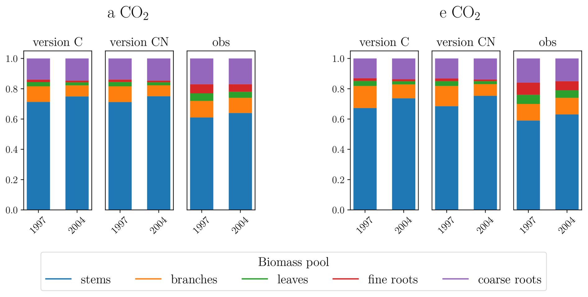
Figure 6 Partitioning of carbon in the biomass pools as a function of time at Duke. Comparison between the C (left column panels) and CN (middle column panels model versions, and the observations (McCarthy et al., 2010) (right column panels), for plots under ambient (left panels) and elevated CO₂ (right panels).

4.2 Vegetation and soil carbon stocks and response to CO₂

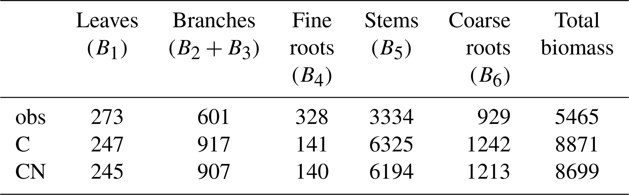
At Duke, under ambient CO₂, the C version overestimates biomass in the woody components for the year 1997 (Table 5). This leads to an overestimation of the total biomass, although it underestimates fine-root biomass. Including the nitrogen cycle slightly reduces woody biomass but does not improve leaves and fine-root biomass. At Oak Ridge, the total biomass simulated for 1998 is 7097 g_C m⁻² using the C version and 5755 g_C m⁻² using the CN version. As at Duke, inclusion of the N cycle reduces C accumulation in woody biomass. No observational data are available for comparison.

Table 5 Observed biomass (McCarthy et al., 2010) vs. simulated (versions C and CN) in g_C m⁻² for the year 1997 on ambient plots at Duke.

At Duke under ambient CO₂, the carbon partitioning between biomass pools changed over time (Fig. 6) as discussed in McCarthy et al. (2010). The allocation to woody tissues increased, which is expected in an ageing forest. Both model versions reproduce this behavior, although the magnitude of the increase is smaller, and carbon allocation to wood is overestimated.

At Oak Ridge, no allocation shift was observed during the first 3 years, as indicated by biomass increments measured in 1998, 1999 and 2000 (Table 6). The proportion of C allocated to wood ($\mathrm{\Delta }(B_{\mathrm{2}}+B_{\mathrm{3}}+B_{\mathrm{5}})/\mathrm{\Delta }{B}_{\mathrm{tot}}$) and fine roots ($\mathrm{\Delta }{B}_{\mathrm{4}}/\mathrm{\Delta }{B}_{\mathrm{tot}}$) remained constant over time. On average, 60 % of the carbon increment was stocked in wood and 12 % in fine roots. Both model versions similarly show no allocation shift during the first 3 years or over the full simulation period (1998–2008). However, the modeled proportion of carbon increments allocated to wood is higher than observed (84 % in average) while it is underestimated for fine roots (−1 % in average). Inclusion of the nitrogen cycle does not affect the partitioning of carbon in the biomass, neither its evolution during the three years.

Table 6 Increase of fine roots ΔB₄, wood $\mathrm{\Delta }(B_{\mathrm{2}}+B_{\mathrm{3}}+B_{\mathrm{5}})$, and total biomass ΔB_tot for years 1998, 1999 and 2000 at Oak Ridge in g_C m⁻² yr⁻¹. Observations extracted from Norby et al. (2002) are compared to simulations (C and the CN versions).

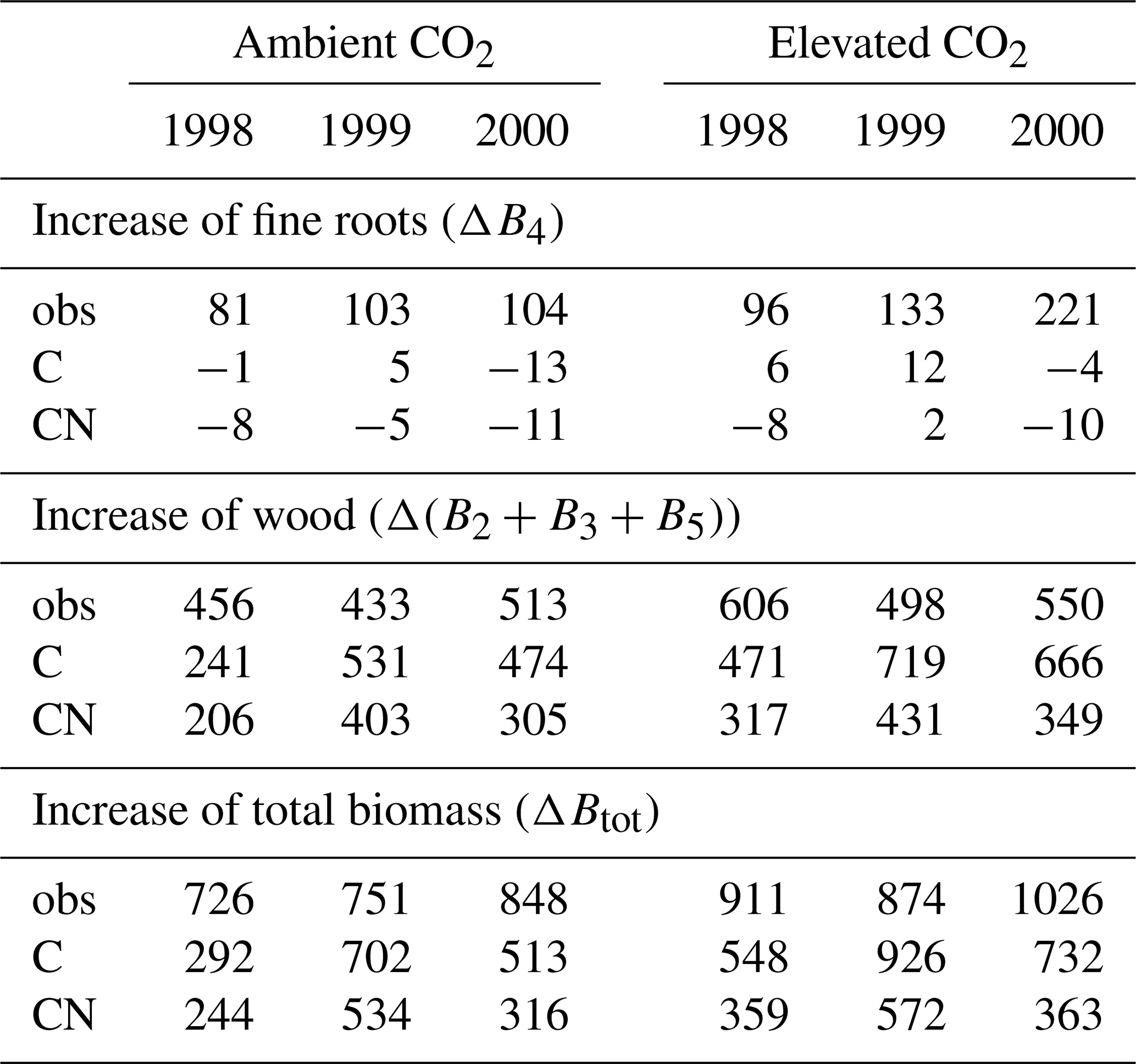
Under elevated CO₂ treatment, total biomass at Duke increased by 6204 g_C m⁻² between 1997 and 2004 (McCarthy et al., 2010), corresponding to a 34 % relative to ambient plots. During the same time period, the C version simulates a 74 % increase in response to elevated CO₂, whereas the CN version a 47 % increase. At Oak Ridge, between 1998 and 2008, we find a 37 % increase according to the C version and 15 % for the CN version. No data are available for comparison. Overall, the CN version limits the modeled carbon sink, which is an improvement at the Duke site. CO₂ enrichment has no effect on the partitioning of carbon in biomass at Duke (Fig. 6), a feature that is well represented by both model versions. As mentioned earlier, an increase in fine root biomass was observed at Oak Ridge (Norby et al., 2002), from 11 % in 1998 to 22 % in 2000 (Table 6). Both model versions fail to represent this shift as the model does not include a dynamic allocation scheme. The N cycle does not have an impact on the partitioning of biomass.

Soil carbon content observations are only available for the upper layers of the soil. Table 7 summarizes SOC content in the soil between 0 and 15 cm measured at Duke and Oak Ridge together with simulation results. Both the model versions overestimate the SOC content, but the addition of the nitrogen cycle improves the results.

Table 7 Simulated vs. observed carbon content in soil between 0 and 15 cm in 2002 in g_C m⁻². Simulations are from C and CN versions. C content is computed as the sum of soil litter C and SOC on the first 4 layers. Observations data are extracted from Lichter et al. (2005) for Duke and Jastrow et al. (2005) for Oak Ridge.

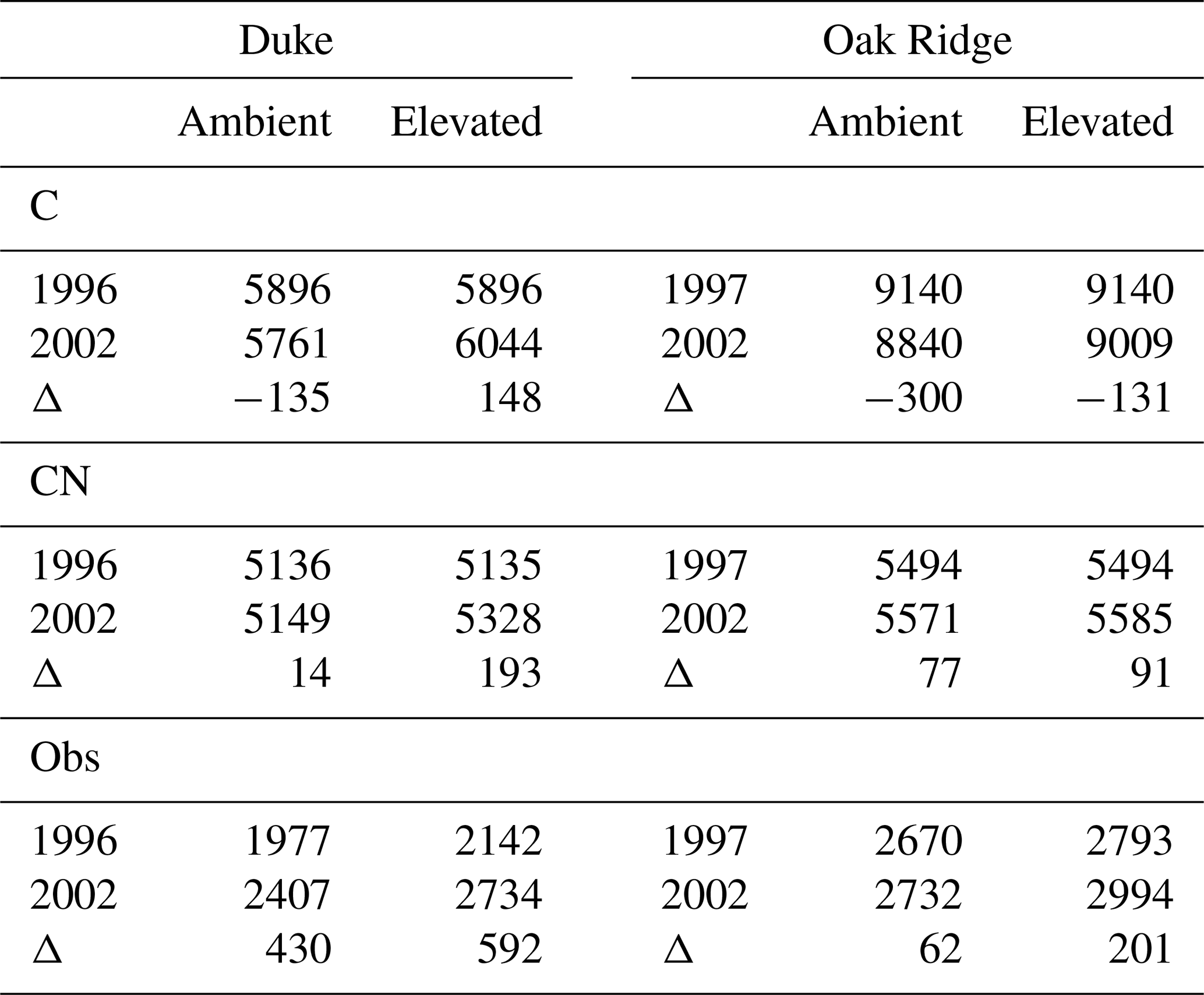
In response to elevated CO₂, contrasting dynamics were observed at Duke and Oak Ridge. At Duke, the forest floor mass (litter and fine roots) increased under elevated CO₂, but little SOM accumulation was observed (Drake et al., 2011). Conversely, at Oak Ridge, there was no accumulation in the forest floor (Johnson et al., 2004), while SOM accumulation occurred due to increased fine root production rapidly decomposed (Iversen et al., 2012) (see Table 7, accumulation of C in the first soil layers is 3 times higher at elevated CO₂). These contrasting dynamics in SOC and forest floor are not well represented by the model. There is an increase in SOC content modeled in response to elevated CO₂ at both sites. This accumulation is stronger at Duke than at Oak Ridge. The C version models an increase in SOC accumulation of 210 % at Duke and 56 % at Oak Ridge while the CN version results in 1279 % increase at Duke and 18 % at Oak Ridge. Both model versions simulate an increase of C in the forest floor (computed as surface litter L_surf and fine-roots B₄) in response to elevated CO₂ at both sites. The increase is smaller with the CN version.

This study points out the limitations of the carbon cycle model in ISBA. The allocation pattern is not flexible, therefore adaptions to environmental changes cannot be captured. This impacts carbon partitioning within the soil and the representation of decomposition processes. Vertical soil discretization is important to improve the modeling of C and N dynamics (Norby et al., 2010; Iversen et al., 2012; Zaehle et al., 2014). However this is not sufficient to represent the response to elevated CO₂ as shown here. Other processes are lacking such as a dynamical root profile or the effect of microbial communities (Drake et al., 2011).

4.3 Modeled N dynamics

This section focuses on the CN version of the model to evaluate the new implementation. Figure 7 shows the dynamics of nitrogen in the vegetation and Fig. 8 its dynamics as bulk in the soil. The vegetation labile pool and the soil mineral pool are coupled through the uptake flux (shown in Fig. 8) that determines N availability for plant growth. In early spring, photosynthesis is mainly sustained by the labile pool. Progressively, when the labile pool empties around April or May, the N $/$ C ratio of leaves starts to decrease. This triggers an increase in uptake flux that is able to sustain NPP through the summer. Figure 7 shows that the N $/$ C ratio evolves as a function of the nitrogen demand. The ratio decreases as the labile pool is depleted. There is no observation to compare these results with, but the model behaves as expected.

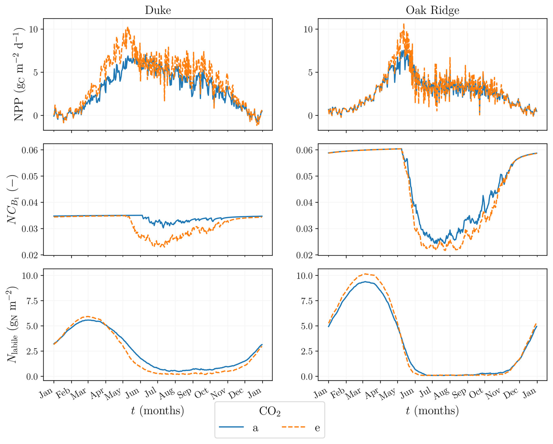
Figure 7 Average seasonal cycle of NPP, $N{C}_{B_{\mathrm{1}}}$, and N_labile at Duke (left panels) and Oak ridge (right panels) with the CN model version at ambient CO₂ (blue plain lines) and elevated CO₂ (orange dashed lines).

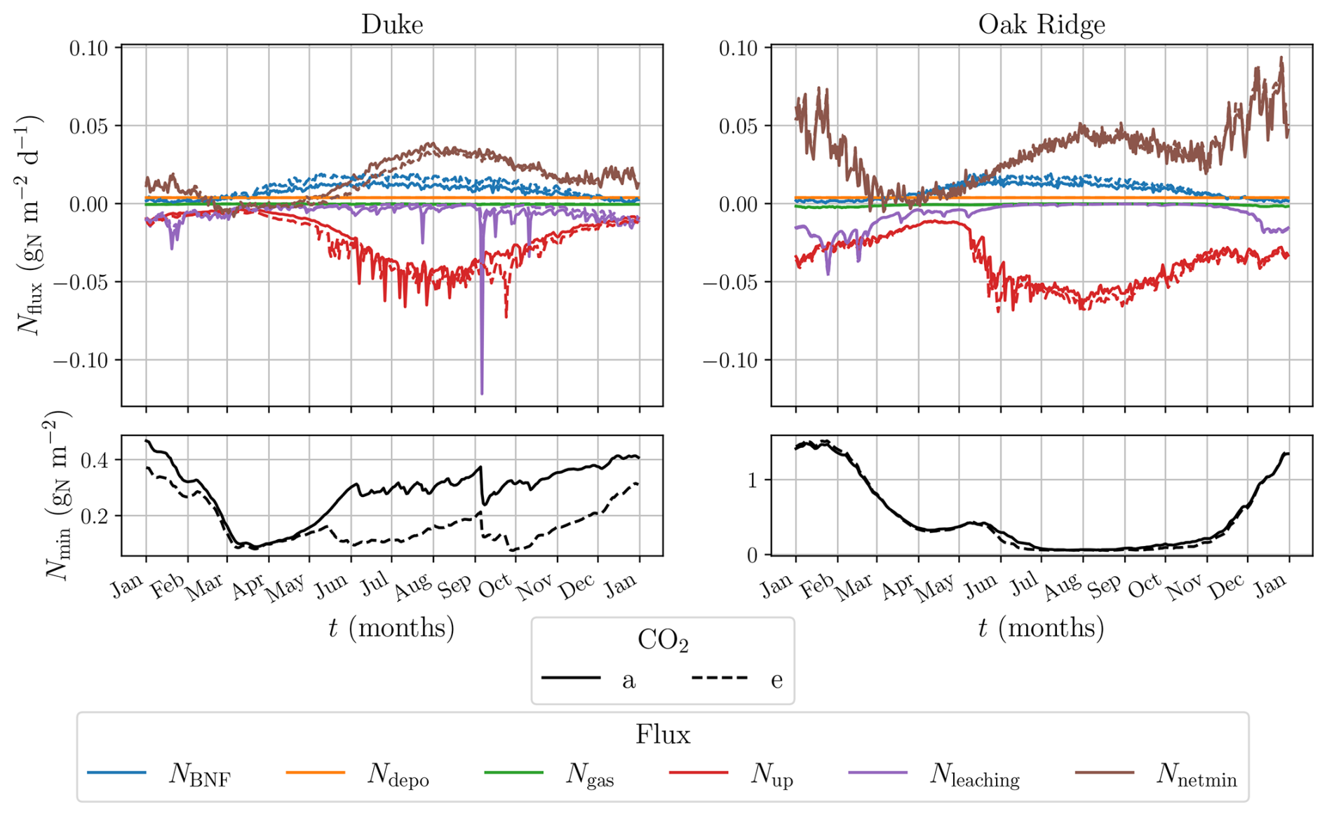
Figure 8 Average seasonal cycle of the simulated bulk mineral N pool (bottom panels) and its input and output fluxes (top panels), at Duke (left panels) and Oak Ridge (right panels), at ambient (plain line) and elevated CO₂ (dashed line). Input fluxes are positive and are the following: biological fixation N_BNF, deposition N_depo, and net mineralization N_netmin. Output fluxes are negative and are the following: gas losses N_gas, plant uptake N_up and leaching N_leaching. Pool content is shown in g_N m⁻² and fluxes are in g_N m⁻² d⁻¹.

The main source of mineral N at Duke and at Oak Ridge is net mineralization. BNF is of the same order of magnitude at both sites (see Table 8), which is consistent with the similar magnitude of NPP at the two sites, as BNF is proportional to NPP. A new global BNF estimate suggests that the BNF rate used in this study overestimates this flux (Reis Ely et al., 2025). They evaluate a BNF flux of 0.35 g_N m⁻² yr⁻¹ for evergreen needleleaf forests such as Duke and of 0.61 g_N m⁻² yr⁻¹ for deciduous broadleaf forests such as Oak Ridge. As N_BNF varies with NPP, it peaks in summer. N_depo is prescribed and identical at both sites. Net mineralization however is twice as high at Oak Ridge as at Duke, especially in winter. As a result, the mineral N pool is larger at Oak Ridge for most of the year. This drives soil N dynamics, as all output fluxes are proportional to N_min. N_leaching, N_gas, and N_up are hence greater at Oak Ridge.

Table 8 Annual input and output fluxes that contribute to the mineral nitrogen dynamics. Fluxes are in g_N m⁻² yr⁻¹.

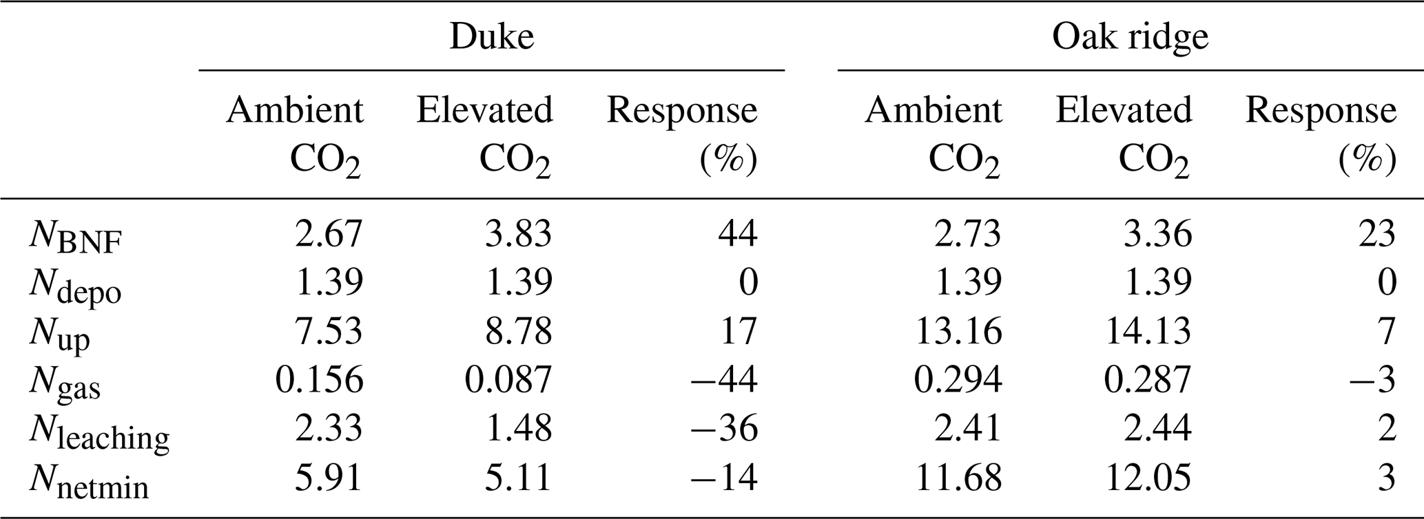
Few measurements are available for comparison. At Duke, Johnson et al. (2004) measured in 1998 on ambient plots an annual N₂O flux of 0.0070 g_N m⁻² yr⁻¹, and an annual leaching flux < 0.001 g_N m⁻² yr⁻¹. For the same year, the model simulates an N₂O flux that is twice as high (0.0162 g_N m⁻² yr⁻¹) and overestimates by several orders of magnitude the leaching flux (3.39 g_N m⁻² yr⁻¹). Reasons for this higher leaching are related to the vertical profile of the soil discussed further down. Calibration of the gaseous outputs is difficult due to the limited number of observations available at these sites. A multi-site analysis carried out by Ma et al. (2022) provides estimates of the N₂O fluxes. In temperate evergreen coniferous forests, the average flux is of 0.0568 g_N m⁻² yr⁻¹. As a comparison, the model yields on average at Duke on ambient plots 0.0142 g_N m⁻² yr⁻¹. For temperate deciduous forests, the observed value is 0.0470 g_N m⁻² yr⁻¹ and at Oak Ridge the average flux on the ambient plots is 0.0267 g_N m⁻² yr⁻¹. Gas losses will be studied in the future on agricultural surfaces where more N₂O data are available.

To better understand the dynamics of the net mineralization flux, Fig. 9 depicts the mineralization and immobilization fluxes. Mineralization due to respiration of SOC pools, F_SOC, dominates the net mineralization flux at both sites (purple line). The mean annual amount of carbon decomposition is higher at Duke than Oak Ridge, as indicated by heterotrophic respiration rates of 357 g_C m⁻² yr⁻¹ at Duke and 324 g_C m⁻² yr⁻¹ at Oak Ridge. This results in higher F_SOC at Duke. Inputs from surface biomass, $F_{B_x,L_{\mathrm{surf}}}$ result from the balance between the N $/$ C ratio of biomass and that of surface litter. This balance is controlled by the N $/$ C ratio of leaves, the only one flexible in the model. Therefore $F_{B_x,L_{\mathrm{surf}}}$ is greater during winter, when nitrogen demand is low and leaf N $/$ C ratio is high. This leads to an accumulation of nitrogen near the soil surface as exhibited by Figs. A2 and A3. $F_{B_x,L_{\mathrm{surf}}}$ and, to a lesser extent, $F_{B_x,L_{\mathrm{soil}}}$, are greater at Oak Ridge because the imposed N $/$ C ratios of biomass pools in broadleaf deciduous trees are higher than those of needleleaf evergreen trees (Table B1). Although annual biomass turnover is greater at Duke (688 g_C m⁻² yr⁻¹) than at Oak Ridge (615 g_C m⁻² yr⁻¹), the higher N $/$ C ratios of biomass pools at Oak Ridge result in greater N release at that site. Around March at Duke, net mineralization is dominated by immobilization associated with surface litter decomposition that depletes the mineral pool (Fig. A2). The immobilization flux from litter decomposition is stronger at Duke, again due to the lower N $/$ C ratios.

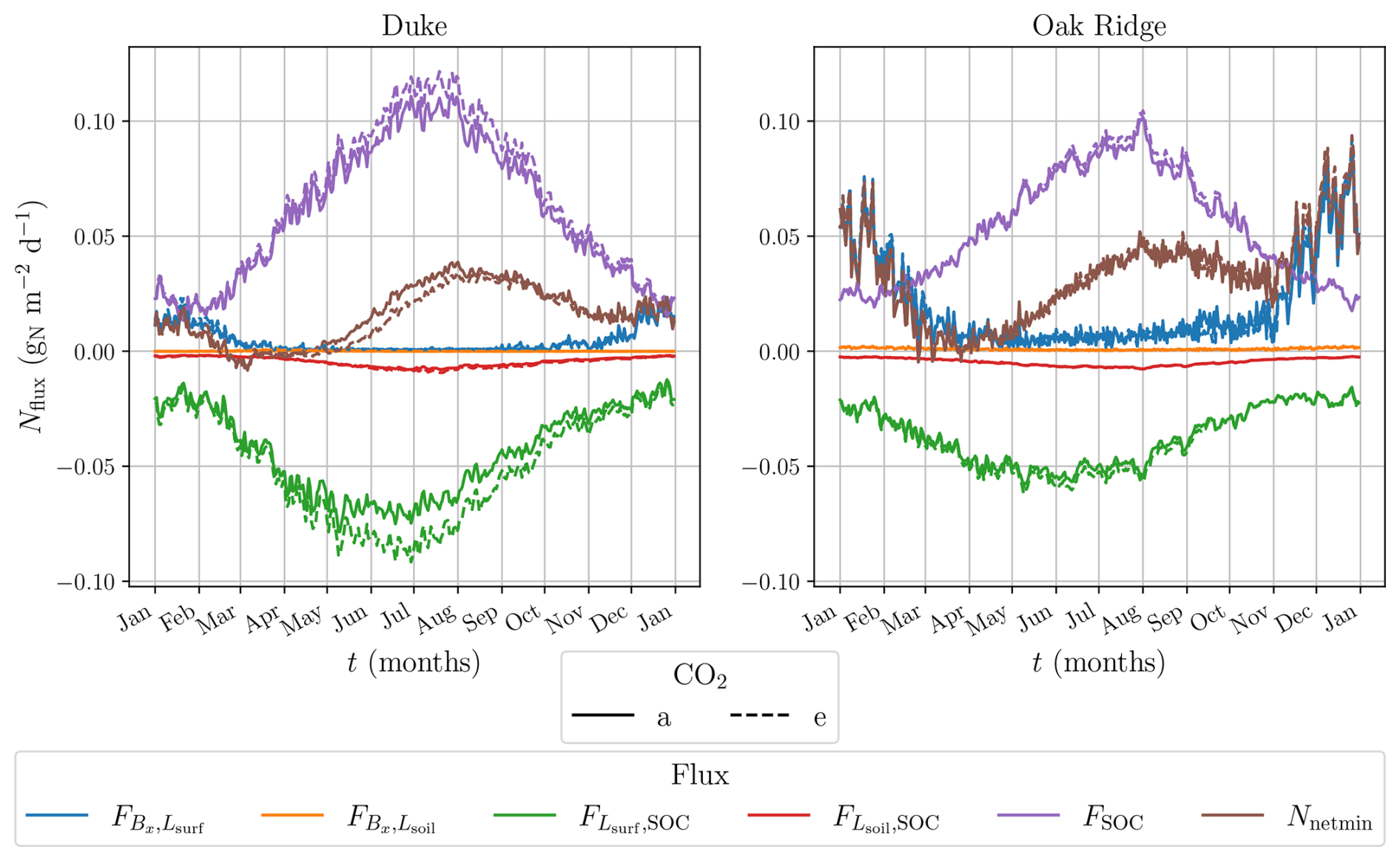
Figure 9 Climatology of the simulated mineralization and immobilization fluxes as well as the net mineralization flux. $F_{B_x,L_{\mathrm{surf}}}$ and $F_{B_x,L_{\mathrm{soil}}}$ are N inputs from biomass turnover to surface litter and soil litter, respectively. $F_{L_{\mathrm{surf},\mathrm{SOC}}}$ and $F_{L_{\mathrm{soil},\mathrm{SOC}}}$ are immobilization fluxes from surface litter and soil litter decomposition to SOC pools, respectively. F_SOC is the mineralization flux from SOC pools decomposition. Fluxes are in g_N m⁻² d⁻¹. Results for Duke are on the right panel and for Oak ridge on the left. Results are shows for plots at ambient and elevated CO₂.

As mentioned in Sect. 2.6, the current version of the model does not represent the vertical movement of N in the soil. Therefore, to avoid unrealistic accumulation of N, we imposed a vertical profile of some input and output fluxes along the soil depth. N resulting from N deposition for instance would otherwise accumulate in the upper layer of the soil. Both N_BNF and N_depo are distributed according to the soil water profile (Eq. 12 and Fig. A1). Therefore, deeper soil layers are more enriched in N because they contain more water (Figs. A2 and A3). This is a model artifact that will be addressed in a future version of the model through an explicit representation of vertical nitrogen transport in the soil. The imposed vertical profiles of gas loss and leaching follow the vertical profile of mineral N in the soil. N uptake follows the root profile and is proportional to mineral N. Because net mineralization provides a high supply of N near the soil surface, uptake fluxe is greatest in the upper soil layers.

In response to elevated CO₂, the BNF which is strongly tied to the NPP, is enhanced on both sites. At Duke, the increase of litter enhances the immobilization flux, thereby reducing net mineralization, whereas at Oak Ridge, there is little change in net mineralization. This is not coherent with observations: the increase in forest floor at Duke stimulated microbial activity, accelerating SOM decomposition and mineralization, thereby increasing N availability (Drake et al., 2011). At Oak Ridge, it is the increase in fine roots that increased the SOC content due to fast root turnover, leading to higher immobilization and reduced N availability (Iversen et al., 2012). These discrepancies originate from differences in the simulated soil carbon dynamics. Moreover, measurements show that N $/$ C ratios are important parameters that control the net mineralization flux. Plants can adapt to N shortage by decreasing their N $/$ C ratio. This dampens N-limitation effects but affects the litter quality: immobilization is increased resulting in less N available (Finzi et al., 2006). However implementing flexible N $/$ C ratios in models is not straightforward as identified by Zaehle et al. (2014) multi model analysis. Without appropriate constraints, such flexibility can lead to unrealistic stoichiometric ratios (Zaehle et al., 2014).

In the simulations, the main source of new N is the BNF, proportional to NPP that increases under elevated CO₂ conditions. The newly available N is used by plants (increase of N_up). BNF is an important external source of nitrogen and can alleviate the N limitation (Liang et al., 2016). However, external nitrogen inputs (mostly ammonia) are known to directly regulate BNF activity in cells (Dixon and Kahn, 2004), as well as in diverse soil and forest organism (e.g., Ackermann et al., 2012 in moss soil carpet, Darnajoux et al., 2022 in coastal sediment). The current parametrization does not take into account the N status of the soil. We have implemented a straightforward BNF parametrization as it has been done in other land surface models. However, some works are critical about the pertinence of using NPP to model BNF and its validity is questioned (Wieder et al., 2015b; Hupperts et al., 2021; Davies-Barnard et al., 2020). In particular, for future predictions, the NPP dependent parametrization is sensitive to CO₂ increase and is probably not realistic (Thomas et al., 2015; Reis Ely et al., 2025). Following the work of Kou-Giesbrecht and Arora (2022), next steps will be dedicated to implement a more process-based parametrization of BNF. First, it is important to differentiate symbiotic from asymbiotic BNF as it does not involve the same processes (Meyerholt et al., 2016; Hupperts et al., 2021; Kou-Giesbrecht et al., 2025). On one hand, symbiotic BNF is directly linked to plant needs and is another direct N source in addition to the root N uptake. A resource optimization framework such as proposed by Rastetter et al. (2001) integrates the C cost of each process and improves the model response to elevated CO₂ and increase in N deposition (Meyerholt et al., 2016; Fisher et al., 2010; Kou-Giesbrecht and Arora, 2022). On the other hand, free living BNF plays a crucial role in providing mineral N needed for specific environmental functionalities such as litter decomposition. This pathway dominates some ecosystems where N fixer species are scarce (Reed et al., 2011). Moreover, both symbiotic and asymbiotic processes are temperature dependent but with contrasting optimums. Due to the predicted rising temperature, this is an important aspect to consider (Kou-Giesbrecht and Arora, 2022; Yuan et al., 2025).

5 Conclusions

In this study, we document the development of the nitrogen cycle in ISBA, the land surface component of the CNRM ESM. The model is evaluated at two FACE experiment sites: Duke and Oak Ridge. We compare the performance of the C (reference version) with that of the CN version that uses the newly implemented N cycle.

Comparison with the multi-model analysis carried out by Zaehle et al. (2014) shows that the CN version reduces several biases present in the C version of the model. Simulations performed with the new version are in the multi-model range, and the response to elevated CO₂ is closer to observations.

The C version of ISBA overestimates the carbon stocks at both sites. The new implementation improves the results, as nitrogen limitations constrain photosynthesis, resulting in less carbon entering the system. All carbon pools are reduced when the nitrogen cycle is added. Although the model does not capture site-specific adaptative responses, such as allocation shifts or microbial activity, it does accurately depict the main features of the response to elevated CO₂. Carbon storage increases under elevated CO₂, but this carbon sink is substantially reduced when nitrogen cycle processes are taken into account.

The N dynamics reproduce the main expected features. However, biases from the C dynamics of ISBA are propagated to the coupled C–N dynamics. This could be addressed by implementing flexible N $/$ C ratios, constraints on the allocation patterns or an evolving root profile. While the model does not capture site-specific adaptative strategies, its overall performance is encouraging. Further improvements could include an explicit representation of vertical mineral nitrogen dynamics and a more process-based parameterization of BNF.

Appendix A: Carbon dynamics

ISBA represents the vegetation by six biomass pools:

• B₁, leaves

• B₂, a structural pool representing stems in the case of grass and crop, and new twigs for trees

• B₃ for numerical stability

• B₄ fine roots and root sapwood

• B₅ aboveground woody biomass (trunk and branches)

• B₆ belowground woody biomass (root heartwood).

Herbaceous plants are described by the 4 first pools while trees by the 6 biomass pools. The assimilated carbon is first allocated to the leaves. It is then reallocated to the other biomass pools using different empirical allometric relations (Gibelin et al., 2008). The dynamics of the biomass pools is described by the following equation:

$$\begin{array}{}\text{(A1)}& \begin{array}{rl}{\displaystyle \frac{\mathrm{d}{B}_x}{\mathrm{d}t}}=& A_x\left(t\right)-M_x\left(t\right)-S_x\left(t\right)-R_x\left(t\right),\\ & x\in \mathit{\{}\mathrm{1},\mathrm{2},\mathrm{3},\mathrm{4},\mathrm{5},\mathrm{6}\mathit{\}}\end{array}\end{array}$$

where A_x is the incoming flux of carbon, M_x the mortality computed as a turnover, S_x the carbon that is transferred to the other pools and R_x the respiration. For leaf biomass (B₁), A₁ is the carbon assimilated by photosynthesis. For the 5 other pools, A_x is the C reallocated from the other pools (S_y≠x). Mortality and storage are computed from a decline term D_x:

$$\begin{array}{}\text{(A2)}& D_x=B_x\left(\mathrm{1}-\exp \left({\displaystyle \frac{\mathrm{\Delta }t}{{\mathit{\tau }}_x}}\right)\right)\end{array}$$

where τ_x is a characteristic time depending of the pool. This quantity is then divided into mortality and storage. Biomass dynamics is computed once a day.

The litter and soil carbon dynamics follow the CENTURY model (Parton et al., 1988). There are two aboveground litter pools: a structural, C₁ and a metabolic C₂. The dynamics is described by:

$$\begin{array}{}\text{(A3)}& {\displaystyle \frac{\partial C_i}{\partial t}}=T_i+\sum _{j\ne i}\left(\mathrm{1}-r_j\right)f_{ij}{F}_{\mathrm{oxic}}^j-F_{\mathrm{oxic}}^i,(i,j)\in [\mathrm{1},\mathrm{2}].\end{array}$$

In the soil, the dynamics is modified by Morel et al. (2019) to represent anoxic decomposition and methane-related processes. There are for each layer l two belowground litter pools: structural, C₃ and metabolic C₄, and 3 soil organic carbon pools: an active (C₅), a slow (C₆) and a passive (C₇) carbon pool, which differs from their turnover times. The equation is the following:

$$\begin{array}{}\text{(A4)}& \begin{array}{rl}{\displaystyle \frac{\partial C_i\left(z\right)}{\partial t}}& ={\displaystyle \frac{\partial }{\partial z}}\left[D\left(z\right){\displaystyle \frac{\partial C_i\left(z\right)}{\partial z}}\right]+{\displaystyle \frac{\partial A{C}_i\left(z\right)}{\partial z}}+T_i\left(z\right)\\ & +\sum _{j\ne i}\left(\mathrm{1}-r_j\right)f_{ij}{F}_{\mathrm{oxic}}^j\left(z\right)-F_{\mathrm{oxic}}^i\left(z\right)\\ & -r_{\mathrm{MG},i}\left(z\right){\displaystyle \frac{M_{\mathrm{C}}}{M_{{\mathrm{CH}}_{\mathrm{4}}}}},(i,j)\in [\mathrm{3},\mathrm{7}].\end{array}\end{array}$$

$F_{\mathrm{oxic}}^i$ is the quantity of carbon decomposed in the pool i, a fraction r_i of this is lost as respiration. The remaining decomposed carbon, $(\mathrm{1}-r_i)F_{\mathrm{oxic}}^i$, is divided to the other carbon pools j according a fraction f_ij that is a function of the soil composition and lignin content for litter pools. The surface litter and soil carbon dynamics is computed at the model timestep. In both equations, T_i is computed from the mortality of biomass pools as:

$$\begin{array}{}\text{(A5)}& T_i=\left\{\begin{array}{ll}\sum _{x=\mathrm{1},\mathrm{2},\mathrm{3},\mathrm{5}}{M}_x{f}_{x,i},& \mathrm{for}i=\mathrm{1},\mathrm{2}\\ \sum _{x=\mathrm{4},\mathrm{6}}{M}_x{f}_{x,i},& \mathrm{for}i=\mathrm{3},\mathrm{4}\\ \mathrm{0},& \mathrm{for}i=\mathrm{5},\mathrm{6},\mathrm{7}\end{array}\right.\end{array}$$

where f_x,i is the factor to partition turnover in structural and metabolic.

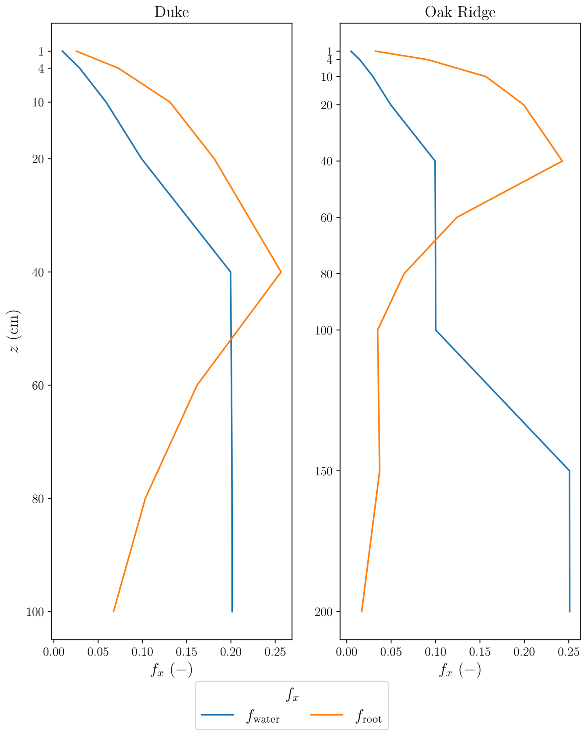
Figure A1 Water profile (blue) and root profile (orange) at Duke (left panel) and at Oak Ridge (right panel). The y axis gives the vertical discretization of the soil, by indicating the depth of each layer.

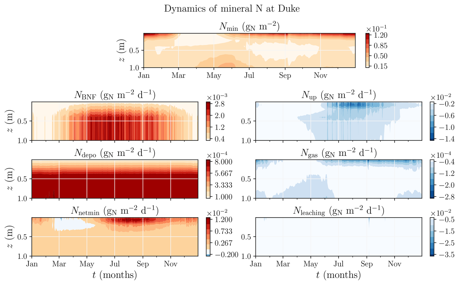
Figure A2 Seasonal cycle of the vertical soil profile of N fluxes and mineral pool at Duke for the reference plot exposed to ambient CO₂ concentration.

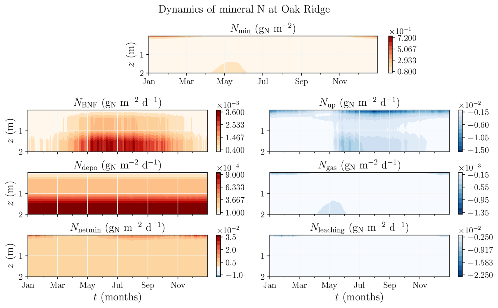
Figure A3 Seasonal cycle of soil profile of N fluxes and mineral pool at Oak Ridge for the reference plot exposed to ambient CO₂ concentration.

Appendix B: N $/$ C ratio

Table B1 N $/$ C stoichiometric ratio in g_N g${}_{\mathrm{C}}^{-\mathrm{1}}$ used in ISBA for the two PFT on which the model is tested: TEmperate Broadleaf Deciduous (TEBD) and TEmperate Needleleaf Evergreen (TENE). Left: N $/$ C ratio for each pool. Right: Maximum and minimum values accepted for the varying N $/$ C stoichiometric ratio of leaves (biomass pool B₁).

Appendix C: Soil nitrogen functions and parameters

C1 Nitrification

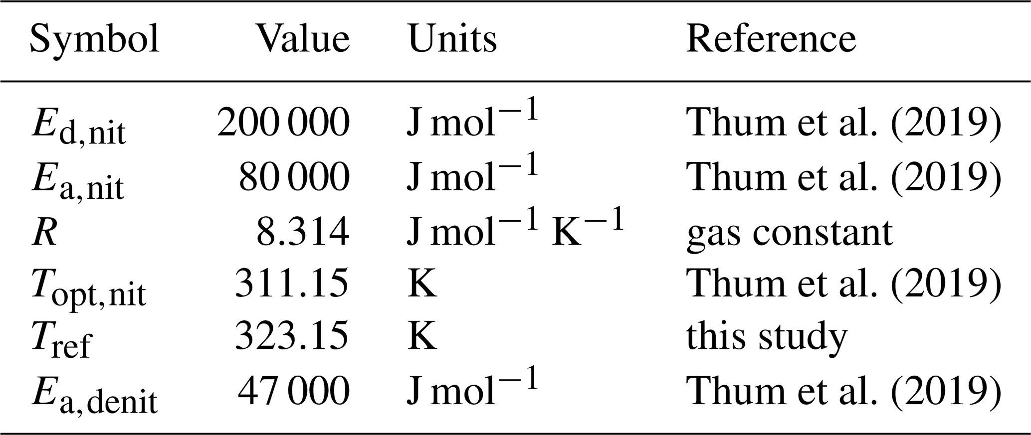
The temperature function for nitrification is described by Eq. (C1) taken from the QUINCY model (Thum et al., 2019). Parameters used in the equation are given in Table C1.

$$\begin{array}{}\text{(C1)}& f\left(T_l\right)=E_{\mathrm{d},\mathrm{nit}}{\displaystyle \frac{\exp \left(\frac{E_{\mathrm{a},\mathrm{nit}}}{R}\frac{T_l-T_{\mathrm{opt},\mathrm{nit}}}{T_l\times T_{\mathrm{opt},\mathrm{nit}}}\right)}{E_{\mathrm{d},\mathrm{nit}}-E_{\mathrm{a},\mathrm{nit}}\times \left(\mathrm{1}-\exp \left(\frac{E_{\mathrm{a},\mathrm{nit}}}{R}\frac{T_l-T_{\mathrm{opt},\mathrm{nit}}}{T_l\times T_{\mathrm{opt},\mathrm{nit}}}\right)\right)}}\end{array}$$

where T_l is the soil temperature in layer l in Kelvin. Nitrification increases as temperature rises. The soil moisture function for nitrification is described by Eq. (C2), which models the moisture dependency with an optimum soil moisture according to Li et al. (2000). There is a moderate effect of moisture but nitrification is slowed if the soil is saturated. Parameters used in the equation are given Table C1.

$$\begin{array}{}\text{(C2)}& f\left({\mathit{\theta }}_l\right)=f_{\max }{\mathit{\theta }}_l^{\mathrm{2}}{\left(\mathrm{1}-{\mathit{\theta }}_l\right)}^{\mathrm{0.5}}\end{array}$$

where ${\mathit{\theta }}_l=\min \left(\mathrm{0},\frac{w_{\mathrm{g},l}-w_{\mathrm{wilt},l}}{w_{\mathrm{sat},l}-w_{\mathrm{wilt},l}}\right)$, w_g,l denotes soil water content in m³ m⁻³, w_sat,l the soil porosity in m³ m⁻³, w_wilt,l the wilting point in m³ m⁻³, and $f_{\max }=\frac{\mathrm{25}\sqrt{\mathrm{5}}}{\mathrm{16}}$ ensures that the function has a maximum value of 1. The parametrization follows experimental observations by Khalil et al. (2004), Ingwersen et al. (1999) and modeling works by Li et al. (1992, 2000), Parton et al. (1996), Xu-Ri and Prentice (2008), Thum et al. (2019), Yang et al. (2009) and Sulman et al. (2019).

Thum et al. (2019)Thum et al. (2019)Thum et al. (2019)Thum et al. (2019)

Table C1 Parameters used to describe nitrification and denitrification.

C2 Denitrification

The temperature function is taken from the QUINCY model (Thum et al., 2019). Denitrification is increasing with temperature as described by:

$$\begin{array}{}\text{(C3)}& f\left(T_l\right)=\exp \left(-{\displaystyle \frac{E_{\mathrm{a},\mathrm{denit}}}{R}}\left({\displaystyle \frac{\mathrm{1}}{T_l}}-{\displaystyle \frac{\mathrm{1}}{T_{\mathrm{ref}}}}\right)\right).\end{array}$$

The parameters are given in the following Table C1.

Appendix D: Nitrogen associated to turnover and decomposition fluxes

D1 Turnover flux from biomass pools to litter pools

The N turnover flux is computed by applying an effective N $/$ C ratio: $N{C}_{\mathrm{eff},B_x}=N{C}_{B_x}\left(\mathrm{1}-f_{\mathrm{trans},x}\right)f_{\mathrm{corr}}$. This takes into account the retranslocation, see Sect. 2.3. The resultant nitrogen flux is obtained by comparing the input flux to what the receiving pool needs. Surface litter is supplied by the turnover of the aboveground biomass pools (1, 2, 3 and 5) and the flux is given by Eq. (D1). Soil litter is supplied by the biomass pools 4 and 6 (root pools), Eq. (D2).

$$\begin{array}{}\text{(D1)}& {\displaystyle }\begin{array}{rl}{F}_{B,L_{\mathrm{surf}}}& =\sum _{x=\mathrm{1},\mathrm{2},\mathrm{3},\mathrm{5}}{f}_{x,\mathrm{1}}{M}_x\left(N{C}_{\mathrm{eff},B_x}-N{C}_{C_{\mathrm{1}}}\right)\\ & +f_{x,\mathrm{2}}{M}_x\left(N{C}_{\mathrm{eff},B_x}-N{C}_{C_{\mathrm{2}}}\right)\end{array}\text{(D2)}& {\displaystyle }\begin{array}{rl}{F}_{B,L_{\mathrm{soil}}}& =\sum _{x=\mathrm{4},\mathrm{6}}{f}_{x,\mathrm{3}}{M}_x\left(N{C}_{\mathrm{eff},B_x}-N{C}_{C_{\mathrm{3}}}\right)\\ & +f_{x,\mathrm{4}}{M}_x\left(N{C}_{\mathrm{eff},B_x}-N{C}_{C_{\mathrm{4}}}\right)\end{array}\end{array}$$

D2 Flux between litter pools and SOC pools

Decomposition from the metabolic aboveground litter pool, denoted $F_{\mathrm{oxic}}^{\mathrm{1}}$, enters the first layer of the active SOC pool (C₅) and releases CO₂ as respiration. Decomposition from the structural surface litter pool, $F_{\mathrm{oxic}}^{\mathrm{2}}$, is divided in a fraction that contains lignin L₂ and goes into the slow SOC pool (C₆), a fraction with no lignin (1−L₂) that flows into the active SOC pool (C₅) and a fraction that goes to respiration.

$$\begin{array}{}\text{(D3)}& \begin{array}{rl}& F_{L_{\mathrm{surf},\mathrm{SOC}}}=L_{\mathrm{2}}\left(N{C}_{C_{\mathrm{2}}}-N{C}_{C_{\mathrm{6}}}\right)F_{\mathrm{oxic}}^{\mathrm{2}}{f}_{\mathrm{2},\mathrm{6}}+\left(\mathrm{1}-L_{\mathrm{2}}\right)\left(N{C}_{C_{\mathrm{2}}}-N{C}_{C_{\mathrm{5}}}\right)F_{\mathrm{oxic}}^{\mathrm{2}}{f}_{\mathrm{2},\mathrm{5}}\\ & +\left(N{C}_{C_{\mathrm{1}}}-N{C}_{C_{\mathrm{5}}}\right)F_{\mathrm{oxic}}^{\mathrm{1}}{f}_{\mathrm{1},\mathrm{5}}\\ & +\underset{\mathrm{respiration}}{\underbrace{\left[\left(\mathrm{1}-L_{\mathrm{2}}\right)\left(\mathrm{1}-f_{\mathrm{2},\mathrm{5}}\right)+L_{\mathrm{2}}\left(\mathrm{1}-f_{\mathrm{2},\mathrm{6}}\right)\right]F_{\mathrm{oxic}}^{\mathrm{2}}N{C}_{C_{\mathrm{2}}}+\left(\mathrm{1}-f_{\mathrm{1},\mathrm{5}}\right)F_{\mathrm{oxic}}^{\mathrm{1}}N{C}_{C_{\mathrm{1}}}}}\end{array}\end{array}$$

The decomposition of the belowground litter follows a similar path. The structural pools C₄ are decomposed into active and slow SOC pools depending on their lignin content (L₄) and the metabolic pools enter the active SOC. The resulting N flux per layer is:

$$\begin{array}{}\text{(D4)}& \begin{array}{rl}& F_{L_{\mathrm{soil},\mathrm{SOC},l}}=L_{\mathrm{4},l}\left(N{C}_{C_{\mathrm{4}}}-N{C}_{C_{\mathrm{6}}}\right)F_{\mathrm{oxic},l}^{\mathrm{4}}{f}_{\mathrm{4},\mathrm{6}}+\left(\mathrm{1}-L_{\mathrm{4},l}\right)\left(N{C}_{C_{\mathrm{4}}}-N{C}_{C_{\mathrm{5}}}\right)F_{\mathrm{oxic},l}^{\mathrm{4}}{f}_{\mathrm{4},\mathrm{5}}\\ & +\left(N{C}_{C_{\mathrm{3}}}-N{C}_{C_{\mathrm{5}}}\right)F_{\mathrm{oxic},l}^{\mathrm{3}}{f}_{\mathrm{3},\mathrm{5}}\\ & +\underset{\mathrm{respiration}}{\underbrace{\left[\left(\mathrm{1}-L_{\mathrm{4},l}\right)\left(\mathrm{1}-f_{\mathrm{4},\mathrm{5}}\right)+L_{\mathrm{4},l}\left(\mathrm{1}-f_{\mathrm{4},\mathrm{6}}\right)\right]F_{\mathrm{oxic},l}^{\mathrm{4}}N{C}_{C_{\mathrm{4}}}+\left(\mathrm{1}-f_{\mathrm{3},\mathrm{5}}\right)F_{\mathrm{oxic},l}^{\mathrm{3}}N{C}_{C_{\mathrm{3}}}}}.\end{array}\end{array}$$

D3 Flux between SOC pools

Decomposition of organic carbon within the active, slow and passive pools results in a N flux of:

$$\begin{array}{}\text{(D5)}& \begin{array}{rl}& F_{\mathrm{SOC},l}=\left(N{C}_{C_{\mathrm{5}}}-N{C}_{C_{\mathrm{6}}}\right)F_{\mathrm{oxic},l}^{\mathrm{5}}{f}_{\mathrm{5},\mathrm{6}}+\left(N{C}_{C_{\mathrm{5}}}-N{C}_{C_{\mathrm{7}}}\right)\\ & F_{\mathrm{oxic},l}^{\mathrm{5}}{f}_{\mathrm{5},\mathrm{7}}+\left(N{C}_{C_{\mathrm{6}}}-N{C}_{C_{\mathrm{5}}}\right)F_{\mathrm{oxic},l}^{\mathrm{6}}{f}_{\mathrm{6},\mathrm{5}}\\ & +\left(N{C}_{C_{\mathrm{6}}}-N{C}_{C_{\mathrm{7}}}\right)F_{\mathrm{oxic},l}^{\mathrm{6}}{f}_{\mathrm{6},\mathrm{7}}+\left(N{C}_{C_{\mathrm{7}}}-N{C}_{C_{\mathrm{5}}}\right)\\ & F_{\mathrm{oxic},l}^{\mathrm{7}}{f}_{\mathrm{7},\mathrm{5}}+\\ & \underset{\mathrm{respiration}}{\underbrace{\left(\mathrm{1}-f_{\mathrm{5},\mathrm{6}}-f_{\mathrm{5},\mathrm{7}}\right)F_{\mathrm{oxic},l}^{\mathrm{5}}N{C}_{C_{\mathrm{5}}}+\left(\mathrm{1}-f_{\mathrm{6},\mathrm{5}}-f_{\mathrm{6},\mathrm{7}}\right)F_{\mathrm{oxic},l}^{\mathrm{6}}N{C}_{C_{\mathrm{6}}}+\left(\mathrm{1}-f_{\mathrm{7},\mathrm{5}}\right)F_{\mathrm{oxic},l}^{\mathrm{7}}N{C}_{C_{\mathrm{7}}}}}.\end{array}\end{array}$$

Appendix E: List of added variables

Table E1 Variables added for the nitrogen cycle.