Optimizing Gaussian process emulation and generalized additive model fitting for rapid, reproducible earth system model analysis

Causes of model uncertainty in complex modeling systems can be identified using large perturbed-parameter ensembles (PPEs), combined with statistical emulators to increase sample size and enable variance-based sensitivity analyses and observational constraint. In global climate models such as the UK Earth System Model (UKESM), these approaches are typically applied at the global or regional mean scales for a limited set of variables. Accelerating progress in understanding the multi-faceted causes of climate model uncertainty, requires implementing such workflows at the model grid box scale, to enable analyses across variables that reveal how uncertainties propagate and interact spatially. However, this approach requires training millions of Gaussian process (GP) emulators and fitting an equal number of generalized additive models (GAMs) – a major computational bottleneck. We present a high-performance, open-source pipeline that introduces optimisations for this workflow. For GP emulation, we implement task-level parallelism and streamlined data handling on high-performance computing systems. For GAM fitting, we integrate a parallelized pyGAM interface with R's mgcv::bam() back end, using fast fREML estimation with discrete smoothing, memory-efficient batching, and improved input–output routines. These changes reduce GP training time by 97.5 % (6177 s → 154 s) and GAM fitting time by 95.2 % (10 623 s → 511 s), yielding a ∼ 25 × faster end-to-end workflow (96 % total runtime reduction) and cutting peak memory use by a factor of 12. Outputs are numerically identical to the baseline implementation (Pearson correlation = 1.00 for both GP and GAM predictions). We demonstrate the approach using a UKESM PPE comprising 221 members scaled up to 1 million using GP emulators, and GAM fits applied to output for a single target variable, to show that the improved performance enables multi-variable, higher-resolution, and potentially multi-model analyses that were previously impractical. These improvements pave the way for PPE studies to scale in scope without compromising statistical fidelity, enabling more comprehensive exploration of model parameter uncertainty within feasible HPC budgets.

1 Introduction

Perturbed-parameter ensemble (PPE) studies are increasingly recognised as a vital tool in climate and Earth system modelling because they provide information needed to characterise model uncertainty and identify its causes. Well designed PPEs enable systematic identification of structural model deficiencies, guide targeted model developments, and provide a basis for rigorous statistical calibration against observations (Carslaw et al., 2026), unlike multi-model ensembles (Stouffer et al., 2017; Durack et al., 2025), which conflate structural and parametric uncertainties in uncontrolled ways. Community assessments consistently argue that PPEs should be prioritised alongside increases in model complexity and resolution, as they offer one of the best opportunities to improve model reliability and provide robust uncertainty quantification for downstream impacts and decision making (Knutti, 2008; Carslaw et al., 2026).

Complex Earth system models are computationally expensive, which typically limits PPEs to hundreds of members. To enable robust statistical analysis of parameter sensitivities and uncertainty, these ensembles are often augmented using model emulation, allowing exploration of millions of parameter combinations at relatively low computational cost (Sexton et al., 2012). While this expansion makes statistical analyses possible, it introduces additional computational demands during analysis, particularly for variance decomposition and sensitivity analysis across the enlarged parameter space.

Recent progress harnessing the power of climate model PPEs has utilised statistical emulators, such as Gaussian Process (GP) surrogates (Oakley and O'Hagan, 2002; O'Hagan, 2006), which enable fast approximations of expensive model components, and flexible smoothers such as generalised additive models (GAMs) (Wood, 2020; Servén et al., 2018) to decompose variance, identify dominant sources of uncertainty, and provide interpretable functional relationships (e.g. Regayre et al., 2026; Prévost et al., 2026). Ideally, these techniques would be applied at existing model temporal and spatial resolution. However, the lack of scalability in constructing GP emulators, sampling millions of parameter combinations, and subsequently fitting and evaluating GAMs severely limits the scope of climate model PPE analyses.

The major computational bottleneck in the widespread implementation of statistical emulation of PPEs and subsequent variance decomposition arises from the cost of evaluating multiple model variables within each model grid box, a necessary step to establish interpretable functional relationships. For each model variable, applying these methods at moderate temporal and spatial resolution requires training and evaluating large numbers of GP emulators and GAMs, resulting in runtimes of tens of hours and memory requirements of hundreds of gigabytes (Yoshioka et al., 2019; Johnson et al., 2015; Lee et al., 2011; Johnson et al., 2018). As a result, prior applications have often been restricted to single variables (Regayre et al., 2026), individual months or seasons (Prévost et al., 2026), or coarse regional aggregation (Regayre et al., 2014; Johnson et al., 2020; Regayre et al., 2023). This limited scope constrains the ability to fully exploit PPEs for multi-variable, multi-region, and multi-model analyses.

Several frameworks have advanced the practical use of statistical emulators in climate science. Watson-Parris et al. (2021) introduced the Earth System Emulator (ESEm), a general framework for building GP surrogates across a range of model components, while Yang et al. (2025) proposed an additive GP approach to improve interpretability of parameter–output relationships. Multi-scale GP methods (Susiluoto et al., 2020) and multi-fidelity emulators (Servera et al., 2023) have also addressed scaling challenges for remote sensing and radiative-transfer models. However, these approaches rely on statistical approximations or structural modifications of the emulator, which may reduce accuracy or reproducibility compared to directly leveraging high-performance computing resources. Similar challenges have been reported for scaling GAMs: Wood et al. (2015) showed that fitting spatiotemporal GAMs to gigadata from the UK Black Smoke monitoring network (almost 10 million daily observations) was computationally prohibitive using conventional methods, with model matrices alone requiring hundreds of gigabytes of memory. Their solution combined discretisation of covariates with parallelised matrix operations to achieve order-of-magnitude speed-ups, reducing runtimes from months to hours, though at the cost of some flexibility and potential loss of fine-scale precision. Together, these examples underline both the importance and the difficulty of deploying GP and GAM methods at scale, and highlight the urgent need for further innovation when such approaches are applied within PPE workflows involving millions of model evaluations.

In this study, we introduce an open-source pipeline designed to remove the computational bottlenecks of GP emulation and GAM fitting in PPE workflows. For the GP emulation stage, we implement task-level parallelism and streamlined data handling to enable efficient use of high-performance computing resources. For the GAM stage, we likewise employ task-level parallelism together with R's mgcv::bam() function (fast fREML estimation with discrete=TRUE), hereafter “rBAM”, which combines discrete smoothing, batching, and optimised input–output operations. Together, these enhancements accelerate the combined workflow by a factor of about 25 (a 96 % reduction in total runtime, from ∼ 16 800 to 665 s). Additionally, the enhancements reduce peak memory demand by more than an order of magnitude, while reproducing baseline outputs to a high degree of numerical precision. We demonstrate performance gains using a single-variable example from a climate model PPE comprising 221 simulations. We analyse 833 grid boxes per month across the European domain. In each grid box, we train a GP emulator on the 221-member PPE, then evaluate 1 000 000 parameter combinations via the emulator to generate the extended ensemble, and fit a GAM to those 1 000 000 outputs for that grid box. This is done independently for each month (833 grid boxes × 12 months = 9996 emulators and 9996 GAM fits). Note, for ease of interpretation of our approach we include a lexicon of high-performance and statistical terms in Appendix A. By removing long-standing scaling limitations, the pipeline enables broader application of PPE methods such as detecting structural model deficiencies and constraining parametric uncertainty, making high-resolution, multi-variable, and even multi-model analyses tractable. Although demonstrated here for climate model PPEs, the pipeline is broadly applicable to other large-scale emulation and regression problems where statistical fidelity and computational efficiency are critical.

2 Exemplar problem

To demonstrate and benchmark our approach, we focus on a PPE generated with the UK Earth System Model version 1 (UKESM1-A; Sellar et al., 2019), as developed and described in Regayre et al. (2023). This ensemble is a suitable exemplar because it combines scientific relevance, the PPE was designed to constrain aerosol–cloud interaction radiative forcing uncertainty – one of the largest sources of climate model uncertainty (Bellouin et al., 2020), with the computational challenges of handling very high-dimensional model output. The dataset comprises 37 perturbed parameter combinations within 221 PPE members expanded by statistical GP emulation to one million parameter combinations in each model grid box. GAMs are subsequently fitted to decompose variance and assess parameter sensitivities, again at the model grid box scale. In total, to quantify causes of aerosol–cloud interaction uncertainty across 833 grid boxes per month (9996 grid boxes for 12 months), the workflow involves training one GP emulator for each grid box on the 221-member PPE, sampling one million parameter combinations from each emulator, and fitting a GAM to those emulated outputs. This configuration is therefore representative of the scale required for multi-variable, multi-regional, or multi-model studies.

This configuration stresses both stages of the workflow. GP training must handle high-dimensional input space and repeated tasks at scale, while GAM fitting must operate efficiently on high-resolution spatiotemporal fields without resorting to coarse aggregation. Initial baseline implementations of these steps proved computationally prohibitive on HPC systems, motivating the optimisations described in this paper.

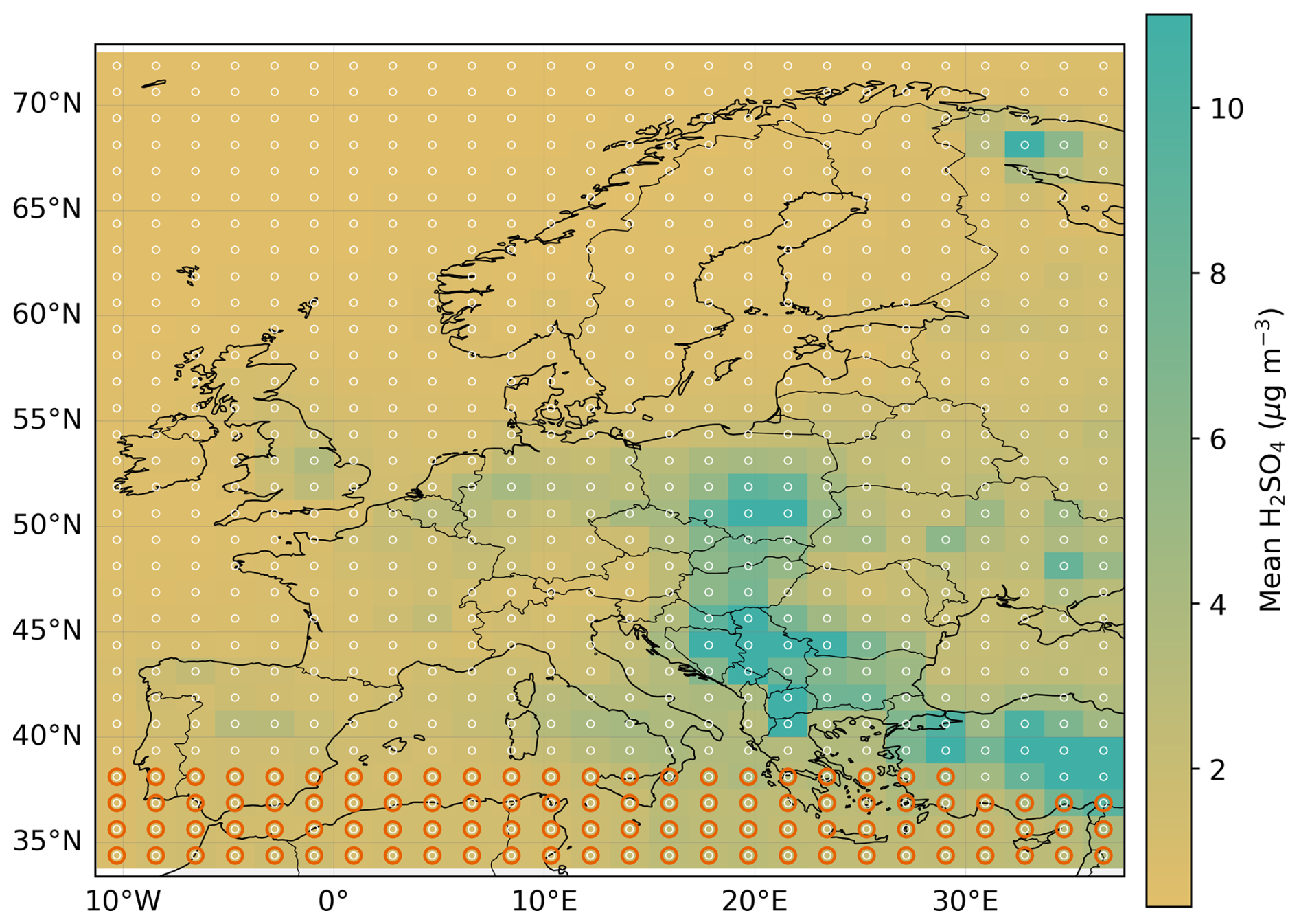
Figure 1 UKESM1 PPE domain using one example target variable: mean H₂SO₄ concentration (µg m⁻³) for January 2017. The map shows the European domain with grid points centers marked by white circles. Orange circles highlight the first 100 grid points selected for in-depth analysis in this work.

Figure 1 shows the UKESM1 PPE domain using one example target variable, the monthly mean H₂SO₄ concentration for January 2017. This illustrates both the spatial coverage of the European domain and the distribution of grid points required for emulator training and variance analysis. A subset of 100 model grid boxes was used to validate workflow performance before scaling to the full set of 9996 grid points for the optimised workflow.

2.1 Benchmarking setup

All performance tests were carried out on the JASMIN “LOTUS” high-performance computing (HPC) cluster hosted at the UK Centre for Environmental Data Analysis (CEDA) (Lawrence et al., 2013). The LOTUS cluster is a heterogeneous system with several thousand CPU cores available across multiple partitions. For this study, we used standard CPU nodes, each equipped with dual Intel Xeon processors (2.1–2.6 GHz) and 192 GB RAM, interconnected by high-speed InfiniBand. Jobs were scheduled using Slurm (v22.05), and all experiments were submitted through Slurm job arrays with task-level resource allocation. Unless otherwise noted, each task was executed on a single CPU core, and task submission was controlled using the #SBATCH - -array directive with a Slurm-array throttle (e.g. - -array=0-N%200). The value of 200 used throughout our scaling benchmarks was a deliberate production configuration choice rather than a hard limit of Slurm, the hardware, or the workflow. This throttle permits a maximum of 200 array tasks to run concurrently. Approximately 200 tasks generally executed concurrently under the benchmark configuration, although the number could occasionally be lower depending on resource availability and system load. The 10–16 GB value denotes the maximum memory requested per task and provides headroom for variability among grid cells and cases; actual memory consumption was lower and varied between tasks.

Original dataset sizes mirrored those used in the scientific analysis such as those reported in Regayre et al. (2026, 2023), Lee et al. (2012, 2016), and Johnson et al. (2020), though analyses were restricted in those studies. For benchmarking purposes, we measured end-to-end walltime, peak memory usage, and accuracy equivalence across both the currently used (baseline) and newly developed (optimised) workflows. Accuracy was quantified using Pearson correlation and root mean squared error (RMSE) between baseline and optimised outputs, while scalability was assessed as a function of task count and concurrency level. Default walltime limits were set to 24 h for all experiments, with memory limits varied between 10 and 32 GB per task depending on workload.

All software were used in stable production releases available at the time of analysis. Python (v3.10) was used for pipeline orchestration, plotting, and baseline GAM fitting with pyGAM (v0.9.0) (Servén et al., 2018). R (v4.2.2) (R Core Team, 2022) was used for GP emulation with DiceKriging (v1.6.0) (Roustant et al., 2012) and for optimised GAM fitting via mgcv (v1.8-41) (Wood et al., 2015). Additional R packages included readr (Wickham and Bryan, 2023), lhs (Carnell, 2022), sensitivity (Pujol et al., 2017), trapezoid (Sottile and Gohel, 2022), and truncnorm (Mersmann, 2022). Parallelisation was supported by Slurm job arrays on the cluster side, and OpenMP (v4.5) within mgcv::bam() for multithreaded GAM fitting.

2.2 Baseline workflow and bottlenecks

2.2.1 Baseline GP emulation

The baseline workflow combined GP emulation and GAM fitting using widely available Python libraries. GP emulators were trained with the scikit-learn GaussianProcessRegressor using a squared-exponential kernel with automatic relevance determination. Training was performed sequentially, with one emulator fitted per parameter setting, and relied on dense kernel inversions that scale cubically with the number of training points. Although individual emulators were modest in size, the aggregate cost of fitting tens to hundreds of thousands of models became prohibitive. Intermediate emulator outputs were written to disk for subsequent analysis, introducing additional input/output (I/O) overhead.

2.2.2 Baseline GAM fitting

GAM fitting was carried out entirely in Python using the pyGAM library with cubic regression splines. Fits were implemented serially at the grid box level, with each requiring repeated construction of large design matrices and independent smoothing‐parameter optimisation. This approach was straightforward to implement and completely reproducible, but computationally inefficient as no batching or parallelism was possible, and memory was not shared across tasks.

Figure 2 Measured runtime distribution of the baseline workflow over 100 operations.

To clarify the distinct role of the GAM within the overall workflow, we briefly describe its relationship to the GP emulator. The GP emulator is first used to approximate the model response and generate a dense sampling of the 37-parameter space based on output from the original 221-member PPE. This dense sampling provides a smoother and more complete representation of the response surface. At the grid-box scale considered here, model responses are often highly non-linear and spatially heterogeneous, so fitting a GAM directly to the sparse PPE would provide only a coarse and potentially noisy estimate of parameter effects. The emulator-expanded sample therefore provides a more robust basis for variance decomposition and sensitivity analysis.

While a GAM fitted directly to the original PPE is computationally inexpensive and can be performed without HPC resources, it remains constrained by the limited sampling density of the parameter space. In contrast, the GP emulator enables efficient generation of a much larger ensemble (order 10⁶), providing a more complete representation of the response surface. Fitting a GAM to this extended dataset becomes both memory-intensive and computationally demanding, motivating the need for the parallel HPC-based workflow developed in this study.

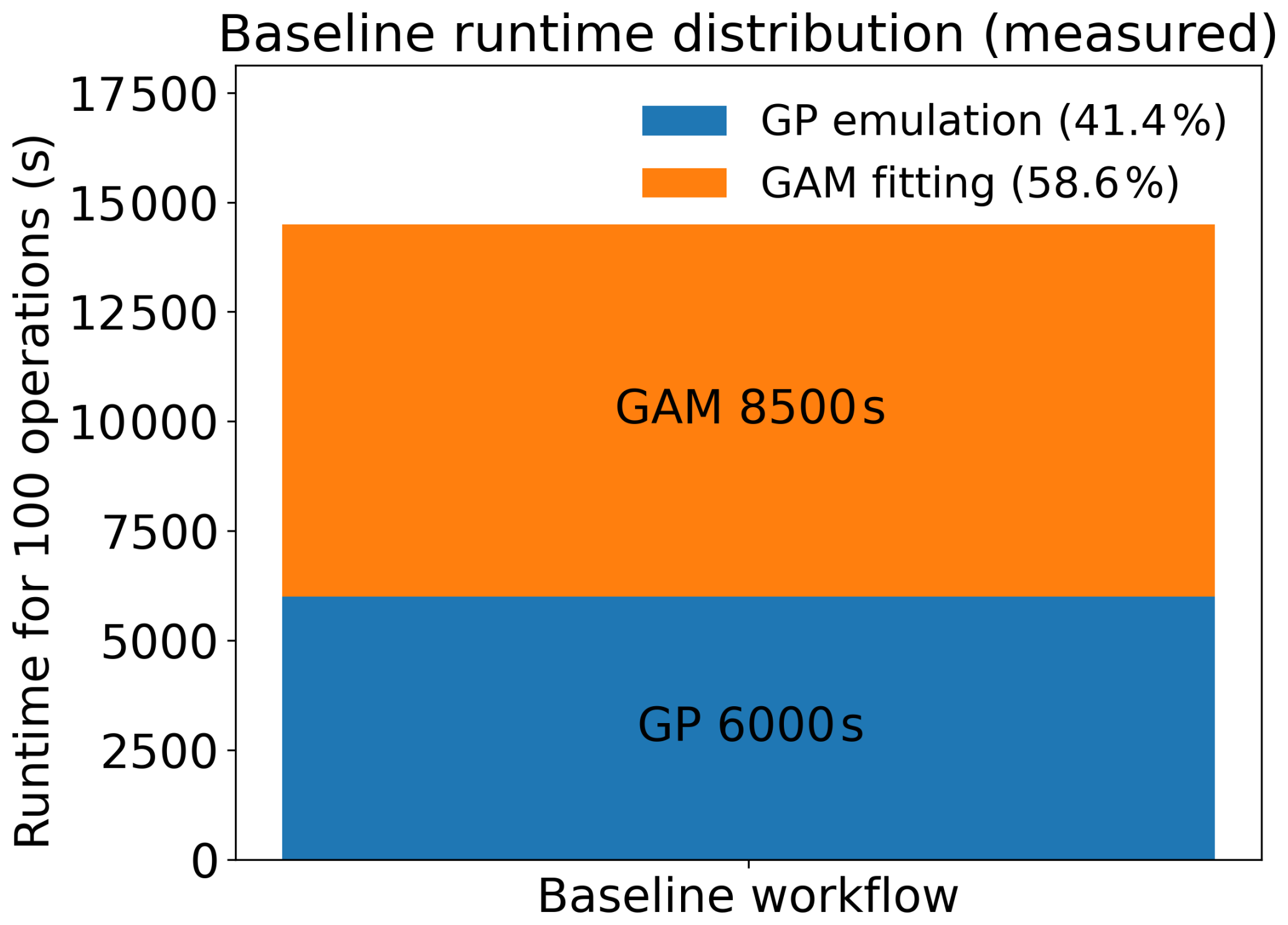
Figure 2 summarises the runtime profile of the baseline workflow and shows that GAM fitting for one million combinations across 37 parameter dimensions dominated total runtime. GAM fitting was also the main contributor to peak memory use. In the baseline implementation, which uses pyGAM, memory usage within a single process regularly exceeded 80 GB during spline matrix assembly, reflecting the cost of constructing large design matrices in memory. In contrast, the optimised workflow employs rBAM, which is substantially more memory-efficient and enables block-wise computation and distributed execution across independent tasks. This allows each task to operate within the typical 10–16 GB memory allocation, making the approach well suited for large-scale parallelisation.

Across 100 operations, GAM fitting required ∼ 8500 s (58.6 % of total wall time) and GP emulation ∼ 6000 s (41.4 %), giving a total of ∼ 14 500 s. Disk I/O overhead was negligible at this scale but becomes significant at larger ensemble sizes due to the churn of intermediate files.

2.2.3 Baseline (median-hold) variance computation

In the baseline implementation, the marginal importance of each parameter was obtained by a “median-hold” procedure. For each parameter x_i, the multi-dimensional GAM model predictions were recomputed while varying x_i across the extended ensemble and holding all other parameters fixed at the median values used to train the GAM.

The variance of the resulting one-dimensional prediction series quantifies the sensitivity of the model response to changes in x_i. This quantity provides a measure of first-order marginal importance for each parameter. It is analogous in interpretation to an unnormalised first-order Sobol-type sensitivity measure under an additive (no-interaction) assumption, as each parameter is varied independently while all others are held fixed (Sobol', 2001; Saltelli et al., 2008). It is not a formal Sobol index, as it is not normalised by the total variance and does not include higher-order interaction effects.

Repeating this process for all 37 parameters yields a set of per-parameter variances Var(f_i) and gradient signs given by sign[Cov(x_i,f_i)], which can be compared to quantify the relative importance of model parameters in driving output variance.

Although this approach is conceptually straightforward, it requires rebuilding the prediction matrix P times (once per parameter) and is therefore computationally expensive. The baseline workflow had three bottlenecks. First, GP emulation ran as a loop-based wrapper with dense-kernel inversions executed sequentially, leaving the embarrassingly parallel PPE analysis structure under-utilised. Second, GAM fitting in pyGAM was serial, using cubic splines with cross-validation smoothing, which scaled poorly with the number of grid boxes and caused repeated disk access. Third, the stages communicated via per-grid text .dat files, creating tens of thousands of small files and heavy metadata traffic on the shared file system. On the JASMIN super-data-cluster, where jobs are limited to 36 h and 64–128 GB per node, these bottlenecks led to 20–30 h runtimes for a single large-scale experiment and frequent out-of-memory failures.

3 Optimised workflow

The optimised pipeline targets the dominant computational costs identified in the baseline workflow: GP emulation and GAM fitting. The key design principle is to preserve the statistical formulation while restructuring execution and data handling to enable high concurrency, bounded memory usage, and minimal I/O.

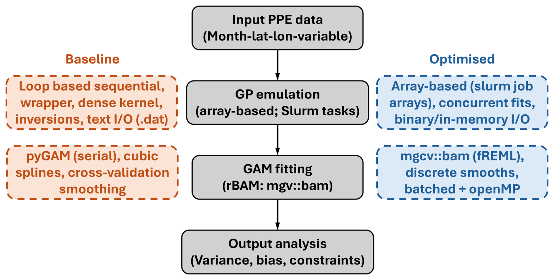
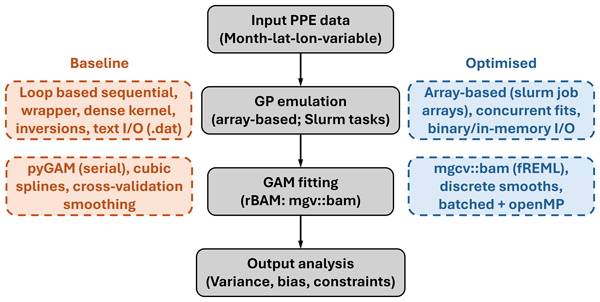
Figure 3 Schematic comparison of the baseline and optimised workflows. Grey boxes show the main workflow stages; orange boxes indicate baseline implementations; blue boxes indicate optimised implementations. The optimised workflow differs from the baseline in task execution, data handling, and prediction matrix construction. The GP emulation stage trains a Gaussian Process emulator for each grid box and generates one million parameter samples per emulator. The GAM fitting stage applies generalised additive models to the emulated outputs to decompose variance and identify parameter sensitivities.

The optimisation is not limited to replacing a sequential loop with Slurm job arrays. Rather, it involves a restructuring of the workflow, including changes to task execution, data flow, and prediction matrix construction. Job arrays serve as an enabling mechanism for parallel execution, but the primary gains arise from eliminating competing processes, reducing I/O overhead, and avoiding repeated recomputation of large intermediate data structures.

Across the full workflow, these changes yield an overall speed-up of ∼ 25 × (96 % total runtime reduction) and reduce peak memory by a factor of 12, with outputs matching the baseline to numerical tolerance. Figure 3 summarises the end-to-end process; implementation details are given below and a baseline–optimised comparison is provided in Table 1.

3.1 Optimised Gaussian process emulation stage

In the baseline workflow, GP surrogates were trained and evaluated using serial loops that spawned multiple competing Rscript processes on a single node. This resulted in inefficient CPU utilisation, repeated construction of prediction matrices, heavy disk-based I/O through large text intermediates, and straggler tasks that delayed completion.

The optimised implementation retains the same emulator formulation (DiceKriging::km) and large-sample prediction approach. However, it restructures execution and data handling. A task table is constructed such that each (month, latitude, longitude) combination maps to a single independent task executed via a Slurm job array. This ensures deterministic task assignment, isolates failures for straightforward re-submission, and enables cluster-wide concurrency.

This optimisation is not limited to replacing a loop with Slurm job arrays; rather, it involves a restructuring of execution, data flow, and prediction matrix construction. In addition to task-level parallelisation, several key changes are introduced. First, competing Rscript processes are eliminated by assigning one emulator per task, avoiding contention within a node. Second, large intermediate files are avoided by replacing text-based I/O with in-memory data transfer or compact binary output, substantially reducing filesystem overhead. Third, prediction matrix construction is reorganised to minimise repeated recomputation, reducing both runtime and memory pressure. Together, these changes convert the GP emulation stage from a sequential, I/O-bound workflow into a scalable, task-parallel process with bounded per-task memory usage.

Validation tests at representative grid points confirmed that the baseline and optimised workflows produced effectively identical emulator outputs (Appendix B, Fig. B1), demonstrating that the optimisation preserves statistical fidelity while substantially improving computational performance.

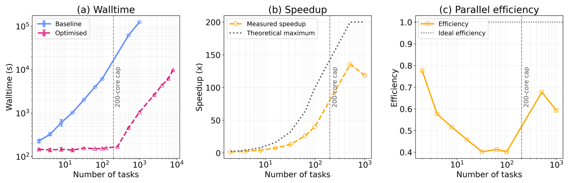
Figure 4 Scaling of the GP emulation stage. (a) Walltime as a function of the number of tasks (log–log scale) for the baseline (serial) and optimised (parallel) workflows. (b) Measured speedup relative to the baseline, compared with the theoretical maximum defined as $min(N,\mathrm{200})$, where N is the number of tasks and 200 is the array-task throttle. (c) Parallel efficiency, defined as the ratio of measured speedup to the theoretical maximum. The vertical dashed line indicates the 200-task throttle, beyond which tasks are processed in successive groups.

Performance scaling of the GP emulation stage is shown in Fig. 4. In the baseline workflow, runtime increases approximately linearly with the number of tasks, exceeding 6000 s for GP emulation in 100 grid boxes, consistent with a serial implementation based on a looped batch wrapper.

In the optimised workflow, one emulator is launched per Slurm array task, with up to 200 array tasks permitted to run concurrently. Task counts above 200 were executed in successive groups under this production configuration. The 200-task concurrency throttle was selected following preliminary testing as a stable and reproducible operating point on the shared LOTUS system. Approximately 200 tasks generally ran concurrently, whereas higher settings occasionally increased resource and filesystem contention and caused individual tasks to fail during periods of high system load. For task counts below this throttle, walltime remains approximately constant, indicating near-ideal parallel scaling; for larger task counts, walltime increases as tasks are processed in successive groups. To quantify the scaling behaviour, we define the theoretical maximum speedup as the minimum of the number of tasks and the 200-task throttle. Measured speedup is calculated as the ratio of baseline to optimised walltime, and parallel efficiency is defined as measured speedup divided by the theoretical maximum. At higher task counts, we performed additional baseline experiments at 512 and 1000 tasks to extend the comparison beyond the throttle. These results confirm the expected deviation from ideal scaling due to batching and scheduling overheads. At low task counts, the measured speedup approaches the theoretical maximum, reaching approximately 130 times faster than the baseline. Parallel efficiency decreases beyond the throttle and exhibits non-monotonic behaviour at large task counts, reflecting variability in walltime associated with HPC scheduling and I/O effects. Overall, the optimised workflow removes the sequential bottleneck in the GP stage, transforming the emulator workflow into a scalable, cluster-parallel process and enabling efficient utilisation of available HPC resources.

3.2 Optimised GAM fitting stage

In the baseline workflow, independent GAMs were fitted using pyGAM with cubic regression splines at each grid box. This required repeated construction of large design matrices and re-optimisation of smoothing parameters for every fit, resulting in high computational cost and memory usage for large ensembles. The optimised approach replaces this with an R-based Big Additive Model (rBAM), which is designed for efficient estimation on large datasets. In simple terms, the key change is that all parameter effects are evaluated simultaneously in a single pass, rather than recomputing model predictions separately for each parameter as in the baseline approach. This is achieved through fast restricted maximum likelihood (fREML) estimation, discrete smoothing, and multithreaded execution. In addition, the workflow is restructured to avoid repeated prediction and design-matrix reconstruction, allowing parameter contributions to be computed in a single batched (vectorised) operation. Together, these changes substantially reduce both runtime and memory requirements while preserving the statistical formulation of the model.

3.2.1 Vectorised variance and sign computation

After fitting the additive model

$$\mathit{\eta }=\sum _{i=\mathrm{1}}^P{f}_i\left(x_i\right),$$

we evaluate all partial effects simultaneously across the full dataset. In practice, this means that for each parameter x_i, the corresponding smooth contribution f_i(x_i) is evaluated at all N samples.

This produces a matrix

$$\mathbf{T}=[{\mathit{t}}_{\mathrm{1}},\mathrm{\dots },t_P],$$

where each column t_i represents the contribution of parameter x_i across all samples.

The marginal contribution of each parameter is then quantified using simple column-wise statistics:

$$\mathrm{Var}\left(t_i\right),\mathrm{sign}\left(\mathrm{Cov}\right(x_i,t_i\left)\right).$$

Here, Var(t_i) measures the strength of the parameter's influence on the model response, while sign(Cov(x_i,t_i)) indicates the direction of that influence.

This vectorised formulation computes all parameter effects in a single pass, rather than recomputing predictions separately for each parameter as in the baseline “median-hold” method. It therefore avoids repeated construction of design matrices and reduces computational cost from P prediction passes to one.

These quantities are invariant to additive constants in the partial contributions, since

$$\mathrm{Var}(t_i+c)=\mathrm{Var}\left(t_i\right),\mathrm{Cov}(x_i,t_i+c)=\mathrm{Cov}(x_i,t_i).$$

3.2.2 Implementation details

In practice, the matrix T is obtained using the predict(..., type="terms") functionality in mgcv, which returns the contribution of each smooth term evaluated across all samples. Computation is performed in blocks (via block.size) to control memory usage and combined with bam(..., discrete=TRUE) to enable efficient large-scale fitting. Parallelism is achieved both within each fit (via OpenMP multithreading) and across grid boxes (via Slurm job arrays).

3.2.3 Interpretation of the variance term

The variance term Var(t_i) represents the marginal contribution of parameter x_i within the full additive model. Each smooth function f_i(x_i) is estimated jointly with all others, so Var(t_i) reflects variability after accounting for the influence of the remaining parameters.

These quantities correspond to first-order marginal sensitivities and are directly comparable to the baseline median-hold approach. They should not be interpreted as total variance contributions, as interactions are not explicitly represented in the additive model. In particular,

$$\mathrm{Var}\left(\sum _i{f}_i\left(x_i\right)\right)=\sum _i\mathrm{Var}\left(f_i\right)+\mathrm{2}\sum _{i<j}\mathrm{Cov}(f_i,f_j),$$

so the sum of individual variances does not equal the total output variance.

This vectorised formulation reproduces the baseline results exactly while substantially reducing computational cost.

To verify that the optimised formulation preserves the statistical fidelity of the baseline workflow, we evaluate variance contributions across a broad spatial sample.

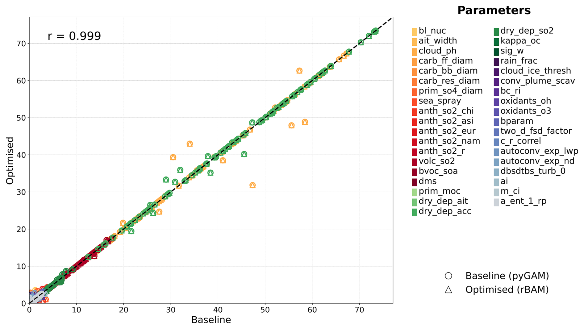
Figure 5 Comparison of fractional variance contributions from GAM fitting across 100 grid boxes (3700 points in total). Each point represents one parameter at one grid cell. The dashed line denotes the 1 : 1 relationship.

Figure 5 shows that variance contributions from the optimised rBAM workflow closely match those from the baseline pyGAM implementation across all grid boxes and parameters. The points lie tightly along the 1 : 1 line, with an overall Pearson correlation of r=0.999, demonstrating that the optimised approach reproduces the baseline variance decomposition with high fidelity across the domain.

Small deviations from the 1 : 1 relationship are visible for a limited number of parameters and grid boxes. These differences arise from numerical and algorithmic distinctions between the two implementations rather than any change in the underlying statistical formulation. In particular, pyGAM and mgcv::bam differ in spline basis construction, smoothing parameter estimation (cross-validation versus fREML), and numerical optimisation strategies. In addition, the optimised workflow employs discrete smoothing and block-wise evaluation of the prediction matrix, which can introduce minor numerical approximations at large sample sizes (∼10⁶). These effects lead to small local differences in estimated smooth functions, which propagate into slight variations in the derived variance contributions. However, these differences are small in magnitude and do not affect the overall ranking or interpretation of parameter importance. To provide additional context, the spatial distribution of correlation coefficients across all analysed grid boxes is included in the Appendix C (Fig. C1).

To quantify the computational benefits of this restructuring, we examine the scaling behaviour of the GAM fitting stage (Fig. 6). Panel (a) shows walltime, (b) the measured speed-up relative to the baseline, and (c) the corresponding parallel efficiency, together with the theoretical maximum scaling and the 200-task throttle.

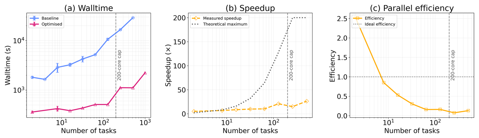
Figure 6 Scaling of the GAM fitting stage. (a) Walltime for baseline and optimised workflows, (b) measured speed-up compared to the baseline alongside the theoretical maximum (limited by the 200-task throttle), and (c) parallel efficiency defined relative to the effective concurrency. The vertical dashed line indicates the 200-task throttle. Deviations from ideal scaling at higher task counts arise from processing in successive groups beyond the throttle and from variability in resource availability on the shared system.

In the baseline workflow, runtimes increase superlinearly with the number of tasks, quickly exceeding practical limits beyond a few hundred grid boxes, while peak memory usage frequently approaches or exceeds node capacity.

In the optimised workflow, rBAM substantially reduces both runtime and memory requirements, achieving more than 20 times faster performance at approximately 10³ tasks. However, the scaling deviates from the theoretical maximum beyond moderate task counts. The 10–16 GB value represents the maximum memory requested per task and provides operational headroom for variation among grid cells and cases; it does not represent the memory continuously consumed by every task. Actual memory use was lower and varied between tasks, while approximately 200 tasks generally ran concurrently under the production configuration. Variability in resource availability and filesystem load on the shared LOTUS system nevertheless contributed to the observed flattening and fluctuations in speed-up and efficiency beyond ∼ 100 tasks.

Despite these practical constraints, the optimised workflow maintains substantially lower walltimes and improved efficiency compared to the baseline, enabling scalable application of GAM-based variance decomposition at resolutions and ensemble sizes that were previously infeasible.

3.3 Pipeline integration and reproducibility

The pipeline implements and automates the workflow for large-scale statistical emulation. In this context, the workflow refers to the ordered sequence of tasks required to generate, emulate, and analyse model output, specifically, GP emulation, GAM fitting, and downstream analysis. The pipeline, by contrast, is the software and organisational framework that executes this workflow reproducibly and efficiently on high-performance computing systems. It manages task scheduling, data handling, and parallel execution, ensuring that the workflow can be scaled and repeated without manual intervention.

The pipeline organises the optimised workflow around a task-centred folder layout with separate stages for GP emulation, GAM fitting, and downstream analysis. Configuration is provided via plain-text (.YAML/.JSON) files (month, grid, variable), enabling deterministic re-runs that reproduce identical results from the same inputs. A consistent file-naming scheme based on month, latitude and longitude indices supports automatic discovery of missing or failed tasks. In previous implementations, a single task failure, often caused by node timeouts or memory overuse, could halt or invalidate large batch jobs, requiring manual log inspection and reruns of the entire workflow. In the optimised pipeline, each task writes an individual log and output file identified by its coordinates, allowing a lightweight post-check script to detect missing or incomplete outputs and automatically resubmit only the affected tasks. This design prevents error propagation, eliminates manual recovery steps, and greatly improves overall robustness and throughput on HPC systems. Slurm job arrays orchestrate parallel execution for a given output variable, with each array index corresponding to a single model grid box for one month (one task). The array structure can span any number of grid boxes, regional or global, depending on available HPC resources. Inputs are read once per task; outputs are kept in memory or written in binary to limit I/O overhead. Per-task logs (slurm_output_%A_%a.out) record program outputs and error messages, and a lightweight post-check script scans for failures and automatically resubmits only the affected tasks.

Software environments are fully version-controlled to ensure reproducibility. All Python dependencies are specified in the Conda environment file envs/environment.yml, while all R packages (including mgcv and DiceKriging) are declared in the manifest script envs/install_R_deps.R. This script automatically installs the required packages from CRAN and records the complete R session information (sessionInfo()), providing an explicit record of the package versions used in the analysis. The workflow is designed to run efficiently on high-performance computing (HPC) systems (e.g., JASMIN, ARCHER) and can also be executed locally on Windows, Linux, or macOS. The repository includes a fully self-contained demonstration using four grid points (H₂SO₄, January 2017) that allows users to test the complete GP–GAM pipeline without requiring HPC access. Software environments are fully reproducible using the provided Conda specification (envs/environment.yml) for Python and the manifest script (envs/install_R_deps.R) for R.

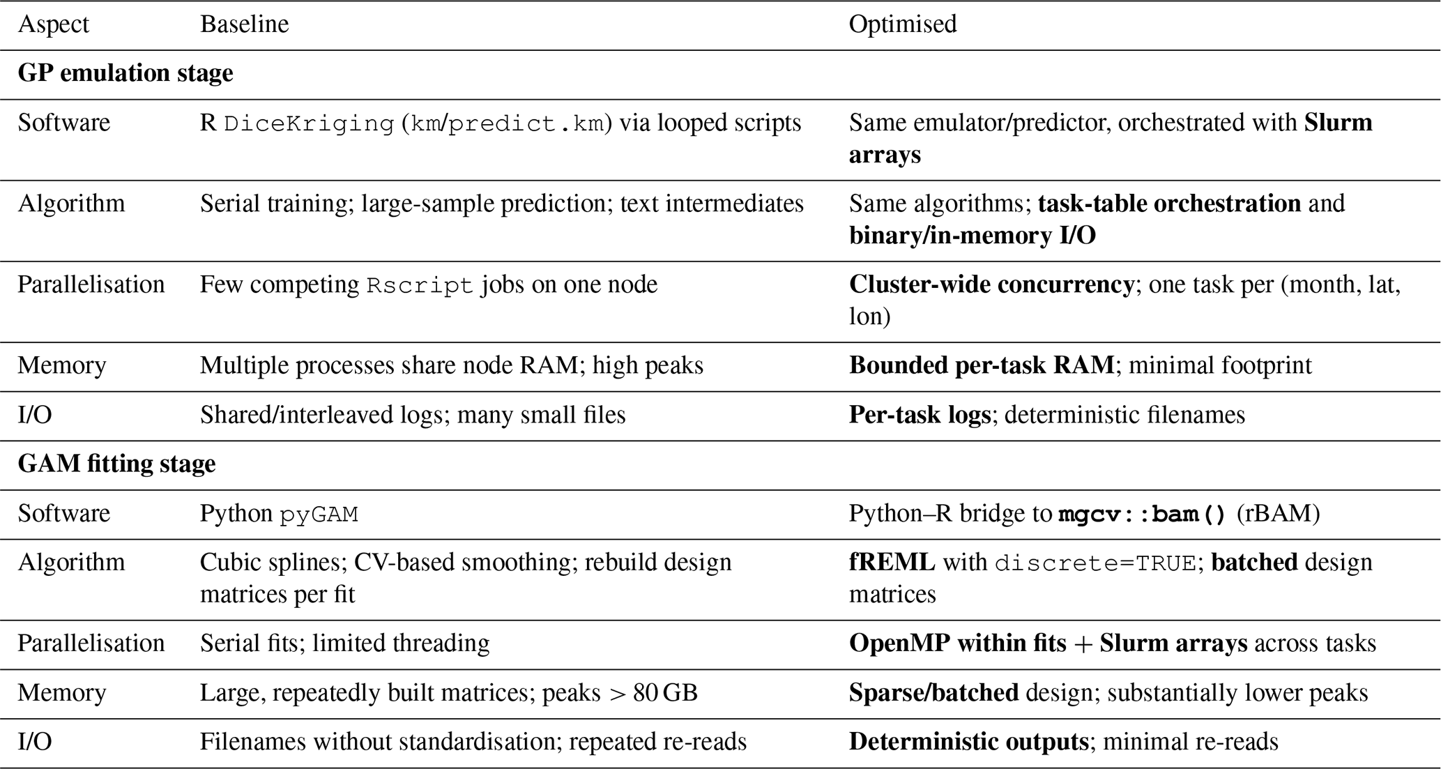
The individual improvements to GP emulation, GAM fitting, and workflow integration are brought together in Table 1, which contrasts key features of the baseline and optimised workflows.

Table 1 Baseline versus optimised workflows at the GP and GAM stages (key changes highlighted in bold).

4 End-to-end pipeline performance

The optimised workflow delivers large and systematic improvements in both runtime and memory at every stage of the pipeline (Fig. 7 and Table D1 in Appendix D). Median per-task walltime for the GP emulation falls from 6177 to 154 s (a 40.1× speed-up), while GAM fitting drops from 10 623 to 511 s (20.8×). Taken together, the end-to-end time reduces from 16 800 to 665 s – about 25.3× faster overall (from ∼ 4 h 40 min to ∼ 11 min per model grid box), for the 100-task benchmark case considered here.

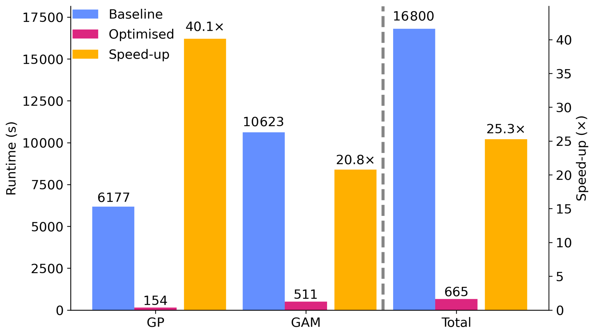
Figure 7 Bar chart of speed-up factors showing GAM fitting, GP emulation, and total pipeline side-by-side for quick comparison. Baseline and optimised runtimes (left axis) are shown alongside the speed-up (right axis). GP achieves the largest gain (40.1×; 6177 s → 154 s), GAM is 20.8× faster (10 623 s → 511 s), and the full pipeline is reduced by 25.3× overall (16 800 s → 665 s).

Peak memory usage shows comparable gains. GAM fitting, which dominated the baseline memory footprint, decreases from ∼ 100 to ∼ 10 GB (10.0× reduction), and the GP emulation stage falls from ∼ 50 to ∼ 6.5 GB (7.7×). As a result, the end-to-end peak memory requirement contracts by around 10.0×, enabling much denser job arrays on the same hardware and reducing the frequency of errors caused by memory limitations.

Practically, these improvements come from replacing slow, memory-intensive methods and I/O patterns with batched and streaming operations, using more efficient GAM fitting (e.g. discrete smoothing fits with bam) and lean GP emulation evaluation paths, while preserving the statistical specification of the original techniques. Figure 7 provides a side-by-side comparison of the GAM fitting, GP emulation, and total pipeline speed-ups to highlight where the largest gains are realised.

5 Application potential

The optimised pipeline substantially expands what is feasible in PPE-based climate model analysis. By reducing end-to-end runtime by more than an order of magnitude and lowering memory demand twelve-fold, our new workflow opens the door to in-depth analyses that were previously unachievable due to computational bottlenecks. In particular, four scientific areas of exploration are now enabled: (i) simultaneous treatment of multiple target variables, such as aerosol optical depth, cloud droplet number, and liquid water path, rather than single-variable case studies; (ii) finer temporal resolution, moving from annual mean to monthly, daily or even sub-daily outputs; (iii) extension to larger spatial domains, including global analyses without the need for coarse aggregation of model data; and (iv) cross-model comparisons in which multiple PPEs can be emulated and analysed under a unified statistical framework.

Example application scenarios include quantifying shared causes of aerosol radiative forcing uncertainty across multiple climate models, constraining interacting sources of uncertainty across model components and evaluating constraints across models to identify key structural model deficiencies in the current generation of climate models. The workflow is also readily applicable to non-climate large-ensemble settings where emulation and variance decomposition are required, such as hydrological forecasting, air-quality assessments or Earth system model evaluations.

Some opportunities for further refinement remain. We implemented discrete smoothing using rBAM, which significantly accelerates GAM fitting but may require parameter tuning when applied to extremely noisy or non-stationary predictors (not yet experienced in our chosen climate model outputs). Choice of kernel in GP emulator creation affects emulator fidelity – automated selection procedures could be implemented to trade some of the computation gains with improved emulator skill, which will be important as analyses scale. Finally, although per-task memory ceilings have been reduced substantially, very large multi-variable or multi-model applications, where distinct parameters are perturbed over model-specific ranges, will need more complex job-array design and, in some cases, access to distributed or GPU-enabled resources.

6 Conclusions

We have introduced and benchmarked a high-performance, open-source pipeline for large-scale statistical emulation in Earth system science. By restructuring workflow execution around task-level parallelism, streamlined I/O, and memory-efficient smoothing, we reduced GP training time by 97.5 % and GAM fitting time by 95.2 %, yielding a ∼ 25-fold end-to-end speed-up and a 12-fold reduction in peak memory demand. Crucially, these efficiency gains were achieved without loss of statistical fidelity, where emulator predictions and variance decompositions are numerically identical to the baseline implementation. The reduction in per-task memory is critical for enabling large-scale parallel execution across HPC systems, transforming PPE analysis from a memory-limited to a throughput-limited problem.

The workflow is designed for reproducibility and ease of adoption. All components are open-source, orchestrated via job arrays or containerised environments, and follow a deterministic file structure that simplifies reruns and failure recovery. This makes the pipeline directly reusable in other modelling contexts where emulators and smoothers are applied to high-dimensional outputs.

Future work will extend the framework in three directions: automatic kernel and smoothing-parameter selection to reduce the need for manual tuning, and distributed inference across heterogeneous HPC and cloud platforms. By combining statistical fidelity with computational tractability, the pipeline provides a scalable foundation for next-generation PPE studies and for broader applications of GP emulation and fractional variance decomposition methods in environmental science.

Appendix A: Lexicon of computational and workflow terms

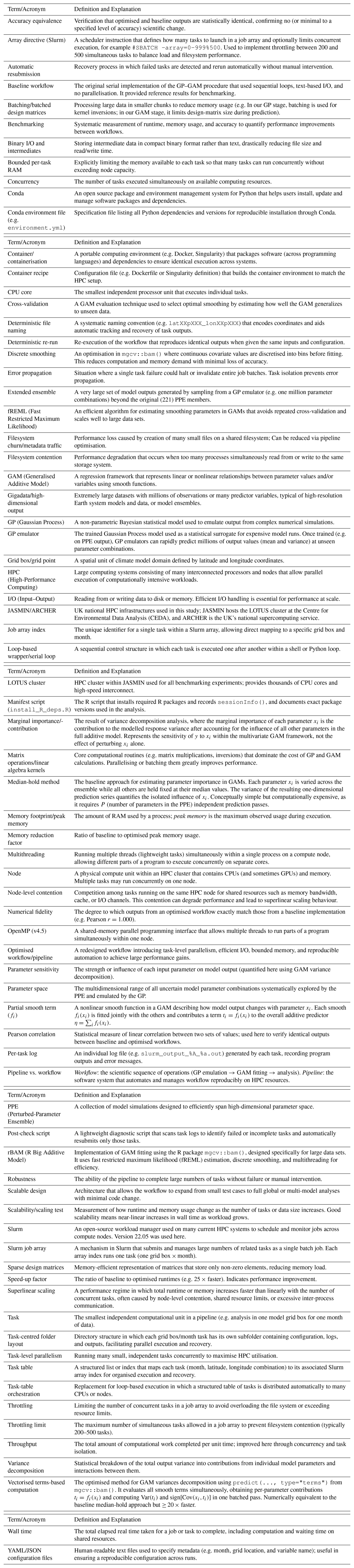
Table A1 This lexicon defines key computational and statistical terms used throughout the paper to aid readers who may be less familiar with high-performance computing and emulation workflow terminology.

Appendix B: Validation of GP emulator workflow optimisation

To confirm that the workflow optimisation did not alter emulator predictions, we compared probability density functions of mean H₂SO₄ at representative grid points for January 2017.

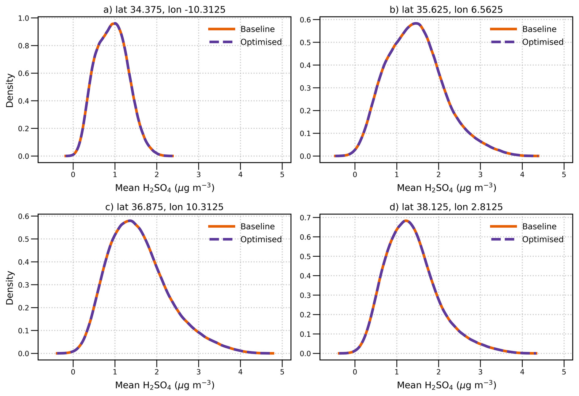
Figure B1 Probability density functions of mean H₂SO₄ for January 2017, obtained from one million parameter combinations using GP emulators. Panels (a)–(d) show results for four randomly selected grid points.

Appendix C: Spatial consistency of GAM variance decomposition

Figure C1 shows the spatial distribution of agreement between the baseline and optimised GAM variance decompositions across the analysed domain. For each grid box, the Pearson correlation coefficient is computed between the full set of parameter variance contributions derived from the two implementations. The results indicate consistently high agreement across the domain, with the majority of grid boxes exhibiting correlation coefficients close to unity. Out of the 100 grid boxes analysed, only four show a reduced correlation (r<0.99), highlighted in Fig. C1.

These localised deviations are consistent with the small differences observed in Fig. 5 and are attributable to numerical and algorithmic differences between the implementations, including spline representation, smoothing parameter estimation, and discretisation in the optimised workflow. The magnitude and spatial extent of these differences are limited, and they do not affect the overall interpretation of parameter importance. This spatial analysis supports the conclusion that the optimised workflow preserves the statistical behaviour of the baseline method across the domain.

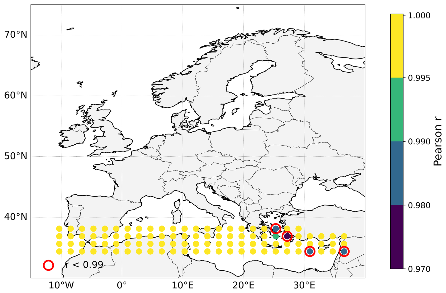
Figure C1 Spatial distribution of Pearson correlation coefficients (r) between baseline (pyGAM) and optimised (rBAM) variance contributions across 100 grid boxes for January. Each point represents one grid cell. Grid boxes with r<0.99 are highlighted with red circles.

Appendix D: Runtime and peak memory usage

Table D1 Runtime and peak memory usage for baseline and optimised pipeline, by stage and end-to-end. Speed-up and memory-reduction factors are calculated as baseline/optimised.

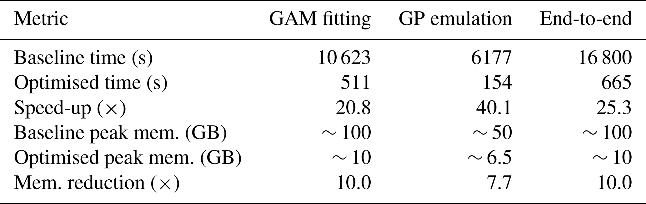
Notes: Times are median walltime across tasks; memory values are approximate peaks per task.