GPU-accelerated finite-element method for the three-dimensional unstructured mesh atmospheric dynamic framework

The three-dimensional unstructured-mesh finite-element atmospheric dynamical framework is gaining significance owing to its flexibility in representing complex topography and capability for multi-scale simulations in high resolutions. However, this framework has substantial bottlenecks. Unlike structured-grid models, the unstructured finite element method (FEM) must frequently access irregular mesh connectivity among nodes, edges, and elements, causing indirect memory addressing, inadequate data locality, and substantial memory bandwidth bottlenecks on conventional CPU architectures. Consequently, element-wise computations and global assembly are among the primary contributors alongside the sparse linear solver to the runtime in high-resolution simulations.

This study develops a GPU-parallel implementation of the Fluidity-Atmosphere dynamical core to address these challenges. The GPU-oriented data structures and optimized kernels are designed to efficiently leverage the computing power of GPUs. These kernels enable parallelized element integration and are efficient solvers for specific size matrices; a parallel assembly strategy enhances memory throughput during global sparse matrix construction. On the NVIDIA A100 GPU, the optimized kernels achieve speeds over 100× compared to the single CPU core baseline for element-wise computations and up to 389.02 times for global matrix assembly, resulting in an overall acceleration of 8.57 times with four messages passing interface (MPI) processes. The proposed framework demonstrates that tailored GPU parallelization is effective in overcoming the computational bottleneck of unstructured FEM-based atmospheric models, facilitating high-resolution simulations on heterogeneous architectures.

1 Introduction

Atmospheric dynamic frameworks are the fundamental tools for weather forecasting and climate simulation. In recent years, growing demands for the accurate prediction and management of extreme pollution and weather events have driven atmospheric models toward higher spatial resolutions and more sophisticated physical parameterizations. These advances create formidable computational challenges: doubling the spatial resolution can lead to exponential growth in computational cost, substantially increasing the demand for computing power and storage resources (Michalakes, 2020). For the discretization methods, the choice of scheme is primarily dependent on the topological structure of the underlying mesh. For high-resolution simulations, models are now able to resolve increasingly complex underlying surface features, such as terrains and urban structures. Owing to their geometric constraints, traditional terrain-following coordinate grids typically produce significant mesh distortions near steep terrain, introducing significant computational errors. Therefore, conventional atmospheric models based on structured “horizontal + vertical” grid configurations encounter inherent limitations in representing steep terrains, offering inadequate flexibility for localized adaptation.

To address this challenge, fully three-dimensional (3D) unstructured grids have emerged as an effective solution. Replacing the conventional quasi-3D approach that separates horizontal and vertical discretization, unstructured grids provide superior geometric adaptability and more flexible mesh generation capabilities (Smolarkiewicz et al., 2013; Szmelter et al., 2015; Giraldo, 2020; Tang et al., 2023; Tissaoui et al., 2023). The finite element method (FEM) proves particularly well-suited to such grid architectures, offering inherent advantages in handling complex geometrical configurations. This synergistic combination has established FEM as an increasingly prominent methodology in atmospheric modeling (Farrell et al., 2009; Kopera and Giraldo, 2014; Marras et al., 2015; Savre et al., 2016). FEM not only can be formulated to satisfy discrete conservation properties and numerical stability on irregular geometries but also enables local mesh refinement in critical regions, thereby improving simulation accuracy (Takle and Russell, 1988; Piggott et al., 2008; Müller et al., 2013; Huang et al., 2022; Kam et al., 2025; Gan et al., 2026a). To leverage these advantages, the Institute of Atmospheric Physics, Chinese Academy of Sciences, and AMCG group at Imperial College London jointly developed Fluidity-Atmosphere, a 3D adaptive atmospheric model (Li et al., 2021; Gan et al., 2026b). Based on the unstructured FEM, Fluidity-Atmosphere tightly couples the Navier-Stokes equations, complete advection-diffusion dynamics, and anisotropic adaptive mesh algorithms, facilitating dynamic mesh optimization during simulations to capture multi-scale flow phenomena.

However, while the FEM on unstructured meshes provides superior geometric flexibility, it also introduces inherent computational challenges that are absent in structured-grid models. In unstructured FEM frameworks such as Fluidity-Atmosphere, each element must frequently access irregularly connected nodes, edges, and faces during numerical integration and global sparse matrix assembly. This results in non-contiguous memory access, indirect addressing, and load imbalance across elements. These challenges are typically absent in structured grids, where data are stored in regular arrays with predictable access patterns. Moreover, the adaptive mesh refinement (AMR) feature of Fluidity-Atmosphere dynamically modifies the mesh topology during simulations, further complicating the memory layout. Consequently, the two most time-consuming components, namely, element-wise computations and global sparse matrix assembly, become dominated by irregular data movement rather than floating-point arithmetic, causing substantial memory bandwidth bottlenecks on CPU architectures (Sulyok et al., 2019).

Meanwhile, the slowdown of Moore's law and energy-efficiency bottlenecks of CPUs render CPU-only optimization inadequate for high-resolution simulations. In this context, GPUs have emerged as the widely used heterogeneous accelerators in high-performance computing. With massive parallelism and high-bandwidth device memory, GPUs have delivered orders-of-magnitude speedups in many numerical applications (Czarnul et al., 2020). For atmospheric models, particularly those based on FEM, computational intensity primarily arises from solving large-scale linear systems, parameterizing physical processes, and performing massive element-level operations, each amenable to GPU acceleration. Reengineering these components to run efficiently on GPUs has therefore become a key research direction.

Recent studies have reported significant advances in GPU acceleration of atmospheric models, including Navier-Stokes solvers (Goddeke et al., 2009; Thibault and Senocak, 2012), advection-diffusion equations (Simek et al., 2009), and iterative solvers for implicit schemes (Müller et al., 2015), typically with speedups of several orders of magnitude. Some Earth system models such as ocean model (Petersen et al., 2026), tsunami model (Conde et al., 2025), cloud-resolving atmosphere model (Bogenschutz et al., 2025) and sea-ice model (Jendersie et al., 2025) also were accelerated using GPUs. FEM modules such as numerical integration (Macioł et al., 2010; Sanfui and Sharma, 2020), matrix assembly (Kiran et al., 2020; Sanfui and Sharma, 2021), and linear solvers (Ratnakar et al., 2021; Kiran et al., 2020) have been explored, achieving speedups from tens to hundreds of times. Typically, the solution of large sparse linear systems is regarded as the dominant cost in FEM-based simulations and has been extensively studied, with numerous GPU-parallel implementations already achieving mature performance. However, the computation of elements and subsequent matrix assembly may pose significant challenges, primarily due to indirect memory addressing and low arithmetic intensity, particularly in large-scale unstructured atmospheric models. During each iteration, local element-wise matrices and right-hand sides must be computed and assembled into global sparse matrices. As the simulation domain expands, the number of mesh elements grows exponentially, leading to a proportional increase in computational cost. Without targeted optimization, the efficiency of the entire model can be substantially reduced.

In practice, element-wise computations and global matrix assembly involve frequent access to unstructured mesh data, where the topological relationships among points, edges, faces, and cells are maintained through multiple interlinked index arrays. These indirect data access operations disrupt spatial locality and cause irregular memory traffic, resulting in low cache utilization and high latency. Therefore, despite substantial progress in GPU acceleration of structured or semi-structured atmospheric models, unstructured FEM-based frameworks–characterized by irregular data dependencies and adaptive mesh refinement–still lack systematic and efficient GPU solutions. To address this research gap, this study focuses on the GPU parallelization and optimization of the two most time-consuming components of Fluidity-Atmosphere: element-wise computations (e.g., evaluating local mass and stiffness matrices via numerical integration) and global matrix assembly. The primary contributions are as follows.

1. GPU-based element-wise computations: Multiple optimization techniques are applied to accelerate compute-intensive kernels via GPU offloading, achieving more than 100× speedups compared with CPU versions.

2. GPU-based global matrix assembly: Parallel strategies are designed and implemented for element-wise assembly.

3. Integrated GPU implementation: The GPU kernels are integrated into Fluidity-Atmosphere with pinned memory to optimize data transfer. The results show that GPU kernels facilitate speedups exceeding two orders of magnitude, with 4 MPI processes and one GPU, achieving an overall acceleration of 8.57 times compared to a single CPU process.

The remainder of this paper is organized as follows. Section 2 introduces the program structure of Fluidity-Atmosphere, with emphasis on element-wise computations and global matrix assembly. Section 3 presents the GPU implementation and optimization of element-wise computations. Section 4 describes GPU-based global matrix assembly strategies. Section 5 evaluates the integrated GPU implementation and its performance. Section 6 concludes the paper, highlighting the future scope.

2 Target scientific application definition: fluidity-atmosphere

Fluidity-Atmosphere employs a mixed finite element/finite volume framework that incorporates the Navier-Stokes momentum equations, advection-diffusion equations for potential temperature and water vapor, and the compressible continuity equation within an anisotropic adaptive mesh algorithm. This design facilitates dynamic co-optimization of the mesh and physical fields. Fluidity-Atmosphere solves a coupled system of nonlinear equations with (typically) time-varying solutions. The time-marching algorithm employed uses a nonlinear iteration scheme known as Picard iteration in which each equation is solved using the currently optimal solution for the other variables. The dynamical framework supports both the continuous Galerkin (CG) and discontinuous Galerkin (DG) finite element formulations. This study is focused exclusively on the CG scheme. Specifically, in the performance evaluations and benchmarks presented in this study, the dynamic framework predominantly utilizes linear Lagrange elements (P₁) for the continuous Galerkin (CG) discretization. This choice inherently yields 4 degrees of freedom per tetrahedral element, resulting in the 4 × 4 local element matrices evaluated during the simulation.

Figure 1 Time loop of Fluidity-Atmosphere.

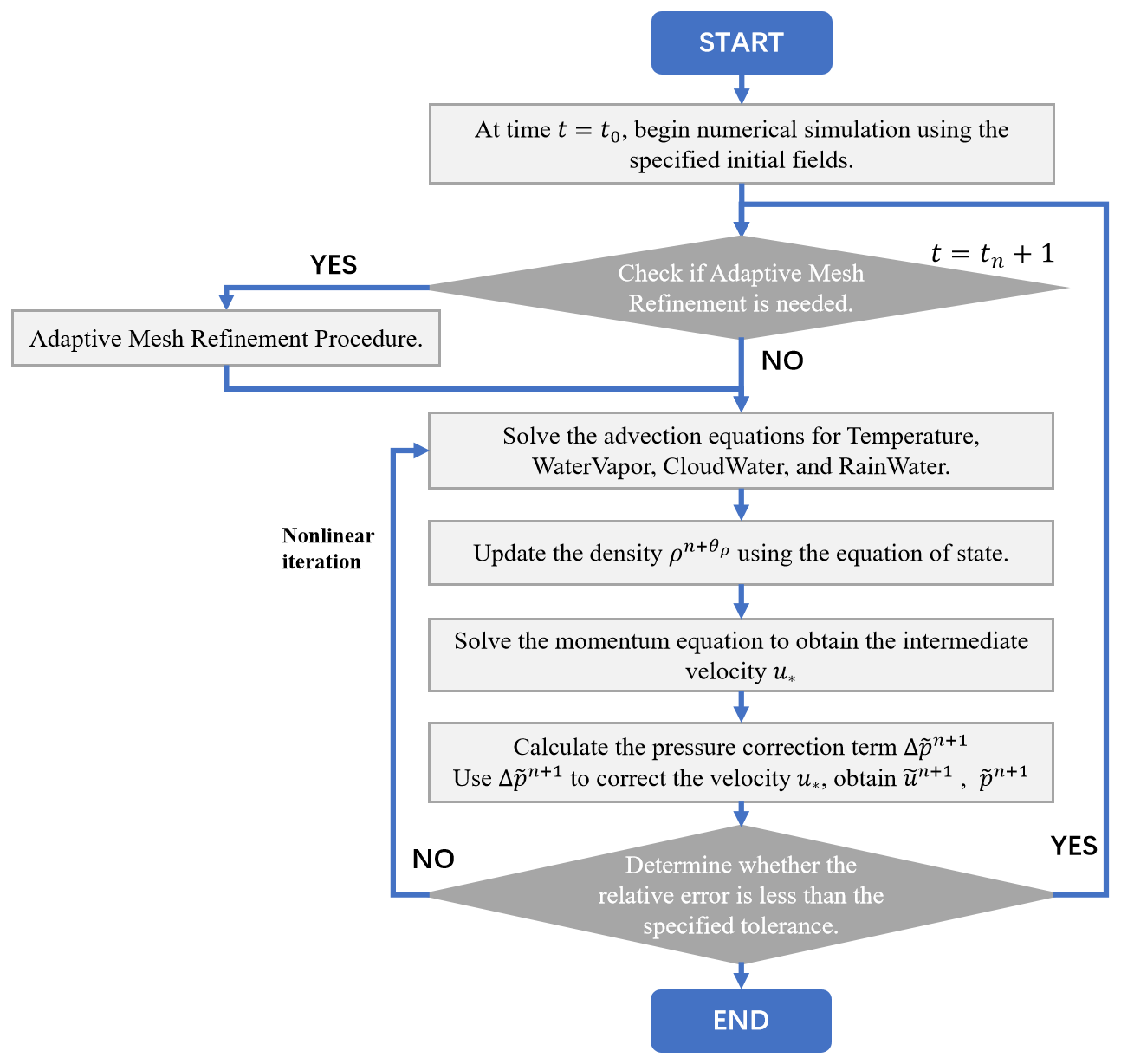
Figure 1 illustrates the general iteration loop of Fluidity-Atmosphere (Li et al., 2021). Fluidity-Atmosphere could invoke the adaptive algorithm at regular timesteps to ensure that the dynamics do not extend beyond the zone of adapted resolution. The adaptive algorithm has been parallelized using MPI processes, which run efficiently on CPUs. In our performance profiling, the nonlinear iterations were predominant. In each timestep iteration, the model solves governing equations such as the advection-diffusion and momentum equations. The processes of solving these equations in Fluidity-Atmosphere typically are divided into two major computational stages:

• 1.

  Construct matrices: For each element, numerical integration is performed using Gaussian quadrature to evaluate local stiffness, mass matrices, and right-hand side (RHS) vectors. These local contributions are subsequently inserted into the global sparse matrix system.

• 2.

  Solution of linear systems: The assembled sparse matrices are solved using parallel numerical libraries such as PETSc, employing iterative solvers and preconditioners well-suited for large-scale sparse problems. The PETSc library has good performance and scalability. In the simulated case studies, its contribution to the overall runtime was a significant portion (37 %) in the CPU-only baseline, and as detailed later, it becomes the dominant bottleneck once the matrix assembly is accelerated on the GPU. In addition, PETSc already supports GPUs (Mills et al., 2021). Hence, future studies will be focused on the integration of Fluidity-Atmosphere and PETSc GPU computing.

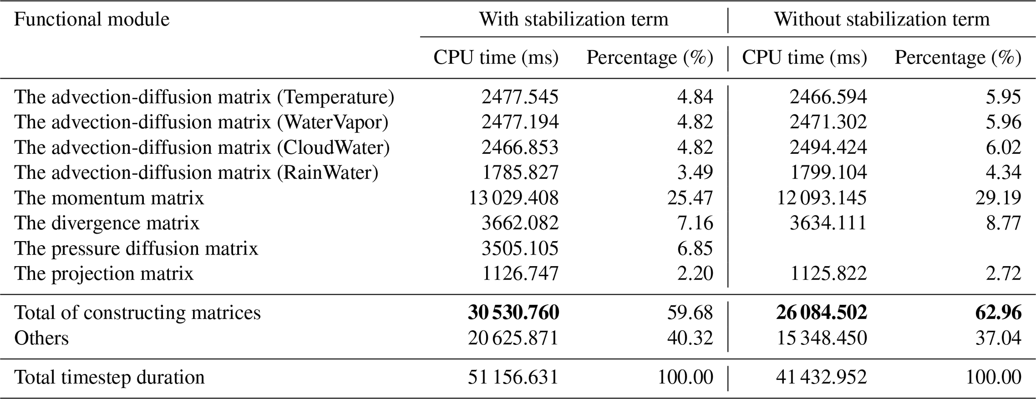
The computation times of constructing matrices contributes significantly to the overall runtime. For instance, in the Mountainwave3D simulation, the number of mesh nodes and mesh elements are 103 635 and 554 394, respectively. Table 1 shows the computational times of constructing matrices in a timestep. In particular, the pressure diffusion matrix is used to calculate the stabilization term, which is only calculated at the first timestep or when the grid changes because of the adaptive process. In the Mountainwave3D simulation, the pressure diffusion matrix is computed every ten time steps. Without calculating the stabilization term, the total time of the timestep will decrease, but the proportion of time required to construct the matrices will slightly increase. As quantified in Table 1, the processes of constructing matrices account for approximately 60 % of the total timestep duration in both scenarios (with and without the stabilization term). This high proportion confirms that accelerating element-wise computations and global assembly is the most effective strategy for improving the overall performance of the Fluidity-Atmosphere model.

The processes of constructing matrices share highly similar loop patterns. Hence, their general workflow can be summarized as follows:

• Step 1.

  Preparing Data: Initialize element mass matrices, right-hand sides, and local physical variables (such as velocity, density, and viscosity).

• Step 2.

  Coordinate transformation: The transform_to_physical function maps shape function gradients into physical space and computes Gaussian weights (detwei).

• Step 3.

  Setup test function.

• Step 4.

  Contribution evaluation: Call physics modules to accumulate contributions into element matrices and right-hand sides. Several functions, each corresponding to a distinct physical process, such as mass, advection, diffusion, source, and viscosity terms, are called. In addition to the calculation of physical variables, these functions extensively call the integration calculation function on the elements such as dshape_tensor_dshape, shape_dshape, and shape_shape. In the process of assembling the pressure diffusion matrix, a special function named get_edge_lengths (in which the small matrix solver is called) is used to calculate the element length scale in the physical space. All these functions are well-suited for GPU parallel computing.

• Step 5.

  Assembly: Local contributions are inserted into the global matrix and RHS. The subsequent irregular insertion operations into the global matrix makes it highly data-intensive and memory-bound. Owing to the massive throughput of GPU device memory, these functions can be accelerated on GPUs.

Therefore, the following sections describe the implementation and performance optimization methods of the element-wise computations and global matrix assembly on the GPU.

Although the current implementation is specifically optimized for the NVIDIA A100 GPU utilizing the CUDA programming model (NVIDIA, 2025a), the proposed optimization strategies are largely hardware-agnostic at the algorithmic level. Specifically, the element-wise parallelization strategy (one-thread-per-element), the data layout design, and the sparse matrix assembly workflow are general and can be applied to other GPU architectures.

Table 1 The computation times of constructing matrices. Bold values highlight the total computational time and percentage for the processes of constructing matrices.

However, certain implementation details rely strictly on CUDA-specific hardware features, such as double-precision atomic operations in the L2 cache, memory hierarchy optimization, and specific kernel launch configurations. Porting the implementation to other platforms, such as AMD GPUs, would primarily involve adapting CUDA-specific APIs to alternative frameworks like HIP (AMD, 2025). Since HIP provides similar abstractions for thread hierarchy, memory management, and atomic operations, the overall syntax porting effort is expected to be moderate.

Nevertheless, achieving true performance portability would require additional tuning to account for architectural differences in memory bandwidth, cache structure, and execution models. For instance, while NVIDIA V100 and A100 GPUs handle massive atomic updates highly efficiently, evaluating similar unstructured-grid applications on AMD CDNA architectures (e.g., MI100) has shown that standard atomic updates can incur higher penalties, sometimes necessitating alternative data restructuring or register-based aggregation to achieve optimal efficiency (Stone et al., 2021). Overall, the proposed algorithmic approach is expected to maintain its fundamental effectiveness across heterogeneous architectures, although achieving peak optimal performance on different platforms will inevitably require platform-specific tuning.

3 GPU parallelization of element-wise computations

In Fluidity-Atmosphere, element-level operations such as numerical integration and coordinate transformation constitute the core of unstructured finite element-wise computations. Profiling results indicate that these routines are invoked millions of times per timestep. Each nonlinear iteration involves re-evaluating element Jacobians, transforming basis functions, and accumulating physical contributions for all elements, which cumulatively dominate the computational workload. These observations identify numerical integration and coordinate transformation as the primary performance bottlenecks and thus the key focus of GPU parallelization in this study. The computation for each mesh element can be performed independently of others, making this step an ideal candidate for parallelization (Georgescu et al., 2013). GPUs feature a massively parallel processor architecture, which enables the simultaneous launch of a large number of parallel threads. These threads can be associated with different mesh elements to execute element-wise computations. These results are stored for subsequent assembly into the global matrix. Building on the workflow analysis in Section 2, this section presents the GPU implementation and optimization strategies for key subroutines, followed by a summary of general acceleration techniques.

Figure 2 Data layout of elements and variables.

3.1 Data structures and parallelization strategy

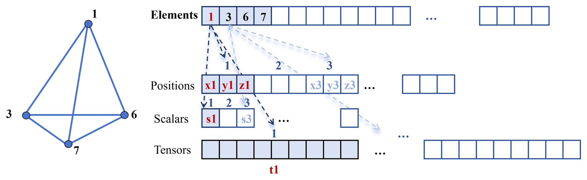
In unstructured meshes, element connectivity must be explicitly stored. Each tetrahedral element in Fluidity-Atmosphere records four vertex indices. Physical variables are stored in a unified Fields data structure organized as (number of vertices × dimension) arrays: scalars (1D), vectors (3D), and tensors (9D). The same layout is adopted in GPU memory to ensure contiguous access and consistent indexing (Fig. 2). Common fields such as density and temperature are stored as scalars, positions and velocities as vectors, and viscosity terms as tensors.

The element-wise computations in the FEM are intrinsically independent, making them particularly suitable for massively parallel execution on GPU architectures. Unlike spectral methods that involve global communication or high-order finite-difference schemes relying on extended stencils, finite-element computations are confined strictly within each element boundary. It is important to clarify that while Fluidity-Atmosphere utilizes a mixed CG/DG discretization, the GPU acceleration in this study focuses exclusively on the Continuous Galerkin (CG) operators (e.g., for the momentum and advection-diffusion equations). In the CG formulation, the numerical integration to evaluate local matrices remains mathematically entirely local. Unlike DG methods, which require calculating inter-element fluxes and jumps over facets, the CG element-wise computations do not introduce cross-element mathematical dependencies during the integration phase. The global coupling arising from shared mesh nodes is manifested exclusively during the global matrix assembly phase through indirect memory access.

This strong locality offers two principal advantages: (1) all element-wise computations can proceed independently, eliminating inter-thread communication during the compute phase; and (2) the workload is naturally balanced across elements, minimizing synchronization overhead. Consequently, a “one-thread-per-element” parallelization strategy is adopted. Each GPU thread handles one element. In our implementation, thread block sizes of 128 and 256 were both utilized, with the specific parameter for each kernel determined empirically via NVIDIA Nsight Compute. For the target mesh comprising 554 394 elements, a block size of 128 yields 4332 blocks, while 256 yields 2166 blocks. Given that the NVIDIA A100 GPU features 108 Streaming Multiprocessors (SMs), each with a theoretical maximum of 2048 resident threads, both configurations generate sufficient numbers of thread blocks to provide approximately 2.5 execution waves across the GPU, which helps maintain high occupancy and effectively hide memory latency.

3.2 GPU parallel coordinate transformation

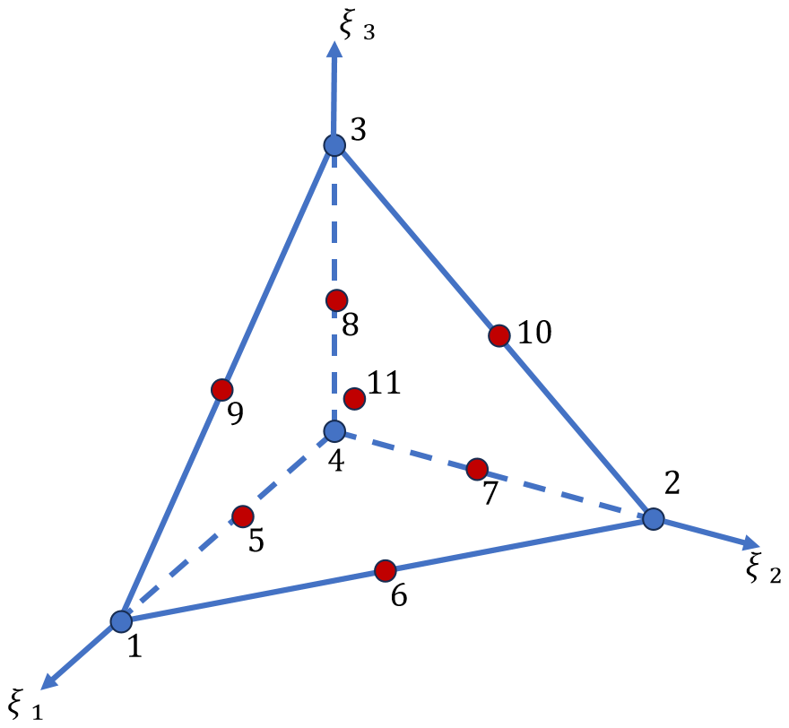
With the data layout on GPUs established, the next step is to implement the core finite element operation: coordinate transformation. Using a reference element (in this study, a tetrahedron), shape functions and Gauss points are consistently defined. In Fluidity-Atmosphere, each physical element employs 11 Gauss points: four vertices, six edge midpoints, and the centroid (Fig. 3). For each Gauss point, the transformation routine evaluates the integrand and multiplies it by the predefined weight.

Figure 3 The reference element and Gauss points.

Even though element-independent and theoretically parallelizable, this kernel is computationally intensive and one of the most frequently executed routines in the model. For every iteration and every element, it performs numerous small matrix operations: matrix multiplications, adjoint and determinant evaluations, and transformations of derivative matrices.

Algorithm 1 outlines the transform_to_physical procedure, where input and output arrays are stored contiguously to maximize memory efficiency. Crucially, the algorithm incorporates a conditional optimization for linear (P₁) elements: because standard affine mappings yield a constant Jacobian matrix, expensive operations (Jacobian construction, determinant, and inverse) are evaluated only at the first Gauss point (g_i=1) and cached.

Algorithm 1 Transform_to_physical.

Input: Element nodal coordinates X, shape functions N, reference derivatives ∇_ξN, Gauss points g_i

Output: Physical derivatives ∇_xN, weights detwei, J, J⁻¹, det J

for g_i=1 to n_gi  do

compute ∇_ξN(g_i)

if mapping is nonlinear or $g_i==\mathrm{1}$ then

construct Jacobian matrix $\mathbf{J}\leftarrow \mathbf{X}\cdot ({\mathbf{\nabla }}_{\mathit{\xi }}\mathit{N}{)}^T$

compute adj(J) and det J

normalize inverse matrix ${\mathbf{J}}^{-\mathrm{1}}\leftarrow \text{adj}\left(\mathbf{J}\right)/\det \mathbf{J}$

end if

transform to physical derivatives ${\mathbf{\nabla }}_x\mathit{N}\leftarrow {\mathbf{J}}^{-\mathrm{1}}\cdot {\mathbf{\nabla }}_{\mathit{\xi }}\mathit{N}$

compute quadrature weights $\text{detwei}\left(g_i\right)\leftarrow \left|\det \mathbf{J}\right|\cdot w_{gi}$

end for

The inner loop over Gauss points is deliberately retained to preserve framework generality for higher-order elements. Furthermore, rather than precomputing and storing these geometric quantities, which would exacerbate memory traffic in this heavily memory-bound framework, we employ a “compute-on-the-fly” strategy, trading abundant GPU arithmetic cycles to conserve precious memory bandwidth (Kronbichler and Kormann, 2012; Böhm et al., 2025).

3.3 GPU parallelization of element-wise integration

Element-wise integration routines constitute the computational core of unstructured finite-element models, as they are responsible for evaluating the contributions of each element to the global system. Profiling of Fluidity-Atmosphere indicates that these kernels are among the most frequently executed routines. During each nonlinear iteration, they are called once per element per physical equation, resulting in millions of invocations per timestep. As each call involves multi-dimensional tensor operations and numerical integration over multiple Gauss points, the accumulated cost dominates both the element-computation phase and the overall runtime of the model. Therefore, optimizing element integration is critical to achieving substantial end-to-end performance gains. The principal integration functions are as follows:

• dshape_tensor_dshape couples shape function gradients with tensor fields, supporting stabilization terms and physical field coupling.

• shape_shape integrates shape functions to construct the mass matrix, required in momentum and energy conservation equations.

• shape_dshape performs weighted integration of shape functions and their gradients at nodal points.

Among these functions, the dshape_tensor_dshape function is the most computationally intensive, as it involves both tensor-vector and vector-vector multiplications for every integration point. On the GPU, this procedure is parallelized at the thread level, with each thread processing one element. Beyond kernel-level parallelization, a series of GPU-specific performance tuning techniques are applied to completely exploit the hardware potential. These optimizations are guided by profiling by employing NVIDIA Nsight Compute, focusing on reducing memory latency, register pressure, and control overhead:

• Memory optimization: The __restrict__ qualifier is applied to pointer variables to eliminate aliasing and enable more aggressive memory-access optimizations. Small __device__ functions are annotated with __forceinline__ to reduce function-call overhead.

• Loop optimization: Loop-invariant expressions (particularly global memory accesses) are hoisted outside the loop body; manual loop unrolling or #pragma unroll directives are applied to innermost loops to reduce control overhead and increase instruction-level parallelism.

• Template metaprogramming: As the dimensions of the different matrices and vectors are already known at compile time, the __device__ functions such as matrix-matrix product and dot product are implemented as templates, facilitating the compiler to apply deeper optimizations for specific instantiations.

These measures are reflected in Nsight Compute reports as improved register utilization and reduced memory bottlenecks. Loop unrolling and templating yield substantial enhancements in small-scale computations. In combination with GPU-parallel element integration and small-matrix solvers, these optimizations form a cohesive strategy that maximizes performance while maintaining full consistency with the original CPU implementation.

It should be noted that the CPU baseline used for comparison represents the official, unmodified production code of Fluidity-Atmosphere, compiled with aggressive optimization flags -O3 -ffast-math. Under these flags, modern CPU compilers automatically apply substantial loop unrolling and vectorization. However, due to the warp-based execution model and strict register allocation of GPUs, the CUDA compiler frequently requires explicit manual directives (e.g., #pragma unroll) and compile-time size resolution (via templates) to achieve optimal instruction scheduling and register reuse. Thus, these GPU-specific manual optimizations are implemented to fully unlock the hardware's architectural potential rather than to introduce an algorithmic disparity. The optimized code is listed in Appendix A.

3.4 GPU parallelization of small-scale linear algebra solvers

In addition to numerical integration, the construction of stabilization terms involves numerous small-scale linear algebraic operations, such as solving 6 × 6 systems or computing eigen-decompositions of 3 × 3 matrices. Even though these operations are apparently lightweight, they are called repeatedly for every element and Gauss point, resulting in a substantial cumulative cost. On CPUs, relying on standard library routines such as LAPACK's DSPEV or Fortran's intrinsic solvers for these operations is highly inefficient. While a small 6 × 6 matrix easily fits into the L1 data cache, gathering these matrices from an unstructured mesh via indirect addressing disrupts spatial locality. Furthermore, these independent tiny matrices offer minimal opportunity for data reuse, limiting cache efficiency. From a software perspective, pre-compiled external library routines typically cannot be automatically inlined by the compiler within the tight element loop. Invoking them millions of times introduces profound function-call overhead, and their internal argument validation and branching dwarf the actual floating-point arithmetic.

To address this challenge, this study implements dedicated GPU-based small-matrix solvers and eigen-decomposition kernels as inline __device__ operators.

• Small linear systems (e.g., 6 × 6): These are solved on GPUs using Gaussian elimination. The input is an augmented matrix A (in column-major layout, including the right-hand side) with dimensions m×n. Pivoting and row exchanges are applied to control numerical errors, whereas column-major storage and in-place operations reduce register pressure and facilitate the alignment with GPU memory characteristics.

• Eigen-decomposition of 3 × 3 real symmetric matrices: Both iterative and direct GPU solvers are implemented, based on the methods employed in prior research. To improve efficiency, the implementation employs template-based array classes and includes sorting functions for eigenvalues and eigenvectors. By exploiting symmetry, only six entries (the diagonal and upper triangular part) are stored, minimizing register usage and avoiding spills to local memory.

These GPU-implemented solvers are lightweight and reusable across kernels. The modular __device__ design also promotes code reuse across physical modules and supports further fusion with integration kernels.

4 GPU parallelization of matrix assembly

In the FEM, matrix assembly serves as the critical bridge between local element-wise computations and the solution of global linear systems. As this stage involves extensive operations on sparse data structures and frequent memory access, it typically hinders the performance of the entire program. Therefore, migrating the matrix assembly procedure to GPUs and applying targeted optimizations is crucial for enhancing the computational efficiency of atmospheric models. This section introduces the global matrix storage formats, the element-wise parallel assembly strategy, and the GPU implementation of RHS vector assembly.

Before detailing our assembly strategy, it is worth noting that a prominent trend in high-performance finite-element simulations is to discard global matrix assembly in favor of matrix-free (or partially assembled) operator evaluations (Kronbichler and Kormann, 2012, 2019; Rudi et al., 2015). Matrix-free algorithms were fundamentally developed to address the performance bottlenecks inherent in high-order finite elements. In high-order discretizations, full matrix assembly leads to an exponential explosion in memory footprint and floating-point operations per degree of freedom (DoF). Matrix-free approaches, typically coupled with sum factorization, suppress this complexity, thereby drastically increasing computational intensity and parallel efficiency (Fischer et al., 2020).

However, the dynamic framework evaluated in this study predominantly employs low-order linear elements (P₁). For low-order FEM, the memory access per DoF is intrinsically small and remains comparable whether using fully assembled operators or on-the-fly matrix-free evaluations. Since low-order evaluations are heavily memory-bound, transitioning to matrix-free methods does not yield the profound bandwidth savings observed in high-order regimes. Furthermore, explicitly assembling the global sparse matrix provides a critical advantage: it enables the use of highly optimized, generic Sparse Matrix-Vector multiplication (SpMV) kernels and sophisticated algebraic preconditioners, such as Algebraic Multigrid (AMG) and Incomplete LU (ILU) provided by PETSc, which are indispensable for the stability and efficiency of the implicit time-stepping solvers in Fluidity-Atmosphere. Therefore, accelerating the global sparse matrix assembly remains the most rational and impactful optimization pathway for this class of low-order dynamical cores.

4.1 Global matrix assembly

Following local integration, the algorithm accumulates (A^e, F^e) into the global matrix A and vector F according to the connectivity information of the mesh. This procedure, widely recognized as the global assembly, transforms element-level contributions into a consistent global representation based on the mapping between local and global degrees of freedom, as shown in Algorithm 2. Here, ε is the set of elements and e is an element. The elem function performs element-wise computations to get element matrices. The L function retrieves the node numbering.

Algorithm 2 The Global Matrix Assembly.

Output: Global matrices A, F

Initialize A, F to zero

for all e∈ε do

Compute $({\mathbf{A}}_e,{\mathit{F}}_e)=\text{elem}\left(e\right)$

for all local degrees of freedom d₁ of e do

$\mathit{F}\left(L\right(e,d_{\mathrm{1}}\left)\right)+={\mathit{F}}_e\left(d_{\mathrm{1}}\right)$

for all local degrees of freedom d₂ of e do

$\mathbf{A}\left(L\right(e,d_{\mathrm{1}}),L(e,d_{\mathrm{2}}\left)\right)+={\mathbf{A}}_e(d_{\mathrm{1}},d_{\mathrm{2}})$

end for

end for

end for

In contrast to structured-grid models, where mesh nodes are arranged in a regular $(i,j,k)$ indexing order and memory access can be performed sequentially and predictably, unstructured meshes lack geometric regularity. The connectivity of each element varies depending on its neighbours, and the mapping between local and global indices must be retrieved indirectly through lookup tables. Consequently, the assembly phase in unstructured FEM involves frequent non-contiguous global memory reads and writes, with irregular strides between consecutive memory locations. This destroys spatial locality and drastically increases cache miss rates, thereby amplifying the ratio of memory access time to floating-point computation.

On GPU architectures, these irregular access patterns exacerbate performance degradation. Concurrent threads typically need to update overlapping entries of the global sparse matrix, requiring synchronization or the use of atomic operations to ensure correctness. The combined effects of irregular global memory traffic, low cache reuse, and write conflicts make matrix assembly a highly memory-bound process.

Consequently, global matrix assembly presents two major challenges: (1) the imbalance between memory traffic and arithmetic intensity, caused by the dominance of irregular global data movement over computation; (2) the difficulty of ensuring data consistency during concurrent updates. Cumulatively, these factors make matrix assembly another critical performance bottleneck, and thus a central focus of GPU parallel optimization in this work.

4.2 Sparse matrix storage formats

Fluidity-Atmosphere employs different sparse storage formats for different types of physical fields. For scalar field matrices, the compressed sparse row (CSR) format is used. For vector field matrices such as three-component velocity, the block-CSR (BCSR) format is adopted.

For a scalar field, the local stiffness matrix can be expressed as Eq. (1):

$$\begin{array}{}\text{(1)}& K_{ij}=\underset{{\mathrm{\Omega }}_e}{\int }\left(\mathbf{\nabla }{\mathit{N}}_i{)}^T\mathbf{C}\right(\mathbf{\nabla }{\mathit{N}}_j)\mathrm{d}\mathrm{\Omega }\end{array}$$

where N_i and N_j are basis functions, Ω_e is the integration domain of the element, and C is the associated tensor. For scalar fields, N_i is a scalar and K_ij is a scalar integral, resulting in a 4 × 4 local element matrix. By obtaining the global node indices n_i and n_j corresponding to the local nodes i and j, the result K_ij is updated in the global matrix entryy(n_i,n_j).

The global matrix is typically stored in the CSR format, which consists of three arrays: values (non-zero entries), col_index (column indices), and row_pointers (row offsets) (NVIDIA, 2025b). Within a row range, the target column can be located using binary search.

For vector fields, each node contains three degrees of freedom (DOFs). Thus, while assembling the local stiffness matrix, all interactions among the nodes and their DOFs must be considered. This results in a set of 4 × 4 blocks, each of size 3 × 3:

$$\begin{array}{}\text{(2)}& \mathbf{K}=\left[\begin{array}{cccc}{\mathbf{K}}_{\mathrm{11}}& {\mathbf{K}}_{\mathrm{12}}& {\mathbf{K}}_{\mathrm{13}}& {\mathbf{K}}_{\mathrm{14}}\\ {\mathbf{K}}_{\mathrm{21}}& {\mathbf{K}}_{\mathrm{22}}& {\mathbf{K}}_{\mathrm{23}}& {\mathbf{K}}_{\mathrm{24}}\\ {\mathbf{K}}_{\mathrm{31}}& {\mathbf{K}}_{\mathrm{32}}& {\mathbf{K}}_{\mathrm{33}}& {\mathbf{K}}_{\mathrm{34}}\\ {\mathbf{K}}_{\mathrm{41}}& {\mathbf{K}}_{\mathrm{42}}& {\mathbf{K}}_{\mathrm{43}}& {\mathbf{K}}_{\mathrm{44}}\end{array}\right].\end{array}$$

Each element of the element matrix K_ij is actually a 3 × 3 matrix.

$$\begin{array}{}\text{(3)}& {\mathbf{K}}_{ij}=\left[\begin{array}{ccc}a& b& c\\ d& e& f\\ g& h& i\end{array}\right].\end{array}$$

Here, Fluidity adopts the BCSR format, which is structurally similar to CSR, but stores continuous block data in the value array. This block-based representation better supports sparse operations for vector fields.

4.3 GPU parallel element-wise assembly

In our GPU parallelization, the contributions of each mesh element are computed and stored in parallel, with each GPU thread responsible for one element. A dedicated kernel is launched to assemble element matrices.

In the implementation, each thread iterates over the entries K_ij of the local element matrix and looks up the corresponding global non-zero indices. Given the global node indices n_i and n_j, the row_pointers array is first used to locate the row range [row_pointers(n_i), row_pointers(n_i+1)). Within this range, the column index n_j is searched using binary search. To enhance the efficiency, the implemented GPU assembly function consistently adopts binary search.

A significant challenge arises during parallel write-back, where race conditions may occur if multiple threads attempt to update the same non-zero entry simultaneously. An atomic operation is indivisible and guarantees consistency by preventing interference from other threads. Modern GPUs provide hardware-level support for atomic addition, enabling conflict-free concurrent updates without explicit locks. In this work, the atomic add approach is adopted for its efficiency and simplicity. The CUDA parallel assembly code is listed in Appendix B.

To summarize the complete execution pipeline, the global matrix assembly occurs entirely within the GPU device memory. Following the element-wise computations, the local element matrices are accumulated into the global sparse matrix arrays (i.e., the values array in CSR/BCSR format), which are pre-allocated on the GPU. This is achieved using the aforementioned parallel assembly kernel equipped with hardware-level atomicAdd operations. Upon the completion of the assembly kernel, the fully constructed global matrix arrays are transferred back to the CPU host memory via PCIe. The assembled matrix is then handed over to the CPU-bound PETSc library to perform the subsequent large-scale linear system solve.

4.4 GPU parallel assembly of Right-Hand-Side (RHS) vectors

Similar to the global matrix, the RHS vector is assembled using an element-wise parallel strategy. Each GPU thread computes the nodal contributions of one element and accumulates them into the corresponding global vector entries.

The implementation first determines the indices of the nodes belonging to each element, then loads the nodal values, and finally applies atomicAdd operations to ensure correctness during concurrent accumulation. For cases where multiple variables are associated with a node, appropriate offsets are added to the corresponding positions. The Appendix C illustrates the procedure of RHS assembly, which achieves efficient large-scale parallel accumulation while preserving correctness.

5 Results and evaluation

5.1 Experimental environment

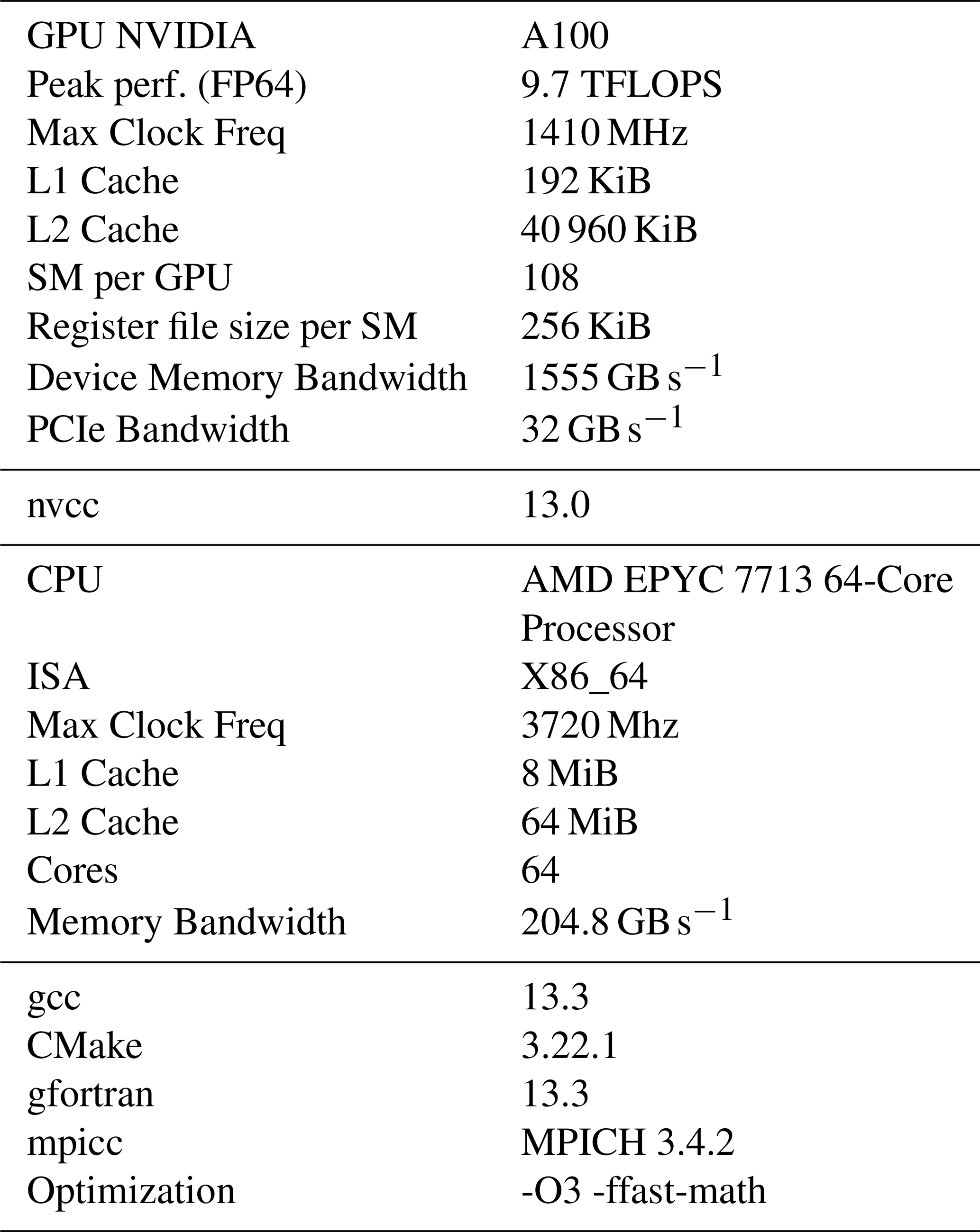
This section presents a systematic analysis of the performance of the proposed GPU parallelization strategies. Experiments were conducted to first validate correctness on both CPU and GPU platforms, and then to evaluate performance in four aspects: element-wise computation, global matrix assembly, data transfer with computation overlap, and overall model performance. The GPU and CPU experimental environments are shown in Table 2. All CPU baseline evaluations were executed using the specified number of CPU cores (MPI processes) on a single physical AMD EPYC 7713 processor.

Table 2 GPU and CPU and compiler information.

GPU acceleration was applied to the momentum equation, advection equation, and stabilization term construction of Fluidity-Atmosphere. Then, the GPU-accelerated version was validated for correctness and evaluated for performance to ensure both accuracy and efficiency.

5.2 Validation methodology

For validation of correctness, the 3D idealized mountain wave test case (Li et al., 2021) was used. The mountain wave test serves as a crucial validation procedure for assessing the dynamic framework model of the Fluidity-Atmosphere model in simulating orography-induced airflow. By comparing numerical results against theoretical solutions of idealized orographically forced flows, this test effectively evaluates the capability of the model to capture mountain wave generation and propagation phenomena under complex topographic conditions. The computational domain spans 60 km in both horizontal dimensions with a vertical extent of 16 km. Adaptive mesh resolution dynamically ranges from 125 m to 10 km throughout the simulation domain, with mesh refinement actively guided by variations in velocity magnitude and potential temperature. The mesh consists of 554 394 elements and 103 635 nodes. A 3D bell-shaped mountain profile is mathematically described as follows:

$$\begin{array}{}\text{(4)}& h(x,y)={\displaystyle \frac{h_{\mathrm{0}}}{{\left(\mathrm{1}+\frac{x^{\mathrm{2}}+y^{\mathrm{2}}}{a^{\mathrm{2}}}\right)}^{\frac{\mathrm{3}}{\mathrm{2}}}}}\end{array}$$

where h₀ = 400 m represents the peak elevation and a = 1000 m denotes the characteristic half-width parameter. The stratified atmospheric background is characterized by N = 0.01 s⁻¹, while the surface potential temperature initializes at θ₀ = 293.15 K. The incoming flow maintains a constant velocity of u = $(\mathrm{10},\mathrm{0},\mathrm{0}{)}^T$ m s⁻¹. For numerical stability, an absorbing layer is implemented in the upper atmospheric region (10–16 km-altitude), with additional dissipative layers extending for 10 km inward from all lateral boundaries (comprehensive specifications available in Li et al., 2021).

In scientific applications demanding high-precision floating-point operations, microscopic rounding differences between CPU and GPU architectures are inevitable. In a fully dynamic simulation, these bit-wise differences can cause the Adaptive Mesh Refinement (AMR) algorithm to split elements differently over time. Comparing results across divergent meshes necessitates spatial interpolation, which introduces algorithmic noise and obscures the underlying arithmetic consistency. To eliminate structural variations and rigorously validate the GPU implementation, we conduct evaluations under two complementary fixed-mesh scenarios.

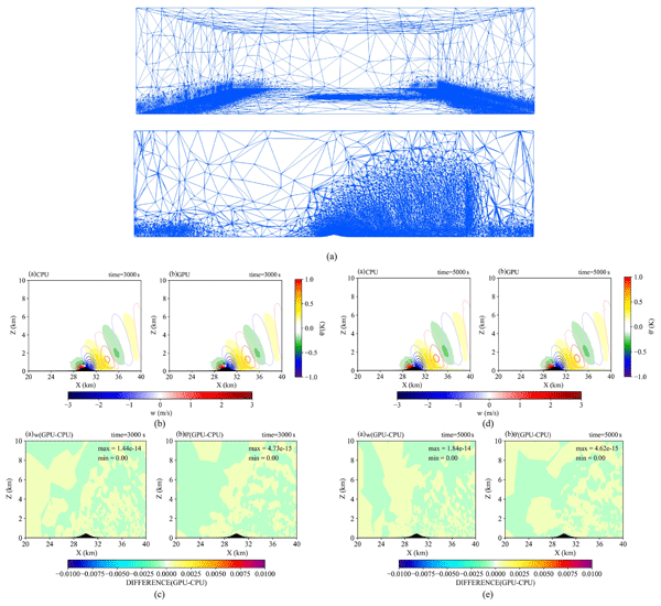
First, to validate the core operators during the non-stationary initial stage, we extract the refined unstructured mesh generated at t = 3000 s from an adaptive run and employ it as a fixed, static grid right from the beginning of the simulation (t=0). Both the CPU and GPU versions simulate the transient phase up to t = 3000 s with the AMR module deactivated. While this static mesh is not dynamically optimized for the early stages, it ensures an identical degree-of-freedom layout from t=0 and completely avoids spatial interpolation errors. Second, to verify long-term stability in the steady-state regime, the simulation is run up to t = 3000 s under the standard CPU-AMR configuration until the wave profile stabilizes. The mesh is then fixed, and both versions advance the physical time independently from t = 3000 s to t = 5000 s. The computational results for both scenarios are presented in Fig. 4. Figure 4a illustrates the 3D wireframe and a 2D cross-sectional slice of the mesh, demonstrating the localized high-resolution refinement adapted to the mountain wave. For the transient fixed-mesh run (Fig. 4b and c), the absolute differences between the CPU and GPU fields at t = 3000 s peak at 1.44 × 10⁻¹⁴ for the vertical velocity (w) and 4.73 × 10⁻¹⁵ for the potential temperature perturbation (θ^′). For the steady-state continuation run (Fig. 4d and e), the differences remain bounded within a similar magnitude at t = 5000 s. These minuscule variations strictly correspond to the double-precision machine epsilon, confirming that the GPU-accelerated operators are fundamentally and mathematically consistent with the original CPU baseline across all simulation phases.

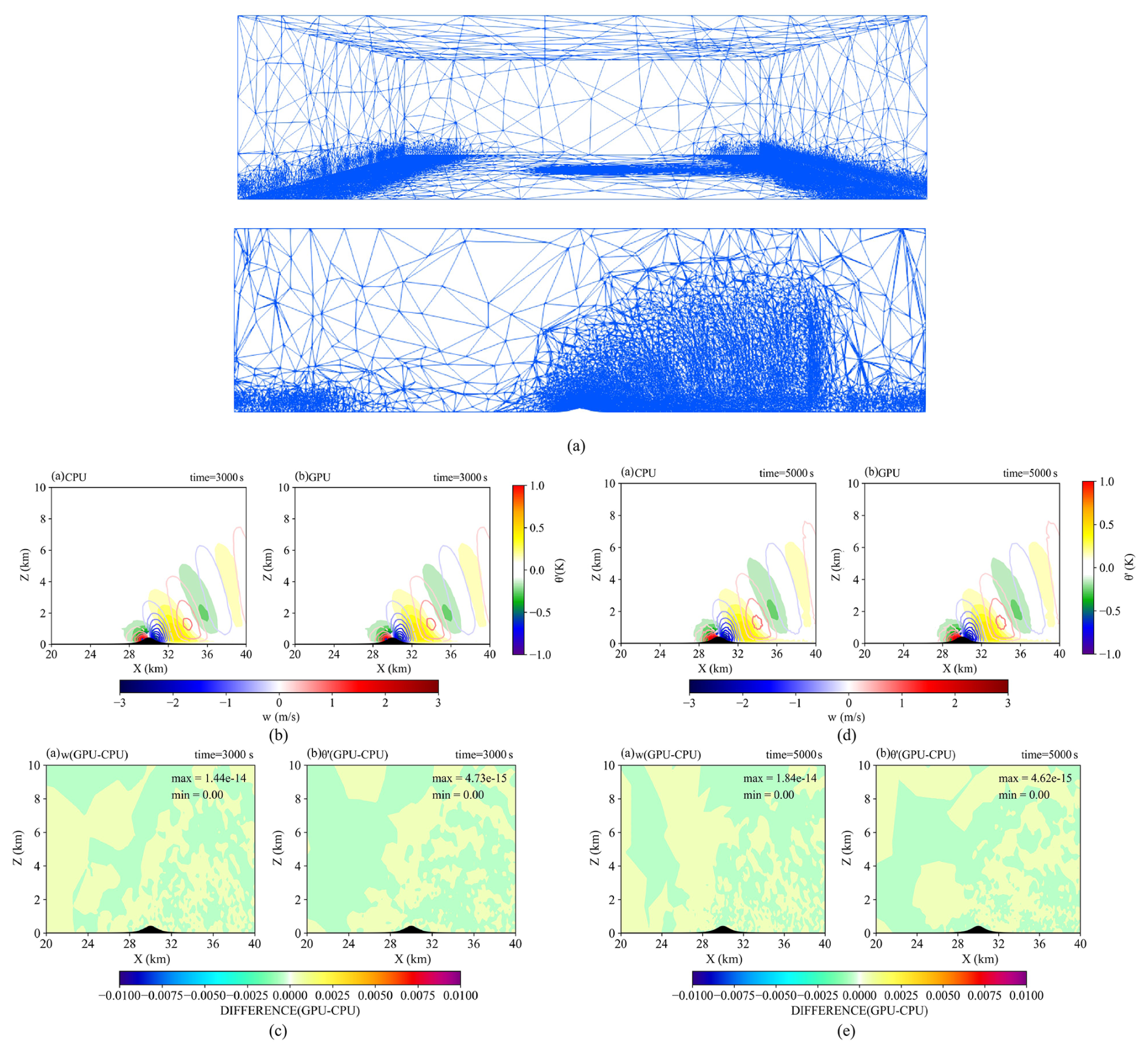
Figure 4 Comparison between the CPU baseline and the GPU-accelerated computation results under fixed-mesh configurations. (a) The unstructured mesh layout visualized via a 3D wireframe and a 2D cross-sectional slice (origin: $(\mathrm{30}\mathrm{000},\mathrm{30}\mathrm{000},-\mathrm{8000})$, normal: $(\mathrm{0},\mathrm{1},\mathrm{0})$) rendered in ParaView; (b) Simulated vertical velocity (w) and potential temperature perturbation (θ^′) fields at t = 3000 s from the transient validation run (simulated continuously from t=0 using the fixed-mesh); (c) Absolute differences between CPU and GPU results at t = 3000 s for the transient fixed-mesh run; (d) Simulated fields at t = 5000 s from the steady-state stability validation run (advanced from t = 3000 s on the fixed-mesh); (e) Absolute differences between CPU and GPU results at t = 5000 s for the steady-state stability run.

5.3 Results and discussion of performance optimization

5.3.1 GPU element-wise computation performance

In unstructured meshes, element node values are typically stored non-contiguously in memory. Thus, the performance of element-wise computation is primarily limited by memory access efficiency. While CPUs incur high memory overhead for non-contiguous access, GPUs leverage high bandwidth and massive thread parallelism to alleviate this bottleneck. Table 3 compares GPU and CPU performance in scalar, vector, and tensor data access. Specifically, functions such as ele_val_scalar serve as data-gathering routines that collect scattered node-based field values from global arrays into contiguous element-local arrays for each element prior to numerical integration. The results demonstrate the GPU's efficiency in accelerating these heavily memory-bound “gather” operations. This is primarily because arrays storing scalar fields have a simpler, lower-dimensional layout, facilitating GPUs to completely leverage high-bandwidth access. All the performance profiling data were collected with the mesh in the Mountainwave3D simulation, in which the number of mesh nodes and elements are 103 635 and 554 394, respectively.

Table 3 GPU Performance of GPU parallel element data access (Mesh: 103 635 nodes, 554 394 elements; timings are averaged over 1000 invocations).

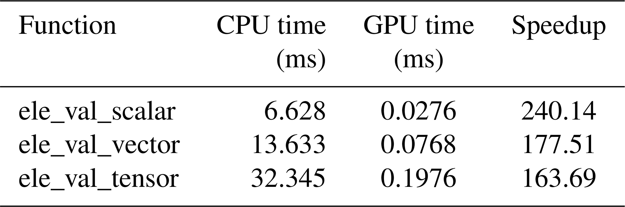
Table 4 GPU kernel performance in element-wise computation (Mesh: 103 635 nodes, 554 394 elements).

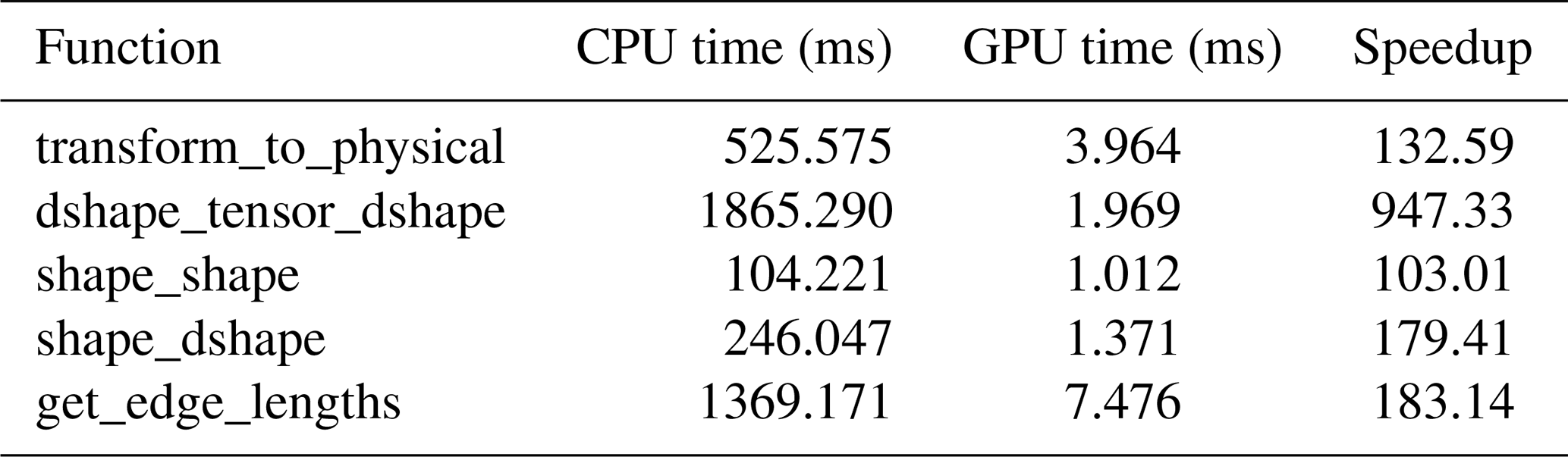
Furthermore, Table 4 presents the GPU performance of numerous core functions in Fluidity-Atmosphere (coordinate transformation, integration, and auxiliary routines). Results indicate that parallelizing dense element-wise computations on GPUs significantly accelerates the performance. All listed functions achieved more than 103× speedups compared with CPU versions. These functions are computationally intensive, involving repeated local linear system and eigenvalue/eigenvector solves for each element in single-core CPU execution. In contrast, the GPU can execute such highly independent tasks concurrently across thousands of threads, comprehensively leveraging parallelism.

Table 5 Performance of dshape_tensor_dshape with optimizations (Mesh: 554 394 elements).

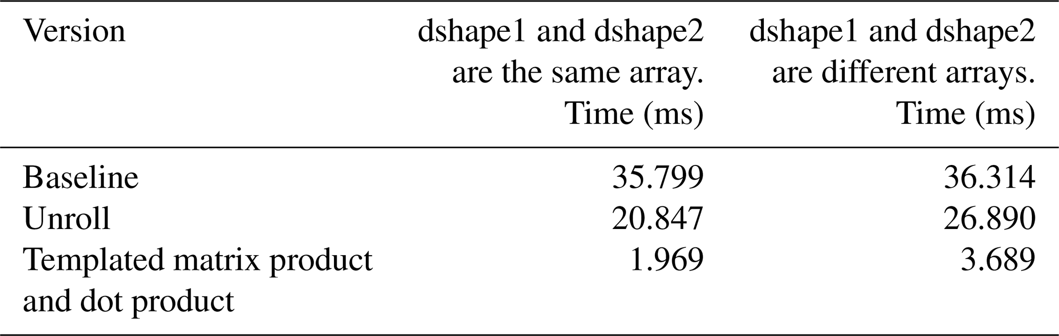
To analyse the effects of GPU-oriented optimizations, we take the dshape_tensor_dshape function as an example. This function is a hotspot in finite-element computation, involving frequent access to gradients of shape functions at Gauss points and dense matrix multiplications/dot products. Table 5 shows performance enhancement due to loop unrolling and optimization via the use of template functions. Notably, Fluidity-Atmosphere typically calls this routine with identical dshape1 and dshape2 arrays. However, for generality we also tested cases with two different dshape1 and dshape2 arrays. While the same array case performs better, both scenarios show consistent performance gains.

Nsight Compute profiling further indicates that templated matrix product and dot product increased memory throughput from 70 % to 82.35 %, slightly improved compute throughput, and enhanced L1 cache hit rates. SASS code inspection revealed that baseline __device__ functions were only locally reordered, thereby limiting the performance. After templating, the compiler applied deeper optimizations, interleaving SASS instructions between __device__ and __global__ functions, yielding significant performance enhancements.

These results confirm that GPU parallelization achieves order-of-magnitude acceleration in element-wise computations, while targeted optimizations further unlock the hardware potential.

5.3.2 Performance of global matrix assembly optimization

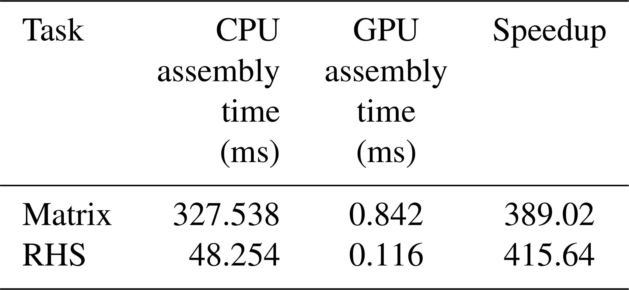
Table 6 shows assembly performance for the advection-diffusion matrix (Temperature) and the right-hand sides. Compared with CPU execution, GPU parallel assembly achieved speedups of up to 389.02× and 415.64×, respectively, highlighting the advantages of massive threading and ultra-high device memory bandwidth. Compared with existing GPU studies on sparse matrix assembly, a substantially higher acceleration is achieved in the proposed method, demonstrating the superior performance of our kernel designs and data structures.

Table 6 Global matrix assembly performance (Mesh: 103 635 nodes, 554 394 elements).

Regarding the parallel assembly, it is worth noting that multiple elements inevitably share nodes in unstructured meshes, which can theoretically introduce memory contention when using atomic operations. To address this, we evaluated alternative algorithms that avoid atomic operations. While this contention-free approach further reduced the sparse matrix update time (e.g., from approximately 5 to 3 ms in specific test stages), it required an explicit mesh preprocessing step. This preprocessing consumed several seconds, introducing an overhead that far outweighed the modest kernel-level savings. Therefore, the direct atomic operation algorithm was selected for its simplicity and overall efficiency. This design choice is further supported by recent evaluations of unstructured-grid CFD applications on GPUs, which demonstrate that NVIDIA V100 and A100 architectures inherently deliver exceptional performance on kernels dominated by double-precision atomic updates, often outperforming complex register-based aggregation or data restructuring methods (Stone et al., 2021).

5.3.3 Hardware utilization and bottleneck analysis

To further comprehend the GPU execution efficiency, we analyzed the hardware utilization of our core kernels using NVIDIA Nsight Compute. The theoretical FP64 peak performance of the A100 GPU is 9.7 TFLOP s⁻¹. However, in unstructured FEM frameworks, performance is predominantly bounded by memory bandwidth rather than compute capabilities.

For the element-wise integration kernel dshape_tensor_dshape, the Compute (SM) Throughput reached approximately 8.50 % of the theoretical peak. While this kernel involves intensive small-matrix multiplications, its arithmetic intensity is inherently constrained by the necessity to fetch scattered nodal variables and coordinates from the global memory for each element. This is strongly evidenced by its Memory Throughput, which achieved an outstanding 90.44 % of the device's peak memory bandwidth, indicating that the kernel is optimally saturating the hardware's memory subsystem.

Similarly, the global matrix assembly assemble_csr_matrix and RHS construction rhs_addto_kernel kernels are archetypal memory-bound operations. Their Compute Throughputs are limited to 7.93 % and 18.29 %, respectively, primarily because they execute sparse floating-point operations (such as atomic additions) amidst heavy indirect memory accesses. Instead, their execution efficiency is profoundly reflected in their Memory Throughputs, which achieved 79.48 % and 82.98 %, respectively. Given the highly irregular access patterns dictated by unstructured mesh connectivity (e.g., indirect addressing via row_pointers and ndglno), maintaining such high memory bandwidth utilization demonstrates that our data layout and atomic-based assembly strategies effectively saturate the hardware limits for these memory-intensive workloads.

Table 7 Pinned vs non-pinned memory transfer performance.

5.3.4 CPU-GPU data transfer and overlap with computation

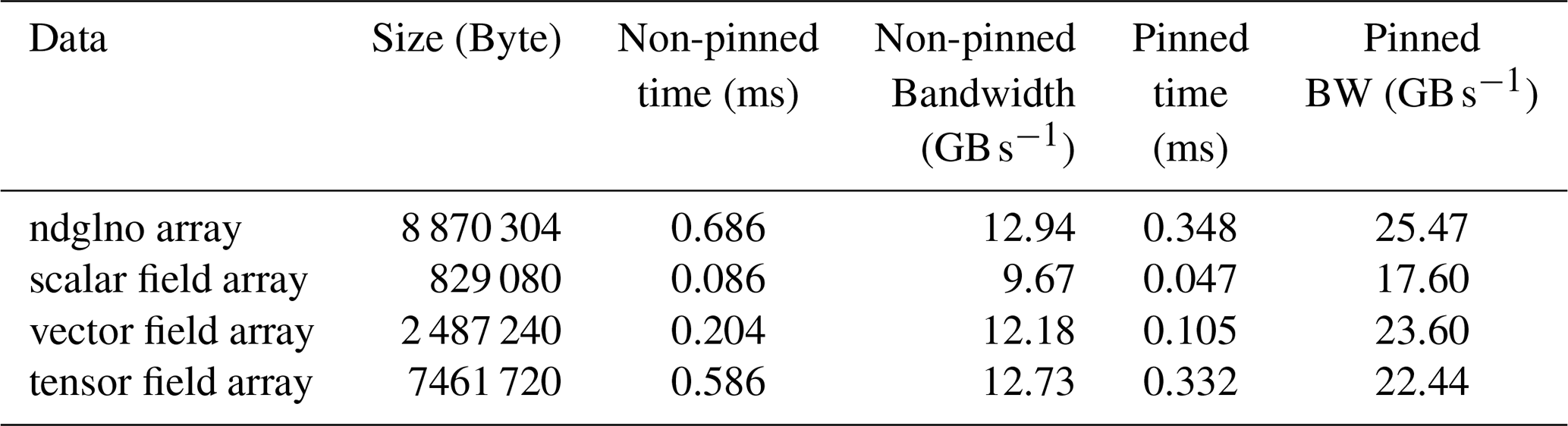
In hotspot acceleration, CPU-GPU data transfer is another critical performance factor. In our system, CPU and GPU are connected via PCIe 4.0 × 16, with a bidirectional bandwidth of 32 GB s⁻¹. When the CPU has pinned memory, transfer bandwidth utilization is significantly higher than that with pageable memory. During Fluidity-Atmosphere computation, the type of data transferred frequently between the CPU and GPU includes scalar, vector, and tensor field arrays, the element-node connectivity array (ndglno), as well as the fully assembled global sparse matrix arrays returning from the GPU device memory to the host for PETSc solvers. Table 7 compares pinned and non-pinned transfer performance, displaying an evidently superior bandwidth with pinned memory.

In addition, CUDA provides stream concurrency and asynchronous APIs such as cudaMemcpyAsync, facilitating simultaneous data transfer and kernel execution. The transform_to_physical kernels can run concurrently with transfers of subsequent physical field data. The transfer-computation overlap effectively mitigates communication bottlenecks and further leverages HPC system performance.

Table 8 GPU acceleration performance of major modules.

5.3.5 Performance of functional modules

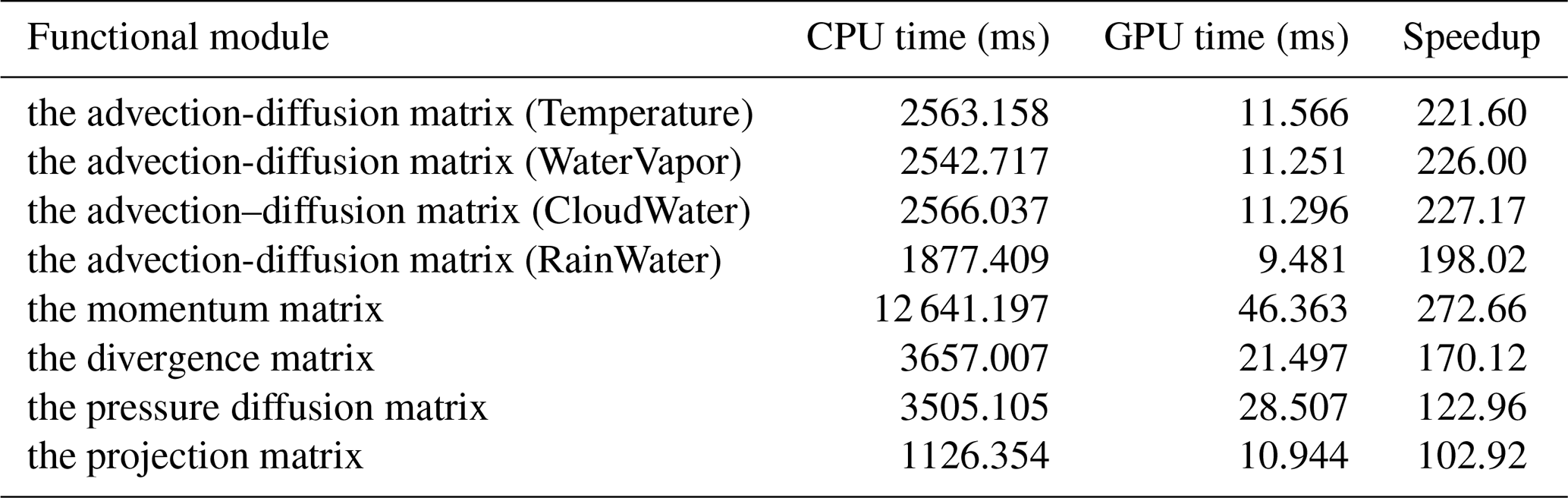
After embedding GPU-accelerated element-wise computation and global assembly strategies into Fluidity-Atmosphere, we evaluated the overall performance at three levels: module, single timestep, and multi-process parallelism. In the restarting Mountainwave3D simulation, the pressure diffusion matrix was calculated only once, and the others were the average times of simulation timesteps which ranges from 3000 to 5000 s. Table 8 summarizes performance across major functional modules.

As the global sparse linear solver was not GPU-parallelized, the overall acceleration for the single-process execution remained limited. However, Fluidity-Atmosphere already supports MPI, enabling MPI+GPU hybrid execution for maximal performance. Table 9 compares the one timestep execution performance using different numbers of CPU cores (MPI processes) and GPU-enabled configurations.

Table 9 The performance of GPU accelerated Fluidity-Atmosphere.

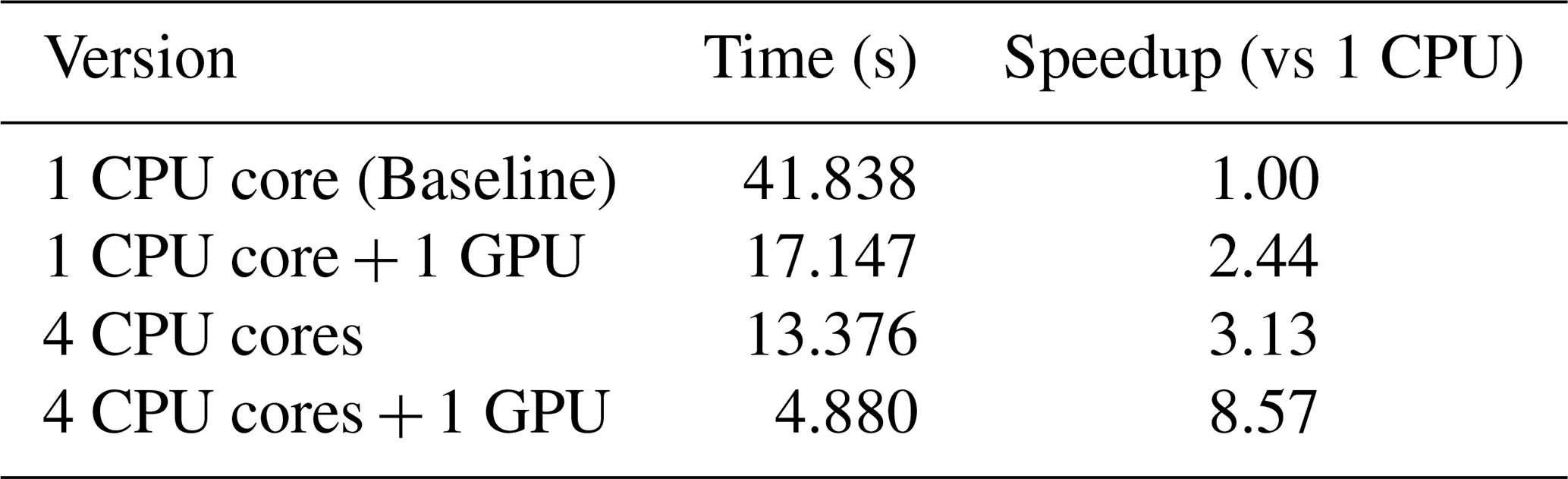
The results show that GPU acceleration achieved a 2.44× speedup for single-process execution. With 4 MPI processes (each handling approximately 25 000 nodes and 140 000 elements), the hybrid MPI + GPU version achieved 8.57× speedup compared with single CPU core execution. Table 9 presents the average times of simulation timesteps which ranges from 3000 to 5000 s.

Table 10 Comparison of computational performance and runtime distribution across different configurations (Unit: Time in seconds, Percentage of total timestep).

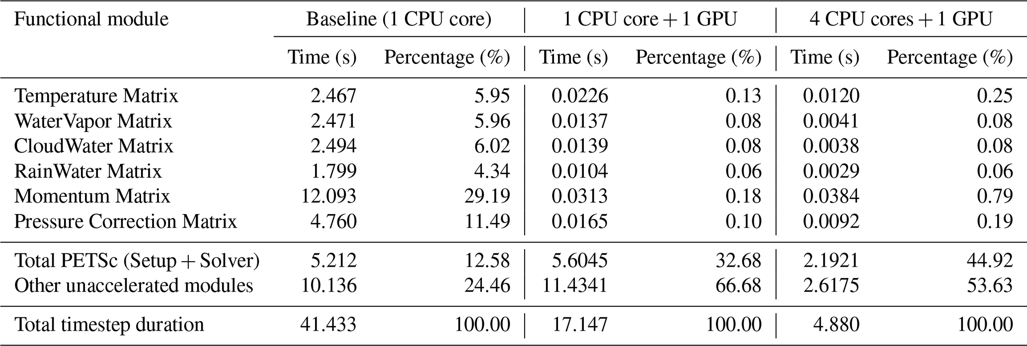
Notably, the 4 CPU cores + 1 GPU configuration achieves an 8.57× speedup, which is more than triple the speedup of the 1 CPU core + 1 GPU configuration (2.44×). This synergistic effect is attributed to two factors: first, the domain decomposition in multi-process execution allows the remaining CPU-bound linear solvers (PETSc) to benefit from improved cache locality on smaller sub-domains; second, multiple MPI processes can concurrently issue kernels to the GPU via CUDA streams, leading to higher hardware occupancy on the NVIDIA A100. As detailed in Table 10, this configuration effectively addresses the “bottleneck shift” dictated by Amdahl's Law. In the 1 CPU core + 1 GPU setup, GPU matrix assembly is compressed to less than 1 % of the total time, leaving the PETSc solver and other unaccelerated modules as the dominant bottlenecks. However, by leveraging 4 MPI processes, the absolute execution time of the PETSc solver is dramatically reduced from 5.60 to 2.19 s, and the time for other unaccelerated modules drops from 11.43 to 2.62 s. This multi-core mitigation of the remaining CPU bottlenecks, combined with sustained GPU efficiency, strictly validates the 8.57× overall performance gain.

6 Conclusions

This study focuses on the unstructured-mesh finite-element atmospheric model named Fluidity-Atmosphere, thereby addressing the computational bottlenecks in element-wise computations and matrix assembly. Leveraging the architectural features of the NVIDIA A100 GPU and the CUDA programming model, we designed and implemented GPU-oriented parallel optimization strategies. The proposed high-performance GPU kernels substantially enhanced the computational efficiency while solving the momentum equations, advection equations, and stabilization term construction, thereby accelerating critical processes in atmospheric numerical simulations. For element-wise computations, template-based kernel design and deep optimizations achieved speedups ranging from tens to several hundred times. With asynchronous data transfer and MPI parallelization, an overall acceleration that is 8.57 times greater than that of the CPU version was achieved using four processes while ensuring correctness and stability in multi-time step simulations. The proposed parallelization methods substantially enhance the performance of atmospheric models on heterogeneous systems, remarkably extending the support for high-performance implementations of unstructured-mesh models. Future work will focus on further overcoming performance bottlenecks in the overall simulation, particularly by migrating the sparse linear solver (which is still CPU-dependent) to GPUs, thereby facilitating end-to-end acceleration.

Appendix A: Code

template<int T_M>
__device__ double dot_product_t(double*__restrict__ a,
double* __restrict__ b){
    double r=0.0;
    #pragma unroll
    for(int i=0;i<T_M;i++){
        r += a[i]*b[i];
    }
    return r;
}

// T_M, T_N, T_K: Matrix dimensions for generic small matrix multiplication
template<int T_M, int T_N, int T_K>
__device__ void __forceinline__  matmul_t(const double* a, const double* b, double* C){
    for (int mi = 0; mi < T_M; ++mi) {
        for (int ki = 0; ki < T_K; ++ki) {
            #pragma unroll
            for (int ni = 0; ni < T_N; ++ni) {
               // Column-major layout stride; efficient due to thread-local
               // register/L1 caching
               C[ni* T_M + mi] +=  a[ki * T_M + mi] * b[T_K * ni + ki];
            }
        }
    }
}

// T_dim: Spatial dimension (e.g., 3 for 3D)
// T_loc1, T_loc2: Number of local nodes per element
// T_ngi: Number of Gauss integration points
template<int T_dim, int T_loc1, int T_loc2, int T_ngi>
__device__ void dshape_tensor_dshape_unroll_t(const double *dshape1,
const double *tensor,const double *dshape2, const double *detwei, double *r){
    double tmp[T_dim]={0.0},mat_mul[T_dim]={0.0},dotproduct=0.0;
    for(int gi=0; gi< T_ngi;++gi){
        double gidetwei=detwei[gi];
        for(int iloc=0;iloc<T_loc1;iloc++){
            #pragma unroll
            for(int n=0;n<T_dim;++n){
                tmp[n]=dshape1[n*T_ngi*T_loc1+gi*T_loc1+iloc];
                mat_mul[n] = 0.0;
            }
            // <1,3,3> literals explicitly used to unroll 3D spatial
            // vector-tensor interaction
            matmul_t<1,3,3>(tmp,&tensor[gi*T_dim*T_dim],mat_mul);
            for(int jloc=0;jloc<T_loc2;jloc++){
                #pragma unroll
                for(int n=0;n<T_dim;++n){
                    tmp[n]=dshape2[n*T_ngi*T_loc2+gi*T_loc2+jloc];
                }
                dotproduct = dot_product_t<T_dim>(mat_mul,tmp);
                r[jloc*T_loc1+iloc]=r[jloc*T_loc1+iloc]+dotproduct*gidetwei;
            }
        }
    }
}

Appendix B: Code

template<int T_dim, int T_loc, int T_ngi>
__global__ void assemble_csr_matrix(double *result, double* values,
int *row_pointers, int *col_index, int *ndglno, const int ele_num){
    int element_index = blockIdx.x*blockDim.x + threadIdx.x;
    if(element_index>=ele_num) return;
    int loc1=T_loc;
    int loc2=T_loc;
    int mpos=0,base=0,upper_j=0,upper_pos=0,lower_j=0,lower_pos=0,
        this_pos=0,this_j=0;
    int inode[T_loc]={0};
    int j=0;
    double *element_result=result + element_index *T_loc * T_loc;
    int *row=nullptr;
    int iloc=0, jloc=0,  n=0;
    //ndglno stores the connectivity for neighbouring elements.
    for(int i = 0; i < T_loc; ++i){
      inode[i]= ndglno[element_index * loc1 + i];
    }
    for(iloc=0;iloc<loc1;iloc++){
        //the index in Fluidity-Atmosphere Fortran code is from 1.
        base = row_pointers[inode[iloc]-1]-1;
        n = row_pointers[inode[iloc]] -1 - base;
        for(jloc=0;jloc<loc2;jloc++){
            if(element_result[jloc*loc1+iloc]==0)continue;
            row = col_index+base;
            upper_pos=n-1;
            upper_j=row[n-1]-1;
            lower_pos=0;
            lower_j=row[0]-1;
            mpos=-2;
            j = inode[jloc]-1;
            if (upper_j<j){
                mpos=-1;
            }else if (upper_j==j){
                mpos=upper_pos+base;
            }else if (lower_j>j){
                mpos=-1;
            }else if(lower_j==j){
                mpos=lower_pos+base;
            }

            while(((upper_pos-lower_pos)>1)&&(mpos==-2)){
                this_pos=(upper_pos+lower_pos)/2;
                this_j=row[this_pos]-1;
                if(this_j == (inode[jloc]-1)){
                    mpos=this_pos+base;
                }
                else if(this_j > (inode[jloc]-1)){
                    upper_j=this_j;
                    upper_pos=this_pos;
                }
                else{
                    lower_j=this_j;
                    lower_pos=this_pos;
                }
            }
            if(mpos<0){
            }else{
                atomicAdd(values+mpos,element_result[jloc*loc1+iloc]);
            }
        }
    }
}

Appendix C: Code

template<int T_loc>
__global__ void rhs_addto_kernel(GpuScalarField *field, const int ele_num,
double *gpu_ele_val){
    int  element_index = blockDim.x * blockIdx.x + threadIdx.x;
    if(element_index >=ele_num) return;
    //element_index will be used to find the node indexes starting from 1.
    element_index = element_index + 1;
    int nodes[T_loc];
    //get the node indexes of current element.
    gpu_ele_nodes_scalar(*field, element_index,nodes);
    double *ptr = gpu_ele_val + (element_index -1)*T_loc;
    #pragma unroll
    for(int i = 0; i < T_loc;++i){
        atomicAdd(&(*field).val[(nodes[i] -1)],*(ptr+i));
    }
}