Enhancing air–sea CO₂ exchange and modulating seawater carbonate–pH dynamics: the role of wave effect mechanisms in the POP2–waves coupled model

In this study, a wave module is online-coupled into the Parallel Ocean Program version 2 (POP2) within the CESM1.2.2 framework (hereafter POP2–waves). Unlike empirical data analyses of observation-based products and offline-forced ocean models that treat wave-induced gas transfer velocity and the air–sea difference in partial pressure of CO₂ (ΔpCO₂) as decoupled variables, the online-coupled POP2–waves model captures their interactive, ΔpCO₂-mediated negative feedbacks. This setup enables wave properties to dynamically modulate gas transfer velocity and physical mixing through sequential processes. POP2–waves is evaluated alongside a control simulation (B–CTL) against the National Oceanic and Atmospheric Administration (NOAA) CarbonTracker (CT2022) inversion product. The spatial air–sea CO₂ flux in POP2–waves simulation shows generally closer structural agreement with NOAA CT2022 than the control B–CTL, thereby improving performance in most selected regions. Specifically, bubble-mediated transfer accounts for up to 41.3 % of the total flux, consistent with the ∼40 % contribution reported in recent research. Although the inclusion of waves (POP2–waves) enhances regional oceanic CO₂ uptake by 11.8 % and outgassing by 41.6 %, these two processes largely offset each other. Consequently, this dual enhancement results in only a slight 1.8 % increase in the global net ocean CO₂ sink compared to the B–CTL simulation. Globally, air–sea ΔpCO₂ and pH exhibit the strongest positive and negative regression coefficients with the air–sea CO₂ flux, respectively. Regionally, the gas transfer velocity shows a positive (negative) regression coefficient within oceanic CO₂ outgassing (uptake) regions, whereas SST displays the opposite trend.

1 Introduction

The exchange of CO₂ between the air and sea is a crucial component of the global carbon cycle, carrying significant implications for Earth's climate (Bange et al., 2024; Friedlingstein et al., 2022; McKinley et al., 2020; Müller et al., 2023; Shutler et al., 2019). Traditionally, this air–sea exchange is characterized using the bulk formula (e.g., Wanninkhof, 1992, 2014; McKinley et al., 2020; Dong et al., 2022; Fay et al., 2021; Zhou et al., 2023; Heimdal et al., 2024):

$$\begin{array}{}\text{(1)}& F_{{\mathrm{CO}}_{\mathrm{2}}}=k_{\mathrm{w},\mathrm{660}}\cdot k_{\mathrm{0}}\cdot (p{\mathrm{CO}}_{\mathrm{2}}^{\mathrm{w}}-p{\mathrm{CO}}_{\mathrm{2}}^{\mathrm{a}})\cdot (\mathrm{1}-\mathrm{ice})\end{array}$$

where the air–sea CO₂ flux ($F_{{\mathrm{CO}}_{\mathrm{2}}}$, mol m⁻² yr⁻¹) is determined by the gas transfer velocity expressed relative to a Schmidt number of 660 (k_w,660, cm h⁻¹), the difference in partial pressure of CO₂ (ΔpCO₂, µatm) between the seawater and atmosphere (indicated by superscripts “w” and “a”, respectively), and the solubility constant (k₀; mol m⁻³ atm⁻¹), which varies with salinity and temperature (Weiss, 1974). Note that an appropriate scaling factor ($\mathrm{8.76}\times {\mathrm{10}}^{-\mathrm{5}}$) is implicitly required to convert the dimensions of k_w,660 and ΔpCO₂ into the final flux unit (mol m⁻² yr⁻¹). The sign of air–sea CO₂ flux is determined by ΔpCO₂, where a positive air–sea CO₂ flux indicates ocean outgassing to the atmosphere. Additionally, the calculated fluxes are weighted by the ice-free fraction (1−ice), where “ice” represents the sea ice fraction. The estimation of bulk air–sea CO₂ fluxes using the gas transfer velocity is typically based on the Wanninkhof (1992) formulation:

$$\begin{array}{}\text{(2)}& k_{\mathrm{w},\mathrm{660}}=\mathrm{0.31}<U_{\mathrm{10}}^{\mathrm{2}}>(Sc/\mathrm{660}{)}^{-\mathrm{0.5}}\end{array}$$

where $<U_{\mathrm{10}}^{\mathrm{2}}>$ represents the squared neutral mean wind speed at 10 m above the surface (m s⁻¹), and Sc denotes the Schmidt number. The flux estimate error can reach as high as 34 % due to model limitations and uncertainties surrounding bulk parameters (Signorini and McClain, 2009). Furthermore, substantial uncertainties persist in air–sea CO₂ flux estimates, primarily stemming from an incomplete understanding of the spatiotemporal variability in the governing mechanisms (Shutler et al., 2019).

Some studies have highlighted that estimating air–sea CO₂ fluxes involves complexities well beyond neutral wind speed and solubility factors. Monahan and Spillane (1984) previously regarded whitecaps as “low impedance vents” that effectively “shorten” the water-side transfer resistance. Without wave breaking, air–sea CO₂ exchange occurs via mass transport, which under non-turbulent conditions is governed by molecular diffusion; wave breaking then acts as a transitional process from laminar to turbulent flow (Deike, 2022). Furthermore, bubbles provide additional surface area for gas transfer; as they rise through the aqueous mass boundary layer and burst at the sea surface, they significantly enhance near-surface turbulence (Soloviev and Lukas, 2010; Bell et al., 2017; Deike and Melville, 2018; Krall et al., 2019; Czerski et al., 2022). Gutiérrez-Loza et al. (2022) pointed out that during high and intermediate wind speeds (above 6–8 m s⁻¹), enhanced air–sea CO₂ exchange is primarily driven by wave-breaking dynamics and bubble mediation, which occur alongside the generation of sea spray droplets that contribute to atmospheric cloud condensation nucleation. Conversely, under low wind conditions (below 6 m s⁻¹), water-side convection becomes the dominant control mechanism. Beyond these calm periods, the critical role of breaking waves and bubble injection mechanisms in facilitating CO₂ transfer has been widely corroborated (e.g., Andreas et al., 2016; Brumer et al., 2017; Blomquist et al., 2017; Reichl and Deike, 2020; Li et al., 2023; Zhou et al., 2023; Rustogi et al., 2025). Specifically, Deike and Melville (2018) demonstrated that the bubble-mediated contribution to CO₂ transfer exceeds 40 % at a neutral 10 m wind speed (U₁₀)≥10 m s⁻¹, becomes dominant at U₁₀≥15 m s⁻¹, and reaches 60 % at 20 m s⁻¹.

Monitoring sea surface CO₂ is crucial for understanding Earth system dynamics, as climate change has begun to impact the ocean's carbon uptake capacity (Behncke et al., 2024). However, air–sea CO₂ flux estimates derived from products based on the partial pressure of CO₂ (pCO₂) often suffer from significant uncertainties, stemming primarily from the empirical parameterization of the gas transfer velocity (e.g., Williams et al., 2017; Gray et al., 2018; Coggins et al., 2023; Behncke et al., 2024; Fay et al., 2024; Yang et al., 2024). To resolve this issue and independently constrain k_w,660, direct flux measurements using the eddy covariance (EC) method are widely utilized as a benchmark (Dong et al., 2021). By directly acquiring the turbulent flux $F_{{\mathrm{CO}}_{\mathrm{2}}}$ via the EC method and pairing it with simultaneous measurements of ΔpCO₂, researchers can inversely calculate the gas transfer velocity ($k_{\mathrm{w},\mathrm{660}}=F_{{\mathrm{CO}}_{\mathrm{2}}}/(k_{\mathrm{0}}\times \mathrm{\Delta }p$CO₂)). This approach provides a direct observational constraint to evaluate and calibrate these observation-based products under complex marine conditions. However, obtaining reliable direct fluxes from shipborne EC setups presents its own instrumental challenges. Marine EC measurements are generally conducted using either open- or closed-path infrared gas analyzers. A closed-path analyzer (e.g., LI-7000, LI-COR) operates with an enclosed measurement chamber (Sutton et al., 2014, 2021; Bakker et al., 2016; Sabine et al., 2020; Akhand et al., 2021; Wu and Qi, 2023), whereas open-path analyzers (e.g., LI-7500, LI-COR) measure infrared absorption directly in ambient air (Edson et al., 2011; Tokoro et al., 2014; Bell et al., 2017; Dong et al., 2021; Van Dam et al., 2021). While both configurations are inherently susceptible to H₂O cross-sensitivity, each system possesses distinct advantages and systematic limitations (Honkanen et al., 2018). Evaluating and constraining global Earth system models (ESMs) against direct, long-term observations of air–sea CO₂ flux remains challenging due to the severe scarcity of continuous field measurements. Consequently, alternative validation datasets are typically derived by upscaling sparse in situ pCO₂ observations through a combination of statistical interpolation, machine learning, atmospheric inversion, and climatological averaging to construct long-term, gridded flux products.

Although several recent studies have estimated the air–sea CO₂ flux using Eq. (1), current parameterizations in oceanic and atmospheric models still rely exclusively on neutral wind speed (Long et al., 2013; Moore et al., 2013; Couldrey et al., 2016; Jin et al., 2017; Lovenduski et al., 2019; Ziehn et al., 2020; Chikamoto and DiNezio, 2021). Similarly, surface ocean observation-based products typically calculate those fluxes using standard parameterizations (Wanninkhof, 1992, 2014; Fay et al., 2021). Importantly, the persistent uptake of anthropogenic CO₂ is lowering seawater pH and altering the carbonate system in nonlinear ways, further reducing the oceans' capacity to absorb additional CO₂ (Moore et al., 2013). The mechanisms by which breaking waves and bubble injection enhance total gas transfer velocity have been investigated primarily through empirical analyses of observation-based products (e.g., Andreas et al., 2016; Blomquist et al., 2017; Reichl and Deike, 2020; Zhou et al., 2023). Rustogi et al. (2025) employed a fully coupled ocean-biogeochemistry modeling system based on the MOM6 ocean circulation model and the COBALTv2 biogeochemical module. Utilizing this framework, they simulated ocean dynamics, temperature, and carbon cycling processes – including dissolved inorganic carbon (DIC) and pCO₂ – while explicitly accounting for wave effects on air–sea CO₂ exchange. Furthermore, they identified a nonlinear pCO₂ feedback mechanism within the coupled ocean-carbon system that regulates air–sea CO₂ flux. However, their configuration relies on ocean and biogeochemical modules that are strictly forced by offline atmospheric reanalysis and wave model outputs. This decoupled or unidirectional forcing approach is limited in capturing high-frequency, transient air–sea interactions (e.g., rapid wind shifts or wave breaking dynamics) that significantly modulate gas exchange. In contrast, our study introduces an online coupling framework that integrates wave effects directly into the flux simulation interface at each model time step. This online approach provides a critical advantage: it enables real-time, interactive feedback between wave dynamics and the seawater carbonate system, thereby capturing the nonlinear high-frequency physical controls on the air–sea CO₂ flux that offline-forced systems typically miss.

In this study, we investigate how breaking waves and bubble injection mechanisms influence air–sea CO₂ flux and the ocean's buffering capacity. Specifically, we examine the biogeochemical responses driven by these physical mechanisms within the seawater carbonate–pH system. To achieve this, we utilize the Parallel Ocean Program version 2 (POP2; Smith et al., 2010) of the Community Earth System Model version 1.2.2 (CESM1.2.2; Hurrell et al., 2013) online-coupled with the wave module (Mellor et al., 2008) of the Princeton Ocean Model (POM; Blumberg and Mellor, 1987). The coupled configuration is referred to as the POP2–waves model.

The structure of this paper is organized as follows. Section 2 introduces the model, data, methodology, and experiments employed in this study, and defines twelve key regions of high air–sea CO₂ flux variability identified by the NOAA CarbonTracker data assimilation system (CT2022; Jacobson et al., 2023) to validate the model simulation. Section 3 evaluates the performance of the POP2–waves coupled model in simulating air–sea CO₂ flux and its interaction with the carbonate–pH system over the Western Pacific (WP; 160–180° E, 35–40° N) and the Equatorial Pacific (EP; 230–250° E, 0–5° S) regions. Section 4 compares the carbonate–pH dynamics of POP2–waves and B–CTL, examines the primary drivers of air–sea CO₂ exchange, and evaluates the uncertainties arising from the absence of a ΔpCO₂-driven negative feedback. Finally, Sect. 5 presents the conclusions.

2 Data, model experiments, and methodology

2.1 Description of the model framework and experiments

In this study, we investigate the role of waves and bubble mechanisms in modulating the ocean's biogeochemical response by comparing the control simulation (B–CTL) with the coupled POP2–waves model within the CESM1.2.2 framework (Fig. 1). The CESM simulation was conducted using a fully coupled component set over a 30-year period, with well-mixed greenhouse gases (CO₂, CH₄, N₂O, etc.), ozone, and aerosols fixed to year-2000 values (the B_2000_CAM5 compset). The framework features a horizontal resolution of 1.9°×2.5° for both the Community Atmosphere Model 5.3 (CAM5.3) and the Community Land Model version 4 (CLM4). In contrast, the ocean component (POP2; configured with 60 vertical layers) and the prognostic Los Alamos Sea Ice Model (CICE) share a nominal 1° horizontal resolution. State fields and fluxes are exchanged across these differing grids via the coupler (CPL) (Hurrell et al., 2013). POP2 is forced by CAM5.3 through CPL via four primary fields: (1) momentum fluxes (zonal and meridional wind stress and friction velocity), (2) heat fluxes (net shortwave radiation, sensible heat flux, longwave radiation, and heat flux from snow/ice melt), (3) freshwater fluxes (precipitation, evaporation, river runoff, and ice melt), and (4) surface winds (10 m zonal and meridional wind speeds). Furthermore, POP2 interacts with the Biogeochemical Elemental Cycling (BEC; Moore et al., 2013) module to regulate carbonate chemistry and air–sea CO₂ fluxes. This interaction is mediated via ocean dynamics (currents and sea surface height), the K-profile vertical mixing, and tracer transport, with wave-induced processes providing additional physical constraints. Within the BEC module, variations in DIC and nutrients (NO₃, PO₄, and Fe) are primarily controlled by biological processes: photosynthesis consumes DIC and nutrients, whereas respiration and remineralization return organic carbon to the DIC pool. Together with the wave module, these biogeochemical and physical processes jointly regulate the carbon cycle.

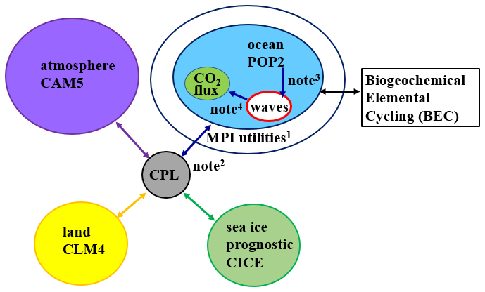
Figure 1 Architecture diagram for POP2–waves experiment in CESM1.2.2 framework, all components adhere to the CESM1.2.2 framework, except for certain parts of the ocean component. The model components including components for the atmosphere [Community Atmosphere Model version 5 (CAM5)], land [Community Land Model version 4 (CLM4)], ocean [Parallel Ocean Program, version 2 (POP2)], along with its associated modules – the waves module (waves) and the Biogeochemical Elemental Cycling (BEC) module – sea ice [prognostic Los Alamos Sea Ice Model (CICE)], and the coupler (CPL). Note: (1) The wave-module variables are communicated between neighboring blocks via MPI, including zonal and meridional 10 m winds, wave radiation stress, subsurface momentum, and wave radiation and energy densities. (2) To transfer variables such as zonal and meridional 10 m winds and friction velocity (including sea surface and ice fraction) from the CPL to POP2. (3) The wave module receives variables from POP2, including the interpolation of depth-varying currents from z-coordinates (60 levels) to the wave module's vertical sigma coordinates (21 levels), along with ocean grid information in the x, y, and z directions. (4) The wave module outputs significant wave height and friction velocity from the CPL for calculating the bubble-mediated gas transfer velocity in Eq. (3).

The control simulation (B–CTL), which served as the baseline for air–sea CO₂ flux and seawater acidification, utilized Eq. (1) with the gas transfer velocity parameterization from Wanninkhof (1992) (Eq. 2). Both the B–CTL and POP2–waves experiments were integrated under a present-day scenario (starting from the year 2000) to estimate air–sea CO₂ flux and pH variations. This experimental design allows us to isolate the impact of wave effects on carbonate chemistry and directly compare our results with the NOAA CT2022 data assimilation system. For the POP2–waves experiment, the wave module (Mellor et al., 2008) from the POM was online-coupled with POP2. This configuration incorporated bubble-mediated gas transfer – computed from a mechanistic model for air bubble entrainment at the breaking-wave scale (Deike and Melville, 2018) – and was integrated with the POP2 marine biogeochemistry module.

Specifically, the POP2–waves experiment adopts the advanced parameterization framework expanded by Reichl and Deike (2020), and Deike (2022). In this framework, both the non-bubble and bubble-mediated gas transfer velocity are explicitly resolved as a function of the ocean surface friction velocity (u^*, m s⁻¹) and significant wave height (H_s, m). This parameterization effectively captures the main wave effect, as well as solubility and diffusivity. To standardize the formulation for CO₂, the total gas transfer velocity is expressed relative to a Schmidt number of 660. Following Deike and Melville (2018), it is calculated as the sum of the non-bubble (k_wNB,660) and bubble (k_wB,660) components:

$$\begin{array}{}\text{(3)}& \begin{array}{rl}{k}_{\mathrm{w},\mathrm{660}}& =k_{\mathrm{wNB},\mathrm{660}}+k_{\mathrm{wB},\mathrm{660}}=A_{\mathrm{NB}}{u}^{*}{\left({\displaystyle \frac{Sc}{\mathrm{660}}}\right)}^{-\mathrm{1}/\mathrm{2}}\\ & +{\displaystyle \frac{A_{\mathrm{B}}}{k_{\mathrm{0}}R{T}_{\mathrm{0}}}}(u^{*}{)}^{\mathrm{5}/\mathrm{3}}{\left(g{H}_{\mathrm{s}}\right)}^{\mathrm{2}/\mathrm{3}}{\left({\displaystyle \frac{Sc}{\mathrm{660}}}\right)}^{-\mathrm{1}/\mathrm{2}}\end{array}\end{array}$$

where A_NB is an empirical, nondimensional coefficient set to $\mathrm{1.55}\times {\mathrm{10}}^{-\mathrm{4}}$, A_B is a dimensional fitting coefficient ($\mathrm{1.2}\times {\mathrm{10}}^{-\mathrm{5}}$ s² m⁻²), R is the ideal gas constant (0.082 L atm mol⁻¹ K⁻¹), T₀ is the sea surface temperature (SST, in K), and g is gravitational acceleration (9.806 m s⁻²). Section 3.3 examines the relative contributions of the non-bubble and bubble components in simulating the air–sea CO₂ flux.

The marine carbonic acid system is a nonlinear, coupled system governed by CO₂ dissolution equilibrium, $\left({\mathrm{CO}}_{\mathrm{2}\left(\mathrm{aq}\right)}+{\mathrm{H}}_{\mathrm{2}}\mathrm{O}\stackrel{K_{\mathrm{H}}}{⟷}{\mathrm{H}}_{\mathrm{2}}{\mathrm{CO}}_{\mathrm{3}\left(\mathrm{aq}\right)}\right)$, where the Henry's constant (K_H) for CO₂ in water at 25 °C is approximately $\mathrm{3.4}\times {\mathrm{10}}^{-\mathrm{2}}$ (m atm⁻¹), two-step dissociation reactions, and the conservation of the total dissolved inorganic carbon (DIC) and total alkalinity (TA), ultimately determining pH and the distribution of carbonate species. Carbonic acid (H₂CO₃) has two hydrogen ions and dissociates in two steps:

$$\begin{array}{}\text{(4)}& {\displaystyle }{\mathrm{H}}_{\mathrm{2}}{\mathrm{CO}}_{\mathrm{3}}\stackrel{K_{\mathrm{a}\mathrm{1}}}{⟷}{\mathrm{H}}^{+}+{\mathrm{HCO}}_{\mathrm{3}}^{-}{K}_{\mathrm{a}\mathrm{1}}=\mathrm{4.4}\times {\mathrm{10}}^{-\mathrm{7}}\text{(5)}& {\displaystyle }{\mathrm{HCO}}_{\mathrm{3}}^{-}\stackrel{K_{\mathrm{a}\mathrm{2}}}{⟷}{\mathrm{H}}^{+}+{\mathrm{CO}}_{\mathrm{3}}^{\mathrm{2}-}{K}_{\mathrm{a}\mathrm{2}}=\mathrm{4.7}\times {\mathrm{10}}^{-\mathrm{11}}\end{array}$$

The DIC can be expressed as

$$\begin{array}{}\text{(6)}& \begin{array}{rl}\mathrm{DIC}& =\left[{\mathrm{H}}_{\mathrm{2}}{\mathrm{CO}}_{\mathrm{3}}\right]+\left[{\mathrm{HCO}}_{\mathrm{3}}^{-}\right]+\left[{\mathrm{CO}}_{\mathrm{3}}^{\mathrm{2}-}\right]\\ & =K_{\mathrm{H}}p{\mathrm{CO}}_{\mathrm{2}}^{\mathrm{w}}+{\displaystyle \frac{K_{\mathrm{a}\mathrm{1}}{K}_{\mathrm{H}}p{\mathrm{CO}}_{\mathrm{2}}^{\mathrm{w}}}{\left[{\mathrm{H}}^{+}\right]}}+{\displaystyle \frac{K_{\mathrm{a}\mathrm{1}}{K}_{\mathrm{a}\mathrm{2}}{K}_{\mathrm{H}}p{\mathrm{CO}}_{\mathrm{2}}^{\mathrm{w}}}{{\left[{\mathrm{H}}^{+}\right]}^{\mathrm{2}}}}\\ & =K_{\mathrm{H}}p{\mathrm{CO}}_{\mathrm{2}}^{\mathrm{w}}\left(\mathrm{1}+{\displaystyle \frac{K_{\mathrm{a}\mathrm{1}}}{\left[{\mathrm{H}}^{+}\right]}}+{\displaystyle \frac{K_{\mathrm{a}\mathrm{1}}{K}_{\mathrm{a}\mathrm{2}}}{{\left[{\mathrm{H}}^{+}\right]}^{\mathrm{2}}}}\right)\\ & =K_{\mathrm{H}}p{\mathrm{CO}}_{\mathrm{2}}^{\mathrm{w}}\left({\left[{\mathrm{H}}^{+}\right]}^{\mathrm{2}}+K_{\mathrm{a}\mathrm{1}}\left[{\mathrm{H}}^{+}\right]+K_{\mathrm{a}\mathrm{1}}{K}_{\mathrm{a}\mathrm{2}}\right)\\ & /{\left[{\mathrm{H}}^{+}\right]}^{\mathrm{2}}\end{array}\end{array}$$

The marine carbonate system describes the distribution of DIC among its chemical species in seawater and is jointly governed by TA and pH. From Eq. (6), if the oceanic $p{\mathrm{CO}}_{\mathrm{2}}^{\mathrm{w}}$ and pH are known, the DIC can be determined; conversely, $p{\mathrm{CO}}_{\mathrm{2}}^{\mathrm{w}}$ can be derived from DIC. Following Dickson (1981), TA represents the net proton-neutralizing capacity of weak acid anions in seawater and is expressed as TA = [HCO${}_{\mathrm{3}}^{-}$] + 2[CO${}_{\mathrm{3}}^{\mathrm{2}-}$] + [B(OH)${}_{\mathrm{4}}^{-}$] + [OH⁻] +  [HPO${}_{\mathrm{4}}^{\mathrm{2}-}$] + 2[PO${}_{\mathrm{4}}^{\mathrm{3}-}$] + [SiO(OH)${}_{\mathrm{3}}^{-}$] + [NH₃] + [HS⁻] −  [H⁺] − [H₃PO₄]. In the POP2–waves framework, TA, DIC and biogeochemical processes are used to calculate pH and $p{\mathrm{CO}}_{\mathrm{2}}^{\mathrm{w}}$.

When TA increases, seawater becomes more alkaline, leading to a higher CO${}_{\mathrm{3}}^{\mathrm{2}-}$ concentration and enhanced buffering of hydrogen ions. Consequently, [H⁺] decreases, causing pH to rise and boosting the ocean's capacity to absorb CO₂. Conversely, when TA decreases, the buffering capacity weakens, [H⁺] increases, and pH drops, rendering the ocean more acidic with a reduced capacity for CO₂ uptake.

2.2 Coupling POP2–waves Methodology

Except for the ocean component, all other components adhere strictly to the CESM1.2.2 framework. The wave module is forced by variables exchanged through the coupler, POP2, and a dedicated input initialization file. Specifically, in addition to the baseline component interactions in CESM1.2.2, the framework passes the zonal and meridional 10 m winds, along with surface friction velocity (u^*, accounting for both open-ocean and sea-ice fractions) from the CPL to evaluate the wave properties and the associated gas transfer velocity. To drive the wave module calculations, key physical variables are retrieved from POP2; this involves interpolating depth-variable currents from POP2 z-coordinates (60 levels of zonal and meridional horizontal velocities) onto POM (waves) sigma-coordinates (21 vertical levels). This vertical mapping is required to compute both the depth-dependent wave radiation stresses and the specified spectrum. Additionally, spatial grid configurations in the x, y, and z directions, along with time-step settings, are exchanged. The wave module further integrates external variables (F1–F4), which represent the spectrally averaged wave radiation stress components used to force the momentum equation.

Following Mellor et al. (2008), the significant wave height (H_s) used in calculating wave radiation stresses represents the total wave energy integrated over the full spectrum, which inherently encompasses both locally wind-generated seas and remotely generated swells. During the simulation of wave energy and propagation, improper handling of parallel boundary formulations within the domain decomposition can induce artificial wave energy accumulation at the subdomain interfaces. To address this issue, this study mirrors the parallel computing infrastructure of the POP2 Message Passing Interface (MPI) protocol. Key physical and prognostic variables – including the zonal and meridional 10 m winds, wave radiation stress, subsurface momentum, and wave radiation and energy densities – are explicitly exchanged across processor subdomains to establish a robust, scalable online-coupling framework.

2.3 Model Validation

We evaluate the simulated spatial patterns of the air–sea CO₂ flux from both the uncoupled control simulation (B–CTL) and the coupled POP2–waves simulation against estimates from the NOAA CT2022 data assimilation system. Unlike our forward, ocean-centric modeling frameworks, CT2022 optimizes the system from an atmospheric perspective, utilizing a top-down approach to infer net surface CO₂ fluxes by assimilating observed atmospheric CO₂ mole fractions. Consequently, this product captures the integrated signature of both anthropogenic emissions and natural carbon cycle variability to provide continuous global flux estimates spanning from 2000 to 2020.

Following the inversion framework established by Jacobson et al. (2007), NOAA CT2022 partitions the global ocean into 30 distinct basins to capture large-scale circulation and biogeochemical dynamics. This basin-based approach groups regions characterized by coherence in physical processes – such as major current systems, upwelling zones, and boundary mixing layers – as well as shared biogeochemical characteristics, including air–sea CO₂ exchange rates and biological productivity. Moreover, because numerous observational datasets and ocean carbon products are resolved at regional scales, a basin-scale aggregation ensures greater methodological consistency. We evaluate the seasonal variability and mean state of global air–sea CO₂ fluxes, specifically excluding regions characterized by seasonal flux sign reversals – a feature that can introduce substantial artifacts during model–data comparisons. Instead, our analysis focuses primarily on regions exhibiting robust, clear oceanic CO₂ flux signals. Recognizing that inherent uncertainties in atmospheric inversions stem from sub-grid-scale anthropogenic emissions and localized sea-ice melt, we follow the protocols of Fay et al. (2024) and exclude both the coastal ocean and high-latitude marginal ice zones from our model–data evaluation.

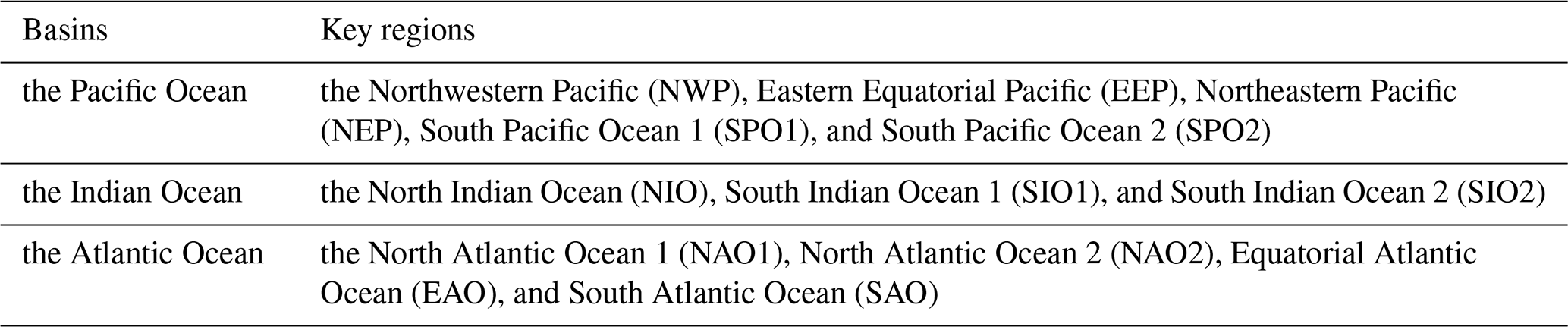
Based on the spatial patterns of oceanic CO₂ outgassing, uptake, and low-flux regimes characterized in the Pacific (Fig. 2c), this study delineates 12 key regions exhibiting high air–sea CO₂ flux variability as identified by NOAA CT2022 (Fig. 2d). These are selected from the 30 ocean basins defined in the CT2022 model documentation (Jacobson et al., 2023) for optimizing flux inversions. These oceanic domains are categorized into three major basins: (1) the Pacific Ocean, (2) the Indian Ocean, and (3) the Atlantic Ocean (Table 1). Within the Pacific basin, specific labels denote regions exhibiting the most pronounced oceanic CO₂ outgassing (the Equatorial Eastern Pacific, EEP) and uptake (the Northeastern Pacific, NEP).

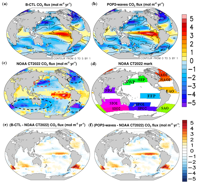
Figure 2 Climatological mean air–sea CO₂ flux (mol m⁻² yr⁻¹; shaded) and monthly standard deviation (SD; contour): (a) B–CTL; (b) POP2–waves; (c) NOAA CT2022: red dashed lines highlight the primary oceanic CO₂ outgassing and uptake regions in the Pacific Ocean, while black dashed lines mark regions with an air–sea CO₂ flux below −2 mol m⁻² yr⁻¹; (d) based on NOAA CT2022, 12 key regions exhibiting significant air–sea CO₂ flux variability have been identified among the 30 ocean basins defined in the CT2022 model documentation (Jacobson et al., 2023) for optimizing flux inversions. These include: (1) Pacific Ocean: Northwestern Pacific (NWP), Eastern Equatorial Pacific (EEP), as well as Northeastern Pacific (NEP), South Pacific Ocean 1 (SPO1), and South Pacific Ocean 2 (SPO2); (2) Indian Ocean: North Indian Ocean (NIO), South Indian Ocean 1 (SIO1), and South Indian Ocean 2 (SIO2); (3) Atlantic Ocean: North Atlantic Ocean 1 (NAO1), North Atlantic Ocean 2 (NAO2), Equatorial Atlantic Ocean (EAO), and South Atlantic Ocean (SAO), (e) the air–sea CO₂ flux difference between B–CTL and NOAA CT2022, and (f) same as (e), but between POP2–waves and NOAA CT2022.

Table 1 Characteristics of the 12 key regions exhibiting prominent air–sea CO₂ flux variability across the three major ocean basins.

3 Results

3.1 The climatological mean and seasonal variations of air–sea CO₂ flux

We utilize the traditional air–sea CO₂ flux bulk formula (Eq. 1) in CESM1.2.2 while also incorporating wave- and bubble-mediated effects via a gas transfer velocity parameterized by u^*, SST, and H_s (Eq. 3). A comparison of the climatological means and monthly standard deviations indicates that the spatial distribution of the model-simulated air–sea CO₂ fluxes is broadly consistent with NOAA CT2022, with regional differences generally remaining below 0.5 mol m⁻² yr⁻¹ across most analyzed sub-basins (Fig. 2a–f). Notably, the Pacific CO₂ outgassing and uptake regions simulated by the POP2–waves experiment show smaller range-normalized relative biases (Table 3) against NOAA CT2022 than the B–CTL baseline across most selected regions. This improvement occurs despite POP2–waves having a higher monthly SD across both the Pacific and Indian Oceans.

To ensure an objective and reproducible classification, the 12 ocean regions were categorized into two distinct groups based on rigid statistical criteria, requiring either seasonal phasing consistency or model–data absolute bias magnitudes relative to the NOAA CT2022 baseline to be met:

1. Seasonal phasing consistency (temporal alignment): Regulated by the Pearson correlation coefficient (r) between the simulated monthly flux cycles and NOAA CT2022. Regions assigned to Fig. 3 exhibit consistent seasonal phasing with significantly positive correlations (r≥0.50), whereas regions in Fig. 4 display prominent phase mismatches or anti-correlated trends (r<0.50 or statistically non-significant r).

2. Relative magnitudes of model–data biases (amplitude deviancy): Defined as the monthly averaged absolute deviation normalized by the overall peak-to-peak seasonal range (95th minus 5th percentile) of the NOAA CT2022 baseline. A threshold of 25 % was applied to further distinguish regions where structural amplitude offsets dominate over temporal phase alignment.

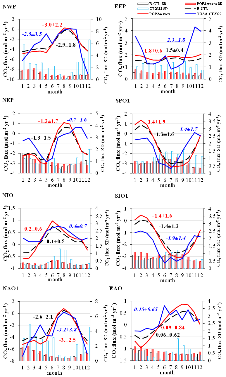
Figure 3 Climatological monthly mean CO₂ flux for eight highly correlated regions defined in Fig. 2d (NWP, EEP, NEP, SPO1, NIO, SIO1, NAO1, and EAO). Lines indicate values for B–CTL (black dashed), POP2–waves (red solid), and NOAA CT2022 (blue solid). Regional-average values are distinguished by a black font for B–CTL, red font for POP2–waves, and blue italics for NOAA CT2022. Monthly standard deviation (SD) is shown as bars: black hollow (B–CTL), red solid (POP2–waves), and light blue hollow (NOAA CT2022).

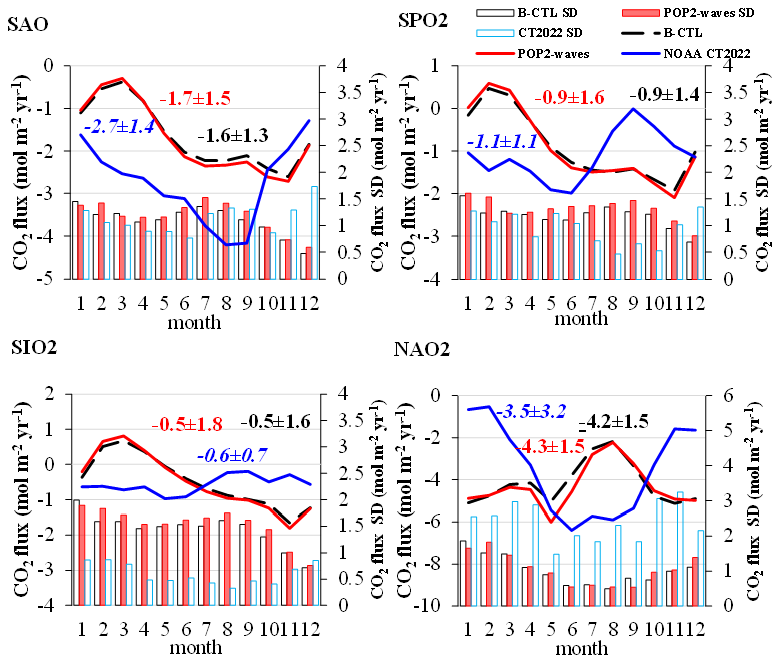
Figure 4 Same as Fig. 3, but for the four low-correlation characteristic regions (SAO, SPO2, SIO2, and NAO2), showing the climatological average of the simulated CO₂ flux compared with NOAA CT2022. Note: SAO, South Atlantic Ocean; SPO2, South Pacific Ocean Region 2; SIO2, South Indian Ocean Region 2; NAO2, North Atlantic Ocean Region 2.

Based on these thresholds, the eight regions in Fig. 3 exhibit coherent seasonal phasing and relatively small monthly model–data biases. In contrast, the four regions in Fig. 4 (including the South Atlantic Ocean with r=0.33) display clear structural discrepancies, such as inverted seasonal trends or weak temporal alignment. Importantly, these temporal phase misalignments tend to amplify the calculated monthly model–data biases, as the model and data fluctuate in opposing directions throughout the annual cycle. This phase mismatch contributes to larger relative monthly mean biases; specifically, the model–data biases averaged across the four regions in Fig. 4 (33.7 % in B–CTL and 32.6 % in POP2–waves) are markedly larger than those in the eight regions of Fig. 3 (26.4 % in B–CTL and 22.0 % in POP2–waves).

In terms of the regional mean values of air–sea CO₂ flux, the POP2–waves simulation generally demonstrates closer structural agreement with NOAA CT2022 compared to the uncoupled B–CTL baseline, showing improvements in seven of the eight analyzed regions (with the exception of the Northwest Pacific (NWP); Fig. 3). Nevertheless, despite this larger mean offset in specific regions such as the NWP, POP2–waves successfully captures the autumn transition of oceanic CO₂ from a sink to a source as depicted in NOAA CT2022 – a feature that remains unrepresented in B–CTL. Table 3 presents the range-normalized relative magnitudes of model–data biases across eight selected regions, providing a robust metric to evaluate the simulated seawater carbonate system, pH and flux field performance against the NOAA CT2022 atmospheric inversion baseline. Overall, the wave-coupled framework (POP2–waves) demonstrates a widespread reduction in systematic biases across the majority of the analyzed regions compared to the uncoupled control simulation (B–CTL). Specifically, the regional mean absolute deviation dropped noticeably in major ocean basins, with the most pronounced improvement captured in the Equatorial Eastern Pacific (EEP), where the relative bias was drastically attenuated by 25.0 % (from 71.5 % in B–CTL down to 46.5 % in POP2–waves). Notable bias reductions are also observed in the Northwest Pacific (NWP, down by 4.9 %), and South Indian Ocean Region 1 (SIO1, down by 4.1 %), confirming that incorporating wave-effect mechanisms successfully rectifies over- or under-estimations in air–sea carbon exchange dynamics. Conversely, the uncoupled baseline (B–CTL) exhibits slightly smaller biases in the Equatorial Atlantic Ocean (EAO) (11.9 % vs. 15.0 %), suggesting potential localized over-compensations in wave parameterizations within this sub-basin. Nonetheless, the reduction of relative biases across most other regions indicates that the online-coupled framework generally provides an improved representation of air–sea CO₂ fluxes.

The POP2–waves simulation generally exhibits a higher SD than B–CTL, reflecting an amplified seasonal variability (Figs. 3–4). Although these SD values typically remain below 3 mol m⁻² yr⁻¹, they peak during boreal winter, driven by intense oceanic CO₂ uptake in high-latitude regions of the Northern Hemisphere, such as the Northwestern and Northeastern Pacific, and the North Atlantic Ocean 1. In contrast, the Southern Hemisphere exhibits pronounced monthly SD along with clear oceanic CO₂ uptake during the austral winter (boreal summer), particularly across regions such as the South Pacific Ocean 1 (SPO1), South Indian Ocean 1 (SIO1), and South Atlantic Ocean (SAO). However, the monthly SD derived from NOAA CT2022 shows notable regional variations. In particular, both models underpredict the magnitude of variability observed in the Northwest Pacific (NWP), Equatorial Eastern Pacific (EEP), and North Atlantic Ocean 1 (NAO1).

Four specific sub-basins – South Atlantic Ocean (SAO), South Pacific Ocean Region 2 (SPO2), South Indian Ocean Region 2 (SIO2), and North Atlantic Ocean Region 2 (NAO2) – exhibit prominent model–data discrepancies when evaluated against NOAA CT2022 (Fig. 4). Notably, these systematic deviations are not attributable to wave-mediated processes or the parameterization of the CO₂ flux bulk formula. Within the NAO2, both the B–CTL and POP2–waves models simulate strong seasonal variations that mirror NAO1, characterized by substantial oceanic CO₂ uptake during the boreal winter; conversely, NOAA CT2022 displays the opposite seasonal trajectory in this sub-basin. A structurally similar mismatch is observed in the mid-latitude South Pacific (SPO2 and SIO2), where the simulated seasonal cycles of both models exhibit close synchronization with their respective low-latitude counterparts (SPO1 and SIO1) but differ noticeably from the inverse trend captured by the NOAA CT2022 atmospheric inversion framework.

3.2 The relationship between U₁₀ and k_w,660 in two regions with contrasting wind speed regimes

To demonstrate that the sea-state-dependent gas transfer velocity (Deike and Melville, 2018) provides a more suitable estimate of air–sea CO₂ flux than the wind-only formulation (Wanninkhof, 1992) under high-wind conditions (U₁₀>10 m s⁻¹), we selected the Western Pacific (WP) and the Equatorial Pacific (EP) regions due to their contrasting wind regimes. The WP region experiences a high frequency of high-wind conditions (exceeding 30 %), whereas wind speeds in the EP region consistently remain below this threshold. Because both regions exhibit stable and significant oceanic CO₂ outgassing or uptake, they enable a clear comparative analysis of the correlation between k_w,660 and U₁₀ (Fig. 5a, b).

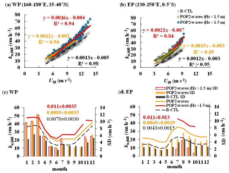
Figure 5 Scatter plots of monthly averaged gas transfer velocity (k_w,660) versus U₁₀ for (a) the Western Pacific (WP; 160–180° E, 35–40° N) and (b) the Eastern Pacific (EP; 230–250° E, 0–5° S). Gray open circles, green open squares, and blue dots with black edges represent B–CTL, POP2–waves data for H_s<1.5 m, and H_s>1.5 m, respectively. Corresponding simple linear regressions (SLRs) and squared correlation coefficients (R²) are shown with black dotted lines/text (B–CTL), orange solid lines/text (POP2–waves, H_s<1.5 m), and red solid lines/text (POP2–waves, H_s>1.5 m). Panels (c) and (d) display the monthly mean values of k_w,600 for WP and EP, respectively. Red and orange solid lines/text indicate POP2–waves (H_s>1.5 m) and the average of all POP2–waves data, while the black dotted line/text represents B–CTL. The bar graph illustrates the standard deviation (SD) for each month over the WP and EP, red hollow bars for POP2–waves (H_s>1.5 m), orange for average POP2–waves, and black for B–CTL.

Generally, the B–CTL data shows higher R² but lower k_w,660 values compared to those in POP2–waves across both the WP and EP. The POP2–waves experiment exhibits a slightly lower R² than B–CTL due to greater deviations between k_w,660 and U₁₀, particularly at higher surface wind speeds. This pattern is consistent with the findings of Gutiérrez-Loza et al. (2022) under conditions where H_s>1.5 m. The relationship between k_w,660 and U₁₀ was evaluated under two scenarios: baseline monthly climatological means (H_s<1.5 m) and high-resolution daily data filtered for H_s>1.5 m (enhanced conditions) aggregated into 30-year monthly averages. Notably, both approaches substantially diminish the differences in k_w,660 at identical U₁₀ values.

However, short-term (30 min) observations indicate that gas transfer velocity can be up to twice as high under similar wind speeds when H_s>1.5 m (Gutiérrez-Loza et al., 2022). Divergence between the models becomes significant when U₁₀ exceeds 12 m s⁻¹ over the WP region (Fig. 5a), whereas over the EP region, the convergence of k_w,660 estimates is most notable around U₁₀=9 m s⁻¹ (Fig. 5b), suggesting that mid-range wind speeds dominate the EP flux signal.

As shown in Fig. 5c, the enhanced WP cases (H_s>1.5 m) have data available for all months except August and October, during these available months, their k_w,660 values consistently exceed both the all-data POP2–waves and B–CTL averages. In contrast, the EP region exhibits H_s>1.5 m data only during the summer months (July to October), where corresponding k_w,660 values also exceed both all-data POP2–waves and B–CTL averages. The monthly SD indicates no significant differences between the enhanced (H_s>1.5 m) data and the standard POP2–waves simulations over the WP, with the k_w,660 discrepancies between the two datasets remaining minimal from January to May because the average H_s during this period consistently remains below 1.5 m. However, over the EP, a pronounced discrepancy is observed between the H_s>1.5 m condition and the all-data POP2–waves average from July to September.

3.3 Regression of CO₂ flux against U₁₀ under high-wind conditions

The wind-only parameterization of gas transfer velocity tends to underestimate values under high-wind conditions (U₁₀>10 m s⁻¹) or high significant wave heights (H_s>1.5 m) (e.g., Gutiérrez-Loza et al., 2022; Zhou et al., 2023). Under these high-wind conditions, the monthly mean air–sea CO₂ fluxes derived from the B–CTL and POP2–waves simulations diverge notably within the Western Pacific region (WP) (Fig. 6), highlighting key discrepancies between the wind-only and wave-modified k_w,660 formulations. The data were filtered to include only grid points that met this high-wind threshold before being regionally averaged. Because not all months contained grid points satisfying the threshold, a final subset of 154 data points was utilized for the linear regression analysis. These high-wind conditions over the WP region occur primarily in winter (accounting for 42 % of the valid data), when the concurrent low sea surface temperatures further enhance CO₂ solubility. The slopes of the regression equations (−0.77 mol m⁻³ s yr⁻¹ for B–CTL and −1.40 mol m⁻³ s yr⁻¹ for POP2–waves) alongside the mean CO₂ fluxes (Y_avg: −6.35 mol m⁻² yr⁻¹ for B–CTL and −6.97 mol m⁻² yr⁻¹ for POP2–waves) both indicate that POP2–waves exhibits a higher sensitivity to wind speed, leading to stronger oceanic CO₂ uptake across the WP domain under elevated wind speeds.

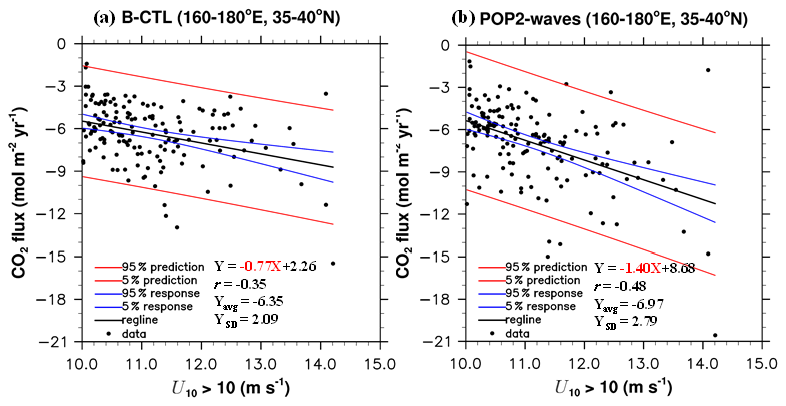
Figure 6 Scatter plots of air–sea CO₂ flux versus U₁₀ with regression lines over the Western Pacific (160–180° E, 35–40° N) under high-wind conditions (U₁₀>10 m s⁻¹) for (a) B–CTL and (b) POP2–waves experiments. Black dots indicate monthly mean values from each experiment. Blue lines denote the 95 % and 5 % confidence limits of the mean response, while red lines denote the 95 % and 5 % prediction intervals. The regression equation ($Y=mx+b$), Pearson correlation coefficient (r), mean CO₂ flux (Y_avg), and standard deviation (Y_SD) are shown to the right of the legend.

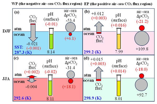
The correlation coefficient (R) of the POP2–waves simulation is higher than that of B–CTL, indicating that the sea-state-dependent k_w,660 formulation provides a more realistic representation of the CO₂ flux than the wind-only k_w,660 scheme under high-wind conditions. This finding aligns with the observations of Gutiérrez-Loza et al. (2022) and Zhou et al. (2023). The average air–sea CO₂ flux in B–CTL over the WP region during DJF and JJA is −0.021 and −0.004 mol m⁻² yr⁻¹, respectively. Meanwhile, POP2–waves exhibits only slight discrepancies relative to B–CTL during these respective seasons, with differences ranging between 0.001 and 0.002 mol m⁻² yr⁻¹ in CO₂ uptake (data not shown). This contrast indicates that under high-wind conditions, the episodic air–sea CO₂ flux is significantly greater than the seasonal baseline averages.

3.4 Analysis of surface fields and k_w,660 component in POP2–waves and B–CTL

The spatial co-variations of sea level pressure (SLP), U₁₀, and H_s underscore their combined role as key meteorological and wave drivers steering the regional k_w,660 patterns (Fig. 7a, b). The region with H_s>1.5 m is generally situated where U₁₀>8 m s⁻¹ and lies south of the high-SLP region. The spatial patterns of climatological U₁₀ and H_s align closely with the findings of Reichl and Deike (2020) (Fig. 7a, b). Furthermore, a dominance of bubble-mediated transfer in the POP2–waves simulation, where the $k_{\mathrm{wB},\mathrm{660}}/k_{\mathrm{w},\mathrm{660}}$ ratio exceeds 0.5, primarily occurs in regions characterized by H_s>1.5 m (Fig. 7b). However, an elevated H_s does not always correspond to a higher $k_{\mathrm{wB},\mathrm{660}}/k_{\mathrm{w},\mathrm{660}}$ ratio in the POP2–waves simulation; this decoupling is explicitly observed in the North Pacific (Fig. 7b).

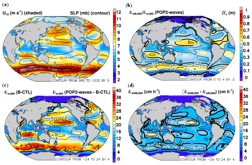
Figure 7 Effects of atmospheric factors and wave components on average gas transfer velocity: (a) Shaded areas represent 10 m wind speed (U₁₀, m s⁻¹) and contours show sea level pressure (SLP, mb); (b) color denotes the ratio of bubble-mediated (k_wB,660) to POP2–waves k_w,660 components, with contours representing significant wave height H_s (m) and thick lines marking H_s=1.5 m; (c) shading represents k_w,660 (B–CTL) and contours represent the difference k_w,660 (POP2–waves − B–CTL) in cm hr⁻¹; (d) shading shows the non-bubble-mediated component (k_wNB,660) and contours show the difference ($k_{\mathrm{wNB},\mathrm{660}}-k_{\mathrm{wB},\mathrm{660}}$) in cm hr⁻¹, with the thick contour lines at 0.

Deike and Melville (2018) demonstrated that the bubble contribution to CO₂ transfer exceeds 40 % when the U₁₀≥10 m s⁻¹. In our POP2–waves simulation, the bubble fraction ($k_{\mathrm{wB},\mathrm{660}}/k_{\mathrm{w},\mathrm{660}}$) accounts for approximately 38 % of total gas transfer velocity, which is slightly higher than the ∼30 % reported by Reichl and Deike (2020). This discrepancy may be attributed to differences in the A_B scaling coefficients (Eq. 3), which are derived from field data, where gas transfer velocity is estimated from eddy covariance flux measurements (Reichl and Deike, 2020; Brumer et al., 2017).

The structural differences in k_w,660 (POP2–waves − B–CTL) reveal that the most pronounced discrepancies are primarily distributed in regions characterized by elevated H_s, particularly in the Southern and South Indian Oceans (Fig. 7c). Although U₁₀ in the Indian Ocean and tropical Pacific is relatively low (<5 m s⁻¹; Fig. 7a), the k_w,660 values simulated by POP2–waves remain approximately 9 cm hr⁻¹ higher than those in B–CTL. In these regions, this wave-driven enhancement of the total gas transfer velocity is predominantly governed by the non-bubble-mediated component (k_wNB,660; Fig. 7d). Although H_s is also elevated in the Southern Ocean (Fig. 7b), it does not contribute substantially to the k_w,660 difference between POP2–waves and B–CTL; this is because the high U₁₀ in this region (Fig. 7a) already yields high gas transfer velocities through the empirical formulation of Wanninkhof (1992). The spatial patterns of both the B–CTL k_w,660 and the wave-induced k_w,660 discrepancies (POP2–waves − B–CTL) closely align with the findings of Reichl and Deike (2020) (Fig. 7c). Overall, the two simulations exhibit consistent geographic distributions, yielding 30-year domain-wide mean gas transfer velocities of 17.0 cm hr⁻¹ for B–CTL and 22.7 cm hr⁻¹ for POP2–waves, despite their reliance on distinct input parameters (U₁₀ versus u^* and H_s). Aside from the polar regions, the total gas transfer velocity in the POP2–waves coupled model exceeds that in B–CTL, with the most pronounced differences localized in the tropics (Fig. 7c). To elucidate the driving mechanisms behind this global enhancement, it is necessary to quantify whether the non-bubble (k_wNB,660) or bubble-mediated (k_wB,660) component dominates the total gas transfer velocity across the different ocean basins. This partitioning demonstrates that bubble-mediated processes dominate ($k_{\mathrm{wB},\mathrm{660}}>k_{\mathrm{wNB},\mathrm{660}}$) under high-H_s conditions, whereas non-bubble mechanisms prevail ($k_{\mathrm{wB},\mathrm{660}}<k_{\mathrm{wNB},\mathrm{660}}$) in light-wind zones where U₁₀<7 m s⁻¹ (Fig. 7).

3.5 Mean State and model differences in $p{\mathrm{CO}}_{\mathrm{2}}^{\mathrm{w}}$ and surface pH

Integrating wave dynamics induces a pronounced spatial reorganization of both $p{\mathrm{CO}}_{\mathrm{2}}^{\mathrm{w}}$ and ocean surface pH over the 30-year climatological period (Fig. 8). Specifically, the baseline B–CTL simulation shows that high $p{\mathrm{CO}}_{\mathrm{2}}^{\mathrm{w}}$ is concentrated in the equatorial eastern Pacific (EEP), contributing to a larger oceanic CO₂ source (Fig. 8a). In contrast, low $p{\mathrm{CO}}_{\mathrm{2}}^{\mathrm{w}}$ is found in high-latitude regions of the Pacific and Atlantic (e.g., NWP, NEP, NAO1, and NAO2), driving strong oceanic CO₂ uptake (Fig. 8a). Over the study period, the climatological standard deviation of $p{\mathrm{CO}}_{\mathrm{2}}^{\mathrm{w}}$ in B–CTL ranges between 10 and 30 ppm (Fig. 8a).

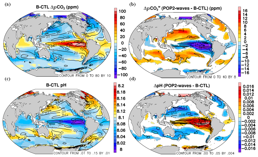
Figure 8 Spatial distributions of the 30-year climatological averages and model differences for $\mathrm{\Delta }p{\mathrm{CO}}_{\mathrm{2}}^{\mathrm{w}}$ (ppm; panels a, b) and ocean surface pH (panels c, d). Climatological means are represented by shading, and their corresponding standard deviation (SD) is superimposed as contours. Panels (a) and (c) present baseline results from the B–CTL simulation. Panels (b) and (d) depict the structural differences between the POP2–waves and B–CTL experiments (POP2–waves minus B–CTL), where stippling indicates statistical significance at the 95 % confidence level based on a Student's t-test.

In the CESM1 framework of the B_2000_CAM5 compsets, atmospheric $p{\mathrm{CO}}_{\mathrm{2}}^{\mathrm{a}}$ is held constant (367 ppm). The $p{\mathrm{CO}}_{\mathrm{2}}^{\mathrm{w}}$ in the Eastern Pacific exceeds 440 ppm, indicating an air–sea ΔpCO₂ greater than 73 ppm in B–CTL (109.8 and 92.7 ppm during DJF and JJA, respectively), whereas the $p{\mathrm{CO}}_{\mathrm{2}}^{\mathrm{w}}$ in the Western Pacific is below 320 ppm, indicating an air–sea ΔpCO₂ lower than −47 ppm (−53.4 and −31.4 ppm during DJF and JJA, respectively). Notably, POP2–waves reduces the high $p{\mathrm{CO}}_{\mathrm{2}}^{\mathrm{w}}$ by more than 10 ppm over the Eastern Equatorial Pacific and increases the low $p{\mathrm{CO}}_{\mathrm{2}}^{\mathrm{w}}$ in other regions (Fig. 8b). Consequently, in the oceanic CO₂ outgassing (uptake) regions, the POP2–waves coupled model decreases (increases) $p{\mathrm{CO}}_{\mathrm{2}}^{\mathrm{w}}$, thereby reducing the magnitude of the air–sea ΔpCO₂. The climatological SD of the $p{\mathrm{CO}}_{\mathrm{2}}^{\mathrm{w}}$ discrepancy between POP2–waves and B–CTL displays marked spatial variability over the Eastern Equatorial Pacific, whereas changes across other regions remain relatively minor.

The biogeochemical module of POP2 (BEC) updates TA in each grid cell by solving a coupled transport–reaction equation (Moore et al., 2013). The average pH of the ocean is currently around 8.1 in oceanic CO₂ uptake regions (e.g., the Western Pacific) and 8.0 in outgassing regions (e.g., the Equatorial Pacific; Fig. 8c), reflecting slightly alkaline conditions. Within the DIC system, bicarbonate ions (HCO${}_{\mathrm{3}}^{-}$) are the dominant species because background seawater pH falls strictly between pK_a1 and pK_a2. However, continued uptake of atmospheric CO₂ drives a decline in pH – a process termed ocean acidification. Our study highlights that wave-induced k_w,660 significantly influences the marine CO₂ system, altering alkalinity, pH, and carbonate speciation. These chemical shifts, in turn, provide a feedback mechanism that modulates the overall dynamics of the air–sea CO₂ flux. Consequently, wave-driven perturbations in k_w,660 directly alter both ΔpCO₂ and net air–sea CO₂ fluxes within the Earth System Model framework.

Ocean pH and surface ocean $p{\mathrm{CO}}_{\mathrm{2}}^{\mathrm{w}}$ are strongly negatively correlated (Macovei et al., 2021). Consequently, low pH values are observed in the Equatorial Eastern Pacific (Fig. 8c), as a direct result of the elevated DIC and $p{\mathrm{CO}}_{\mathrm{2}}^{\mathrm{w}}$ concentrations characteristic of that region (Fig. 8a). Conversely, elevated pH conditions persist in domains with lower $p{\mathrm{CO}}_{\mathrm{2}}^{\mathrm{w}}$, a signature most prominent throughout high-latitude waters in both the Pacific and Atlantic Basins. Rustogi et al. (2025) indicate that accelerated equilibration of oceanic pCO₂ in the wind–wave–bubble simulation, driven by enhanced gas exchange, ultimately reduces the magnitude of the air–sea ΔpCO₂. This pCO₂ feedback is strongest in the extratropics, where it suppresses CO₂ uptake. Our POP2–waves experiment reveals a consistent response, characterized by increases in both oceanic pCO₂ (Fig. 8b) and hydrogen ion concentration ([H⁺]), which are accompanied by a corresponding decline in pH (Fig. 8d) throughout the extratropical ocean basins. Accounting for wave effects results in simulated pH shifts of approximately +0.01 (−0.01) in oceanic CO₂ outgassing (uptake) regions (Fig. 8d). This suggests that incorporating this mechanism alleviates acidification in the equatorial Pacific, whereas it intensifies ocean acidification in the high-latitude domains of both the Pacific and Atlantic Oceans (Fig. 8d). Rustogi et al. (2025) also showed that the effects of Δk_w (the difference between wave-induced k_w,660 and k_w,660 based on U₁₀) and ΔpCO₂ (POP2–waves − B–CTL) partially offset each other. However, because the Δk_w effect is generally 20 %–30 % stronger, it dominates the counteracting ΔpCO₂ effect, explaining the modest changes observed in both oceanic outgassing and uptake CO₂ fluxes within the wave-effect simulation.

4 Discussion

4.1 Impact of wave-dependent k_w on global air–sea CO₂ flux: a comparison between POP2–waves and standard Earth System Models

Several investigations have parameterized the air–sea CO₂ flux using Eq. (1), yet current k_w,660 parameterizations within prominent global frameworks still rely exclusively on the neutral 10 m wind speed (U₁₀) as seen in models such as MPI-ESM1.2 (Mauritsen et al., 2019), CESM2 (Danabasoglu et al., 2020), NorESM2 (Seland et al., 2020), UKESM1 (Sellar et al., 2019), MIROC6 (Chikamoto and DiNezio, 2021), CMCC-ESM2 (Lovato et al., 2022), and CanESM5 (Sigmond et al., 2023) (Table 2). Concurrently, pioneering efforts have begun quantifying wave-induced effects on both air–sea CO₂ flux and long-term ocean carbon storage by incorporating coupled wind–wave–bubble gas transfer formulations into ocean general circulation models (OGCMs), such as MOM6–COBALTv2 (Rustogi et al., 2025) and NEMO–PISCES (Wu et al., 2025). Importantly, Wu et al. (2025) emphasize that integrating these wave-mediated boundary layer dynamics into fully coupled Earth System Models is crucial to reducing systemic uncertainties in global carbon cycle projections.

Table 2 Intercomparison of Earth System Model for estimating air–sea CO₂ flux

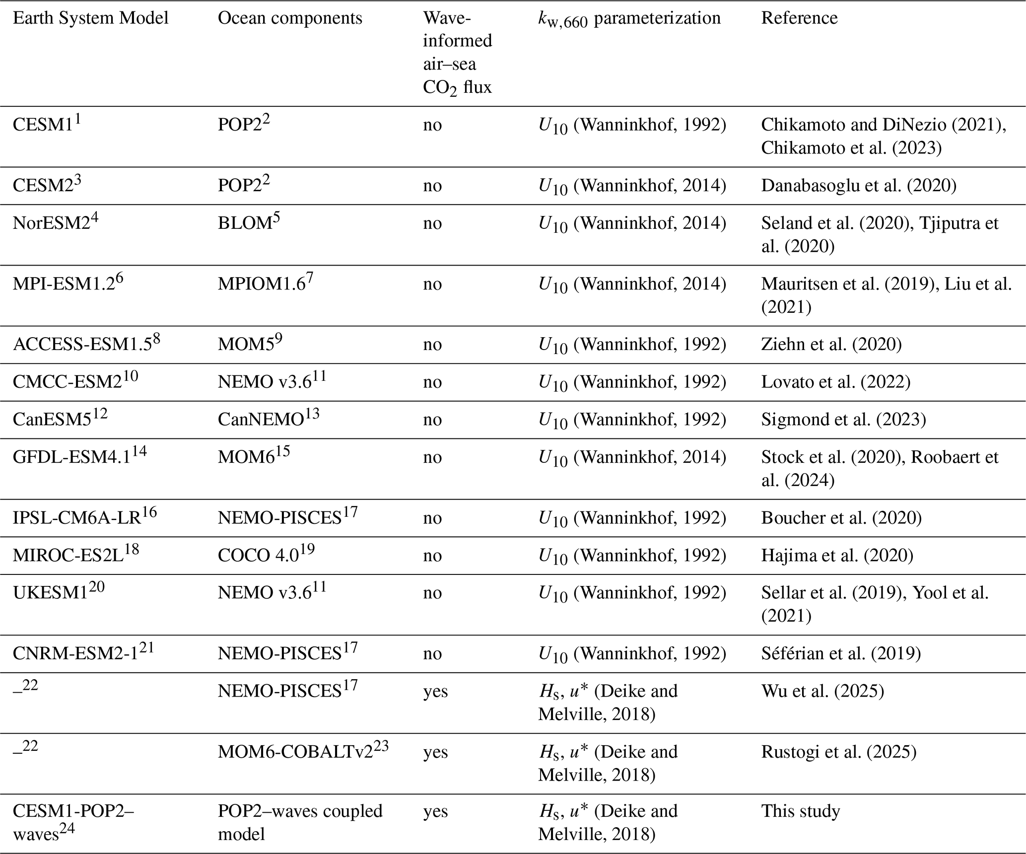
Note: ¹ CESM1: the Community Earth System Model version 1 of the National Center for Atmospheric Research (NCAR); ² POP2: the Parallel Ocean Program version 2 of NCAR; ³ CESM2: CESM version 2; ⁴ NorESM2: The Norwegian Earth System Model version 2; ⁵ BLOM: Bergen Layered Ocean Model; ⁶ MPI-ESM1.2: the Max Planck Institute for Meteorology Earth System Model version 1.2; ⁷ MPIOM1.6: the Max-Planck Institute Ocean Model version 1.6; ⁸ ACCESS-ESM1.5: the Australian Community Climate and Earth System Simulator form an Earth System Model version 1.5; ⁹ MOM5: the GFDL Modular Ocean Model version 5; ¹⁰ CMCC-ESM2: the Euro-Mediterranean Centre on Climate Change (CMCC) Earth System Model version 2; ¹¹ NEMO v3.6: Nucleus for European Modelling of the Ocean version 3.6; ¹² CanESM5: the Canadian Earth System Model version 5; ¹³ CanNEMO: NEMO version 3.4 modified for CanESM; ¹⁴ GFDL‐ESM4.1: the Geophysical Fluid Dynamics Laboratory's Earth System Model 4.1; ¹⁵ MOM6: the GFDL Modular Ocean Model version 6; ¹⁶ IPSL‐CM6A‐LR : version 6 of the Institut Pierre-Simon Laplace (IPSL) climate model; ¹⁷ NEMO-PISCES: Nucleus for European Modelling of the Ocean, Pelagic Interaction Scheme for Carbon and Ecosystem Studies ocean general circulation and biogeochemistry model; ¹⁸ MIROC-ES2L: the Model for Interdisciplinary Research on Climate, Earth System version 2; ¹⁹ COCO 4.0: CCSR (Center for Climate System Research) Ocean Component Model version 4.0; ²⁰ UKESM1: the U.K. Earth System Model; ²¹ CNRM-ESM2-1: the Earth system (ES) model of second generation developed by the Centre National de Recherches Météorologiques (CNRM); ²² The simulations were conducted using global ocean-only models rather than full Earth System Models; ²³ MOM6-COBALTv2: Geophysical Fluid Dynamics Laboratory global ocean model (Modular Ocean Model, MOM6) coupled with sea ice and biogeochemistry (Carbon, Ocean Biogeochemistry and Lower Trophics version 2, COBALTv2); ²⁴ CESM1-POP2–waves: POP2–waves coupled model based on CESM1.

Table 3 Relative magnitudes of model–data biases (%), defined as the monthly mean absolute deviation normalized by the model's corresponding monthly variability range (95th minus 5th percentile).

Note: Abbreviations: NWP: Northwestern Pacific; EEP: Eastern Equatorial Pacific; NEP: Northeastern Pacific; SPO1: South Pacific Ocean 1; NIO: North Indian Ocean; SIO1: South Indian Ocean 1; NAO1: North Atlantic Ocean 1; EAO: Equatorial Atlantic Ocean. The relative magnitude of model–data bias (%) across the 360-month period is defined and calculated as follows:

$$\begin{array}{}\text{(7)}& \text{Model-data biases}\left(\mathit{\%}\right)={\displaystyle \frac{\mathrm{1}}{\mathrm{12}}}\sum _{i=\mathrm{1}}^{\mathrm{12}}{\displaystyle \frac{|M_i-O_i|}{P_{\mathrm{95}}\left(M\right)-P_{\mathrm{5}}\left(M\right)}}\end{array}$$

where M_i and O_i represent the monthly mean values simulated by (POP2–waves or B–CTL) and reference (the NOAA CT2022 inversion) air–sea CO₂ fluxes for the month mean of month i ($i=\mathrm{1},\mathrm{2},\mathrm{\dots },\mathrm{12}$), respectively. P₉₅ (M) and P₅(M) denote the 95th and 5th percentiles, respectively, of each calendar month's values over the 30-year period, representing the corresponding range of monthly variability in the model.

Several studies have incorporated wave effects following the parameterization of Deike and Melville (2018), utilizing the Surface Ocean CO₂ Atlas (SOCAT) database (Bakker et al., 2016) to calculate diagnostic air–sea CO₂ fluxes. In these offline configurations, however, the computed air–sea CO₂ flux is treated independently of $p{\mathrm{CO}}_{\mathrm{2}}^{\mathrm{w}}$ dynamics and surface pH evolution, lacking any interactive feedback mechanisms between the atmosphere and the upper-ocean carbonate system.

Rustogi et al. (2025) utilized an ocean-biogeochemistry system forced by offline atmospheric reanalysis and wave model outputs. While comprehensive, such an offline-forced setup is limited in its ability to capture high-frequency, episodic, and synchronous interactions between physical wave states and surface water chemistry during rapid weather transitions. In contrast, our study implements an online coupling framework. The key added value of our setup is its capacity to simulate step-by-step interactive feedbacks where wave properties dynamically alter the gas transfer velocity (k_w,660) and physical mixing in real-time. The coupled behavior of POP2–waves includes ΔpCO₂-driven negative feedbacks, which fundamentally differs from traditional obs-based products that treat wave-induced k_w,660 and ΔpCO₂ as independent variables when estimating air–sea CO₂ flux (e.g., Reichl and Deike, 2020). This online coupling mechanism also contrasts with global ocean models forced offline by atmospheric reanalysis and wave model outputs (e.g., Rustogi et al., 2025), where such interactive feedbacks are often omitted. This approach enables our model to resolve non-linear, high-resolution modulations of air–sea CO₂ exchange during rapid dynamic events – effects that are typically muted in offline configurations.

4.2 Impact of air–sea ΔpCO₂, k_w,660, SST, and pH on air–sea CO₂ flux

To evaluate which driver exerts the most direct control on air–sea CO₂ flux, Fig. 9 displays the spatial distributions of the linear regression coefficients (LRCs) derived from univariate (one-on-one) linear regressions between the flux and various standardized variables: air–sea ΔpCO₂ (Fig. 9a), k_w,660 (Fig. 9b), SST (Fig. 9c), and pH (Fig. 9d). To remove the confounding artifacts of differing physical units and enable a direct comparison on a common scale, both the air–sea CO₂ flux and the independent variables were standardized into anomalies (with a mean of 0 and a standard deviation of 1) prior to the regression analysis. The statistical significance of these regressed relationships was subsequently evaluated using a Student's t-test at the 95 % confidence level. Because each standardized regression was performed individually with a single independent variable, the resulting LRCs are equivalent to Pearson correlation coefficients (r), constraining their values strictly between −1 and +1. Here, we do not delve into the intricate chemical and biochemical feedback mechanisms governing carbonate species. Nevertheless, it is worth noting that the collective influence of carbonate composition – specifically TA and dissolved inorganic carbon (DIC) – on $p{\mathrm{CO}}_{\mathrm{2}}^{\mathrm{w}}$ variability has been shown to outweigh that of solubility changes driven by sea surface salinity and SST (e.g., Koseki et al., 2023).

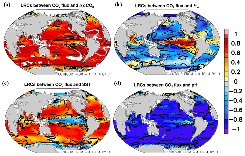
Figure 9 Spatial distributions of the 30-year averages of the linear regression coefficients (LRCs) between the CO₂ flux and (a) ΔpCO₂, (b) $k_{\mathrm{w},\mathrm{660}},$ (c) SST, and (d) pH. Shading represents the baseline LRCs from the B–CTL simulation, while overlaid contours depict the structural differences between the POP2–waves and B–CTL experiments (POP2–waves minus B–CTL). White areas denote regions where the LRCs are statistically insignificant at the 95 % confidence level (based on a Student's t-test). All variables were standardized prior to the regression analysis.

Among these drivers, air–sea ΔpCO₂ and air–sea CO₂ flux exhibit the strongest positive LRCs, with coefficients ranging from 0.6 to 0.8 across the global ocean; this underscores the ocean's role as a net CO₂ source or sink depending on the sign of the air–sea ΔpCO₂ gradient. Additionally, wave effects increase the LRCs by approximately 0.1 to 0.2, particularly within regions of intense oceanic CO₂ outgassing or uptake. Clear positive (negative) LRCs exist between k_w,660 and the air–sea CO₂ flux in oceanic CO₂ outgassing (uptake) regions. Furthermore, wave effects reduce the absolute LRCs between k_w,660 and air–sea CO₂ flux in both oceanic CO₂ outgassing (uptake) regions (Fig. 9b). This indicates that once interactions between the modeled CO₂ flux and the ocean carbonate–pH system are considered, the wave-influenced CO₂ flux becomes less correlated with k_w,660 and more closely linked to air–sea ΔpCO₂. This shift can be attributed to the limitations of wind-only parameterizations; as indicated by Zhou et al. (2023), wind-only formulas tend to underestimate gas transfer velocities when U₁₀ exceeds 10 m s⁻¹, where intense wave breaking and high significant wave height substantially boost air–sea gas exchange. Furthermore, Johansson et al. (2022) reported that H_s generally increases with wind speed, but the relationship is strongly modulated by wind direction and regional conditions, leading to spatially variable and nonlinear wind–wave coupling.

In contrast to the former, there are clear positive (negative) LRCs between SST and CO₂ flux in oceanic CO₂ uptake (outgassing) regions (Fig. 9c). A negative correlation exists between k_w,660 and SST, reflecting the latitudinal gradient where colder, high-latitude waters are characterized by more intense sea states and elevated k_w,660 values. This pattern occurs because lower temperatures at high latitudes increase CO₂ solubility, thereby enhancing oceanic uptake. From a thermodynamic perspective, higher SST enhances molecular diffusion while lowering seawater viscosity, thereby reducing the Schmidt number ($Sc=\mathit{\nu }/D$, defined as the ratio of kinematic viscosity (ν) to the molecular diffusion coefficient (D)). Because k_w,660 is parameterized as a function of Sc^−0.5, a decrease in Sc theoretically elevates k_w,660. Separately, Fay et al. (2024) attributed the regional discrepancies and variations in air–sea CO₂ fluxes to a combination of factors, including choices in wind speed products, SST datasets, biological carbon uptake, and the parameterization of gas transfer velocity. Wave effects only slightly reduce the LRCs between SST and the air–sea CO₂ flux – by approximately 0.1 – within the tropics, with negligible impacts observed in other regions. The strong negative correlation between ocean pH and $p{\mathrm{CO}}_{\mathrm{2}}^{\mathrm{w}}$ is dictated by the acid dissociation equilibria of the marine carbonate system (Fig. 8a, c), which govern the fundamental relationship between dissolved CO₂ and hydrogen ion concentration (Williams et al., 2017). As seawater pH decreases, the resulting increase in hydrogen ion concentration ([H⁺])reacts with carbonate ions (CO${}_{\mathrm{3}}^{\mathrm{2}-}$). This consumption of carbonate ions reduces the ocean's buffering capacity for CO₂ uptake, causing seawater $p{\mathrm{CO}}_{\mathrm{2}}^{\mathrm{w}}$ to increase. Because atmospheric $p{\mathrm{CO}}_{\mathrm{2}}^{\mathrm{a}}$ is fixed at 367 ppm in the CESM1.2.2 configuration, this rise in surface ocean $p{\mathrm{CO}}_{\mathrm{2}}^{\mathrm{w}}$ narrows the air–sea partial pressure gradient ΔpCO₂ in uptake regions (where seawater $p{\mathrm{CO}}_{\mathrm{2}}^{\mathrm{w}}$ is below atmospheric levels), thereby suppressing the air–sea CO₂ influx. Reflecting this mechanism, pH and air–sea CO₂ flux exhibit strong negative LRCs (less than −0.9) across most of the global ocean, with exceptions confined to the Eastern Equatorial Pacific and along the Arctic margins (Fig. 9d). Wave effects marginally attenuate this relationship in the Eastern Equatorial Pacific (EEP), reducing the LRCs by approximately 0.1.

4.3 Uncertainty arising from the absence of interactions between air–sea CO₂ flux and the ocean carbonate–pH system

Rustogi et al. (2025) indicate that as surface seawater $p{\mathrm{CO}}_{\mathrm{2}}^{\mathrm{w}}$ equilibrates with changes in DIC and alkalinity, the air–sea ΔpCO₂ gradient is partially attenuated. This induces a negative feedback loop whereby enhanced CO₂ uptake (or outgassing) is systematically damped by chemical re-equilibration within the marine carbonate system, a mechanism that is highly consistent with the findings of this study. To assess the uncertainty in CO₂ flux resulting from the absence of interactions between the flux and the ocean carbonate–pH system (i.e., the decoupling of the ΔpCO₂-driven negative feedback), we performed a series of sensitivity experiments. The air–sea CO₂ flux was reconstructed using the uncoupled ΔpCO₂ fields from the control simulation (B–CTL) and the wave-influenced k_w,660 parameterization from the coupled wave simulation (POP2–waves). This experimental setup explicitly isolates the statistical mean and standard deviation of the flux under a scenario defined by the “lack of ΔpCO₂-driven negative feedback”. Only data showing a statistically significant air–sea CO₂ flux difference (at a 95 % confidence level) between “lack of ΔpCO₂-driven negative feedback” scenario and POP2–waves are presented in Fig. 10b. Compared to the baseline (Fig. 2b), the CO₂ flux under the “lack of ΔpCO₂-driven negative feedback” scenario is stronger than that in the POP2–waves simulation across both oceanic CO₂ outgassing and uptake regions, accompanied by a larger SD. The most pronounced discrepancies occur in the Pacific basin across both outgassing and uptake zones. However, certain mid-to-high latitude subregions – specifically the Northeastern Pacific (NEP), South Indian Ocean 2 (SIO2), and South Pacific Ocean 2 (SPO2) – do not reach the 95 % confidence threshold.

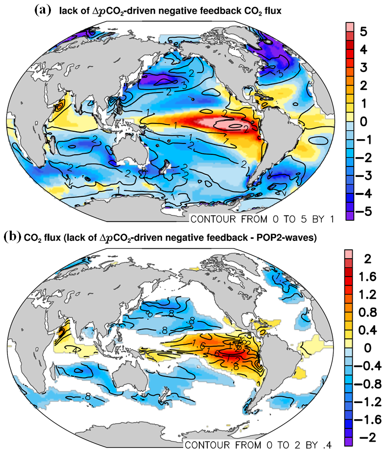
Figure 10 Estimated air–sea CO₂ flux assuming the absence of the ΔpCO₂-driven negative feedback mechanism. (a) Air–sea CO₂ flux calculated using uncoupled, independent ΔpCO₂ values from the B–CTL baseline and wave-dependent k_w,660 formulations (labeled as the “lack of ΔpCO₂-driven negative feedback” case). Shading represents the climatological mean, and contours indicate the corresponding standard deviation (SD). (b) Spatial difference in CO₂ flux between the decoupled feedback case and the fully coupled POP2–waves simulation (decoupled minus POP2–waves). Shading denotes the mean difference, and overlaid contours indicate regions where the difference is statistically significant at the 95 % confidence level based on a Student's t-test.

Rustogi et al. (2025) demonstrate that while wave-enhanced k_w,660 accelerates local air–sea CO₂ exchange, it simultaneously attenuates the air–sea ΔpCO₂ gradient. In this study, we conceptualize this process as a manifestation of the ocean's buffering capacity, which encompasses the dynamic coupling between CO₂ flux (estimated via k_w,660) and the marine carbonate–pH system. Within the coupled POP2–waves framework, incorporating wave effects alleviates surface acidification and reduces air–sea ΔpCO₂ over oceanic CO₂ outgassing regions; conversely, the resulting relatively higher pH levels systematically enhance the ocean's capacity to absorb atmospheric CO₂ within oceanic CO₂ uptake regions in the coupled POP2–waves model. In contrast, the simulation lacking the ΔpCO₂-driven negative feedback – which artificially omits realistic marine buffering effects – overestimates the air–sea exchange, yielding excess CO₂ outgassing into the atmosphere (>0.4 mol m⁻² yr⁻¹) over source regions. Concurrently, it amplifies excess CO₂ uptake ($<-\mathrm{0.4}$ mol m⁻² yr⁻¹) within regions characterized by oceanic CO₂ uptake regions (Fig. 10b) compared to the coupled POP2–waves model.

5 Conclusions

The study advances an Earth System Model (ESM) by developing an online coupling framework (POP2–waves) that incorporates wave effects directly into air–sea CO₂ flux simulations, capturing the ΔpCO₂-driven negative feedback within the marine carbonate–pH system. Diagnostically neglecting this coupling by treating ΔpCO₂ and wave-induced k_w,660 independently leads to a positive bias in global flux calculations, whereas our online coupled simulation captures a buffering negative feedback that moderates the global net response. Fully integrating these wave effects addresses three core modeling challenges:

1. Technical implementation: Resolving grid interpolation, boundary discontinuities in wave energy, and parallel computation.

2. Interdisciplinary analysis: Harmonizing kinematic, thermodynamic, and biogeochemical frameworks across system components.

3. Validation constraints: Overcoming data sparsity by synthesizing indirect flux estimates from atmospheric inversions (e.g., NOAA CT2022), ships, and buoys.

Within the coupled POP2–waves framework, the gas transfer velocity is resolved using the parameterization of Deike and Melville (2018), which attributes bubble-mediated transfer to the combined effects of friction velocity and significant wave height. This setup extends the framework of Wu et al. (2025) by utilizing a dynamically coupled ocean–wave system. This coupling configuration accounts for how flux-driven alterations in surface ΔpCO₂ feedback to influence the global air–sea CO₂ flux. Our regional evaluation reveals a mixed and basin-dependent performance when introducing wave effects. Across the majority of the 12 key regions of high variability defined by NOAA CT2022, the POP2–waves simulation shows generally closer structural agreement with the inversion data compared to the uncoupled B–CTL baseline. However, this improvement is not universal; notable discrepancies persist within specific sectors, including the Equatorial Atlantic Ocean (EAO), South Pacific Ocean 2 (SPO2), and South Indian Ocean 2 (SIO2), where the wave-coupled model does not clearly outperform the baseline.

Significant deviations between POP2–waves and B–CTL simulations emerge when significant wave height exceeds 1.5 m. Consistent with Gutiérrez-Loza et al. (2022), this wave-induced divergence results in a systematically enhanced air–sea CO₂ flux under high 10 m wind speeds and elevated wave height. Across the entire spatiotemporal domain, the bubble-mediated contribution to the total gas transfer velocity ($k_{\mathrm{wB},\mathrm{660}}/k_{\mathrm{w},\mathrm{660}}$) in POP2–waves averages approximately 38 %. This finding slightly exceeds the ∼30 % baseline reported by Reichl and Deike (2020). As expected, such elevated ratios are most prominent in these high-wind, rough-sea regions. Concurrently, our results indicate that bubble-mediated processes account for up to 41.3 % of the total air–sea CO₂ flux, which is consistent with the ∼40 % contribution reported by both Reichl and Deike (2020) and Zhou et al. (2023).

Within oceanic CO₂ outgassing regions, POP2–waves attenuates the large air–sea ΔpCO₂ gradient, whereas it slightly amplifies lower gradients elsewhere. This feedback drives surface pH shifts of approximately ±0.01 that spatially correspond to the sign of regional flux. On a global scale, the air–sea ΔpCO₂ (pH) displays the strongest positive (negative) regression coefficients with the flux. Additionally, while gas transfer velocity scales positively with the absolute air–sea CO₂ flux magnitude, SST demonstrates an inverse relationship with this sensitivity.

Compared to the B–CTL baseline, POP2–waves simulations show that oceanic CO₂ uptake and outgassing regions expand by 11.8 % and 41.6 %, respectively; however, these two processes largely offset each other, leading to a simulated slight 1.8 % increase in the global ocean CO₂ sink. Consequently, while wave-induced enhancements in k_w,660 boost instantaneous air–sea CO₂ flux, the coupled carbonate–pH system limits the net long-term impact via this ΔpCO₂-driven feedback (Rustogi et al., 2025). This feedback effectively dampens the scaling of local CO₂ flux increases into proportional changes within the global mean ocean carbon sink.

The impacts of the k_w,660 bulk formula (Wanninkhof, 1992) and wave dynamics (Deike and Melville, 2018) on air–sea CO₂ flux, surface pH, and air–sea ΔpCO₂ are schematically summarized in Fig. 11. The B–CTL baseline captures a pronounced seasonal contrast in Western Pacific air–sea CO₂ fluxes, characterized by strong uptake during DJF that is heavily suppressed in JJA due to SST-driven reductions in solubility. This seasonal variability in air–sea ΔpCO₂ engages a negative feedback loop within the POP2–waves framework, thereby modulating regional flux magnitudes. Conversely, the Equatorial Pacific region exhibits lower pH than the Western Pacific and acts as a persistent CO₂ source across both seasons, showing no obvious seasonal variations – a pattern consistent with Fay et al. (2024).

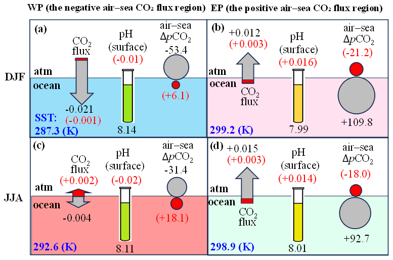
Figure 11 Schematic diagrams illustrate B–CTL (gray colors) and the differences between POP2–waves and B–CTL (red colors) in air–sea CO₂ flux (arrows), surface pH (tube colors indicator), and air–sea ΔpCO₂ (circle markers) over the oceanic CO₂ uptake region (WP; 160–180° E, 35–40° N) and the oceanic CO₂ outgassing region (EP; 230–250° E, 0–5° S). Each panel includes an ocean-atmosphere interface, with ocean color shading representing relative SST levels across different seasons. The lower-left corner displays the SST value, (a) WP in DJF seasonal mean, (b) EP in DJF seasonal mean, (c) WP in JJA seasonal mean, and (d) EP in JJA seasonal mean.

While the current POP2–waves framework highlights the importance of online coupling and ΔpCO₂-driven feedbacks, several avenues remain to future refine the model. A key priority is the continuous improvement of gas transfer velocity formulations. Future efforts will focus on transitioning to the new generalized formulation proposed by Deike et al. (2025), which incorporates updated coefficients and accounts for an asymmetric bubble flux contribution. While this advancement is expected to have a minor impact on oceanic CO₂ flux estimations, it holds potential significance for constraining global marine O₂ fluxes. Furthermore, moving toward a fully coupled Earth System Model (ESM) – which integrates dynamic atmospheric feedback alongside ocean and wave components – will be pivotal to better unravel the long-term impacts of wave-induced processes on global marine biogeochemical cycles.