Rapid Evaluation Framework for the CMIP7 Assessment Fast Track

As Earth system models (ESMs) grow in complexity and in volume of output data, there is an increasing need for rapid, comprehensive evaluation of their scientific performance. The upcoming Assessment Fast Track for the Seventh Phase of the Coupled Model Intercomparison Project (CMIP7) will require expeditious response for model analyses designed to inform and drive integrated Earth system assessments. To meet this challenge, the Rapid Evaluation Framework (REF), a community-driven platform for benchmarking and performance assessment of ESMs, was designed and developed. The initial implementation of the REF, constructed to meet the near-term needs of the CMIP7 Assessment Fast Track, builds upon four disparate community evaluation and benchmarking tools that are coupled together using the Coordinated Model Evaluation Capabilities (CMEC) framework. The REF runs within a containerized workflow for portability and reproducibility and is aimed at generating and organizing diagnostics covering a variety of model variables. The REF leverages well documented observational datasets to provide assessments of model fidelity across a collection of diagnostics. All diagnostics were identified and selected with community involvement and consultation. Operational integration with the Earth System Grid Federation (ESGF) will permit automated execution of the REF for selected diagnostics as soon as model output data are published on ESGF by the originating modeling centers. The REF is designed to be portable across a range of current computational platforms to facilitate use by modeling centers for assessing the evolution of model versions or gauging the relative performance of CMIP simulations before being published on ESGF. When integrated into production simulation workflows, results from the REF provide immediate quantitative feedback that allows model developers and scientists to quickly identify model biases and performance issues. After the REF is released to the community, its subsequent development and support will be prioritized by an international consortium of scientists and engineers, enabling a broader impact across Earth science disciplines. For instance, the REF will facilitate improvements to models and will enhance confidence in model projections through process-based selection of models based on their performance with respect to observations. Production of reproducible diagnostics and community-based assessments are key features of the REF. Furthermore, providing interoperability with existing evaluation packages assures that contributions from previous community efforts will be available for use in future model intercomparison projects.

1 Introduction

Earth system models (ESMs) are the primary tools for the scientific community to study interactions at a wide range of scales, from sub-daily to millennial, between the atmosphere, land, ocean, cryosphere, and biosphere, and how the Earth system responds to human-induced and natural forcings (e.g., Mauritsen et al., 2019; Séférian et al., 2019; Yukimoto et al., 2019; Boucher et al., 2020; Danabasoglu et al., 2020; Senior et al., 2020; Döscher et al., 2022). Currently, a new generation of ESMs is being finalized and new simulations will be generated for the Seventh Phase of the Coupled Model Intercomparison Project (CMIP7) and the precursory CMIP7 Assessment Fast Track. As the number of models, ensemble sizes, complexity and output requirements continue to grow, there is an urgent need to objectively evaluate the fidelity of these models and exploit the wealth of information they provide in order to efficiently advance our understanding of the Earth system and to inform climate mitigation and adaptation policies. This includes, specifically, identification of model uncertainties or systematic biases that may prevent us from objectively constraining model-derived projections of future climate change. Addressing this need requires developing efficient evaluation methods capable of making use of the growing archive of model output and reducing the time required to translate the output into meaningful scientific insight. The rapid growth of ESM data, driven by model complexity and computational advances, creates both opportunities and challenges. Effective, reproducible, accurate, and unbiased data processing is crucial for translating model outputs into actionable insights for climate policy (IPCC, 2023).

The CMIP Model Benchmarking Task Team (MB-TT) was created to address this challenge in preparation for CMIP7 and the contribution deadline for the Seventh Assessment Report of the Intergovernmental Panel on Climate Change (IPCC-AR7). Following the first phase of the MB-TT, which reviewed ESM evaluation and benchmarking approaches and identified the collection and collation of existing community benchmarking software packages (Hassler et al., 2026a), and outlined best practices for the use of observational datasets for model evaluation (Beadling et al., 2026); the MB-TT has now expanded its efforts toward developing a community-designed Rapid Evaluation Framework (REF) for routine and rapid benchmarking of CMIP simulations. The conceptual design of the REF was developed at an MB-TT workshop in May 2024 and approved by the CMIP Panel in July 2024, with development work commencing in October 2024. The initial design was strongly motivated by the ideas and vision developed for CMIP6 (Eyring et al., 2019); the goal of the REF for CMIP7 is to deliver a complete end-to-end system that will provide a high-level, systematic and rapid performance assessment of CMIP models, initially targeting the model experiments contributing to the CMIP7 Assessment Fast Track, which will support the IPCC-AR7 (Dunne et al., 2025). The vision of the REF is to be a community-owned evaluation framework, leveraging existing community-built model evaluation packages and incorporating an application programming interface (API) that will execute modules for generation of diagnostics and the metrics that underlie them.

Rather than directly ranking models, the REF is primarily concerned with providing objective measures of model performance to allow the wider community to make informed decisions about models that are most appropriate for their specific needs. This requires a standard set of diagnostics and performance metrics to facilitate the comparison of key variables simulated by models with standardized observational reference datasets, and assessment of whether fundamental processes in the Earth system are adequately represented in the models. Once expanded for community use beyond the initial Assessment Fast Track version, the REF will have a wider array of applications and users, including other modeling communities and scientific domains, as well as organizations utilizing CMIP models for conducting feedback analysis, impact assessments, or financial planning. To facilitate understanding of the descriptions of the REF, key terms used throughout the manuscript are defined here. This terminology may not be used consistently across all Earth science disciplines.

• Reference Dataset. A reference dataset is a collection of observationally constrained or model data used as a standard within a model evaluation diagnostic. Examples may include in situ measurements, extrapolated data (from statistical or AI/ML methods), remote sensing data, reanalysis products, or any other dataset that is meant to represent a best estimate of a geophysical quantity or a physical, chemical, biological, or ecological state or process.

• Model Variable. A model variable is any quantitative representation or characterization of a physical, chemical, biological, or ecological state or process that changes during execution of the model. Variables are used to represent mass, energy, velocity, momentum, flux rates, and other parameters within models. Model variables may or may not represent observable quantities, and they may be inferred, estimated, or calculated from other related variables or observables.

• Diagnostic. A diagnostic is a comparison of a model variable or some combination of model variables with a reference dataset or an intercomparison across models of a model variable or some combination of model variables (Hassler et al., 2026a). A diagnostic may also represent an evaluation of a relationship between multiple model variables and/or multiple reference datasets (i.e., Relationship Diagnostics). Diagnostics have sometimes been called “confrontations” since the objective is to confront models with best-available observations or with best-available model or model ensemble outputs. A diagnostic consists of one or more model performance metrics.

• Diagnostic Collection. A diagnostic collection is a grouping of one or more diagnostics for a given model variable, phenomena, or theme being evaluated.

• Metric. A metric is a single statistical evaluation contained within a diagnostic. A diagnostic may consist of more than one metric. Examples include bias, root mean squared error (RMSE), spatial or temporal correlations (Taylor, 2001), Earth Mover's Distance, Hellinger Distance (Hellinger, 1909), phase/timing of the seasonal cycle, amplitude of the seasonal cycle, inter-annual variability (Giorgi and Francisco, 2000). Not all metrics are useful for all variables or should be used with every observationally constrained dataset. Each metric may be evaluated to produce a metric scalar.

• Metric Scalar. A metric scalar is the numerical output resulting from the calculation of a performance metric (e.g., the calculated bias).

• Score. A score is a scalar value (0.0–1.0) transformed from a metric scalar or produced by aggregating multiple metric scalars or multiple scores together.

• Verification. Verification is the process of assessing model consistency in terms of correct implementation of the represented processes as expected from the model and simulation experimental design. Sometimes, this is accomplished as the model simulations are being produced (such as monitoring the conservation of total energy, total atmospheric mass, etc.), and the focus is often on the artifacts introduced by the numerical discretization scheme (e.g., Lauritzen et al., 2022) or by changes to software or hardware used for the simulations (e.g., the Ensemble Consistency Test in Baker et al. (2015) and the Time Step Consistency Test in Wan et al., 2017).

• Validation. Validation is the process of determining the degree to which a model accurately represents processes in the real world, particularly for the intended uses of the model. Validation can include a broad range of aspects from ensuring correct units and the sign of the data produced, to the interactions between model components or variables and process representations.

• Fidelity. The fidelity of a model is a quantitative assessment of the degree to which model output corresponds to the reference data in aggregate, resulting from a validation exercise. One approach for deriving a fidelity metric is to aggregate relevant scores.

2 Conceptual Design of the REF

2.1 Overview of the REF

The REF was designed to be a community-owned evaluation framework that leverages existing open source, community-built model evaluation and benchmarking packages that are integrated together through a standard application programming interface (API) that will execute modules for generation of diagnostics and the metrics that underlie them. By incorporating existing tools and metrics with publicly available reference datasets, the REF standardizes a community workflow for CMIP activities, reduces duplication of efforts for evaluating models, and, through deployment on the Earth System Grid Federation (ESGF), provides rapid feedback to the research community about relative model performance across a wide range of model components and variables. Moreover, the REF is expected to offer a starting point for the research community to expand model evaluation and benchmarking capabilities and applications within their own institutions or modeling centers.

The high-level workflow for the REF as it runs on ESGF nodes, as shown in Fig. 1, is triggered by the publication of new simulations requiring evaluation. After the model output has undergone a quality control check to assure the metadata are correct, data storage and compute resources are allocated for a new execution of the diagnostics generation process. As agreed upon by the CMIP Panel, model output that does not conform to the required Controlled Vocabulary (CV) and metadata standards will not be evaluated by the REF. Next, an optimized directed acyclic graph of tasks is produced, and processes are initiated to calculate model evaluation metrics and construct diagnostics. The outputs of diagnostics are then staged on public websites for sharing with the research community. The initial implementation of the REF was created to evaluate Assessment Fast Track simulations (Dunne et al., 2025), using five to six diagnostics across five Earth system realms with the expectation that additional diagnostics would be added in the future.

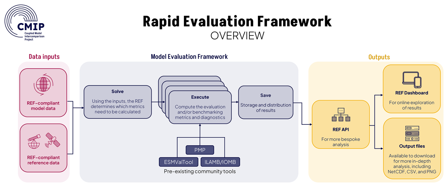
Figure 1 The high-level workflow for the Rapid Evaluation Framework (REF) run on Earth System Grid Federation (ESGF) nodes, shown here, combines quality-assured model output with a collection of observational reference data to initiate execution of relevant diagnostics and generation of tabular and graphical representations of a variety of metrics. The results are then published via an API for more bespoke analysis and on an online dashboard for community use. Obs is an abbreviation for observational, QA/QC is an acronym for Quality Assurance/Quality Control, and DAG is an acronym for Directed Acyclic Graph. Figure available at https://doi.org/10.5281/zenodo.15594501 (Hoffman et al., 2026).

Modeling centers usually evaluate their models during development with the overall performance documented and published once the models are finalized and key simulations are completed. However, this approach has three main limitations. First, the process is slow, and evaluation results often come too late to inform assessment reports or even later for stakeholders who need timely information. Second, these evaluation results are hard to access; they are scattered across different types of papers (technical or peer-reviewed, open access or not, etc.) across the modeling centers and often only partially included in IPCC reports, making them difficult to locate and piece together. Third, no consistent approach is applied across centers; each group runs its own evaluations using sometimes different methods, which makes comparisons between models difficult. The REF aims to address these issues by bringing together core evaluation frameworks and their diagnostic output in one place. This workflow is envisioned to help experts quickly assess, understand, and synthesize the performance of a new generation of ESMs for Assessment Fast Track simulations. The REF also makes it easier for stakeholders to access the information they need to support regional analysis for adaptation and mitigation, and it supports best practices for evaluation during model development. Running the REF before model output is submitted to ESGF offers modeling centers an additional option to systematically assess their models and to make targeted improvements during the development phase.

The REF aims to integrate well-documented reference datasets for comparison with model output. These reference datasets will be collected in obs4MIPs (Waliser et al., 2020), a project created to distribute data that support evaluation of ESMs via ESGF (nodes listed at https://esgf.github.io/nodes.html, last access: 3 August 2026). Obs4MIPs compiles a range of observationally constrained data, formatted according to CMIP conventions to ensure compatibility with model output. The published obs4MIPs datasets include variables such as temperature, precipitation, and sea level pressure, spanning various spatial and temporal ranges and scales across Earth system realms (Ocean & Sea Ice, Land & Land Ice, Atmosphere, Earth System, and Impacts & Adaptation), providing a comprehensive basis for model evaluation (Waliser et al., 2020). The formatting of obs4MIPs data adheres to the Climate and Forecast (CF) conventions (Eaton et al., 2024) and the CMIP metadata standards (Eyring et al., 2016). These conventions ensure that data are consistently structured, with uniform variable naming, units, and metadata, facilitating easy comparison across model outputs.

While obs4MIPs serves an important role in distributing observational datasets, the REF is flexible and designed to use additional reference data available in the required format. This adaptability allows for the incorporation of new reference datasets as they become available, or when specific needs arise, ensuring that the framework can accommodate a broad range of observational data. The REF leverages the attributes provided by datasets to automate the diagnostic generation process. This automation requires standardization and coherent attributes across models, variables and experiments in order to correctly combine different datasets without manual selection by humans. Reference data used by the REF may span different time periods, a key point that analysts need to consider when interpreting the results of the available diagnostics. Moreover, community activities like CMIP should strive to ensure that reference data span the full contemporary time period of simulation experiments intended to reproduce recent historical trends and variability. The REF does not aim to reformat reference or model data, and REF users must ensure the data they wish to use follow the CF conventions and meet the CMIP metadata standards to be considered REF-compliant data (Fig. 1). Quality checks (Hassler et al., 2026b) are required to assure the data used for evaluation and benchmarking diagnostics are consistent and reliable, enabling meaningful model-data comparisons (Hawkins and Sutton, 2016). These quality checks do, in some cases, go beyond the checks required for data publication to ESGF.

2.2 Community Engagement

Key stakeholders for the co-development of the REF were identified as modeling centers involved in the Assessment Fast Track, reference dataset providers, evaluation tool and package developers, diagnostic developers and climate scientists, including IPCC authors, seeking to analyze the Assessment Fast Track output. The MB-TT initiated work on the REF based on the results of the CMIP6 Community Survey (O'Rourke, 2025), conducted by the World Climate Research Programme (WCRP) from January to March 2022. Detailed analysis of the survey results by the Task Team (Lee, 2024) revealed calls for open and transparent model benchmarking and evaluation and the ability to run CMIP evaluation tools alongside ESGF, as part of the data publication process, with provision of evaluation results display.

Members of Fresh Eyes on CMIP worked with the CMIP-International Program Office and the MB-TT to develop a survey that was circulated to modeling center science and technical leads, as well as more widely in the Fresh Eyes on CMIP and CMIP community mailing lists and via social media. The survey was open 7–17 May 2024, and generated 152 unique responses, and the responses were analyzed by members of the Fresh Eyes on CMIP and reported at a MB-TT workshop. These survey results informed design and development of the initial REF proposal. Suggestions included considering multiple software tools, strategies to ensure accessibility, tools for quality control, and transparency and provenance for reference datasets and model output. Additional suggestions included acceptance of data not processed by the Computer Model Output Rewriter (CMOR; Taylor et al., 2004), potentially with AI-assisted reformatting, improved accessibility through use of ESGF and cloud-based computing to enhance data inclusivity and flexibility, as well as errata tracking. A detailed analysis of the survey results is available in the survey report by Wang et al. (2025).

A separate community survey was subsequently disseminated to modeling centers in June 2024 that included requests for input on evaluation tools used, interest in use of a benchmarking framework within their own computing environments, and willingness to submit preliminary model output for quality assurance and control checks (O'Rourke, 2024). This survey informed refinement of the framework structure and implementation plan. In September 2024, a survey was disseminated to modelers, modeling centers, and reference dataset and data infrastructure providers, requesting input regarding the specific diagnostics that should be prioritized for inclusion in the REF, receiving 53 responses. A co-development session with members of the Earth observation community was held at the European Space Agency (ESA) Climate Change Initiative (CCI) and Climate Modelling User Group (CMUG) integration meeting in October 2024, which resulted in the inclusion of ozone-related metrics in existing diagnostics where appropriate and two additional cloud diagnostics. The outcomes of the survey, in combination with suggestions from the MB-TT, resulted in a set of diagnostics, shown in Sect. 4 and published separately (CMIP Model Benchmarking Task Team, 2026b). The REF was thereby launched on 4 November 2024, at a community-engagement event that saw wide participation. Successive months were dedicated to implementation of the diagnostics from four existing evaluation and benchmarking packages within the REF architecture. The packages selected for providing diagnostics for the Assessment Fast Track REF were ESMValTool, PMP, ILAMB, and IOMB, which are described below in Sect. 4. During this period, engagement efforts focused on technical implementation, involving members of the community responsible for provision of supporting infrastructure and quality control, including the WGCM Infrastructure Panel (WIP), obs4MIPs Steering Panel, the ESGF-WIP Quality Assurance and Control Working Group, the CMIP Data Request and CVs Task Teams, as well as the IPCC Task Group on Data Support for Climate Change Assessments (TG-Data), on their citation and provenance requirements for the REF, see Sect. 4.6.

A preliminary prototype of the working suite was stress-tested for operational usage in time for the REF Hackathon, which was held at the Met Office, in Exeter, UK, from 10–13 March 2025, and included dedicated drop-in sessions for modelers and reference dataset providers. This prototype was able to ingest a sample of CMIP6 model output and obs4MIPs data, running a small subset of ILAMB, PMP, and ESMValTool diagnostics. In May 2025, modeling center science and technical personnel, as well as previous attendees of the REF launch, were invited to attend the launch of the beta version of the REF. Approximately 107 participants registered for the demo and to attend follow-up feedback sessions in June 2025 regarding the beta release. This beta testing period was instrumental for building an easy-to-use tutorial and documentation, solving potential issues with REF usage on HPC machines, and receiving feedback from users, with the aim of delivering a public release of the REF for actual usage with Assessment Fast Track outputs in October 2025.

3 Target Applications

Considering the REF scope, stakeholder consultation and initial implementation plan for the Assessment Fast Track simulations, three primary potential applications for the REF were identified: provide information about scientific performance of ESMs to stakeholders and policymakers, focus on key sensitivity indicators, and enhance equality in model data access. The primary application of the REF is to provide stakeholders from the data analysis and impacts assessment communities with timely information about the scientific performance of ESMs with respect to observationally constrained (reference) datasets across all Earth science realms (Atmosphere, Ocean and sea ice, Land and land ice, Earth system, Impacts and adaptation). Reference data are available primarily but not exclusively from the contemporary observational period, approximately over the last 50 years. Secondarily, the REF produces diagnostics focused on key sensitivity indicators that typically do not have corresponding observational constraints, such as equilibrium climate sensitivity (ECS) and transient climate response (TCR). Access to all of this diagnostic information assists stakeholders in selecting simulation results for further analysis, downscaling studies, impacts analyses, or other research. Moreover, the results of the REF can increase equality in climate data access for community members who lack adequate computer resources or Internet access. In some cases, diagnostics from the REF include graphs, charts, or figures that can be used in research publications or assessment reports, offering analysts more time to focus on specific research questions that may use information from the REF.

A key design goal of the REF is that it can be used by modeling centers, research institutions, and individual scientists to enable validation of ESM output prior to publication of simulations on ESGF, intercomparison of model results, and general purpose analysis. Running the REF prior to data submission provides the opportunity for data providers to gauge the performance and sensitivity of their simulations in a standard fashion at any time. Modeling centers typically use their own collections of diagnostics, often developed in-house, for routine model assessment, while other centers or institutions have adopted community-developed evaluation tools or employ a combination of community tools and in-house diagnostics. The REF offers a general purpose framework for model evaluation and is equally useful for tracking the scientific performance of different versions of the same model. The REF diagnostics also provide a convenient means for determining if model changes during development yield improvements. Thus, modeling centers may find that running the REF as a part of their workflow for repeated simulations provides a practical way to track evolving performance of their model. It may also be necessary to reformat the relevant model output variables for each simulation, making them CF-compliant and ensuring CMIP naming standards and metadata are provided, within the workflow for the REF to be able to run correctly. Moreover, analysts from different research communities may want to add functionality to the initial REF implementation to enable use of other observational datasets, additional diagnostics, and other metrics as discussed in Sect. 5.5.1.

Furthermore, the REF could serve as an early warning system for modeling centers to identify inconsistencies in the model variables in a more complex way than was done for the prior CMIP activities (e.g., Taylor et al., 2004) and thus reduce ESGF data traffic and storage of erroneous data, limiting data use by the wider community. The REF can also be used for a variety of model intercomparison activities outside of the scope of CMIP, and project leaders can ask simulation contributors to run the REF and provide standard diagnostic results instead of sharing large volumes of model output. Additionally, the REF enables individual researchers interested in Earth system science to explore model output and apply well documented reference data to better understand model capabilities and gaps in process representation. The REF provides a standard framework for integrating additional diagnostics for use by research institutions or local analysts and scientists. New diagnostics integrated into the REF can be easily shared amongst modeling centers and researchers, and they become key candidate additions to future public releases of the community version of the REF.

4 System Description of the CMIP7 Assessment Fast Track REF

4.1 Included Evaluation and Benchmarking Packages and the Coupling Strategy

The open source evaluation and benchmarking packages described below – ESMValTool, PMP, and ILAMB & IOMB – were chosen for inclusion in the first version of the REF because they are open source, were relatively mature packages at the time, and combined, they permit comprehensive model evaluation across all the atmosphere, ocean and sea ice, land and land ice, Earth system, and impacts and adaptation realms. Subsets of diagnostics from each package were selected based on input from the MB-TT and the community. For the initial version of the REF, diagnostics were restricted to analyze only monthly mean output from the expected new simulations. In this section, the packages are briefly described, although a more in-depth description of them can be found in Hassler et al. (2026a), and the Coordinated Model Evaluation Capabilities (CMEC) standards are also described, since they offer a strategy for integrating these disparate evaluation packages.

4.1.1 ESMValTool

The Earth System Model Evaluation Tool (ESMValTool) is an open source community-developed software package aimed at computing many different diagnostics and metrics for the evaluation and benchmarking of ESMs (Righi et al., 2020; Eyring et al., 2020; Lauer et al., 2020; Weigel et al., 2021; Schlund et al., 2023; Lauer et al., 2025; Schlund et al., 2025; Andela et al., 2025). Many of the diagnostics and metrics that have been officially released in ESMValTool have been systematically used for the production of multi-model intercomparisons embedded in several chapters of Working Group I (WGI) of the IPCC Sixth Assessment Report (AR6) (IPCC, 2023). ESMValTool strongly advocates traceability and reproducibility; therefore, all diagnostic results are provided with metadata documenting the provenance of the model output and reference data, the software packages used, and the calculated metrics and diagnostics. The software package also deals with the adjustment of model or observational datasets that are not strictly compliant with the CF conventions. Although the core capabilities of ESMValTool are fully Python-based, diagnostics can be based on other open source languages such as NCL (NCAR Command Language) or R. For all contributions, ESMValTool implements rigorous technical and scientific reviews before new code can be included in the official release, requiring Python Enhancement Proposal (PEP) 8 standards, and testing with pre-commit and Codacy for maturity of the code and standardization.

4.1.2 PMP

The PCMDI Metrics Package (PMP) is an open source Python software package developed for objective and rapid assessments and benchmarking of ESMs, against the most up-to-date observational datasets (Lee et al., 2024). The PMP has played an important role in the systematic evaluation of many simulations across CMIP generations, with a strong emphasis on physical climate metrics, particularly atmospheric means and variability. Among its diverse suite of metrics, a subset of metrics that are calculated based on the monthly time series of model variables were chosen for the first implementation in the REF (Table 1). This subset of metrics includes the annual cycle of different atmospheric variables (Gleckler et al., 2008), El Niño Southern Oscillation (ENSO), CLIVAR (Climate and Ocean: Variability, Predictability and Change) metrics (Planton et al., 2021), extra-tropical modes of variability (Lee et al., 2021), and global monsoon metrics (Wang et al., 2011). By offering a database of pre-computed statistics for CMIP6 models, the PMP streamlines the comparison process, making it easier for modeling centers to evaluate their results against established benchmarks.

4.1.3 ILAMB and IOMB

The International Land Model Benchmarking (ILAMB) and International Ocean Model Benchmarking (IOMB) are open source Python software packages that share a large portion of the same codebase. They were developed to provide systematic assessment of land and ocean model performance, primarily for terrestrial and marine biogeochemistry, through comparison with reference datasets (Collier et al., 2018; Luo and Hoffman, 2022; Fu et al., 2022). Diagnostics and metrics within ILAMB and IOMB were developed with engagement of land and ocean modelers and with the in situ and remote sensing observational communities (Luo et al., 2012; Hoffman et al., 2017). Both packages were used to evaluate and intercompare historical simulations from CMIP5 and CMIP6 (IPCC, 2023, Chap. 5, Fig. 5.7), as well as serving important roles in informing the development of land and ocean components for DOE's Energy Exascale Earth System Model (E3SM; Burrows et al., 2020; Zhu et al., 2019; Yang et al., 2019) and the Community Earth System Model (Lawrence et al., 2019). ILAMB and IOMB both offer a variety of statistical metrics, including bias, RMSE, timing/phase of the seasonal cycle, spatial correlation, and interannual variability. Scores from these metrics are aggregated to provide high-level scores for each model-dataset pairing. Functional relationship metrics within ILAMB and IOMB evaluate the degree to which model variable-to-variable relationships correspond to those of observational data. For example, the relationship between gross primary production (GPP) and mean annual temperature in the model should correspond well with the same relationship extracted from observational data. ILAMB and IOMB produce hierarchical webpages designed to offer users and analysts the ability to view many metrics at once for a given model-dataset pair, as well as to intercompare graphical representations of metrics across all models at once.

4.1.4 CMEC

Coordinated Model Evaluation Capabilities (CMEC) is an effort to bring together a diverse set of analysis packages that have been developed to facilitate the systematic evaluation of ESMs (Ordonez et al., 2025). CMEC provides the strategy for coupling multiple community benchmarking packages in the REF. CMEC includes capabilities supported by multiple agencies, and capabilities that have been contributed by community-based experts and international agencies. With widespread and rapid growth in the number of available diagnostic and model evaluation tools, a lack of standards within the evaluation community have meant that running even a single evaluation tool can require extensive user intervention. Given the significant commonality in how these evaluation tools operate, interoperability is a natural goal achievable through robust and light-weight standards. The three goals of the CMEC project include: (1) to develop robust and light-weight standards for the operation of evaluation packages and their output; (2) to develop accompanying tools for installation of evaluation packages, coordinated execution of evaluation packages, and obtaining data products necessary for operation of these tools; and (3) to build connections across groups, research centers, and individual investigators performing model evaluation. The CMEC standards were adopted for integrating the output of diagnostics produced by the model benchmarking packages described above.

4.2 Diagnostics

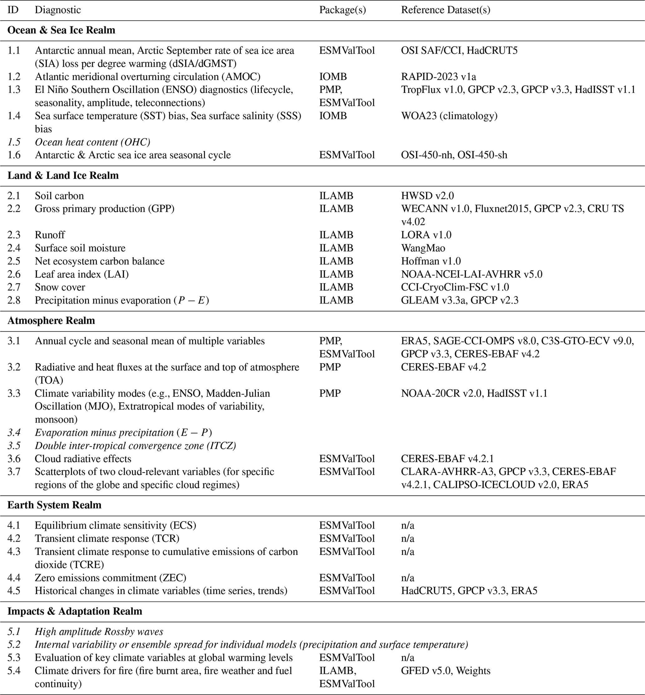
At the heart of the REF are the diagnostics that were selected in an iterative process (see Sect. 2.2) that can be calculated with each new simulation that is presented to the REF. The diagnostics are grouped according to the five different realms that were identified for the CMIP data request and each diagnostic included in this first version of the REF is calculated by only one software package. Table 1 provides an overview of all the diagnostics that were selected for the first version of the REF, based on the diagnostics table published on Zenodo (CMIP Model Benchmarking Task Team, 2026b), their realm, the software package with which the diagnostic is calculated, and the reference datasets used in the comparison. A more detailed table of the diagnostics is presented in Appendix B. For some of the diagnostics, different methodologies adopting different software packages across the diagnostic providers were discovered (e.g., double Inter-tropical Convergence Zone (ITCZ) biases); in this case, the principle of minimal computational resources and least number of required variables was adopted in order to choose the appropriate tool to be responsible for the diagnostic in the REF.

Table 1 Based on community recommendations, an initial set of diagnostics was selected, published at https://doi.org/10.5281/zenodo.20175394 (CMIP Model Benchmarking Task Team, 2026a), for incorporation into the initial version of the REF for evaluating relevant CMIP7 Assessment Fast Track simulations. Diagnostics 1.5, 5.1 and 5.2 are listed in italic style text because they were not implemented for the initial version of the REF. Diagnostic 3.4, shown in italic text, was replaced by 2.8 for the Land & Land Ice realm, and 3.5, also shown in italic text, is available as part of 1.3 and not separately.

n/a – not applicable.

During the REF development phase, it became clear that two of the identified diagnostics were not available from the software packages implemented in the Assessment Fast Track REF. These diagnostics, with their unique IDs, 5.1 (High amplitude Rossby waves) and 5.2 (Internal variability or ensemble spread for individual models), were then removed from the list of those to be integrated in the initial REF version, following consultation and agreement from the Impacts & Adaptation CMIP Data Request Author team leads and co-chairs of the Vulnerability, Impacts, Adaptation and Climate Services (VIACS) Advisory Board. One additional diagnostic was removed from the diagnostic list, ID 1.5 (Ocean heat content (OHC)), since also for this diagnostic no code for its calculation was available from the software packages. The original diagnostics ID 3.4 (Evaporation minus precipitation (E−P)) was moved to a different realm (now ID 2.8 (Precipitation minus evaporation (P−E))), and diagnostic ID 3.5 (Double inter-tropical convergence zone (ITCZ)) was added to another existing diagnostics (ID 1.3 (El Niño Southern Oscillation (ENSO) diagnostics (lifecycle, seasonality, amplitude, teleconnections))) to better reflect the actual calculated metrics.

A more detailed description of each diagnostic and the rationale and methodology for its implementation is presented in Appendix C.

4.3 Data Request Opportunity

For CMIP7, the data request to modeling centers is based on different “opportunities” that the community could submit to the CMIP IPO, following a community-wide call, each focusing on a specific scientific topic. Each opportunity contains a concise description of its scientific goals and a list of all model variables that are requested from simulation output to achieve these goals. The different data request opportunities are grouped according to five realms (Ocean & Sea Ice, Land & Land Ice, Atmosphere, Earth System, and Impacts & Adaptation), which are the same as those that were used as a basis for selecting REF diagnostics (see Sect. 4.2).

An opportunity regarding the REF was submitted to the Data Request Task Team's open call to ensure that the model variables required by the REF for generating the REF diagnostics were clearly identified and that modeling centers wishing to use the REF with their simulations would have a checklist of model variables needed for producing the REF diagnostics. While some REF diagnostics use only a single model variable from the historical simulation, others require two or more model variables from multiple different simulations, as described in the definitions in Sect. 1. Since the REF diagnostics span all five data request realms, a variable group request was submitted for each realm. The variable groups combined form the “REF CMIP7 data request” opportunity. The opportunity was published as part of the v1.2.1 release of the data request, consisting of five variable groups, containing 80 variables in total. Many of the variables are from the recently developed list of baseline climate variables for Earth system modeling (Juckes et al., 2025), which is a subset of variables reflecting the most frequently used elements of CMIP6. To facilitate finding information about the REF opportunity in the different data request documentation papers, it was decided that each paper would contain a very brief description of the opportunity and refer to the documentation paper about the atmosphere realm, where a more detailed REF opportunity description was added (Dingley et al., 2026).

4.4 Observations

Observations play a key role in the REF and several diagnostics require observed quantities for different climate variables across domains for model evaluation. For each diagnostic, we have identified at least one reference dataset for inclusion in the REF (see complete list in Appendix A). To ensure compliance with the Findability, Accessibility, Interoperability, and Reusability (FAIR) data standards (Wilkinson et al., 2016), all observational datasets included in the REF are required to have a fully open access license (e.g., CC-BY-4.0, CC0, OGL) and follow the CF conventions (Davis et al., 2024) to ensure technical alignment with CMIP standard output. This is enabled by making the datasets available for downloading on ESGF servers (Cinquini et al., 2014) as part of the obs4MIPs project (Gleckler et al., 2011; Teixeira et al., 2025; Ferraro et al., 2015; Waliser et al., 2020). For any datasets not meeting the open access criteria, the REF Delivery Team obtained a relaxation of the license constraint by formally requesting and receiving agreement from individual dataset providers. Observational datasets for the REF were then processed in compliance with the obs4MIPs Data Specifications 2.5 (ODS2.5) (Gleckler et al., 2024) with approval from the obs4MIPs Steering Panel (OSP). In facilitating observational data ingestion for the REF, two additional criteria not fully addressed by the ODS2.5 specifications were identified, for which the REF delivery team has drafted guidelines. These criteria relate to the treatment of uncertainty information in the data and for the formulation of complex citations (see discussion in Sect. 4.5 and 4.6). In an effort to recognize the need for observational record lengths to be as closely aligned with CMIP simulations as possible, we specify that observational datasets should be available at least until the end of 2016, ensuring that the data is less than five years out of date with historical simulations from CMIP7, that run until the end of 2021. We consider the availability of data towards the end of the historical simulation period to be important for the calculation of certain statistical properties such as trends used in evaluation. Where the observational datasets currently do not meet this requirement, we have highlighted such entries in Table A1 in Appendix A, so that the data sets may be extended or replaced as appropriate in the future.

Two pathways were identified for observational dataset providers to submit their datasets for future inclusion in the REF. The first step in both cases is to submit a dataset proposal to obs4MIPs for approval by the OSP, which can either be done directly by the dataset provider or via a third party with permission from the dataset provider. Once the dataset has been approved by the OSP, the registered content, including the dataset name, version, data provider details and release date should be submitted to the Program for Climate Model Diagnosis and Intercomparison (PCMDI) obs4MIPs CMOR Tables repository (https://github.com/PCMDI/obs4MIPs-cmor-tables, last access: 3 August 2026). This process provides the dataset with a unique source_id, following CMIP conventions. Datasets can then be prepared for compliance in one of two ways:

• using the CMOR software as advised by the OSP to prepare their dataset, following instructions and examples on the PCMDI obs4MIPs CMOR GitHub repository (the “CMOR pathway”).

• using software packages such as ESMValTool to generate CMOR-like datasets that have additional scripts ensuring CMOR and obs4MIPs compliance (the “CMOR-like pathway”).

The CMOR pathway intrinsically provides a form of validation for datasets before publication through the use of the CMOR software. As the CMOR-like pathway may not provide the same level of validation, the REF Delivery Team has developed a validation script that the prepared CMOR-like datasets must pass before publication. The prepared datasets are then published to ESGF via one of the two Assessment Fast Track REF nodes, at the Center for Environmental Data Analysis (CEDA, United Kingdom) or at Oak Ridge National Laboratory (ORNL, United States of America).

For certain diagnostics (1.1 and 5.4 in Table 1), the reference datasets listed in Table 1 are pre-processed to produce one or more static files with information needed for the diagnostic. In such instances, these files are stored internally within the corresponding diagnostic package, and the REF includes acknowledgments and references for the input datasets used to produce the files. For such exceptions, the input datasets themselves are not required to be published on ESGF.

4.5 REF Requirements in Addition to obs4MIPs Compliance – Treatment of Uncertainties

Currently, most diagnostics within the REF do not incorporate uncertainty information from reference datasets. Where available for a reference dataset used in the diagnostics, the standard error of the mean or upper and lower bounds around the mean are used. Future plans for the REF include using multiple reference datasets to account for observational uncertainty as seen commonly in the literature. The unavailability of comprehensive and accurately characterized uncertainty information with the observational data was identified as a key barrier to incorporating this information by diagnostic developers. Feedback from observational data providers indicated that any associated uncertainty and instructions on how to correctly apply such information is best provided by the data providers themselves. This prompted the REF Delivery Team to develop guidance for including uncertainty information in observational datasets; which was necessary to allow ingestion of uncertainty information by the REF. The initial proposal, originating from community engagement at the REF Hackathon with observational dataset providers and metrics package developers, was refined following consultation with the OSP and the CMIP-CVs Task Team. For the CMOR pathway, the following requirements are outlined:

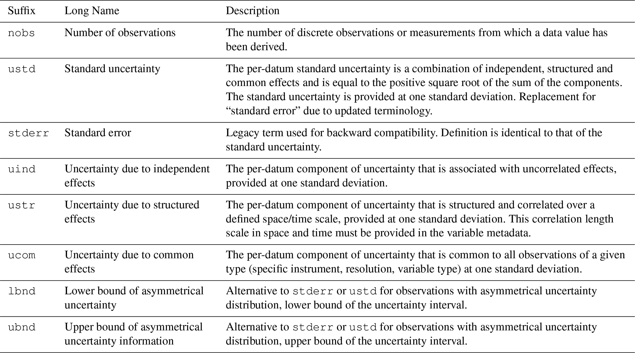
• All additional uncertainty information (see Table 2 for currently accepted information on uncertainty) is provided in a separate file. Initially, between one and three additional files will be used, depending on the extent of uncertainty information provided.

• The netCDF file containing the main geophysical variable has the global attribute has_aux_unc, and is set to TRUE when additional files containing uncertainty information are provided. It should be set to FALSE when no uncertainty information is provided. If this attribute does not exist, the REF will assume there is no uncertainty information provided to ensure back-compatibility with datasets already published through obs4MIPs.

• If has_aux_unc is set to TRUE, the netCDF file containing the main geophysical variable must have the global attribute aux_uncertainty_id. This contains all additional variable_ids for the uncertainty information provided, in the form of a string with spaces as delimiters.

• The CMIP global attribute, variable_id (as defined in Taylor et al., 2026), in the file containing the uncertainty information corresponds to variable name + accepted suffix (no separator between body and suffix). For accepted suffixes, see Table 2.

• Variable name within the netCDF file corresponds to the variable_id.

• A technical note including detailed explanation of additional uncertainty information, is provided for each dataset following guidance in Hegedűs et al. (2025).

This distinction between how uncertainty information may be included in CMOR and CMOR-like datasets is due to the current capabilities of the CMOR software. Currently, CMOR does not accommodate the addition of ancillary variables in its output, and the required software update for inclusion is not feasible within the Assessment Fast Track REF timeline. For the CMOR-like pathway, there is no requirement to add the uncertainty information in separate files. Instead, additional uncertainty fields may be provided following CF conventions, by adding them as ancillary variables in a netCDF-CF file. The additional global attributes has_aux_unc and aux_uncertainty_id are still required, and the variable_id should be constructed as described above only using the suffixes from Table 2. This guidance was developed as a basic framework to enable the community to utilize a wider range of uncertainty information during the development of REF diagnostics.

Table 2 Suffixes for the variable_id were proposed to describe the uncertainty information included with the reference datasets.

4.6 REF Support of IPCC-AR7 Related to the Enhanced Traceability of its Results – Complex Citation

The REF Delivery Team consulted with the IPCC Task Group on Data Support for Climate Change Assessments (TG-Data) on their citation and provenance requirements for the REF. The IPCC TG-Data aims to enhance the traceability of key results presented in the AR7 (AR7; Stockhause et al., 2024) cycle using the new Complex Citation standard (Agarwal et al., 2025) for documentation and standardized provenance records for gathering the required information. This simple but flexible Complex Citation approach allows for the traceability of data product generation and the citation of multiple datasets or data subsets in a single referenced object called Complex Citation Object (CCO). TG-Data aims to include CCO references in every figure caption of the AR7. Prerequisite to this is the provision of detailed information on input data usage in the form of persistent identifiers (PID) for each file and each citable entity.

The REF has identified the need for the reference datasets to be published on ESGF with their Handle IDs and data collections with their DOIs. ODS2.5 already requires each file to have a global attribute called tracking_id used as PIDs on ESGF, a unique identifier with prefixes specified for each ESGF project. In addition, reference datasets used by the REF also require the inclusion of the DOI as a global attribute to ensure compatibility with CCO. The REF leads the task of defining a provenance template for authors of the IPCC AR7 as guidance on providing the CCO-related information.

Through the CMIP7 data citation, the CCO captures provenance information at the granularity of a model's contribution to an experiment. The list of the file handles of the specific data that were used from within the CMIP7 citation resource provides traceability.

4.7 Technical Implementation

The REF workflow consists of four steps:

• Ingestion: The user registers the source datasets that can be used (reference data and model output). The associated metadata is extracted and added to a local database along with the respective file paths. Only ingested files are used in any execution calculations.

• Solve: For each diagnostic, the possible executions that would be required are determined using the data requirements of a metric and the catalog of datasets that have been ingested. A hash of the datasets required for each execution is stored in the database and subsequently used to determine if a new execution is required or has already been performed.

• Execute: The executions that require running are then executed. The REF supports four key methods for executing diagnostics: Local-Serial, Local-Parallel, Celery and via an HPC Scheduler such as Slurm or PBS. The ESGF deployment uses the Celery-based executor, which runs diagnostics out-of-process and in parallel. Once the execution is complete, the CMEC-based outputs are parsed and any scalar value or diagnostic figures are added to the database for later display and use.

• Visualize: The results are then made available via a REST API (Representational State Transfer Application Programming Interface) and Typescript-based frontend. Python-based tooling may be developed in future releases to interact with the results, but is not currently implemented. The Frontend allows users to see the diagnostics that have been executed and the corresponding results. This includes the ability to track which datasets were used for a given execution, and the ability to download generated figures, datasets and log output. In some instances, the REF may also provide additional summary statistics across all executions for a diagnostic such as box and whisker plots.

4.8 ESGF Deployment

Figure 2 shows how the key services for the REF are integrated within the ESGF deployment. At the core of this system is the Compute Engine, which orchestrates the workflow by managing data ingestion and processing tasks. The Compute Engine manages a database (PostgreSQL or SQLite) of all the datasets, executions and results that have been performed. The Compute Engine will ingest new data when they become available either via consuming newly replicated events from the ESGF-Next Generation Event Stream, a Kafka-based service, or by periodically checking for newly available datasets. A “solve” is then be performed to determine if any new executions are required. For the ESGF deployment, each of the services (blue boxes in Fig. 2) are deployed as a Kubernetes service.

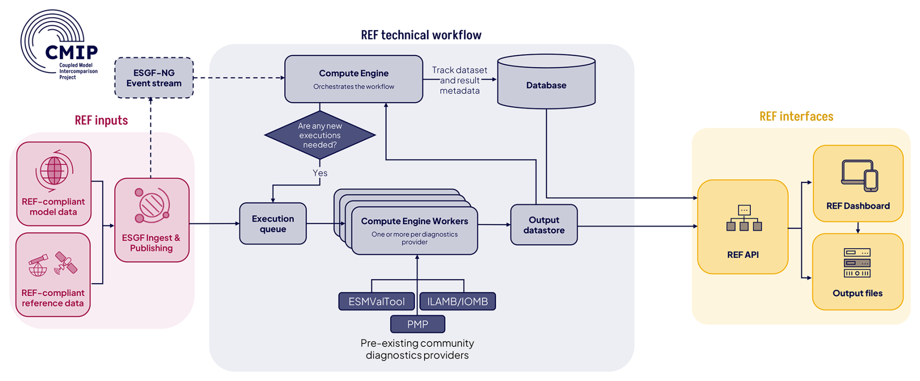
Figure 2 This detailed workflow diagram identifies key services provided by the REF and their relationships with external services and off-the-shelf components for the ESGF deployment. Figure available at https://doi.org/10.5281/zenodo.15595005 (Lewis et al., 2026b).

Data processing is handled by the Compute Engine Worker, which pulls executions from a queue and then executes the appropriate diagnostic. Each diagnostic provider is deployed as a separate service that can be scaled independently according to demand. This might be particularly important if one of the execution services requires more computational resources than the others. These workers require access to shared read-only mount containing input data (CMIP and observation datasets) and a mount for the Scratch Datastore where results are stored.

The Compute Engine watches for the success/failure of the executions on the workers. A subset of results are copied to the Output Datastore by the Compute Engine. During this process, metadata about the results are extracted into the database, including metric values, figures and data files. The use of a central database of results allows for efficient querying in the API across executions. This is critical to enable the ability to make dynamic data requests in the API. Users can access the REF through two primary interfaces: by directly querying the Data API, and the Portal, which consumes the Data API and serves as the landing page for information about the REF and provides synthesized results.

The REF can be deployed without the need for Kubernetes or docker depending on the constraints of the deployment target. Non-ESGF deployments will look very similar except that the ingestion and solving is performed via the Command Line Interface (CLI). The CLI is used to manually interact with the REF and its database, and is how users interact with the REF in a small deployment.

4.9 Prerequisites for Use

The REF operates on CF-compliant netCDF model output and reference datasets aligned with CMIP CV. When run within ESGF deployments, the REF is not be required to evaluate simulations that fail to meet required data-quality standards; if simulations cannot be processed by the REF, these simulations will be flagged or excluded from the public dashboard. The REF automatically accesses published model output and reference data; however, the REF also supports the analysis of datasets that are not published on ESGF, which allows modeling centers and individual researchers to perform their own model evaluations. A deliberate decision was made to enable the evaluation of datasets and model output that do not conform with the CMIP CV, enabling assessment of model versions not intended to be published on ESGF. In such offline cases, the local datasets must be available to all of the execution services, and ideally should have undergone a quality control (QC) process to assure that the metadata are correct and the data represent the desire output in the correct units.

The REF is designed to run on a variety of hardware platforms, from desktop computers to high performance computing (HPC) environments, and can be run either within virtual Conda environments or within Docker containers. Depending on the use case, either may be used; however, Docker containers are recommended for a production deployment, as they can be scaled independently. The instructions for installation and getting started are available via the REF documentation site at https://climate-ref.readthedocs.io/en/latest/ (last access: 12 June 2026) or the GitHub repository at https://github.com/Climate-REF/climate-ref (last access: 12 June 2026) (Lewis et al., 2026a).

5 Discussion

5.1 Community Co-development of a Framework

The REF Delivery Team was composed of an international team that brought together three different evaluation package providers, each of which possessed their own workflows, assumptions, and conventions. An independent delivery team leader was chosen to coordinate the development and architect the end-to-end workflow. Significant time was invested in identifying commonalities among the providers with the goal of minimizing the amount of additional development needed to integrate all the selected diagnostics into the REF. These tools were never designed to be interoperable and have long-standing communities that use the packages outside of the REF, so a requirement for minimal changes to the underlying packages was also mandated. Developing the appropriate abstractions and common language within the REF depended upon ongoing discussions and often required the prototyping of multiple potential solutions.

The REF system can be quite complex since it is composed of multiple services. A key requirement for the framework was to make it easy for additional packages to be integrated into the REF, both now and in the future. Care was taken to ensure that the amount of context that must be understood for a package developer to contribute diagnostics was kept to a minimum. The decision for the structure of the framework has two impacts, it provides a separation of concerns and minimizes the complexity required simply to contribute diagnostics, as well as providing the scope to support the different assumptions made by different providers. The ability to quickly refactor and modify the interfaces between the packages was critical. The use of a monolithic repository, where all of the REF-related packages were in a common GitHub repository with issue tracking and a Kanban board, was crucial for development and testing. Additionally this structure was important to enforce the need for type hints throughout the code base and providing high test coverage. The REF is openly developed and available on GitHub at https://github.com/Climate-REF/climate-ref under the Apache License 2.0 open source license. The version of the REF contemporaneous with the submission of this manuscript is archived on Zenodo at https://doi.org/10.5281/zenodo.15103441 (Lewis et al., 2026a).

The REF Hackathon, hosted by the UK Met Office in Exeter in March 2025, was convened to bring together the REF Delivery Team and to solicit early feedback from potential users. The Hackathon successfully accelerated code development and reference data conversion, obtained feedback and facilitated discussions about approaches for computing diagnostics and supporting traceability for CCO, and tested an alpha version on the UK Met Office HPC facilities. The Hackathon was held relatively early in the project development lifecycle and significant time was spent workshopping the conceptual framework of the REF. After the Hackathon, the research community continued to offer ideas for additional capabilities that could be enabled by the REF framework. A CMIP6-ready version of the REF was subsequently launched at the ESM2025 Final General Assembly on 7 October 2025. It was then further refined based on user feedback and the CMIP7-read version was launched at the CMIP 2026 Community Workshop held in March 2026 in Kyoto, Japan.

5.2 Key Reflections from the CMIP Panel

The CMIP Panel initiated the MB-TT, with a call for members in November 2022. The intention of the Task Team was to put together a group of experts who would work together to provide a systematic, open, and rapid performance assessment of the expected large number of models participating in CMIP7, providing a set of informative diagnostics and performance metrics. The Task Team originally focused on assessing evaluation approaches and software packages. However, it then became apparent that there was a larger opportunity here to fully integrate evaluation tools into the CMIP publication workflow with diagnostic outputs published alongside model output on ESGF and results displayed on an easily accessible website.

The REF became an extremely attractive option to the CMIP panel as it enables (1) consistent assessment of CMIP output by modeling centers, (2) support for author teams in the context of the IPCC and other national climate assessments and (3) input for model selection for downstream applications. The modeling centers are essential to the CMIP endeavor, so having a tool that supports their activities is the most important factor. Many of the CMIP panel members have contributed to IPCC assessments or national climate assessments, so it was clear that there was an opportunity to support such reports if model diagnostics were easily available to authors (reducing the workload of both authors and chapter scientists). Wider community discussions facilitated by the CMIP panel have also revealed enthusiasm from users of CMIP output for regional downscaling and impacts applications. The REF allows to have the diagnostics quickly available to support the choice of a limited selection of climate model output to serve their particular application.

The CMIP Panel view the REF as a potential game changer for users of CMIP data. CMIP Panel co-chair Helene Hewitt reflected, during opening remarks at the March 2025 Hackathon on-boarding session, that “as someone that was a Coordinating Lead Author of the IPCC AR6 WGI, I saw how much work our chapter scientists did in producing all the metrics and plots, this builds on the then-CMIP6 Panel vision, we are so happy that the Task Team has taken this on. We hope that being able to integrate these tools into the workflow and ESGF publication process, on a website, will make it much easier for users to know what they are looking at. Going forward we want to streamline this chain, supporting model selection and downstream use of CMIP.” Following the launch of the REF in March at the CMIP 2026 Community Workshop, held in Kyoto, Japan, co-chair of the CMIP Panel John Dunne said, “[T]his release marks an important milestone advancing global accessibility and usability of CMIP data.”

5.3 Suggested Uses of the REF

The REF will produce diagnostics spanning a variety of metrics and figures, as well as calculate scalar scores as a gauge of correspondence between model output and reference datasets. The scores are not meant to discriminate “good models” from “bad models.” Instead, the REF is intended to assist analysts in quickly identifying relative differences among models or model versions that researchers must then interpret by viewing the plots and maps that underlie the individual diagnostics. REF users must consider that only a limited number of diagnostics can be produced and evaluated and that reference datasets bring with them their own (usually unquantified) uncertainties. While it is hypothetically possible that modelers could “tune” or “overtune” their models to score well on a small set of specific diagnostics, this approach to improving model performance in the REF is of limited practical utility since the reference data are not consistent with each other and the relatively large number of diagnostics and metrics makes such an optimization impossible for a physics-constrained model. We emphasize that while the REF provides a suite of valuable diagnostics of model performance, it cannot replace dedicated analyses for each diagnostic that investigate in detail the mechanisms behind different model behaviors. Model improvements must come from such mechanistic understanding, and the REF may be useful in highlighting where to conduct such a detailed investigation.

Most multi-model assessments indicate that each model has strengths and weaknesses in different areas. For example, one model may perform well with regard to the distribution of precipitation but may not exhibit the desired distribution of sea surface temperatures, while other models may show the opposite behavior. Similarly, some models may capture biogeochemical responses on land well but have a weak representation of the hydrological cycle, while other models may capture runoff well but fail to capture the seasonal cycle of terrestrial productivity. The REF results are best used to identify which subset of models may be best for individual studies based on their performance in key science areas or spatial regions of interest. REF results may help inform the selection of models to include in downscaling studies or the choice of multi-model weights when optimizing for a particular metric. Of course, analysts must consider a wide range of factors when making such selections, including performance on a variety of metrics for relevant model variables (across spatial regions and through time) that may go beyond those incorporated into the initial version of the REF. All of these suggested uses require the researcher to “drill down” into the detailed results produced in the diagnostics, looking beyond performance scores that are merely a high-level indicator of large-scale average correspondence of model output with a reference dataset.

5.4 Example Applications of the REF

To demonstrate the utility of the REF, some example use cases, based on CMIP6 simulations, are described below for the atmosphere, land, and ocean components of models. These few simple examples are intended to highlight potential applications of the REF, not to report any of the features of models named in the descriptions below.

5.4.1 Atmosphere

Figure 3a shows an example metric for a subset of extratropical modes of variability in the atmosphere diagnosed through the REF: the Northern and Southern Annular Modes (NAM and SAM) describing the strength of the polar vortices and associated westerly winds in the mid-to-high latitudes in both hemispheres (Gong and Wang, 1999; Thompson and Wallace, 2000). In this example, the NOAA-CIRES 20th Century Reanalysis (Compo et al., 2011) (20CR) is used as observational reference dataset and the historical runs from a large number of different CMIP6 models are evaluated, including multiple runs for the same GCM. The metric shown in the boxplots is the spatial RMSE between the simulated vs. observed leading Empirical Orthogonal Function (EOF1), representing the spatial pattern of the mode, obtained with the Common Basis Function method described in (Lee et al., 2019) (see upper panel in Fig. 3b). Markers in Fig. 3a indicate the RMSE of individual historical runs and boxes the inter-quartile range (IQR) of the errors of all considered runs. Whiskers are placed at a distance of 1.5×IQR below and above the 25th and 75th percentiles, respectively. Simulations beyond this range are considered outliers.

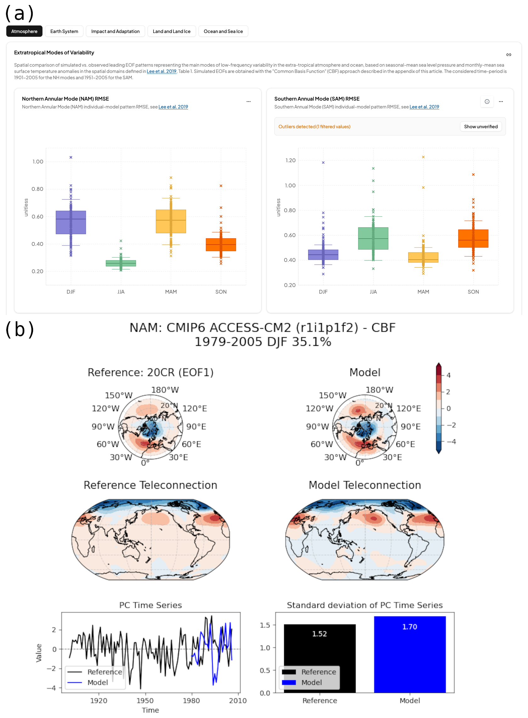
Figure 3 Evaluation metrics for the extratropical modes of variability in the atmosphere. (a) Spatial RMSE of the simulated vs. observed leading Empirical Orthogonal Function (EOF1) describing the spatial pattern of the Northern and Southern Annular Modes for a large number of historical GCM runs obtained from CMIP6. (b) Simulated vs. observed spatial pattern of the Northern Annular Mode (upper row), the mode's temporal variations in sign and amplitude as described by the principal component time series (PC) and the respective standard deviation (lower row), as well as the global SLP teleconnection pattern associated with the mode (center row); see text for more details. Figures available at https://doi.org/10.5281/zenodo.20162569 (Lee, 2026).

The results for the NAM and a specific historical simulation (the r1i1p1f2 run of the ACCESS-CM2 model) are illustrated in Fig. 3b. The simulated vs. observed EOF1 is mapped in the top row of Fig. 3b. The bottom row shows the modeled vs. observed principal component (PC) time series containing the weights to which the pattern is present at a given point in time (here: individual seasons), thus describing the sign and amplitude of the NAM over time. Also shown is a comparison of the modeled vs. observed standard deviation of the PC time series. It is here important to note that a comparison between models and observations only makes sense for climatological statistics, such as the temporal standard deviation shown here, but not for year-to-year comparisons, if the historical experiment is considered for evaluation. In the middle row, the slope obtained from regressing the grid-box scale sea-level pressure anomalies onto the PC is mapped, indicating the global teleconnection pattern associated with the NAM. A detailed description of the metric and methodology can be found in Lee et al. (2019, 2024). Results indicate that the GCMs systematically perform poorer during the winter, spring, and autumn seasons, during which the Arctic polar vortex is active, than during the summer season, when the vortex is missing. Similar results are obtained for the SH, where the polar vortex is present throughout the entire calendar year. The NAM teleconnection pattern and PC standard deviation are well reproduced by the specific model run analyzed here.

5.4.2 Land

The ability of ESMs to represent plant productivity and its seasonal variation and trend is fundamental to simulating global biogeochemical cycles, the future trajectory of atmospheric carbon dioxide, and hence, the trend in future temperatures. The REF Data Explorer offers a flexible and interactive interface for visualizing the annual cycle of gross primary production (GPP), as shown in Fig. 4a. Two models, CanESM5-1 and ACCESS-ESM1-5, were selected arbitrarily as examples to illustrate the diagnostic functionality of the REF. We can see that the CanESM5-1 model ensembles project a higher peak of global GPP than indicated by the reference data, and that peak occurs later in the season than the reference data suggests. Whereas, the ACCESS-ESM1-5 model exhibits timing resembling the reference data, the amplitude of the seasonal cycle is significantly lower than the reference data indicate.

Using diagnostics provided by the ILAMB package, the REF can evaluate model performance across pre-defined or user-defined regions. For example, as shown in Fig. 4b, the seasonal timing of the variation in GPP from the ACCESS-ESM1-5 model is approximately correct globally, although the amplitude is weak in the model. However, for the tropical region, the integrated GPP from the model is biased high, and the phase of the seasonal variation is more poorly represented. These graphical outputs help analysts and data users better understand the strengths and weaknesses of models and their implications on future projections.

Contour maps in the REF offer a visual representation of the geographic distribution of biases, as shown in Fig. 4c. Here, the month of maximum GPP in the reference data and the spatial distribution of the annual mean GPP are shown in the first column. The second column shows the same two quantities as represented by the ACCESS-ESM1-5 model, and the third column shows maps of the differences between the model and the reference data. The upper map in the third column indicates that the seasonal cycle of GPP is better represented by the model in the Northern Hemisphere than in the Southern Hemisphere, and that biases in timing of maximum GPP may lead or lag the observed timing, often by four months or more. The lower map in the third column shows that the strongest annual mean biases from the model occur in the Southern Hemisphere and that tropical biases are primarily positive and often exceed 3 g m⁻² d⁻¹.

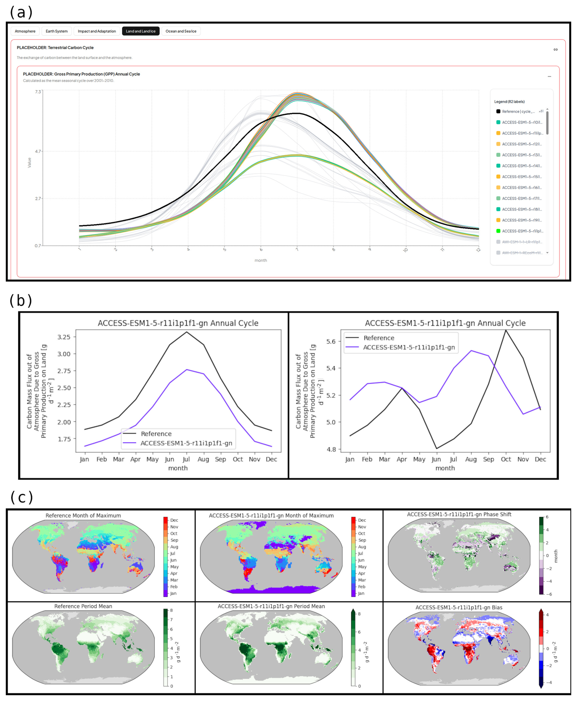
Figure 4 Shown here are example graphics produced in the REF diagnostic for gross primary production (GPP) (Diagnostic ID 2.2 in Tables 1 and ) that uses the WECANN v1.0 reference dataset (see Table A1). (a) Within the REF Data Explorer for Land and Land Ice, the gross primary production (GPP) annual cycle can be explored, and here, the CanESM5-1 model ensembles (above the black Reference line) and ACCESS-ESM1-5 model ensembles (below the black Reference line) are highlighted in color. (b) Within the REF Diagnostics for Land and Land Ice, the GPP annual cycles for global land (left) and tropical land only (right) regions for a single ensemble member from the ACCESS-ESM1-5 model are displayed. (c) ithin the REF Diagnostics for Land and Land Ice, the month of maximum GPP (i.e., the phase of the annual cycle) is shown spatially (top row) for the Reference (first column), the ACCESS-ESM1-5 model ensemble (second column), and the difference between the model ensemble and Reference (third column). Similarly, the spatial distribution of the annual integrated GPP from the ACCESS-ESM1-5 model ensemble (second column) is compared to the Reference (first column) and the resulting bias (third column) in the bottom row. Figures available at https://doi.org/10.5281/zenodo.20162790 (Hoffman, 2026).

5.4.3 Ocean

Figure 5 shows the Atlantic meridional overturning circulation (AMOC) as described in Sect. C1.2. In panel (a) we see multi-model statistics of the AMOC period mean in a box plot to summarize multi-model scalar results for comparison across the ensemble. The red colored “×” mark shows the specific model when the mouse is hovered over any of the individual model values shown as purple “×”. In panel (b), the time series of the annual area averaged time series of the ocean meridional overturning mass streamfunction is plotted for a single model and the reference data set. In panel (c) a Taylor diagram is used to compare a single model with the reference dataset.

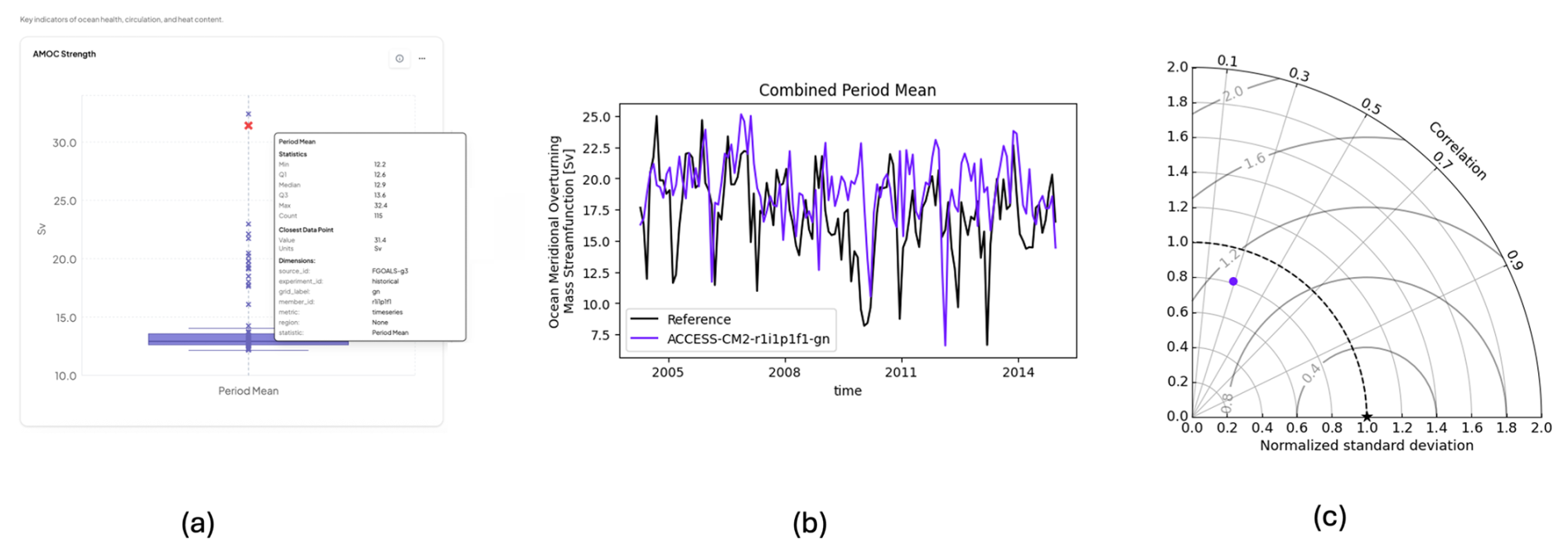
Figure 5 This is an example of the plots for the Atlantic meridional overturning circulation (AMOC) diagnostic in which the REF interactive dashboard allows users to explore results, visualize metrics, and generate plots. Figure available at https://doi.org/10.5281/zenodo.20055564 (Beadling and Swaminathan, 2026).

5.5 The Future of the REF

5.5.1 Potential New Features and Capabilities

A significant advancement for the REF will be its adaptation for daily or sub-daily GCM output in order to capture synoptic and even mesoscale phenomena such as extra-tropical blocking events (Davini and D'Andrea, 2016; Dorrington et al., 2022; Dolores-Tesillos et al., 2025; Bacer et al., 2022), storm tracks (Priestley et al., 2020), weather types (Brands, 2022; Brands et al., 2023), tropical cyclones (Roberts et al., 2020) and other phenomena. These smaller-scale phenomena are known to drive extreme events, which have direct implications for societal impacts. Model evaluation across model generations in general involve dimensionality reduction through empirical orthogonal function (EOF) analysis (Fasullo et al., 2020; Hannachi et al., 2023), k-means clustering (Hoffman et al., 2005) and/or weather regime detection (Grams et al., 2017), for which a number of efficient diagnostics tools have already been developed, e.g., Mid-latitude Evaluation System (MiLES; Davini, 2019) or GCM evaluation with Lamb Weather Types (Brands, 2025).

The REF will likely be utilized by ongoing regional WCRP initiatives such as the Coordinated Regional Downscaling Experiment (CORDEX; Sobolowski et al., 2025), the Inter-Sectoral Impact Model Intercomparison Project (ISIMIP; Warszawski et al., 2014) and the Ice Sheet Model Intercomparison Project (ISMIP; Nowicki et al., 2016), and significant potential exists to connect with other initiatives of this kind, e.g., Atmospheric River Tracking Method Intercomparison Project (ARTMIP; Rutz et al., 2019), etc. Through such collaborations, the REF can serve to foster synergies that will be mutually beneficial across research initiatives. A new collaboration effort, called the CORDEX Collection of Regional-Scale Climate Processes and Metrics for Climate Model Evaluation, will develop high-resolution diagnostics that could be integrated into the REF. As the need for higher spatial and temporal resolution grows, increasing temporal resolution is equally important for understanding extreme weather events, such as the development of tropical cyclones or heatwaves. These high-frequency variations, such as diurnal cycles or sub-daily phenomena, are key to better predicting impacts on society, and they are likely to be useful additions to the REF in the future.

Internal (or unforced) climate variability is commonly sampled by assessing the output of multiple historical (or scenario) runs of the same GCM, each initialized from different dates (branch points) of the corresponding pre-industrial control run. In these equally probable surrogates of the real climate system, the main drivers of natural variability, such as ENSO, as well as its associated teleconnections, evolve freely through time. This “initial conditions uncertainty” (Stainforth et al., 2007) produces random noise, which compared to the predictable signal exerted by external forcing agents (e.g., greenhouse gases and aerosols), is particularly large for atmospheric circulation variables such as sea-level pressure and are not directly affected by global warming (Deser et al., 2012, 2020). Consequently, GCM performance estimates for these variables are expected to be likewise affected by internal variability, especially if they are based on short time periods. However, this kind of error uncertainty has seldom been evaluated in past model performance assessments, particularly outside the atmosphere. Considering internal variability in future versions of the REF is a priority, as it will enable assignment of uncertainty ranges to model performance estimates, thereby making them more robust. This step will also improve understanding of the natural drivers of regional climates and provide better insights into how climate extremes evolve under different scenarios.

Another dimension along which the REF is expected to grow is the consideration of other components of the Earth system beyond the physical processes included in the coupled model configurations contributing to CMIP, such as atmospheric chemistry and terrestrial and marine biogeochemistry, which aim to provide a more accurate representation of the global carbon cycle (Séférian et al., 2020) and its feedback on the Earth system (Arora et al., 2020). As the community increasingly focuses on carbon emissions-driven experiments in CMIP7, the REF must be extended to quantify and reconcile carbon cycle biases (Hoffman et al., 2014) and to include the spatial and temporal evaluation of atmospheric CO₂ and CH₄ variability (Keppel-Aleks et al., 2013). This could help improve understanding of the relationships between carbon emissions and Earth system feedbacks, particularly in high-resolution models. Additionally, systematic evaluation of observed emerging signals of subsurface ocean acidification and deoxygenation, alongside warming, is desirable to benchmark transient changes (Tjiputra et al., 2023). Including these aspects will allow the REF to support a more comprehensive evaluation of oceanic changes that have substantial long-term impacts on marine ecosystems and the global carbon cycle.

The REF will be continuously exercised and updated through the CMIP7 process, and that will undoubtedly reveal opportunities for improvements. Along with such optimizations and incremental improvements, the future evolution of the REF will emerge as it is increasingly used. Many potential extensions of the REF are already envisioned, as illustrated by the above discussion. The expectation is that additional opportunities will be identified and new features will be desired as the next generation of CMIP models are scrutinized. In designing the REF, such evolution has been anticipated, and the design of the software is modular and flexible. This should facilitate community contributions to the REF. Although all the realms of ESMs are already represented by the REF, we anticipate new diagnostic packages may need to be incorporated into the REF. Packages that focus on high-frequency variability (e.g., diurnal cycle, extreme events at the sub-daily time scale) or specific phenomena (e.g., Madden-Julian Oscillation (MJO), ENSO) would be natural extensions of the current capabilities of the REF (e.g. the NOAA Model Diagnostics Task Force (MDTF) diagnostic package). Similarly, observation-based reference datasets will need to be updated as new observations are collected or new products are made available. In all of these future developments, a key aspect for the vitality of the REF will be community engagement. Community contributions and comments are welcome and necessary, as the REF is intended to be an open, community-driven project.

5.5.2 REF Governance

The MB-TT and co-sponsors of the Assessment Fast Track version of the REF agreed, based on significant community interest, that continued development of the REF should be coordinated and prioritized by an international consortium of community evaluation package developers, modelers, reference data providers, and Earth system scientists under WCRP. Such a scientific steering panel (SSP) would engage with the community to identify high priority diagnostics and reference datasets for the full set of CMIP7 simulations and other participating WCRP activities; coordinate with ESGF on quality assurance, platform upgrades, and performance enhancements; initiate and coordinate a technical development and support community; and ensure the open extensibility and portability of subsequent REF developments to support use of the evolving REF framework by modeling centers and individual researchers beyond CMIP activities. The SSP will be established to carry out these duties and to identify and propose to WCRP preferred long-term governance arrangements. An open global recruitment process will be conducted to select SSP members. Contributors to the sustainment and future engineering of the REF will likely acquire their own funding or support for collaborative maintenance and development, which will be coordinated through the REF-SSP.

6 Conclusions

The Rapid Evaluation Framework (REF) is an open source Python-based toolkit (compatible with versions ≥3.11) under active development, designed to automate and manage evaluations of Earth system model (ESM) output. The REF's primary objective is to enable near-real-time assessment of ESM output through comparison with well documented reference datasets, updating outputs dynamically as new simulation results are published. Functionally analogous to a Continuous Integration/Continuous Deployment (CI/CD) pipeline in software development, the REF streamlines continuous evaluation workflows for Earth system science. A beta version of the REF, targeted for use and testing by modeling centers and interested researchers, was released to the public on 27 May 2025.

Proposed by the MB-TT, the REF is initially deployed to support the Assessment Fast Track simulation campaign, providing diagnostics collaboratively selected by the MB-TT and the broader science community. While initially tailored for the Assessment Fast Track, the framework is intentionally agnostic to variable types and analytical metrics, ensuring adaptability for diverse Earth science applications beyond its initial scope. This extensibility underscores its potential long-term research utility. Key technical features include integration with CI/CD systems, availability on PyPI from version v0.5.0, comprehensive documentation, and community-driven development under an Apache License 2.0 open source license. Emphasizing collaboration, the REF invites contributions from researchers and developers, fostering a shared ecosystem for advancing model-data evaluation tools. The project's design prioritizes scalability and flexibility, aiming to serve as a foundational resource for real-time ESM benchmarking in both current and future research contexts. Interest in the REF across the research community is strong, and future governance of REF development will be coordinated and prioritized by a scientific steering panel that is currently being formed. A wide variety of new diagnostics are already proposed for integration in subsequent developments of the REF.

Appendix A: Reference Datasets Used by the REF

Coldewey-Egbers et al. (2025, 2015)Winker (2024); Winker et al. (2024)Solberg et al. (2023)Loeb et al. (2018)Loeb et al. (2018)Karlsson et al. (2023)Harris et al. (2020)Hersbach et al. (2020)Pastorello et al. (2020)Chen et al. (2023a, b)Martens et al. (2017); Miralles et al. (2011)Adler et al. (2017, 2003, 2018)Adler et al. (2017, 2003, 2018)Morice et al. (2021)Rayner et al. (2003)Hoffman et al. (2014)FAO and IIASA (2023)Hobeichi et al. (2019)Slivinski et al. (2019)Claverie et al. (2014, 2024)Lavergne et al. (2019)Lavergne et al. (2019)Moat et al. (2025)Copernicus Climate Data Store (2020); Sofieva et al. (2023); Coldewey-Egbers et al. (2025)Kumar et al. (2012)Wang and Mao (2021); Wang et al. (2021)Alemohammad et al. (2017)Reagan et al. (2023)

Table A1 Observationally constrained reference datasets shown here are used in the REF for comparison with model output. ^∗ Indicates reference dataset ends more than five years before the end date of the CMIP7 historical simulations.

Appendix B: Diagnostics Produced by the REF

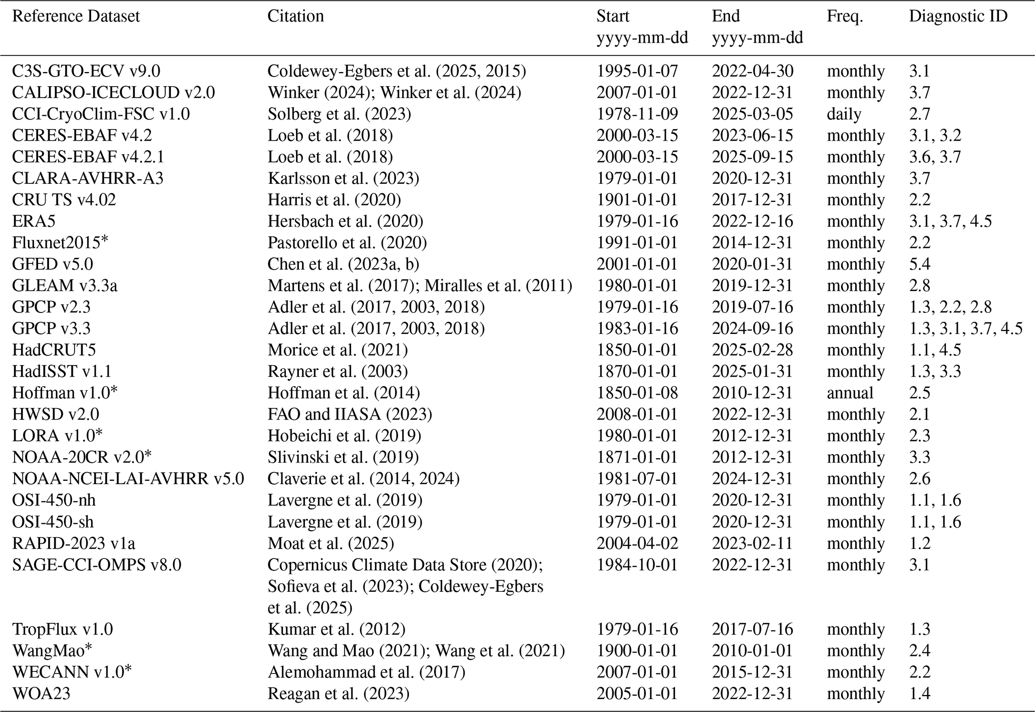
Table B1 Based on community recommendations, an initial set of diagnostics was selected, published at https://doi.org/10.5281/zenodo.20175394 (CMIP Model Benchmarking Task Team, 2026a), for incorporation into the initial version of the REF for evaluating relevant CMIP7 Assessment Fast Track simulations. Diagnostics 1.5, 5.1 and 5.2 are listed in italic style text because they were not implemented for the initial version of the REF. Diagnostic 3.4, shown in italic text, was replaced by 2.8 for the Land & Land Ice realm, and 3.5, also shown in italic text, is available as part of 1.3 and not separately. The column representing CMIP7 physical variables and branded variables does not include fixed grid information (e.g., areacella, areacello) that may be required for execution of the diagnostic.

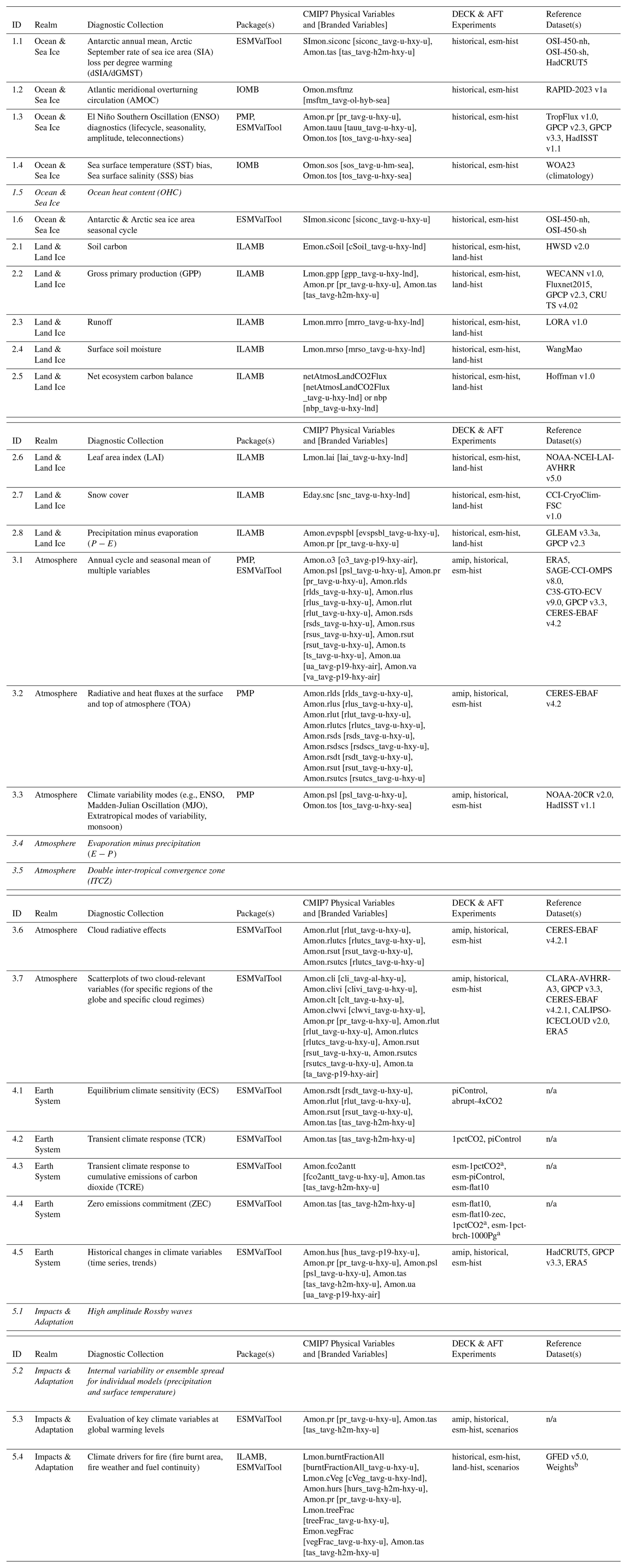
^a CMIP6 experiemnt; not available/necessary for CMIP7 Assessment Fast Track. ^b Pre-computed weights are available at https://doi.org/10.5281/zenodo.14917245 (Kelley et al., 2025). n/a – not applicable.

Appendix C: Rationale for Diagnostics Produced by the REF

This Appendix contains the list of diagnostics, v1.0 (CMIP Model Benchmarking Task Team, 2026b), originally devised by the CMIP Model Benchmarking Task Team to be implemented in the CMIP7 Assessment Fast Track Rapid Evaluation Framework (REF).

C1 Ocean & Sea Ice Realm

1.1 Antarctic annual mean, Arctic September rate of sea ice area (SIA) loss per degree warming (dSIA/dGMST)

Sea ice responds strongly to climate forcing and warming. The rapid decline in Arctic summer sea ice areal extent is a highly visible indicator of climate change. Previous sea ice benchmarking assessments have highlighted the fact that CMIP models systematically underestimate the amount of Arctic sea ice area loss per degree of global warming. Very few CMIP models are able to simulate both a plausible sea ice loss and a plausible change in global mean temperature over the satellite period. This metric evaluates the rate of sea ice loss per degree of global warming, following the approach used for sea ice benchmarking within the Sea Ice Model Intercomparison Project analysis (Notz and SIMIP Community, 2020; Roach et al., 2020). The metric is calculated by regressing the time-series of sea ice area on global mean temperature on an annual basis. The annual mean sea ice area is used for the Antarctic, while the September-mean sea ice area is used for the Arctic.

1.2 Atlantic meridional overturning circulation (AMOC)

The Atlantic Meridional Overturning Circulation (AMOC) provides a key indicator of the strength of ocean circulation, which redistributes freshwater, heat and carbon across the Atlantic Basin (Le Bras et al., 2023). A weakening of AMOC, expected to occur as a result of ocean warming, will have global climate consequences. The strength of the AMOC at 26.5° N is commonly used for evaluation of model fidelity since it can be compared with the long-term RAPID-MOCHA (Rapid Climate Change – Meridional Overturning Circulation and Heatflux Array) observational dataset (Moat et al., 2025). RAPID datasets are widely used to validate the AMOC strength in models and are available from 1 April 2005 to 11 February 2023. The AMOC at 26.5° N is calculated as the maximum of the meridional overturning streamfunction, which is provided by CMIP models as the variable “msftmz”. The AMOC is a key component of the global ocean conveyor belt and plays an important role in transporting heat poleward and ocean biogeochemical tracers from the surface into the ocean interior.

1.3 El Niño Southern Oscillation (ENSO) diagnostics (lifecycle, seasonality, amplitude, teleconnections)

The El Niño Southern Oscillation (ENSO) is the primary mode of the global interannual climate variability, mainly reflected by the variations in surface wind stress and ocean temperature in the tropical Pacific Ocean. Through teleconnections, the ENSO affects seasonal temperature and precipitation in other parts of the globe (Chen and Wallace, 2015; Vaittinada Ayar et al., 2023). The ENSO variability can be calculated from both sea surface temperature and atmospheric pressure differences between different tropical Pacific areas. The Southern Oscillation Index (SOI) uses pressure differences between the Tahiti and Darwin regions. The Oceanic Niño Index (ONI) summarizes SST anomalies in the Niño 3.4 region. Given its implications for regional climate variability, capturing the observed ENSO spatial and temporal characteristics would increase the fidelity and robustness in a model's climate projections.

1.4 Sea surface temperature (SST) bias, Sea surface salinity (SSS) bias

The SST and SSS distributions provide large scale patterns of surface ocean circulation as well as reflecting dynamical air-sea interactions and ocean-sea ice interactions in the polar regions. SST and SSS biases have a significant impact on the coupling of ESM's two majors components, the atmosphere and the ocean. Satellite data products and localized moored sensors are used to produce measurements that are incorporated into reference data to calculate SST and SSS biases in models.

1.6 Antarctic & Arctic sea ice area seasonal cycle

The sea ice area, calculated as the sum over the Northern (Arctic) and Southern (Antarctic) Hemisphere grid cell areas multiplied by the sea ice fraction within each cell, exhibits a distinct seasonal cycle. Arctic sea ice area typically has minimum values in September, while Antarctic sea ice area is lowest in February. The seasonal cycle is driven by the seasonal cycle of the insolation, sea ice processes, as well as the exchange with the atmosphere and ocean and can be seen as an overview metric for the general state of the sea ice in a model. Since sea ice has a much higher albedo than the ocean surface, sea ice area plays an important role in the surface energy and radiation budgets. In addition to the multi-year average seasonal cycle of Arctic and Antarctic sea ice area, the diagnostic also produces time series of the September (Arctic) and February (Antarctic) sea ice area.

C2 Land & Land Ice Realm

2.1 Soil carbon

Soil carbon is the organic matter and inorganic carbon in global soils. It is an important component of the global carbon cycle and affects soil moisture retention and saturation. Soils are the largest stores of carbon on Earth, and warming can impact the ability of soils to store and retain carbon, especially in the Arctic, where permanently frozen soil can release large quantities of carbon into the atmosphere if it thaws due to warming (Trumbore and Czimczik, 2008). Analyzing stored soil carbon helps track quantify the dynamics of the terrestrial carbon cycle within models and the movement of carbon through the Earth system.

2.2 Gross primary production (GPP)

Gross primary production is the process by which plants “fix” atmospheric or aqueous carbon dioxide through photosynthetic reduction into organic compounds, and it is affected by increases in atmospheric carbon dioxide (CO₂) levels and warming (Anav et al., 2015). A fraction of gross primary productivity supports plant respiration and the rest is stored as biomass in stems, leaves, roots, or other plant parts. Land use change, heat and drought stress due to anthropogenic warming, and rising atmospheric CO₂ will differentially influence gross primary production in ecosystems and alter the global carbon cycle. Thus, models must be evaluated to ensure they capture the observed responses to these changes.

2.3 Runoff

Surface water runoff plays an important role in the hydrological cycle by returning excess precipitation to the oceans and controlling how much water flows into water systems (Trenberth et al., 2007; Trenberth and Caron, 2001). Changes in atmospheric circulation and distributions of precipitation have a direct effect on changes in runoff from land. Models must be evaluated to ensure they exhibit the observed responses to precipitation and soil moisture processes that lead to runoff and transport of freshwater into rivers and oceans.

2.4 Surface soil moisture

Surface soil moisture is an important hydrological cycle variable governing interactions between the land surface and atmosphere, and with the oceans through surface water runoff. Soil moisture partitions incoming energy into latent and sensible heat fluxes and also controls how precipitation is partitioned into runoff or for evapotranspiration. It therefore is at the nexus of the carbon, energy, and water cycles and is key to understanding a broad range of processes from drought, floods to agricultural management. Models must be evaluated to ensure they exhibit observed responses in soil moisture to variation in precipitation, temperature, land use change, soil carbon content and biogeochemical cycles (Seneviratne et al., 2010).

2.5 Net ecosystem carbon balance

The net ecosystem carbon balance is a quantitative estimate of the overall terrestrial carbon uptake or loss, sometimes referred to as the land carbon sink (Keenan and Williams, 2018). The land sink represents the annual carbon uptake on land through gross primary production minus losses through ecosystem respiration, disturbance, wood and agricultural harvest, and land use change. Along with the global marine carbon sink, the global terrestrial carbon sink is important for sequestering anthropogenic carbon from the atmosphere and is influenced by climate change. Models must be evaluated to ensure they exhibit observed responses in the net ecosystem carbon balance since it directly affects the amount anthropogenic carbon retained in the atmosphere (Le Quéré et al., 2018).

2.6 Leaf area index (LAI)

Leaf area index (LAI) is a measure of the total area of leaves per unit ground area, and it is used to characterize the structure of plant canopies (Fang et al., 2019). Thus, it is an important variable to model mass and energy exchange through leaf surfaces between the biosphere and atmosphere. LAI is influenced by gross primary production and plant physiological allocation of carbon to leaves. Models must be evaluated to ensure they exhibit observed responses to seasonal and trend changes in LAI in response to variations in temperature, precipitation, soil moisture, nutrient availability, and atmospheric CO₂.

2.7 Snow cover

Globally, snow cover is a key determinant of the Earth surface albedo and is also known to affect the large-scale atmospheric circulation, particularly in the Northern Hemisphere (Barnett et al., 1989; Cohen and Entekhabi, 1999). It is also a key element of the Arctic Amplification phenomenon (Cohen et al., 2014) and directly impacts the terrestrial hydrological cycle by providing a meltwater source in mid-latitudes. On the regional scale, snow cover is a paramount climate driver in the mid-to-high latitudes of the Northern Hemisphere, where it determines the length of the winter season and associated significant changes in hydrology, soil properties, and vegetation activity. A persistent snow-cover essentially blocks interactions between the atmosphere and underlying land-surface (Bokhorst et al., 2016). Models must be evaluated to ensure they exhibit observed responses to seasonal and trend changes in precipitation, temperature, and other important driving mechanisms.

2.8 Precipitation minus evaporation (P−E)

The seasonal state of water balance on land offers insights into water availability, soil moisture, latent heat energy, and runoff. While these states and fluxes can be independently evaluated, the overall water balance on land is ultimately the input (precipitation) minus the output (evaporation) exchanges with the atmosphere. In this case, precipitation is the moisture that falls on land in any form: solid, liquid, or vapor. Here, evaporation includes evaporation of water from all surfaces, including soils, plants, impervious surfaces, and rivers and reservoirs; as well as transpiration from plants and sublimation from frozen water. Models need to be evaluated to determine, not only if the soil moisture and humidity are correct, but if they are correct because the model sufficiently captured the water balance of fluxes with the atmosphere.

C3 Atmosphere Realm

3.1 Annual cycle and seasonal mean of multiple variables

The annual cycle provides an integrative measure of skill at one of the fundamental forced time scales, yet ESMs often exhibit pathologic biases in the phase or amplitude of key quantities (e.g., Scaife et al., 2010; Hoffman et al., 2014; Miller et al., 2015). Evaluating the seasonal and annual variability in models helps to ensure that key processes are correctly represented in models.

3.2 Radiative and heat fluxes at the surface and top of atmosphere (TOA)

The radiative and heat fluxes at the surface and top of atmosphere (TOA) represent the fundamental flows of energy through the climate system. The TOA radiative budget indicates the relative disequilibrium of the climate system, and is the primary approach to quantifying the equilibrium climate sensitivity. Similarly, capturing the transient response at TOA is a basic measure of a model's ability to realistically represent the system response to forcing (Loeb et al., 2020). Fluxes at the surface quantify the energy exchange between the atmosphere and surface and are directly related to the redistribution of heat through the system and the ocean heat uptake (Mayer et al., 2024). Imbalances at the TOA in unforced experiments are a typical source of bias, inducing spurious drifts in model behavior (e.g., Mauritsen et al., 2012), inducing an erroneous interpretation of the thermodynamics of the climate system (Lucarini et al., 2017) and in particular of the relation between heat gradients and the general circulation of the coupled atmosphere-ocean system, as well as the patterns of the response of the system to an inhomogeneous forcing (Irving et al., 2019; Lembo et al., 2019). Calculations of radiative and heat fluxes at the surface and TOA are usually carried out by the radiative transfer modules in atmospheric models, and parametrization of latent and sensible heat fluxes at the surface through bulk formulas. The imbalances are obtained by combining these fluxes, whereas transports can either be implied through integration of fluxes (Trenberth and Caron, 2001), or explicitly retrieved through evaluation of the internal energy within the atmosphere (Moist Static Energy; MSE) or inside the oceans (ocean heat content; Cheng et al., 2024) and other subdomains.

3.3 Climate variability modes (e.g., NAM, NAO, NPGO, NPO, PDO, PNA, SAM)

The main modes of low-frequency variability in the atmosphere, such as the North Atlantic, Arctic and Antarctic Oscillations, the Pacific North American and Pacific South American patterns, are important drivers of climate variability on the hemispheric- to continental-scale because they determine the broad direction and strength of the atmospheric flow (Wallace and Gutzler, 1981). Since the flow determines the temperature and moisture characteristics of the air masses transported to a any specific region, these modes also explain a significant fraction of the regional-scale climate variability around the globe (Hurrell et al., 2001). Originating in the equatorial Pacific, the El Niño-Southern Oscillation (ENSO) is the most important (ocean-atmosphere) mode of climate variability and is associated with typical climate anomalies in many regions around the globe (Trenberth et al., 1998). Most of these modes are considered internal (or unforced) oscillations, meaning that their characteristics are largely robust to anthropogenic forcing (Deser et al., 2012). Due to their large scale, they are the primary diagnostics a global climate model should be able to reproduce, before one would proceed to evaluate model performance on smaller scales (Fernández-Granja et al., 2024).

3.6 Cloud radiative effects

Clouds play an important role in climate by reflecting incoming solar radiation (shortwave) and by absorbing and emitting outgoing thermal radiation (longwave). These cloud radiative effects can be quantified by calculating the differences in TOA clear-sky and all-sky radiative fluxes. The diagnostic calculates multi-year annual average shortwave and longwave TOA cloud radiative effects that are then used to create maps and zonal means of the cooling and warming effects of clouds of the models in comparison to observations.

3.7 Scatterplots of two cloud-relevant variables (for specific regions of the globe and specific cloud regimes)

Despite their pivotal role in the radiation budget and the hydrological cycle, clouds have proven notoriously challenging to simulate with global climate models. The diagnostic investigates the relationship between modeled integral cloud properties such as total cloud cover, cloud water path (sum of cloud ice and cloud liquid) and cloud ice water path and climate-relevant quantities such as long- and shortwave TOA cloud radiative effects and precipitation that can then be compared to observations. In addition, the relation between three-dimensional cloud ice water content and three-dimensional air temperature is investigated and compared to reference data.

C4 Earth System Realm

4.1 Equilibrium climate sensitivity (ECS)

ECS is defined as the change in global mean near-surface air temperature that results from an instantaneous doubling of the atmospheric CO₂ concentration after the climate system has reached its new equilibrium. To avoid having to simulate thousands of model years until the system has reached equilibrium, ECS is usually approximated with the “effective climate sensitivity” following a method by Gregory et al. (2004), which estimates ECS as the x-intercept of a linear regression of the change in global mean TOA net radiation flux against the change in global mean near-surface air temperature (see Schlund et al. (2020) for details). Even though ECS is an idealized metric, it is still relevant for policymakers and scientists since it measures the equilibrium warming response of the climate system to CO₂ forcing.

4.2 Transient climate response (TCR)

TCR is defined as the global mean near-surface air temperature change at the time of CO₂ doubling in a simulation where the atmospheric CO₂ concentration is increased by 1 % per year from the preindustrial level (Gregory et al., 2009). In practice, it is calculated by averaging the global mean near-surface air temperature change over 20-year period centered around the time of CO₂ doubling (year 70) in the 1pctCO2 increase simulation (see Meehl et al., 2020 for details). Similar to ECS, it is an idealized metric that describes the warming response of the climate system to CO₂ forcing, but unlike ECS, it does not assume radiative equilibrium of the system.

4.3 Transient climate response to cumulative emissions of carbon dioxide (TCRE)

Unlike ECS and TCR, TCRE describes the warming response of the Earth system to cumulative emissions of CO₂ instead of atmospheric CO₂ concentrations and thus takes carbon cycle feedbacks into account (Gregory et al., 2009). Following Sanderson et al. (2025), TCRE is estimated from an experiment with constant CO₂ emissions of 10 Pg C per year (“esm-flat10”) as the global mean near-surface air temperature change observed after the emission of 1000 Pg C of CO₂ (i.e., at year 100) averaged over a 20-year period (i.e., years 90–110). TCRE is one of the most important policy-relevant climate change metrics since it directly links global warming and CO₂ emissions in a linear relation, which allows a straightforward estimation of carbon budgets that remain to reach specific warming targets.

4.4 Zero Emissions Commitment (ZEC)

The Zero Emissions Commitment (ZEC) quantifies the change in global mean temperature expected to occur after net carbon dioxide (CO₂) emissions cease (MacDougall et al., 2020). ZEC is therefore important to consider when estimating the remaining carbon budget. Calculation of ZEC requires dedicated simulations with anthropogenic carbon emissions set to zero, branching off a base simulation. For CMIP7 fast track, the base simulation will be “esm-flat10”, while the dedicated simulation will be called “esm-flat10-zec” (Sanderson et al., 2025).

4.5 Historical changes in climate variables (time series, trends)

To assess the ability of climate models to look into the future, it is important to evaluate them on the changes, which have been observed in recent decades, where observations and reanalysis data provide a reference. In addition to the global mean, time series and trends of key climate variable like temperature, pressure, wind and humidity are compared regionally, using, e.g., the IPCC climate reference regions for subcontinental analysis of climate model data (Iturbide et al., 2020). A regional analysis is important to assure climatic consistency and the representation of regional features within global model data as well as climate model data with regional focus, e.g., from the Coordinated Regional climate Downscaling Experiment (CORDEX; Diez-Sierra et al., 2022; Sobolowski et al., 2025).

C5 Impacts & Adaptation Realm

5.3 Evaluation of key climate variables at global warming levels

Global warming level (GWL) exceedance years or the years at which the global mean surface temperature warms over specific values is an important marker of climate change. The exceedance years are calculated as the 21-year mean anomaly of the area averaged global mean surface temperature with respect to the pre-industrial control mean temperature as described in Swaminathan et al. (2022). Assessing global values of key climate variables such as temperature and precipitation at specific GWLs can tell us how different regions are affected by climate change and whether these changes scale linearly with increases in temperature thereby providing important information for adaptation and mitigation efforts. Evaluating climate at GWLs is also relevant for policy, for instance the UNFCCC Paris agreement's central aim is to keep warming below 2 °C and if possible below 1.5 °C.

5.4 Climate drivers for fire (fire burnt area, fire weather and fuel continuity)

Many climate models do not explicitly simulate fire processes. As a result, assessing fire risk and its impacts often relies on Fire Danger or Fire Weather Indices, which use meteorological information derived from climate models. These indices are traditionally based on daily or sub-daily data. This diagnostic constructs testable fire weather and fire fuel indices specifically designed for evaluating monthly climate model output. To achieve this, we use a Bayesian inference framework, which represents and optimizes different controls of burnt area, to generate fire weather and fire vegetation indicators from monthly observed or reanalysis meteorological and vegetation data. Assessment of meteorological and biological conditions that drive fire would aid the development of these models. Developing fire weather indices that directly target burnt area, rather than relying solely on traditional fire danger formulations, presents a more robust alternative for climate model assessment.