Implementation of a three-dimensional planetary boundary layer parameterization in a coupled modeling system and evaluation of “gray zone” simulations of a wind-wave event off the US California Coast using observations

A three-dimensional (3D) planetary boundary layer (PBL) parameterization was added to the Coupled Ocean Atmosphere Wave Sediment Transport (COAWST) model and the first coupled atmosphere/wave “gray zone” simulations were carried out using the 3D PBL parameterization. A case study of a significant wind-wave event from 4–8 November 2020 off the US west coast was examined, with a focus on the impacts of the event within an approximate 280×280 km central California coastal region covering the Bureau of Ocean Energy Management Morro Bay wind energy lease area. Simulations with both one-dimensional (1D; Yonsei University) and 3D PBL parameterizations were examined in this nest with Δx=400 m. Two-way coupling was active, with near-surface winds feeding back to the wave model and bulk wave statistics feeding back to the atmospheric model. Both simulations compared favorably with buoy observations in capturing the timing and magnitude of wind speed, temperature, dewpoint, and significant wave height, as the front associated with the maritime weather system moved southward across coastal California. However, wind speed errors over land were larger. Time series of the vertical profile of winds below z=250 m from the simulations compared favorably with observations from the US Dept. of Energy Morro Bay Doppler lidar buoy. Differences between the coupled 1D and 3D PBL simulations were minor. The most notable difference was that the simulation using the 3D PBL parameterization had approximately 10 % weaker winds at the peak of the event causing 10 % lower significant wave heights. This difference was shown to be mostly due to differences in the vertical mixing treatment between the parameterizations, in particular the nonlocal downward mixing of higher momentum air in the 1D Yonsei University parameterization in convective conditions. Overall, this work demonstrates that the 3D PBL parameterization can be used in a coupled atmosphere/wave modeling framework with similar behaviors as traditional PBL parameterizations that do not provide horizontal turbulent variances and fluxes.

1 Introduction

The US West Coast has increasingly become a focus for offshore wind turbines (Dvorak et al., 2010; Sheridan et al., 2022) due to the wind resource from the persistent, strong California summertime coastal low level jet (Zemba and Friehe, 1987; Burk and Thompson, 1996; Holt, 1996; Parish, 2000; Juliano et al., 2025). The jet maximum is typically located near the top of the marine boundary layer (z≈200–500 m), and often has winds in excess of 30 m s⁻¹ (Parish, 2000), making it ideal for harnessing the offshore wind resource. While the jet is not as persistent or strong in the winter due to the weakening of the eastern Pacific high pressure ridge, strong winds from transient weather systems and atmospheric rivers frequently affect the coast.

With limited in-situ observations over the ocean, offshore wind resource characterization requires realistic numerical model simulations to fill spatiotemporal observational gaps. Since the near-surface and boundary-layer flows where future offshore wind turbines will be deployed are influenced by waves and oceanic processes (e.g., wave-induced changes to surface roughness, and sea surface temperature changes affecting surface heat fluxes, among others), three-way coupled modeling systems are often desired for more realistic simulations. While coupled mesoscale model simulations with horizontal grid spacings of O(1 km) have generally validated well against observations (Gaudet et al., 2022), higher resolution simulations within the Terra Incognita (or “gray zone”) (Wyngaard, 2004), in which turbulence is partially resolved and partially parameterized, can further help to understand the role of O(100–1000 m) turbulent PBL structures relevant to offshore wind energy applications. In the future, coupled large eddy simulations driven by mesoscale models could explicitly resolve turbulence in the marine atmospheric boundary layer, potentially leading to more realistic simulations of the environment of offshore wind turbines. A review of challenges and opportunities of mesoscale to microscale model coupling for wind energy applications is provided by Haupt et al. (2023) and a review of the current state of the art for wind-wave coupled large eddy simulations is provided by Deskos et al. (2021).

The conventional approach to PBL parameterization with grid spacings of O(1 km) or greater is to parameterize the sub-grid-scale vertical mixing only; the horizontal Reynolds stresses and flux divergence terms are neglected and a grid-scale deformation-based approach to horizontal mixing is applied (Smagorinsky, 1963). However, as the grid spacing decreases to within the “gray zone” [O(100–1000 m)], this assumption is no longer valid because the horizontal Reynolds stress and flux divergence terms can be of similar magnitude as the vertical terms (Kosović et al., 2020). To address this deficiency, a 3D PBL parameterization has been developed (Kosović et al., 2020; Juliano et al., 2022). In the 3D PBL parameterization, the horizontal Reynolds stresses and fluxes are parameterized using the Mellor-Yamada closure model, and grid-scale horizontal mixing is calculated through their respective divergences in the Reynolds Averaged Navier Stokes equations. To date the 3D PBL parameterization has been mostly evaluated in idealized cases (Juliano et al., 2022). Prior to this work, the 3D PBL parameterization had not yet been coupled to wave and ocean models, nor has the 3D PBL parameterization been significantly evaluated for more complex flows over coastal regions with steep, complex terrain. More complex real cases will help to better assess the performance of the 3D PBL parameterization.

The atmospheric momentum and surface gravity wave field over the ocean are intimately coupled, leading to momentum and heat exchanges (Sullivan and McWilliams, 2010; Edson et al., 2013; Patton et al., 2019). Uncoupled atmospheric simulations that do not account for dynamic wave fields typically use sea surface roughness parameterizations such as Fairall et al. (2003) and Charnock (1955), which account for increased roughness as the surface stress increases from higher winds. Spectral models such as Wave Watch III (Tolman, 1997; Pringle and Kotamarthi, 2021) solve for the wavenumber-direction spectra of resolved waves, leading to dynamic changes in roughness due to the varying wave field, e.g. changes in the height and steepness of the waves (Taylor and Yelland, 2001), wave age (Drennan et al., 2003), and wave-wind misalignment. Due to the differences in the near-surface wind field between simulations using 1D and 3D PBL parameterizations, differences in wind-driven waves might arise leading to differences in momentum exchanges between the atmosphere and ocean. An understanding of these differences would be of interest for better characterization of the offshore wind resource. Moreover, evaluation of both near-surface wind and wave forecasts between simulations using 1D and 3D PBL parameterizations would provide insight into which parameterization is more consistent with observations.

The purpose of this paper is to describe the implementation of a 3D PBL parameterization in a coupled wave/ocean/atmosphere modeling system and to evaluate “gray zone” simulations with both 3D and 1D PBL parameterizations using observations for a significant wind-wave event that occurred off the US west coast from 4–8 November 2020. The primary way that 1D and 3D PBL parameterization simulations will differ on the time scale of days is through momentum exchanges associated with the two-way feedback of near-surface wind speeds and waves; sea surface temperature (and associated heat flux) changes from ocean coupling and current-wave interactions are of lesser importance. Therefore, our first goal is to perform coupled simulations with atmosphere/wave coupling only. Through this work, we will demonstrate that a coupled simulation using the 3D PBL parameterization behaves qualitatively similar to a coupled simulation using a 1D PBL parameterization. Some key quantitative differences and areas where the 3D PBL parameterization improves upon 1D PBL parameterizations will be identified.

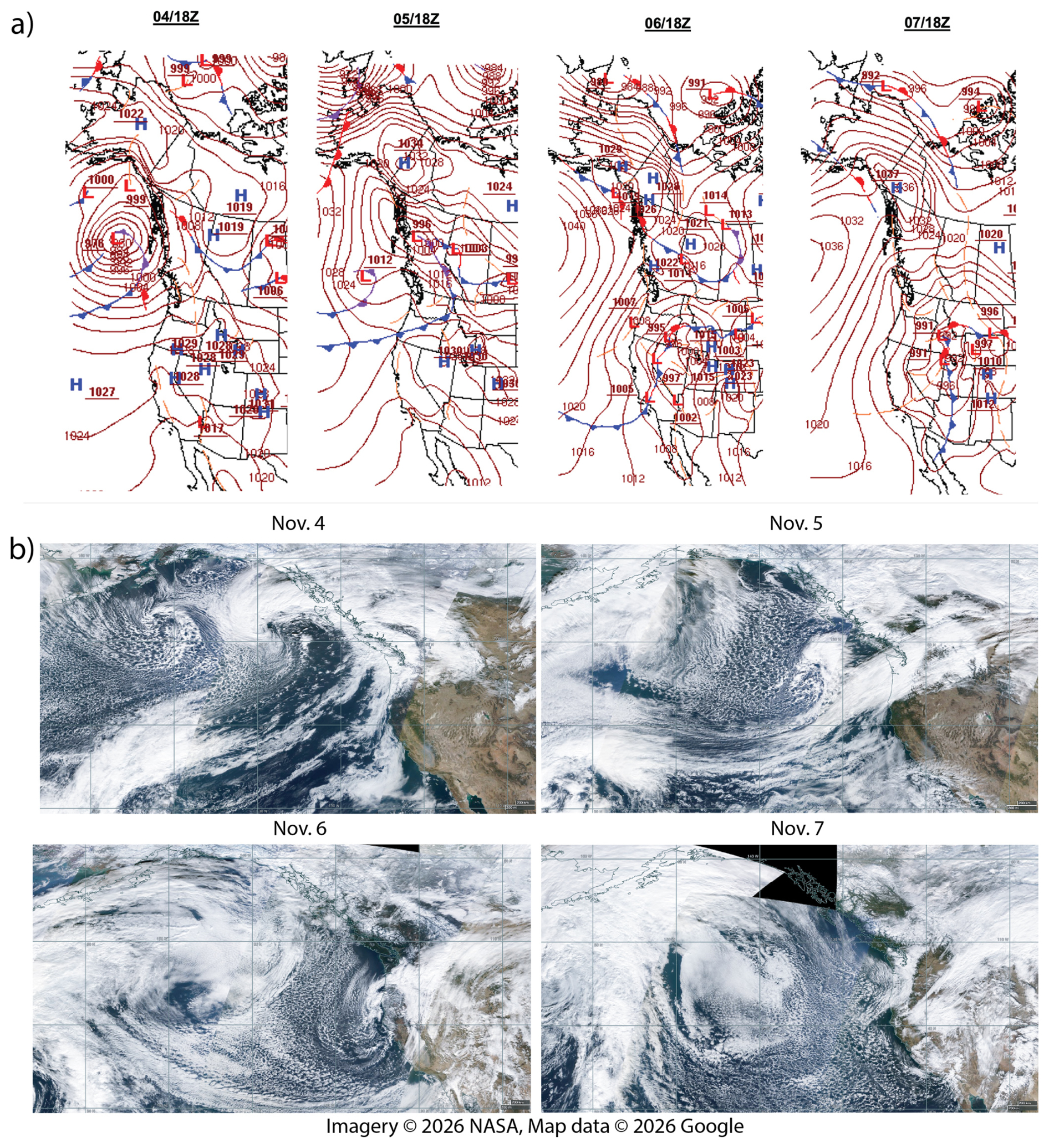
Figure 1 (a) National Oceanic and Atmospheric Administration (NOAA) Weather Prediction Center archived surface analysis maps for the case study of 4–8 November 2020 and (b) National Aeronautical and Space Administration (NASA) Moderate Imaging Spectrometer (MODIS) true color daily composite images. Imagery © 2026 NASA, Map data © 2026 Google.

2 Data and methods

2.1 Case study

We select a case study of a significant weather event that occurred off the US West Coast during 4–8 November 2020. A strong low pressure system [mean sea level pressure (MSLP) of 976 hPa] initially impacted the western Canadian coast on 4 November (Fig. 1a). The low pressure weakened while the cold front moved southward on 5 November. By 6 November, a strong maritime high pressure system with a MSLP of 1040 hPa built in behind the cold front while the cold front moved farther south over central California. Lower surface pressures were analyzed near the coast. Finally, by 7 November the cold front had moved farther south and the high pressure ridge covered a larger oceanic region behind the front. The NASA MODIS composites initially showed some high cirrus and low stratus clouds near the California coast ahead of the front (Fig. 1b, 4 and 5 November). After the front passed on 6 November, a convective cumulus and stratocumulus cloud field exists over the ocean as the colder air surged south (Fig. 1b, 6 and 7 November).

2.2 Coupled wave-atmosphere model simulations

The Coupled Ocean Atmosphere Wave Sediment Transport (COAWST) model (Warner et al., 2010) was used to simulate this event. We used two-way coupling between the Weather Research and Forecasting (WRF) Model (Skamarock et al., 2019) and Wavewatch III (WW3) (Tolman, 1997) in the COAWST modeling system, accomplished through the Model Coupling Toolkit (Larson et al., 2005). Every 30 min, the WRF model 10 m zonal and meridional velocities are passed to WW3 and the wave characteristics (significant wave height, wave period, and wavelength) are passed to the WRF model surface-layer parameterization. In the surface-layer parameterization, the time-varying surface roughness length is calculated from the wave parameters (Taylor and Yelland, 2001), with a specified Charnock parameter relation. The momentum stress vector accounts for the directional discrepancy between wind vectors and wave fields. More details on the wave-atmosphere coupling in the COAWST model can be found in Gaudet et al. (2024), Warner et al. (2010), and Pringle and Kotamarthi (2021). Lateral and initial boundary conditions were from the European Center for Medium Range Weather Forecasting Reanalysis version 5 (ERA5; Hersbach et al., 2020) at 3-hourly frequency. The numerical simulations were initialized at 00:00 UTC 4 November 2020 and integrated to 00:00 UTC 8 November 2020 (96 h). Two domains were used: an outer domain (d01) with Δx=2 km (638×755 points) and inner domain with Δx=400 m (691×776 points) [factor of 5 reduction in grid spacing]. One-way nesting was used; the inner domain did not feed back to the outer domain in the inner domain imprint region. On both WRF domains, ninety vertical levels were used. The model time step on the WRF model d01 was 10 s and the time step on d02 was 2 s. The model top was 50 hPa. To help constrain the large-scale evolution with the analysis, large-scale Newtonian relaxation to the ERA5 reanalysis was applied on the WRF model d01 with nudging coefficients of $\mathrm{3}\times {\mathrm{10}}^{-\mathrm{4}}$ s⁻¹ for winds and potential temperature ($\mathrm{1}/e$ damping time of 0.93 h), and $\mathrm{3}\times {\mathrm{10}}^{-\mathrm{5}}$ s⁻¹ for water vapor mixing ratio ($\mathrm{1}/e$ damping time of 9.3 h). Newtonian relaxation was not applied within the boundary layer.

On the WRF model d01, the Yonsei University (YSU) (Hong et al., 2006) PBL parameterization was used. On the WRF model d02, two WRF model simulations were executed using different PBL parameterizations: YSU and the 3D PBL parameterization (Kosović et al., 2020; Juliano et al., 2022) with the PBL approximation. Aside from the PBL parameterization, both d02 WRF model simulations used common physical parameterizations: aerosol-aware Thompson-Eidhammer microphysical parameterization (Thompson and Eidhammer, 2014), Rapid Radiative Transfer Model Global (RRTMG) shortwave and longwave radiation parameterization (Iacono et al., 2008), the unified Noah land surface model (Tewari et al., 2004), and the revised MM5 surface layer parameterization (Jiménez et al., 2012). The single WW3 domain was approximately the same size as the WRF model d01 and had a grid spacing of Δx=2 km. While inclusion of ocean coupling (and three-way feedback) would be more realistic, our primary goal was to understand differences in 1D and 3D PBL parameterizations with atmosphere/wave coupling only without the added complexity of oceanic processes. In future work, we will include ocean coupling to understand the impact of sea surface temperature changes and ocean currents.

2.3 Implementation of the 3D PBL parameterization

Since the focus was analysis of the different PBL parameterizations on the innermost domain in the “gray zone” with Δx=400 m, more details of the parameterizations are given here to understand their behaviors. In the first-order-closure YSU PBL parameterization, SGS vertical mixing is treated through a prescribed eddy-viscosity profile dependent on the surface fluxes (a so-called K-profile parameterization). Nonlocal vertical mixing is accomplished through a gradient correction term. The 3D PBL parameterization is based on the local, 1.5-order prognostic turbulence kinetic energy (TKE) closure Mellor-Yamada SGS model (Mellor, 1973; Mellor and Yamada, 1974, 1982). The 3D PBL parameterization calculates the Reynolds stresses and fluxes in the Mellor-Yamada level 2.5 model, and both horizontal and vertical mixing is treated through the grid-scale turbulent stress and flux divergences. Thus it does not use the 2D Smagorinsky (Smagorinsky, 1963) deformation-based grid-scale mixing in the horizontal directions like 1D PBL parameterizations such as the YSU parameterization. There are two variants of the 3D PBL parameterization (Juliano et al., 2022): the full application and an approximation. In the 3D PBL approximation, horizontal derivatives of mean quantities are neglected in the Mellor-Yamada model. The 3D PBL parameterization can be applied in simulations with horizontal grid spacings of O(100–1000 m) (the “gray zone”) where 3D effects are important since the most energetic turbulent eddies are neither fully parameterized nor fully resolved. Implementation of the 3D PBL parameterization in the COAWST modeling system involved adding and modifying several WRF model dynamics and physics FORTRAN codes and compiling and linking with the Intel Math Kernel Library (MKL), needed for linear algebra problems described in Eqs. (19) and (22) of Juliano et al. (2022). Due to computational expediency, we used the 3D PBL approximation for the simulation (henceforth labeled “3D PBL”).

2.4 Observations

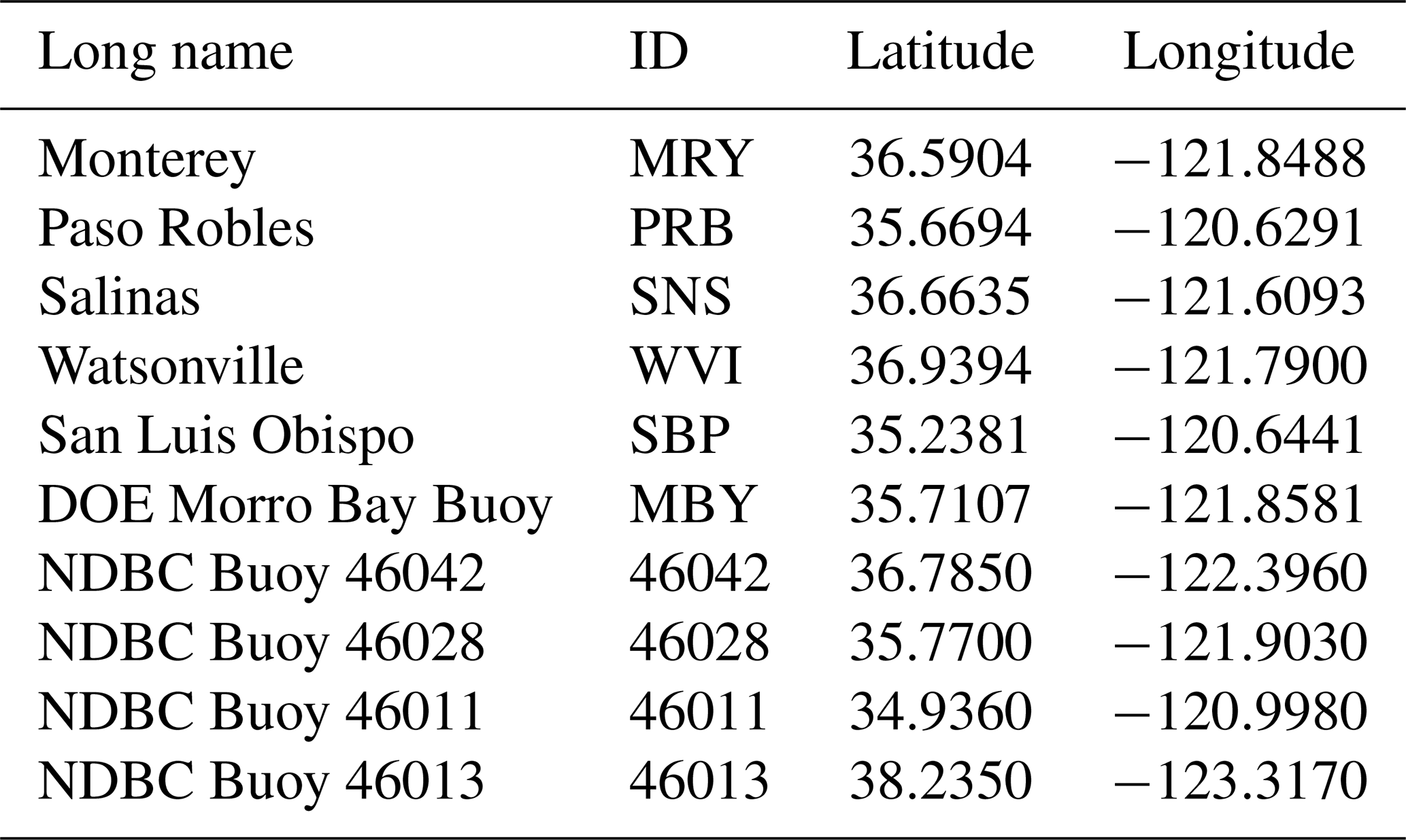
The observations used in the evaluation are listed in Table 1 and shown geographically in Fig. 2. They consist of surface meteorological stations and buoys in the area of interest, as well the vertically profiling US Dept. of Energy Morro Bay lidar profiling buoy (MBY). One buoy outside the WRF model d02 (NDBC buoy 46013, located at [38.235° N, 123.317° W], approximately 80 km north of the WRF model d02 northern lateral boundary, is also used to evaluate the WRF model d01 inflow to the WRF model d02.

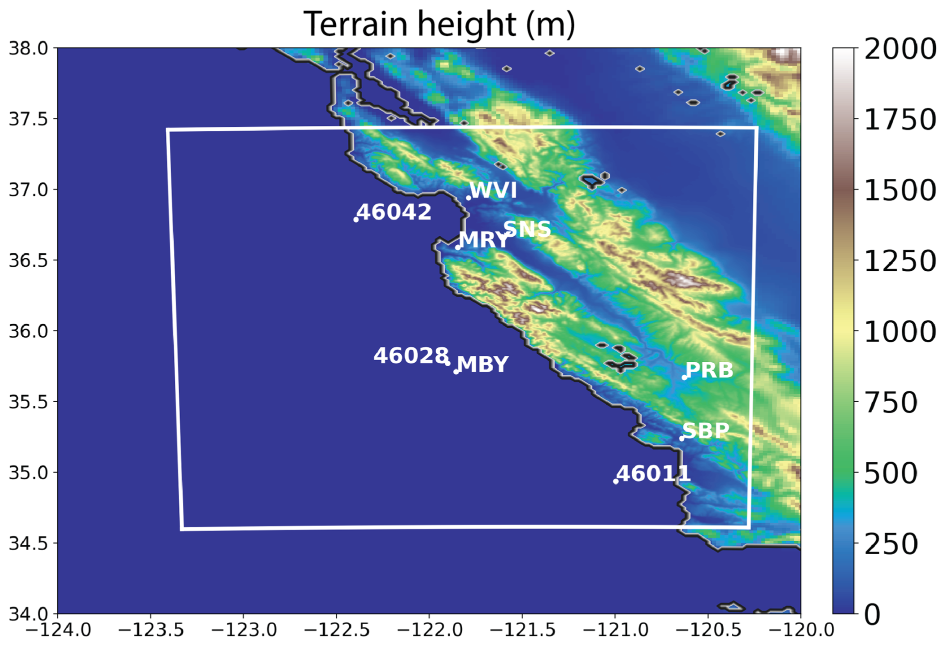
Figure 2 Zoomed in view of the WRF model terrain height (m) near the WRF model d02 with buoys and surface meteorological stations used in the evaluation in white. The WRF model d02 is outlined in white and terrain height is shown at each domain's horizontal resolution. In this figure and subsequent two-dimensional plan-view figures over geographic regions, the y axis is latitude in degrees north and the x axis is longitude in degrees east.

Table 1 Surface meteorological stations and National Data Buoy Center (NDBC) and Dept. of Energy (DOE) buoys used in the evaluation.

3 Results

3.1 Large-scale evolution

The large-scale evolution of this event on the WRF model d01 is shown in Fig. 3. The WRF model 10 m winds on both d01 and d02 fed back to WW3 in the WW3 domain (Δx=2 km; similar size to the WRF model d01), and the WW3 model fed back to the WRF model d01 and d02 with wind-wave-induced roughness changes. At 12:00 UTC 5 November, 10 m wind speeds were approximately 6–10 m s⁻¹ within the WRF model d02. Significant wave heights were approximately 2–2.5 m. As the simulated front passed around 12:00 UTC 6 November, wind speeds increased to 10–14 m s⁻¹ and significant wave heights increased to 3.5–4.5 m. By 12:00 UTC 7 November, wind speeds increased to 14–18 m s⁻¹ west of the WRF model d02 west lateral boundary, and significant wave heights increased further to peaks of 6–6.5 m. As the cold front moved south, 2 m air temperatures decreased approximately 3 °C from 12:00 UTC 6 November to 12:00 UTC 7 November (not shown). Overall there is a significant spatial correlation between the wind and wave fields, indicating this event is largely a wind-wave instead of a swell-wave event. For the remainder of the analysis, the focus will be on the WRF model d02 and differences between 1D and 3D PBL parameterizations.

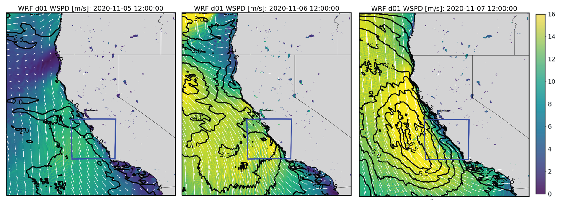
Figure 3 Large-scale evolution of the WRF model d01 10 m winds (filled contours) and WW3 significant wave heights (black contour lines). The WRF model d02 is outlined in blue. Vectors are shown in white every 25 model grid points.

3.2 Near-surface and hub-height analysis

Inspection of 24 h time means before and after the frontal passage on the WRF model d02 at z=10 m and z=206.5 m, the latter of which is one of the WRF model vertical levels that is within the typical range of hub heights for offshore wind turbines (z=75–225 m) (Sheridan et al., 2022), show persistent regions where consistent differences between the COAWST YSU and 3D PBL simulations existed (Fig. 4). Prior to the frontal passage, near-surface winds in the COAWST YSU simulation were less westerly and stronger over the ocean than the COAWST 3D PBL simulation (Fig. 4a), while at z=206.5 m the COAWST YSU simulation had northwesterly winds that were weaker. Interestingly, there was a narrow central coastal band where the COAWST YSU simulation had 1–2 m s⁻¹ stronger onshore winds at 10 m a.g.l. (above ground level). Time-mean winds before the frontal passage over the ocean were approximately 10–14 m s⁻¹ in both simulations. The simulated front passed at approximately 12:00 UTC 6 November, and after the passage, time-mean wind speeds were much larger in both simulations, particularly in the southern portion of the WRF model d02 (approximately 14–18 m s⁻¹). The COAWST YSU simulation near-surface winds were stronger over the ocean (by approximately 0.5–1.5 m s⁻¹) (Fig. 4b). At z=206.5 m, the COAWST YSU simulation winds were also stronger over the ocean, but by only approximately 0.5 m s⁻¹ on average. Significant wave heights were approximately 1–3 m prior to the frontal passage and 4–6 m afterwards (Fig. 3).

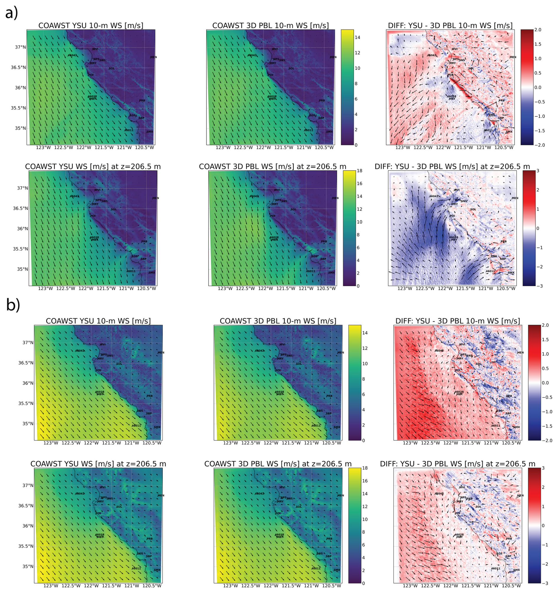
Figure 4 Time-mean wind speeds at z=10 m and z=206.5 m above sea or ground level. (a) 12:00 UTC 5 November to 12:00 UTC 6 November, and (b) 12:00 UTC 6 November to 12:00 UTC 7 November. In each panel the left plot is the YSU simulation, the middle plot is the 3D PBL simulation, and the right plot is the difference field: YSU minus 3D PBL. In the difference plots, filled contours show differences in wind speed magnitude while vectors are the vector difference.

Instantaneous difference fields of the 10 m winds and significant wave heights on the WRF model d02 every 12 h are shown in Fig. 5. Prior to 10:00 UTC 6 November, the COAWST YSU simulation had 10 m winds that were stronger over the western part of the domain, and weaker near the coast. This simulation had significant wave heights that were approximately 0.1 m larger in the western portion of the domain and 0.1 m smaller near the coast. When the significant wave heights increased after the simulated frontal passage, COAWST 3D PBL simulation winds on average were weaker over the ocean, causing significant wave heights that were approximately 0.2–0.3 m lower than the COAWST YSU simulation.

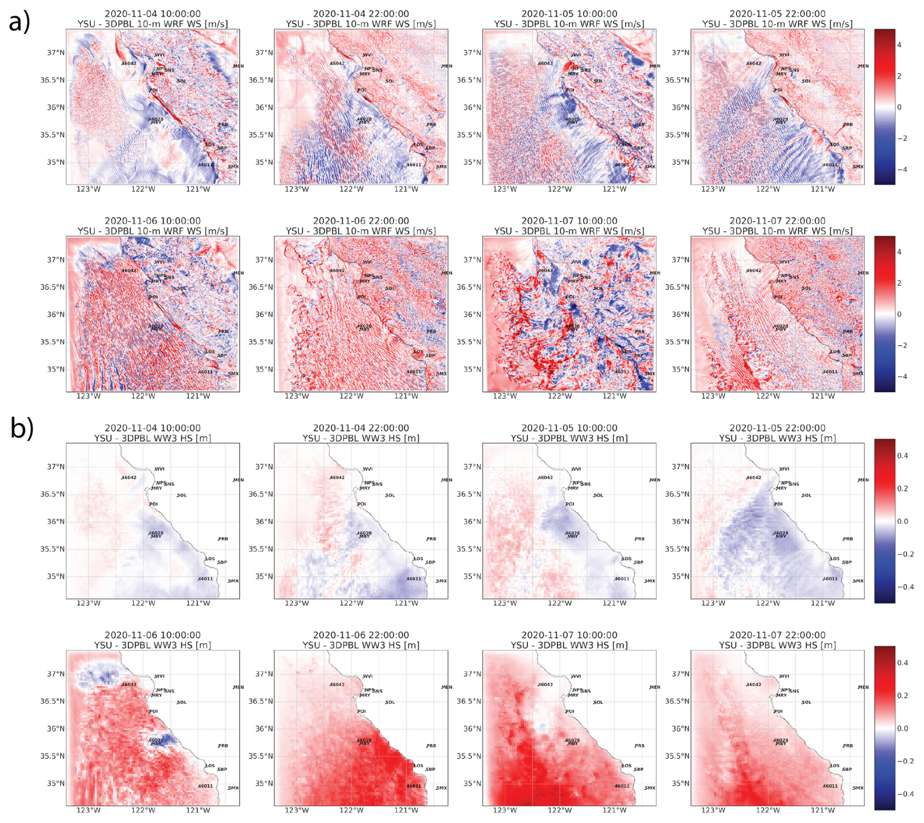
Figure 5 Instantaneous difference fields of (a) 10 m wind speeds (m s⁻¹) and (b) significant wave heights (m) every 12 h beginning at 10:00 UTC 4 November 2020. Difference is defined as the YSU simulation minus the 3D PBL simulation.

3.3 Time-mean vertical cross sections

The time-mean longitude-height vertical cross sections through the center latitude of the WRF model d02 (Fig. 6) show that prior to the frontal passage the winds were strongest near the top of the boundary layer (sloping from z≈400 m to z≈250 m, moving from west to east, marked by the sharp potential temperature inversion) with weaker winds aloft. The COAWST YSU simulation had weaker winds (by approximately 1 m s⁻¹) within the boundary layer than the COAWST 3D PBL simulation on average (except for right near the surface, as seen in Fig. 4a). After the simulated frontal passage, the boundary layer deepened and momentum became more vertically well mixed. During this period, the COAWST YSU simulation had stronger winds below z≈500 m, and weaker winds above. This is possibly due to the nonlocal mixing in the YSU PBL parameterization during the more convective conditions, vertically mixing higher momentum air downward. The COAWST YSU simulation had greater water vapor content above the boundary layer than the COAWST 3D PBL simulation (Fig. 6c). After the frontal passage, the boundary layer deepened and water vapor became well mixed vertically (Fig. 6d). During this period, over the ocean, the COAWST YSU simulation had slightly less water vapor content below z≈500 m and greater content above. Vertical cross sections of cloud water content indicated a stratus cloud field below the inversion prior to the frontal passage in both simulations (Fig. 6e). The COAWST YSU simulation had greater cloud water content near the surface near the coast than the COAWST 3D PBL simulation. After the frontal passage, with cooler air advecting over the ocean, cumulus cloud fields developed in both simulations with bases above z≈1000 m (Fig. 6f). Differences arose due to phase offsets of individual cumulus cells.

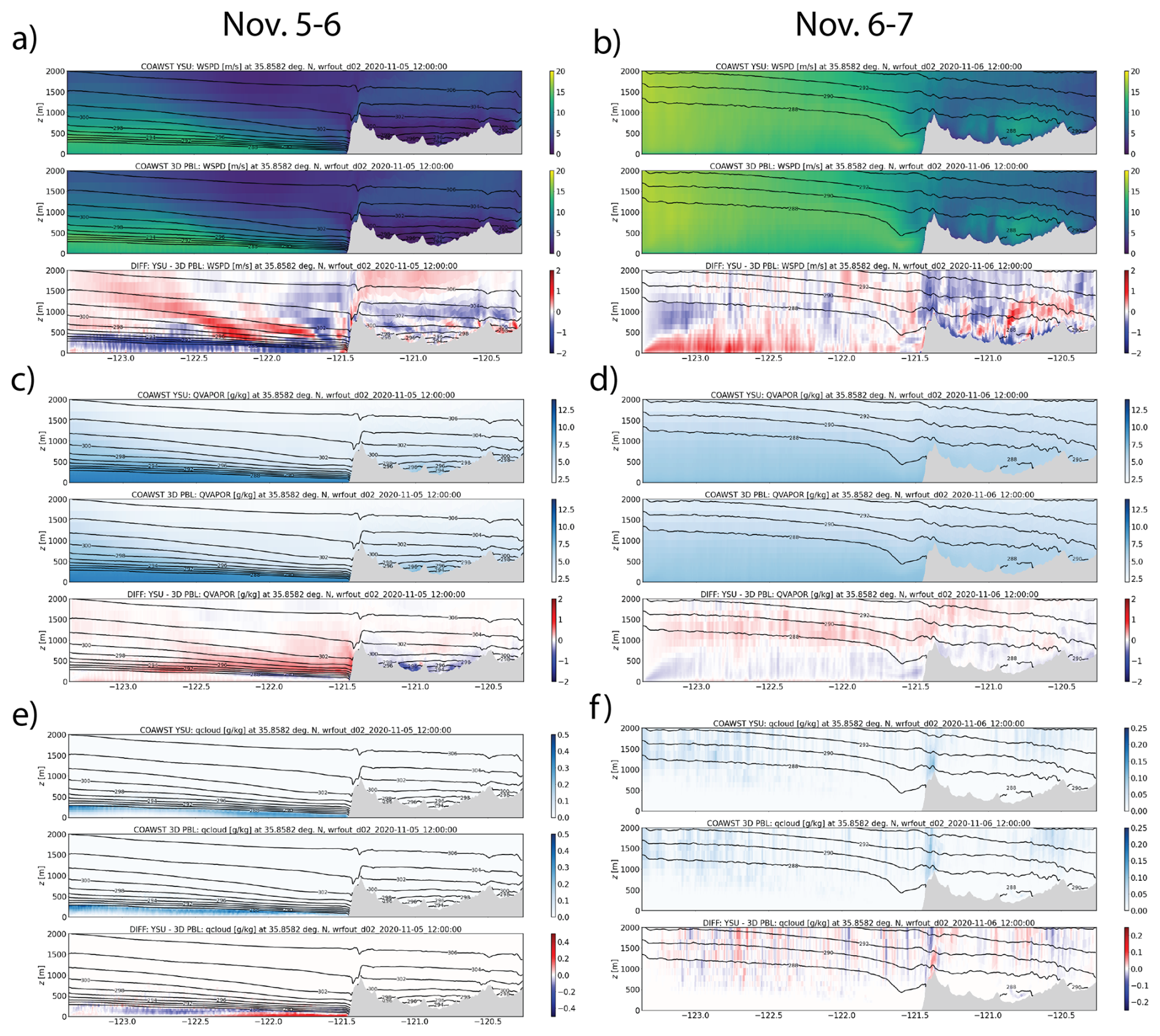
Figure 6 Longitude-height vertical cross sections of time-mean wind speed (m s⁻¹), mixing ratio (q_v; g kg⁻¹), and cloud water content (q_c; g kg⁻¹) from 12:00 UTC 5 November to 12:00 UTC 6 November (a, c, e) and 12:00 UTC 6 November to 12:00 UTC 7 November (b, d, f). (a, b) Wind speed, (c, d) q_v and (e, f) q_c. In each panel the top plot is the COAWST YSU simulation, the middle plot is the COAWST 3D PBL simulation, and the bottom plot is the difference field: YSU minus 3D PBL. In all plots, isolines of potential temperature are shown in black.

3.4 Time series analysis at near-surface buoys and stations

Time series comparisons of wind speed and direction between the COAWST model d02 and d01 simulations and NDBC buoy observations are shown in Fig. 7. Since NBDC buoy 46013 was north of the WRF model d02, only the WRF model d01 time series is shown there. Overall, all simulations capture the wind speed and direction at the buoys well: in particular, the timing and magnitude of the wind speed increase between 12:00–18:00 UTC 6 November and the change in wind direction from northwesterly to more westerly near 06:00 UTC 7 November. Examining the overall biases and errors¹, no simulation was significantly better than another.

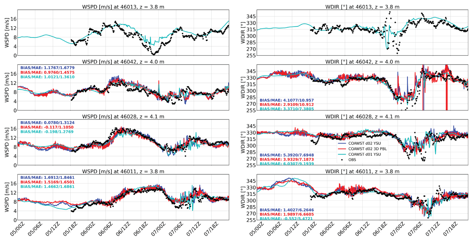
Figure 7 Model time series (COAWST d02 YSU in blue; COAWST d02 3D PBL in red; and COAWST YSU d01 in cyan) of wind speed and direction at NDBC buoys 46911, 46013, 46028, and 46042, along with buoys observations (solid black circles). Biases and mean absolute errors (MAE) are shown on the plots with multiple curves after 24 h spin-up period. The WRF model d01 time series interval is 10 s, the WRF model d02 time series interval is 2 s, and the observations are 1 min averages. Statistical performance measures are shown on plots with observations and COAWST d02 model time series. The 10 m wind speeds in the simulations are extrapolated to the buoy height using a log-layer assumption with an ocean surface roughness length of z₀=0.0002 m.

Time series of simulated temperature and dewpoint (calculated using the standard formula from mixing ratio and pressure) in comparison to buoy observations are shown in Fig. 8. North of the WRF model d02, at NDBC buoy 46013, the WRF model d01 simulation had temperatures that were approximately 1–2 °C warmer than the observations. The simulated dewpoints were more consistent with the observations, although errors were larger during the decrease between 06:00–18:00 UTC 6 November. At buoy 46042 toward the northern part of d02, the COAWST YSU and 3D PBL simulations were also slightly warmer than the observations. The decrease in dewpoint of 4 °C between 06:00–18:00 UTC 6 November was captured well by all simulations, while between 12:00–18:00 UTC 7 November, all simulations were too dry. All simulations matched the observed temperatures well at buoy 46028 after 06:00 UTC 6 November. Interestingly, the COAWST 3D PBL simulation matched the observations best after 12:00 UTC 7 November, while the COAWST YSU d01 and d02 simulations were approximately 1 °C too warm. Similar to buoy 46042, the dewpoint drop is captured well by all simulations at buoy 46028 (although the minimum simulated dewpoints were slightly lower than the observations at 18:00 UTC 6 November). At buoy 46011, unfortunately there were no observations in which to verify the model simulations. Examining the overall biases and errors, no simulation was significantly better than another.

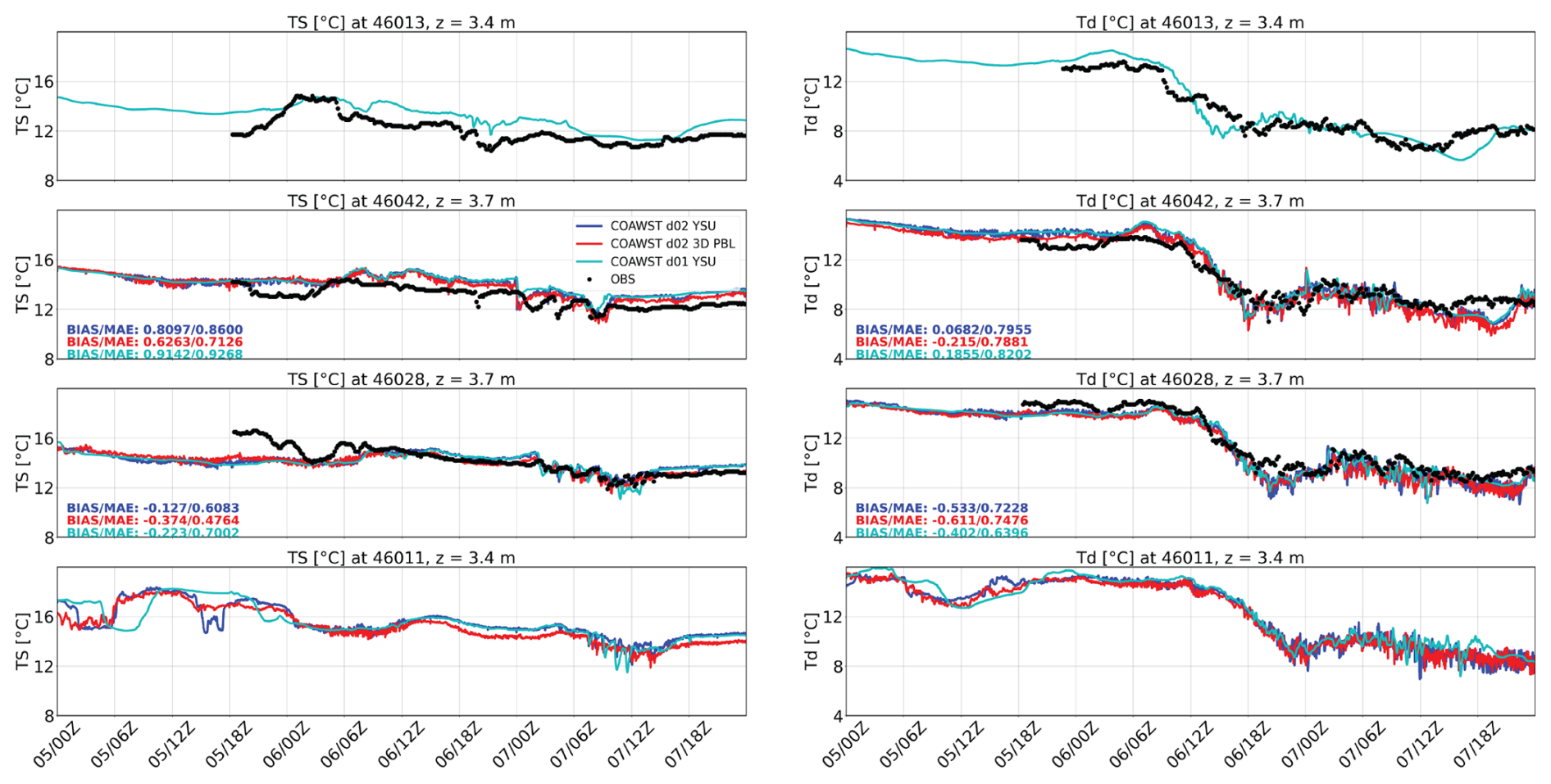
Figure 8 Model time series (red, blue, and cyan curves) of 2 m temperature and dewpoint at NDBC buoys 46911, 46013, 46028, and 46042, along with buoy observations (solid black circles). Biases and mean absolute errors (MAE) are shown on the plots with multiple curves after 24 h spin-up period. The WRF model d01 time series interval is 10 s, the WRF model d02 time series interval is 2 s, and the observations are 1 min averages. Statistical performance measures are shown on plots with observations and COAWST d02 model time series.

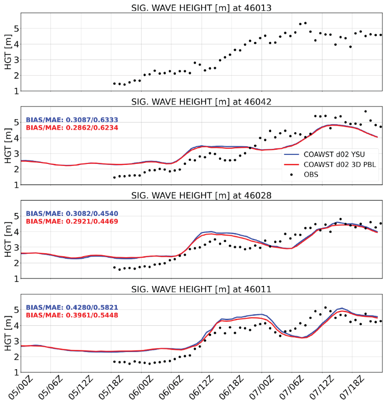
Figure 9 Model time series (COAWST d02 YSU in blue; COAWST d02 3D PBL in red) of significant wave height at NDBC buoys 46911, 46013, 46028, and 46042, along with buoys observations (solid black circles). Biases and mean absolute errors (MAE) are shown on the plots with multiple curves after 24 h spin-up period. The WW3 model time series and observations are at hourly frequency. Statistical performance measures are shown on plots with observations and COAWST d02 model time series.

Figure 9 shows the evaluation of significant wave heights at the same buoys. At all buoys, the COAWST d02 YSU and 3D PBL simulations qualitatively captured the increase from 1–2 m near 00:00 UTC 6 November to 4–6 m near 12:00 UTC 7 November due to the near-surface wind increases. At buoy 46042, very minor differences existed between the simulations, while at buoys 46028 and 46011, the differences were slightly larger. At buoy 46042, both simulations had wave heights that were approximately 0.5 m too high between 18:00 UTC 5 November and 18:00 UTC 6 November, and wave heights approximately 0.5 m too low afterwards. At buoys 46028 and 46011, the COAWST 3D PBL simulation predicted slightly lower wave heights than the COAWST YSU simulation (by approximately 0.2 m) between 12:00 UTC 6 November and 06:00 UTC 7 November, and were more consistent with the observations. At buoy 46011, the simulations captured the general increasing trend and produced the two peaks evident in the observations, although a 6 h phase lag was apparent in the simulated second maximum relative to observations.

At the over-land stations farther north (MRY, SNS, and WVI), the peak simulated wind speeds were lower than observed (Fig. 10). In particular, the observed maxima between 06:00–15:00 UTC 6 November were underpredicted at SNS and MRY. However, the simulations cannot be evaluated beyond 15:00 UTC 6 November due to missing observational data. The COAWST d02 simulations with Δx=400 m had higher wind speeds than the COAWST d01 simulation with Δx=2 km near the time of peak winds. At SPB, the model simulations generally overpredicted the wind speeds. At PRB, near 12:00 UTC 6 November, both COAWST d02 simulations overpredicted the wind speeds while the COAWST d01 simulation matched the observations better. Unfortunately, observations dropped out at all over-land stations during the peak of the wind event near 18:00 UTC 6 November to 00:00 UTC 7 November, and afterwards.

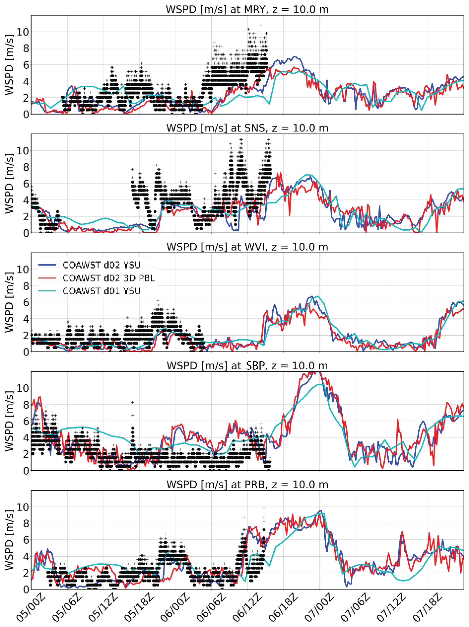
Figure 10 Model time series (COAWST d02 YSU in blue; COAWST d02 3D PBL in red; and COAWST YSU d01 in cyan) of wind speed (WSPD) at the meteorological stations over land. 1 min mean observations are in solid black circles and 5 s gusts are in plus signs. The WRF model d01 time series interval is 10 s and the WRF model d02 time series interval is 2 s.

3.5 Time series analysis at the Morro Bay lidar buoy

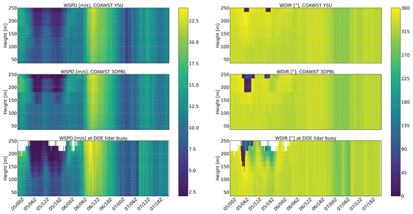
The COAWST simulated wind speed and direction at the Morro Bay lidar buoy (MBY) compared favorably in both the timing and magnitude (Fig. 11). Prior to approximately 06:00 UTC 6 November, there was a stronger vertical gradient in both the simulations and observations, with weaker winds aloft and stronger winds near the surface. As the front moved through the domain near 12:00 UTC 6 November, wind speeds became more well mixed vertically. The timing of the wind maximum between 06:00–12:00 UTC 6 November was well captured by both COAWST d02 simulations. The second wind maximum near 09:00 UTC 7 November was also captured in both simulations, but more diffuse in time in comparison to the lidar observations. Wind directions were generally northwesterly near the surface and turning more northerly aloft before 12:00 UTC 6 November. Wind directions were more uniform vertically afterwards, and exhibited northwesterly flow. The turning of the flow to more westerly between 00:00–06:00 UTC 7 November was captured well by both COAWST simulations.

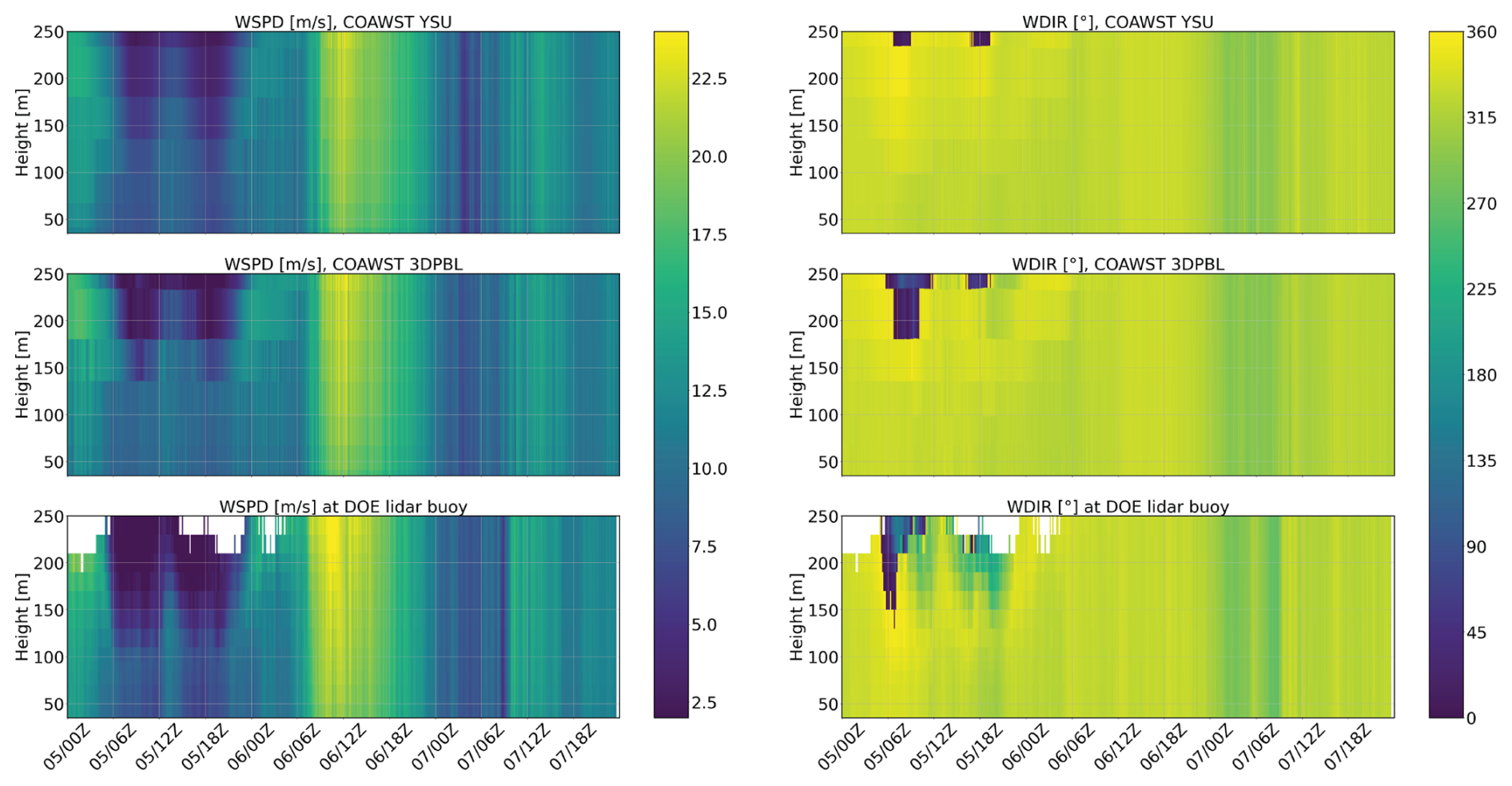
Figure 11 Time-height plot of simulated wind speed and direction from both COAWST YSU and 3D PBL simulations at the DOE Morro Bay lidar Buoy, along with lidar buoy observations. In the bottom panels, the white region denotes missing observations. Observations are 10 min averages and model time series are at 2 s intervals. The overall COAWST YSU simulation wind speed bias was −1.32 m s⁻¹ and the overall COAWST 3D PBL simulation wind speed bias was −1.25 m s⁻¹.

Since the COAWST simulations at Δx=400 m were in the “gray zone”, with partially resolved and parameterized TKE, it is appropriate to add an estimate of the resolved TKE to the SGS TKE in the PBL parameterizations (while noting the YSU PBL parameterization has no SGS predicted TKE) to compare to lidar velocity variance observations. Resolved TKE was estimated using an instantaneous horizontal domain average over the ocean as the mean to compute perturbations. Resolved plus SGS TKE is shown in Fig. 12 for both COAWST simulations. At 00:00 UTC6 November, higher TKE was confined near the coastline. As the simulated front passed near 12:00 UTC 6 November, a large area of increased TKE was evident near the Big Sur coast moving toward the MBY and 46027 buoys. TKE also increased over the ocean away from the coast. By 00:00 UTC 7 November, there was larger TKE in the northern part of the domain over the ocean and the southern coastal area. Examining the differences, the COAWST 3D PBL simulation had higher TKE over the ocean on average than the COAWST YSU PBL simulation.

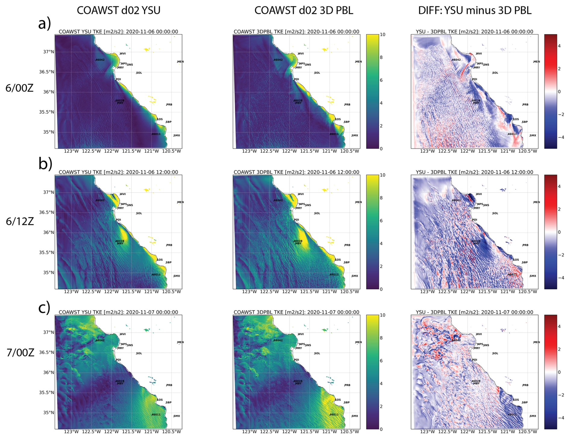
Figure 12 Instantaneous z=157 m plan views of the evolution of resolved plus SGS TKE over the ocean at (a) 00:00 UTC 6 November, (b) 12:00 UTC 6 November, and (c) 00:00 UTC 7 November. The left panel is the COAWST YSU simulation, the middle panel is the COAWST 3D PBL simulation, and the right panel is the difference field: YSU minus 3D PBL.

The resolved plus SGS TKE from the COAWST simulations was compared to TKE at the Morro Bay lidar buoy (obtained from velocity variance observations) and shown in Fig. 13. Prior to 12:00 UTC 6 November, both simulations had significantly more TKE aloft above z=150 m, and slightly more TKE near the surface. It is possible that the missing lidar observations between z=200–250 m were due to the cloud base. Both simulations captured the increased TKE near 12:00 UTC 6 November, but the magnitudes were weaker than observed. Both simulations predicted the secondary peak approximately 6 h ahead of the observations near 12:00 UTC 7 November.

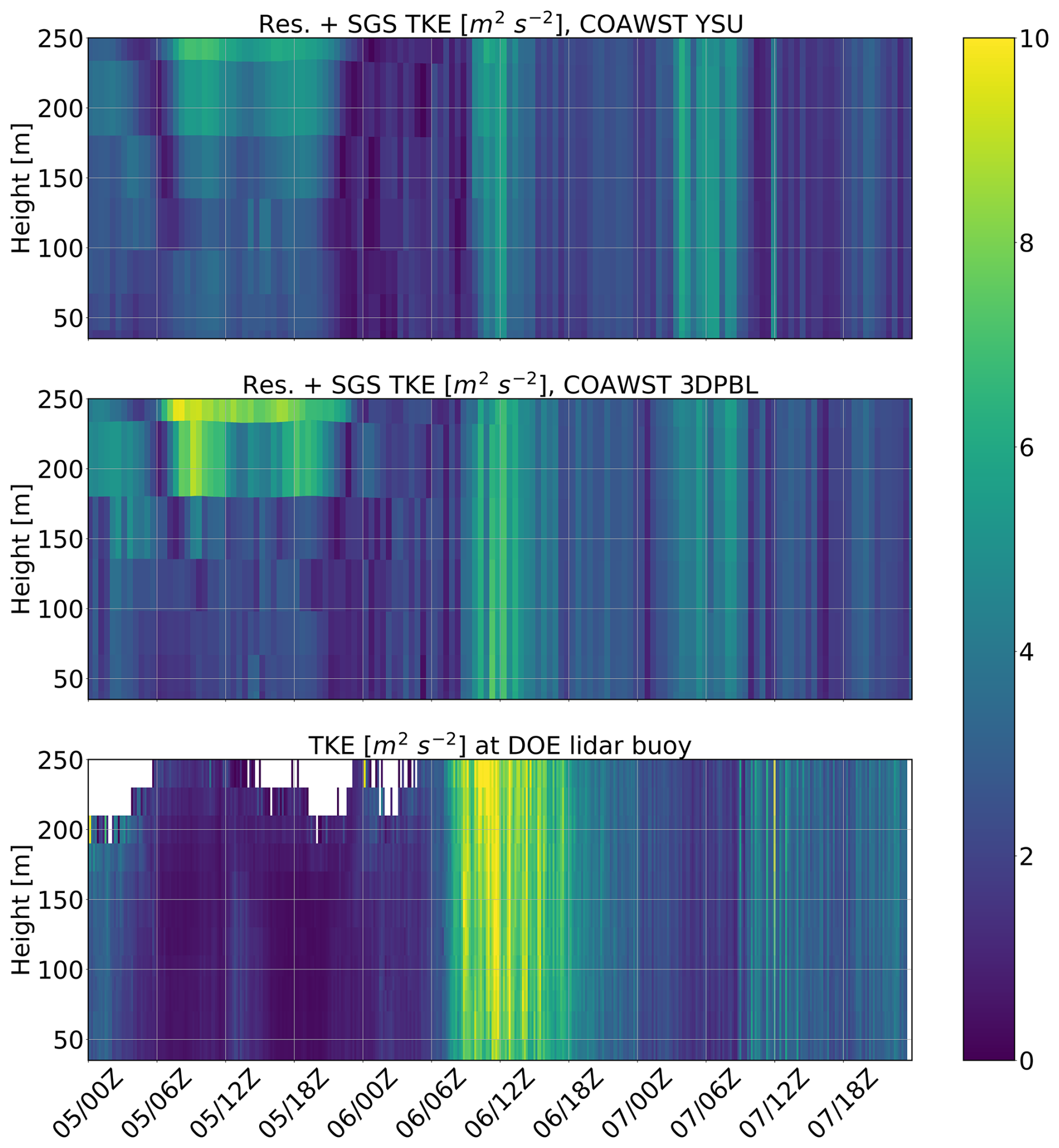
Figure 13 Time-height plot of TKE at the DOE Morro Bay lidar Buoy along with lidar buoy observations. Observations are 10 min averages and model time series are 10 min intervals. In the bottom panels, the white region denotes missing observations.

Finally, evolution of vertical profiles of winds and potential temperature are shown in Fig. 14. Prior to the frontal passage at 00:00 UTC 6 November, the wind speed peaked near z=200 m with a maximum around 15 m s⁻¹. The COAWST 3D PBL simulation matched the observations best at this time. The potential temperature profile showed a well-mixed boundary layer below z=150 m, with a strong inversion above. By 12:00 UTC 6 November, the boundary layer grew to z≈300 m, and the jet max moved upward to the boundary layer top with an increase in wind speed to approximately 25 m s⁻¹. Both simulations matched the lidar observations well below z=250 m. Finally, by 00:00 UTC 7 November, winds and temperature became very well mixed. The observed wind speeds were in between the COAWST YSU and 3D PBL simulations at this time.

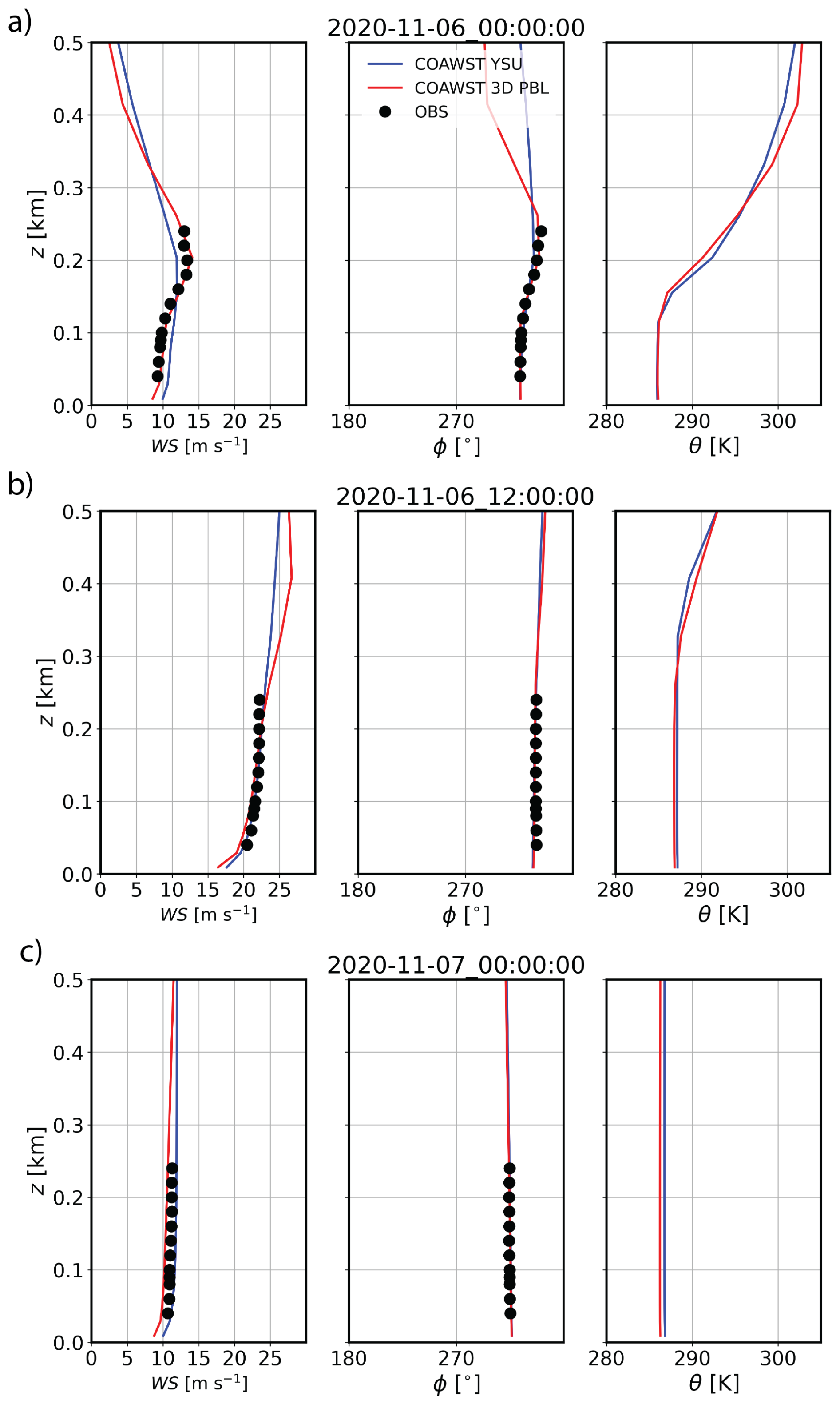
Figure 14 10-min mean model simulated vertical profiles and observations (black cirles). (a) 00:00 UTC 6 November, (b) 12:00 UTC 6 November, and (c) 00:00 UTC 7 November.

3.6 Synthesis of the observational evaluation

To summarize the observational evaluation in Sect. 3.4 and 3.5, both the COAWST YSU and COAWST 3D PBL compare favorably with near-surface buoys measurements and vertical wind profiles from the Morro Bay lidar (MBY). TKE in both simulations is slightly underestimated in comparison to MBY. Errors in wind speed for both simulations are generally larger over land. Both simulations predicted the gradual increase in significant wave height well, with the COAWST 3D PBL simulation producing slightly reduced wave heights, matching the observations better. Vertical profiles (Fig. 14) show the both simulations matched the observations well, with the COAWST 3D PBL simulation better producing the jet nose structure at 00:00 UTC 6 November than the COAWST YSU simulation.

3.7 Sensitivity test with the Mellor-Yamada 1D  PBL parameterization

A natural question that arises is to what extent are differences between the COAWST YSU and 3D PBL simulations due to the differences in vertical mixing treatment versus horizontal mixing treatment. Recall, the YSU parameterizaton uses a first-order, nonlocal, K-profile closure for SGS vertical mixing while the 3D PBL parameterization uses a 1.5-order, prognostic-TKE, local closure. Moreover, the YSU parameterization uses the 2D Smagorinsky parameterization in the horizontal directions while the 3D PBL parameterization does not. Therefore, a sensitivity test was carried out using the 1D version of the 3D PBL parameterization; a local, 1.5-order, prognostic TKE parameterization in the vertical direction (Mellor, 1973; Mellor and Yamada, 1974, 1982). This parameterization also uses the 2D Smagorinsky parameterization; therefore, the precise role of differences in the vertical mixing treatment between the YSU PBL parameterization and the 1D PBL parameterization can be understood. The instantaneous differences in the wave and 10 m wind fields between the COAWST 1D PBL and 3D PBL simulations (Fig. 15) are much smaller than the instantaneous differences between the COAWST YSU and 3D PBL simulations (Fig. 5). Therefore, most differences between the 3D PBL and YSU parameterizations are due to the differences in vertical mixing treatment, rather than differences between the 3D PBL parameterization's heteorogeneous treatment of the horizontal Reynolds stress and flux divergence terms and the 2D Smagorinsky parameterization. We note however, that it is possible that more differences in the horizontal mixing would be present if the full 3D PBL parameterization were used, and this will be explored in future work. Recall, in the full 3D PBL parameterization, gradients of mean quantities in the Mellor-Yamada level 2.5 mode are not neglected, leading to more realistic representation of SGS mixing.

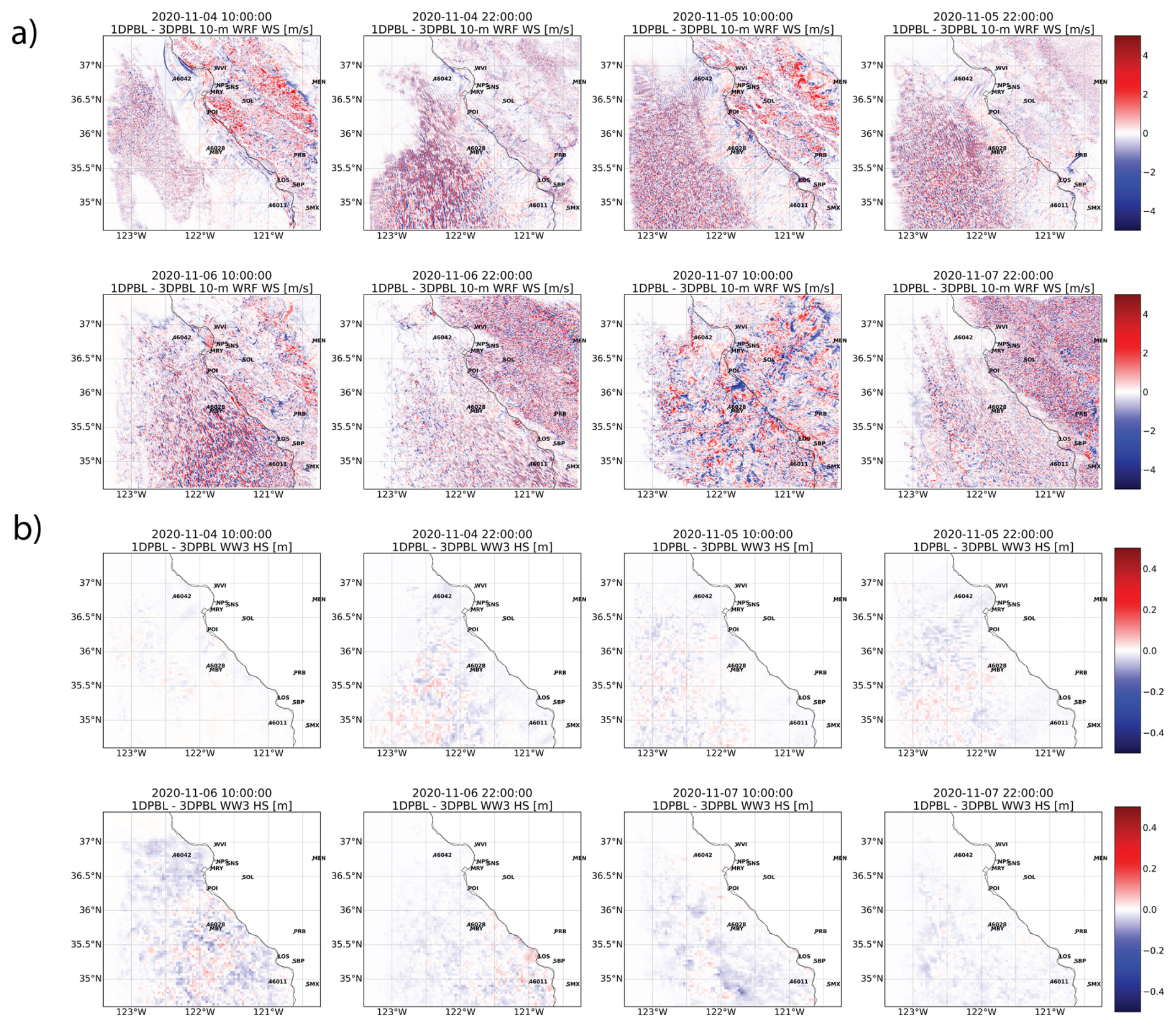
Figure 15 Instantaneous difference fields of (a) 10 m wind speeds (m s⁻¹) and (b) significant wave heights (m) every 12 h beginning on 10:00 UTC 4 November 2020. Difference is defined as the 1D PBL simulation minus the 3D PBL simulation.

4 Discussion and conclusions

Motivated by providing more realistic simulations of coastal flows relevant to offshore wind energy resource characterization, a 3D PBL parameterization was added to the coupled atmosphere/ocean/wave modeling system COAWST. Since the parameterization is designed for “gray zone” simulations, its functionality and utility were carried out using a high resolution coastal nest with Δx=400 m covering a large $\sim \mathrm{280}\times \mathrm{280}$ km geographic area containing the Bureau of Ocean Energy Management Morro Bay wind energy lease area. To rigorously evaluate the coupled 3D PBL parameterization under large variability in wind and wave conditions, a case study of a significant wind-wave event off the central California coast from 4–8 November 2020 was examined. Differences between COAWST simulations using a 1D (YSU PBL parameterization with a 2D Smagorinsky parameterization) and the approximated 3D PBL parameterization were examined, and both simulations were evaluated using observations over the ocean and land.

The main findings are as follows. Both the COAWST YSU and 3D PBL parameterization simulations were qualitatively similar in capturing both the peak of the wind and wave event, and both simulations matched buoy significant wave height and wind observations reasonably well. Wind speed mean absolute errors (MAEs) were approximately 1.1–1.7 m s⁻¹, wind direction MAEs were approximately 5–10°, and significant wave height MAEs were 0.4–0.6 m. Additionally, both simulations predicted the 2-m temperature and dewpoint well (MAEs of 0.5–0.8 °C, as well as accurately capturing the temperature and dewpoint decrease as the cold front passed (Fig. 7). The COAWST 3D PBL simulation had wind speed errors that were 0.02 m s⁻¹ less than the COAWST YSU simulation, and also a slight overall reduction in significant wave height errors (0.01–0.04 m). As the front passed between 06:00–18:00 UTC 6 November, the COAWST 3D PBL simulation predicted lower wave heights at NDBC buoys 46028 and 26011, more consistent with observations. The approximate 10 % lower wave heights predicted by the 3D PBL parameterization at the time of the frontal passage resulted from approximately 10 % lower 10 m wind speeds. The exact reasons for the wind speed differences between the YSU and 3D PBL simulation are not fully known, but they potentially result from the different treatment of vertical mixing. It is possible that nonlocal mixing in the YSU PBL parameterization during the convective conditions after the simulated frontal passage mixed higher momentum air downward, which was not captured as well as in the 3D PBL parameterization, which only accounts for vertical mixing in adjacent layers.

The simulated vertical profiles of winds and TKE were also compared to DOE Morro Bay lidar buoy observations. Both simulations compared favorably in terms of the timing of the increase in winds and TKE near 12:00 UTC 6 November. Vertical gradients in wind speed were captured prior to the frontal passage with stronger winds near the surface associated with the coastal low level jet, and well-mixed momentum after the frontal passage. The COAWST 3D PBL simulation better captured the vertical profile of the low level jet (“jet nose” structure) prior to the frontal passage.

Finally, by carrying out the first coupled wave/atmosphere simulations with the 3D PBL parameterization, we demonstrated that the parameterization can be used in a coupled modeling framework. In future work, we wish to execute coupled wave/atmosphere simulations using the full 3D PBL parameterization which would have improved treatment of horizontal mixing over the 3D PBL parameterization with the PBL approximation used here. Additionally, three-way (atmosphere, ocean, and wave) coupled simulations would further elucidate the impacts of the addition of ocean-atmosphere and ocean-wave coupling on differences between simulations using 1D and 3D PBL parameterizations.