Regional CO₂ and CH₄ inversion system using WRF-Chem (v4.4)/DART (v9.8.0) and continuous high-precision observations over the Korean Peninsula

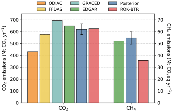
Quantifying greenhouse gas (GHG) emissions over complex terrain remains a significant challenge for conventional inversion systems due to the high sensitivity of tracer transport to surface heterogeneity. We develop a high-resolution dual-species GHG top-down inversion framework by integrating the Weather Research and Forecasting model coupled with Chemistry (WRF-Chem v4.4) and the Data Assimilation Research Testbed (DART v9.8.0) in a cycling ensemble Kalman filter system. Built on community tools, the framework is designed to be portable and configurable, enabling applications to other regions, resolutions, and observing-system configurations (e.g., expanded surface networks and additional data streams). This framework jointly assimilates near-surface CO₂ and CH₄ concentrations to produce dynamically consistent updates of emissions. By employing a unified Eulerian framework that simultaneously updates meteorology and 3-D tracer fields, the system is designed to maintain consistency between transport and concentrations and to reduce the risk that transport-related concentration errors are aliased into flux adjustments over the complex landscapes of the Korean Peninsula. To improve the simulation of turbulent GHG dispersion in the atmospheric boundary layer over complex terrain, we incorporate surface heterogeneity parameterizations (roughness sublayer and canopy height) into the model physics in the inversion system. The system assimilates high-precision continuous in situ observations from three World Meteorological Organization/Global Atmosphere Watch (WMO/GAW) stations to constrain CO₂ and CH₄ emissions. Prior flux estimates include anthropogenic emissions from the Emissions Database for Global Atmospheric Research (EDGAR v8.0), biogenic exchanges (the region-optimized Vegetation Photosynthesis and Respiration Model), biomass burning (Fire Inventory from the National Center for Atmospheric Research v2.5), and oceanic CO₂ exchanges (SeaFlux). In a 2020 case study, the top-down estimates improve the agreement with ground observations, reducing root-mean-square errors by 30 %–60 % and lowering posterior mean bias to 1–2 ppm for CO₂ and 20–30 ppb for CH₄ at the high-precision surface observation sites. Independent aircraft profiles provide external evaluation and indicate residual CH₄ discrepancies consistent with prior emissions and boundary condition uncertainties. Controlled observing-system simulation experiments show that, under prescribed perturbations, the system produces bounded and interpretable emission responses to transport-model, boundary-condition, and observation-error perturbations. They also indicate that recovery is strongest within station footprints and remains coverage-limited under the current three-station network, while a dense-network known-truth experiment highlights the value of expanded observational coverage for improving domain-wide emission constraints. Posterior adjustments suggest reduced CO₂ emissions over the Seoul Metropolitan Area and parts of the western coastal region and increased CH₄ emissions over inland agricultural source regions relative to the priors, highlighting priorities for follow-on evaluation of inventory components. Our posterior CO₂ total (620 ± 45 Mt yr⁻¹) is consistent with the Republic of Korea Biennial Transparency Report (ROK-BTR) estimate (624 Mt yr⁻¹) at the national scale, while the posterior CH₄ total (54.7 ± 5.2 Mt CO₂eq yr⁻¹) exceeds the ROK-BTR estimate (35.5 Mt CO₂eq yr⁻¹) by 19.2 Mt CO₂eq yr⁻¹, consistent with the larger structural uncertainty in CH₄ source characterization and spatial allocation noted in previous studies.

1 Introduction

Anthropogenic emissions of greenhouse gases (GHGs) originate predominantly from fossil fuel combustion, land-use change, agricultural practices, and waste management. These emissions are the principal drivers of contemporary climate change. Reliable and continuous monitoring of anthropogenic GHG emissions is essential for the development of effective climate mitigation strategies, compliance with international climate agreements, and the formulation of informed policy decisions (IPCC, 2021; Friedlingstein et al., 2025). Under the Paris Agreement, national inventories serve as the principal reporting mechanism, delineating Nationally Determined Contributions (NDCs) and facilitating periodic stocktakes (UNFCCC, 2015). These inventories are a standard method within the Measurement, Monitoring, Reporting, and Verification (MMRV) framework and rely on bottom-up methodologies based on activity data and emission factors within a tiered framework established by the Intergovernmental Panel on Climate Change (IPCC) (Ogle et al., 2013). However, their accuracy is often limited by incomplete or outdated activity data, coarse spatio-temporal resolution, diffusive GHG emissions, and systemic delays in updating or reporting inventories (Rogelj et al., 2016; Pauw et al., 2018). Even nations with advanced inventories encounter challenges in capturing rapid emission changes, fine-scale spatial heterogeneity, and localized sources, which undermine the inventory credibility and comparability of inventories (Denison et al., 2019; Nisbet et al., 2019; WMO, 2025).

Top-down approaches, which are based on atmospheric inverse modeling or atmospheric data assimilation (DA), offer independent assessments of emissions by constraining surface fluxes through atmospheric concentration measurements (Enting, 2002; Gurney et al., 2002; Weiss and Prinn, 2011; Oda et al., 2019; Janssens-Maenhout et al., 2020; Elguindi et al., 2020; Mueller et al., 2021; Deng et al., 2022; WMO, 2025). These methodologies are increasingly incorporated into MMRV frameworks (WMO, 2022, 2025). By reconciling observed atmospheric concentrations with emission fluxes, top-down approaches can identify unreported or misrepresented emission sources, detect biases, and provide spatially explicit, policy-relevant emission information (Janssens-Maenhout et al., 2020; Mueller et al., 2021). Recent advancements in observational infrastructure, including dense atmospheric observation networks, satellite platforms, and airborne measurements, have enabled top-down systems to resolve emission patterns at urban and sub-national scales, thereby enhancing the fidelity and applicability of MMRV systems (Lauvaux et al., 2020; Byrne et al., 2023; Velasco et al., 2023).

Atmospheric inverse modeling frameworks for GHGs differ in how they numerically represent tracer transport. Lagrangian-based approaches release virtual air parcels at receptor sites and track their trajectories backward through prescribed wind fields, reconstructing source-influence functions from the particle paths (e.g., Henne et al., 2016; Pisso et al., 2019; Sijikumar et al., 2023; Brunner et al., 2025; Bukosa et al., 2025). Eulerian approaches instead solve the advection–diffusion continuity equation for tracer mixing ratios on a fixed spatial grid. Within the Eulerian class, global offline systems advect tracers through reanalysis wind, convective mass-flux, and boundary-layer depth fields supplied at each integration step, while regional online-coupled systems such as WRF-Chem integrate the meteorological state and the tracer fields through a single numerical framework, applying the same advection operators, turbulence closures, and planetary-boundary-layer scheme to both. Representation errors in boundary-layer dynamics and sub-grid mixing have been documented across inversion configurations in which meteorology and tracer transport are treated through separate numerical pipelines (Bréon et al., 2015; Lauvaux et al., 2016; Dekker et al., 2017; Super et al., 2017; Gaudet et al., 2021; Nalini et al., 2022; Bukosa et al., 2025). Online-coupled integration yields temporal and sub-grid consistency between the resolved flow and the simulated GHG evolution, which is particularly suited to ensemble-based DA techniques (Kang et al., 2012; Gaudet et al., 2021), including the Ensemble Adjustment Kalman Filter (EAKF) (Anderson, 2001, 2003).

These considerations motivate the development and documentation of complementary high-resolution Eulerian DA frameworks that can explicitly represent mesoscale transport and boundary-layer mixing over heterogeneous surfaces and can be extended to future dense observing systems. The Weather Research and Forecasting model coupled with Chemistry (WRF-Chem) provides high-resolution, online coupling of meteorology and chemistry, while the Data Assimilation Research Testbed (DART) offers an ensemble-based DA platform for dynamically updating meteorological and chemical states. Accordingly, WRF-Chem coupled with the DART has been used in CO₂ concentration, regional meteorology and air quality studies (e.g., Mizzi et al., 2018; Ma et al., 2020; Zhang et al., 2021a). Previous studies have demonstrated the feasibility of coupling WRF-Chem with DART for CO₂ flux inversion using satellite XCO₂ retrievals in an ensemble Kalman filter framework (Zhang et al., 2021a, b; Jin et al., 2025).

While these studies establish feasibility, they have primarily focused on single-species CO₂ estimation constrained by intermittent satellite sampling, and the extent of independent flux evaluation (e.g., using independent in situ/aircraft constraints) and controlled sensitivity testing remains relatively limited for robust flux-inversion assessment. Furthermore, applications to CO₂ and CH₄ regional inversions at kilometer-scale transport resolution remain limited particularly in complex-terrain environments where transport–flux aliasing and representativeness errors can be substantial. To our knowledge, a fully documented WRF-Chem/DART regional inversion framework that simultaneously targets CO₂ and CH₄ emissions and assimilates both in situ GHG observations and meteorological fields within a cycling dual-state configuration has not yet been documented in the literature. The present study fills this gap by providing a reproducible dual-species (CO₂ $/$ CH₄) state-augmentation system with explicit configuration choices, including uncertainty assumptions, localization/inflation, observation selection, boundary condition handling, together with a real-data application and a supplementary set of controlled Observing System Simulation Experiments (OSSEs) spanning transport-model, boundary-condition, and representativeness errors and real case tests on consistency of ensemble member and spread.

Here we extend the WRF-Chem (v4.4) and DART (v9.8.0) framework to implement a 9 km dual-species inversion system that cycles meteorological DA while assimilating near-surface CO₂ and CH₄ observations, directly updating meteorology and 3-D tracer fields and estimating surface flux adjustments through ensemble cross-covariances. We further incorporate surface-heterogeneity-related physics and land information (e.g., roughness-sublayer and canopy-height adjustments) tailored to the Korean Peninsula, where complex topography, coastal circulations, clustered emissions, and monsoon seasonality pose challenges for conventional inventories and coarse-resolution inversions (e.g., Hong and Kim, 2011; Hong et al., 2019; Hong et al., 2020; Lee et al., 2021; Kim et al., 2024). The main practical assessment is based on the 2020 real-data application, using concentration-space diagnostics, flux uncertainty reduction, independent aircraft observations, and intercomparisons with multiple emission datasets to evaluate the framework's relevance for future national MMRV-oriented applications.

2 Description of CO₂ and CH₄ inversion framework

2.1 Atmospheric modeling system

Our GHG inversion framework integrates a regional Eulerian atmospheric chemistry model with an ensemble-based data assimilation system. Specifically, this framework employs the Weather Research and Forecasting model coupled with Chemistry (WRF-Chem v4.4; Grell et al., 2005) and the Data Assimilation Research Testbed (DART v9.8.0) (Anderson et al., 2009) for sequential data assimilation. WRF-Chem solves the fully compressible, nonhydrostatic Eulerian equations on a fixed spatial grid, and simulates atmospheric dynamics, physical and chemical processes, and chemical transport within a unified framework.

In the inversion system, WRF-Chem generates ensemble forecasts by simulating meteorology with surface fluxes and atmospheric transport processes of GHGs. Given the long atmospheric lifetime of GHGs, they have been simulated as passive tracers in mesoscale models (Dekker et al., 2017; Super et al., 2017; Zhao et al., 2023). WRF-Chem includes the module to simulate passive tracer transport of GHGs since WRF-Chem v3.4 (Beck et al., 2012). In WRF-Chem, distinct variables represent background, anthropogenic, biomass-burning, oceanic (CO₂ only), and biogenic components of CO₂ and CH₄. The model simulates their fluxes, transport, and diffusion processes driven by the meteorological field to obtain a three-dimensional concentration field on an hourly basis. The total concentrations are represented as the sum of the component variables, facilitating comparison with observed concentrations. CO₂ and CH₄ are treated as passive tracers for our regional application because the relative chemical lifetime of CH₄ against OH is on the order of years (about 9 years), whereas typical air-mass residence times across our regional domain are < 1 d (Zhao et al., 2020; Callewaert, 2024). Therefore, the implied fractional loss is negligible compared to transport and emission uncertainties. In addition, large-scale chemical aging and seasonality are already reflected in the prescribed initial and lateral boundary conditions.

Our study area consists of a single model domain with 9 km horizontal spacing of 97×136 grid points and 51 terrain-following vertical levels stretching from the surface up to 50 hPa at the upper boundary (Fig. 1). The model employed specific physics parameterization schemes (Kim et al., 2024 and references therein), including the WSM-6 microphysics, Rapid Radiative Transfer Model for General Circulation Models (RRTMG) shortwave and longwave radiation schemes, the Yonsei University scale-aware Planetary Boundary Layer (PBL) scheme, Kain-Fritsch cumulus scheme, and the Unified Noah Land Surface Model (LSM).

Notably, for better simulations of GHG transport over complex terrain, we used the revised WRF-Chem by replacing the default WRF canopy height with high-resolution (1 km) spaceborne lidar-retrieved canopy height data (GLAS/ICESat) for a better representation of surface characteristics (Lee and Hong, 2016). To simulate realistic transport and dispersion of GHG in the PBL, we further adapted roughness sublayer (RSL) parameterization of Lee et al. (2020), which incorporated the RSL function from the unified theory of Harman and Finnigan (2007, 2008) and Harman (2012), into the revised MM5 surface layer scheme (Jiménez et al., 2012) and Unified Noah LSM in WRF. Hereafter, we refer to this modified WRF-Chem v4.4 as WRF-Chem GHG.

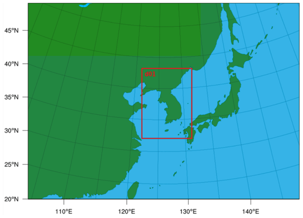
Figure 1 The WRF-Chem model domain used in this study. The red rectangle, marked d01, is the single computational domain of the WRF-Chem simulation (9 km horizontal spacing, 97 × 136 grid points), covering the Korean Peninsula and its surrounding seas. The remainder of the map shows the wider East Asian region for geographic context and is not part of the simulated area.

2.2 DART data assimilation for GHG inversion

DART serves as a modular DA system designed to interface with various atmospheric models and observational datasets. The integration of WRF-Chem and DART enables the simultaneous assimilation of meteorological variables and chemical species through multivariate, dynamically consistent updates across the coupled system (Mizzi et al., 2016, 2018). The system operates as an ensemble of WRF-Chem forecasts, where each member represents a perturbed version of the state vector that accounts for both observational and model uncertainties. At each analysis cycle, ensemble perturbations are utilized to estimate a flow-dependent background error covariance, enabling the EAKF to adjust both meteorological and tracer fields simultaneously in a dynamically balanced manner. This ensemble-based structure allows for uncertainty propagation, sequential updating of the background (prior) ensemble, and the maintenance of consistency between state variables during sequential assimilation. Hereafter, we refer to WRF-Chem GHG coupled with DART as WRF-Chem/DART.

Our work extends the DA system to facilitate the simultaneous assimilation of observed CO₂ and CH₄ concentrations with meteorological data at a spatial resolution of 9 km over the Korean Peninsula. The assimilated data include continuous in situ CO₂ and CH₄ concentrations, together with standard global upper-air and surface meteorological observations from the National Centers for Environmental Prediction (NCEP) provided in the prepared Binary Universal Form for the Representation of meteorological data (PREPBUFR) format. Because meteorology is simulated and updated within the online WRF-Chem/DART cycling system (rather than prescribed as offline transport fields), the inversion does not rely on externally prescribed meteorological trajectories. Meteorological initial and boundary conditions (IC/BCs hereafter) are provided from standard large-scale reanalysis products as in limited-area modeling.

We use an ensemble size of 20 members throughout the cycling assimilations in the WRF-Chem/DART system. A real-case simulations with 10, 20, and 30 members show that the 20- and 30-member configurations behave similarly with the reliable prior RMSE/total-spread ratio, supporting the 20-member choice as a practical compromise between covariance sampling and computational cost (Supplement Sect. S3.1, Fig. S23). The analysis directly updates the prognostic meteorological variables and 3-D tracer concentration fields each cycle, while emission adjustments are estimated as surface forcing parameters for the subsequent forecast, rather than being dynamically transported like tracer concentrations. This cycling approach helps preserve meteorology–transport–concentration consistency between the analyzed meteorology/tracer fields and the subsequent model transport in the ensemble forecasts. In the sequential EAKF framework, correcting the tracer concentration state at each analysis step (e.g., using the analysis field as the initial condition for the subsequent forecast) helps prevent the carry-over of transport-driven concentration biases and reduces the risk that these biases are aliased into inferred emission adjustments. As demonstrated in previous WRF-Chem/DART studies (Liu et al., 2017; Hsu et al., 2024), failure to correct the concentration state allows transport-driven biases to persist into subsequent forecast steps. The filter would then continuously interpret these persistent concentration residuals as evidence of flux errors, leading to the artificial amplification of emission estimates (over-adjustment) to compensate for accumulated biases. For passive tracers such as CO₂ and CH₄, chemical loss is negligible at the cycling timescale, so transport-driven biases accumulate without meaningful attenuation. Similar concentration-state correction is applied in ensemble-based CO₂ flux estimation systems (Kang et al., 2011, 2012; Peng et al., 2015). By updating the concentration state at each cycle, the system ensures that emission adjustments are derived primarily from mismatches between model forecast and observation within the current assimilation window.

We implement this joint state–emission estimation using a state-augmentation approach in DART (Kang et al., 2011, 2012; Liu et al., 2017; Zhang et al., 2021a; Huang et al., 2022). The augmented state vector is defined as

$$\begin{array}{}\text{(1)}& \mathit{z}\equiv \mathit{x}={\left[{\mathit{x}}_{\mathrm{met}},{\mathit{x}}_{\mathrm{chem}},{\mathit{x}}_{\mathrm{flux}}\right]}^T\end{array}$$

where x_met contains meteorological variables including zonal and meridional wind, temperature, specific humidity, and surface pressure ($U,V,T,Q,$ and P_sfc respectively), x_chem contains three-dimensional CO₂ and CH₄ mixing ratios, and x_flux contains two-dimensional surface emission flux fields and is represented as time-indexed (e.g., hourly) flux fields that are applied as external surface-forcing inputs to WRF-Chem during the subsequent forecast integration. At each analysis time, the deterministic EAKF updates the prior (background) augmented-state ensemble to the posterior ensemble as Eqs. (2), (3), (4)

$$\begin{array}{}\text{(2)}& {\displaystyle }\stackrel{\mathrm{‾}}{{\mathit{z}}^u}={\mathbf{\Sigma }}^u\left[{\left({\mathbf{\Sigma }}^p\right)}^{-\mathrm{1}}\stackrel{\mathrm{‾}}{{\mathit{z}}^p}+{\mathbf{H}}^T{\mathbf{R}}^{-\mathrm{1}}{\mathit{y}}^{\mathrm{o}}\right]\text{(3)}& {\displaystyle }{\mathbf{\Sigma }}^u={\left[{\left({\mathbf{\Sigma }}^p\right)}^{-\mathrm{1}}+{\mathbf{H}}^T{\mathbf{R}}^{-\mathrm{1}}\mathbf{H}\right]}^{-\mathrm{1}}\text{(4)}& {\displaystyle }{\mathit{z}}_i^u=\mathbf{A}\left({\mathit{z}}_i^p-\stackrel{\mathrm{‾}}{{\mathit{z}}^p}\right)+\stackrel{\mathrm{‾}}{{\mathit{z}}^u},i=\mathrm{1},\mathrm{\dots },N\end{array}$$

where $\stackrel{\mathrm{‾}}{{\mathit{z}}^u}$ and $\stackrel{\mathrm{‾}}{{\mathit{z}}^p}$ denote the posterior and prior ensemble means, respectively. The subscript i in ${\mathit{z}}_i^p$ and ${\mathit{z}}_i^u$ indicates the ith member of the prior/posterior ensembles, and N is the ensemble size. y^o is the observation vector including in situ CO₂ $/$ CH₄ and PREPBUFR meteorological observations, R is the observation-error covariance matrix, and H is the corresponding observation (forward) operator. Σ^p and Σ^u are the prior and posterior error covariance matrices, respectively. A is a transformation matrix satisfying Σ^u=AΣ^pA^T, consistent with the EAKF adjustment used here. Equations (2) and (3) provide a compact summary of the linear Kalman analysis. In practice, DART implements the EAKF as a deterministic, serial ensemble update in observation space, where each observation is assimilated sequentially using ensemble-estimated covariances with covariance localization. The ensemble adjustment matrix A in Eq. (4) is computed so that the posterior ensemble anomalies reproduce the localized posterior covariance in Anderson (2001, 2003), thereby avoiding the sampling noise associated with stochastic perturbations of observations. We refer to Anderson (2001, 2003) and Anderson et al. (2009) for the detailed mathematical and theoretical backgrounds for EAKF.

For in situ CO₂ and CH₄, we specify the observation error variance as ${\mathit{\sigma }}^{\mathrm{2}}={\mathit{\sigma }}_{\mathrm{meas}}^{\mathrm{2}}+{\mathit{\sigma }}_{\mathrm{repr}}^{\mathrm{2}}$, where ${\mathit{\sigma }}_{\mathrm{meas}}^{\mathrm{2}}$ is the measurement uncertainty reported for the WMO/GAW stations (Lee et al., 2019; Lee et al., 2023) and ${\mathit{\sigma }}_{\mathrm{repr}}^{\mathrm{2}}$ is treated as a model–data mismatch term, not as an instrument error, and its magnitude is chosen to maintain stable cycling behavior and to avoid overfitting sparse point observations in a 9 km grid framework. Because ${\mathit{\sigma }}_{\mathrm{meas}}^{\mathrm{2}}$ is expected to be small for WMO/GAW-quality observations, ${\mathit{\sigma }}_{\mathrm{repr}}^{\mathrm{2}}$ is treated as the primary contributor and is parameterized as a concentration-proportional term (as 5 % of the observed mole fraction) across all sites. This results in a relatively large effective error variance (typically ∼ 20 ppm for ambient CO₂ and ∼ 100 ppb of CH₄). This conservative parameterization is chosen not only to account for sub-grid variability but also to maintain analysis stability given the sparsity of the operational network. In data-sparse regions, relying too heavily on individual stations (via small observation errors) risks introducing spurious emission artifacts driven by local transport transients; a larger error specification mitigates this risk by ensuring that increments are driven only by persistent, robust signals. For PREPBUFR meteorological observations, we use the DART default observation error specifications based on the NCEP operational error tables (e.g., rawin wind: 1.4–3.2 m s⁻¹, radiosonde temperature: 0.8–1.5 K, land station wind: 3.5 m s⁻¹, marine wind: 2.5 m s⁻¹, surface pressure: 1.0 hPa), which are platform- and pressure- (altitude) dependent. The synthetic-observation errors used in the controlled OSSEs are specified separately in Supplement file S2 to impose prescribed observation-error perturbations of known magnitude; they are therefore controlled sensitivity settings rather than a direct restatement of the real-data representativeness-error parameterization.

Although the surface emission fluxes x_flux are not directly observed (i.e., H has no sensitivity to fluxes), they are updated through the ensemble cross-covariances Cov(x_chem,x_flux). These flow-dependent covariances enable statistically consistent flux adjustments that reduce concentration innovations, provided that physically plausible concentration–flux relationships exist within the localization radius. The updated emission fields are prescribed as static surface inputs that persist during the subsequent forecast window, rather than being advected as prognostic variables. Thus, the emission corrections obtained at each analysis cycle propagate forward through the forecast into the next analysis cycle. To suppress sampling error and spurious long-range correlations, we apply covariance localization using a Gaspari–Cohn polynomial (Gaspari and Cohn, 1999) with a horizontal half-width of 0.025 rad (∼ 160 km) and a vertical normalization cutoff radius of 1.5 km, constraining increments primarily to the lower troposphere and reducing under-sampling error (Anderson, 2012; Kang et al., 2012). Cross-species covariances are not applied; CO₂ and CH₄ tracers are updated independently. To mitigate ensemble under-dispersion, we apply adaptive prior inflation in DART (inf_flavor = 2). The inflation standard deviation is initialized at 0.6 and damped by a factor of 0.9, with the maximum allowed change per cycle limited to 1.05. A real-case comparison of three adaptive-inflation configurations (prior-only and prior-and-posterior Gaussian schemes, and a prior-only inverse-gamma scheme) yields nearly identical prior RMSE-to-spread ratios at the observation sites, indicating that the concentration-space spread consistency under the tested configurations (Fig. S24).

Prior uncertainty is represented by applying Gaussian, multiplicative perturbations to the chemical initial state, lateral boundary conditions, and anthropogenic emission fluxes when generating the forecast ensemble. For each ensemble member, perturbation factors are drawn from normal distributions centered at unity, with 1σ standard deviations of 5 % for chemical initial and lateral boundary conditions and 30 % for anthropogenic fluxes. The former represents a pragmatic balance between acknowledging residual uncertainty in the reanalysis inflow and preventing ensemble over-spreading that would overwhelm regional increments, while the latter is chosen to span the inter-inventory discrepancies over the Korean Peninsula (see Sect. 6.4 for details). The initial error configurations also align with those from previous studies (e.g. Zhang et al., 2021a, b). Horizontal and vertical correlation lengths are specified as 200 and 1 km, respectively.

Analyses are produced every six hours (00:00, 06:00, 12:00, 18:00 UTC) using observations within a ±3 h window centered on the analysis time; observations are rejected if they exceed three standard deviations of the background ensemble. The resulting analyzed ensemble is then advanced with WRF-Chem to provide the background for the next cycle, updating the chemical and meteorological initial conditions accordingly. To maintain dynamical consistency near the domain boundaries, the analysis increments are propagated consistently into the lateral boundary tendencies used for the subsequent forecast, preventing spurious discontinuities at the boundary interface. This is a numerical continuity treatment and does not constitute an independent optimization of boundary inflow.

A controlled evaluation of the inversion is provided in Supplement file S2. It first presents an error-source matrix (Sect. S1) in which the control known-truth retrieval (CTL) serves as the baseline, and prescribed perturbations are introduced for transport-model error, boundary-condition bias, observation-error/representativeness sensitivity, localization radius, and their combination (Table S2, Figs. S15–S19) (Michalak et al., 2017; Bisht et al., 2023). These experiments are controlled diagnostics of the implemented state-augmentation system rather than demonstrations of real-world flux accuracy. Under the tested perturbations, the system produces bounded and interpretable emission responses: the structural-error experiments change the domain-mean recovery by less than about 2 percentage points of the prior, whereas the localization sweep produces somewhat larger but still bounded changes. Supplement file S2 then presents a separate dense-network known-truth experiment as an idealized information-content diagnostic for expanded observational coverage (Sect. S2), and provides real-case diagnostics of ensemble-size and inflation-configuration sensitivity (Sect. S3). Together, these tests characterize the current configuration, identify coverage-limited recovery as a key uncertainty, and motivate future observing-system expansion and assimilation-window sensitivity tests.

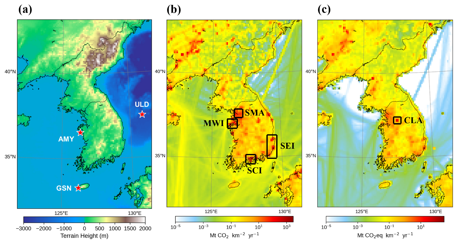
Figure 2 Locations of GHG monitoring stations (AMY, GSN, ULD) over terrain height (a) and annual anthropogenic emissions of CO₂ (b) and CH₄ (c) in the model domain in 2020 from the Emissions Database for Global Atmospheric Research (EDGAR v8.0). Main emission source regions in the model domain are boxed: SMA (Seoul Metropolitan Area), MWI (Mid-Western Industrial Area), SEI (Southeastern Industrial Area), SCI (South Coast Industrial Area), and CLA (Central Livestock Area).

3 Observation data of GHG concentrations and meteorological conditions for data assimilation

High-precision, continuous ground-based GHG measurements are essential for capturing high-frequency variability and providing constraints on regional enhancements near major source regions. To constrain CO₂ and CH₄ fields, the inversion framework assimilates in situ measurements of CO₂ and CH₄ concentrations from the WMO/GAW-affiliated monitoring stations at Anmyeondo (AMY), Gosan, Jeju Island (GSN), and Ulleungdo (ULD) operated by the Korea Meteorological Administration (KMA) (Fig. 2a). Depending on wind direction and atmospheric stability, these sites measure background inflow and downwind plumes from key emission source regions (Fig. 2b and c). We therefore retain pollution events (no background selection) and rely on the coupled transport and localization to attribute information primarily within these key source regions.

Each site employs a harmonized measurement system based on cavity ring-down spectroscopy (CRDS, Picarro Inc., USA), paired with a custom cryogenic drying system jointly developed by KMA and the Korea Research Institute of Standards and Science. This setup ensures high-precision CO₂ and CH₄ measurements with minimal water vapor interference, critical for ensuring data quality under Korea's seasonally variable meteorological conditions. Data are collected at 1 min intervals, processed hourly into Level-2 quality-assured products. Here, Level-2 denotes QA/QC screening and calibration processing, distinct from “background-selected” products that apply additional baseline selection. All stations are operated as GAW monitoring stations with documented QA/QC and are used here to constrain regional-scale enhancements rather than micro-scale local fluxes. It is worth noting that this Level-2 dataset excludes instrumental artifacts (e.g., calibration periods) but retains local and regional pollution events without applying background selection filters, ensuring that the high-concentration signals required for regional inversion are preserved. Further details on instrument calibration, QA/QC protocols, and traceability to international standards for CO₂ and CH₄ observations at WMO/GAW sites in Korea can be found in Lee et al. (2019) and Lee et al. (2023), respectively.

The new surface parameterizations adopted in this study improve wind simulations near the surface (e.g., Lee et al., 2015; Lee and Hong, 2016; Lim et al., 2019; Lee et al., 2020; Lee et al., 2023; Kim et al., 2024; Jo et al., 2025; WMO, 2025). For reference, we provide concise verification of modeled 10 m winds with KMA's Automated Synoptic Observing System (ASOS) observations at Seosan (∼ 32 km NNE of AMY), ULD, and GSN, complemented by a comparison against the marine meteorological observation buoy ∼ 18 km east of ULD (Figs. S1–S2 and Table S1). At ULD (a steep volcanic island in open ocean, ∼73 km² in area with a peak rising to ∼ 984 m, comparable in extent to a single grid cell), the model exhibits relatively large wind errors that the grid cannot fully resolve; the buoy comparison shows substantially better model agreement with the surrounding marine wind field, while indicating a possible discrepancy related to local topographical representativeness rather than systematic regional transport bias.

In addition, we assimilate conventional meteorological observations from the NCEP PREPBUFR datasets. These include surface pressure, near-surface air temperature, wind speed and direction, and specific humidity, as well as sea surface temperature and upper-air wind observations (including satellite-derived winds, radiosonde soundings, and aircraft reports of winds, temperature, and humidity). Assimilating these data effectively constrains the meteorological state (winds, temperature, and humidity), thereby improving transport fidelity in the coupled WRF-Chem/DART system, consistent with the previous applications (Mizzi et al., 2016, 2018; Pouyaei et al., 2023).

4 Initial and boundary conditions for meteorological variables and GHG concentrations

Meteorological initial and boundary conditions are obtained from the hourly ERA5 global reanalysis data at 0.25° × 0.25° resolution (Hersbach et al., 2020, 2023a, b). The initial and boundary conditions are preprocessed by the WRF Preprocessing System (WPS) to the model grid and then perturbed by the WRF Data Assimilation System (WRFDA), as described in previous studies (Barker et al., 2012; Mizzi et al., 2016; Liu et al., 2017; Zhang et al., 2021b).

Initial and boundary conditions of CO₂ and CH₄ are provided by the ECMWF CAMS global GHG reanalysis (EGG4 hereafter) data (Inness et al., 2019; Agustí-Panareda et al., 2023). EGG4 applies 4D-Var data assimilation of in situ networks and satellite retrievals within the ECMWF's Integrated Forecast System (IFS Cycle 47R1) and currently covers the period of 2003–2020. The dataset provides atmospheric mixing ratios of CO₂ and CH₄, along with meteorological and chemical variables on regular 0.75° × 0.75° grid in 25 pressure levels and 60 hybrid σ-pressure vertical levels at 3-hourly intervals. EGG4 data as initial and lateral boundary conditions help ensure that large-scale seasonal and regional variability and the growing season CO₂ drawdown are represented in the background fields.

Previous evaluations indicate that EGG4 reanalysis data may exhibit systematic biases. Overall errors in CO₂ and CH₄ concentrations are within 10 ppm and 40 ppb near the Earth's surface (Agustí-Panareda et al., 2023). Validation of EGG4 data against Total Carbon Column Observing Network (TCCON) measurement shows standard deviations of the difference of 1.18 ppm for XCO₂ and 11.3 ppb for XCH₄ (Wang et al., 2023). Notably, it has been reported that EGG4 data have a positive bias of CO₂ concentrations in high-emission regions, and its mean bias is about 7.46 ppm in Asia (Custódio et al., 2022). Regional biases can be systematic and location-dependent; for example, a negative bias of about 30 ppb in CH₄ concentration has been reported at the NOAA flask site in the midwestern industrial region (MWI) (Segato et al., 2025). We also note that even though EGG4 accounts for large-scale CH₄ oxidation, it relies on prescribed OH fields (or climatological loss rates) rather than interactive chemistry. This parameterized sink can introduce systematic errors in CH₄ concentrations, where the prescribed loss rates fail to capture local and temporal variability in photochemical destruction (e.g., Zhao et al., 2020; Agustí-Panareda et al., 2023). We summarize these boundary-driven bias characteristics as diagnostic context to motivate our boundary-condition uncertainty treatment and to aid the interpretation of residual baseline behavior discussed in Sect. 6.

5 Prior fluxes

5.1 Anthropogenic emissions

Within the domain, WRF-Chem simulates GHG transport and adds contributions from local surface emissions and sinks. Anthropogenic CO₂ and CH₄ emissions used as prior fluxes are regridded from the EDGAR global GHG emission inventory version 8.0 (Crippa et al., 2023). EDGAR provides anthropogenic emissions data in accordance with IPCC-compliant methodologies based on international activity data and emission factors (Janssens-Maenhout et al., 2019; Crippa et al., 2024). In EDGAR, the sectoral composition differs markedly between CO₂ and CH₄ over South Korea. CO₂ emissions are dominated by the power, energy, and industrial sectors (combustion and processes), with additional contributions from transport, fuel exploitation, and buildings (and minor contributions from remaining sources). In contrast, CH₄ emissions are dominated by agriculture and waste, followed by fuel exploitation, while other sectors are comparatively minor. It is also worth noting that wetland-like CH₄ emissions from rice paddies are categorized under the anthropogenic agricultural sector in EDGAR and are therefore included in our prior emissions. The inventory data used in this study, EDGAR, does not include natural wetland methane emissions and it is reported that annual CH₄ emission from natural wetlands in Korea is about 0.001–0.01 Tg CH₄ (Zhang et al., 2025). This is less than 0.5 % of the national total anthropogenic CH₄ emissions.

Annual spatial distributions of CO₂ and CH₄ emissions across the domain are shown in Fig. 2. To consider temporal variability in CO₂ emissions by human activities and disaggregate to hourly emissions, we apply the monthly and diel scaling factors reported by the EDGAR and the gridded Temporal Improvements for Modelling Emissions by Scaling (TIMES) factors, respectively. These account for building heating/cooling usage patterns, traffic volume fluctuations, sectoral contributions (residential, commercial, transportation emission), and weekday-weekend differences at 0.25°×0.25° resolutions (Nassar et al., 2013). Over ocean grid cells, EDGAR emissions are near zero except along major shipping lanes (if included in the selected EDGAR sectors). For CH₄ anthropogenic emissions, no diurnal TIMES disaggregation is applied; temporal variation is retained at the monthly level.

The spatial distributions of annual anthropogenic CO₂ and CH₄ emissions highlight the main source regions within the model domain (Fig. 2b and c). Strong CO₂ emissions in the Seoul Metropolitan Area (SMA) reflect aggregated contributions from power plants, traffic, and building emissions in the urban area. Industrial processes and power generation dominate emissions in the MWI and south and southeastern coast industrial corridors (SCI and SEI) over the Korean Peninsula (Fig. S3). CH₄ sources are generally coincident with strong CO₂ emission regions due to waste management in highly populated area but exhibit more spatially confined peaks with hotspots over the high-density urban area (SMA) (wastewater and landfills) and central livestock area (CLA) (enteric fermentation and manure management) (Fig. S4).

5.2 Biomass burning emissions

Biomass burning emissions of CO₂ and CH₄ are taken from the Fire Inventory from the National Center for Atmospheric Research (NCAR) (FINN version 2.5). This dataset estimates biomass burning emissions using burned-area calculations, year-specific land cover and vegetation datasets, fuel loading and emission factors, and the use of multiple fire-detection satellites, such as MODerate resolution Imaging Spectroradiometer (MODIS) and Visible Infrared Imaging Radiometer Suite (VIIRS) (Schroeder et al., 2014). FINN provides emissions at 1 km spatial resolution and daily temporal resolution (Wiedinmyer et al., 2011; Callewaert et al., 2022; Wiedinmyer et al., 2023). The NCAR fire-emission preprocessing tool is used to subset the inventory over the modeling domain, regrid it to the model grid, and temporally disaggregate it to hourly emissions for WRF-Chem GHG simulations. Biomass burning emissions show strong spatial and seasonal variability in our domain (Fig. S5 for CO₂ and Fig. S6 for CH₄). Seasonal enhancements are primarily observed in spring (March–May), possibly related to agricultural residue burning and land-clearing practices. The total contribution of biomass burning emissions over the Korean Peninsula is negligible compared with anthropogenic emissions (< 0.1 %) during the study period (2020).

5.3 Ocean CO₂ exchanges

Air-sea CO₂ exchange is obtained from the latest SeaFlux Ocean Carbon Dioxide Flux product (v2023.02) (Roobaert et al., 2018; Roobaert et al., 2019; Fay et al., 2021). This dataset combines five meteorological reanalysis data with six ocean surface CO₂ datasets, making a total of 30 combinations of the data products. These data provide monthly ocean CO₂ fluxes on a 1°×1° grid for 1990–2022. For this study, ensemble-mean monthly exchanges are used for oceanic CO₂ fluxes and prescribed as hourly fluxes (i.e., held constant throughout each month without sub-monthly or diurnal variability). Monthly distribution of oceanic CO₂ exchanges over East Asia shows that the Yellow Sea and nearby shelves exhibit seasonal reversals in oceanic CO₂ fluxes (i.e., net uptake during winter and spring and a source in summer) (Fig. S7) (Gregor and Fay, 2021). In contrast, the deeper East Sea acts as a persistent CO₂ sink. Although these patterns reflect known contrasts between shallow shelves and deep basins, the oceanic flux magnitude in our domain configuration is small relative to the dominant anthropogenic and terrestrial biogenic CO₂ sources and sinks.

5.4 VPRM-based estimation of terrestrial ecosystem fluxes

Terrestrial ecosystem carbon fluxes are estimated with the Vegetation Photosynthesis and Respiration Model (VPRM) coupled with WRF-Chem (Ahmadov et al., 2007; Mahadevan et al., 2008). VPRM simulates net ecosystem exchange (NEE) of CO₂ using meteorological drivers and satellite-derived surface indices, specifically the Enhanced Vegetation Index (EVI) and Land Surface Water Index (LSWI) from MODIS Terra surface reflectance 8-Day 500m product (MOD09A1). During model integration, VPRM computes Gross Primary Production (GPP) and ecosystem respiration (RES) and derives NEE as RES-GPP (negative NEE indicates net uptake in our sign convention) for eight land-cover categories using EVI, LSWI, 2 m air temperature, and Photosynthetically Active Radiation (PAR) derived from downward shortwave radiation simulated by WRF-Chem. Vegetation inputs (plant functional type, vegetation cover fraction, EVI, and LSWI) are derived from the 1 km SYNMAP global land cover data and MOD09A1 and are preprocessed using the VPRM preprocessor (Jung et al., 2006). VPRM-derived terrestrial CO₂ fluxes are sensitive to parameters linking EVI, LSWI, temperature, and radiation to GPP and RES (Hilton et al., 2013; Dayalu et al., 2018; Li et al., 2020). Because each vegetation type has distinct responses to environmental drivers, parameter calibration is critical to reduce NEE biases across Plant Functional Types (PFTs, i.e., vegetation categories). In this study, we adopt a single parameter set (λ: maximum light use efficiency, PAR₀: half-saturation value of PAR, α: temperature sensitivity of respiration, and β: basal respiration rate) applied uniformly across PFTs (vegetation categories) reported by Li et al. (2020), which has been validated for East Asian land-cover conditions to better capture seasonal and ecological variations across the Korean Peninsula.

Terrestrial biogenic CO₂ fluxes from the VPRM show strong seasonality driven by photosynthetic activity and temperature-dependent respiration (Fig.  3a). Croplands, deciduous, and mixed forests dominate in the model domain and contribute most to net carbon uptake during the growing summer season. Savanna and shrubland play minor roles in total uptake due to their limited areal extent. Monthly NEE shows clear net carbon uptake (negative values) in the summer growing season (May to September) with the strongest uptake (i.e., most negative NEE) in July when GPP exceeds RES, with relatively larger uncertainties in biogenic CO₂ fluxes. The monthly mean diurnal cycles of GPP, RES, and NEE further highlight that daytime GPP peaks in summer is mainly driven by higher incoming shortwave radiation and by more gradual, temperature-driven RES associated with the seasonal progression of the summer monsoon (Fig. S8) (Hong and Kim, 2011). For 2020, the integrated NEE over South Korea is −43 Mt CO₂ (5 % of national anthropogenic GHG emissions) and broadly consistent with the national inventory estimate of the Land Use, Land Use Change and Forestry (LULUCF) sink (−39 Mt CO₂; Republic of Korea, 2025), indicating that the VPRM biogenic fluxes reasonably represent the terrestrial carbon sink in this system.

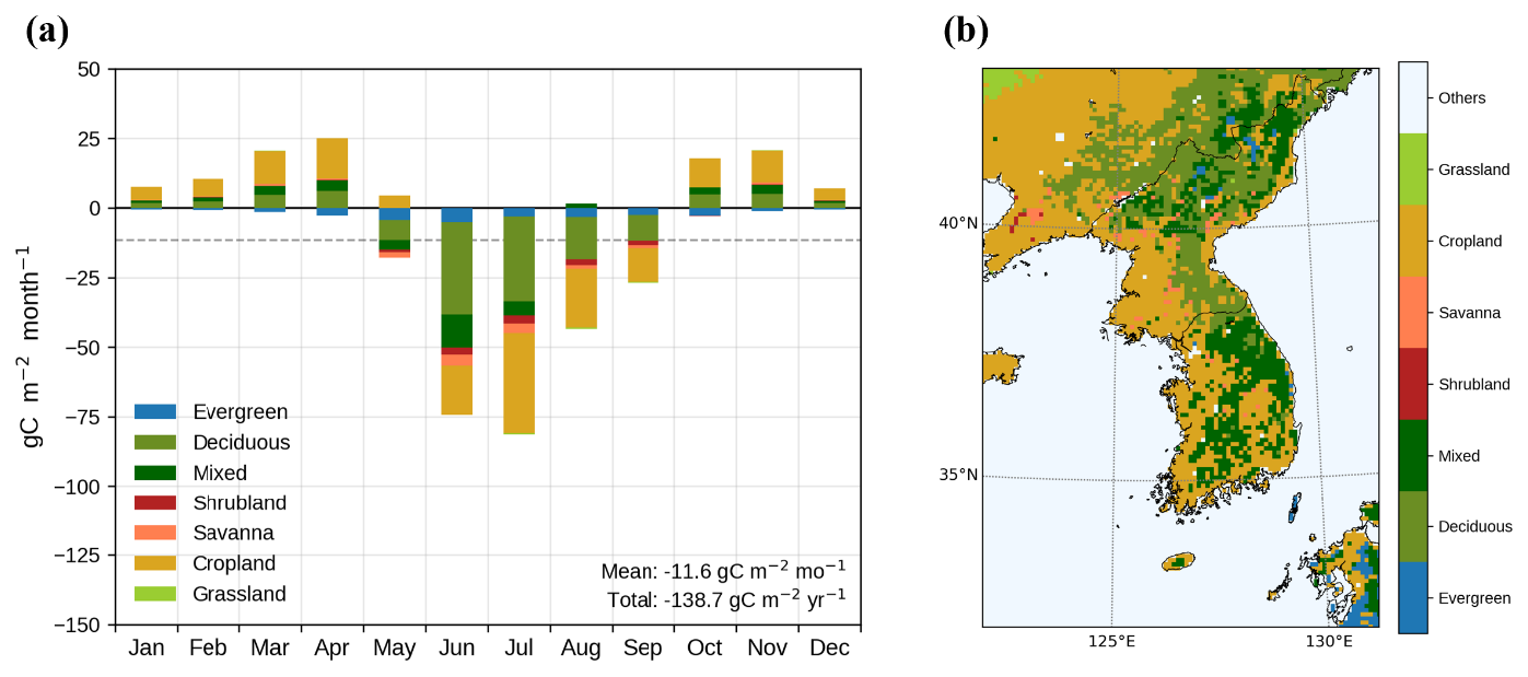
Figure 3 (a) Monthly net ecosystem exchange (NEE) contributions by vegetation class over the model domain in 2020. Bars show class totals (g C m⁻² month⁻¹), computed as spatial averages over grid cells of the corresponding vegetation type; negative values indicate net carbon uptake. (b) Spatial distribution of dominant vegetation classes used in WRF-Chem/VPRM; each grid cell is assigned the class with the largest vegetation fraction. Colors are consistent across panels.

6 Evaluation of the top-down estimates for 2020 case study

We now present a real-data demonstration to assess how the same cycling and analysis configuration performs under real observational constraints and inevitable model-data inconsistencies. We evaluated inversion results for 2020 using the WRF-Chem/DART system with full DA, in which both meteorological and GHG observations were assimilated. Each monthly run was initiated at 00:00 UTC on the last day of the preceding month, followed by a 24 h spin-up prior to the start of assimilation.

6.1 GHG concentrations at ground stations

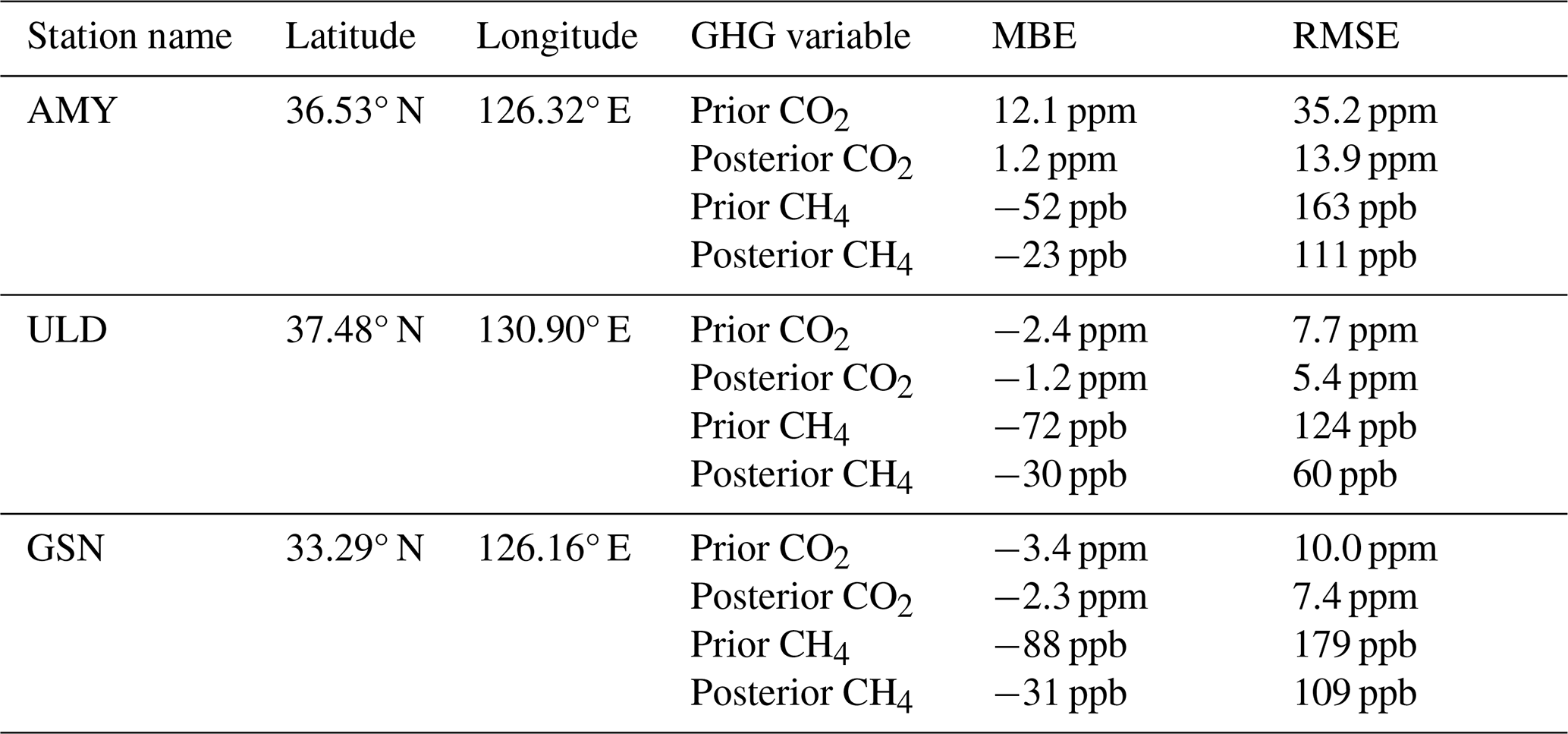
Monthly distributions of prior, posterior, and observed CO₂ and CH₄ concentrations at the three WMO/GAW surface stations are summarized with box plots for comparison of seasonal variability and site-to-site statistics (Fig. 4 and Table 1). Prior CO₂ concentrations overestimate the in situ observations at the AMY by about 12 ppm but underestimate at the remote stations (ULD and GSN) by 2–3 ppm. Prior CH₄ concentrations underestimate at all stations with annual mean biases of −52 to −88 ppb and particularly large discrepancies during the summer season. These biases are consistent with the expected influence of uncertainties in the prescribed EGG4 boundary fields. The top-down estimates of GHG concentrations show markedly improved agreement with observations relative to the prior, indicating the practical effectiveness of the EAKF system in reducing concentration-space mismatches. At the observation locations, the posterior estimates generally fall between the prior and the observations. Across all sites and both species, posterior estimates consistently reduce MBE (mean bias error) and RMSE (root mean square error) (Table 1). Mean bias of posterior surface CO₂ and CH₄ concentrations are in the ranges of 1–2 ppm and 20–30 ppb, respectively. The drivers of these improvements vary by site. The largest error reduction for CO₂ occurs at AMY (11 ppm), consistent with correction of a substantial prior positive concentration bias associated with nearby industrial sources and regional transport. In contrast, the largest improvement for CH₄ occurs at GSN (57 ppb), driven principally by the correction of the background bias and compensation for the latitudinal CH₄ gradient inherited from the CAMS EGG4 boundary conditions. Note that the DA system does not directly modify OH fields; rather, it adjusts CH₄ concentrations to match observations. Error reductions are most pronounced in summer, consistent with corrections to low-biased boundary inflow for CH₄ and to underrepresented seasonal regional fluxes (e.g., anthropogenic and biogeochemical contributions) when seasonal gradients are largest.

Notable differences are evident in the skewness of the monthly distributions of observed CO₂ and CH₄ concentrations across the sites. At AMY, both prior and posterior CO₂ and CH₄ exhibit strong positive skewness and high variability (elongated upper whiskers in Fig. 4a and d), depending on wind around nearby large point sources (i.e., power and industrial plants in the MWI). In contrast, GSN and ULD show more symmetric, compact distributions, suggesting weaker local source influence on these remote stations. All three stations exhibit a pronounced summertime dip in CH₄ concentration, especially in August. This feature is also evident in the EGG4 boundary fields used as lateral forcing (Fig. S11), suggesting that it primarily reflects large-scale seasonal background variability, potentially including enhanced summertime oxidative loss at hemispheric to continental scales, rather than regional chemical loss within the WRF-Chem domain.

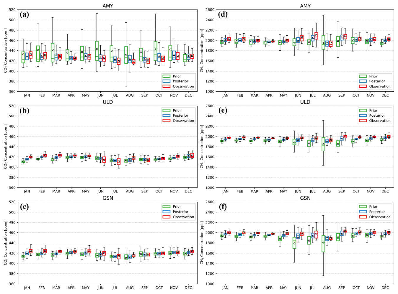
Figure 4 Monthly boxplots of CO₂ (a–c) and CH₄ (d–f) concentrations at AMY (a, d), ULD (b, e), and GSN (c, f) in 2020. Prior (green), posterior (blue), and observations (red) are shown for each site. Boxes denote the interquartile range (25th–75th percentiles); horizontal lines indicate medians. Symbols denote means (prior: circle; posterior: triangle; observation: square).

Table 1 Mean bias error (MBE) and root-mean-square error (RMSE) of the top-down estimates to the observations at AMY, ULD, and GSN in 2020. Statistics are computed from 6-hourly averages.

6.2 Validation against aircraft observations

To independently evaluate the performance of the inversion system, posterior CO₂ and CH₄ concentrations are compared with aircraft-based in situ observations collected over the Yellow Sea near the AMY station in 2020 using a Beechcraft King Air 350. The aircraft was equipped with a CRDS (G2401, Picarro Inc., USA) for measuring CO₂, CH₄, CO, and H₂O, at a sampling rate of 1.5 Hz. Sample air was dried upstream, and inlet ports were located near the front fuselage to minimize contamination. Typical operating altitudes reached 10 km with cruising speeds of 70–120 m s⁻¹, supporting both routine profiling and regional transport characterization. Ten vertical profile flights near the AMY were available in 2020 (not used in the data assimilation) (Fig. S9). After quality control, the profiles were aggregated into 1 km altitude bins (±500 m). Model fields were sampled along the flight track (time-matched and horizontally interpolated to the observation location) and averaged into the same altitude bins. For each bin, we computed mean observed concentrations and observational uncertainties (quadrature of sampling variability and reported measurement uncertainty) alongside the corresponding posterior values.

Figure 5 presents vertical profiles for CO₂ and CH₄ concentrations from both the inversion system and aircraft. Posterior CO₂ concentration is in good agreement with the observed profile with biases of 1–5 ppm even in the upper troposphere, whereas the posterior CH₄ concentration profile shows a systematic negative bias of 40–50 ppb from the boundary layer to the mid-troposphere. We speculate that this persistent CH₄ bias likely reflects a combination of residual boundary condition bias in the prescribed CAMS EGG4 inflow mole fraction and under-represented coastal CH₄ sources in prior data over the Yellow Sea. A controlled boundary-condition experiment supports the plausibility of this interpretation: imposing a CH₄ background bias of known size produces the weakest near-station CH₄ recovery, with a much smaller CO₂ response, consistent with the species-specific signature seen in the aircraft comparison (Supplement Sect. S1.3, Fig. S17). We present this as a consistency check rather than a unique attribution. It does not exclude possible contributions from under-represented coastal or inland CH₄ sources, residual transport error, or other boundary-condition uncertainties. The latter is consistent with the report that shallow shelves and coastal waters can be important CH₄ source regions (Lee et al., 2018; Weber et al., 2019). These results motivate further investigation of maritime CH₄ contributions in the regional prior/boundary treatment and highlight the value of additional observational constraints for improving CH₄ budgets over the Korean Peninsula.

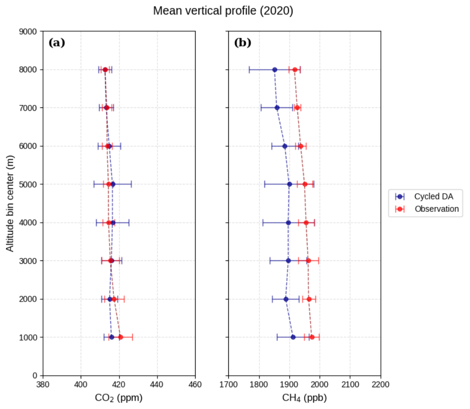
Figure 5 Mean vertical profiles of CO₂ and CH₄ from 10 CM-01 flights over South Korea in 2020. Profiles are aggregated into 1 km altitude bins (±500 m). Symbols and error bars show mean concentrations and associated uncertainties per bin: observations (red) and cycled DA (blue). Observation uncertainties combine measurement precision and sampling variability.

6.3 Uncertainty reduction in concentrations and fluxes

Figures 6 and 7 show the spatial distributions of ensemble spreads for CO₂ and CH₄ concentrations and the corresponding emission uncertainties, respectively, showing prior uncertainties (left panels) and uncertainty reductions after the DA (right panels). Unless noted, “uncertainty reduction” is defined as ($\mathrm{1}-{\mathit{\sigma }}_{\mathrm{post}}/{\mathit{\sigma }}_{\mathrm{prior}}$) × 100 % over grid cells where σ_post and σ_prior denote the posterior and prior ensemble spread, respectively. Domain-averaged concentration uncertainty over land decreases by 25 %–35 % for CO₂ and about 20 % for CH₄, with local reductions up to 50 % near the observation sites. Prior uncertainties in both concentrations and anthropogenic fluxes are elevated over strong source regions in SMA, large-scale power plants along the MWI, and the southeastern industrial areas (SCI and SEI) for CO₂. Elevated uncertainties for CH₄ are observed in landfills around the SMA, and in rice cultivation areas, as well as at livestock farms around CLA (compare Fig. 2 with Figs. 6 and 7). Posterior uncertainties in GHG concentrations decrease substantially within an influence radius of about 90 km (e-folding distance) from all the stations. CH₄ uncertainty reduction reaches up to 40 % around the station and has a larger relative decrease than CO₂. This is consistent with the negative bias in CH₄ concentration discussed above. We also note that uncertainty reductions over North Korea and China arise from weak cross-covariances at the range limit; these transboundary updates are not quantitatively interpreted in this study.

The spatial patterns of prior flux uncertainties closely resemble those for concentrations. Overall uncertainties for CO₂ emission decrease by about 7 % after the DA. CO₂ emission uncertainties decrease sharply within the influence radius of the AMY station along the western coasts, particularly for CO₂, where strong anthropogenic GHG sources are located (Fig. 7). Smaller reductions around ULD/GSN (< 5 %) reflect distance from major southeastern sources and prevailing winds. CH₄ emission uncertainties show a similar pattern with that of CO₂, except that the error reduction is relatively smaller than that of CO₂. Posterior flux uncertainty around AMY shows a relatively smaller reduction in CH₄ compared to CO₂, primarily because major CH₄ sources are located more easterly than those of CO₂. These patterns suggest qualitative priorities for future network expansion (e.g., enhanced CO₂ coverage in the southeastern industrial corridor and CH₄ coverage over central inland hotspots), while noting that a formal network optimization is beyond the scope of this paper. Because the maps are annual means, transient spatial structures at individual cycles are smoothed out; therefore, Figs. 6–9 should be interpreted as persistent features rather than cycle-to-cycle variability, with the strength of sub-national gradients remaining dependent on observational coverage.

The supplementary OSSE provides an idealized reference for this information-content limitation. Under perfect-model assumptions with a large prescribed prior-emission perturbation, the dense-network experiment (Figs. S20–S22) shows stronger national-scale CO₂ emission recovery than the corresponding three-site experiment, whereas the three-site case exhibits much weaker recovery under otherwise matched filter settings. This contrast indicates that the modest domain-mean flux-uncertainty reduction in the 2020 real-data case is consistent with limited observational information content, while also depending on the prescribed error statistics, localization, and prior-emission uncertainty. The companion error-source matrix supports this coverage interpretation: under the prescribed perturbations, transport-model, boundary-condition, and observation-error changes produce bounded changes in domain-mean recovery, and degrading observation precision has a limited effect on the domain-mean recovery under the tested configuration (Table S2). These results suggest that, for the present three-station setup, observational coverage is a dominant limitation on domain-wide recovery. Both the error-source matrix and the dense-network experiment are idealized diagnostics, not evidence of real-world flux accuracy or grid-scale resolvability.

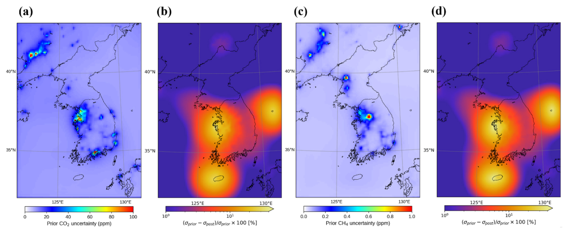
Figure 6 Annual prior concentration uncertainty (ensemble spread) (a, c) and its reduction after assimilation (b, d) for CO₂ (a, b) and CH₄ (c, d) in 2020.

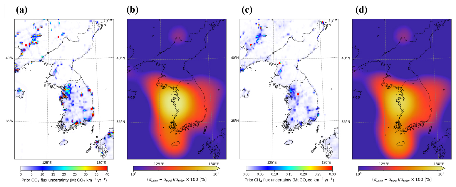
Figure 7 Annual prior flux uncertainty (a, c) and flux-uncertainty reduction (b, d) for CO₂ (a, b) and CH₄ (c, d) in 2020. Note that ocean-grid uncertainties are non-zero but appear small on the plotted scale because the prior spread is prescribed as a fractional perturbation and absolute oceanic flux magnitudes are much smaller than terrestrial sources.

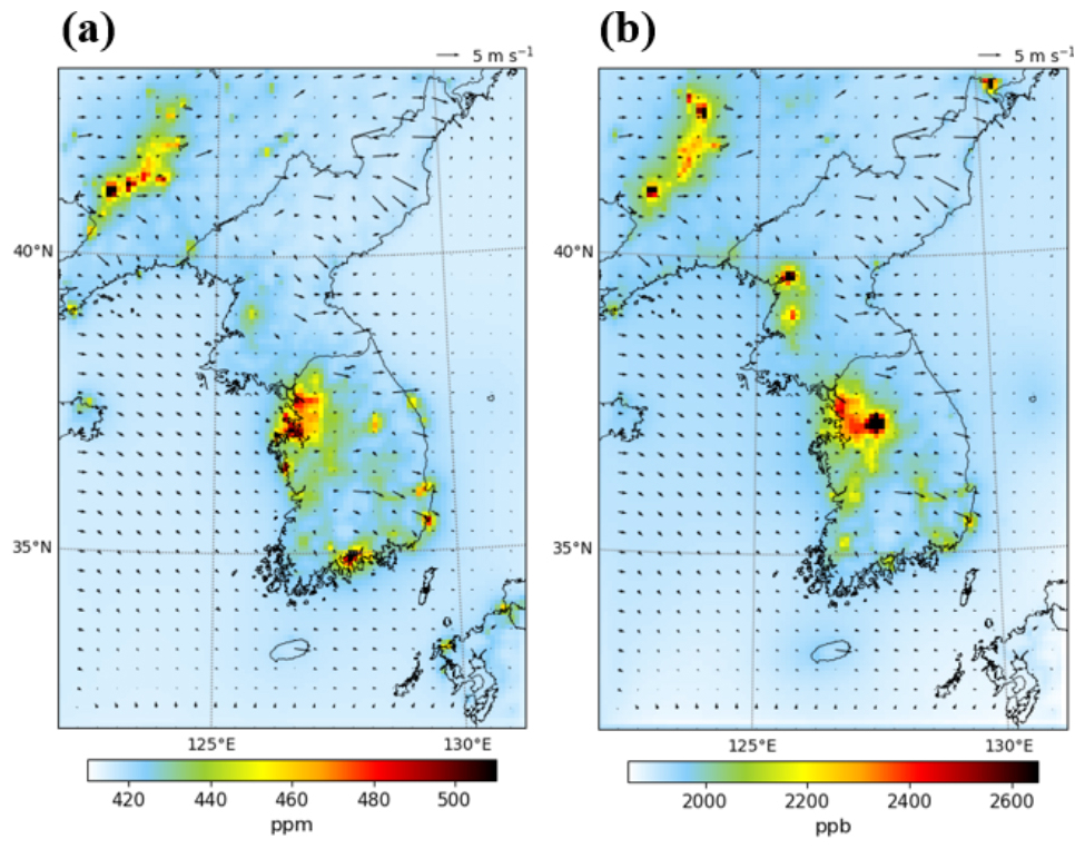
Figure 8 Annual mean surface posterior concentrations of CO₂ (a) and CH₄ (b) over the Korean Peninsula in 2020 from the WRF-Chem/DART inversion system. Wind vectors at 10 m illustrate prevailing flow conditions that shape annual concentration gradients.

6.4 Posterior fluxes and concentrations of CO₂ and CH₄

Figure 8 shows the spatial distribution of CO₂ and CH₄ concentrations from the inversion system. Posterior GHG concentrations capture large-scale gradients and regional enhancements induced by both long-range transport and upwind source regions. Elevated concentrations are clearly identified over key heavy industry and dense urban zones, specifically along the SMA, the west coast, and the southern industrial corridor (MWI, SCI, and SEI; Fig. 2b) for CO₂. In contrast, enhanced CH₄ concentrations are more closely associated with agricultural and waste-related source regions, including central–western Korea and the CLA region (Fig. 2c). When viewed alongside CAMS EGG4, both fields exhibit the broad synoptic structures, including persistent enhancements over the western Korean Peninsula and eastern China and the seasonal cycle of winter accumulation and summer dilution (Figs. S10–S13). This comparison is not used as an emission benchmark, because EGG4 does not solve for regional emissions in the same sense as the present inversion system; rather, it is used to illustrate differences in concentration-field representation between the coarse global boundary product and the high-resolution regional posterior. The structural differences between the two products primarily reflect differences in resolution: while EGG4 depicts spatially smoother concentration fields characteristic of its 0.75° global resolution, the 9 km posterior estimates represent sharper concentration gradients and more distinct source-region signatures over the SMA and MWI (Figs. 8 and S14a). Similarly, elevated CH₄ concentrations over the CLA are represented as more localized features in the posterior, whereas these appear as broader, more diffuse patterns in the global product (Fig. S14b). These features are consistent with previous satellite-based studies over Korea that documented fine-scale urban–industrial heterogeneity in CO₂ and CH₄ (Shim et al., 2019; Moon et al., 2024). The 9 km framework resolution is selected with future satellite-assimilation applications in view (e.g., TROPOMI CH₄ at ∼ 7 km footprint), where sub-grid representation error directly affects the forward operator. The present three-station in situ configuration does not by itself demonstrate grid-scale emission constraints at this resolution; however, retaining the 9 km transport framework facilitates future satellite-assimilation applications, provided that appropriate column observation operators, bias treatment, and representativeness-error specifications are implemented. Figure 9 summarizes the posterior anthropogenic flux fields and the spatial distribution of flux adjustments (posterior minus prior). The overall spatial patterns of posterior CO₂ and CH₄ emissions remain similar to the priors, retaining the major hotspots over the Korean Peninsula (Fig. 2b and c), as expected, given the current observing network and the use of covariance localization. Spatially-varying posterior adjustments are nonetheless produced to reduce concentration innovations at the observation sites. With the current observation configuration, these adjustments are best interpreted as regionally coherent corrections within the localization-supported influence region, while finer-scale structure remains strongly constrained by the prior and the assumed error statistics. Negative increments in CO₂ emissions are concentrated in densely populated and traffic-heavy regions (SMA and MWI) and positive increments are observed along the east coast and in the southeastern industrial corridor (i.e., SCI and SEI) (Fig. 9b). These patterns are broadly consistent with the signs of the station-based concentration biases (Table 1) and suggest that the positive bias at AMY tends to project onto nearby western source regions as flux reductions, whereas the negative biases at GSN and ULD can contribute to increased fluxes in the southern and eastern industrial regions through localized concentration–flux covariances. This behavior may also reflect sector-dependent structural uncertainties in the priors, given the strong contribution of heavy industry (steel, petrochemical, shipbuilding, and vehicle manufacturing) in SCI and SEI, relative to the more mixed urban/energy source in SMA/MWI. Positive increments for CH₄ emission are widespread across inland source regions associated with rice paddy, livestock facilities, landfills, and power-industry (Fig. 9d). Given the persistent negative CH₄ bias in the independent aircraft profiles (Sect. 6.2), we interpret these increases with caution because of the possibility for compensation for low-biased prescribed boundary mole fractions. At the same time, the spatial correspondence with known inland hotspots suggests that missing or underestimated sources in the prior may also contribute. The controlled OSSE matrix provides a scale for interpreting these sensitivities under prescribed conditions: transport-model, boundary-condition, and observation-error perturbations change the recovered domain emission by only a few percentage points of the prior inventory in the tested configuration, while the localization sweep produces somewhat larger changes (Table S2, Supplement Sect. S1.2–S1.3). These values should be interpreted as controlled diagnostic responses, not as universal bounds on real-world error. Further work with alternative boundary products and expanded observational constraints (e.g., additional in situ and upper-air measurements) is needed to extend this across the multiple sectors, times, and regions of a real application.

Figure 10 compares national-total anthropogenic CO₂ and CH₄ emissions for South Korea in 2020 from the posterior with multiple bottom-up inventories. For CO₂, the comparison encompasses Open-source Data Inventory for Anthropogenic CO₂ (ODIAC) (Oda et al., 2018), the Fossil Fuel Data Assimilation System (FFDAS) (Rayner et al., 2010), the Gridded Daily Fossil CO₂ Emissions Dataset (GRACED) (Dou et al., 2023), EDGAR, and the national total anthropogenic emissions (excluding the LULUCF sector) as reported in the Biennial Transparency Report of the Republic of Korea (ROK-BTR, hereafter). Because these products differ substantially in scope and construction (e.g., fossil-fuel-only versus IPCC-sector totals), proxy choice, point-source treatment, spatial disaggregation, native resolution, and sector attribution, we interpret the comparison as a consistency check under a harmonized scope (anthropogenic CO₂ excluding LULUCF) rather than as a validation target (Hutchins et al., 2017). Under the harmonized scope and spatial aggregation used here, EDGAR's national-total anthropogenic CO₂ is most consistent with the ROK-BTR estimate among the bottom-up datasets considered. EDGAR is the closest to ROK-BTR (4 % higher), whereas FFDAS, GRACED, and ODIAC show larger deviations, ranging from about −31 % to +10 %. In 2020, our posterior CO₂ total is broadly consistent with ROK-BTR at the national scale (Fig. 10). In contrast, posterior CH₄ total shows weaker agreement with the available bottom-up estimates, consistent with the larger structural uncertainty in CH₄ source characterization and spatial allocation noted in previous studies (e.g., Moon et al., 2024).

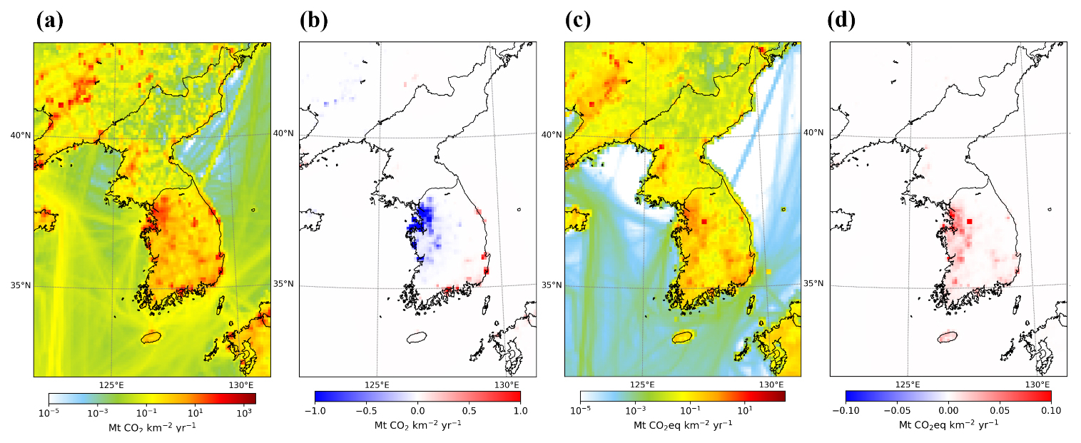
Figure 9 Annual-mean posterior surface fluxes (a, c) and assimilation increments (posterior minus prior) (b, d) for CO₂ (a, b) and CH₄ (c, d) from the WRF-Chem/DART system. Red (blue) shading indicates an increase (decrease) in the posterior relative to the prior.

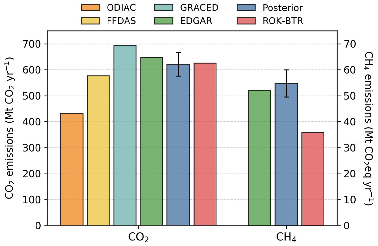
Figure 10 Annual total anthropogenic CO₂ and CH₄ emissions over South Korea in 2020 from multiple datasets. CO₂ comparisons include ODIAC, FFDAS, GRACED, EDGAR, ROK-BTR, and the posterior (six sources). CH₄ comparisons include EDGAR, ROK-BTR, and the posterior. Error bars denote posterior uncertainty. (FFDAS was scaled using the 2015–2020 gross emission growth rate from ROK-BTR because FFDAS is available only through 2015).

7 Summary and Conclusion

This study presents a high-resolution dual-species GHG (CO₂ and CH₄) inversion framework using the coupled WRF-Chem/DART system, which assimilates continuous high-precision in situ observations of GHG concentrations. The system provides transport-consistent and observation-constrained emission estimates and dynamically consistent temporal state updates through ensemble data assimilation. By updating both meteorological and tracer states within the cycling system, the framework maintains internally consistent transport–concentration relationships over complex terrain. The incorporation of continuous high-frequency in situ observations helps constrain near-surface gradients and the associated anthropogenic flux sensitivity.

This framework is designed to accommodate denser and more diverse observing systems (e.g., additional surface sites, tall towers, aircraft profiles, and satellite column retrievals) within the same data-assimilation framework; although extending to various types of observations may involve implementing the corresponding observation operators and specifying observation-error/representativeness settings (including bias treatment where applicable), together with network-dependent tuning (e.g., localization and observation error) as needed. A controlled OSSE matrix shows that, under prescribed transport-model, boundary-condition, and observation-error perturbations, the system produces bounded and interpretable emission responses rather than unbounded or unstable corrections. The complementary dense-network known-truth experiment indicates that expanded observational coverage substantially strengthens domain-wide CO₂ emission recovery in an idealized setting, while the real-case diagnostics of ensemble size and inflation configuration support the current 20-member, adaptive-inflation setup as a practical configuration rather than a uniquely optimized one.

The cycling dual-state EAKF framework provides an integrated treatment of background errors and filter stability within a joint state–parameter assimilation system for GHG concentrations and emissions. Because meteorology and 3-D tracer fields are advanced and analyzed within the same model, background-error covariances are represented in a flow-dependent manner by the evolving ensemble. The DART configuration provides an explicit, principled inflation framework to maintain physically plausible ensemble spread and to mitigate ensemble collapse during repeated cycling, offering a systematic handle on under-dispersion arising from unresolved transport/model errors and finite-ensemble sampling. These capabilities come with trade-offs. Running an ensemble is computationally more expensive than footprint-based calculations, and posterior updates depend on the fidelity of the underlying meteorological and sub-grid physical parameterizations that govern transport and mixing.

In the 2020 real-data application, the system reduces mismatches with observed CO₂ and CH₄ at all high-precision sites and yields posterior uncertainty reduction in both concentrations and emissions. The posterior surface biases are reduced to approximately 1–2 ppm for CO₂ and 20–30 ppb for CH₄ across the WMO/GAW sites in 2020, indicating improved consistency with local observations under the cycling configuration relative to the prescribed CAMS EGG4 IC/BC forcing. The posterior national CO₂ total (620 ± 45 Mt yr⁻¹) is consistent with the ROK-BTR estimate (624 Mt yr⁻¹) at the national scale. The posterior CH₄ total (54.7 ± 5.2 Mt CO₂eq yr⁻¹), however, exceeds the ROK-BTR estimate (35.5 Mt CO₂eq yr⁻¹) by 19.2 Mt CO₂eq yr⁻¹, which may reflect a combination of underestimated agricultural and waste-sector sources, residual boundary-condition bias, and structural uncertainty in CH₄ source characterization and spatial allocation. Regional adjustments relative to the prior are observed over densely populated, industrial, and agricultural areas for both species. Posterior increments suggest that prior CO₂ emissions may be overestimated over the Seoul Metropolitan Area and portions of the western coastal region, whereas CH₄ emissions may be underestimated over inland agricultural hotspots; CH₄ adjustments should be interpreted with caution, given the potential sensitivity to boundary-condition biases and maritime source representation. These results illustrate the potential value of top-down constraints for national-scale consistency checks and for guiding sub-national inventory evaluation. The current three-station configuration provides the strongest constraints within station footprints and should therefore be interpreted as a first operationally relevant regional demonstration, not as a claim of grid-scale emission resolvability. Broader observing-system configurations, including additional surface stations, upper-air measurements, and satellite column retrievals with appropriate bias and representativeness-error treatment, remain the primary pathway for improving domain-wide emission constraints. To our knowledge, this study provides the first fully documented regional WRF-Chem/DART workflow for simultaneous CO₂ and CH₄ estimation within a cycling dual-state configuration at kilometer-scale resolution, combining in situ GHG assimilation with meteorological data assimilation. Overall, this high-resolution dual-species WRF-Chem/DART inversion framework leveraging surface heterogeneity-aware parameterizations provides a reproducible basis for spatially explicit emission analyses that can support future policy applications, operational monitoring development, and MMRV-oriented evaluation at national and sub-national scales.