SPIN (v1.0): A spontaneous synthetic tropical cyclone model empowered by NeuralGCM for hazard assessment

A hybrid framework for simulating SPontaneous synthetic tropical cyclones (TCs) with realistic INtensity, hereafter SPIN, is developed for TC risk assessment. Unlike earlier statistical synthetic-TC models, SPIN retains intra-month variability and provides the ambient environment for each storm. The SPIN model leverages a Neural General Circulation Model (NeuralGCM) to simulate spontaneously generated TC tracks, and then couples a dynamical TC intensity model to estimate their intensity evolution based on the large-scale environment. It reproduces key features of observed TC climatology, including interannual variability, seasonal cycle, genesis and track patterns, lifetime-maximum intensity, regional landfall-intensity return periods and inter-genesis intervals. It also improves the representation of interannual TC variability in basins where ENSO-related influences are spatially mixed. Beyond individual TC events, the model demonstrates improved skill in representing multiple tropical cyclone events (MTCEs), capturing their year-to-year variability and cluster size. SPIN advances TC risk assessment by enabling compound TC hazards, such as MTCEs and beyond, to be assessed as dynamically organized events rather than statistical co-occurrences alone.

1 Introduction

Tropical cyclones (TCs) are among the most destructive hazards in coastal regions. On average, about 90 TCs form worldwide each year (Emanuel, 2006; Zhou and Lin, 2024), affecting 20.4 million people annually and causing mean direct economic losses of USD 51.5 billion over the past decade (Krichene et al., 2023). Beyond the impacts of individual storms, back-to-back TCs (Fu et al., 2025; Xi et al., 2023; Xi and Lin, 2021) can lead to especially severe impact, as communities may not recover from one event before the next occurs (Zscheischler et al., 2018). These societal consequences underscore the importance of assessing not only the risks of individual TCs but also those arising from their clustering.

The high risks associated with TCs have motivated the development of TC hazard downscaling frameworks. Here, “downscaling” denotes approaches that generate event sets large enough for risk assessment, rather than the spatial refinement of gridded meteorological fields. Over recent decades, two major approaches have been used for TC hazard downscaling: statistical and dynamical downscaling. Statistical downscaling models efficiently generate large ensembles of synthetic TCs from large-scale environmental conditions without requiring spatially explicit high-resolution wind fields, enabling estimates of extreme-event likelihoods at low computational cost. Statistical approaches include resampling methods based purely on historical observations (Bloemendaal et al., 2020; Vickery et al., 2000). Although useful for present-day risk assessment, such models are limited in their ability to represent non-stationary climates because they do not explicitly account for changes in the large-scale environment. To address this limitation, environment-dependent synthetic TC models have been developed to allow TC activity to vary with changes in climate conditions. These models differ in how they represent genesis, track and intensity evolution. Examples include statistical–dynamical models such as CHAZ (Lee et al., 2018), PepC (Jing and Lin, 2020), and the models developed by Emanuel et al. (2008) and Lin et al. (2023).

These models have several constraints when applied to compound TC hazard assessment. First, because they are driven by monthly-mean environmental fields, they are not designed to resolve intra-month variability relevant to TC genesis. Second, synthetic TCs are treated as independent events. Third, they do not provide time-evolving ambient environmental fields associated with each storm. These limitations make it difficult for traditional statistical downscaling models to move beyond statistical co-occurrence and represent compound TC hazards as dynamically organized events. Multiple tropical cyclone events (MTCEs), where two or more TCs occur simultaneously within the same basin (Fu et al., 2023; Schenkel, 2016), highlight this challenge because they are often controlled by intra-month variability (Gao and Li, 2011; Ito and Yamauchi, 2026) and disturbances from preceding storms (Ritchie and Holland, 1999; Yoshida and Ishikawa, 2013). In addition, for synthetic TC models based on random seeding (Emanuel et al., 2008; Lin et al., 2023), seeds are placed randomly in space and time rather than being diagnosed from evolving circulation fields, which may weaken the representation of interannual variability in TC frequency.

By contrast, dynamical downscaling explicitly simulates TCs in numerical models, allowing storm evolution to be embedded within an evolving environment. However, even the high-resolution models with grid spacing of 4–25 km still have difficulty in representing the most intense TCs (Buonomo et al., 2024; Davis, 2018; Judt et al., 2021). More importantly, they remain prohibitively expensive to run over sufficiently long periods to generate the large samples needed for robust TC risk assessment.

Recent advances in artificial intelligence (AI) weather forecast and climate models (Bi et al., 2023; Bodnar et al., 2025; Kochkov et al., 2024; Price et al., 2025) have made it possible to simulate synthetic TCs rapidly within evolving environmental fields. Building on this progress, Jing et al. (2024) developed a TC downscaling model based on a data-driven approach that accounts for two-way storm–environment interactions throughout the storm life cycle. Nonetheless, this approach still requires manually seeded vortices rather than permitting spontaneous genesis from environmental fields. In addition, as with numerical models, TCs directly extracted from AI-simulated outputs still tend to underestimate intensity, since the models are trained on ERA5 reanalysis data whose resolution cannot adequately resolve TC structure (Jing et al., 2024). In short, there remains a gap for models that can efficiently generate large ensembles of synthetic TCs that emerge spontaneously from evolving environmental fields while achieving realistic intensities and representing intra-month processes.

Rather than functioning like most AI weather forecast models, the Neural General Circulation Model (NeuralGCM) (Kochkov et al., 2024) offers sufficient stability for long-term climate simulations by preserving a GCM-like numerical solver for large-scale dynamics while replacing small-scale parameterization schemes with a neural network. It provides hourly large-scale environmental fields and reproduces key climate diagnostics with considerable skill, including realistic TC frequency and trajectories. Recent studies have further demonstrated NeuralGCM's ability in predicting seasonal TC activity under simplified boundary conditions (Zhang et al., 2025), long-term heatwave projections (Duan et al., 2025), the spectra of large-scale tropical waves (Baxter et al., 2025), and MJO teleconnections (Peings et al., 2026). Broader evaluations also show its skill in simulating extratropical cyclones, interannual teleconnection responses, and large-scale responses to out-of-distribution uniform-warming forcings, comparable to physics-based Earth system models (Chen et al., 2026). These features suggest that NeuralGCM provides a suitable basis for developing a synthetic TC downscaling framework.

In this study, we propose a hybrid framework that functions as a synthetic TC downscaling model, termed SPIN (a SPontaneous synthetic tropical cyclone model with INtensity fidelity). The model employs a two-step process: first, it leverages NeuralGCM (Kochkov et al., 2024) to simulate ensembles of spontaneously generated TC tracks; then, it couples these tracks with the FAST TC intensity simulator (Emanuel, 2017; Lin et al., 2023) to compute realistic intensities based on the large-scale environment. Compared with traditional statistical synthetic TC models, SPIN provides a more physically consistent representation of synthetic TCs and their ambient environment by generating storms that emerge from evolving environmental fields and by explicitly representing intra-month processes, while remaining substantially more computationally efficient than dynamical downscaling. This makes SPIN particularly well suited for studying compound TC hazards such as MTCEs.

This paper is organized as follows. Section 2 describes the data used for model development along with the model components and evaluation methods. Section 3 evaluates SPIN simulated climatological characteristics of TCs and MTCEs against observations. Section 4 compares observed and simulated return periods at different regions of the globe. Section 5 provides a summary and discussion.

2 Materials and methods

2.1 Observational and reanalysis data

The ERA5 reanalysis data (Hersbach et al., 2020) from 1979 to 2022 at 0.25°×0.25° resolution are used to initialize and force the NeuralGCM component of SPIN (see Sect. 2.2). The initialization fields include wind, geopotential, temperature, specific humidity, and specific cloud ice and liquid water content on pressure levels, while the forcing consists of sea surface temperature (SST) and sea ice concentration (SIC) at the surface level. The simulated TCs are evaluated at both global and basin scales. We adopt a similar basin classification as Lin et al. (2023), dividing the global ocean into seven basins where TCs are prevalent: the Western Pacific (WP), Eastern Pacific (EP), Northern Atlantic (NA), Northern Indian Ocean (NI), Southern Indian Ocean (SI), Southern Pacific (SP), and the Australian Basin (AU). The boundaries of each basin are illustrated in Fig. S1 in the Supplement. For model evaluation, we use the USA archive from the International Best Track Archive for Climate Stewardship (IBTrACS) (Knapp et al., 2010), which provides 3-hourly latitude and longitude positions as well as maximum sustained wind speeds for each storm.

2.2 Model components

The SPIN model follows a two-step approach (Fig. 1). First, it leverages NeuralGCM (Kochkov et al., 2024) to simulate ensembles of spontaneously generated TC tracks. Then, FAST intensity model (Emanuel, 2017; Lin et al., 2023) is coupled to each track to compute realistic intensities based on the large-scale environment. In this way, SPIN generates large samples of TCs that emerge from the simulated environment.

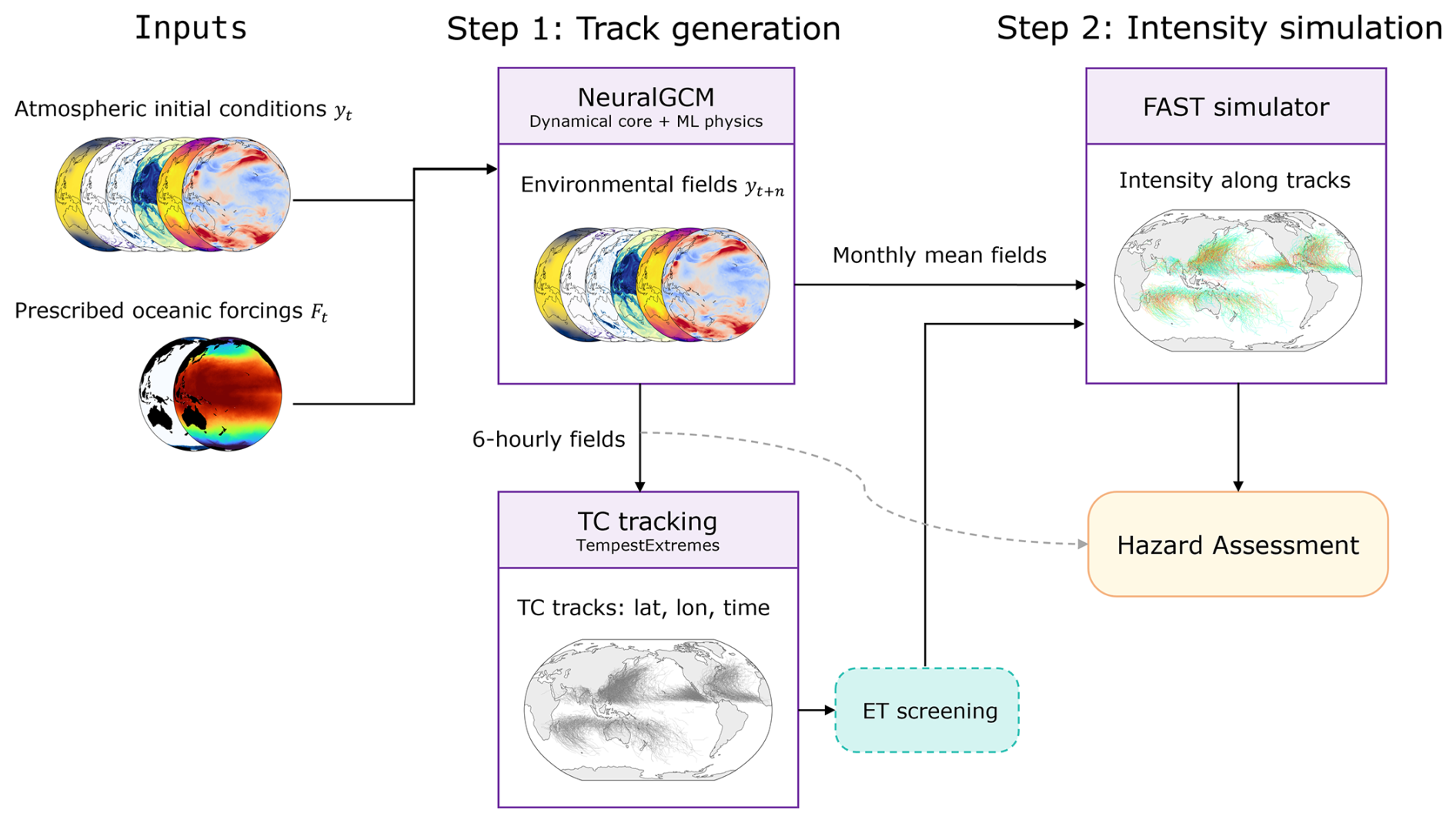
Figure 1 Workflow of the two-step SPIN modelling framework. In Step 1, atmospheric initial conditions y_t and prescribed oceanic forcings F_t are provided to NeuralGCM to generate environmental fields. The simulated 6-hourly environmental fields are used to detect and track TCs with TempestExtremes. Extratropical transition (ET) screening is then applied to the simulated tracks. In Step 2, the generated tracks and simulated monthly-mean environmental fields are passed to the FAST intensity simulator to estimate TC intensity along each track. The synthetic tracks and their ambient environments can then be used for hazard assessment.

2.2.1 Simulation of environmental fields

NeuralGCM is a hybrid physics-machine learning atmospheric model (Kochkov et al., 2024) that preserves a GCM-like numerical solver for large-scale dynamics, while replacing small-scale parameterization schemes with a neural network. It offers orders-of-magnitude computational savings over conventional GCMs and is sufficiently stable for long-term climate simulations. It has been shown to reproduce key climate diagnostics with considerable skill, and demonstrates promising performance in simulating realistic TC activity in tests for the year 2020 (Kochkov et al., 2024).

We use the pre-trained 1.4° deterministic version of NeuralGCM to simulate the environmental fields from which TC tracks are extracted. The 1.4° version is about ten times faster in inference than the 0.7° version and has been shown in previous studies to reasonably reproduce trajectories and counts of TCs (Kochkov et al., 2024; Zhang et al., 2025). For each target year from 1980 to 2022, we initialize a 14-member NeuralGCM ensemble simulation. The ensemble is generated using lagged initial conditions, with members initialized at 6 h intervals in mid-October of the preceding year and integrated continuously through December of the target year. For example, the simulations used for the 1980 analysis are initialized in mid-October 1979 and integrated through December 1980. The preceding October–December period is treated as spin-up, and the January–December period of the target year is used for TC tracking and subsequent analysis. All initial and lower-boundary fields are derived from ERA5 (see Sect. 2.1). The initial atmospheric states include wind, geopotential, temperature, specific humidity, and specific cloud ice and liquid water content on pressure levels. Monthly mean SST and SIC fields are linearly interpolated to 12-hourly resolution and prescribed as lower-boundary conditions throughout the simulations.

Following the NeuralGCM documentation (https://neuralgcm.readthedocs.io/en/latest/checkpoint_modifications.html, last access: 5 August 2026), we fix the global-mean log surface pressure to reduce long-term model drift and enhance numerical stability. Although this adjustment substantially improved the stability of the rollouts, numerical instability still occurs in approximately 1.75 % of simulated member months, defined by non-meteorological outliers followed by missing values across the domain at later output steps. To maintain a consistent ensemble size across target years, we generate three additional backup members using the same mid-October initialization protocol but independent initialization times. For each target year, unstable original members are removed before TC detection and replaced by full-year simulations from backup members for the same target year. Backup members are considered in a fixed order. For each target year, the first backup member-year that is both stable and not previously assigned within that target year is used for replacement. Backup member-years that have already been used within the same target year, or are themselves unstable, are skipped.

2.2.2 Tracking of TCs

We apply the TempestExtremes method (Ullrich et al., 2021) to track TCs from the simulated environmental fields, using geopotential and vorticity as primary criteria, and without imposing any minimum wind speed thresholds. In this study, most parameter settings in TempestExtremes are similar with those in Kochkov et al. (2024), who ensures that the global frequency of identified TCs matches the counts obtained from the 0.25°×0.25° ERA5 reanalysis data. We further fine-tune parameters separately for each basin, aiming to align the simulated historical annual average number of tracks and storm lifetimes with those reported in the IBTrACS. After track extraction, tracks whose points are located entirely over land are removed. A total of 14 ensemble members, each simulated for 43 years, produces approximately 52 000 tracks globally. The ensemble mean number of extracted TCs in each basin agrees well with the observations, without any additional bias correction (Fig. S2).

2.2.3 Intensity model

TC intensities along the modeled tracks are simulated with the FAST intensity model, originally proposed by Emanuel (2017) and Emanuel and Zhang (2017), and later extended to the global scale by Lin et al. (2023). FAST is a physically based and computationally efficient model that simulates the maximum sustained wind speed by solving two coupled ordinary differential equations. This model has been successfully used in probabilistic TC forecasting (Lin et al., 2020) and in physics-based statistical downscaling frameworks (Lin et al., 2023).

In the Lin et al. (2023; hereafter JL23) framework, only tracks that reach the intensity threshold of 18 m s⁻¹ within 48 h are retained, while others are discarded. In our approach, we retain all extracted tracks to maintain consistency with the observed track count. For tracks that do not reach 18 m s⁻¹ within 48 h, we apply a bias correction at the 48 h point and all subsequent times by adding a random constant offset, so that the intensity of 48 h is at or slightly above 18 m s⁻¹, following the protocol of Lin et al. (2023). All model parameters are adopted from Lin et al. (2023), except for the surface enthalpy coefficient (C_k). We use C_k=1.05 as the default setting for all SPIN results presented in this manuscript. This value is slightly smaller than the C_k=1.2 used in JL23 default settings, as larger values produced an overly heavy upper tail in the simulated LMI distribution under the 6-hourly forced SPIN configuration. No basin- or region-specific tuning is applied. However, this value is not intended to be an optimal calibration for every basin or regional intensity distribution. As noted in the JL23 documentation, model parameters are provided through the namelist for tuning. Users may therefore explore parameter space for application-specific regional hazard assessments. Because the FAST equations use a random draw to initialize the maximum azimuthal wind speed, the intensity simulation is not deterministic for a given track and environmental forcing. We therefore perform 10 simulations per track with different random draws, resulting in 10 intensity realizations for each ensemble member (equivalent to 6020-year of simulation in total). In our analysis, we define TC genesis as the first time the storm reaches 18 m s⁻¹, and dissipation as the last time it exceeds this threshold.

2.2.4 Extratropical transition screening module

For storms extending into the mid-latitudes, the FAST intensity model may continue to estimate intensity under a TC framework even after the storm has entered environments favourable for extratropical transition (ET) (Jones et al., 2003). This may lead to overestimated intensities and a positive bias in MTCE counts. We therefore implemented an optional ET-screening module that masks storm records after the onset of ET-like environmental conditions in analyses that depend on TC intensity.

ET involves structural changes in the storm core and would ideally be diagnosed using three-dimensional thermodynamic metrics such as cyclone phase space (CPS) diagnostics (Hart, 2003). However, applying CPS-based metrics to NeuralGCM-1.4° would require dedicated validation of the model's three-dimensional thermal phase of the storm. In particular, these metrics are sensitive to the resolution of the input data and lack universal thresholds for determining when ET occurs (Wood et al., 2023). Here, our objective is not to classify ET explicitly, but to limit retaining TC intensity after storms enter ET-favourable environments. We therefore use SST and latitude as simple environmental indicators. This choice is consistent with the physical understanding that ET is often associated with poleward motion into cooler SSTs (Evans et al., 2017), and with the statistical results of Bieli et al. (2020), which identified SST and latitude as important predictors of ET occurrence. Specifically, when both conditions are satisfied for two consecutive time steps, we truncate the storm starting from the first of those two time steps: (1) the area-averaged SST within a 2° radius of the storm center is ≤25.5 °C, and (2) the storm's latitude exceeds the basin-specific median ET latitude derived from IBTrACS. Sensitivity tests using SST thresholds of 25.0 and 26.0 °C and latitude thresholds shifted by ±2° show little influence on the reported results.

The screening is intended to limit the inclusion of records that are likely affected by extratropical transition, although the conclusions of this study are not sensitive to its application.

2.3 Model evaluation and benchmarks

2.3.1 Benchmark models

To assess the intensity component of SPIN, we benchmark against the physics-based statistical downscaling framework developed by JL23, which applies the FAST model to statistical synthetic tracks. The JL23 model is driven by monthly statistics of daily environmental winds at 250 and 850 hPa, together with monthly-mean temperature, relative humidity, and sea surface temperature.

For comparison of SPIN-simulated MTCE (see Sect. 2.5 for definition) metrics with statistical downscaling methods, we use two benchmarks: (1) the JL23 model, and (2) a monthly-uniform-sampled version of IBTrACS. Like most statistical downscaling models, the archived track output from JL23 provides storm year and month, together with the number of time steps since genesis, but not the specific calendar genesis date. We therefore assign genesis dates to JL23 tracks by uniformly sampling within each month, following previous studies (Xi et al., 2023), and use 1000 Monte Carlo simulations to quantify the associated uncertainty. The number of sampled tracks per basin in JL23 follows its own TC frequency. This uniform-sampling strategy assumes independent TC genesis and neglects storm-storm interactions. To circumvent the bias in TC genesis frequency in JL23, we also apply the same sampling approach to observed TCs from IBTrACS dataset. Comparing SPIN with these benchmarks, we test whether SPIN can more faithfully reproduce observed MTCE characteristics than a month-level uniform-sampling framework (both benchmarks).

2.3.2 Statistical metrics

To quantify SPIN performance compared to the benchmarks in simulating observed probability distributions of various TC-related metrics (e.g. LMI, TC inter-genesis intervals), we use two statistical measures: the Kullback-Leibler (KL) divergence and the area between the cumulative distribution functions (ACDFs) of the model and observations.

The KL divergence D_KL(O∥M) measures the difference between the probability distributions of model (M) and observations (O) for a given metric, reflecting the information loss when the model distribution is used to approximate the observations. It is particularly sensitive to regions where the model assigns low probability to events that are frequent in observations, and is therefore especially useful for evaluating differences in the tails of distributions. It is defined as:

$$\begin{array}{}\text{(1)}& D_{\mathrm{KL}}\left(O\parallel M\right)=\sum _i{P}_{\mathrm{O}}\left(i\right)\log \left({\displaystyle \frac{P_{\mathrm{O}}\left(i\right)}{P_{\mathrm{M}}\left(i\right)}}\right)\end{array}$$

where P_M(i) and P_O(i) denote the probability of the ith bin for the model and observations, respectively. The value of $D_{\mathrm{KL}}(O\parallel M)=\mathrm{0}$ indicates perfect agreement between the two distributions. Higher values indicate greater divergence.

The area between the cumulative distribution functions (ACDFs) of the model and observations quantifies the direction and magnitude of the distributional shift between the model and observations. It is calculated as:

$$\begin{array}{}\text{(2)}& \mathrm{ACDFs}={\int }_{-\mathrm{\infty }}^{+\mathrm{\infty }}\left[F_{\mathrm{model}}\left(x\right)-F_{\mathrm{obs}}\left(x\right)\right]\mathrm{d}x\end{array}$$

where F_model and F_obs are the CDFs of the model and observations, respectively. A positive (negative) value indicates that the model systematically underestimates (overestimates) the metric relative to observations.

2.4 Landfall locations

We discretize global coastline into evenly spaced milepost points using the 1:110 m Natural Earth shapefile (https://www.naturalearthdata.com/, last access: 5 August 2026). Mileposts are equally spaced along the coastline at approximately 1.4° arc-length intervals. For each storm track, the location that the TC first transits from ocean to land is identified as the landfall location. This point is then assigned to the nearest milepost based on geographic distance. The method is applied consistently to both observational and modelled tracks, enabling direct spatial comparison of landfall frequencies.

2.5 MTCE identification

MTCEs are defined as two or more TCs that simultaneously coexist within the same basin (Fu et al., 2023; Schenkel, 2016). In this study, the algorithm for identifying MTCE clusters is implemented as follows: (1) The genesis and dissipation times of each individual TC track are merged into a single timeline and sorted chronologically. (2) An MTCE cluster is defined to commence when the active TC count reaches or exceeds two, persists for as long as this condition is maintained, and terminates once the count falls below two.

For each identified MTCE cluster, the maximum value of the active TC count during its duration is defined as the peak concurrent TC count for that cluster.

2.6 Return period calculation

The return period RP(x) is defined as the inverse of the occurrence rate of a threshold event:

$$\begin{array}{}\text{(3)}& \mathrm{RP}\left(x\right)={\displaystyle \frac{\mathrm{1}}{r_x}}\end{array}$$

where x is the threshold applied to the metric of interest, and r_x is the occurrence rate of events satisfying that threshold. For landfall intensity I, the threshold event is I≥x. For MTCE intervals, the threshold event is Δt_MTCE≤x, where Δt_MTCE is the interval between successive MTCE onset times.

For discrete observational or model data, the return period is computed empirically as:

$$\begin{array}{}\text{(4)}& \mathrm{RP}\left(x\right)={\displaystyle \frac{T_{\mathrm{total}}}{N_x}}\end{array}$$

where T_total is the total sampling period (i.e., the total observation period or the sum of the total simulation period across all model realizations), and N_x is the number of events satisfying the threshold condition.

3 Model evaluation

This section evaluates the performance of SPIN in reproducing key TC characteristics. We first assess the large-scale environmental fields simulated by NeuralGCM, followed by annual frequency, seasonal cycle, patterns of TC genesis and track, and intensity statistics at the global scale. We then focus on MTCEs metrics in the WP and NA basins, where such events are most frequent (Fu et al., 2025).

3.1 Large-scale atmospheric environment

NeuralGCM captures the main climatological structures of the large-scale environments relevant to tropical cyclone activity. The ensemble mean reproduces the observed VWS pattern, including the subtropical maxima evident in ERA5, although regional biases remain (Fig. 2a–c). It also captures the broad vertical temperature structure, with warmer conditions in the lower troposphere and colder conditions aloft (Fig. S3), and reproduces the expected meridional contrast in Z300–Z500, an upper-level warm-core proxy used in TempestExtremes, with larger values in the tropics and smaller values toward higher latitudes (Fig. S4).

Upper-tropospheric temperature biases increase with rollout time (Fig. S3). Biases in Z300–Z500 and VWS vary seasonally, with Z300–Z500 tending to be higher than ERA5 during the early-to-peak TC season and lower during the late season, whereas VWS tends to be lower than ERA5 during the early-to-peak season and higher during the late season (Figs. S4 and S5). Monthly normalized root-mean-square errors (NRMSEs), normalized by the spatial standard deviation of the ERA5 reference fields, also generally increase with rollout time, indicating gradual bias growth during the simulations (Fig. 2d). Despite these biases, the broad agreement with ERA5 supports the use of NeuralGCM to simulate large-scale environmental fields relevant to TC hazards.

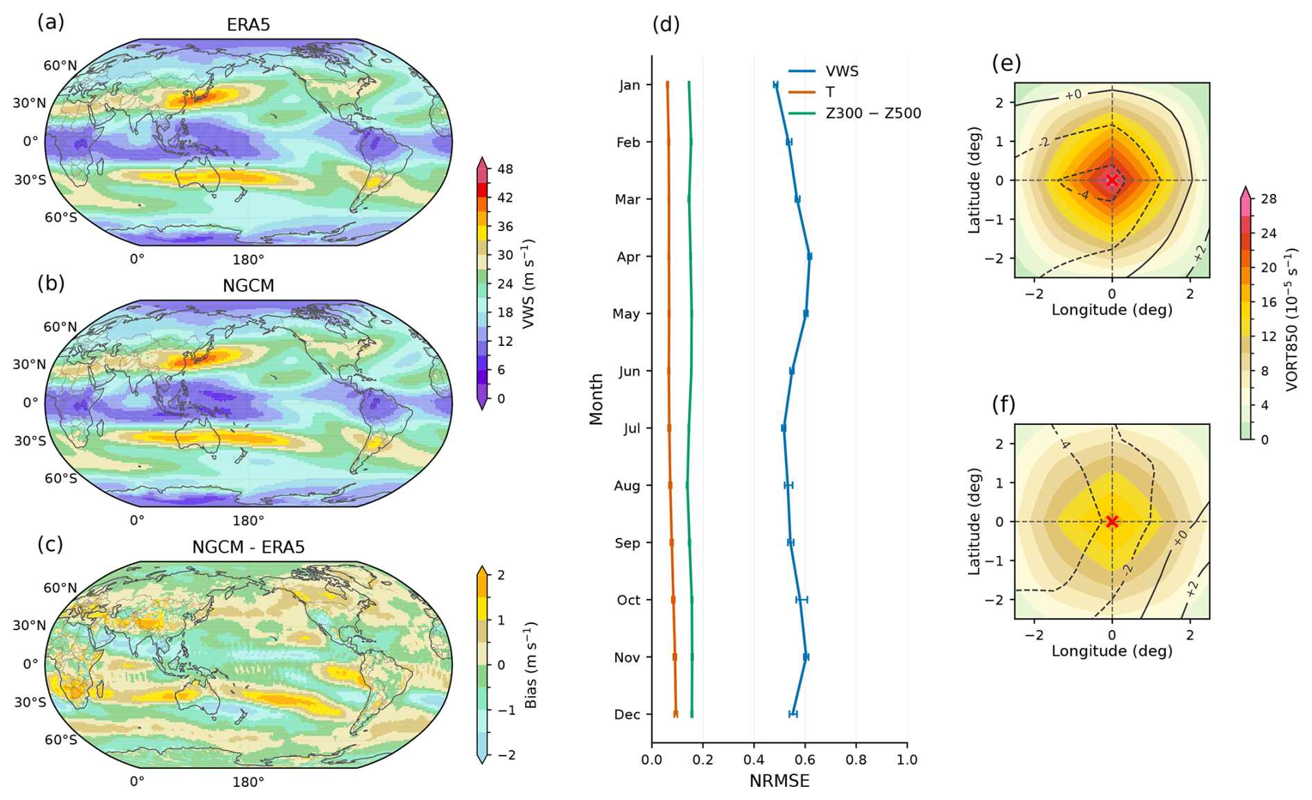
Figure 2 Evaluation of simulated atmospheric environmental fields. Panels show the 1980–2022 mean 200–850 hPa vertical wind shear (VWS; m s⁻¹) from (a) ERA5, (b) the NeuralGCM ensemble mean, and (c) their difference. Panel (d) shows monthly normalized root-mean-square errors (NRMSEs) between NeuralGCM and ERA5 for VWS, the meridional temperature profile (T; K), and the 300–500 hPa geopotential height difference (Z300–Z500; m² s⁻²), averaged over 1980–2022, with error bars indicating the 10th–90th percentile range across ensemble members. Panels (e) and (f) show storm-centred composites of the surrounding environment for FAST-simulated extreme TCs in the North Atlantic basin during 1980–2022. Composites are shown for the (e) top 10 % and (f) lowest 10 % of storms ranked by lifetime maximum intensity, evaluated at the time of lifetime maximum intensity. Shading shows 850 hPa relative vorticity (s⁻¹), and contours show surface pressure anomalies (hPa) relative to the mean pressure within a storm-centred 500–800 km annulus.

We next assess whether the FAST-derived intensity ranking is dynamically consistent with the corresponding NeuralGCM atmospheric fields. Using the NA basin as an example, the top 10 % of storms ranked by lifetime maximum intensity show stronger 850 hPa relative vorticity and surface pressure anomalies than the lowest 10 % (Fig. 2e, f). This correspondence indicates that the FAST-derived intensity ranking is qualitatively reflected in the NeuralGCM atmospheric fields.

3.2 Interannual variability and seasonal cycle

To evaluate the model's ability to represent interannual variability in TC activity, we calculated the correlation coefficients between basin-scale TC frequency in SPIN and observations over 1980–2022 (Fig. 3). Consistent with previous statistical downscaling models (Lee et al., 2018; Lin et al., 2023), SPIN performs best in the EP and NA basins (r=0.53 and r=0.47, respectively). We use January–December simulations here to maintain comparability with previous hazard-model evaluations (Lee et al., 2018; Lin et al., 2023). For application-oriented experiments, however, initializing closer to the target TC season can shorten the forecast lead time and reduces the accumulation of model drift. Consistent with this interpretation, April initialization simulations followed by evaluation over the Northern Hemisphere hurricane season yields higher basin-scale TC-frequency correlations (Fig. 4).

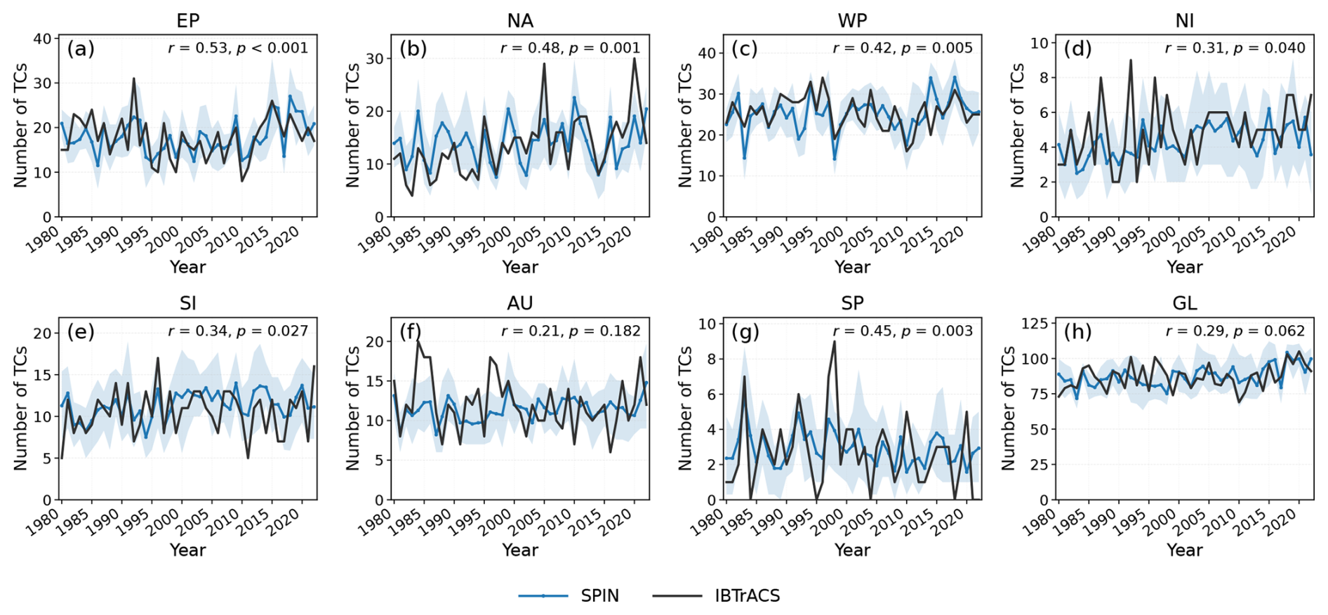
Figure 3 Interannual variability of TC frequency during 1980–2022. Panels show the (a) EP, (b) NA, (c) WP, (d) NI, (e) SI, (f) AU, (g) SP, and (h) GL basins. The blue line shows the ensemble mean of 14-member SPIN simulations initialized in mid-October at 6 h intervals, with shading indicating the 10th–90th percentile range, and observations are shown in black. Pearson correlation coefficients (r) with significance levels (p) are reported in the upper-right of each panel.

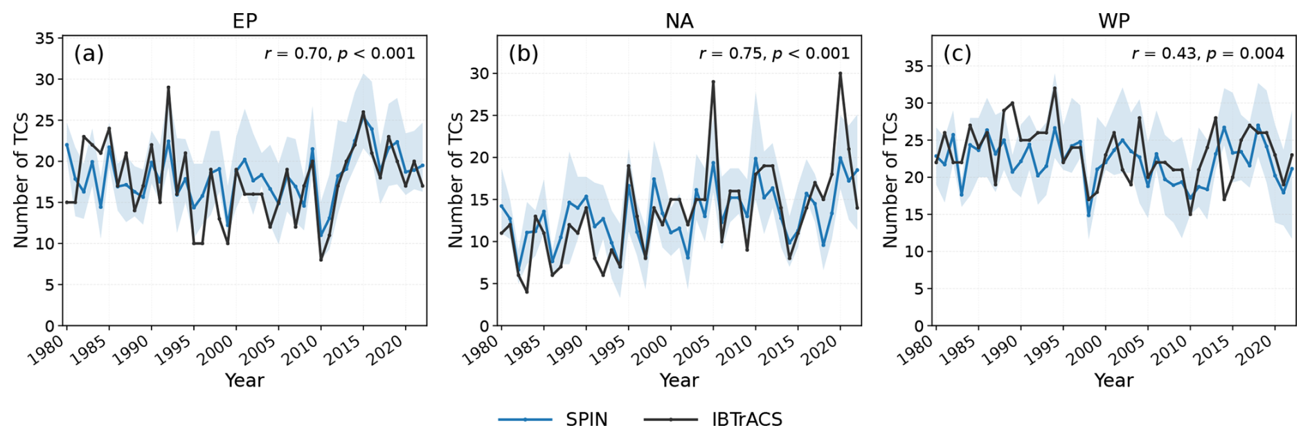
Figure 4 Interannual variability of TC frequency during May–December from 1980 to 2022 for the EP, NA, and WP basins. The blue line shows the ensemble mean of 14-member SPIN simulations initialized in early April at 6 h intervals, with shading indicating the 10th–90th percentile range. Observations are shown in black. Pearson correlation coefficients (r) with significance levels (p) are reported in the upper-right of each panel. Global-mean log surface pressure was not fixed in these simulations, as model drift is negligible over their integration timescale.

SPIN also shows markedly improved agreement with observations relative to JL23 in the WP, SP, and SI basins. Lin et al. (2023) suggested that lower predictability in these basins may reflect the mixed-sign influence of El Niño–Southern Oscillation (ENSO) on TC genesis across subregions (Fig. S6, Camargo et al., 2007; Lin et al., 2023), which can cause the basin-integrated interannual genesis signal to be averaged out. In contrast, SPIN better retains ENSO modulation in these basins, with ENSO conditioned TC frequency anomalies closer to IBTrACS than JL23 (Fig. S7). A possible reason is the difference in the treatment of seed disturbances. Previous diagnostic frameworks express TC genesis rates as the product of seed frequency and a transition probability controlled by the large-scale environment (Emanuel, 2022; Hsieh et al., 2020). JL23 uses random seeding (Emanuel et al., 2008; Lin et al., 2023), in which seeds are placed randomly in space and time and then allowed to evolve within the large-scale environment. Because this seed supply is not dynamically coupled to ENSO related circulation changes, it may artificially increase genesis probability in low-activity regions while decreasing it in high-activity regions. In contrast, SPIN diagnoses candidate storms from the evolving circulation fields generated by NeuralGCM. This allows SPIN to retain year-to-year changes in both environmental favorability and precursor disturbance supply. We regard this as a plausible mechanism rather than a definitive attribution. Overall, these results highlight the potential of SPIN to capture interannual variability in TC activities across most basins.

For the seasonal cycles of TC genesis (Fig. 5), SPIN reproduces the bimodal distribution in the NI basin and the unimodal patterns in other basins, with a slight tendency to overestimate TC counts from the early to peak season and underestimate them from the peak to late season. A similar bias was noted by Zhang et al. (2025, Supplement) that evaluates the performance of NeuralGCM. This seasonal bias is likely linked to the large-scale environmental biases in NeuralGCM. As shown in Sect. 3.1, NeuralGCM tends to predict lower VWS than ERA5 during the early-to-peak TC season, but higher VWS during the late season (Fig. S5). These biases favour TC genesis earlier in the season but suppress it later, consistent with the simulated seasonal genesis bias.

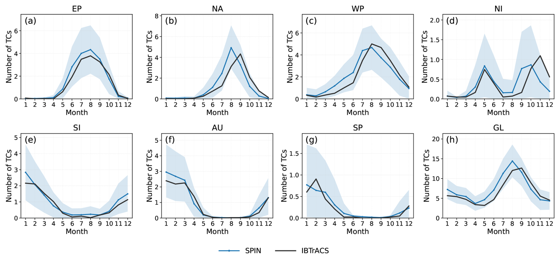
Figure 5 Seasonal cycle of TCs genesis averaged over 1980–2022. Panels show (a) EP, (b) NA, (c) WP, (d) NI, (e) SI, (f) AU, (g) SP, and (h) GL basins. The blue line shows the SPIN ensemble mean, with shading denoting the 10th–90th percentile range. Observations are shown in black. Only storms with lifetime maximum intensity exceeding 18 m s⁻¹ are included.

3.3 Genesis and track statistics

We first compare the spatial pattern of SPIN-simulated TC genesis patterns with observations from 1980–2022. 3°×3° grid boxes are used to calculate the genesis density (Fig. 6). Overall, the spatial pattern of simulated genesis events aligns well with historical observations, though some regional biases remain. For example, SPIN tends to underestimate genesis frequency in the Bay of Bengal, the South China Sea, the Philippine Sea, the northern part of the AU basin, the eastern part of the EP basin, the Gulf of Mexico, and the western part of the NA basin. In contrast, it tends to overestimate genesis in the southern parts of the Eastern Pacific and NA basins, as well as in the northern part of the WP basin. Several reasons may contribute to this bias. First, TC numbers are sensitive to the detection scheme; although we have fine-tuned the detection method to allow TC numbers to align with observations at the basin scale, subregional differences remain. Second, in SPIN, NeuralGCM is forced with monthly SST and SIC fields linearly interpolated to 12 h resolution. The interpolated forcing fields lack sub-monthly scale variability, which may also introduce bias. In addition, because genesis is defined as the first time the simulated surface wind of a TC exceeds 18 m s⁻¹, the bias in the intensity model may also influence the location of genesis events. Nevertheless, despite these biases, SPIN demonstrates skillful performance in reproducing the observed spatial distribution of TC genesis.

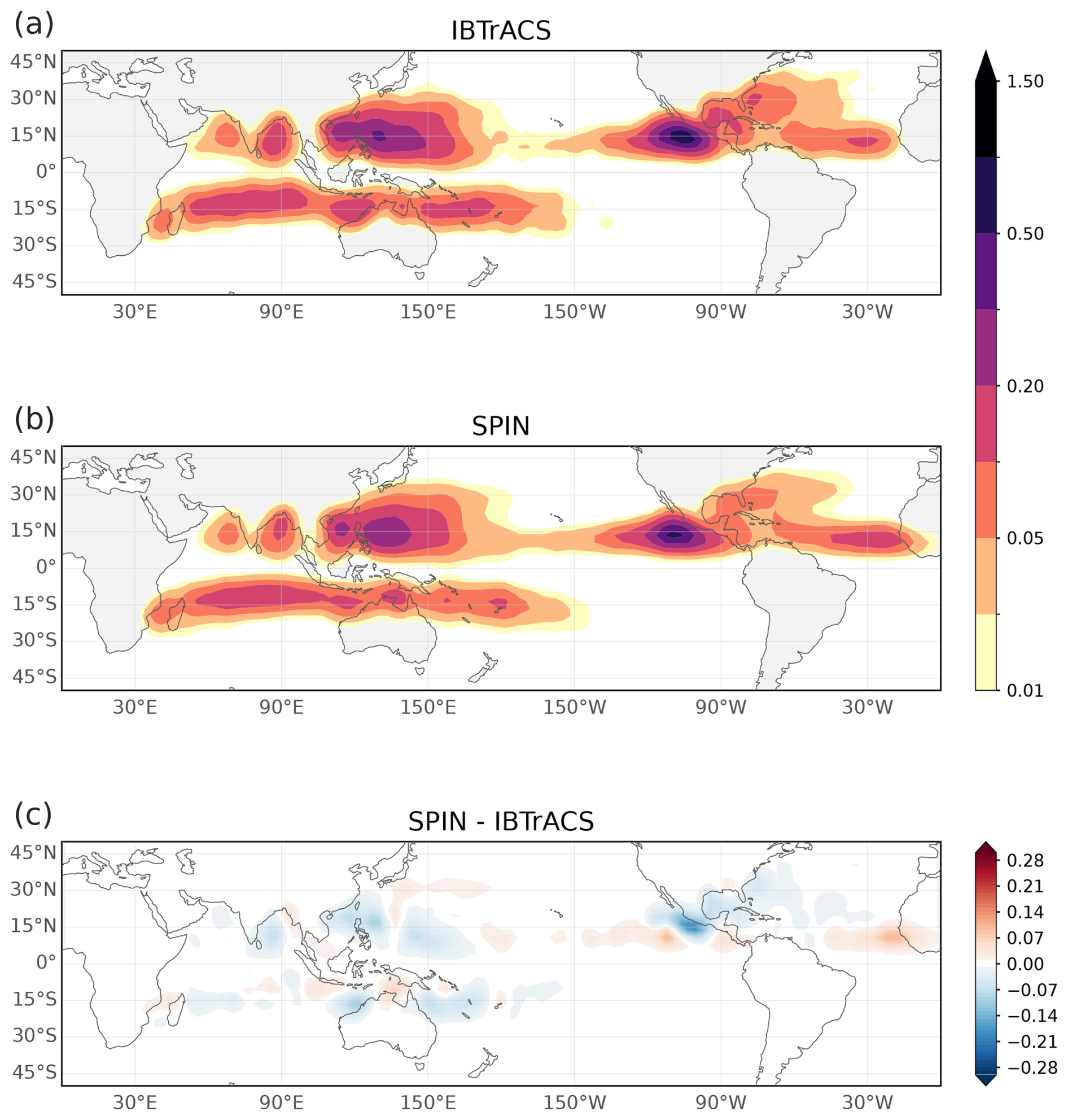
Figure 6 Tropical cyclones (TCs) genesis density per year on a 3°×3° grid with Gaussian smoothing averaged over 1980–2022. (a) IBTrACS, (b) ensemble-mean simulations from SPIN, and (c) their difference (b–a). Genesis is defined as the first occurrence time that a TC's maximum wind speed ≥18 m s⁻¹.

To assess how well SPIN captures TC translation characteristics, Fig. 7 compares the 6-hourly zonal and meridional displacements of simulated tracks with those from observations. SPIN tends to underestimate the magnitude of the displacement, suggesting that simulated biases in the steering flow (e.g., the subtropical high and trough structures) may appear overly smoothed (Duan et al., 2025). Such biases can in turn affect the recurvature latitude. Nevertheless, the overall simulation results show good agreement with observations.

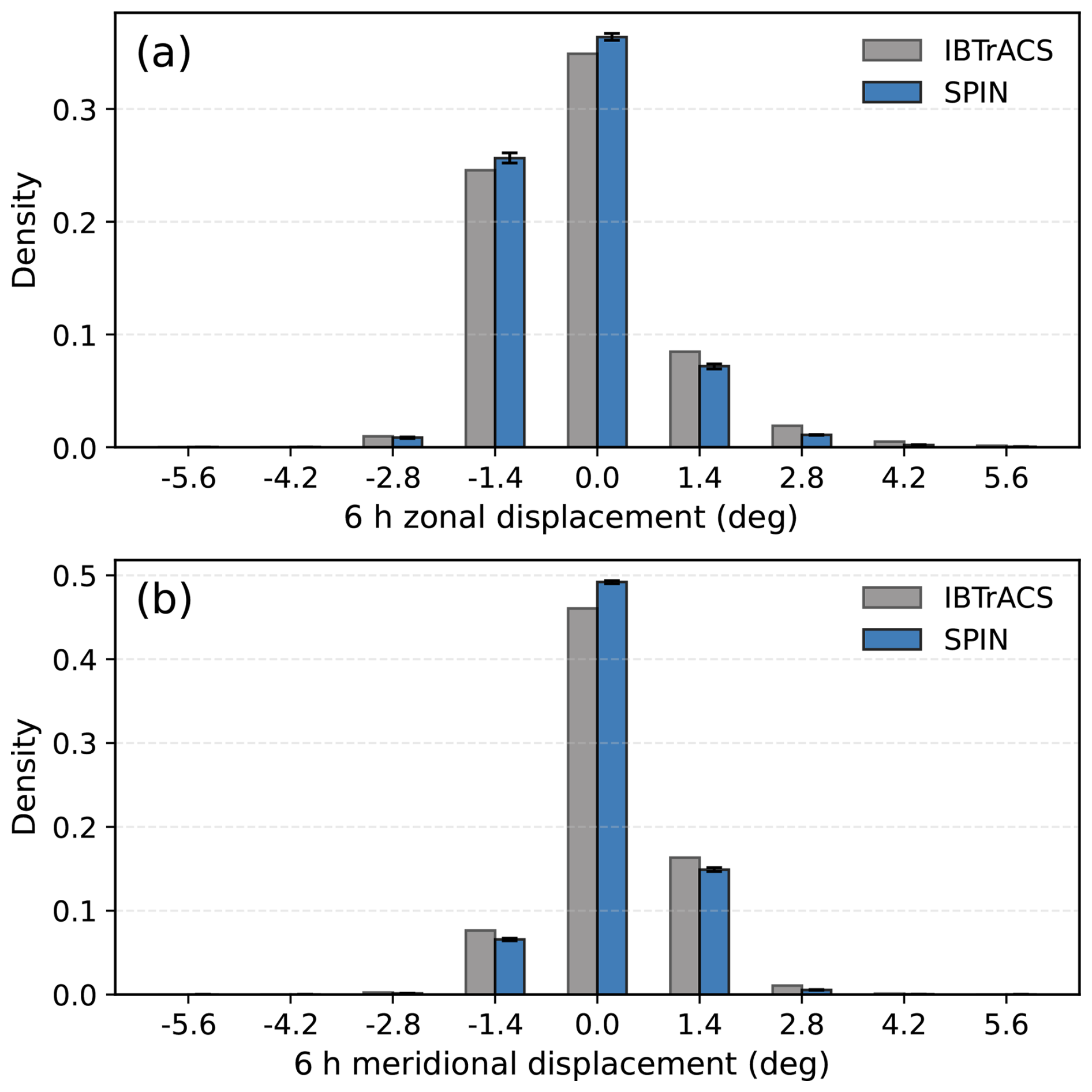
Figure 7 Comparison of 6 h TC displacement statistics between observations and the SPIN ensemble. (a) Zonal and (b) meridional displacements of TCs in IBTrACS (grey) and SPIN (ensemble mean, blue). Error bars indicate the 10 %–90 % ensemble spread for SPIN. Bins are defined at 1.4° intervals.

Next, we validate the annual track density simulated by SPIN. We calculate track density using 1°×1° grid boxes (Fig. 8). The spatial pattern of the bias of track density resembles that of genesis density, with SPIN underestimating density in the Bay of Bengal, southern part of WP basin, the northern part of the AU basin, and the northern part of the EP and NA basin. These biases in track density are therefore largely attributable to bias in simulated genesis locations. Differences in TC duration may also contribute to the bias in track density, with SPIN producing a mean global TC duration of 5.74 versus 4.85 d in the observation.

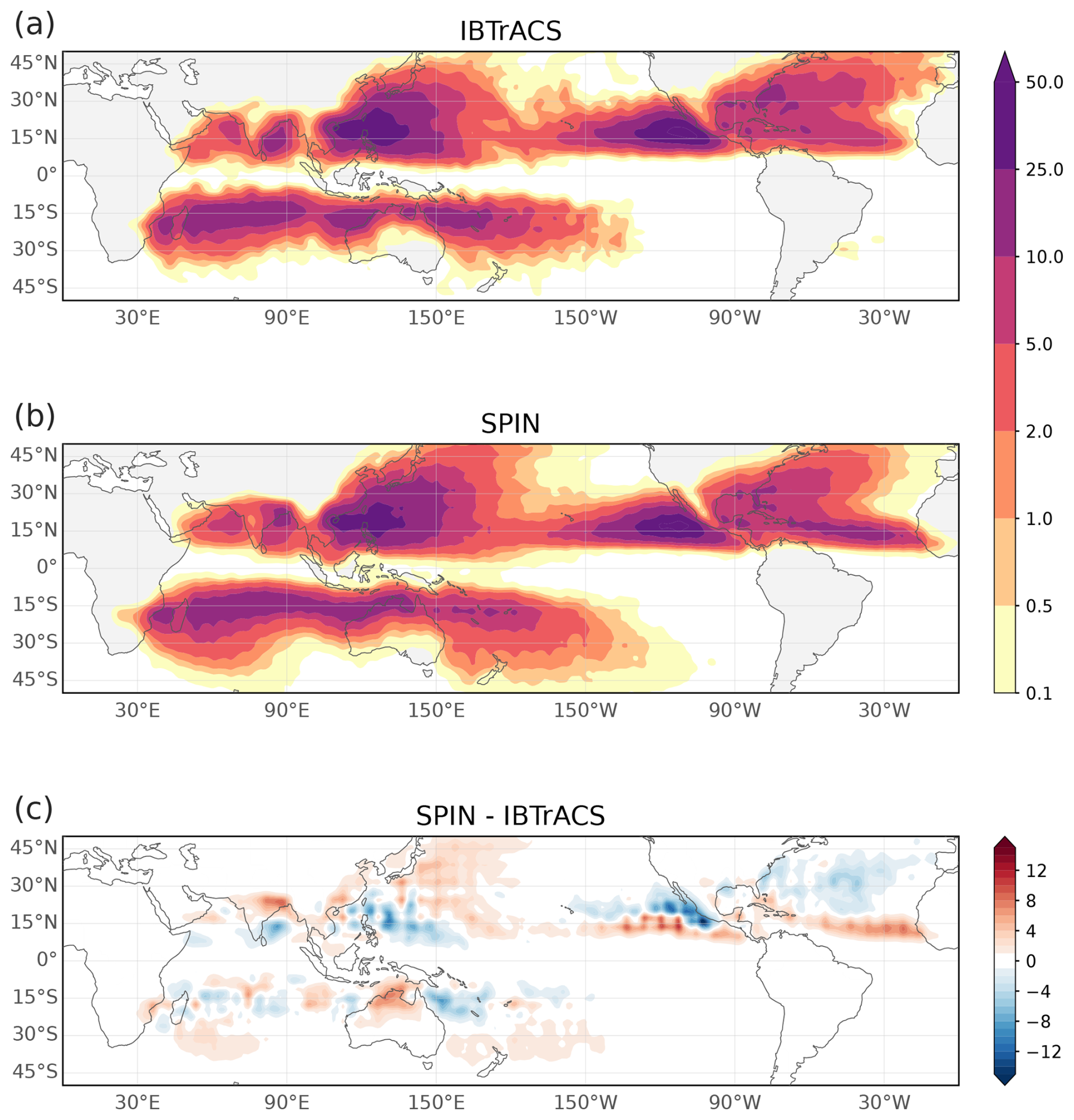
Figure 8 Annual 6-hourly TCs track density on a 1°×1° grid with Gaussian smoothing for 1980–2022. (a) IBTrACS, (b) ensemble-mean simulations from SPIN, and (c) their difference (b–a). Only storms reaching maximum wind ≥18 m s⁻¹ are included, with tracks evaluated from the first occurrence of that threshold.

3.4 Lifetime maximum intensity

We compare the SPIN-simulated lifetime maximum intensity (LMI) of TCs with observations at the global scale and in the basins with most TC-related economic losses, i.e., the NA and WP basins (Krichene et al., 2023) (Fig. 9). For comparison, we include the JL23-downscaled ERA5 experiment, hereafter JL-ERA5, which also uses the FAST intensity model (Emanuel, 2017). We further include a JL23-downscaled NeuralGCM experiment, hereafter JL-NGCM, to assess how biases in the NeuralGCM large-scale environment affect the simulated LMI distribution.

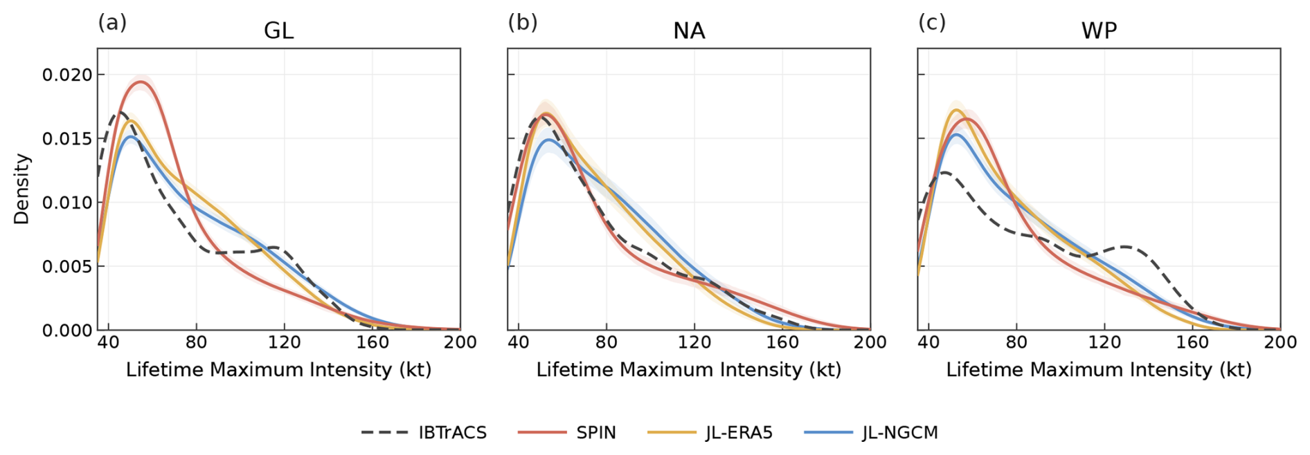
Figure 9 Distribution of LMI of TCs during 1980–2022. (a) shows the global distribution, (b) the NA basin, and (c) the WP basin distributions. Distributions are estimated using Gaussian kernel density fitting. Results of IBTrACS are shown as black dashed lines, SPIN simulations in red, JL-NGCM (using a single ensemble member) in blue, and JL-ERA5 in yellow. For JL-NGCM and JL-ERA5, downscaled events are randomly subsampled to match the number of observed events. For SPIN, shading denotes the 10th–90th percentile range across ensemble members; for the JL-downscaled results, shading denotes the 10th–90th percentile range from repeated subsampling to the observed sample size.

Both SPIN and JL23-downscaled models capture the main features of the observed LMI distributions, with most storms reaching weak-to-moderate intensities and progressively fewer storms reaching the highest intensities. This agreement is reflected in relatively small D_KL(O∥M) values, which range from 0.015 to 0.085 for SPIN, compared with 0.030 to 0.101 for JL-ERA5 and 0.029 to 0.048 for JL-NGCM (Table S1). Nevertheless, the agreement varies across basins. SPIN performs best in the NA basin, where the simulated distribution closely follows IBTrACS. In the GL and WP domains, the simulated distributions show a modest shift toward weaker-to-moderate intensities and a reduced frequency of some higher-intensity storms. A similar tendency is also evident in the JL23-based experiments, particularly in the WP basin.

These biases likely originated from the following model limitations. One common limitation is the underestimation of rapid intensification in the FAST intensity framework. The observed RI ratio ranges from 23.3 % to 33.2 % across the GL, NA and WP domains, whereas the simulated values are 6.0 %–11.1 % in SPIN, 8.1 %–11.6 % in JL-NGCM and 10.5 %–14.0 % in JL-ERA5 (Fig. S8). For SPIN, track-distribution biases may also contribute. In particular, excessive track occurrence at higher latitudes in the GL and WP domains may place more storms in environments less favourable for reaching high LMI (Figs. 8 and 9). The broad similarity between JL-ERA5 and JL-NGCM suggests that biases in the NeuralGCM large-scale environment are not the dominant source of the LMI bias, although they may still contribute. Overall, the remaining LMI biases appear to arise from a combination of limitations in the intensity model, biases in the track detection algorithm and residual environmental fields errors.

3.5 Landfall frequency

We next assess SPIN's ability to reproduce landfalling TC activity by comparing simulated landfall frequencies across major TC-affected regions (Fig. 10). The comparison shows SPIN has negligible bias relative to observations, particularly for Gulf–Atlantic Region, and China. In India, Australia, and Japan, spatial patterns of the bias in landfall frequency largely mirror those in track density. Also, due to the complex geometry of the coastline and the coarser spatial resolution of the modeled tracks, the first ocean-to-land crossing of a modeled track may not correspond to the actual landfall location, thereby leading to incorrect milepost assignments. Despite these biases, SPIN successfully reproduces the spatial pattern of landfall hotspots.

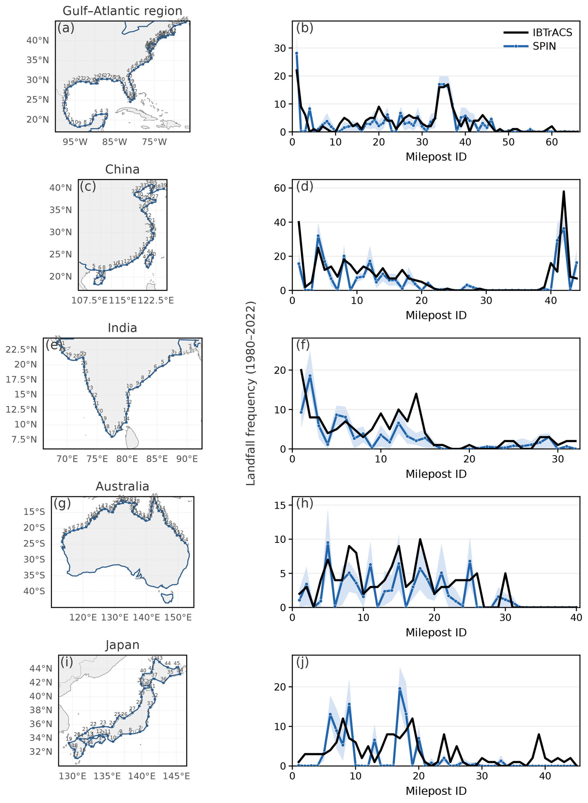
Figure 10 Landfall frequency of TCs along coastline mileposts during 1980–2022. Mileposts are equally spaced along the coastline at approximately 1.4° arc-length intervals for (a) Gulf–Atlantic Region, (c) China, (e) India, (g) Australia, and (i) Japan. The SPIN ensemble-mean landfall frequencies are shown in (b), (d), (f), (h), and (j) in blue, with shaded bands indicating the 10th–90th percentile range across ensemble members. Observations are shown in black.

3.6 Inter-genesis intervals

We assess whether SPIN realistically reproduces TC inter-genesis intervals in each basin (Fig. 11). Traditional statistical downscaling models, such as JL23, provide the month of TC genesis and the corresponding storm lifetime, but do not resolve intra-month variability needed to determine daily genesis time. As a result, previous studies of back-to-back TCs have derived event onset times by statistically sampling dates (Xi et al., 2023; Xi and Lin, 2021). This procedure assumes that individual TCs occur independently within the month and ignores intra-month processes that organize TC genesis.

Figure 11 Histogram of TC inter-genesis intervals from 1980–2022. Calculations are limited to the TC season in each year, defined as April–November for Northern Hemisphere basins (EP, NA, WP, NI; panels a, c, e, g) and from November to the following April for Southern Hemisphere basins (SI, AU, SP; panels b, d, f). Results from IBTrACS (black), IBTrACS with uniformly sampled dates (grey), the ensemble mean of SPIN simulations (red) are shown for comparison. Error bars denote the 10th–90th percentile range across ensemble members for SPIN and across 1000 Monte Carlo realizations for the uniform experiments.

We include IBTrACS with uniformly sampled genesis dates (hereafter IBTrACS-uniform) for comparison, providing a clean reference of TC inter-genesis interval distribution without the influence of biases from statistical downscaling models. SPIN exhibits lower D_KL(O∥M) values than IBTrACS-uniform in most basins, indicating a closer match to observations (0.012–0.069 for SPIN versus 0.019–0.182 for IBTrACS-uniform; Table S2). Additionally, IBTrACS-uniform tends to show a stronger left skew in its distribution, particularly within the 0–5 d bin, with ACDF values ranging from 0.25 to 0.63, compared with −0.20 to 0.17 for SPIN (Table S2). Given that the global average TC lifetime is around 5 d, overestimation of IBTrACS-uniform in 0–5 d may lead to an overestimation of MTCE hazards.

Although SPIN uses monthly SST and sea-ice boundary forcing, it resolves submonthly atmospheric variability. Its improved representation of inter-genesis intervals may therefore reflect the ability of the NeuralGCM component to capture intramonth environmental evolution, including MJO-related teleconnections (Peings et al., 2026). By allowing TC to emerge from the evolving atmospheric state, rather than imposing independence among storms, SPIN provides a more physically consistent basis for MTCE estimates.

3.7 Evaluation of MTCEs

In addition to evaluating individual TC events, this study also assesses MTCEs, a dimension rarely explored in earlier synthetic TC model evaluations. Specifically, we evaluate the performance of SPIN in simulating MTCEs in the WP and NA basins by examining MTCE interannual variability, cluster size, and the spatial relationship between pre-existing and subsequent TCs. For comparison, we also include TCs downscaled with the JL23 model using large-scale environments from ERA5 and NeuralGCM. Because JL23 provides storm occurrence information at monthly resolution, we assign genesis dates within each month by uniform sampling, following previous studies (Xi et al., 2023; Xi and Lin, 2021).

Here, we begin by evaluating the interannual variability of MTCEs (Fig. 12), which is inherently influenced by the interannual variability of the TC frequency. SPIN reproduces the observed MTCE variability in both the WP and NA basins, with statistically significant correlations with observations. JL23-uniform, however, shows limited skill in the WP, consistent with its weak correlation for annual TC frequency in this basin (Lin et al., 2023). SPIN-simulated MTCEs also better capture the observed variance, whereas the JL23-uniform downscaled results show markedly weaker variability. This may partly reflect the fact that JL23 is driven by monthly mean environmental fields, which smooth high-frequency variability important for TC genesis and MTCE occurrence. The poorer performance of JL23-uniform when driven by NeuralGCM (Fig. 12e, f), relative to ERA5 (Fig. 12c, d), may arise for two reasons. First, environmental anomalies may be weaker in NeuralGCM than in ERA5 (Duan et al., 2025), and monthly averaging may further damp the signals relevant to TC genesis. Second, because the parameters in JL23 are tuned based on ERA5, applying it to NeuralGCM output introduces differences in the input environmental fields, including grid resolution and systematic biases, which may further reduce its performance.

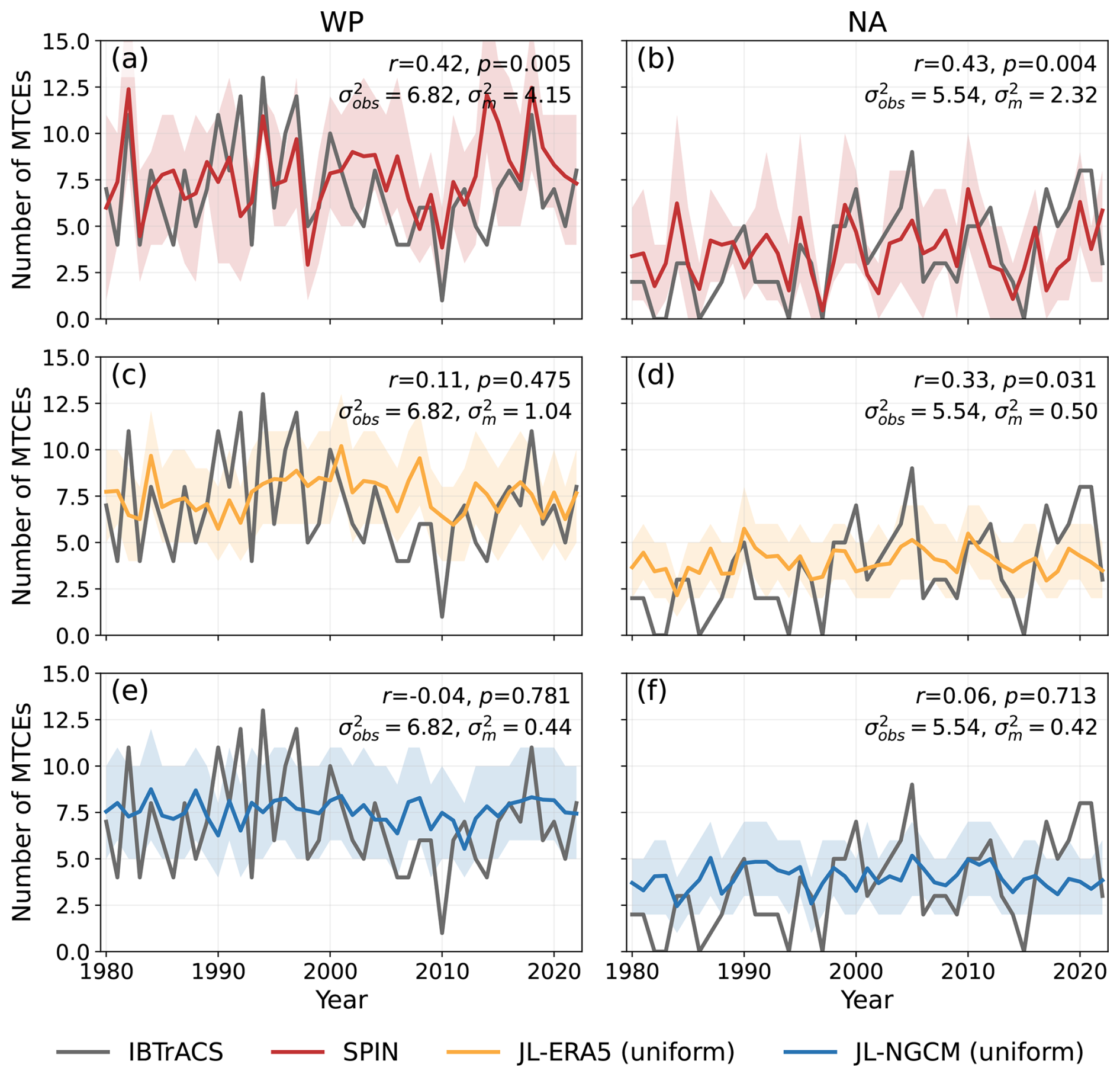
Figure 12 Interannual variability of multiple tropical cyclone events (MTCEs) in the WP and NA basins during 1980–2022. Results for IBTrACS are shown in black. The ensemble mean of SPIN simulations is shown in red (a–b), the JL23 model downscaling with uniformly sampled genesis dates is shown in yellow for ERA5 (c–d) and in blue for NeuralGCM (e–f). Shaded bands denote the 10th–90th percentile range. For SPIN, it represents the spread across ensemble members. For the “uniform” experiments, the range is estimated across 1000 Monte Carlo realizations. Pearson correlation coefficients (r), associated significance levels (p), and the variances of modelled and observed annual frequencies $\left({\mathit{\sigma }}_{\mathrm{m}}^{\mathrm{2}}\right.$ and $\left.{\mathit{\sigma }}_{\mathrm{obs}}^{\mathrm{2}}\right)$ are reported in the upper-right corner of each panel.

Next, we evaluate the distribution of MTCE cluster sizes, defined as the peak number of concurrent TCs within a cluster (see Sect. 2.5; Fig. 13). SPIN closely reproduces the observed distribution, with MTCEs most frequently exhibiting two peak concurrent TCs. The probability decreases with increasing numbers of concurrent TCs per MTCE cluster, and clusters with more than five concurrent TCs are rare. In contrast, uniform-date sampling methods, whether applied to IBTrACS, SPIN, or synthetic TCs generated by JL23 using NeuralGCM or ERA5 environmental inputs, generally overestimate the frequency of larger clusters, especially in the WP basin. This bias is consistent with the overrepresentation of short TC inter-genesis intervals within the 0–5 d bin under uniform-date sampling (Fig. 11), which artificially increases the likelihood of multiple TCs being included within the same cluster. The stronger contrast between the original and uniform-timing experiments in the WP basin than in the NA basin may reflect a greater role of intra-month to subseasonal variability in organizing TC genesis in the WP, although the underlying dynamical controls remain to be clarified. These results suggest that SPIN captures physically organized intra-month TC genesis timing, providing a more realistic basis for estimating MTCE cluster sizes than uniform-date sampling.

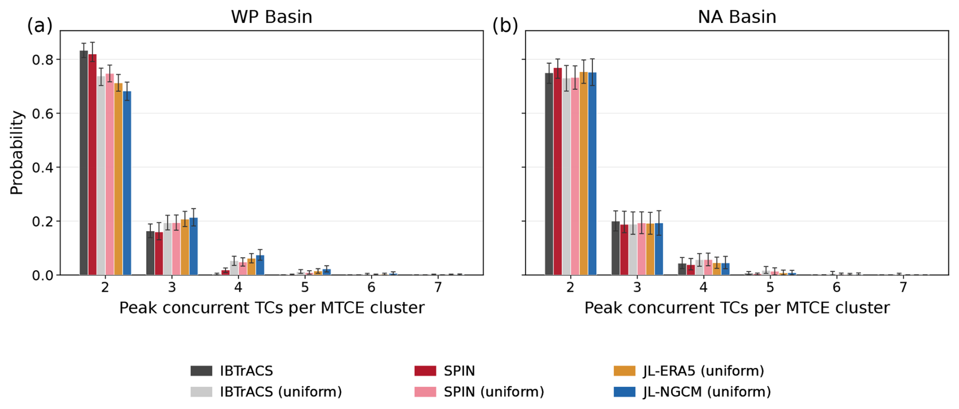
Figure 13 Histogram of MTCE cluster size for the (a) WP and (b) NA basins during 1980–2022. Cluster size is defined as the peak number of concurrent TCs within each MTCE cluster. The x-axis shows the peak concurrent TC count, and the y-axis shows the probability. Results are shown for IBTrACS (black), IBTrACS with uniformly sampled genesis dates (grey), the SPIN ensemble mean (red), SPIN with uniformly sampled genesis dates (pink), JL23 downscaling driven by ERA5 environmental fields with uniformly sampled genesis dates (yellow), and JL23 downscaling driven by NeuralGCM environmental fields with uniformly sampled genesis dates (blue). Error bars indicate the 10th–90th percentile range. For IBTrACS, the range is estimated by year bootstrapping over 1980–2022. For SPIN, it represents the spread across ensemble members. For the “uniform” experiments, the range is estimated across 1000 Monte Carlo realizations.

SPIN also well-captures the spatial pattern of MTCE compared to observation (Fig. 14). It reproduces the observed preference for subsequent TC genesis in the southeastern quadrant relative to the pre-existing TC (Krouse and Sobel, 2010; Yoshida and Ishikawa, 2013), with the fewest events occurring in the northwestern quadrant in the WP basin and in the northeastern quadrant in the NA basin. The agreement is particularly close in the WP basin, whereas in the NA basin SPIN shows a larger discrepancy, overestimating events in the southeastern quadrant and underestimating those in the southwestern quadrant (Fig. 14). For inter-storm distances (Fig. 15), SPIN reproduces the observed distribution in both basins, with fewest events at <1000 km, a peak at 2000–3000 km in the WP, and a peak at >4000 km in the NA. The overestimation of the >4000 km bin in the NA basin may reflect excess TC genesis near West Africa (Fig. 6), slightly longer simulated TC lifetimes (Fig. S9), or a combination of both.

Figure 14 Relative locations between pre-existing and subsequent TCs in MTCEs from 1980 to 2022 for the WP (a–b) and NA (c–d) basins. The crosshair center marks the pre-existing TC. Points in the four quadrants show the relative positions of subsequent TCs for IBTrACS (first column) and for SPIN (second column; all ensemble members with a single velocity initialization run). Percentages for each quadrant are reported. SPIN results include the 10th–90th percentile range.

Figure 15 Histogram of distances between pre-existing and subsequent TCs within MTCEs from 1980 to 2022. Panel (a) shows the global distribution, panel (b) the NA basin, and panel (c) the WP basin distributions. Results are binned into fixed 1000 km intervals. IBTrACS are shown in black bar, and the SPIN ensemble mean is shown in red with 10th–90th percentile ranges.

4 Return periods

In this section, we evaluate SPIN's skill in estimating return periods of metrics of interest at both global and regional scales. In particular, we investigated return periods of landfall intensity and the inter-event time between MTCEs.

4.1 Return period of landfall intensity

Figure 16 presents global maps of the return period for Category 1 and above TCs based on observations and SPIN downscaled results. SPIN successfully captures the main hazard hotspots, including the southwestern part of the western North Pacific, which covers southeastern China, southern Japan, and the Philippines, as well as the southeastern part of the eastern North Pacific. In these regions, return periods are generally less than 10 years and, in some areas, less than 5 years. Compared with observations, SPIN tends to overestimate hazard along the coasts of China, Japan, and the eastern United States, as indicated by shorter return periods, while underestimating hazard in some other regions, including India and the west coast of the United States, where return periods are longer than observed. These regional differences are broadly consistent with biases in simulated storm activity shown in Fig. 8 and may also reflect biases in the intensity simulations. It should be noted that, since TCs are rare events and the observational record is limited in duration, the observed hazard may not necessarily reflect the true underlying risk (Lee et al., 2018; Lin et al., 2023).

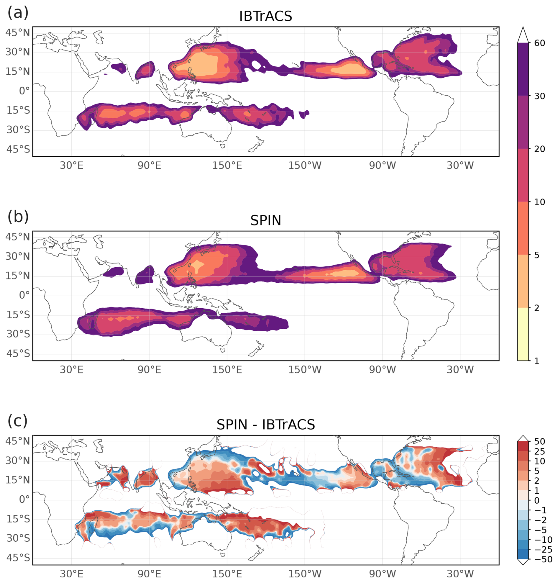
Figure 16 Global return period of TCs reaching ≥33 m s⁻¹ (Category 1): (a) IBTrACS, (b) SPIN ensemble mean, and (c) their difference on a 1°×1° grid with Gaussian smoothing. In panel (c), red (blue) indicates longer (shorter) return periods in SPIN than in IBTrACS, i.e., hazard underestimation (overestimation) by the model.

Next, we evaluate return period of landfall intensity for various TC-prone regions worldwide (Fig. 17). The curves are shown without regional bias correction. Overall, SPIN captures the observed order of magnitude of landfall return periods in most regions. Regional biases remain, with longer return periods in some regions such as the Bay of Bengal, Philippines, Australia and Madagascar, and shorter return periods in parts of China and the Eastern US. These biases likely reflect a combination of regional landfall-frequency biases and biases in landfall intensity. Because SPIN applies a single set of FAST parameters across regions, this configuration is not necessarily optimal for every region. For application-specific hazard assessments, targeted calibration of the FAST parameters may further improve regional estimates of landfall intensity return periods.

Figure 17 Return periods of landfall intensity for the following regions: Gulf of Mexico, Bay of Bengal, Eastern United States, Western Mexico, Caribbean Islands, China, Japan, Philippines, Australia, and Madagascar. Results from IBTrACS are shown in black, the solid blue line shows the return period curve computed from all ensemble members of SPIN combined (i.e., stacking all 14 members, 43 years, and 10 runs, yielding a total of 6020 years). The shaded region represents the 10th–90th percentile spread across all individual ensemble members.

4.2 Return period of MTCEs

Finally, we compare multi-model return periods for the intervals between MTCEs (Fig. 18). SPIN closely reproduces the observed return period in both basins, whereas JL-ERA5 and JL-NGCM underestimate the intervals, consistent with their weaker representation of MTCE occurrence. The IBTrACS-uniform baseline agrees with observations over the sampled range, but cannot constrain the tail because of the limited number of observed events. Moreover, because this approach does not simulate TCs based on environmental fields, it is difficult to extend to future climate scenarios. How MTCE recurrence changes under future climate scenarios, and which physical mechanisms control those changes, remain important questions for future work.

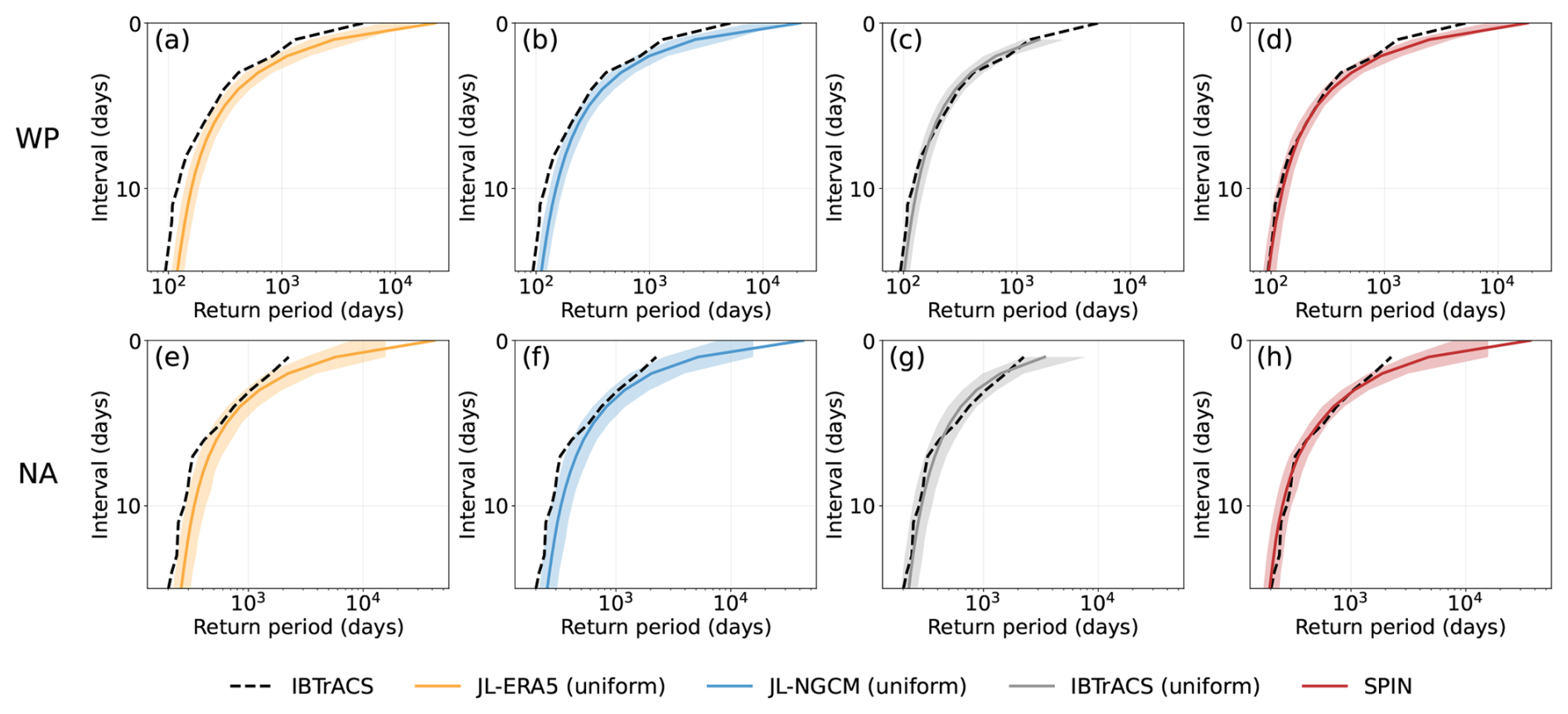
Figure 18 Return periods of inter-MTCE time. The y-axis shows the MTCE inter-genesis interval (0–15 d), and the x-axis shows the return period (days). Panels (a)–(d) correspond to the WP basin and panels (e)–(h) to the NA basin. Shown for comparison are results from IBTrACS (black), IBTrACS with uniformly sampled dates (grey), JL-ERA5 with uniformly sampled dates (yellow), and JL-NGCM (single ensemble member) with uniformly sampled dates (blue), and SPIN (red). The solid line in each panel indicates the return period computed from all Monte Carlo simulations (a, b, c, e, f, g) or all ensemble members (d, h). The shaded region represents the 10th–90th percentile range across individual ensemble members.

5 Summary and discussion

In this study, we develop a hybrid framework, SPIN, that functions as a spontaneous synthetic TC model with realistic intensity, to downscale TCs for risk analysis. The model leverages NeuralGCM (Kochkov et al., 2024) to simulate ensembles of spontaneously generated TC tracks, and couples the FAST intensity model (Emanuel, 2017; Lin et al., 2023) to compute realistic intensities based on the large-scale environment. In this way, SPIN bridges the gap between statistical and dynamical downscaling models and offers two key improvements over earlier statistical downscaling methods. First, it generates large ensembles of synthetic TCs together with their ambient environments. Second, it resolves intra-month processes. Therefore, SPIN advances TC risk assessment by enabling compound TC hazards, such as MTCEs and related events, to be assessed as dynamically organized events rather than statistical co-occurrences alone.

SPIN reproduces key features of observed TC climatology, including interannual variability of TC frequency, seasonal cycle, patterns of TC genesis and tracks, and the probability distribution of LMI. Compared with previous statistical downscaling models, SPIN better represents interannual variability in regions where ENSO signals are mixed (e.g. the WP and Southern Hemisphere basins). This improvement likely arises because SPIN diagnoses candidate storms from NeuralGCM-simulated evolving environmental fields, preserving year-to-year variations in both environmental favourability and the supply of precursor disturbances. By contrast, earlier synthetic TC models based on random seeding do not dynamically link seed supply to ENSO-related circulation changes. In addition, SPIN explicitly resolves intra-month processes so it can more realistically reproduces the distribution of inter-genesis intervals in each basin.

Beyond reproducing individual TC events, SPIN shows robust skills in simulating MTCEs. We evaluate SPIN's performance in reproducing MTCE characteristics in the WP and NA basins, where MTCEs occur most frequently (Fu et al., 2025). Compared with the benchmark models, SPIN better captures observed interannual variability, with higher correlations and a closer match to the observed variance. It also more accurately represents MTCE cluster size, consistent with its improved simulation of TC inter-genesis intervals. SPIN further captures the observed spatial distribution and return periods of MTCEs in both basins.

Several aspects can be improved in future work. For example, although the FAST intensity component reproduces the overall distribution of LMI reasonably well, it tends to underestimate rapid intensification and is therefore associated with a lower occurrence of intense TCs than observed. Moreover, TC intensity is diagnosed offline using FAST, and NeuralGCM is an atmosphere only model. Therefore, air–sea interactions related to storm intensity, such as storm induced cold-wake cooling, do not feed back onto the simulated environment or influence other TCs.

More broadly, SPIN demonstrates how hybrid AI-physics climate models can be used to build physically informed and computationally efficient hazard downscaling frameworks. Its modular design facilitates future model development. In particular, the framework can be readily integrated with other AI-based weather and climate models and is expected to benefit from improvements in the representation of large-scale climate variability. It could also be extended to investigate other compound hazards, such as TC-associated heatwaves, and coupled with GCM simulations to assess projected changes in TC and MTCE characteristics under future climate scenarios.