Resolving effects of leaf pigmentation changes and plant residue on the energy balance of winter wheat cultivation in the ORCHIDEE-CROP model

Crop management impacts climate not only through changes in carbon stocks and greenhouse gas budgets, but also through alterations in the surface energy budget. However, the latter aspect remains only partially represented in current cropping system models. Coupling dedicated crop models with land surface models provides a promising approach for quantifying these effects, but this effort is hindered by the simplistic representation of surface albedo as a combination of soil albedo and a static vegetation albedo controlled by vegetation cover. Here, we developed ORCHIDEE-CROP, a land surface model integrating the cropping system model STICS, by incorporating time-varying albedo from crop pigmentation during foliar yellowing and post-harvest crop residue soil cover. We further parameterized the effect of crop residues on surface roughness and soil evaporation affecting the surface energy budget and partitioning between latent and sensible heat fluxes. Using 10 site simulations, we quantified the impacts of these processes on soil temperature, soil moisture, water and heat fluxes of winter wheat crops. Incorporating foliar yellowing and post-harvest residue cover increased surface albedo by an average of 0.07 ± 0.03 during the foliar yellowing period and 0.02 ± 0.02 during the residue cover period, accordingly inducing surface cooling by −1.55 ± 0.93 and −1.90 ± 0.88 °C. During each period, sensible heat flux changed by −8.10 ± 4.18 and −7.44 ± 3.98 W m⁻², while latent heat flux decreased by −6.84 ± 1.41 and −5.15 ± 4.03 W m⁻². The spatiotemporal variability of these effects was driven by site-specific meteorology and soil properties. Simulations under dry scenarios reveal that crop residues left on the field can progressively increase plant-available water over multiple years under dry conditions. This study underscores that crop pigmentation has a minor influence on water–heat processes, while residues moderately modulate surface energy partitioning with significant spatial heterogeneity, highlighting the potential of residue management for climate mitigation. The refined modelling framework enables simultaneous assessment of the biogeochemical and biophysical impacts of field operations on the Earth System.

1 Introduction

Agriculture and climate are interconnected by greenhouse gas, energy and water budgets (IPCC, 2014; Wu et al., 2016; Chen et al., 2024). These interactions create a dual challenge that agricultural systems are both vulnerable to climate change impacts (e.g., droughts, extreme weather) and significant contributors to global emissions. Adaptive management practices are therefore critical for enhancing agricultural resilience and sustainability while simultaneously reducing anthropogenic disturbances to the environment and climate. To quantify the complex spatiotemporal climate impacts of management practices, coupling land surface models with dedicated crop modules represents a promising strategy. These models are effective tools for simulating biophysical and biogeochemical processes at the agriculture–climate interface, such as crop physiological growth, yield dynamics, and the exchange of carbon, water, and energy between agroecosystems and the atmosphere (Brisson et al., 2003; Fisher et al., 2014; McDermid et al., 2017). By capturing these processes, land surface models provide essential insights for projecting future climate-agriculture feedback under varying management scenarios (Arora et al., 2023; Timlin et al., 2024). However, a key limitation arises from the inconsistency between the diversity and complexity of real-world agricultural management practices and their overly simplistic representations in current land surface models. This gap significantly hinders the ability of land surface models to reliably predict climate impacts, particularly at regional or farm-specific scales where management decisions are highly required (Fisher and Koven, 2020). A key example of the limited ability of land surface models in representing biophysical processes of agriculture–climate interactions is their treatment of crop albedo dynamics.

Surface albedo, as the fraction of incoming solar radiation that is reflected by the soil and crops, plays a critical role in both radiative and non-radiative climate processes (Seneviratne et al., 2018; Zhang et al., 2022a). Crops and their residues exhibit distinct albedo due to differences in plant traits (e.g., leaf pigmentation, canopy structure) and management practices (e.g., tillage, residue retention, irrigation). For example, existing research shows an averaged albedo of 0.16–0.19 for winter wheat (Şerban et al., 2011; Sieber et al., 2022; Lei et al., 2024), of 0.18–0.20 for soybean (Costa et al., 2007; Lei et al., 2024), and of 0.15–0.18 for corn (Jacobs and van Pul, 1990; Lei et al., 2024). These differences in albedo directly affect global climate by changing the radiative forcing at the top of the atmosphere (Stephens et al., 2015). In addition, changes in surface albedo modify the surface energy balance, potentially redistributing energy between latent and sensible heat fluxes through non-radiative processes. However, land surface models generally use simplistic parameterizations of static soil and crop albedo. When temporal dynamics are included, they are typically limited to changes in the fractional coverage of soil and vegetation (Dalgliesh et al., 2016; Wu et al., 2016; Hoogenboom et al., 2024). Because they lack mechanisms to represent changes in crop pigmentation, these models are poorly suited to quantify climate effects of managements or crop breeding which affect crop residue or crop pigmentation (e.g., no tillage, pale crops) (Drewry et al., 2014).

Winter wheat, as a major cereal crop, undergoes distinct phenological stages that are accompanied by changes in canopy pigmentation and surface reflectance (Zhang et al., 2022b). During its growth cycle, winter wheat transitions from chlorophyll-dominated green leaves to senescent yellow leaves after maturity, where reduced chlorophyll levels expose light-reflecting carotenoids (Féret et al., 2017). Additionally, crop residues left on the field after harvest introduce additional albedo variability compared with bare soil in conventional tillage systems, with the extent of this fluctuation depending on the baseline bare soil albedo and residue management practices (Simão et al., 2021). Generally higher albedo of vegetation than bare soil in most croplands in Europe possibly induces an increase in surface albedo when covering residues on the soil (Pique et al., 2023). Such physiological development of winter wheat and residue coverage therefore affect the climate through changes in surface albedo, potentially offsetting part of the warming caused by greenhouse gas emissions. However, it is difficult for current land surface models to quantify and evaluate these effects because they are generally ignored or parameterized using simplified assumptions (Davin et al., 2014; Sieber et al., 2022; Yu et al., 2024).

This study simulates the biophysical impacts of winter wheat phenology and residue management on surface energy balance through albedo-mediated processes in the ORCHIDEE-CROP land surface model. To achieve this, we improved the model by refining the representation of foliar pigmentation and crop residue effects on albedo dynamics, as well as their influence on soil evaporation and surface roughness based on observations from 10 European cropland sites. Section 2 details the datasets and methodology used for model parameterization. We briefly review the baseline modeling representation of surface albedo, hydrology, roughness, and energy fluxes before introducing our modifications in ORCHIDEE-CROP. These improvements enhance the representation of albedo dynamics, soil evaporation, and surface roughness, with two simulations for evaluating the albedo-mediated impact of residue retention conducted under both current and dry scenarios. Section 3 presents the results of these refinements, while Sect. 4 analyses the contribution of albedo changes, driven by foliar pigmentation and crop residues, on modulating surface temperature, latent heat, and sensible heat fluxes. We also discuss the potential of crop residue management for climate adaptation and mitigation. Finally, Sect. 5 summarizes our findings and conclusions. By incorporating albedo dynamics influenced by crop pigmentation and residue management, this study enhances the realism of coupled cropland surface models and demonstrates its impacts on field-level energy balance under present and future idealised climate.

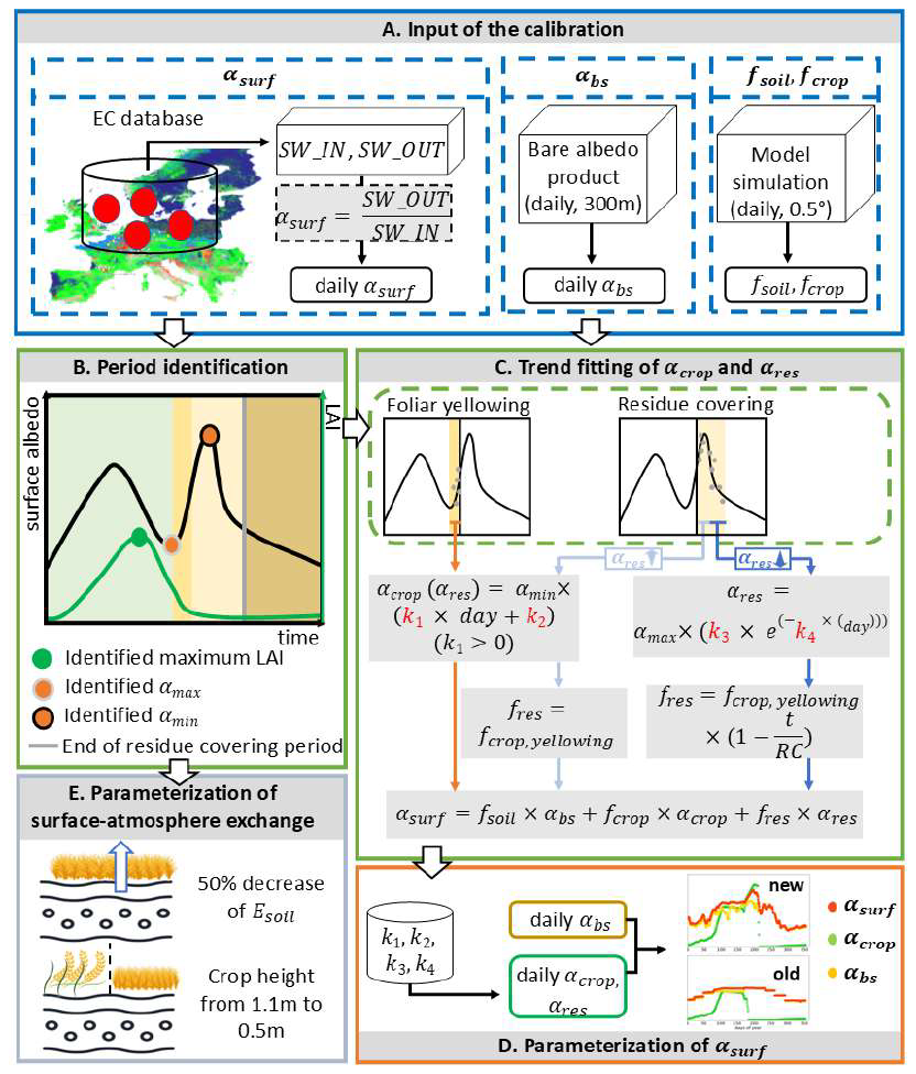
Figure 1 The procedure of parameterization of crop and residue albedo (α_surf and α_res), soil evaporation (E_soil) and surface roughness (Z₀) in the ORCHIDEE-CROP model. Panel (A) illustrates the input datasets for albedo calibration. α_soil and α_surf are bare soil albedo (α_soil) and surface albedo (α_surf), respectively. f_crop and f_soil are the gridded fractions of crop (f_crop) and residues (f_res), respectively. SW_IN and SW_OUT are half-hourly incoming (SW_IN) and outgoing (SW_OUT) solar radiance observed at seven eddy-covariance (EC) sites. Panel (B) shows the identification of foliar yellowing and residue covering periods based on time series of α_surf (black curve) and leaf area index (LAI, green curve). α_min and α_max are the identified minimum and maximum α_surf. The shallow-green, orange, yellow and brown areas show the conceptual growing, maturity, residue covering and bare soil periods of winter wheat. Panel (C) describes trend fittings for crop albedo (α_crop) and α_res. Features in two plots have the same meanings with the ones in Panel (B). f_{crop,yellowing} is the fraction of crop during the foliar yellowing period. RC is the duration of residue covering. k₁, k₂, k₃ and k₄ are the fitting parameters during foliar yellowing and residue covering periods. Day and t are the days of α_surf increase during residue covering period. Panel (D) illustrates parameterization of α_surf as a weighted combination of α_crop, α_res and α_soil in ORCHIDEE-CROP model. The daily α_surf in orange in the upper plot is derived from the new calibrated process based on k₁–k₄, compared to the old model (plot below). Panel (E) presents parameterization of surface–atmosphere exchange. E_soil is the soil evaporation and the dotted vertical line represents the harvesting date of winter wheat.

2 Data and methods

The improvements of the ORCHIDEE-CROP model are illustrated in Fig. 1 and structured into six subsections: (1) Datasets (Sect. 2.1); (2) Introduction of the ORCHIDEE-CROP model (Sect. 2.2); (3) New parameterization of the ORCHIDEE-CROP model (Sect. 2.3); (4) Model calibration (Sect. 2.4); (5) Model simulations (Sect. 2.5); (6) Model evaluation (Sect. 2.6).

2.1 Datasets

2.1.1 Daily surface albedo from site observation

To derive surface albedo (α_surf, unitless) from site observations, we combined datasets from two sources: (1) eddy-covariance measurements from the Integrated Carbon Observation System (ICOS) Data Portal (Dumont et al., 2024; Schmidt et al., 2025; Buysse et al., 2023; Brut et al., 2024; Brümmer et al., 2023; Tallec et al., 2026; Bernhofer et al., 2026), and (2) satellite-derived products at farms belonging to the ClieNFarm project. From the ICOS network, we obtained the half-hourly incoming and outgoing solar radiance (SW_IN and SW_OUT, W m⁻²) measurements from 2000 to 2020 at eight wheat cultivated sites (BE-Lon, CH-Oe2, DE-Geb, DE-Kli, DE-RuS, FR-Aur, FR-Gri, FR-Lam) (Fig. S1 in the Supplement). Data were quality-controlled and gap-filled using uniform methods (Pastorello et al., 2020). Details of the quality filtering and preprocessing procedures of α_surf are provided in Sect. S1.1 in the Supplement. The daily shortwave mid-day α_surf was calculated from average values of SW_IN and SW_OUT from 11:00 to 13:00 Central European Summer Time at each site (Lin et al., 2023):

$$\begin{array}{}\text{(1)}& {\mathit{\alpha }}_{\text{surf}}={\displaystyle \frac{\text{SW\_OUT}}{\text{SW\_IN}}}\end{array}$$

At six farms across two ClieNFarm sites (UK-Rookery, UK-Winwick, UK-Allerton, BE-AH, BE-BM, BE-LB) where direct radiation measurements were unavailable, we estimated surface albedo at 5 d intervals and 300 m resolution using Sentinel-2 (S2) reflectance data. A 10 % cloud-cover threshold was applied for quality filtering, and retrievals followed the framework developed by Lin et al. (2023). For the selected 10 sites, we chose only the years during which winter wheat was cultivated, and obtained a total of 33 winter wheat years.

2.1.2 Meteorological data from site observation

We utilized the half-hourly meteorological observations from flux towers in the winter wheat years at eight ICOS sites to force the ORCHIDEE-CROP model. The observations include SW_IN, surface pressure (Pa), near-surface specific humidity (kg kg⁻¹), rainfall rate (kg m⁻² s), snowfall rate (kg m⁻² s), near-surface air temperature (K), and near-surface eastward and northward wind components (m s⁻¹). The FLUXNET_DATA tool (available upon request from the authors) was used to fill gaps in the flux-towers data using 6-hourly ERA-interim products (Vuichard and Papale, 2015). We then averaged all gap-filled variables to a 6 h time step to meet the input requirements of the model. At the two ClieNFarm sites without flux observations, the meteorological variables from the hourly 0.25° ERA-interim product were extracted and interpolated to exact site coordinates to provide meteorological forcing data.

In 10-year simulations for the current climate scenario from 2010 to 2020 (Sect. 2.5), the processed climate forcing data from each year obtained from the ICOS Data Portal was used to drive the model. For the dry scenario, the driest year at each site was identified based on the lowest annual precipitation. All meteorological variables from this year were then used to force the simulation. This approach ensures that the dry scenario is driven by a coherent and physically realistic set of meteorological conditions. Yearly-averaged meteorological variables in the driest year for each site are presented in Table S1 in the Supplement.

2.1.3 Management practice, bare soil albedo and LAI

Management practices during the winter wheat cultivation year at all sites (Table S2 in the Supplement) were obtained from a crop management database provided by site managers. Key practices, including sowing, harvesting, and tillage dates, were prepared as input for the ORCHIDEE-CROP model.

Bare soil albedo (α_soil, unitless) was prescribed using a high-resolution 5 d, 300 m European α_soil dataset derived from 10 m S2-α_surf observations covering the period 2018–2020 (Yu et al., 2026). This dataset demonstrated sufficient skill in resolving daily soil dynamics at the field scale in fragmented European croplands. Since the model was run at the site scale, bare soil albedo values were extracted for each site location, and linear interpolation was applied to convert the data to a daily time step, aligned with the model temporal resolution.

Due to the absence of sporadic leaf area index (LAI, m² m⁻²) measurements found at ICOS sites (Table S3 in the Supplement), we used continuous satellite-based LAI datasets to identify the timing of peak LAI at those sites. LAI at each site was extracted from the 4 d, 500 m LAI product from the MODIS (MCD15A3H) (Myneni et al., 2015). Daily LAI dynamics were derived through linear interpolation combined with a Savitzky–Golay filter (window length = 15) to smooth the trend and remove the outliers. MODIS-derived LAI was used to constrain the onset of crop maturity period, rather than to reproduce absolute LAI values. The LAI comparison between MODIS product and site measurements is shown in Fig. S2 in the Supplement. We used the MODIS-derived LAI product rather than the S2-derived product, because the temporal coverage of the latter is insufficient to match the available site observations.

2.2 Introduction of the ORCHIDEE-CROP model

The ORCHIDEE-CROP model is a branched version of the process-based land surface model, ORCHIDEE (Krinner et al., 2005), which incorporates a generic crop phenology and harvest module, along with simplified nitrogen fertilization parameterization based on the process-based STICS formalism (Wu et al., 2016). It simulates biophysical and biogeochemical interactions in croplands, as well as plant productivity and harvested yield. A detailed model description is available in Wu et al. (2016). This study employs a previously developed model version calibrated against LAI, flowering and harvesting dates, and crop yield for both winter wheat and maize (https://github.com/yangsssu/ORCHIDEE-CROP.git, last access: 13 February 2026). In the present study, only winter wheat is considered. The derived climate and management information were used to drive the model as forcing data (Sect. 2.1.2 and 2.1.3). Winter wheat is the only vegetation type considered in this analysis. To assess the impacts of winter wheat physiological development and residue coverage on the surface energy balance and water–energy fluxes, we describe below the key processes governing surface energy balance (Sect. 2.2.1), α_surf dynamics (Sect. 2.2.2), hydrology (Sect. 2.2.3), the surface roughness (Sect. 2.2.4), as well as crop growth and development (Sect. 2.2.5).

2.2.1 Surface energy balance

The ORCHIDEE-CROP model simulates the surface energy budget by:

$$\begin{array}{}\text{(2)}& R_{\mathrm{n}}=LE+H+G\end{array}$$

where the net radiation (R_n, W m⁻²) governs land–atmosphere water and heat exchange, driven by the partitioning of LE, sensible heat fluxes (H, W m⁻²) and soil heat fluxes (G, W m⁻²). R_n is determined by the net short-wave radiation budget (S_n, W m⁻²) and the net long-wave radiation budget (L_n, W m⁻²) (Ducoudré et al., 1993).

$$\begin{array}{}\text{(3)}& R_{\mathrm{n}}=S_{\mathrm{n}}+L_{\mathrm{n}}=(\mathrm{1}-{\mathit{\alpha }}_{\text{surf}})\times \text{SW\_IN}+L\downarrow -L\uparrow \end{array}$$

where L↓ is the down-welling longwave radiation (a model input variable). L↑ is the upwelling longwave radiation emitted by the land surface, which is estimated by surface temperature (T_surf, K) (a model input variable) based on Stefan–Boltzmann law.

Because α_surf directly influences R_n, its formulation in the ORCHIDEE-CROP model is described below.

2.2.2 Surface albedo dynamics

The model calculates α_surf in step t for both the visible and near-infrared domains by the area-weighted sum of foliar albedo (α_crop, unitless) and α_soil:

$$\begin{array}{}\text{(4)}& {\mathit{\alpha }}_{\text{surf}}\left(t\right)=(\mathrm{1}-f_{\text{crop}}(t\left)\right)\times {\mathit{\alpha }}_{\text{soil}}\left(t\right)+f_{\text{crop}}\left(t\right)\times {\mathit{\alpha }}_{\text{crop},\text{constant}}\end{array}$$

where f_crop(t) and 1−f_crop(t) represent the fractions of winter wheat and bare soil covering the surface area of the model pixel; α_{crop,constant} of winter wheat is set as the default value of 0.1 and 0.3 for visible and near-infrared ranges of α_crop, respectively. α_soil(t) is derived from daily α_soil dataset (Sect. 2.1.3). Since α_surf affects radiation absorption, it influences soil moisture availability and, consequently, soil evaporation (E_soil).

2.2.3 Hydrology

The ORCHIDEE-CROP model computes soil water budget by considering the three reservoirs of canopy interception, snow packing and 11 soil layers (MacBean et al., 2020). The water fluxes at soil surface include water inputs from throughfall, snowmelt and irrigation, and water output from soil by surface runoff, bare soil evaporation and drainage. Here, we mainly describe the calculation of E_soil and the soil water content (SWC, kg m⁻²) in different soil layers.

The ORCHIDEE-CROP model calculates LE by accounting for snow sublimation, canopy interception and transpiration, E_soil and floodplain evaporation. A β-model is used to compute E_soil by inducing a series of aerodynamic and surface resistances.

$$\begin{array}{}\text{(5)}& \begin{array}{rl}{E}_{\text{soil}}\left(t\right)=& (\mathrm{1}-{\mathit{\beta }}_{\mathrm{1}})\times (\mathrm{1}-{\mathit{\beta }}_{\mathrm{5}})\times {\mathit{\beta }}_{\mathrm{4}}\times r_{\text{au}}\times v\times C_{\text{d}}\\ & \times (q_{\text{surf}}-q_{\text{air}})\times \mathrm{d}t\end{array}\end{array}$$

where β₁, β₄ and β₅ are dimensionless scaling factors representing soil moisture and surface resistance effects for snow sublimation (β₁), soil evaporation (β₄) and floodplain evaporation (β₅), respectively; r_au (kg m⁻³), v (m s⁻¹), C_d (–), q_surf (kg kg⁻¹), and q_air (kg kg⁻¹) are the air density, wind speed, drag coefficient, saturated surface air moisture, and specific humidity, respectively. The bulk formulation yields evaporation in $\mathrm{kg}{\mathrm{m}}^{-\mathrm{2}}{\mathrm{s}}^{-\mathrm{1}}$, which is integrated over the model time step (dt) to obtain values in kg m⁻². This quantity is then expressed in mm d⁻¹ using the equivalence 1 mm = 1 kg m⁻².

Soil moisture dynamics are governed by a diffusive multi-layer soil hydrology scheme with 27 soil layers (up to 2 m), based on moisture diffusion principles (Richards, 1931; de Rosnay et al., 2002; Wu et al., 2016). It uses the 1D Richards equation with soil volumetric water content as the state variable in its saturated form, instead of the pressure head (Campoy et al., 2013).

2.2.4 Surface roughness

Surface roughness (Z₀, m) plays a critical role in regulating near-surface turbulence and the water–heat exchange process between the land surface and the atmosphere (Meier et al., 2022; Chen et al., 2024). E_soil depends on Z₀, which modulates atmospheric turbulence and moisture transfer. The ORCHIDEE-CROP model uses the averaged drag coefficients for momentum and heat transfer over winter wheat to compute the grid-averaged roughness height.

$$\begin{array}{}\text{(6)}& Z_{\mathrm{0}}\left(t\right)=f_{\text{crop}}\left(t\right)\times {\left({\displaystyle \frac{C_{\mathrm{k}}}{\left(\frac{Z_{\text{tmp}}}{max(H_{\mathrm{c}}\times Z_{\mathrm{0},\mathrm{h}},Z_{\mathrm{0},\text{bare}})}\right)}}\right)}^{\mathrm{2}}\end{array}$$

where Z₀(t) is the daily roughness height over each grid cell. C_k (–) is the von Karman constant, which equals to 0.41. Z_tmp (m) represents the maximum height of the first atmospheric layer and is determined by air pressure, air temperature, and air density. This variable represents the reference height used for flux calculations and is set to a minimum of 10 m above the ground. This ensures that the reference height remains above the canopy height, thereby maintaining the stability of the logarithmic function used in flux calculations. H_c (m) represents winter wheat height, which is treated as a time-invariant constant and set to 1.1 m in the ORCHIDEE-CROP model. For comparison, the maximum H_c of winter wheat during growing seasons measured at five sites has an average of 0.97 m (Table S3). Z_0,h equals to $\mathrm{1}/\mathrm{16}$, which is utilized to estimate the roughness height above the canopy. Z_0,bare (m) is set as 0.01 m for roughness length of bare soil. Z₀ for the bare soil can be derived by:

$$\begin{array}{}\text{(7)}& Z_{\mathrm{0}}\left(t\right)=(\mathrm{1}-f_{\text{crop}}(t\left)\right)\times {\left({\displaystyle \frac{C_{\mathrm{k}}}{\left(\frac{Z_{\text{tmp}}}{Z_{\mathrm{0},\text{bare}}}\right)}}\right)}^{\mathrm{2}}\end{array}$$

The ORCHIDEE-CROP model computes a grid effective roughness height (H_rough, m) for deriving water–heat fluxes. It combines the zero-plane displacement height (Z_dis, m) which is an equivalent height for the absorption of momentum, and the vegetation height weighted by the maximum f_crop ($f_{\text{crop},max}$) of winter wheat within each grid (H_ave, m):

$$\begin{array}{}\text{(8)}& {\displaystyle }& {\displaystyle }{H}_{\text{rough}}=H_{\text{ave}}-Z_{\text{dis}}\text{(9)}& {\displaystyle }& {\displaystyle }{Z}_{\text{dis}}=H_{\text{ave}}\times H_{\text{dis}}\text{(10)}& {\displaystyle }& {\displaystyle }{H}_{\text{ave}}=f_{\text{crop},max}\times H_{\mathrm{c}}\end{array}$$

H_dis (m) is used to determine the Z_dis based on H_ave, which equals to 0.75.

2.2.5 Crop growth and development

Crop development in the ORCHIDEE-CROP model is based on the crop model STICS (Wu et al., 2016). For winter wheat, the crop module simulates nine developmental stages of crop growth and grain filling (Fig. 2.1 in Brisson et al., 2003). The timing and duration of each developmental stage are calculated based on growing degree days adjusted by limiting functions related to photoperiod, vernalization and environmental constraints (e.g., water and nitrogen). Transitions between stages occur when the threshold values of growing degree days are reached.

In our simulations, sowing dates were prescribed using observed, site-specific management information to ensure consistency with field observations. Subsequent phenological development, including flowering, maturity, and harvest, is driven by growing degree days following the ORCHIDEE-CROP phenology scheme which was calibrated using extensive wheat phenology records from 1941 DWD climate stations across Germany (Su et al., 2025). This approach ensures that modeled flowering and harvesting dates are on average, consistent with observed phenology across a wide range of environmental conditions. We further adjusted the delay between crop maturation and harvest at each site using observed harvest dates which vary depending on management practices and weather conditions (Table S2).

2.3 New parameterization of the ORCHIDEE-CROP model

Foliar yellowing of winter wheat after maturation and crop residues remaining on the field after harvest affect α_surf and turbulent fluxes, but these processes are not currently represented in the model. As such, the absence of these key processes presents a gap in understanding and modeling of the impacts of winter wheat on regional energy and water cycles. We enhanced the ORCHIDEE-CROP model by introducing empirical functions describing temporal dynamics of α_surf, β₄ and Z₀ as a function of time, f_crop and f_res for foliar yellowing and crop residues. In addition, to ensure consistency between simulated and observed crop development periods (from sowing to harvest) at each site, the duration between maturity and harvesting in ORCHIDEE-CROP was calibrated using recorded harvesting dates at each site. In each winter wheat year at each site, simulations were performed iteratively with potential maturity-harvest intervals ranging from 5 to 40 d at 2 d increments. The optimal duration for each case was identified when the simulated harvest date matched the recorded management date. The calibrated durations are summarized in Table S2. It means that the site-specific durations of foliar yellowing before harvesting vary across all sites in the new model, compared to the default 14 d in the old model.

The objective of this model development targets a realistic mean effect size expected among European croplands, rather than capturing in detail the site-specific effects. We focus on improving the representation of albedo properties of winter wheat during the foliar yellowing and residue covering period, while associated impacts on surface energy fluxes are evaluated qualitatively rather than through a full recalibration of the hydrological scheme.

2.3.1 Improving albedo dynamics during the foliar yellowing periods

The foliar yellowing period in this model is defined as starting from the maturity date (nmat) and ending on the harvesting date based on analysis of observed α_surf dynamics at 10 sites (Sect. 2.4.1).

We replaced Eq. (4) with an equation which uses time-varying α_crop(t) instead of a α_{crop,constant}:

$$\begin{array}{}\text{(11)}& {\mathit{\alpha }}_{\text{surf}}\left(t\right)=(\mathrm{1}-f_{\text{crop}}(t\left)\right)\times {\mathit{\alpha }}_{\text{soil}}\left(t\right)+f_{\text{crop}}\left(t\right)\times {\mathit{\alpha }}_{\text{crop}}\left(t\right)\end{array}$$

To simulate the increase in α_crop after maturation and before harvesting we chose the following function:

$$\begin{array}{}\text{(12)}& {\mathit{\alpha }}_{\text{crop}}\left(t\right)={\mathit{\alpha }}_{\text{yellowing},\text{start}}\times (k_{\mathrm{1}}\times t+k_{\mathrm{2}})\end{array}$$

Where α_{yellowing,start} is the simulated α_crop on the first day during the foliar yellowing period. k₁ and k₂ represent the fitting parameters that are calibrated at the multi-site scale (see below).

Here, we assumed that f_crop remains constant during the foliar yellowing periods (f_{crop,yellowing}).

2.3.2 Improving albedo dynamics during the residue covering periods

The residue covering period starts from the harvesting date and ends either 90 d after harvesting, or earlier if tillage occurs (Sect. 2.4.1). As α_surf continuously increases after harvesting due to the presence of light-colored and evenly distributed straws, we used the segmentation function to describe α_surf dynamics from increase and subsequent decrease in α_surf during this period.

The α_surf at each time step can be represented by the area-weighted sum of α_soil and α_res:

$$\begin{array}{}\text{(13)}& {\displaystyle }{\mathit{\alpha }}_{\text{surf}}\left(t\right)=(\mathrm{1}-f_{\text{res}}(t\left)\right)\times {\mathit{\alpha }}_{\text{soil}}\left(t\right)+f_{\text{res}}\left(t\right)\times {\mathit{\alpha }}_{\text{res}}\left(t\right)\text{(14)}& {\displaystyle }\left\{\begin{array}{ll}{\mathit{\alpha }}_{\text{res}}\left(t\right)={\mathit{\alpha }}_{\text{yellowing},\text{start}}\times (k_{\mathrm{1}}\times t+k_{\mathrm{2}})& t\text{ in\hspace{0.17em}\hspace{0.17em}albedo}\\ & \text{increase}\\ & \text{phase};\\ {\mathit{\alpha }}_{\text{res}}\left(t\right)={\mathit{\alpha }}_{max}\times \left(k_{\mathrm{3}}\times e^{-k_{\mathrm{4}}\times t}\right)& t\text{ in\hspace{0.17em}\hspace{0.17em}albedo}\\ & \text{decrease}\\ & \text{phase};\\ {\mathit{\alpha }}_{\text{res}}\left(t\right)=\mathrm{0}& \text{otherwise};\end{array}\right.\end{array}$$

Where α_max is the simulated α_crop on the last day of the albedo increase phase. (1−f_res(t)) represent the daily variation of bare soil fraction. k₃ and k₄ represent the fitting parameters that need to be calibrated at the site scale (see below).

Here, f_res during the albedo increase phase equals to f_{crop,yellowing} and linearly decreases during the albedo decrease stage from f_{crop,yellowing}:

$$\begin{array}{}\text{(15)}& \left\{\begin{array}{ll}\mathit{\left\{}{f}_{\text{res}}\right(t)=f_{\text{crop},\text{yellowing}}& t\text{ in albedo}\\ & \text{increase}\\ & \text{phase};\\ f_{\text{res}}\left(t\right)=f_{\text{crop},\text{yellowing}}\times \left(\mathrm{1}-\frac{t}{\text{RC}}\right)& t\text{ in albedo}\\ & \text{decrease}\\ & \text{phase};\\ f_{\text{res}}\left(t\right)=\mathrm{0}& \text{otherwise};\end{array}\right.\end{array}$$

RC is the maximum residue covering period, either equals to 90 d or the tillage date.

2.3.3 Considering the impact of crop residue on soil evaporation during the residue covering periods

Crop residues covering part of soil surface decrease E_soil by increasing the soil-to-atmosphere resistance (Horton et al., 1996). The current ORCHIDEE-CROP model does not consider the impact of crop residue on E_soil. Previous site-scale observations generally show a 20 %–50 % reduction in E_soil in the presence of wheat residue compared with bare soil (Unger and Parker, 1968; Lascano and Baumhardt, 1996; Ramos et al., 2024). Based on Eq. (5), we assumed a maximum initial reduction in soil conductance (β₄, unitless) of 50 % under the highest f_res (Zhao et al., 2020; Raes et al., 2022), with a progressive increase of conductance as daily f_res declines during the residue cover period:

$$\begin{array}{}\text{(16)}& \begin{array}{rl}{E}_{\text{soil}}\left(t\right)=& (\mathrm{1}-{\mathit{\beta }}_{\mathrm{1}}(t\left)\right)\times (\mathrm{1}-{\mathit{\beta }}_{\mathrm{5}}(t\left)\right)\times (\mathrm{1}\text{–}\mathrm{0.5}\\ & \times f_{\text{res}}\left(t\right))\times {\mathit{\beta }}_{\mathrm{4}}(t)\times r_{\text{au}}(t)\times v(t)\times C_{\text{d}}(t)\\ & \times \left(q_{\text{surf}}\right(t)-q_{\text{air}}(t\left)\right)\times \mathrm{d}t\end{array}\end{array}$$

The meanings of all variables are the same as the ones in Eq. (5).

Note that β₄ represents an empirical resistance factor and cannot be directly inferred from observations. Therefore, its value was constrained through sensitivity testing against published experimental reductions in E_soil rather than calibrated directly using site-level flux measurements (Fig. S3 in the Supplement, Table S4 in the Supplement).

2.3.4 Considering the impact of crop residue on surface roughness during the residue covering periods

The initial version of the ORCHIDEE-CROP model assumed that Z₀ after harvest equals to that of bare soil coverage, omitting that (parts of the) stalks remain. To represent the impact of crop residues on Z₀ during the residue covering periods, we assumed that the H_c of plant changes from 1.1 m for winter wheat to 0.5 m for crop residues which has been identified as an optimal cutting height for harvest efficiency and soil and water conservation (MacMaster et al., 2000). f_crop is replaced with f_res. The new Z₀ and H_rough are therefore computed by:

$$\begin{array}{}\text{(17)}& {\displaystyle }{Z}_{\mathrm{0}}\left(t\right)=f_{\text{res}}\left(t\right)\times {\left({\displaystyle \frac{C_{\mathrm{k}}}{\left(\frac{Z_{\text{tmp}}}{max(\mathrm{0.5}\times Z_{\mathrm{0},\mathrm{h}},Z_{\mathrm{0},\text{bare}})}\right)}}\right)}^{\mathrm{2}}\text{(18)}& {\displaystyle }{H}_{\text{rough}}=f_{\text{crop},max}\times \mathrm{0.5}-f_{\text{crop},max}\times \mathrm{0.5}\times H_{\text{dis}}\end{array}$$

These two formulations remain identical to Eqs. (7) and (8), but with adjusted parameter values for canopy height and fractional cover to represent crop residues.

2.4 Model calibration

The parameters of α_surf dynamics were calibrated using data from 10 sites with 33 winter wheat site-years. α_surf and LAI observations were applied to identify foliar yellowing and residue covering periods at the available sites (Table S2).

2.4.1 Identifying the periods of foliar yellowing and residue covering from site observation

At the site scale, we assumed that foliar yellowing (i.e., α_surf increase) begins at crop maturity because no observational evidence supports a temporal gap between these two phases.

In the model, α_surf starts to increase after a delay following the maximum LAI and decreases after harvest. Post-harvest α_surf dynamics were divided into two phases: (1) an initial α_surf increase driven by light-colored, evenly distributed straw, followed by (2) a α_surf decline due to the dominating effects of decomposition of residues.

α_surf dynamics were parameterized by identifying critical temporal thresholds. The minimum α_surf between the LAI peak and harvest was used to define the onset of foliar yellowing, which is approximately 22.3 d (95 % bootstrap CI: [20.6–23.6] d, n=33) pre-harvest computed by site observation. This delay is longer than the default 14 d interval between maturity and harvest used in the old ORCHIDEE-CROP model. The maximum α_surf, constrained to occur within 30 d after harvest, divided residue-driven α_surf dynamics into an increasing phase (harvest to maximum α_surf) and a decline phase from post-maximum α_surf to tillage. Without tillage, the residue covering period was assumed to persist for 90 d after harvest (Kriaučiūnienė et al., 2012). On average, the maximum α_surf occurs 13.4 d (95 % bootstrap CI: [10.5–15.9] d, n=33) after harvest based on site identification, while the configuration in the old ORCHIDEE-CROP model does not consider the timing of maximum α_surf. Due to the lacking information of maximum α_surf during residue covering period in the old model, we utilized 15 d after harvesting as the boundary of these two phases in the ORCHIDEE-CROP model at all sites for simplification.

2.4.2 Parameter optimization of albedo dynamics

Daily α_surf and α_soil observations, together with information on bare soil exposure, were utilized to calibrate the empirical parameters k₁, k₂, k₃ and k₄ for α_crop and α_res (Eqs. 12 and 14). The α_{yellowing,start} (Eq. 12) was replaced by the α_surf observation at the beginning of the foliar yellowing period. The simulated f_crop from the old model and the calculated f_res (Eq. 13) were used because observations of fractional-cover changes were unavailable.

Data collected from 10 sites with 28 winter wheat years (n=485 daily α_surf observation) were used to calibrate k₁, k₂, k₃ and k₄ in Eqs. (12) and (14). Data from the remaining five winter wheat years (n=179 daily α_surf observation) were used for model testing. Finally, calibrated k₁, k₂, k₃ and k₄ were incorporated into the ORCHIDEE-CROP model to simulate the albedo dynamics affected by foliar yellowing and residue covering for all 10 sites.

Table 1 Overview of simulation experiments and model configurations.

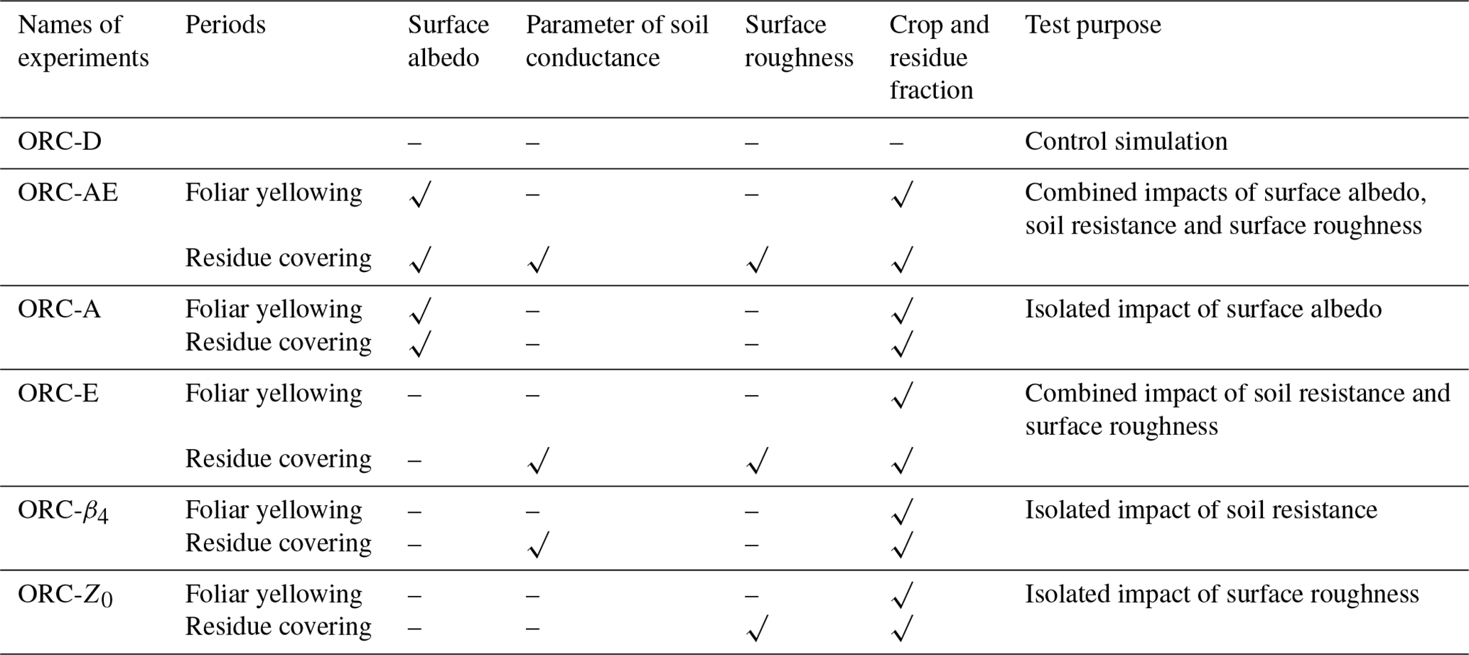
“–” means there is no change, whereas “√” denotes that the corresponding parameter is modified relative to ORC-D. Note that the temporal evolution of foliar and residue albedo, soil resistance parameter, surface roughness, as well as changes in crop and residue fractions, follows the parameterizations described in Sect. 2.3, unless stated otherwise.

2.5 Model simulations

Simulations were performed for 10 sites encompassing 14 farms (Table S2) with the new ORCHIDEE-CROP model version and with the original version of this model (Table 1) for the years for which observations were available. The experiments aimed to evaluate the impacts of the parameterizations of α_surf, β₄ and Z₀ on water–energy cycles during the foliar yellowing and residue covering periods. In the following, ORC-D refers to the default ORCHIDEE-CROP model configuration prior to any modifications, where “D” denotes the default setup. To assess the respective impacts of the five model modifications, we used five different configurations of the improved model. Configuration ORC-AE includes modifications to α_surf, β₄ and Z₀ during foliar yellowing and residue covering periods, where “A” refers to surface albedo and “E” to energy-related parameters. Configuration ORC-A includes only the modified α_surf, while ORC-E incorporates adjustments to both β₄ and Z₀. To further disentangle the individual impacts of β₄ and Z₀, ORC-Z₀ modifies only the Z₀, and ORC-β₄ refers to only the modification of the β₄. The prepared climate forcing data (Sect. 2.1.2), soil texture (sand, silt and clay contents) and crop management information (i.e., sowing date, tillage date, residue covering periods) (Sect. 2.1.3) for each site were used to drive the model. Note that all other management practices prescribed in this model (e.g., nitrogen fertilization) were set as default due to the lack of historical implementation records. There is no irrigation consideration in this analysis.

In addition, we conducted a 10-year simulation (2010–2020) under both current and idealised dry scenarios to quantify the cumulative effects of residue soil cover on water and heat fluxes for the new and old models at six sites if 10-year climate forcing data is available (Table S2). The meteorological forcing data for both scenarios followed the methodology described in Sect. 2.1.2, where the current climate scenario used observed annual climate data from ICOS, and the dry scenario was driven by climate forcing from the driest year (defined as the year with the lowest annual rainfall). The meteorological forcing from the driest year was repeated throughout the simulation period to represent persistent dry conditions. At each site, the sowing and harvesting dates were averaged across the years for which observations were available. The residue covering periods were assumed to persist for 60 d following winter wheat harvest in each year.

2.6 Sensitivity analysis

We performed sensitivity analyses of the major parameters (i.e. k₁, k₄, β₄, H_c, duration of α_surf increase during residue covering period (D_up)) linking to the α_surf variation and the responses of the energy and water budgets, particularly for the ones without enough constraints from field observations. The sensitivity analysis was conducted by changing the parameters by ±10 %, ±20 % and ±30 % from the initial calibrated values. Their impacts of these parameter changes on T_surf, H, E_soil and LE were evaluated.

2.7 Model evaluation

We evaluated the performance of ORCHIDEE-CROP with and without modification against observations of α_surf at site scale. The sites used for evaluation were independent from the ones used for calibration of α_surf.

We computed the coefficient of determination (R²) and RMSE as quality indicators of model performance in the simulation-observation comparison of α_surf during the site calibration and model simulation processes (Wright, 1921; Carbone and Armstrong, 1982):

$$\begin{array}{}\text{(19)}& {\displaystyle }& {\displaystyle }{R}^{\mathrm{2}}=\mathrm{1}-{\displaystyle \frac{{\sum }_i^n(y_i-f_i{)}^{\mathrm{2}}}{{\sum }_i^n(y_i-\underset{\mathrm{¯}}{y}{)}^{\mathrm{2}}}}\text{(20)}& {\displaystyle }& {\displaystyle }\text{RMSE}=\sqrt{{\sum }_i^n{\displaystyle \frac{(f_i-y_i{)}^{\mathrm{2}}}{n}}}\end{array}$$

Where n and i are the number of data and the data i in n in dataset; y_i and f_i are the value of observed data i and the value of fitted data i; $\underset{\mathrm{¯}}{y}$ is the mean of the observed data.

With the calibration of the simulation of harvesting date for all sites, we further compared the simulated surface temperature (T_surf), LE, H from the old and new models against observation during the foliar yellowing and residue covering periods. For each variable, a paired t test was also used to assess the null hypothesis that the mean paired difference between the simulations from the old and new models differed significantly from zero.

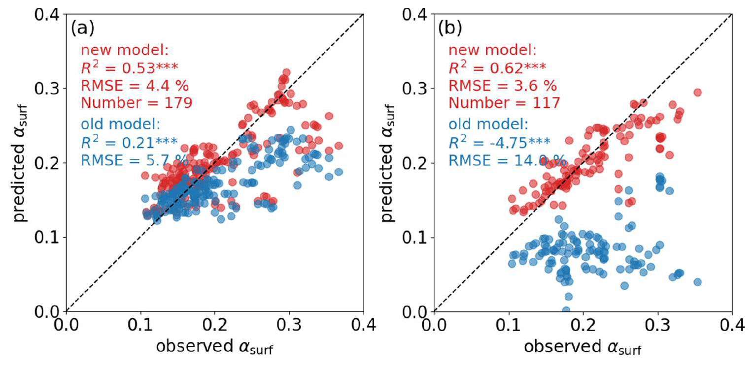
Figure 2 The comparison of daily surface albedo (α_surf) predictions derived from calibration models with and without explicit albedo parameterizations against independent observation from five sites in Europe during (a) the foliar yellowing and (b) residue covering periods. Coefficient of determination (R²) and root mean square error (RMSE) are shown in the upper-left corners of each panel. “${}^{\ast \ast \ast }$” shows the comparison passes the significance level of 0.01. The dotted black line is the 1:1 line.

3 Results

3.1 Evaluation of surface albedo dynamics in the refined ORCHIDEE-CROP model

During the albedo calibration phase, the estimated parameter values of k₁, k₂, k₃ and k₄ (Eqs. 12 and 14) are 0.013 (95 % CI: 0.012–0.013), 1.005 (95 % CI: 0.998–1.017), 0.895 (95 % CI: 0.889–0.902) and 0.0022 (95 % CI: 0.0017–0.0026), respectively. Using these calibrated parameters, the relationship between observed surface albedo (α_surf) and the parameterized α_surf representation used to constrain the model shows a moderate correlation with an R² of 0.54 during the foliar yellowing period and of 0.62 during the residue covering period for five testing sites. The corresponding RMSE values are 0.04 and 0.03, respectively (Fig. 2). The least-squares regression in these two fitting models captures the overall trend in the data better than models that consider them constant, but falls short of reproducing full variation, as it minimizes average errors rather than explaining outliers.

The refined ORCHIDEE-CROP configuration (ORC-AE), represents the new model version incorporating the modified α_surf together with the refined soil conductance (β₄) and surface roughness (Z₀) parameterizations, was used to simulate α_surf dynamics at all 33 site years, which were evaluated independently against observations (Fig. S4a and b in the Supplement). This independent evaluation demonstrates substantially stronger agreement, with significantly higher Pearson correlation coefficients compared to the default model configuration (ORC-D).

ORC-AE captured observed α_surf evolution during the foliar yellowing and residue covering periods across all five sites. Using FR-Gri as an example (Fig. 3), ORC-D without considering their effects on α_surf dynamics shows substantial biases in α_surf during the same period. The results of α_surf at all five sites are presented in Fig. S5 in the Supplement. α_surf increases during spring as crops LAI develops due to the enhanced reflected solar radiation of leaves compared to darker soil followed by a stable period before crops reach maturity. After the crop has reached maturity, the yellowing of aboveground crop biomass increases α_surf. This increase is reversed after harvest as dead and senescent plant material (i.e., residues) starts decomposing. Although the refined model can describe α_surf trends in both foliar yellowing and residue covering periods, substantial biases in α_surf remain for other periods which were not addressed in this study. These discrepancies result from inaccuracies of estimating bare soil albedo (Yu et al., 2026), from the growth of weeds which are not resolved in ORCHIDEE-CROP, and from the simplistic representation of vegetation albedo dynamics before maturity is reached.

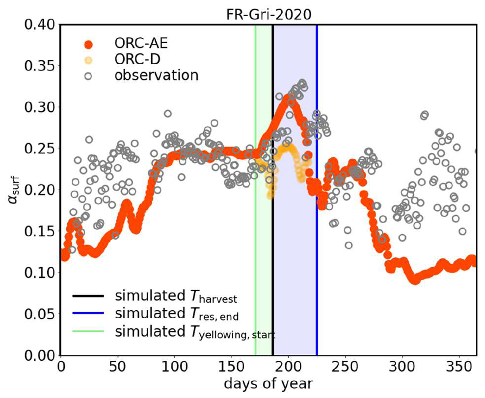
Figure 3 The comparison of surface albedo (α_surf) predicted from the old (orange dots, ORC-AE) and new (red dots, ORC-D) ORCHIDEE-CROP models and observations at Grignon site in France (gray dots) in 2020. ORC-AE represents the new model version with effects of the modified α_surf and the refined soil conductance (β₄) and surface roughness (Z₀), while ORC-D suggests the initial version of the model. The observed α_surf is computed from site radiation measurements through the Integrated Carbon Observation System (ICOS) Data Portal. The green, black and blue solid lines are the simulated start of the foliar yellowing period (shallow green area) (T_{yellowing,start}), harvesting date (T_harvest) and the end of residue covering period (shallow blue area) (T_res,end), respectively.

3.2 The impact of improved surface albedo, surface roughness and soil conductance on soil evaporation, surface temperature and soil water content

Compared with the standard version of ORCHIDEE-CROP (ORC-D), statistically significant changes in averaged surface temperature (T_surf) are detected across sites in ORC-AE and ORC-E (p < 0.05 in t test), resulting from modifications in surface albedo (α_surf), surface roughness (Z₀), and soil conductance (β₄) (Table S5 in the Supplement). In contrast, modifying albedo alone (ORC-A) does not lead to statistically significant changes in soil evaporation (E_soil) during the foliar yellowing period (p > 0.05). Soil water content (SWC) generally does not exhibit statistically significant changes (p > 0.05) in any of the three model configurations. This indicates that, except for SWC, site-averaged differences in the targeted variables are detectable and exhibit consistent signs and magnitudes across sites.

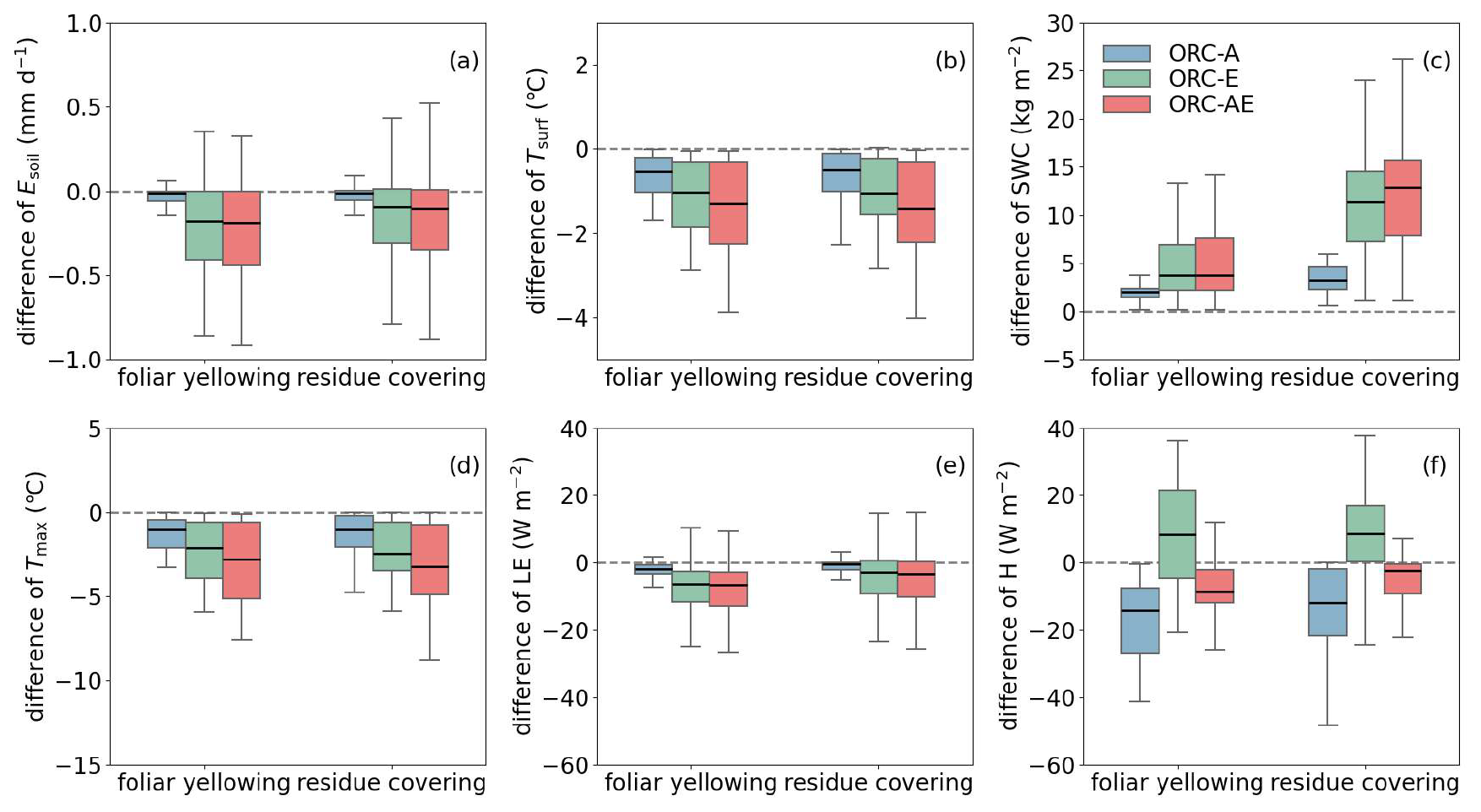
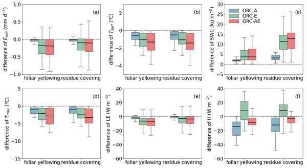
Figure 4 The average effect of model improvements for yellowing and residues cover on daily soil evaporation (E_soil), surface temperature (T_surf), the total soil water content up to 2 m (SWC), the maximum daily surface temperature (T_max), the latent heat flux (LE) and the sensible heat fluxes (H) across 12 sites. Shown are the simulated differences between three configurations of the refined model and old model: ORC-A represents the effect of the modified surface albedo (α_surf), ORC-E shows the effect of refined soil conductance (β₄) and surface roughness (Z₀), and ORC-AE indicates the effect of both modifications. The solid and dotted black lines within each box indicate the mean and median daily values across sites and timepoints, respectively. The box spans the interquartile range, covering the 25th percentile (lower bound) to the 75th percentile (upper bound). Black crossbars at the top and bottom represent the dataset's minimum and maximum values. The grey dotted vertical line in each plot represents zero on the y-axis.

ORC-AE leads to a statistically significant reduction in E_soil relative to ORC-D during foliar yellowing period, with an averaged decrease of −0.18 ± 0.08 mm d⁻¹ (Fig. 4a). A slightly smaller but consistent reduction in E_soil (−0.17 ± 0.14 mm d⁻¹) occurs during the residue covering period. Changes in β₄ and Z₀ (ORC-E) exert significant impacts on E_soil that are comparable in magnitude to those simulated by ORC-AE during both periods, whereas changes in α_surf alone (ORC-A) cause relatively minor and statistically insignificant reductions in E_soil for the same periods. The influence of crop residues on E_soil disappears within approximately 40 d after residue coverage (Figs. S6a and S7a in the Supplement).

The reduced E_soil in ORC-AE leads to a modest but not significant increase in SWC over 2 m soil depth during the residue covering period among all sites (13.30 ± 8.02 kg m⁻²) (Fig. 4c, Table S5). The combined effect is comparable to the sum of the individual contributions from α_surf (ORC-A) and from β₄ and Z₀ (ORC-E), suggesting an approximately additive effect. Although statistically insignificant, this weak water conservation signal persists toward the end of year, with gradual infiltration into deeper soil layers (Fig. S8 in the Supplement).

Incorporating changes in α_surf, β₄ and Z₀ in ORC-AE results in a statistically significant reduction in T_surf during foliar yellowing and residue covering periods with averaged cooling of −1.55 ± 0.93 and −1.90 ± 0.88 °C over all sites, respectively, relative to ORC-D simulation (Fig. 4b). The factorial simulation experiments show that this cooling effect is mainly driven by changes in E_soil and Z₀ (ORC-E), whereas increased α_surf alone produces a weaker and statistically insignificant T_surf reductions. Interaction among α_surf, β₄ and Z₀ (ORC-AE) lead to a dampened overall effect compared with the individual effects of these factors on T_surf. The reduction in T_surf gradually weakened over approximately 60 d as residue cover decreased (Figs. S6d and S7d).

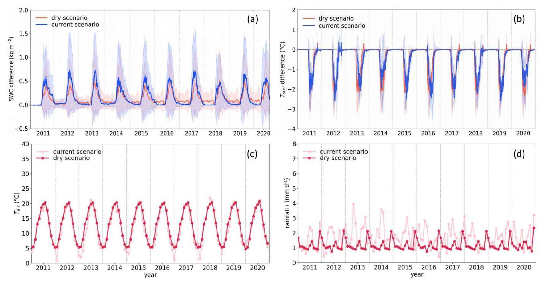
Figure 5 The 10-year cumulated effect of new parameterization of surface albedo (α_surf), surface roughness (Z₀) and soil conductance (β₄) on (a) soil water content (SWC) and (b) simulated daily soil temperature (T_soil) at 12.5 % soil depth under current and dry scenarios at six sites from 2011 to 2020. Monthly temperature and rainfall are obtained from the meteorological variables of 6-hourly 0.5° CRU-JRA product (v2.4), shown in (c) and (d). Shown are differences between results from ORC-AE and ORC-D. ORC-AE represents the new model version with effects of the modified α_surf and the refined β₄ and Z₀, while ORC-D suggests the initial version of the model.

3.3 The impact of improved surface albedo, surface roughness and soil conductance on latent and sensible heat flux

Relative to the ORC-D simulation, statistically significant changes in latent heat fluxes (LE) induced by modifications in surface albedo (α_surf), surface roughness (Z₀), and soil conductance (β₄) are detected across sites for ORC-AE, ORC-A, and ORC-E configurations (p < 0.05 in t test) (Table S5). Changes in sensible heat fluxes (H) are also statistically significant for ORC-AE and ORC-A, whereas modifications in Z₀ and β₄ alone (ORC-E) do not produce statistically significant changes in H (p > 0.05). This suggests that the modified model configurations capture systematic variations in surface water and energy exchanges when averaged across sites.

Modified α_surf, β₄ and Z₀ in ORC-AE leads to statistically significant reductions in LE during the foliar yellowing and residue covering periods, with the changes of −6.84 ± 1.41 and −5.15 ± 4.03 W m⁻², respectively (Fig. 4e). This response is primarily controlled by changes in β₄ and Z₀, represented by comparable reductions in LE by ORC-E. While α_surf alone (ORC-A) plays a more limited role, the effect remains statistically significant. The corresponding changes in the H are also statistically significant and of similar magnitude to the changes in LE induced by the combined effect of α_surf, β₄ and Z₀ during the foliar yellowing and residue covering periods, with averaged decreases of −8.10 ± 4.18 and of −7.44 ± 3.98 W m⁻², compared to the ORC-D simulation (Fig. 4f). In both periods, direct radiative effects associated with increased α_surf (ORC-A) contribute most strongly to the reduction in H, whereas changes in the surface–atmosphere energy exchange (ORC-E) leads only to a slight and statistically insignificant increase in H. Consistent with T_surf response, the influence of crop residues on H weakens over approximately 60 d of residue cover (Figs. S6c and S7c).

3.4 Effect of soil residues on soil water availability on multi-year timescale

The 10-year simulation under current climate shows a minor short-lived increase in SWC at the soil depth of 0.25 m (relative root depth of winter wheat in ORCHIDEE-CROP model) due to the presence of crop residues. Averaged across the simulation period and the six sites, total SWC is 0.24 ± 0.60 kg m⁻² (2.81 ± 6.15 %) higher than in the simulation without crop residues (Fig. 5a). No clear carry-over effect of SWC retention from one growing season to the next is observed at any site. This occurs because increased drainage losses compensated for reduced bare soil evaporation (Fig. S9 in the Supplement). Soil temperature (T_soil) at 0.25 m soil depth penetrable by winter wheat roots decreased by an average of −0.37 ± 0.77 °C (7.56 ± 5.96 %) over the 60 d of residue covering periods across sites, with no consistent temporal evolution during the 60 d residue covering periods over 10 years (Fig. 5b). The largest reduction in T_soil occurs shortly after harvest, coinciding with the largest increase in α_surf due to residue presence compared to simulation without residue effects.

In the dry scenario, the meteorological forcing corresponds to a single dry year that is repeatedly applied over the 10-year simulation. This idealized experiment is designed to explore the sustained response of the system under persistent dry conditions, rather than to represent future climatic conditions or interannual climate variability.

Under these conditions, the presence of crop residue shows a similar increase in SWC at 0.25 m soil depth under current climate, with an average increase of 0.23 ± 0.53 kg m⁻² (3.01 ± 5.97 %) compared to simulations without residues (Fig. 5a).

Although no systematic temporal evolution is observed in near-surface SWC (at the soil depth of 0.25 m), deeper soil layers (50 % soil depth) exhibit a slight gradual increase of soil moisture over the simulation period (not shown) due to the sustained reduced E_soil which increases downward water transport. The decrease in E_soil by crop residues allows more water to remain in the soil, leaving more residual moisture available for the next growing season.

Average T_soil at 0.25 m soil depth decreases with a statistically significant trend by an average of −0.42 ± 0.80 °C (−8.42 ± 3.58 %) over years (Fig. 5b), consistent with the sustained effects of residue-induced surface cooling.

3.5 Sensitivity of energy and water processes to parameters

Sensitivity analyses reveal pronounced nonlinear responses of land surface water and energy processes to variations in model parameters (Fig. S10 in the Supplement). For T_surf, k₁ exhibits the highest sensitivity, as it governs both the rate and maximum magnitude of the 15 d in surface albedo and consequently modulates available surface radiation during the residue covering period (Fig. S10a). A ±30 % perturbation in k₁ induces 8.69 % and 30.78 % enhancements in surface cooling, respectively. This reflects a nonlinear response, as k₁ controls not only the rate of albedo increase but also the initial value of the subsequent decay phase (Sect. 2.3.2). Combined with the gradual decline in residue fraction over time, changes in k₁ modify the cumulative contribution of residue albedo to surface radiation, leading to enhanced cooling in both cases. In contrast, T_surf is only weakly affected by the hydrological parameter β₄ (−4.46 %$/+$2.98 % change in surface cooling for ± 30 % variations), consistent with the scenario simulations (Fig. 4b). The parameter D_up also exerts only a limited influence on T_surf (−8.35 %$/+$2.53 % change in cooling for ± 30 % variations).

For E_soil, β₄ is the dominant control (Fig. S10b). A decrease or increase in β₄ from the baseline by 30 % results in a 62.48 % reduction or 100.85 % increase in the decline of E_soil, respectively. The parameters k₁, k₄, and D_up also influence E_soil, with a ±30 % variation leading to −32.40 %$/-$35.53 %, −17.72 %$/+$22.35 %, and −29.49 %$/-$18.57 % changes, respectively.

For H, D_up exerts the strongest control, followed by k₁ and β₄ (Fig. S10c). Adjusting these parameters by ± 30 % alters H by −10.53 %$/+$56.34 %, −42.55 %$/+$36.77 %, and −27.60 %$/+$27.33 %, respectively. β₄ is also the most sensitive parameter controlling LE, reflecting the dependence of LE on E_soil. ±30 % variations in β₄ yield +89.78 %$/-$62.16 % changes in LE (Fig. S10d). In contrast, the strong sensitivity of E_soil to k₁ does not propagate to LE, with only −2.66 %$/+$8.21 % changes observed under equivalent k₁ perturbations (Fig. S10c and d).

4 Discussion

4.1 Surface energy and land–atmosphere interaction jointly regulate surface temperature during foliar yellowing and residue covering periods

Foliar yellowing and residue coverage cool the surface across all sites by regulating the surface energy balance and redistributing net radiation to latent and sensible energy fluxes (Fig. 4a). Compared with the initial expectation that would dominate the impact of α_surf, the larger surface temperature (T_surf) decrease in ORC-E than that in ORC-A reveals that the cooling from the surface–atmosphere water–heat exchange due to modified soil conductance (β₄) and surface roughness (Z₀) drives the change in T_surf. Previous work indicated that no-tillage systems with residue coverage at the European scale cooled the surface by approximately 2 °C during hot summer days due to increased α_surf (Davin et al., 2014). Our simulations at site scale further highlight that the local changes in turbulent processes can exert a comparable control over T_surf, relying on different spatial scales, climate conditions, phenological stages and surface properties (McDermid et al., 2019).

While foliar yellowing and residue coverage induce an albedo-driven redistribution of surface energy budget across all 10 European sites, the interplay between available surface energy and the surface–atmosphere water–heat exchange causes substantial variation in the magnitude and duration of cooling. The increased Z₀ during winter wheat growth and residue covering periods enhances surface–atmosphere turbulent heat exchange, potentially promoting more efficient heat dissipation and surface cooling (Winckler et al., 2019; Meier et al., 2022). For example, when isolating the impact of increased Z₀ due to foliar yellowing and residue coverage (ORC-Z₀), both contribute more to the cooling impact than ORC-β₄ across all sites (Fig. S11a in the Supplement). However, the persistence of this surface cooling also depends on the hydrological fluxes between surface and atmosphere. Crop residues potentially warm the surface by decreasing soil evaporation (E_soil) (Hu et al., 2018). This effect can occur through reductions in β₄ caused by shielding the soil from direct solar radiation and wind (Fig. S11a), and by reducing near-surface wind speed and enhancing aerodynamic drag via increasing Z₀ (Figs. 4a and S11b). Similar to residue coverage, foliar yellowing has a comparable influence on E_soil due to the continuous coverage provided by winter wheat (Fig. 4a). The associated decline in transpiration, driven by reduced stomatal conductance under lower net radiation, may contribute to surface warming (not shown). Residue-induced suppression of E_soil during the residue covering period and radiation-induced decline in transpiration during foliar yellowing, both redirect energy partitioning from latent heat flux (LE) towards sensible heat flux (H), likely offsetting surface cooling (Fig. 4f) (Ramos et al., 2024).

4.2 Distinct controls on LE and H during foliar yellowing and residue covering periods

To isolate the drivers of turbulent flux changes during crop yellowing and residue cover periods, we analyzed results from two key model configurations: the surface–atmosphere interaction experiments (ORC-E) and the radiative forcing experiments (ORC-A). Our simulations revealed that the surface–atmosphere interactions (ORC-E) dominate the reduction in LE during both periods (Figs. 4e and S6b), with this effect jointly mediated by changes in β₄ and Z₀ (Fig. S11d), while α_surf-driven radiative impact is less important. In contrast, the reduced availability of surface energy with a higher albedo during crop yellowing and the residue cover period, together with the subsequently altered turbulent fluxes, contributed to a modest reduction in H during these periods due to their opposing effects (Figs. 4f and S6c). During this process, the enhanced H is primarily mediated by Z₀ (Fig. S11c).

The different underlying drivers behind changes in LE and H can be explained by the following: LE represents the energy needed for water vaporization and is therefore constrained by available energy and moisture transport efficiency (Chen et al., 2024). In contrast, H is driven by direct surface–atmosphere heat transfer via conduction and convection, governed by the land-air temperature gradient and turbulent heat exchange (Myhre et al., 2018). For example, we found that during the residue covering period, changes in β₄ and Z₀ (ORC-E) tend to increase H, while the albedo-induced reduction in net radiation (ORC-A) acts in the opposite direction by limiting the available energy for sensible heating (Fig. 4f). These results highlight that changes in LE and H are not controlled by a single mechanism but emerge from the combined and counteracting effects of radiative forcing and surface–atmosphere coupling. This finding is consistent with earlier findings pointing to a critical role of surface–atmosphere interactions in shaping energy partitioning and near-surface thermal dynamics (Koster et al., 2004; Seneviratne et al., 2010; Dare-Idowu et al., 2021; Denissen et al., 2022; Hsu and Dirmeyer, 2023).

The individual impacts of α_surf (ORC-A) and surface–atmosphere exchange (ORC-E) on the changes in LE and H differ from their combined effect of both (ORC-AE), especially during the residue covering period (Fig. 4). This indicates a strong nonlinear interaction between energy and water dynamics driven by crop residues (Hsu and Dirmeyer, 2021). For example, the decreased LE reduces H during the residue covering period by weakening near-surface turbulence, thereby producing a residual negative impact on H that could not be explained by ORC-A and ORC-E individually (Fig. 4f, Table S5). The complex feedback mechanisms between radiation partitioning and surface–atmosphere coupling require modelling approaches which take into account both interactions (Hsu and Dirmeyer, 2021, 2022).

It should be noted that in both periods, the averaged difference in surface energy fluxes (i.e. LE and H) between the new and old models across all sites are generally modest (Fig. 4e and f) and are of similar magnitudes to the model uncertainty (Table S5), which masks a substantial spatiotemporal variability in the effects of yellowed leaves and covered residues. Temporally, residue-induced albedo enhancement peaks within the first 15 d after harvest and weakens as residues decompose, causing short-lived but locally significant perturbations in water and heat fluxes (Figs. 3, S5 and S6). The residue impact on the water–heat processes persists for approximately one additional month after residue removal through tillage or natural decomposition (Fig. S7). Spatial variations in climate, soil properties, and management practices amplify local differences in residue effects. For example, we found that during the residue covering period, BE-Lon exhibits the largest mean relative decrease in LE in the new model compared to the old model (−27.42 ± 26.20 %), whereas the change at DE-Geb is minimal (5.73 ± 64.90 %). This contrast arises because the higher soil moisture and sandy texture at BE-Lon support greater evaporative fluxes, whereas the limited soil water and clay-rich soil at DE-Geb favor energy dissipation as sensible rather than latent heat (Dumont et al., 2024; Buysse et al., 2023). In addition, long-term simulations show the accumulated residue impact on heat budgets. The 10-year simulation under the dry scenario shows a low but statistically significant cooling trend, with a yearly average of −0.3 °C (Fig. 5). This demonstrates that even modest instantaneous flux changes can produce meaningful long-term surface cooling effects.

4.3 Implication for climate change mitigation and adaptation

With approximately 60 % of global croplands having higher T_surf than surrounding natural biome types, elevated temperatures, particularly during extreme heat and drought events, pose a major issue for crop yields and food security (Lobell et al., 2012; Hatfield and Prueger, 2015; Lesk et al., 2022; Chen et al., 2024). Our simulations across all sites suggest that residue coverage alleviates heat stress by significantly decreasing maximum surface temperature (T_max) during approximately 30 d residue covering period and for up to 50 d afterward (Figs. S6e and S7e). This result aligns with previous findings on the cooling effect of crop residues (Davin et al., 2014; Webber et al., 2018; Su et al., 2021). Reduced surface T_max after crop harvest mitigates heat stress on soil biota, providing a more favorable growing environment for subsequent crop cycles (Hatfield et al., 2015). Sustained temperatures above 30 °C can stress mesophilic soil microbes, inhibiting decomposition and nutrient cycling (Pietikäinen et al., 2005). Our simulations show that residue cover reduces T_max beyond 30 °C on 26 % of days during the residue period and 3.8 % of days afterward, underscoring its role in regulating soil thermal condition. This buffering effect modifies microbial activity and soil organic matter decomposition rates depending on local climatic and environmental conditions, thereby influencing greenhouse gas emissions from soil respiration (Knight et al., 2024).

The increase in H during residue covering period reveals an increased surface-air temperature gradient caused by reduced T_surf, possibly leading to warming of the lower atmosphere which cannot be quantified by the land surface model only (Figs. 4, S6c, and S7c). This shift in energy partitioning from LE to H, driven by reduced E_soil due to residue coverage, might mitigate surface warming while potentially intensifying regional heat stress. Consequently, it introduces uncertainty regarding the effectiveness of crop residues as a climate mitigation strategy. Notably, the use of fixed air temperature forcing data partially explains the increase in H because the constant air temperature ignores atmospheric feedback (Luyssaert et al., 2014). As a result, the climate mitigation potential of residue management remains uncertain, and its regional impact on energy partitioning cannot be fully quantified. It is essential to consider not only surface cooling but also changes in air temperature, as the latter is more directly linked to climate dynamics. A coupled simulation, feasible with ORCHIDEE-CROP, would be needed for future studies.

Soil water content (SWC) dynamics play a key role in regulating the land–atmosphere interactions, as the increase in surface soil SWC, as due to residue effects on roughness and soil resistance, can decrease H partitioning via promoting E_soil (Myhre et al., 2018). The 10-year simulations further highlight that residue coverage has the potential to increase SWC and thereby mitigate drought stress, particularly under drier conditions with fewer rainfall events (Figs. 5 and S9). In such condition, SWC remains high within the upper 1 m soil for extended periods of up to 3 months. An earlier review suggested that dry soil condition might result in soil compaction and reduced hydraulic conductivity (Singh et al., 2018). This limits infiltration and slow downward water percolation, which might hinder the underlying mechanism responsible for upper-soil SWC retention simulated by the ORCHIDEE-CROP model. Notably, soil texture modulates this effect. For example, rapid water infiltration into deeper layers in sandy soils with high drainage reduces surface SWC availability for cooling and plant uptake (Fatichi et al., 2020; Wankmüller et al., 2024), highlighting how soil hydraulics constrain residue efficacy. The sustained SWC also fosters soil biota activity (e.g., fungi, earthworms), which enhance soil structure through aggregate formation and organic matter decomposition (Li et al., 2009). Improved soil structure increases water-holding capacity, creating a positive feedback loop where residue-induced SWC retention supports biological activity, which in turn amplifies long-term moisture retention. This synergy reveals that residue effects on SWC persist beyond immediate rainfall events, particularly in water-limited systems.

External factors such as tillage timing and precipitation frequency also affect the biophysical impacts of crop residues (Konapala et al., 2020). Early tillage, as observed at the FR-Gri site in 2018 (3 weeks after harvest), retains more SWC in the topsoil and removes the residue cover, thereby temporarily enhancing E_soil and LE after the end of residue covering (Fig. S12 in the Supplement). The strong soil water retention capacity of the silt–loam soil at this site further contributed to this effect (Houot et al., 2000). This process underscores the importance of management practices in regulating the diverse hydrological and thermal effects of residue covering. Targeted strategies are also essential for optimising water use, particularly facing warmer and drier climates (Swain et al., 2025).

4.4 Uncertainty and Limitations

Despite improvements to the ORCHIDEE-CROP model in simulating crop albedo changes associated with foliar yellowing and crop residues, as well as their biophysical climate impacts, uncertainties and limitations remain.

α_surf shows the most consistent improvement across sites, reflecting its direct control by the new parameterizations for foliar yellowing and residue covering (Figs. 2 and S4a, b). However, degraded performance is observed at two sites (DE-Geb in 2014 and FR-Aur in 2019; Fig. S5a and c). At these sites, the refined configuration simulates higher α_surf during foliar yellowing and residue covering than those estimated from site radiometer measurements. Surface conditions shown by the site photos suggest that the discrepancy may be related to limitations in the spatial representativeness of point-scale observations, which is further investigated in Sect. S1.2 in the Supplement. T_surf also improves significantly, especially during the foliar yellowing period (Fig. S4c and d). In contrast, LE and H exhibit moderate improvement during the residue covering period and little to no improvement during the crop growth and foliar yellowing periods (Fig. S4e–g). This performance is expected, as LE and H during the growing season are primarily governed by transpiration processes that are not recalibrated in this study. During the residue covering period, remaining biases in LE and H likely arise from unrepresented processes associated with residue cover, such as water interception and retention by residues and soil hydraulic heterogeneity. Limitation in the representation of land–atmosphere coupling in ORCHIDEE also contributes to persistent uncertainties in simulated turbulent fluxes (Sect. 4.3).

The ORCHIDEE-CROP model exhibits biases in simulating water and energy fluxes, and the performance of the new model in reproducing water–energy fluxes does not improve relative to the previous version when evaluated against site-level measurements at six sites (Fig. S4). Both the new and old models overestimate LE and H during foliar yellowing periods, while underestimating LE and overestimating H during residue covering periods. This overestimation during foliar yellowing periods might come from excessively strong vegetation–atmosphere coupling for crops within ORCHIDEE itself compared with observation (Zhang et al., 2022c). Observations indicate that LE is higher during periods with residue coverage than during periods of bare soil exposure (Fig. S13 in the Supplement). However, it remains unclear to what extent the observed difference in LE is driven by differences in weather conditions rather than by the presence or absence of residues. One possible source of bias during the residue covering period may be the simplification of model parameters. In the present version of ORCHIDEE-CROP, the effects of crop residues on surface–atmosphere coupling are quantified by modulating β₄ and Z₀. Both variables are represented using uniform assumptions to balance model complexity against the scarcity of data available for parameterization. Specifically, the impact of residues on β₄ was represented using an initial reduction factor of 0.5 at the beginning of the residue covering (Sect. 2.3.3). The residue influence on Z₀ was prescribed using a fixed residue height (0.5 m), derived from the average of measurements across five winter-wheat sites (Sect. 2.3.4, Table S3). These parameter choices are applied uniformly across all sites and therefore cannot explicitly represent local variation in residue characteristics, soil properties, atmospheric conditions and management practices. As a result, the model is incapable of fully resolving site-specific residue impacts, which potentially contributes to the bias of simulated LE and H at certain sites.

The sensitivity analysis also highlights the uncertainties associated with parameter selection (Fig. S10). The β₄ and k₁ exert strong control over the spatiotemporal partitioning of available energy between LE and H. The use of fixed parameter values and limited calibration based on only a few sites inevitably contributes to model uncertainty and constrains the representation of local variability.

We manually adjusted the total conductance associated with soil evaporation, transpiration and interception in ORCHIDEE-CROP by scaling it with 1+f_soil during residue cover periods (Chapin et al., 2011). The simulations showed improved agreement with observed T_surf, LE and H (Fig. S14 in the Supplement), indicating that the net biophysical impact of residue cover enhanced surface–atmosphere water and heat exchanges despite inhibiting soil evaporation, which is not well described in the current model. A test of quantifying the residue impact on E_soil at 15 field experiments distributed globally showed that residue cover exceeding 80 % resulted in an approximately 20 %–30 % reduction in E_soil during the residue covering period (not shown). Therefore, the assumed 50 % initial decline in β₄ in the improved model (Eq. 16) might overestimate residue impacts, potentially explaining the lower E_soil and LE simulated across sites in the new model compared with both the initial model version and observations (Fig. S4).

While our modelling shows minor effects of crop residues on SWC, we did not account for effects such as changes in soil texture or organic matter content (Singh et al., 2018), which could improve soil water availability to crops. In addition, we did not account for interactions with other managements such as tillage, which are often co-applied. In summary, the present simulations are particularly well suited for assessing the biophysical impacts of residue cover on the surface energy balance, while the representation of soil–water responses remains an area requiring further model development and the corresponding results should therefore be considered with caution.

For example, specific hydrological processes impacted by crop residues were not accounted for in this study, such as water interception on the surface of residues, and uptake or release of water by residues (Kozak et al., 2007, Swella et al., 2015). Rainfall interception by residues alters both the timing and magnitude of soil–water inputs and enhances evaporation from residue surfaces, thereby modifying surface moisture conditions and heat exchange processes (Mitchell et al., 2012; Thapa et al., 2021). However, contrasting evaporation mechanisms operating in soil and residue layers introduce additional complexity into surface evaporation processes. The omission of these processes likely increases model uncertainty in biophysical simulations under variable rainfall conditions.

The input data used to drive the model introduces several structural uncertainties. First, while site-based meteorological forcing (e.g., air temperature, wind speed, humidity) provides high representativeness, meteorological observations and direct radiation measurements were unavailable at two ClieNFarm sites comprising six farms (UK-Rookery, UK-Winwick, UK-Allerton, BE-AH, BE-BM, and BE-LB; Table S2). For these sites, simulations were instead driven by the hourly 0.25° ERA-interim product and surface albedo was derived from Sentinel-2 observations. This substitution inevitably limits the ability of our model to reproduce site-specific water and energy dynamics. A comparison between satellite-derived albedo at 300 m spatial resolution and albedo calculated from shortwave radiation measurements representing only a few m² at eight sites reveals systematic differences (Fig. S15 in the Supplement). These differences are likely attributable to spatial scale mismatch, cloud screening effects, and surface heterogeneity, which together dampen albedo variability in the satellite product. While satellite-based albedo enables the inclusion of these six field sites, the substituted values introduce additional uncertainty in the simulated surface energy fluxes. Second, the bare soil albedo dataset used to estimate surface albedo carries uncertainties related to quality-restricted training samples (Yu et al., 2026). For example, the vegetation index thresholding used to identify bare soil may also include mixed surfaces containing crop residues, introducing biases into soil albedo retrievals. Also, the spatial aggregation from 300 m to 0.5° smoothes the field variability of bare soil albedo, reducing the reliability of the model simulation. Third, the incomplete representation of management practices in our model, including fertilizer and pesticide application as well as physical operations such as tillage, limits the model's capacity to reproduce observed variations in crop phenology, soil water content, and surface fluxes across years.

Based on these concerns, evaluating residue effects requires a context-specific approach that accounts for the interactions among climate, soil, and crop characteristics. Process-based land surface models provide an effective framework for such assessments across multiple scales, as they explicitly represent the coupled biophysical and ecological mechanisms controlling surface energy and water exchanges. This approach provides opportunities to guide residue management strategies under diverse environmental settings. Future model developments should incorporate explicit residue modules and site-specific parameterization to better capture spatial heterogeneity in residue impacts on energy and water fluxes. For example, integrating the canopy interception modules developed by crop models to ORCHIDEE-CROP is a good strategy to better represent the residue impact on the hydrological dynamics, such as CropSyst and RZWQM (Kozak et al., 2007). Moreover, an open-sourced global database derived from dedicated field trials monitoring energy exchange is required for parametrizing and evaluating these model developments.

5 Conclusion

In this study, we improved the simulation of winter wheat cultivar in the ORCHIDEE-CROP model by taking into account the impact of foliar yellowing and crop residues on water and energy balance of winter wheat cultivations based on observations from 10 cropland sites. The simulated surface energy budget and partitioning of latent and sensible heat fluxes show a cooling impact of residues and crop yellowing. A complex interplay between radiative and turbulent processes controls the strength of these effects. The improved ORCHIDEE-CROP model, which includes representations of land surface albedo, surface roughness, and soil conductance for residue covering, provides a valuable tool for quantifying biophysical impacts and guiding localized residue management strategies from regional to global scales. Future model developments should refine the representation of crop residue effects on soil physio–chemical properties and interactions with management practices such as tillage in order to improve simulations of plant water availability. By identifying optimal residue management practices, this approach can contribute to sustainable agriculture and support policy development in the context of climate warming.