DReaMIT: a dynamical reanalysis framework for modelling surface-based temperature inversions in cold environments

Surface-based temperature inversions (SBIs) are critical to high-latitude mountain climatology, shaping permafrost stability and near-surface thermal regimes. This study develops and evaluates a new surface-based inversion model, DReaMIT (Dynamical Reanalysis Model for Inversions of Temperature), that extends the framework of Pozsgay and Gruber (2025) by spatializing the inversion strength parameter (α) using hypsometric position rather than absolute elevation. The reformulated approach enables a unified calibration across two contrasting Yukon valleys (WS01 and WS02), improving model transferability and reducing site-specific bias. The model also goes beyond the linear treatment of the hypsometric variable to capture the observed nonlinear decay of lapse rates within SBIs, consistent with in-valley observations where temperature increases of up to 8 °C over 19 m were recorded. Model performance was assessed across the Yukon and Northwest Territories, where it successfully reproduced inversion structure even in areas with weaker or transient SBIs, such as Whitehorse and Haines Junction. Limitations were observed in flat regions with minimal hypsometric relief (e.g. Tulita, Old Crow), highlighting cases where microtopographic indices may better represent cold-air pooling potential. The new hypsometric formulation enhances the physical realism and spatial applicability of SBI modelling, providing an empirically-constrained, transferable tool for predicting near-surface temperature regimes and assessing permafrost sensitivity under northern climate change.

1 Introduction

Observational climate data are sparse and discontinuous in high-latitude (Urban et al., 2013; Way and Bonnaventure, 2015) and alpine regions (Oyler et al., 2015; Pepin et al., 2022). In contrast, climate reanalysis products provide spatially- and temporally-consistent datasets that extend back more than 75 years, since 1940 for ERA5 (fifth-generation ECMWF atmospheric reanalysis of the global climate) (Hersbach et al., 2020) and 1948 for JRA-3Q (Japanese Reanalysis for Three Quarters of a Century) (Hersbach et al., 2020; Kosaka et al., 2024). These datasets are improving through updates to their modelling and forecasting systems, resulting in comprehensive coverage of surface and atmospheric conditions at multiple atmospheric pressure levels. Consequently, reanalysis products are a valuable resource in areas that have sparse observational data and are used to inform modelling, such as predictions of permafrost (e.g. Liu et al., 2025; Obu et al., 2019; Tao et al., 2019; Fiddes et al., 2015) and hydrological processes (e.g. Nkiaka et al., 2017; Tarek et al., 2020).

However, the coarse spatial resolution of reanalysis products (tens of kilometers) limits their applicability in mountainous terrain, where complex topography can produce climate variations comparable to those observed across thousands of kilometers in latitude (Riseborough et al., 2008). This sub-grid heterogeneity, and the local processes it drives, are not captured by coarse resolution (Etzelmüller, 2013).

To address this limitation, a variety of downscaling methods have been developed to scale coarse resolution climate reanalysis data to finer resolutions or scale-free point locations (e.g. Draeger et al., 2024; Ntagkounakis et al., 2023; Wang et al., 2016; Zhang et al., 2020). Among these, TopoSCALE (Fiddes and Gruber, 2014) and TopoCLIM (Fiddes et al., 2022) use topography-based parameterizations to reproduce small-scale variability, while Globsim (Cao et al., 2019) extends these methods by integrating multiple reanalysis datasets to generate meteorological time series for specific sites. These models have been shown to effectively predict weather conditions with limited bias; however, residual errors remain in regions where complex local processes are not resolved in the reanalysis model (Daly et al., 2008; Roberts et al., 2019). Furthermore, reanalysis data can have regional or temporal trends in bias, especially given that they are less reliable for earlier periods (Urraca and Gobron, 2023).

SBIs remain a major source of uncertainty in reanalysis models. In layman terms, SBIs are weather events where the air temperature increases with elevation, in opposition to the expected behaviour, and leading to a stratified air column with cold and dense air trapped in valley bottoms below warmer layers. In high-latitude mountains, near-surface temperatures are often influenced by surface-based inversions. These conditions are poorly represented by conventional lapse-rate-based downscaling approaches and coarse-resolution reanalysis products, leading to systematic biases in reconstructed surface temperatures. The longer, deeper, and intense these inversions are, the more important a model becomes to efficiently take them into account in reconstructing the near-surface air temperatures, with downstream applications such as permafrost modelling, hydrology, and infrastructure-relevant thermal regimes. Thus, improving the representation of SBIs in reanalysis-derived products can have practical applications for non-specialist users beyond the model development itself.

To reduce these biases, Pozsgay and Gruber (2025) developed a model that explicitly accounts for the influence of surface-based temperature inversions (SBIs) on near-surface air temperature and that includes a temporal bias correction parameter. This model dynamically corrects downscaled reanalysis data at hourly time steps, improving the representation of near-surface temperatures under stable atmospheric conditions. This is done by incorporating a conceptual framework introduced by Noad et al. (2023), which defines SBI magnitude as the strength of an SBI (temperature increase from the bottom to the top of the SBI) added to the expected surface air temperature if the lapse rate above the SBI layer were to continue to the surface.

This approach addresses a key limitation in downscaling methods, an assumption that the lapse rates are normal below reanalysis grid elevation, i.e. extrapolated temperatures from lowest atmospheric levels and a smooth vertical gradient, disregarding intense SBIs at these low elevations. In subarctic valleys, prolonged periods of nocturnal radiative cooling during the winter promote deep, intense, and long-lasting SBI events (Fochesatto et al., 2015; Mayfield and Fochesatto, 2013; Noad and Bonnaventure, 2022, 2024). These SBIs generate strongly positive mean annual lapse rates (upwards to 25 °C km⁻¹) within the first 100–150 m above the valley floor (Noad and Bonnaventure, 2026), leading to substantial biases when unresolved below the grid level of the reanalysis product.

Initial testing of the Pozsgay and Gruber (2025) model using a dense network of air temperature sensors across two subarctic valleys demonstrated that the model performs well when calibrated locally, but suffers from a lack of transferability. In this study, we aim to enhance the generalizability of the Pozsgay and Gruber (2025) inversion correction model by testing new parameters beyond the original use of absolute elevation. Specifically, we evaluate additional topographic variables (e.g. relative elevation and hypsometry) to better represent the influence of local terrain on cold-air pooling and SBI dynamics. By calibrating these parameters across multiple valleys and testing them at other locations in northwestern Canada, we will identify the optimal parameters and functional form of the model to increase prediction performance regionally, without requiring additional local calibration. This work contributes to the improved use of reanalysis in their ability to represent sub-grid processes in complex terrain. The resulting model parameterization will increase their reliability for important applications such as permafrost or hydrological modelling.

2 Study area

2.1 Dempster

The study area of this paper consists of two northcentral Yukon valleys, approximately 120 km to the north-east of Dawson City, around Distincta Peak (1790 m a.s.l.), the dominant point in the subrange of mountains. These valleys will be referred to as WS01 and WS02 (for weather station 1 and 2), and correspond to valleys labelled as SVWS and NVWS, respectively, in Noad and Bonnaventure (2022). Those sites are easily accessible by road, being located in the immediate vicinity of the Dempster Highway. They were shown to be prone to intense, frequent, and long-lasting inversion events (Noad and Bonnaventure, 2022, 2026).

The two valley floors are separated by approximately 8 km, with WS01 to the south of Distincta Peak, and WS02 to the north. The former is an approximately 5.5 km-long V-shaped valley, with elevations ranging from 950 m at the outlet and 1700 m on the closest highest ridge. The latter is an approximately 6.5 km-long U-shaped valley, with elevations comprised between 1040–1790 m. The valleys' outlet is oriented towards the southeast for WS01, and to the north for WS02.

The network of air temperature loggers consists of 24 locations in valley WS01, and 26 in WS02. The locations are chosen to sample the widest range of elevation, slope, aspect angle, and degree of valleyness (Cao et al., 2017).

2.2 Dawson

The model calibration of this paper will be tested on the dataset presented in Pozsgay and Gruber (2025), where five weather stations are distributed within a 25 km radius from the Dawson airport, and with elevations ranging from 370 to 1200 m.

2.3 ECCC/NAVCAN weather stations

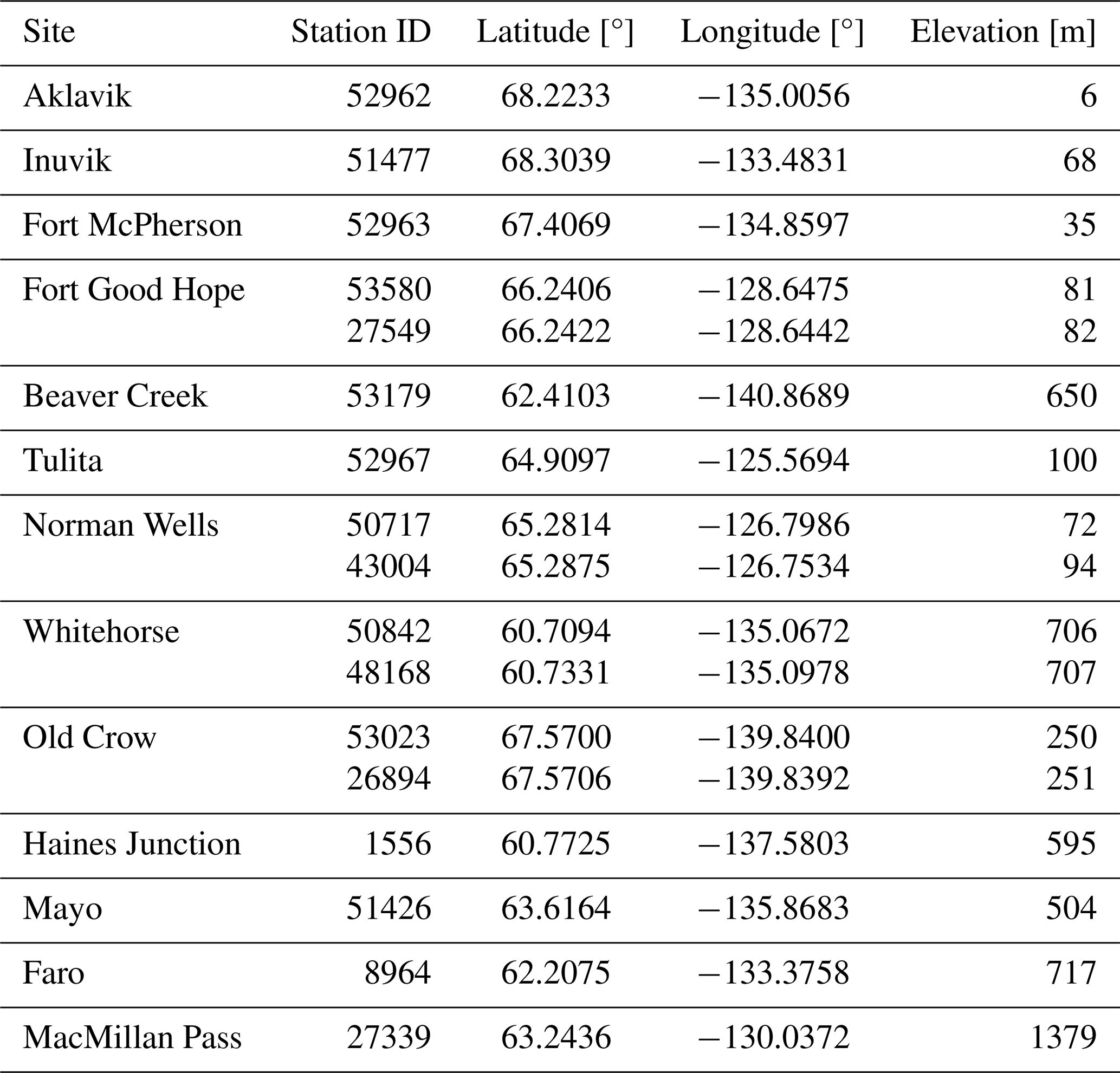
Finally, the temperature inversion model will also be applied to various sites across northern Canada, in the Yukon and Northwest Territories. We selected 13 ECCC/NAVCAN weather stations (Fig. 1, see Table E1 for coordinates) because they span a wide spatial area and a variety of topographic conditions, from river delta to mountainous terrain.

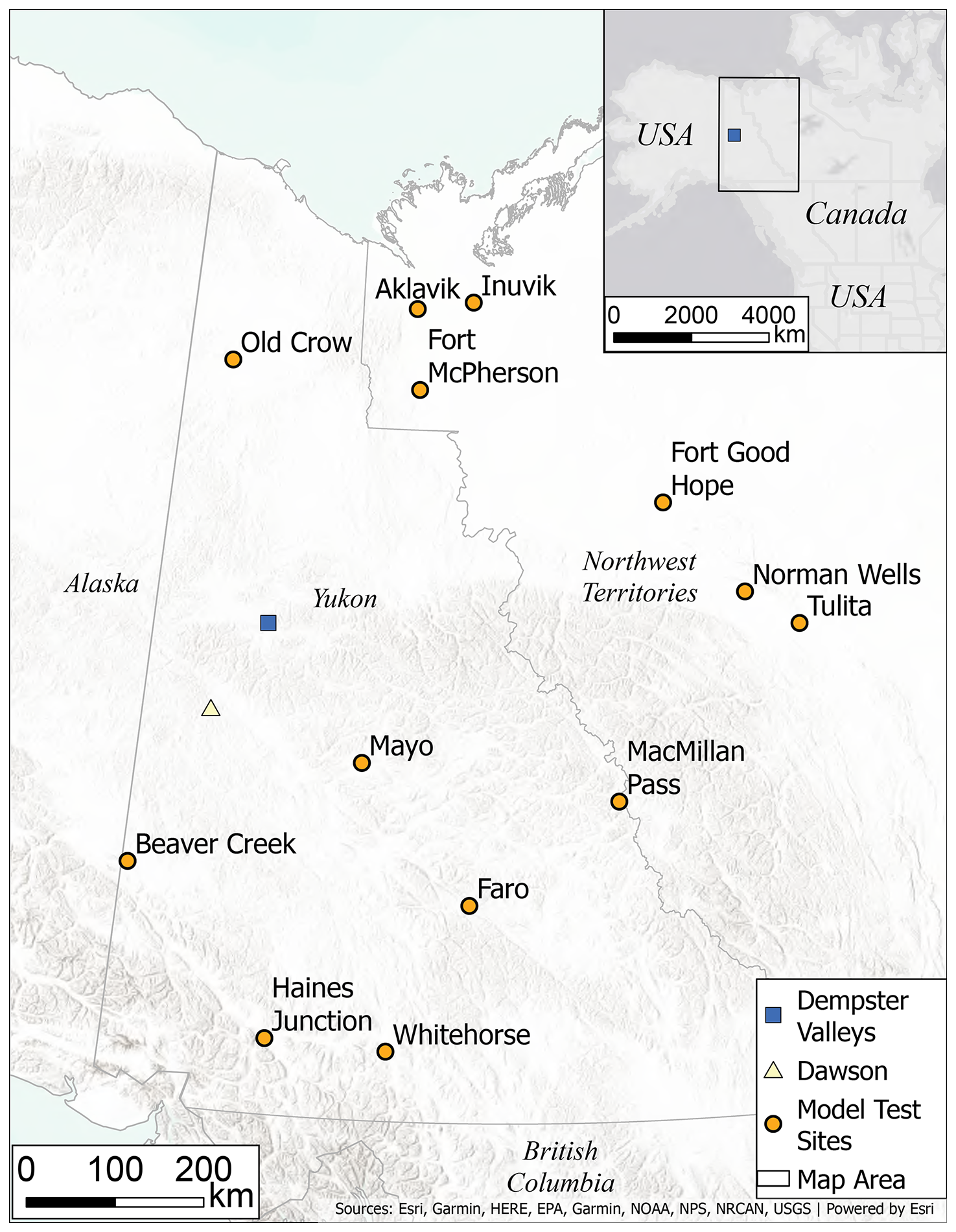
Figure 1 The Dempster study valleys (blue point), Dawson City (yellow point), and 13 Environment Climate Change Canada (ECCC) and Navigation Canada (NAVCAN) weather station locations (orange points) situated across Yukon and Northwest Territories.

Then, we report the distribution of elevations in a radius of 50 km around each station in Fig. 2, together with all sites from the Dempster and Dawson areas.

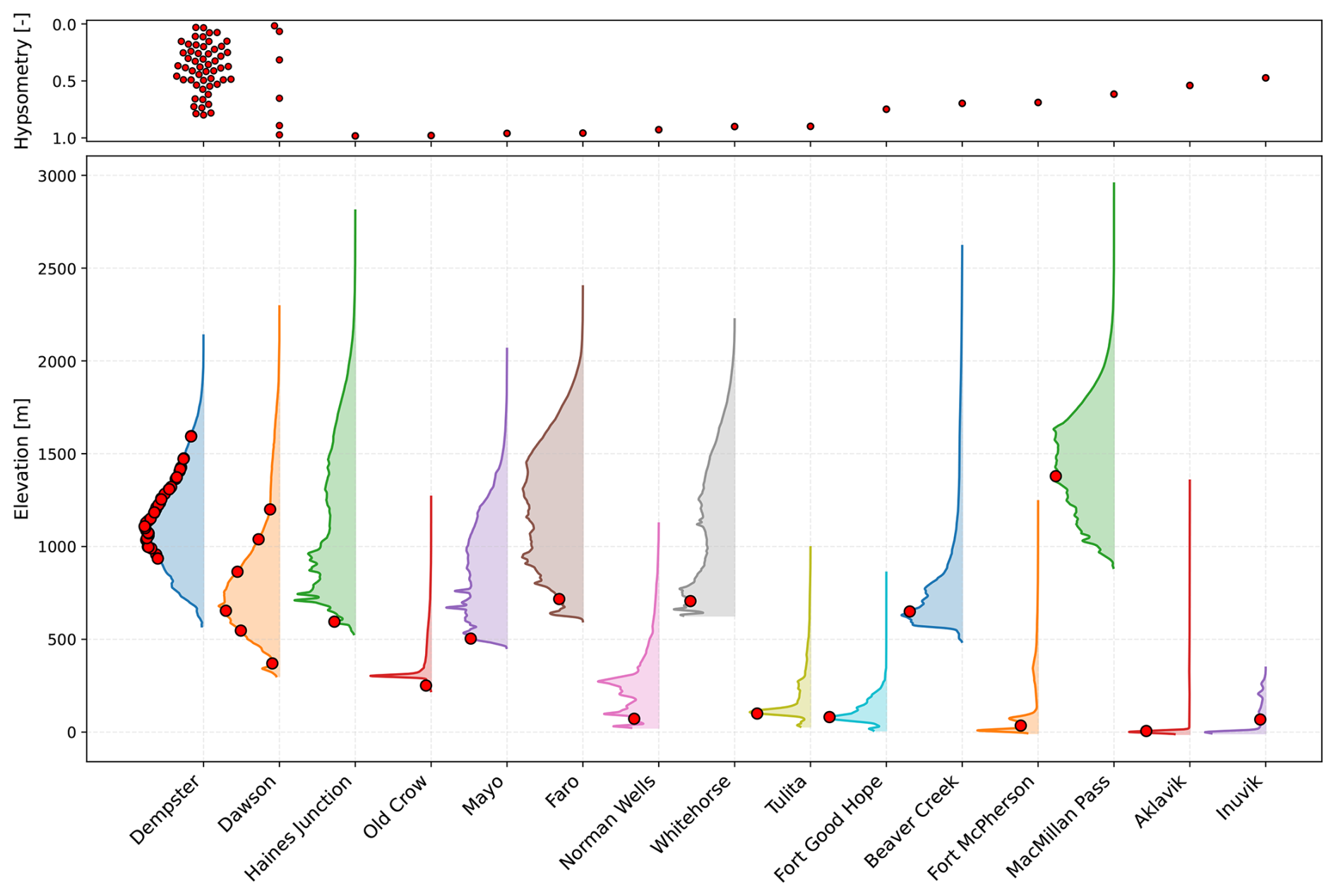
Figure 2 Local elevation distribution around each station from the study area (Dempster), the first testing area (Dawson), and the second testing area, made of 13 ECCC/NAVCAN weather stations (ranging from Haines Junction to Inuvik, sorted by decreasing hypsometry). The elevation and hypsometry of each station are indicated by a red dot.

3 Methods

3.1 In-situ observations

The 50 locations scattered across the two valleys of the study area are instrumented with passively-ventilated air temperature loggers. Air temperature data was retrieved at the end of the 2024 summer during fieldwork.

Observational data for the Dawson area is taken from Pozsgay and Gruber (2025), and was originally provided by the Yukon Geological Survey. Finally, the air temperature data for the Dawson airport and for the 10 locations described in Table E1 is managed by Environment and Climate Change Canada (ECCC) and is downloaded with the R-package weathercan (LaZerte and Albers, 2018).

3.2 Reanalysis data

Reanalysis data products are accessible globally for several decades. They are consistent and gapless in both time and space, allowing researchers to study uninstrumented areas or to provide additional data where observations might be available. In this study, we use hourly ERA5 data from the European Centre for Medium-Range Weather Forecasts (ECMWF) (Hersbach et al., 2023a, b) since 1940 and 6-hourly JRA-3Q data from the Japan Meteorological Agency (JMA) (Kosaka et al., 2024) (downscaled hourly) since 1947. The former is available on a regular 0.25°×0.25° grid in latitude and longitude, while the latter uses a TL479 Gaussian grid instead with a spatial resolution of 0.375°×0.375°. We download data divided into three categories: constant (geopotential, land-sea mask), single level (2 m temperature), and pressure levels (air temperature).

Note that at the latitude of the study area, the reanalysis grid cell approximately corresponds to a 46 km×20 km cell for ERA5, and 59 km×30 km for JRA-3Q. We downscale all reanalysis products to the stations' locations and elevations while accounting for local topography using GlobSim. Furthermore, we acquire pressure-level air temperature T_pl for a full column above each valley from the highest station upwards, at each available pressure level. For both products, we also interpolate single-level 2 m surface temperature T_sur. This is now automated with the addition of the new DReaMIT module into GlobSim.

3.3 Temperature inversion model

3.3.1 Basic structure

Pozsgay and Gruber (2025) demonstrated that downscaled reanalysis data, both single-level surface temperature T_sur and pressure-level temperature T_pl, fail to capture the full vertical profile of surface-based inversions. T_pl generally performs better at approximating the observed temperature than T_sur at higher elevation, while the use of T_sur is preferable at lower elevation, in agreement with the previous comment about the lack of reliability of pressure level reanalysis data below grid level.

To bridge the gap between the two reanalysis variables and their non-intersecting domains of reliability, a dynamic model of temperature inversions was proposed in Pozsgay and Gruber (2025). This model was calibrated for sites in the vicinity of Dawson City, Yukon, Canada, an area subject to strong temperature inversions. The model was shown to predict air temperature better than either T_pl or T_sur, for virtually any combination of elevation, time, and reanalysis product.

Thanks to the full hourly-downscaled vertical profile of air temperatures above each valley, the upper-troposphere lapse rate is computed and updated hourly. The linear relation can be extrapolated to the grid level and the station's elevation, where we define T_{lapse grid} and T_{lapse station}, respectively. The difference between the surface temperature given by reanalysis and the would-be temperature without any inversions at the grid level is given by $\text{DT}=T_{\text{sur}}-T_{\text{lapse grid}}$. The equivalent definition at the station's elevation reads ${\text{DT}}_{\text{station}}=T_{\text{obs}}-T_{\text{lapse station}}$, which corresponds to the SBI_mag metric from Noad et al. (2023). The former model simply states that the inversion's strength α is a linear function of the elevation z,

$$\begin{array}{}\text{(1)}& {\displaystyle }{\displaystyle }{\text{DT}}_{\text{station}}=\mathit{\alpha }\left(z\right)\cdot \text{DT}+\mathit{\beta }\left(t\right),\end{array}$$

where the function β is a pure temporal regional reanalysis bias, and only depends on the reanalysis product, the study area, and the seasonality, not on the elevation. Note that the temporality of the inversion strength is fully characterized by the temporality of DT, a derivative of reanalysis variables.

In Sect. 4.2, we will analyze the performance of the model given in Eq. (1) applied to the “Dempster” study sites (see Sect. 2.1). We will start with the model with the exact fitted parameters of Pozsgay and Gruber (2025), that we will label as “Dawson”, and show a lack of spatial transferability of the model. Then, we will take the same model and allow for a refitting of the parameters in the α(z) and β(t) functions, with the elevation variable either remaining the absolute elevation z or being replaced by relative elevation z_rel. This will highlight the need for spatializing, finding a more adequate topographic variable, and going beyond the linear regime, which we address by proposing a new model in Sect. 3.3.2 below where the near-surface air temperature is given by Eq. (4).

3.3.2 Hypsometry

This manuscript aims to find a parameterization for the inversion model that is more general than the one proposed in Pozsgay and Gruber (2025). There, temperature inversions are successfully modelled, but the number of weather stations are limited and local calibration cannot be spatialized. Indeed, the calibration used for Dawson City is not suitable for this study area. The main reason is that cold-air pooling is not driven by absolute elevation (even though highly correlated), but rather relative elevation compared to the surrounding topography.

A simple first step would be to explore the same model but to replace absolute with relative elevation. However, a number of questions remain. First, of all, the notion of lowest point itself is ambiguous, as it depends on the radius around the station. Then, both a valley bottom and a point in the middle of a flat tundra will receive the same null relative elevation, even though the temperature inversion dynamics differ vastly between these two cases. Furthermore, such a definition does not provide any information on higher elevations. Two points can share a similar relative elevation but be close to the bottom of a steep, narrow, and deep valley on the one hand, or be on a gentle ridge on the other hand. Once again, one does not expect these two configurations to lead to similar inversion dynamics.

Thus, a suitable and generic model of temperature inversions should rely on a variable transformation of the elevation that accounts for neighbouring topographic conditions. For the rest of this paper, we will explore the use of the hypsometric position h of a point within a given surrounding area, in the same fashion as Cao et al. (2017). This new variable will be bounded between 0–1 for the highest and lowest points in the area, respectively.

The calculation of h requires a digital elevation model (DEM). We download the Arctic DEM data (mosaics) for a radius of at least 50 km around every point in the study area (Porter et al., 2023). This dataset is available at a 2 m resolution, but we choose to work with one of 10 m as we are not interested in microtopography but relative cell elevation compared to other cells in a large radius. We study the influence of selecting smaller areas in Appendix A, where we motivate the choice of an ideal radius based on empirical optimization. Next, for a given station at position x₀ (latitude and longitude) and elevation z₀, the hypsometry is computed by looking at all cells c (coordinates c) within a radius d (we will take d=50 km), and corresponds to the fraction of points with higher elevation within that area,

$$\begin{array}{}\text{(2)}& {\displaystyle }{\displaystyle }h({\mathit{x}}_{\mathrm{0}},z_{\mathrm{0}})={\displaystyle \frac{{\sum }_c\mathit{\theta }(d-|\mathit{c}-{\mathit{x}}_{\mathrm{0}}\left|\right)\mathit{\theta }(z_c-z_{\mathrm{0}})}{{\sum }_c\mathit{\theta }(d-|\mathit{c}-{\mathit{x}}_{\mathrm{0}}\left|\right)}},\end{array}$$

where θ is the Heaviside step function. In particular, $\mathit{\theta }(d-|\mathit{c}-{\mathit{x}}_{\mathrm{0}}\left|\right)$ selects DEM cells within the predefined area, and θ(z_c−z₀) further selects the ones with elevation z_c higher than the center point elevation z₀. Note that the hypsometric value h(x₀,z₀) of a station x₀ is a coordinate transformation of its elevation z₀ and is uniquely defined for a fixed radius d. However, it does vary with the radius d if we let this parameter vary too. We study the influence of applying a 2d Gaussian weight with varying standard deviation (between 1–30 km) in Appendix A. With the definition of the hypsometric position given by Eq. (2), we have $h\in [\mathrm{0},\mathrm{1}]$, with high h values indicating low positions in the surrounding elevation distribution, where cold-air pooling is more likely, whereas low h values indicate ridge or upper-slope positions, the edge cases being

$$\begin{array}{}\text{(3)}& {\displaystyle }{\displaystyle }h=\left\{\begin{array}{l}\mathrm{0}\text{on top of the highest summit},\\ \mathrm{1}\text{at the bottom of the lowest valley}.\end{array}\right.\end{array}$$

The model proposed in this study substitutes the elevation z for the dimensionless and bounded hypsometric position h used in Cao et al. (2017). There, it was used in combination with the multiresolution valley bottom flatness (MRVBF) index v (Gallant and Dowling, 2003), but we discard it here as we will find it to be superfluous in our analysis. The hypsometric model then takes the form,

$$\begin{array}{}\text{(4)}& {\displaystyle }{\displaystyle }{T}_{\text{hyps}}(h,t)=T_{\text{lapse station}}+{\mathit{\alpha }}_{\text{exp}}\left(h\right)\cdot \text{DT}+\mathit{\beta }\left(t\right).\end{array}$$

with

$$\begin{array}{}\text{(5)}& {\displaystyle }& {\displaystyle }{\mathit{\alpha }}_{\text{exp}}\left(h\right)={\mathit{\alpha }}_{\text{intercept}}+\left(\text{exp}({\mathit{\alpha }}_{\text{slope}}\cdot h)-\mathrm{1}\right),\text{(6)}& {\displaystyle }& {\displaystyle }\mathit{\beta }\left(t\right)={\mathit{\beta }}_{\text{amplitude}}\cdot \cos \left(\mathrm{2}\mathit{\pi }\right(t-t_{*}\left)\right)+{\mathit{\beta }}_{\text{bias}},\end{array}$$

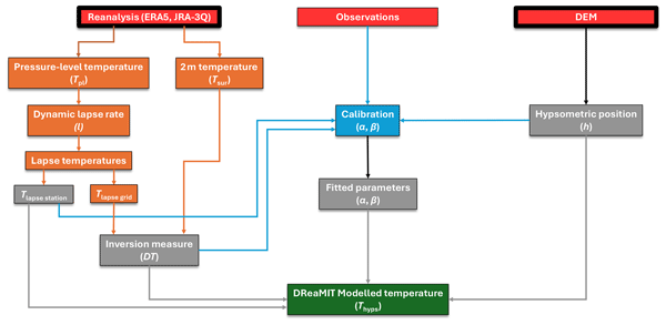
where t stands for the yearly time fraction. The wide regional reanalysis air temperature bias is independent of topography and seasonally variable, hence it is described by the sinusoidal function β(t). Note that we modify the linear α into an exponential function (which remains bounded since h itself is bounded within [0,1]). For small values of hypsometric position (h≪1), we recover the same linear α as the one of Pozsgay and Gruber (2025) to first order, since ${\mathit{\alpha }}_{\text{exp}}\left(h\right)={\mathit{\alpha }}_{\text{slope}}\cdot h+{\mathit{\alpha }}_{\text{intercept}}+\mathcal{O}\left(h^{\mathrm{2}}\right)$. The exponential correction only affects hypsometric values closer to 1, corresponding to points located in lower terrain, where inversions are likely stronger. The flowchart of the model is presented in Fig. 3. In practical application, DReaMIT requires only two inputs: (1) a digital elevation model to compute hypsometric position, and (2) reanalysis air temperatures for the neighbouring grid cells. Once calibrated, the model produces spatially-continuous hourly temperature fields across complex terrain, enabling inversion-driven corrections even at sites lacking station data, provided surrounding terrain shows meaningful valley–ridge relief.

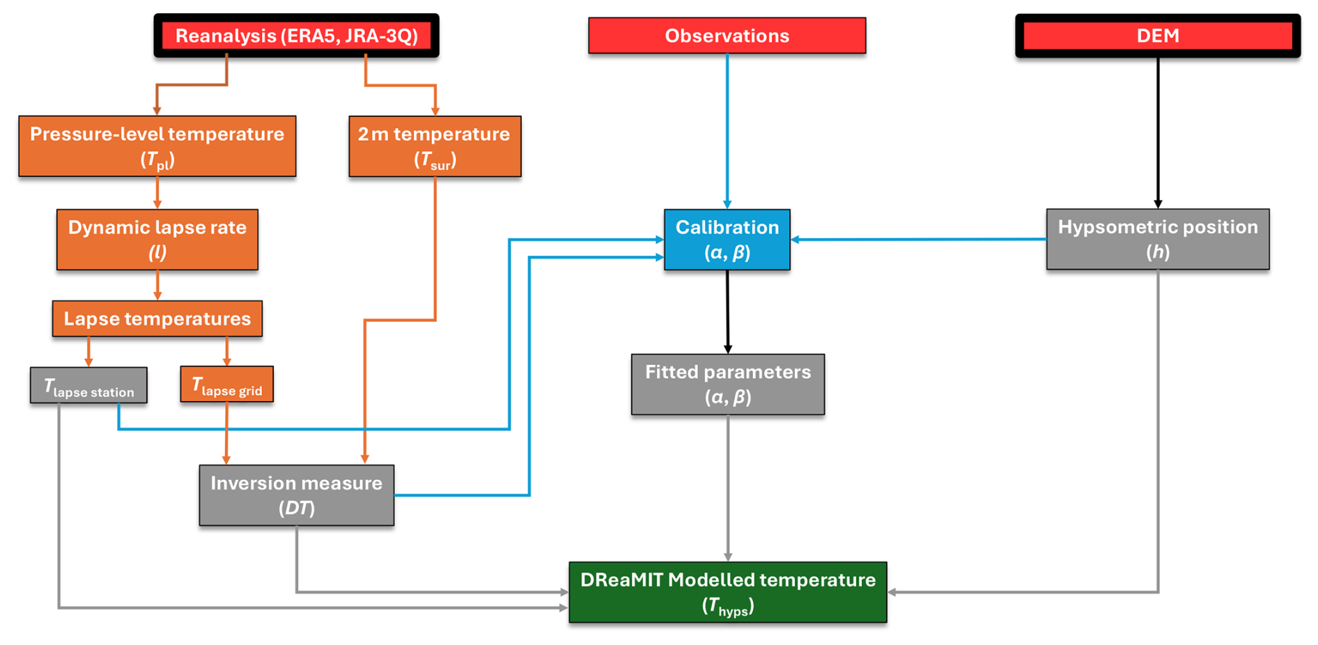
Figure 3 Flowchart of the DReaMIT hypsometric model. The input data for this study appear on the first row in red, the intermediate reanalysis steps in orange, the direct model input in grey, and the model output in green. The calibration performed in this study is shown in blue. For future cases when calibration is no longer needed, the user will only need to provide the data corresponding to cells with a thick black outline.

3.3.3 Calibration

The main advantage of a model based on hypsometric position, such as the one given in Eq. (4), is its range of applicability. Here, we no longer need to calibrate the model for each area, or even each valley; instead, we will calibrate it for both valleys of the study area at once (but independently for each reanalysis).

The data used to calibrate the model is selected to cover the widest temporal and elevational range. For each selected time, all stations with a valid record contribute to the calibration dataset. We select the maximum period for which all stations are operational, corresponding to a full year (minus 2 weeks in August, which does not bias the calibration since virtually no inversions are recorded then), and keep data at a 2 h frequency. Details can be found in Table 1. However, we will nevertheless assign a more important weight to the existing August datapoints so that each month is equally represented. Moreover, we also account for the non-uniform distribution of the hypsometric positions h in the interval [0,1] by assigning a weight to each station from Gaussian kernel density estimation (KDE). We will then perform a least-square optimization procedure to find the best model parameters for the calibration dataset. Finally, we will apply the model to the full dataset and evaluate its performance.

Table 1 Subset of the observation dataset used for model calibration. The full dataset extends over multiple years for some stations, but we choose to keep a one-year window where all stations were recording for the calibration, roughly corresponding to a third of the dataset.

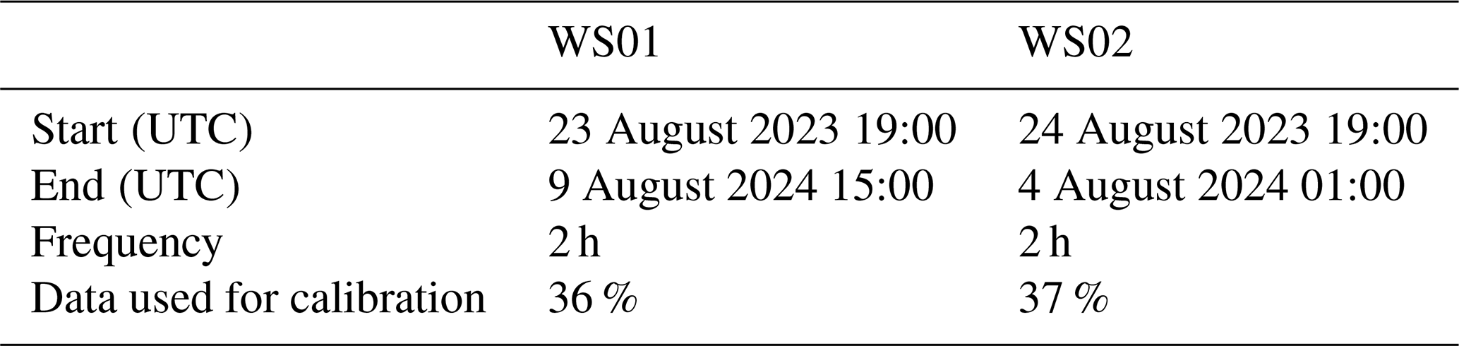
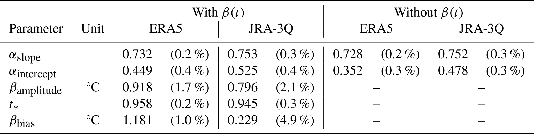
A least-square optimization is performed for all parameters of the model found in Eq. (4), on the calibration subset defined in Table 1. The calibration results can be found in Table 2.

Table 2 Best fit parameters (and their relative uncertainties in parentheses) for the calibration of the model given by Eq. (4). The model is also fitted in the absence of the reanalysis bias correction term β(t).

3.3.4 Mean alpha

To demonstrate the advantage of using hypsometric position h over (relative) elevation, we will focus on the main quantity of the model, α, i.e. the factor quantifying the strength of inversion. This factor is purely time-independent, as opposed to all other quantities in the inversion model. In order to visualize the effective α as a function of (relative) elevation, and then of hypsometry, let us start by noting that Eq. (4) can be rewritten in the following form,

$$\begin{array}{}\text{(7)}& {\displaystyle }{\displaystyle }\mathit{\alpha }={\displaystyle \frac{{\text{DT}}_{\text{station}}-\mathit{\beta }}{\text{DT}}},\end{array}$$

for every datapoint used for the model calibration. It is more meaningful to average this formula over time to get a mean effective factor. The calibration dataset is made of data that is uniformly distributed over a 1-year span (up to a small gap taken into account in the calculations but omitted here for the sake of the argument), and hence the temporal average corresponds to a yearly mean. Let us denote the yearly mean of a quantity 𝒬 with $\stackrel{\mathrm{‾}}{\mathcal{Q}}$,

$$\begin{array}{}\text{(8)}& {\displaystyle }{\displaystyle }{\mathit{\alpha }}_{\text{effective}}={\displaystyle \frac{{\stackrel{\mathrm{‾}}{\text{DT}}}_{\text{station}}-\stackrel{\mathrm{‾}}{\mathit{\beta }}}{\stackrel{\mathrm{‾}}{\text{DT}}}},\end{array}$$

and note that because of the oscillatory nature of the reanalysis bias β(t), we have $\stackrel{\mathrm{‾}}{\mathit{\beta }}={\mathit{\beta }}_{\text{bias}}$, whose value is updated and fitted separately for each case. In more details, it is possible to compute mean annual values ${\stackrel{\mathrm{‾}}{\text{DT}}}_{\text{station}}$, $\stackrel{\mathrm{‾}}{\text{DT}}$, and constant β_bias for each station individually, and from there, inferring an effective value α_effective given Eq. (8) above. When repeating this analysis over a large set of stations, we can produce a scatter plot of mean individual effective α as a function of an elevation variable, it being elevation itself, relative elevation, or hypsometry. These points are diagnostic quantities derived from observations and reanalysis, not directly observed parameters. Such results are presented in Sect. 4.2 and Fig. 4. The various fitted models of α aim at finding a global (within the acknowledged limits) functional form with respect to an elevation variable. Here, α_effective is computed independently for each station and can give an insight on the model's target.

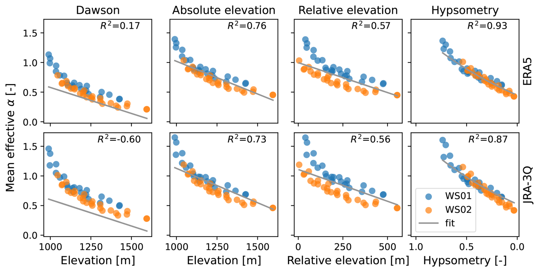
Figure 4 Mean effective and modelled values of the factor α(h) for various temperature inversion models and reanalyses.

4 Results

4.1 Fitted parameters

The relationship between hypsometric position and elevation depends on the area from which the hypsometric position is calculated, and the chosen weighting scheme. We find that the best fit is obtained when no weighting is performed (see Appendix A), which simplifies the approach.

We calibrate the model from Eq. (4) with a subset of the full dataset (see Table 1), where a least-squared fitting method is applied. The input data needed to calibrate the model are the hypsometric position on one side, which is calculated from a DEM, and reanalysis data on the other side (we use both ERA5 and JRA-3Q). The best fit parameters and their uncertainty are reported in Table 2. Note that we also fit the model in the absence of the reanalysis bias correction term β(t). This reduces the model performances but increases its versatility and applicability in certain cases presented in the Discussion (Sect. 5).

The temperature inversion model REDCAPP (Cao et al., 2017) makes explicit use of both hypsometric position h and MRVBF index v. We find that the Akaike and Bayesian information criteria (AIC and BIC, respectively) do not improve when explicitly accounting for v in the model, which motivates the functional form adopted in Eq. (4), where the temperature inversions only depend on the hypsometric position h.

4.2 Comparing different models

We present a comparative analysis on the full northcentral Yukon valleys WS01 and WS02 dataset, which aims to put the performance of the new hypsometric model in context by comparing it to various other models in Fig. 4. The first three comparisons are essentially variants of the same Pozsgay and Gruber (2025) framework, differing in calibration and the topographic variable used, whereas the hypsometric DReaMIT formulation represents the substantive model development in the last column. The first model (“Dawson”) is the inversion model proposed in Pozsgay and Gruber (2025), with their calibrated parameters. The second column, labelled “Absolute elevation”, uses the same model but with parameters specifically calibrated for the combined WS01 and WS02 valleys. The third column uses relative elevation with respect to valley bottom instead of absolute elevation, and the final column is the hypsometric model of this study. The “Dawson” model and parameters perform very poorly in this study area with a coefficient of correlation of 0.17 for ERA5 but even as low as −0.60 for JRA-3Q, confirming what was already known, i.e. it is a model that needs to be calibrated locally, which is done in the second column with much better agreement (R²=0.76 and 0.73 respectively). However, there is a clear distinction between the valleys, with values from WS01 above those of WS02. This is even more visible when looking at relative elevation, where the decoupling between the two valleys becomes so large that the model is clearly inappropriate. However, when turning to the more intricate variable transformation of elevation that hypsometry is (fourth column), we see that both valleys align, and a single model can now be applied confidently in different geographical locations. The correlation coefficient of the mean effective α over the full dataset with respect to the modelled α is equal to R²=0.93 in the case of ERA5, and 0.87 for JRA-3Q. This visually demonstrates why absolute and relative elevation do not fully spatialize the relationship, while hypsometry largely collapses the two valleys onto a common functional form.

Finally, we also perform single-valley calibration, and demonstrate the stability of the results when applied to the other valley in Appendix B. This constitutes a first step towards demonstrating the spatialization power of the model.

4.3 Application to other sites

4.3.1 Dawson area

To evaluate the performance of the hypsometric model Eq. (4) outside the study area we make use of the weather data from the stations around Dawson City, Yukon, located more than 100 km away from the two Dempster Highway valleys where the hypsometric model is calibrated. For each of the five stations, we download reanalysis data, scale it to the point locations, compute the lapse rate of their respective air columns, and download the ArcticDEM locally to transform elevation information into hypsometric position h.

The results are shown in Fig. 5 below (left panel), and in Appendix C. For each station, we present the statistical metrics MAE and R² as a function of hypsometry, for the new hypsometric model, compared to the worst of the surface and pressure-level temperatures given from reanalysis data (downscaled using GlobSim, Cao et al., 2019). We compare to the worst of T_pl and T_sur since we cannot know a priori which will be best (Pozsgay and Gruber, 2025). A more complete comparison is presented in Appendix C. Note that we average results for ERA5 and JRA-3Q and present a relative change rather than absolute metrics. Positive values indicate better predictions from the model compared to reanalysis. However, it is interesting to note that the hypsometric model (whose parameters are given in Table 2 and set once and for all) predicts air temperature more consistently than either surface or pressure-level reanalysis data. We recall the fact that the pressure-level reanalysis data performs best at higher elevation (low h, milder inversions) while the strong inversions at the valley bottom (low elevation, high h) are better represented by the surface temperature of the reanalysis data.

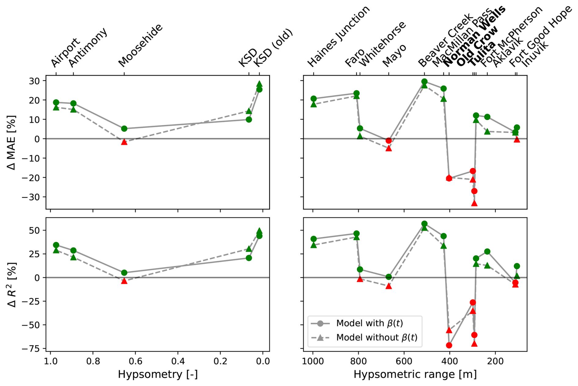
Figure 5 Statistical metrics for model vs. observations. The hypsometric model calibrated with and without the reanalysis bias term β(t) is compared to the worst of T_pl and T_sur (respectively corrected or not with β(t)) for MAE and R². Green markers indicate better predictions from the model than reanalysis, while red is worse. Stations where the hypsometric model performs worst overall appear in bold. (left) The 5 locations around Dawson City. (right) Same metrics for the 13 ECCC/NAVCAN weather stations in the Yukon and Northwest Territories. The hypsometric range is the product of (a) the hypsometric position and (b) the elevation range excluding outliers (the elevation difference between the 90th and 10th percentiles in the area around the point location).

In the situation where the user wishes to apply the model to an area where the reanalysis bias could be different than the one from Table 2 (column with β) and where no weather stations are available to calibrate β, a good alternative is to use the model calibrated without the β term (column without β of Table 2). In this case, the results are slightly worse than with the β term (except for the low h stations), but continue to outperform the reanalysis products. Once again, when no reanalysis correction is applied for the model and T_pl and T_sur, results are negatively affected but maintain the same order of magnitude. The same conclusions apply.

4.3.2 Network of northern ECCC stations

In this Section, we perform a similar analysis, but extend the testing further away, comparing the model results to the observations at 13 ECCC/NAVCAN weather stations across the Yukon and the Northwest Territories (NWT). Results are reported on the right panel of Fig. 5. The horizontal axis represents the hypsometry, modulated by the potential to drive temperature inversions. If we write dz the difference in elevation between the 90th and 10th percentiles in the area around each point location, then the hypsometric range is given by the product h⋅dz.

For stations with lower hypsometric range, i.e. milder topography, the hypsometric model (with and without reanalysis bias correction) offers better predictions than reanalsysis data. However, it has poorer performances for intermediate values of the hypsometric range, especially for Tulita, Old Crow, and Norman Wells. When the hypsometric range increases further, the best increase in reliability is observed, reaching a maximum at Beaver Creek with a 30 % and 57 % lowering of the MAE and (1−R²), respectively. Particularly good performances are also observed at MacMillan Pass, Faro, and Haines Junction.

5 Discussion

5.1 Use of hypsometry instead of (absolute) elevation

The new surface-based inversion model proposed in this study spatializes the model of Pozsgay and Gruber (2025) while making the calculation of the REDCAPP lapse rate (Cao et al., 2017) dynamic. The factor that controls the strength of the temperature inversion events, α, is modified by considering hypsometric position instead of elevation. With this choice, we successfully unify the functional form of α as a function of a variable transformation of elevation for dissimilar valleys (Fig. 4). A single calibration can now be performed simultaneously for the two valleys (WS01 and WS02) of the study area, and the resulting model is reliable in both valleys. To show that the model is indeed robust against spatialization, we perform cross-valley calibrations and find it to be reliable there too (Fig. B1).

5.2 Physical interpretation of nonlinearity

Another improvement compared to the “Dawson” model is the exponentiation of the elevation variable, instead of the linear form of α. The functional form of the proposed α_exp in Eq. (5) reduces to the linear form of Pozsgay and Gruber (2025) for locations with h≪1, while allowing for the representation of stronger inversions when h≲1, a frequently observed phenomenon.

SBIs in high-latitude valleys often exhibit non-linear lapse-rate profiles (Tikhomirov et al., 2021), where strong temperature stratification near the surface transitions to weakly stratified or isothermal layers above (Mayfield and Fochesatto, 2013). This pattern was observed in the subarctic valleys used to calibrate this model (Noad and Bonnaventure, 2026). During an SBI, lapse rates typically decayed exponentially within the first roughly 150 m where they often exceeded 25 °C km⁻¹ within the lowest 60 m and then approached isothermal above 150 m. In extreme cases, there was as much as 8 °C temperature increase over 19 m between the valley bottom and adjacent slope site (Noad and Bonnaventure, 2026).

The exponential function therefore better captures the observed behaviour of mean inversion strength (last column of Fig. 4), while being safe from unwanted divergence given the boundedness of the hypsometric position ($h\in [\mathrm{0},\mathrm{1}]$). Nonetheless, the correction is still slightly underestimating the inversion strength for the points with higher hypsometry (last column of Fig. 4). For the readers who might be surprised not to find a better fit of the mean effective α, we would like to reiterate that the fit presented there is the full model calibrated with hourly data in both valleys, and not a direct fit of mean yearly effective α.

5.3 Spatial transferability and scope of applicability

The model described by Eq. (4) was tested across a wide geographical range in Yukon and Northwest Territories, encompassing topographic diversity (Fig. 2). The hypsometric model is more versatile than any of the reanalysis temperatures, even far from the calibration study area, which proves the success of this new formulation. Model performance in Whitehorse, Haines Junction, and MacMillan Pass, which are locations that experience weaker and more transient inversions than the subarctic valleys along the Dempster Highway (Lewkowicz and Bonnaventure, 2011; Noad et al., 2023; Garibaldi et al., 2024), remained surprisingly strong. This suggests that while the model was calibrated for more continental Dempster valleys, it captures the underlying structure of SBIs well, and that its transferability extends to regions with comparable hypsometric ranges. In these settings, the model appears to represent topographic constraints on cold-air pooling processes that develop within landscapes characterized by large hypsometric range. Although the frequency and intensity of SBIs are less at Whitehorse, MacMillan Pass, and Haines Junction, their structure likely resembles those of the Dempster sites.

However, the model's transferability has limits. First of all, the inclusion of a reanalysis bias correction term β creates issues. Indeed, reanalysis bias is not uniform in time (see Fig. 7 of Fiddes and Gruber, 2014), but more importantly, it varies in space while the model explicitly assumes a spatially-independent β(t). Such a term increases model performances in a region of applicability, but is not appropriate for applications elsewhere. Instead, for such locations, we recommend either recalibrating β locally if nearby weather stations exist, or using the model calibrated without the β term (right column of Table 2), which increases the model's versatility. We showed that model performances are only minimally affected in the absence of reanalysis bias correction, demonstrating that the spatial scale at which the model can be applied is not limited by the scale over which the reanalysis bias varies. Second, the model performed poorly for certain ECCC stations, including Tulita, Old Crow, and Norman Wells. As shown in Fig. 2, these locations correspond to those with higher hypsometry, while not in a mountain area. The topography for these areas is mainly flat (the elevation distribution peaks around the elevation of the lowland), and hence, any slight elevation variation has a disproportionate effect on the hypsometry. This is a limiting case of the model. Note that for Old Crow and Tulita, the calculated value of h is close to 1, but the stations are nowhere close to being at the bottom of a deep valley. This constitutes an extreme topographic situation where the model might not be suitable. These exceptions highlight the limits of the domain: in extremely flat, river-dominated terrain, hypsometry becomes unstable and river-generated warm anomalies overwhelm the topographic signal the model relies on. In this context, the inclusion of the MRVBF in a more intricate model might mitigate this undesirable effect by better distinguishing flat from incised terrain.

A related limitation arises in generally flat areas with a low range in hypsometry. Attempts to incorporate a modified variable, a bounded version of the hypsometric range h⋅dz, which accounts for the topographic potential to sustain inversions did not substantially improve performance. Similar challenges have been reported in other lapse rate-based downscaling studies, where the absence of pronounced topographic relief often reduces the prediction of elevation-derived parameters (Fiddes et al., 2022). In such environments, microtopographic indices such as MRVBF used in REDCAPP (Cao et al., 2017) may provide complementary information on the structure of SBIs and resulting elevational patterns of air temperature. This metric, or something similar, could be used as a mechanism, to limit hypsometry closer to 0 in these flat areas.

Our results indicate a clear domain limit: stations situated on low-relief floodplains on the leeward side of mountain ranges (e.g. Norman Wells, Tulita, Old Crow) exhibit degraded performance relative to incised valleys. There, the dominant controls on near-surface temperature are not primarily terrain-controlled cold-air pooling. In these locations, river influence, floodplain energy balance, weak relief, and possible reanalysis/grid elevation artefacts may dominate over the hypsometric signal. In such settings, the gravitational pooling that sustains surface-based inversions (SBIs) is weak because slopes and basin geometry are minimal; small uncertainties in hypsometry are therefore amplified, especially when the seasonal temperature contrast DT is large. Leeward positioning further reduces inversion persistence via mechanically-driven mixing and episodic flushing (Hrebtov and Hanjalić, 2017; Dice et al., 2024), while riverine processes (late freeze-up, open water, advective heat) can imprint non-orographic thermal anomalies during transition seasons (Park et al., 2020; Prowse et al., 2007). Together, these factors yield a near-surface temperature structure that is not primarily topography-controlled, and our hypsometry-based correction can over-adjust. We therefore recommend caution for leeward floodplain sites, particularly those proximal to major rivers. In this configuration, the better-performing air temperature is T_sur. This framing clarifies that the model performs as intended in incised, terrain-controlled valleys, while transferability is limited where floodplain and river energy budgets dominate boundary-layer thermodynamics.

5.4 Scale effects on hypsometry

We focused some effort into determining the best radius around each point location to compute the hypsometric position, and concluded that even though there might exist intermediate radii for specific configurations, the most robust option was to consider a radius of 50 km, with no weighting. Recent studies have shown that the interplay between large-scale synoptic conditions and local radiative and cold-air drainage processes is scale-dependent, with larger valley systems having a more complex interaction between the two mechanisms (Crosman and Horel, 2017; Hughes et al., 2015; Sheridan, 2019). This suggests that the radius that performs best empirically (50 km) is of the order of the physical scale at which local drainage and synoptic influences control SBI strength, providing a physical rationale for the effective use scale for hypsometric position used in our model.

We showed the existence of a hierarchy of scales, with a local minimum in model performance reached for local valley scales (roughly 5 km radius for the study area), but a global and potentially location-independent best fit at larger scales (Appendix A). However, the physical scales controlling cold-air pooling and inversion persistence in the western Canadian Arctic may differ from those in other regions, and thus the relationships should be interpreted cautiously. Moreover, considering larger areas in the hypsometry calculation is yet to be tested for various topographic conditions across the western Canadian Arctic.

In subarctic environments, SBIs are sustained over periods of days to weeks rather than hours. During these events, cold-air pooling reflects not only local slope drainage (acting over scales between 1–10 km) but also the cumulative redistribution of cold air across interconnected valley systems. Consequently, the relevant topographic control extends beyond the immediate valley and may be better represented by landscape-scale hypsometric position than by local relief alone. We have used a radius arising from the data available and satisfying these approximate characteristic scales, while potentially interacting with the effective resolution of the reanalysis grid cells.

6 Conclusions

The hypsometric temperature inversion model proposed in this study is a spatialized and dynamic surface-based inversion model. Previously, it was shown that there exists a simple relationship between inversion strength and elevation for a specific area. However, this relationship varies spatially, meaning it would need recalibration for every new location. Here, we find a variable transformation of elevation (hypsometry) that preserves the shape of the inversion strength (function α) across dissimilar valleys. This new approach reuses one of the REDCAPP (Cao et al., 2017) parameters while disregarding the valleyness index (MRVBF), which was shown not to decrease the amount of information lost by the model. The DReaMIT hypsometric model combines the spatialization of REDCAPP and the dynamic lapse rate calculations of Pozsgay and Gruber (2025), while retaining a simple expression and a minimal number of dependent variables.

We then started to test the model transferability by showing the high performance of cross-valley calibration, i.e. calibrating the model in a valley and testing it in another. This first step towards a proof of the spatialization power of the model was then followed by a larger test in the Dawson City area, and across numerous ECCC stations in the Yukon and Northwest Territories. It was found to be the most robust and reliable model of air temperature when compared to raw reanalysis data and the “Dawson” model. This does not mean that the hypsometric model always performs best, but rather that it is, on average, the preferred option. However, we issue recommendations for the best use of this model: (a) use when the hypsometry is well-defined, i.e. when small variations in elevation do not lead to dramatic variations in h, (b) for applications outside of the western Canadian Arctic, recalibrate the reanalysis bias β locally with weather station data when available, or use the “no-β” version of the model otherwise. In other words, DReaMIT is most appropriate where hypsometry is well-defined by meaningful surrounding relief, and users should be cautious in low-relief floodplain settings or where local non-orographic controls dominate the near-surface thermal regime. With this caveat in mind, we thus present a reliable, spatialized, and dynamic model of temperature inversions for the mountainous western Canadian Arctic.

Appendix A: Relative importance of the radius of the hypsometric position

The hypsometric position was defined in Eq. (2). We here study the influence of adding a 2d Gaussian weight modulating the typical spatial scale of the inversions. Here, we weigh each cell c with a Gaussian weight with standard deviation r,

$$\begin{array}{}\text{(A1)}& {\displaystyle }{\displaystyle }{h}_r\left({\mathit{x}}_{\mathrm{0}}\right)={\displaystyle \frac{{\sum }_c\mathit{\omega }(r,|\mathit{c}-{\mathit{x}}_{\mathrm{0}}\left|\right)\mathit{\theta }(d-|\mathit{c}-{\mathit{x}}_{\mathrm{0}}\left|\right)\mathit{\theta }(z_c-z_{\mathrm{0}})}{{\sum }_c\mathit{\theta }(d-|\mathit{c}-{\mathit{x}}_{\mathrm{0}}\left|\right)\mathit{\omega }(r,|\mathit{c}-{\mathit{x}}_{\mathrm{0}}\left|\right)}},\end{array}$$

where the weights are defined by

$$\begin{array}{}\text{(A2)}& {\displaystyle }{\displaystyle }\mathit{\omega }(r,|\mathit{c}-{\mathit{x}}_{\mathrm{0}}\left|\right)=\exp \left\{-{\displaystyle \frac{|\mathit{c}-{\mathit{x}}_{\mathrm{0}}{|}^{\mathrm{2}}}{\mathrm{2}{r}^{\mathrm{2}}}}\right\}.\end{array}$$

We can also compute the multiresolution valley bottom flatness (MRVBF) index (Gallant and Dowling, 2003), which is an index that parameterizes the valleyness of a given point.

The hypsometric position, as defined by Eq. (2) (or in Eq. A1 for its weighed version), is a variable transformation of the absolute elevation. It carries information not only on the elevation of the point of interest, but also on the neighbouring terrain, or neighbouring cells if the terrain is discretized, such as in a DEM. The choice of the radius within which elevation information is retained reflects the scale at which the processes happen. For small radii, the local topography bears more importance, whereas it is increasingly smoothed with increasing exponential weight radius.

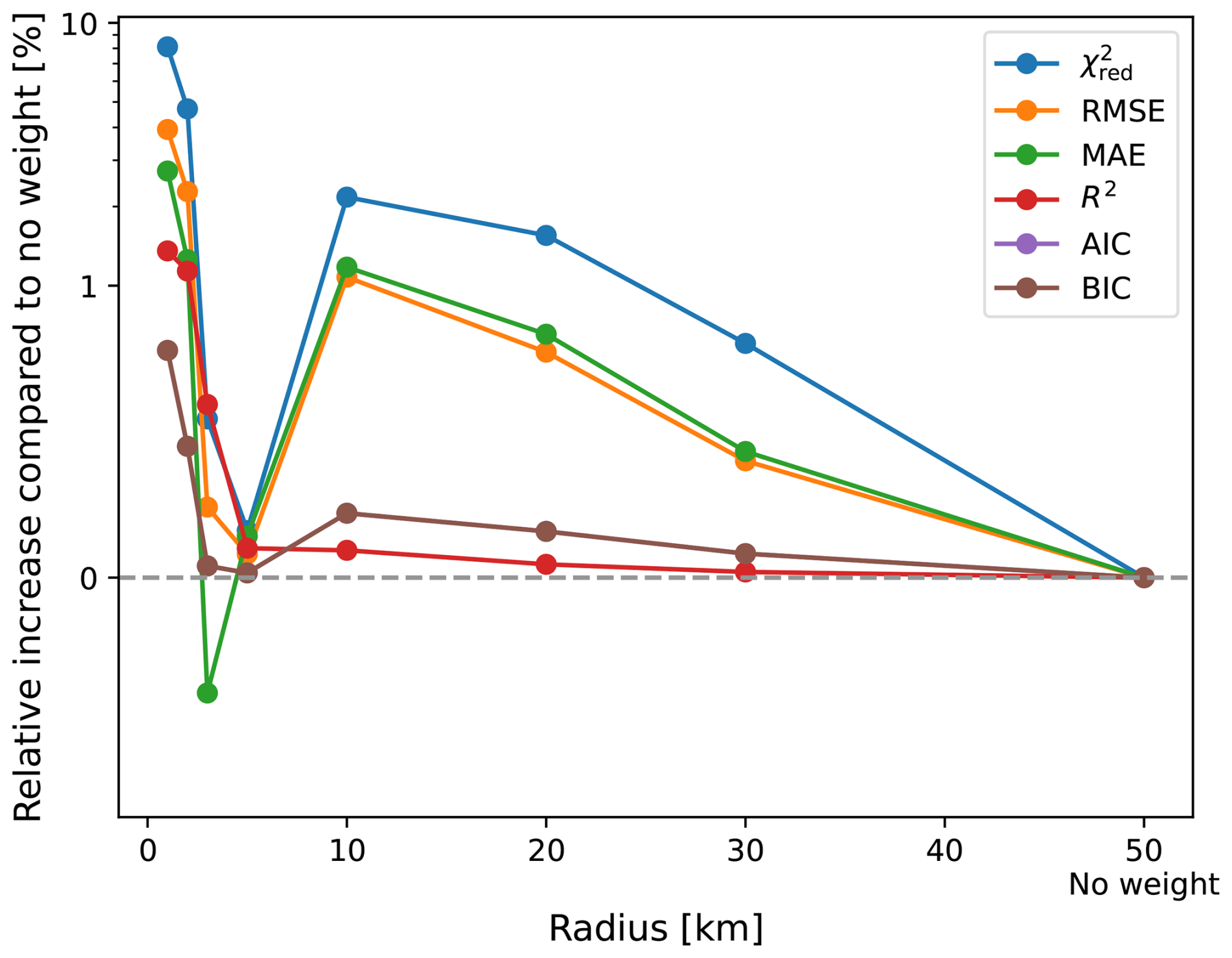
Figure A1 Comparison of the goodness of fit for the model calibration at different radii r, with respect to the limiting case without Gaussian weight.

For each Gaussian weight radius r, we perform the calibration and evaluate the goodness of fit by computing different statistical metrics: root mean square error (RMSE), mean absolute error (MAE), reduced chi-square (${\mathit{\chi }}_{\text{red}}^{\mathrm{2}}$), coefficient of correlation R², and both Akaike and Bayesian information criteria (AIC and BIC respectively). They are compared to equivalent results for the case where no weight is applied, which is the optimal case (see Fig. A1). The results improve quickly with increasing radius r, up to r∼5 km, where the goodness of fit finds a local minimum. Further increasing the Gaussian weight radius leads to worse agreements with observations for the model calibration, until r∼10 km. After this maximum, all metrics improve again, and the limiting case where no weight is applied is found to lead to the best agreement between model and observations for the calibration dataset.

We established the influence of the standard deviation of the 2d Gaussian weight r, not only in the value of h itself, but also in the performance of the inversion model. For each radius, reanalysis, and stations, the mean effective α_exp is computed and plotted in Fig. A2. The exponential line of best fit is obtained from the calibrated parameters of the model (see Table 2 for the parameters used in the last column labelled “No weight”). The line of best fit is thus not obtained directly at the level of the mean α_exp. However, the values of the correlation coefficient R² in Fig. A2 correspond to the correlation between mean effective α_exp and modelled α_exp, i.e. for a dataset consisting of a single point per station. The value of R² starts as low as 0.30 and 0.29 for a radius of 1 km for ERA5 and JRA-3Q, respectively, and steadily increase until r=10 km where they reach R²=0.91 and 0.84, respectively. Further increasing the radius, or even dropping the 2d Gaussian weights altogether, has little to no impact on the correlation coefficient. However, the best agreement here too is found when no weighting scheme is applied (where 92 % of the variability in the mean effective α_exp is explained by the model for ERA5, and 86 % for JRA-3Q). This further motivates our choice to focus our analysis on this case.

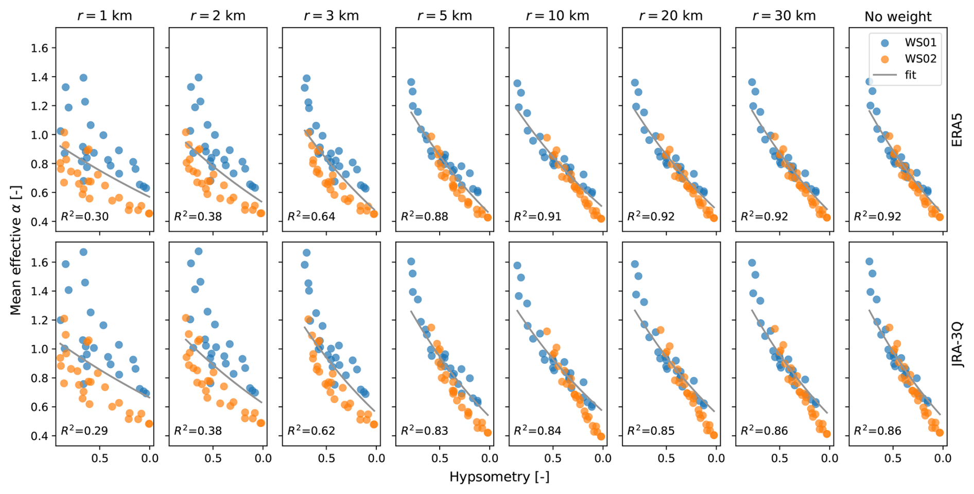
Figure A2 Mean effective values and calibration fit of the factor α_exp(h) for different radii and both reanalysis products.

Appendix B: Swapping valleys

We perform single-valley calibrations, and apply the resulting fitted parameters to the other valley for all data points and not just the calibration dataset. This allows us to show the applicability of the model outside of its calibration area. In Fig. B1, we plot the same quantities as in the Sect. 4.2, i.e. mean effective α against hypsometry, overlaid by a line representing the modelled α, whose parameters are either calibrated for both valleys at once (first column), or for each valley independently (next two columns). The values of the coefficient of correlation are given for all stations in black, and for stations of individual valleys WS01 and WS02 in blue and orange, respectively.

When the model is only calibrated using a year of data from WS01 (second column), the calculated values of α (for all data points and not solely the calibration set) explain 85 % and 78 % (for ERA5 and JRA-3Q) of the variation of the mean effective α in the valley WS01, however this drops to respectively 79 % and 60 % when applying it to WS02. Now, the calibration of WS02 for WS01 performs much better, with correlation coefficients as high as 0.84 for ERA5 and 0.80 for JRA-3Q. Note that the cross-valley modelling is better when calibrating on WS02 because its own calibration results are better than WS01. Indeed, the shape of the mean effective α as a function of the hypsometric position h is more closely aligned with the exponential choice of fitting function for WS02 than WS01, and hence the poorer performance of the WS01-calibrated WS02 model is directly inherited from the relatively poorer performance of the WS01-calibrated WS01 model. The WS02-calibrated WS01 model (third column) is largely successful, which demonstrates the wider scope of this model, beyond its own calibration area.

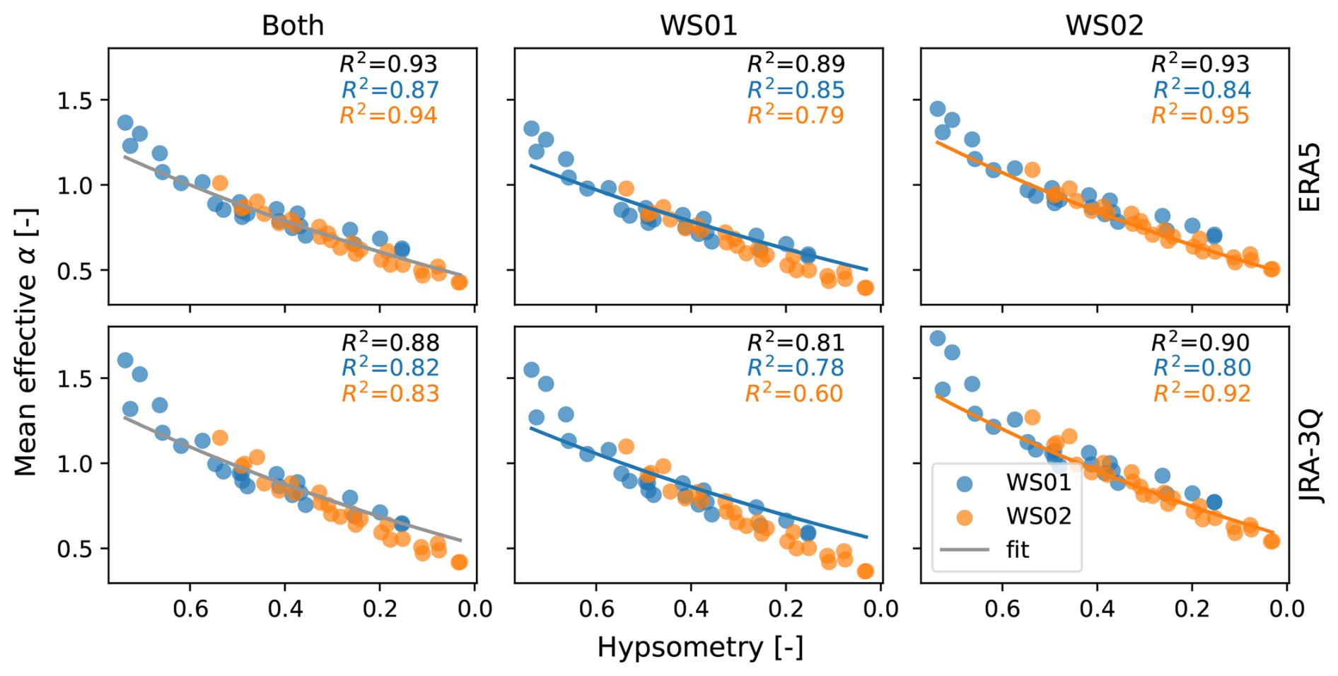
Figure B1 Mean effective and modelled values of the factor α(h) for a calibration over both valleys, or each valley individually, and for both reanalysis products.

Appendix C: Testing model performance relative to reanalysis products

We demonstrated that the model from Eq. (4), with and without the β term, globally outperformed the worst of the reanalyis products (corrected or not for the reanalysis bias) for the Dawson sites, and for most ECCC sites, except at intermediate to low hypsometric range. Here, we present the full picture and plot the values of MAE and R² with and without reanalysis bias correction in Fig. C1, for the hypsometric model of Eq. (4), the reanalysis products (both T_pl and T_sur), and the Dawson model of Pozsgay and Gruber (2025). For the Dawson area (left), the “Dawson” model performs the best, but this comes as no surprise, as it was specifically calibrated for the area, but was not designed to include any spatial generalizability. Whether reanalysis bias is corrected or not, the hypsometric model performs better than pressure-level temperature and worse than surface temperature for high h, while the opposite is true for low h.

For the ECCC stations (right panel of Fig. C1), stations with lower hypsometric range, i.e. milder topography, the temperature inversions are not as strong and the surface level reanalysis data is the one that performs the best, as expected. There, the hypsometric model exhibits similar values, and not worse than the pressure-level reanalysis data. For intermediate values of the hypsometric range, especially for Tulita, Old Crow, and Norman Wells, the hypsometric model seems to have poorer performance. However, it is then outperforming any raw reanalysis data at even higher values, especially for Beaver Creek.

We note that general conclusions are valid whether we look at the full hypsometric model, or the simplified one calibrated without the β term.

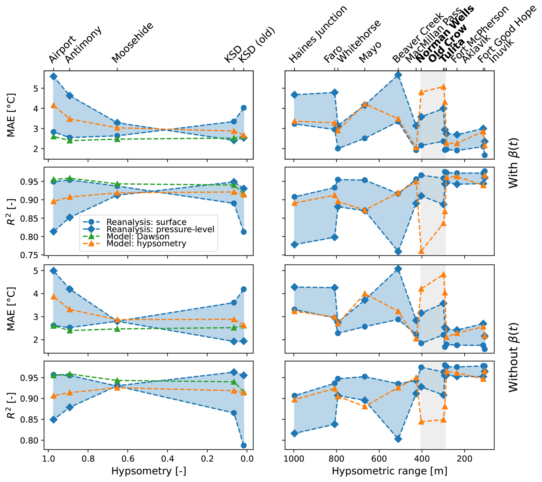
Figure C1 Statistical metrics for model vs. observations. The hypsometric model calibrated with and without the reanalysis bias term β(t) is compared to both T_pl and T_sur (respectively corrected or not with β(t)) for MAE and R². Stations where the hypsometric model performs worst overall appear in bold. (left) Comparison for the 5 locations around Dawson City, together with the model of Pozsgay and Gruber (2025) in orange. (right) Same metrics for the 13 ECCC/NAVCAN weather stations in the Yukon and Northwest Territories.

Appendix D: Study area temperature inversions

We compare the modelled air temperature given by Eq. (4) to the bias-corrected T_sur and T_pl (i.e. to which we subtracted β), for two stations from the WS01 valley. Those were chosen to represent low and high hypsometric positions. For the top row of Fig. D1, corresponding to high h, the best performing time series is the hypsometric model. The surface temperature is too low ($\text{MBE}=-\mathrm{1.60}$ °C), while the pressure-level temperature is too high, especially towards the lowest temperatures, resulting in poor MAE and R². Next, when turning to low h (bottom row), the hypsometric model is still the preferred option, but the pressure-level temperature has similar performances, except for a cold bias ($\text{MBE}=-\mathrm{0.95}$ °C). In this case, it is now the surface temperature that deviates at low temperatures, but presents a significant cold bias there. This comparison confirms the non-intersecting domains of applicability of T_sur and T_pl found in Pozsgay and Gruber (2025), while demonstrating the advantage of the hypsometric model.

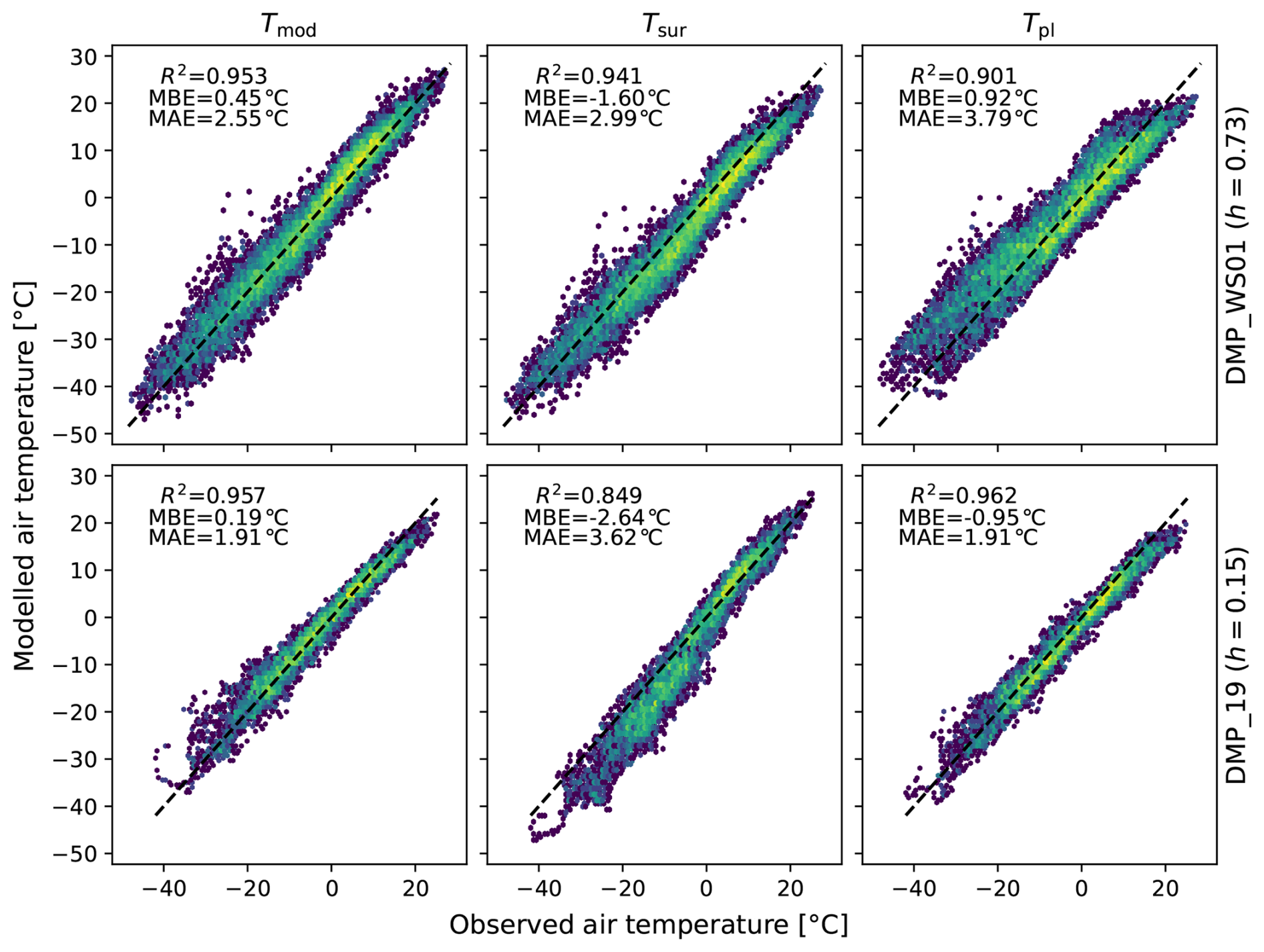
Figure D1 Parity plot of modelled vs. observed temperatures for the two stations of diverse hypsometry from WS01 valley (h=0.73 for the top row, and h=0.15 for the bottom). We compare the results of the model to the bias-corrected T_sur and T_pl.

Appendix E: ECCC stations

Table E1 Network of ECCC/NAVCAN weather stations used for air temperature data over 10 years, between 1 August 2015–31 July 2025.