Untangling the effects of vertical mixing schemes and convective adjustment in the Mediterranean Sea: insights from a sensitivity study

The Mediterranean Sea provides a natural laboratory for investigating ocean circulation processes of global relevance due to its complex dynamics, active deep and intermediate water formation, and sensitivity to climate variability. Regional ocean circulation models' skill strongly depends on the parameterization of subgrid-scale processes, among which turbulent vertical mixing and convection play a major role. To evaluate their impact in the Mediterranean Sea two-year-long simulations were conducted using three vertical closure schemes: the Richardson-number dependent parameterisation, the Turbulent Kinetic Energy (TKE) scheme, and the Generalised Length Scale (GLS) scheme. Each scheme was tested both with and without the convective adjustment approach, resulting in a set of comparative experiments designed to isolate the contribution of the adjustment process and its combined effect with each parameterization. Model results are evaluated against all available Argo floats data, both at the basin scale and in key deep and intermediate water formation regions. The simulations show that adding a convective adjustment is crucial to accurately reproduce observations with the Richardson-number dependent parameterization, where it improves all key variables, while for the TKE scheme it is particularly important for representing the mixed layer depth across the basin and in deep water formation areas. For more physics-based vertical schemes, like the GLS closure, the convective adjustment is mostly redundant and can occasionally degrade results. Overall, the GLS scheme without any convective adjustment provides the most accurate representation of the mixed layer depth as well as the vertical structure and variability both at basin scale and in key regions of deep and intermediate water formation.

1 Introduction

The Mediterranean Sea is a semi-enclosed basin characterized by intense thermohaline variability, strong mesoscale activity, and complex interactions with the atmosphere and surrounding land masses. Its dynamical features, including dense water formation, flux exchanges through narrow straits, and sub-basin circulations, make it a particularly challenging environment for ocean modeling (e.g., Pinardi and Masetti, 2000; Millot and Taupier-Letage, 2005; Testor et al., 2018). The Mediterranean Sea plays a crucial role in shaping the regional climate (e.g. Pinardi and Navarra, 1993; Lionello et al., 2006; Pinardi and Masetti, 2000) and represents a natural laboratory for investigating key ocean processes with implications at the global scale. In this sense, it is often considered a “miniature ocean” (e.g., Bethoux et al., 1999), where processes such as deep and intermediate water formation, strait exchanges, mesoscale variability, and air–sea interactions can be studied in a confined environment as a small-scale analogue of global processes.

Over the past two decades, regional ocean models have been widely employed to simulate the Mediterranean circulation at increasing spatial and temporal resolution. Among these, the physical component of the Mediterranean Forecasting System, developed within the framework of the Copernicus Marine Service, represents a state-of-the-art implementation (e.g., Oddo et al., 2009; Tonani et al., 2009; Clementi et al., 2017; Coppini et al., 2023). It provides regular, open-access analyses, forecasts (Clementi et al., 2023) and reanalyses (Escudier et al., 2021) of the basin's physical state and serves as a reference framework for scientific and operational applications.

Due to high computational costs and missing physics, the spatial and temporal resolution of current hydrostatic ocean circulation models, even at regional scale, is unable to explicitly resolve the inherently non-hydrostatic and small-scale turbulent vertical mixing and convective processes. To this end, vertical mixing closure schemes – either based on simplified formulations (e.g., Pacanowski and Philander, 1981) or on more physically based models (e.g., Gaspar et al., 1990; Umlauf and Burchard, 2003) – are employed to mimic these turbulent processes. Also, deep convection, which corresponds to the formation of dense deep water masses, has to be represented through parameterizations to reproduce its timing, intensity, and spatial extent realistically (e.g., Marshall and Schott, 1999; Villarreal et al., 2005; Herrmann et al., 2008; Luneva et al., 2019). Note that convection causes turbulent vertical mixing under unstably stratified conditions and can be parameterized separately (convective adjustment) or within the same turbulence closure scheme (Umlauf and Burchard, 2003; Legay et al., 2025).

Physics-based turbulent closure schemes include buoyancy production terms and are, in principle, able to represent convective mixing when the stratification becomes unstable. However, in practice these schemes may not always remove static instability rapidly enough, particularly at the temporal and vertical resolution typically used in regional ocean models. This can lead to an underestimation of convective mixing. For this reason, ocean circulation models usually combine turbulence closure schemes with a convective adjustment parameterization (e.g. Clementi et al., 2017; Coppini et al., 2023). The convective adjustment acts by stabilizing the water column through a rapid vertical redistribution of tracers, ensuring a prompt restoration of stable stratification. In this sense, it does not represent an independent physical process, but rather a numerical parameterization designed to mimic the fast overturning associated with unresolved convective events.

This combined approach has been widely adopted in the modelling of the Mediterranean Sea for several decades (Pinardi et al., 2003; Pinardi and Coppini, 2010), mostly because the relatively simple turbulence closure schemes traditionally employed were not sufficient to adequately represent convective mixing. In this context, it is essential to assess how these earlier, less complete schemes compare with more advanced formulations which are specifically designed to provide a more consistent and physically based representation of turbulent and convective processes. Depending on the turbulence closure scheme adopted, the use of an explicit convective parameterization may or may not be required. Assessing this aspect is one of the main objectives of the present study.

The choice of mixing scheme and convective adjustment parameterisations has been shown to play a crucial role in shaping the circulation, the temperature and salinity distributions and deep-water formation (DWF) processes (e.g., Herrmann et al., 2008; Reffray et al., 2015; Luneva et al., 2019; Robertson and Dong, 2019; Gutjahr et al., 2021). In particular, vertical mixing controls the redistribution of heat and salt throughout the water column, thereby influencing stratification and mixed layer depth (MLD). Convection, on the other hand, strongly affects deep and intermediate water formation, which in turn impacts large-scale circulation patterns and water mass properties. Since these processes are tightly coupled to air–sea exchanges and mesoscale dynamics, model sensitivity to the choice of mixing and convection schemes can propagate across a wide range of spatiotemporal scales, ultimately influencing the realism of simulated ocean variability.

Only a few previous studies provide a context for understanding the performance of different mixing schemes, but none of these explicitly investigate their combined effect with a convective adjustment, and whether a mixing scheme alone is sufficient to reproduce the vertical structure and variability of the upper ocean. Madec et al. (1991) combined Richarson-number dependent closures with nonpenetrative convective adjustment in studies of deep-water formation in the Northwestern Mediterranean Sea. Reffray et al. (2015) investigated the sensitivity of turbulent vertical mixing using a 1D ocean circulation model at the global scale, comparing various mixing schemes but without including convective adjustment. Gutjahr et al. (2021) compared various global-scale mixing schemes – including among the others, Richardson-number dependent closures and Turbulent Kinetic Energy (TKE) – but did not assess the role of convective adjustment. Storto et al. (2023) focused on the Mediterranean Sea, comparing the Generalized Length Scale (GLS) and TKE schemes, but did not examine cases of active convection and therefore did not evaluate the potential impact of including a convective adjustment. By explicitly investigating the interplay between vertical mixing schemes and convective adjustment, the present study addresses a gap left by these prior works and demonstrates how convective adjustment modulates the behaviour of different schemes in the context of the Mediterranean Sea.

The aim of this study is to investigate the sensitivity of a modified configuration of the Mediterranean Forecasting System (Clementi et al., 2023) to the choice of vertical mixing scheme and to the inclusion of an explicit convection adjustment parameterization. Model performance is evaluated across spatial and temporal scales through an intercomparison of temperature, salinity and mixed layer depth, from basin scale over years to deep and intermediate water formation regions ranging from months to hours. Given that the formation of deep and intermediate waters in the Mediterranean occurs on seasonal timescales, with interannual variability, a two-year model integration is sufficient to capture the main differences between experiments.

The rest of the paper is structured as follows. Section 2 describes the region and the observational dataset used to assess our model performances (Sect. 2.1). It also describes the model configuration (Sect. 2.2), with a focus on the choice of the vertical mixing schemes and convective adjustment, and the experimental design performed in this study (Sect. 2.3). Section 3 presents the main results of this study. We first present the impact of the convective adjustment (Sect. 3.1). Then we show results at the basin scale over the entire two-year period (Sect. 3.2). We focus then on deep and intermediate water formation regions over months to days (Sect. 3.3), and we investigate summer daily convection events at hourly temporal scales (Sect. 3.4). Finally, Sect. 4 discusses the key conclusions and outlines perspectives for future work.

2 Data and methods

2.1 Argo float data in the Mediterranean Sea

We use Argo float data (Wong et al., 2020; Poulain et al., 2007) from the Copernicus Marine Service Global Ocean near real-time in situ quality controlled observational product (whose Copernicus product name is Global Ocean-In-Situ Near-Real-Time Observations, https://doi.org/10.48670/moi-00036, E.U. Copernicus Marine Service Information (CMEMS), Marine Data Store (MDS), 2026b) as a reference observational dataset for our model validation. The location of Argo floats in the Mediterranean Sea during the two-year period under investigation (2020–2021) is reported as red dots in Fig. 1a. This dataset consists of 11 053 Argo profiles across the Mediterranean Sea, which allows for a statistically robust analysis of the processes under investigation while ensuring homogeneous quality control. Except for a few regions – such as the North Adriatic Sea, the Aegean Sea, the Strait of Sicily and the Gulf of Sirte – the Argo data in this time period provide good spatial coverage across the major part of the basin, offering a statistically meaningful dataset for our model validation.

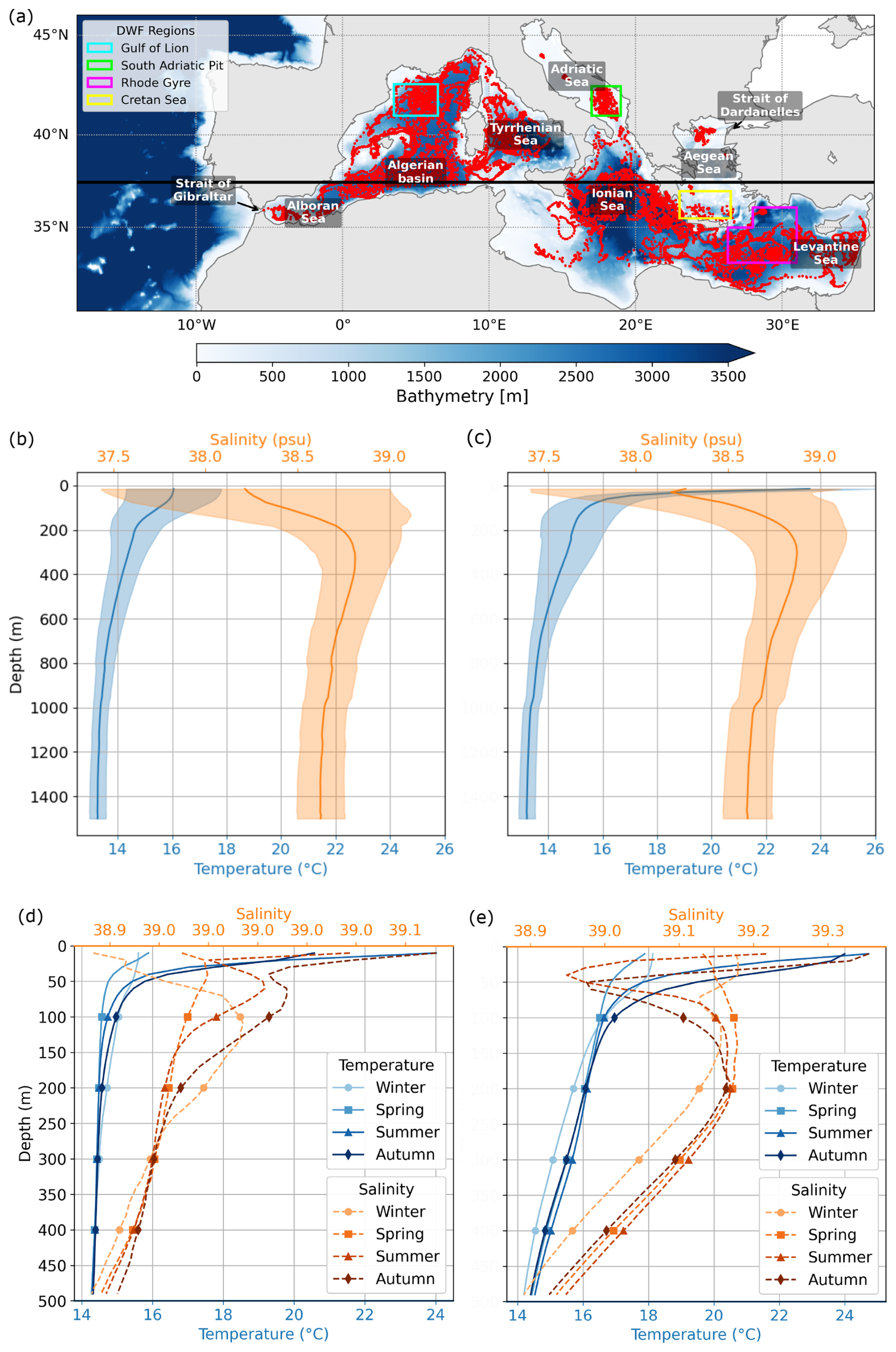
Figure 1 (a) Model domain including the Mediterranean Sea and an Atlantic box, with bathymetry as a background colour and labels for the main subbasins and deep and intermediate water formation regions. Red dots indicate Argo floats during 2020–2021. The black zonal line at 37.5° N marks the location of a vertical section used throughout the paper. Middle panels show the basin-averaged observed temperature (blue) and salinity (orange) for (b) January 2021 and (c) July 2021, where shaded areas represent one standard deviation. Bottom panels show the season-averaged observed temperature (blue) and salinity (orange) in (d) the South Adriatic Pit and (e) the Rhodes Gyre region.

Typical temperature and salinity profiles retrieved by Argo floats in the Mediterranean Sea are shown in Fig. 1 as monthly average vertical profiles of temperature and salinity in January 2021 (Fig. 1b) and July 2021 (Fig. 1c). The observations exhibit strong variability around the mean both in temperature and salinity, especially in the upper ∼200 m, highlighted by shading representing one standard deviation of the dataset. It is known that, both temperature and salinity show also a pronounced seasonal variability (e.g., Pinardi and Masetti, 2000). In winter (Fig. 1b) stratification is weakened because of surface cooling and increased vertical mixing, resulting in the formation of a thick mixed layer with relatively uniform temperature and salinity. In summer (Fig. 1c), temperature and salinity values close to the surface become higher with respect to winter as the result of strong heating and evaporation. These processes inhibit vertical mixing and give rise to a well-defined thermohaline stratification. As a result, vertical profiles are more homogeneous in winter and strongly stratified in summer.

The Mediterranean Sea hosts several key regions of deep and intermediate water formation, including the Gulf of Lion, the South Adriatic Sea, the Rhodes Gyre, and the Aegean Sea (see map in Fig. 1a). In these areas, vertical mixing and convection play a central role in preconditioning and driving dense water formation processes by modulating stratification and contributing to surface buoyancy loss. Figure 1 also shows the seasonal variability of temperature and salinity profiles from Argo floats for two of these regions: the South Adriatic Pit (Fig. 1d) and the Rhodes Gyre region (Fig. 1e). In both regions, temperature profiles exhibit a pronounced seasonal variability in the upper layers, especially near the surface, closely following the seasonality of the surface heat fluxes. On the other hand, salinity shows distinct seasonal changes associated with deep and intermediate water formation processes. In the South Adriatic Pit (Fig. 1d), the winter period (i.e., December–January–February) is influenced by the intrusion of intermediate water formed in the Levantine basin, visible as a marked salinity increase between about 100 and 200 m. Deep-water formation is not clearly visible, being largely smoothed by seasonal averaging, reflecting its short duration (order of weeks) and spatially localized nature. In the Rhodes Gyre region (Fig. 1e), where intermediate water forms, salinity shows a persistent increase throughout the year. The salinity maximum is located at about 150 m in winter, during the formation phase, and deepens to about 200 m in spring (i.e., March-April-May) and to about 250 m in summer (i.e., June–July–August) and autumn (i.e. September–October–November).

2.2 Model setup

Our model setup builds on the Mediterranean Forecasting System model of the Copernicus Marine Service. The model domain encompasses the entire Mediterranean Sea and extends into a portion of the Atlantic Ocean (Fig. 1a), spanning from 18°7.50^′ W to 36°17.50^′ E in longitude and 30°11.25^′ and 45°58.75^′ N in latitude. Including an Atlantic box is essential to accurately resolve water exchanges between the Mediterranean Sea and the Atlantic Ocean through the Strait of Gibraltar, as the inflow of fresher Atlantic water and the outflow of saltier Mediterranean water strongly influence basin-wide salinity, temperature, and density structure, as well as DWF. Nevertheless, the analysis performed in this study focuses only on the Mediterranean Sea.

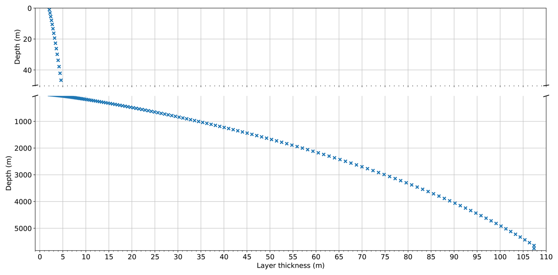
Figure 2 Vertical layer thickness as a function of depth. A zoom of the upper 50 m highlights the fine vertical discretization within the mixed layer.

The model system consists of a two-way coupled hydrodynamic circulation model and a third-generation spectral wind wave model. The ocean hydrodynamic circulation model is based on Nucleus for European Modelling of the Ocean (NEMO; Madec et al., 2022; Madec and the NEMO System Team, 2023, https://doi.org/10.5281/zenodo.6334656) version 4.2 and the wind wave model on WaveWatch III (WW3; Tolman, 2021) version 6.07. The coupling happens hourly online with the exchange of air–sea temperature difference and surface currents from NEMO to WW3, and of neutral drag coefficient used to evaluate the surface wind stress from WW3 to NEMO (Clementi et al., 2017).

The model has a horizontal resolution of 1/24° (about 4 km) in both latitude and longitude, and it includes 141 non-uniformly distributed vertical levels. The vertical layer thickness varies with depth (Fig. 2), with particularly fine resolution in the upper ocean (from about 2.1 m near the surface to 4.6 m at 50 m depth). This dense discretization in the mixed layer allows for an accurate representation of key upper-ocean processes, such as mixing and stratification, which are essential for capturing surface-driven dynamics. The time stepping is achieved within a leapfrog differencing structure associated with an Asselin filter and the baroclinic time step is set to 180 s. To capture the effects of intensified vertical mixing induced by internal wave breaking in the Strait of Gibraltar, particularly near Camarinal Sill (Wesson and Gregg, 1994; Hilt et al., 2020), we also prescribe an enhanced vertical diffusivity farther to the east of the sill.

Horizontal tracer advection is computed using the fourth-order Flux-Corrected Transport (FCT) scheme, which provides a good balance between accuracy and numerical stability by combining a high-order transport method with a monotonicity constraint (Lévy et al., 2001). Lateral diffusion of tracers is implemented as a Laplacian operator along isoneutral surfaces, with a spatially constant diffusivity. Horizontal momentum advection is treated in flux form using the third-order Upstream-Biased Scheme (UBS). As for tracers, momentum lateral diffusion is applied using a Laplacian operator along isoneutral surfaces, again with constant viscosity. These parameterisations are widely used in NEMO-based configurations for large-scale and regional ocean modelling, providing physically consistent dissipation while preserving the large-scale circulation features (e.g., Madec and the NEMO System Team, 2023; Le Sommer et al., 2009).

2.2.1 Vertical mixing scheme

In this study, we compare three different parameterisations for vertical mixing, representative of the main families of vertical mixing parameterizations commonly used in ocean modelling. Our aim is to compare more simple approaches – such as the Richardson-number dependent scheme, which is still used in the Mediterranean Forecasting system of the Copernicus Marine Service (Clementi et al., 2017; Coppini et al., 2023) – with more physically based formulations. These physics-based parameterizations rely on a prognostic treatment of turbulence and are designed to capture a wider range of oceanic mixing processes with greater physical accuracy. Physically based vertical mixing schemes typically fall into two categories: one-equation and two-equation turbulence closure models. One-equation schemes solve a prognostic equation for the TKE while relying on diagnostic expressions or empirical assumptions for the mixing length or the dissipation rate (e.g., Gaspar et al., 1990). Two-equation models introduce an additional prognostic variable – usually the turbulence length scale or the dissipation rate of turbulent kinetic energy – which allows for a more flexible and accurate representation of turbulence in stratified and sheared flows (e.g., Mellor and Yamada, 1982; Umlauf and Burchard, 2003). Each of these formulations requires calibrating several parameters. In this study, the best configuration for each scheme was selected from sensitivity tests as the one minimising statistical errors at the basin scale when compared with all available Argo data.

The first vertical mixing scheme used in this study is a Richardson number-dependent formulation originally proposed by Pacanowski and Philander (1981). This scheme was originally developed for the equatorial ocean, using a rectangular box model, and was not designed to provide prognostic mixing. Vertical eddy viscosity and diffusivity are parameterised as functions of the Richardson number (see Appendix A). The Richardson number expresses the ratio between stratification (buoyancy) and vertical shear, and it quantifies their relative dominance. Low Richardson number values indicate that shear overcomes stratification, promoting instability, while high values correspond to strongly stratification. Accordingly, this scheme increases mixing when shear effects dominate over buoyancy and reduces it when buoyancy prevails. Specific parameters control the sensitivity of the mixing to these conditions, while background values ensure a minimum level of vertical mixing even under stable conditions. The Richardson-dependent mixing parameterization does not simulate convective overturning, but just reduces density gradients by enhancing mixing in unstable layers when shear dominates over buoyancy. See Appendix B (Table B1), for details on the parameters used in the NEMO namelist for the Richardson number-dependent formulation.

The second vertical mixing scheme adopted here is the one-equation TKE scheme as proposed by Gaspar et al. (1990), in which the evolution of the turbulent kinetic energy k is described by a prognostic equation (see Appendix A). The model accounts for the main four physical processes involved in turbulence dynamics: production by vertical shear, destruction by buoyancy effects, turbulent kinetic energy diffusion, and dissipation parameterised following the Kolmogorov formulation (Kolmogorov, 1942). Vertical eddy viscosity A^vm is diagnosed from the TKE using a mixing length approach, where the mixing length is parametrized using a diagnostic formulation, as a function of both a prescribed maximum and the local stratification to ensure numerical stability by limiting its vertical gradients. Tracer diffusivity A^vT=A^vS for temperature and salinity, respectively, is derived from A^vm through a constant turbulent Prandtl number ($A^{\mathrm{vT}}=A^{\mathrm{vm}}/P_{\mathrm{rt}}$). At the ocean surface, we impose a fixed minimum surface mixing length. A simplified representation of Langmuir turbulence is also included. The TKE scheme treats convection prognostically through the calculation of enhanced turbulent kinetic energy production in statically unstable layers, which results from the combined contribution of the four terms described above: shear production, stratification or buoyancy destruction, diffusion and dissipation. The resulting enhanced turbulent kinetic energy production increases the eddy diffusivity coefficients and leads to the homogenization of these layers. See Appendix B (Table B2), for details on the parameters used in the NEMO namelist for the TKE closure scheme.

The third vertical mixing scheme used in this work is a two-equation turbulence closure scheme defined within the GLS framework (Umlauf and Burchard, 2003). The GLS schemes are a family of models that differ mainly in the choice of the second turbulence variable to be worked out through a prognostic equation and the stability functions used to parameterise stratification effects on turbulence. In addition to the turbulent kinetic energy k, the second prognostic variable can be defined in different ways, leading to different two-equation turbulence models. In the k–ε formulation, the second variable is the turbulent dissipation rate ε, which quantifies the rate at which turbulent kinetic energy is dissipated into heat. In the k–ω formulation, it is the specific dissipation rate $\mathit{\epsilon }\mathit{\omega }=/k$ (where ε represents the turbulent kinetic energy dissipation rate) which has the dimension of an inverse time and represents a characteristic turbulence frequency. Alternatively, in the k–k_l formulation, the second variable is the turbulent length scale k_l, describing the typical size of the energy-containing eddies, usually expressed as $k_l\simeq \frac{k^{\mathrm{3}/\mathrm{2}}}{\mathit{\epsilon }}$.

In this study, we adopt the k–ε formulation, where the prognostic variables are the turbulent kinetic energy k and its dissipation rate ε (Umlauf and Burchard, 2003), but we also verified that using the k–ω formulation does not change significantly our conclusions. This model captures turbulence dynamics with enhanced detail, particularly under varying stratification, and is known for its numerical stability and robust performance in oceanic applications (Burchard and Bolding, 2001). The model prognoses the temporal evolution of k and ε, accounting for the same four physical processes considered in the TKE scheme: shear production, buoyancy destruction, vertical turbulent diffusion, and dissipation. Vertical eddy viscosity and diffusivity coefficients are computed dynamically based on k and ε and modulated by stability functions dependent on the gradient of the Richardson number. These stability functions, which are a common feature of turbulence closures, represent the suppression of turbulence by reducing mixing efficiency under stable stratification. In this study, we adopt the stability function formulation version A by Canuto et al. (2001) (Canuto A). Specifically, the momentum mixing efficiency decreases as stratification increases, while the turbulent Prandtl number correspondingly increases, implying a stronger reduction of tracer mixing relative to momentum (Canuto et al., 2001; Umlauf and Burchard, 2003). Boundary conditions at the surface and at the bottom incorporate enhancements to turbulence caused by wave breaking and bottom friction, respectively. Wave-induced mixing is not taken into account. The GLS scheme accounts for convection by prognostically calculating turbulent kinetic energy production and simultaneously estimating a turbulent length scale. While the computation of turbulent kinetic energy is conceptually similar to that in the TKE scheme, the key difference lies in the prognostic treatment of the turbulent length scale, which enables not only a dynamical adjustment of mixing intensity, but also a more physically consistent representation of the vertical extent of convective overturning. We also note that, while the mixed-layer depth is correctly estimated under convective conditions, the stratification is falsely prescribed by the GLS closure to be unstable also in the lower half of the convective boundary layer (Burchard and Petersen, 1999). In that region, typically counter-gradient fluxes are present which need to be parameterised by a higher-order closure (Legay et al., 2025). More details on the GLS closure scheme are in Appendix A and the parameters used in the NEMO namelist are reported in Appendix B (Table B3).

2.2.2 Convective adjustment

Convective events are characterized by rapid and intense overturning of the water column, an inherent non-hydrostatic process that cannot be explicitly resolved by hydrostatic ocean models. As a result, convection must be represented through a dedicated parameterization. To better capture convective processes, it is still a common practice in large-scale modelling to apply a convective adjustment whenever the water column is statically unstable to mimic the rapid vertical homogenization associated with convective overturning and ensures realistic mixed layer deepening. One of the most common ways is to apply the enhanced vertical diffusivity (EVD) parameterisation (e.g., Lazar et al., 1999), widely adopted in ocean modelling (e.g., Rahmstorf, 1993; Lazar et al., 1999; Griffies et al., 2000). In practice, the vertical eddy diffusivity coefficient is increased to a high constant value (typically between 1 and 100 m² s⁻¹) wherever the Brunt-Väisälä frequency squared N² becomes negative. In this study, a value of 10 m² s⁻¹ is prescribed for the vertical eddy diffusivity based on previous sensitivity tests. This is also the value currently used in the physical component of the Mediterranean Forecasting System of the Copernicus Marine Service. It is worth noting that the appropriate value of the EVD coefficient may depend on model resolution. As resolution increases, a larger fraction of convective overturning may become explicitly resolved, potentially reducing the contribution of unresolved convective transport and, consequently, the optimal EVD coefficient may differ. The value adopted here is therefore calibrated for the present model configuration and may not be directly transferable to setups with different resolution.

Since convection has the effect of effectively homogenizing the upper ocean boundary layer, it can be parameterized by applying a high eddy diffusivity which has a similar effect. Although this procedure does not accurately represent the physics of convection with its narrow and dense downward plumes compensated by a broader upwelling in between, leading to non-local fluxes, it effectively mimics the net impact of convective processes, including the rapid vertical redistribution of properties associated with convective overturning. The increased eddy diffusivity coefficient stabilizes the water column, allowing the model to maintain realistic stratification while enabling the development of large-scale circulation patterns.

When the convective adjustment is applied, the vertical eddy diffusivity results from the combined effects of the vertical mixing closure schemes (whether the Richardson-number-dependent parameterization, the one-equation TKE scheme, or the two-equation GLS formulation) and the convective adjustment implemented through the EVD parameterisation. Since the TKE and GLS schemes implicitly include a convection parameterisation via the buoyancy term in the turbulent kinetic energy equation being positive for unstable stratification with N² (Eqs. A3 and A6, respectively), some double counting is included in this approach. It should be noted that the GLS mixing parameterisation includes further sensitivity to convectively unstable stratification due to the dependence of the stability functions and the length-scale related equation on N².

2.3 Experimental design

We perform six, two-year long, simulations over the period 2020–2021. These simulations share the same model setup (as described in Sect. 2.2), and the same input fields and differ only in the choice of the vertical mixing scheme and whether the convective adjustment is applied.

The system is forced at the ocean surface with the atmospheric fields at 1/10° horizontal resolution of the European Centre for Medium-Range Weather Forecasts (ECMWF) made available by the Italian Air Force Meteorological Service. Following the configuration of the physical component of the Mediterranean Forecasting System of the Copernicus Marine Service, at the Atlantic boundary, the hydrodynamic model is nested into the daily analysis data of the Copernicus Marine Global product (whose Copernicus product name is Global Ocean Physics Analysis and Forecast, https://doi.org/10.48670/moi-00016, E.U. Copernicus Marine Service Information (CMEMS), Marine Data Store (MDS), 2026a) at 1/12° horizontal resolution and 50 vertical levels. River runoff in the modelling implementation originates from 39 rivers. Daily mean data for 38 of these rivers are taken from the European Flood Awareness System dataset (EFAS v5.0; Mazzetti et al., 2023) delivered within the Copernicus Emergency Service, while monthly mean data for the Nile River are taken from a climatology computed over the period 1970–2007 (Said et al., 2011).

Table 1 Summary of the experiments conducted in this study.

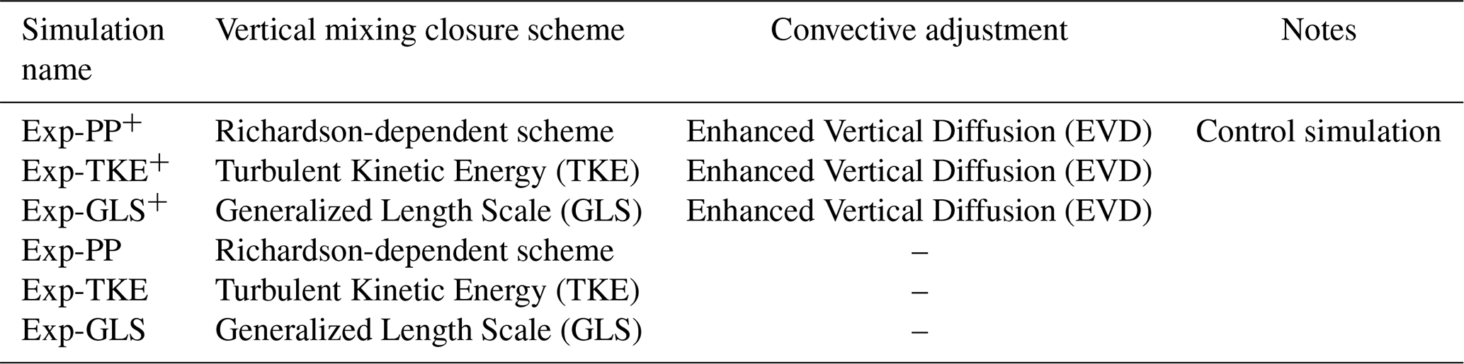
Three turbulence closure schemes are tested: the Richardson-number dependent parameterization (Pacanowski and Philander, 1981), the TKE closure scheme (Gaspar et al., 1990), and the GLS closure scheme (Umlauf and Burchard, 2003). These vertical mixing schemes are employed under two different convective setups: with and without the enhanced vertical diffusion parameterization typically used to mimic deep convection events. Therefore, the six simulations performed here differ only in the vertical mixing scheme and in whether convective adjustment is included. This experimental design allows us to assess the interplay between the choice of vertical mixing scheme and the effect of EVD, and to disentangle their individual and combined contributions to the representation of vertical mixing processes. It also enables us to evaluate how different turbulence closure schemes respond to the presence or absence of convective adjustment, and how this affects stratification, heat and salt distribution, and the overall vertical structure of the water column at basin and local scale.

Table 1 summarises the experiments. Our control run is defined as the simulation that employs the Richardson-number dependent vertical mixing scheme in combination with convective adjustment. Keeping convective adjustment active, we then replace the vertical mixing scheme with either TKE or GLS parameterisations. The remaining three experiments use the same three mixing schemes, but with convective adjustment disabled. In the experiments where convective adjustment is disabled, adaptive implicit vertical advection is activated to prevent local numerical instabilities (Shchepetkin, 2015; Madec and the NEMO System Team, 2023). All simulations are initialized from the same 31 December 2019 restart fields provided by the Mediterranean Forecasting System. These fields are analysis products that incorporate data assimilation of available observations, including satellite and in situ measurements. As a result, they provide an optimal representation of the Mediterranean Sea state at the start of the simulations, ensuring that all experiments begin from a physically realistic initial condition. The results presented hereafter are not affected by these initial conditions but rather reflect the changes in the vertical mixing schemes and convective adjustment listed in Table 1.

3 Results

3.1 Impact of the convective adjustment

The EVD parameterization exerts a strong control on the vertical structure of mixing. Figure 3 shows the eddy diffusivity coefficient along a zonal section at 37.5° N (as indicated in Fig. 1a) averaged over January 2021 for different mixing configurations. The presence of convective adjustment together with different mixing schemes (Fig. 3a, c, and e) tends to mask the differences among the various vertical mixing parameterisations resulting in a very similar eddy diffusivity pattern regardless of the chosen vertical mixing scheme. Given the different eddy diffusivity scales observed in the experiments with and without EVD (Fig. 3a, c and e versus Fig. 3b, d and f), it is clear that when EVD is active, the eddy diffusivity produced by the vertical mixing closure is largely overwritten by the EVD parameterization. In contrast, when convective adjustment is disabled (Fig. 3b, d and f), the vertical eddy diffusivity is determined solely by the mixing schemes and reveals more pronounced differences among schemes. Notably, the Richardson-dependent scheme (Fig. 3b) produces a relatively homogeneous increase in eddy diffusivity within the mixed layer, whereas the TKE (Fig. 3d) and GLS (Fig. 3f) schemes result in more heterogeneous structures. The magnitude of the vertical eddy diffusivity increases going from the Richardson-number dependent scheme (with maximum eddy diffusivity values on the order of 10⁻² m² s⁻¹) to the TKE and then to the GLS schemes (with maximum eddy diffusivity values on the order of 10⁻¹ m² s⁻¹). Moreover, when the EVD scheme is active, the maximum value of the vertical eddy diffusivity consistently occurs near the surface, while, when EVD is disabled, its maxima are typically found within the mid-depth of the mixed layer, which is more realistic due to the suppression of turbulent length at the top and the bottom of the mixed layer. This distinction underscores the role of EVD in favouring a surface-intensified mixing structure as opposed to the more symmetric and realistic profile observed in its absence, potentially impacting the MLD.

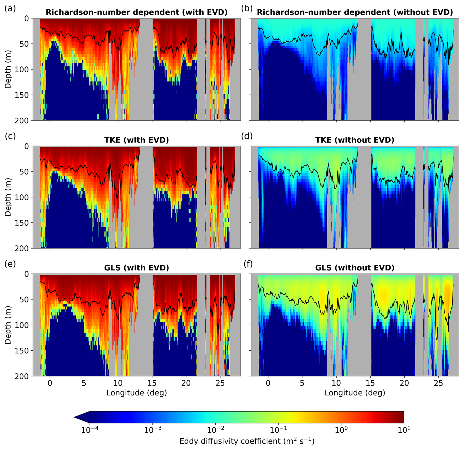
Figure 3 Vertical eddy diffusivity coefficient along the zonal section at 37.5° N (black line in Fig. 1a) averaged over January 2021 for different model configurations: (a) Richardson-dependent mixing scheme with EVD activated, and (b) without EVD activated; (c) TKE closure scheme with EVD activated, and (d) without EVD activated; (e) GLS scheme with EVD activated, and (f) without EVD activated. The black contours in each panel denote the depth of the mixed layer, while grey shading indicates land.

The EVD parameterisation is primarily intended to represent winter convection. However, convection-like vertical mixing occurs year-round, even outside the main winter season, and therefore the EVD parameterisation is active even in summer in some regions of the Mediterranean Sea. Figure 4 illustrates this by showing the maximum depth reached by the EVD on a summer day (1 July 2021) in the simulation using the Richardson-number dependent parameterization. White areas indicate the few regions where EVD is not applied on that day. Elsewhere the EVD is applied down to depths ranging from a few meters to several tens of meters reaching its maximum depth in the eastern Mediterranean Sea, and notably in the semi-permanent Ierapetra eddy region, located southeast of Crete within the Rhodes Gyre region (as defined in Fig. 1a). This activity is typically weaker and shallower than winter convection, but it still contributes to reshaping the vertical dynamics, as discussed in the following sections.

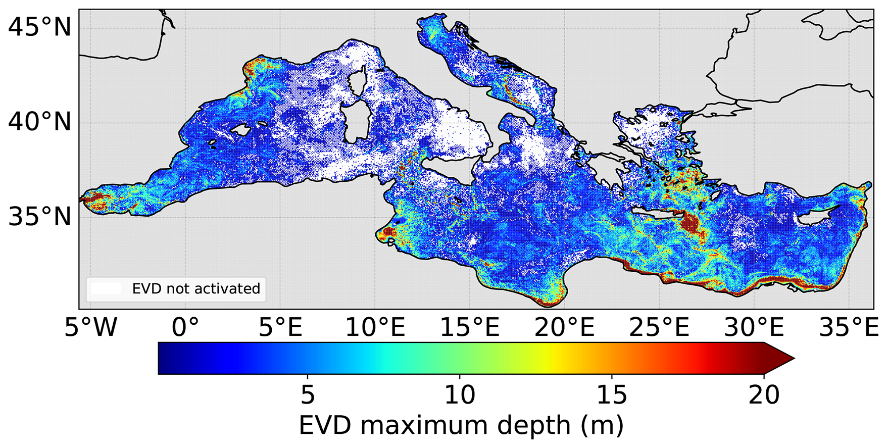
Figure 4 Map showing the maximum depth reached by the EVD parameterisation when activated in the control experiment (Exp-PP⁺ in Table 1) during a summer day (1 July 2021). White areas indicate regions where EVD is inactive.

3.2 Assessment at the basin scale

3.2.1 Impact on tracers

Among the different experiments (Table 1), the simulation using the Richardson-number dependent vertical mixing scheme combined with a convective adjustment (Exp-PP⁺) is taken as the control run. This configuration for the vertical mixing and convection corresponds to the current setup of the Mediterranean Forecasting System of the Copernicus Marine Service (Clementi et al., 2023).

To evaluate the performance of our control simulation and identify systematic deficiencies of the model, we compare the model outputs in terms of temperature and salinity with all available Argo data in 2020–2021 (Fig. 1a). We verified (not shown) that removing a spin-up period leads only to negligible differences and does not affect the results. Following the extensive literature on error decomposition for model validation (e.g., Willmott, 1981; Murphy, 1988, 1992; Oke et al., 2002; Oddo et al., 2022), we define four key statistical metrics, which provide complementary insights into model skills: the root mean squared error (RMSE), the unbiased root mean squared error (uRMSE), the mean bias (MB), and the cross-correlation coefficient (CC). For more details on their definition, see Appendix C. We compute these four metrics averaging on the entire basin and over the entire two-year period.

The temperature error profiles are shown in Fig. 5 as blue profiles. All metrics exhibit two pronounced decreases in model skill, one in the upper 50 m within the mixed layer and another between 200 and 600 m, corresponding to the Levantine Intermediate Waters (LIW) depth range (e.g., Bryden and Stommel, 1982; Robinson and Golnaraghi, 1993; Lascaratos et al., 1993; Taillandier et al., 2022). Within the mixed layer, RMSE and uRMSE peak at 25–30 m, corresponding to these two-year average MLD (30.8 m for observations and 28.3 m in the control simulation – dashed horizontal lines in Fig. 5). MB reaches its maximum around the middle of the MLD (about 15 m). CC exhibits a monotonic reduced decrease throughout the mixed layer, with a minimum below the yearly average MLD. A similar behaviour occurs within the LIW depth range, with a minimum in CC around 400 m, while RMSE, uRMSE and MB show their largest deviations slightly above, at approximately 350 m. Overall, this evidence indicates that errors are largest in the surface mixed layer but also reflect difficulties in representing intermediate water masses.

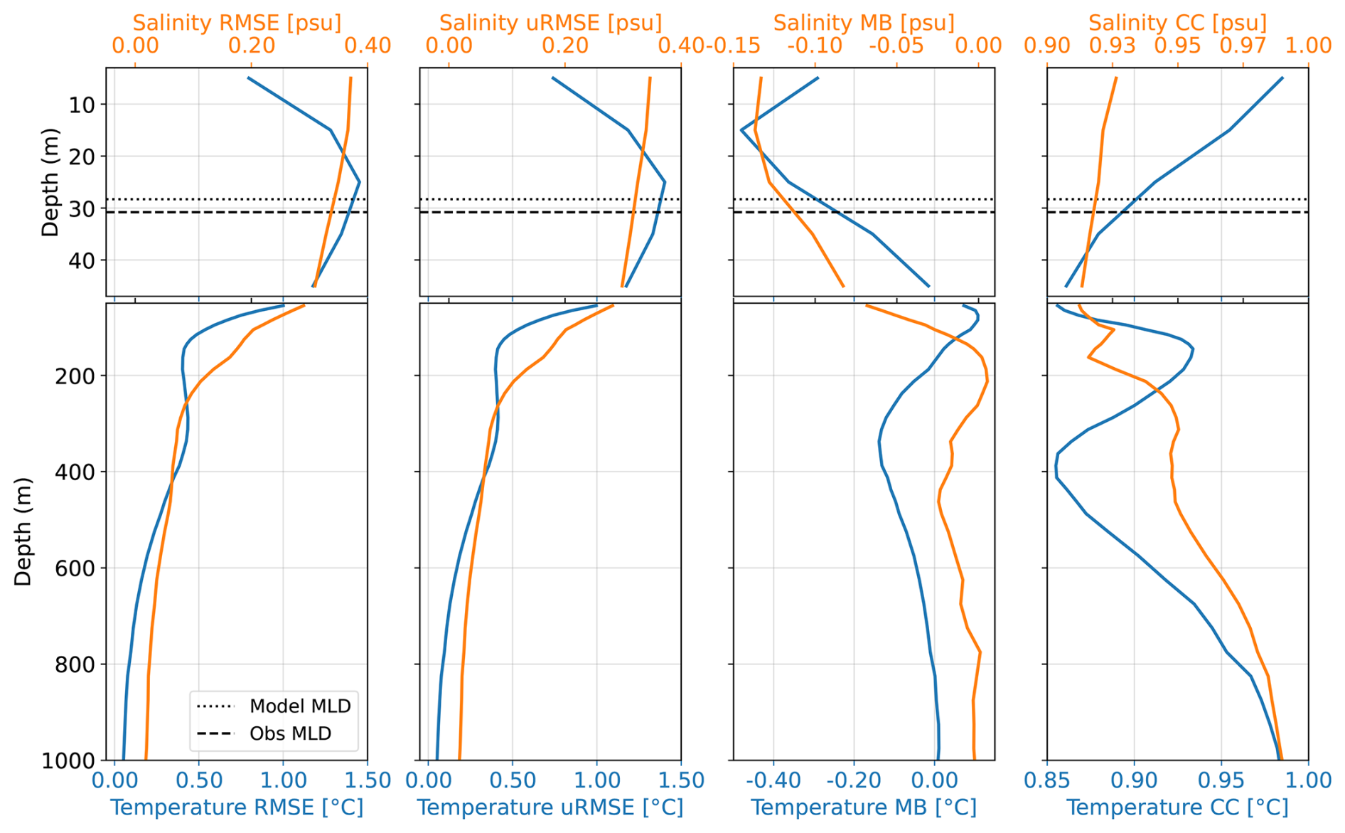
Figure 5 Basin-averaged temperature (blue) and salinity (orange) error profiles for 2020–2021 in the control simulation (Exp-PP⁺ in Table 1). Panels from left to right: root mean squared error (RMSE), unbiased root mean squared error (uRMSE), mean bias (MB), and cross-correlation coefficient (CC). The definitions of these metrices are in Appendix C. Dashed lines represent the two-year basin average values of the MLD for observations and control simulation.

The salinity error profiles (orange) in Fig. 5 show a distinct pattern compared to temperature. RMSE and uRMSE exhibit a single peak confined to the mixed layer, with no significant anomalies at the LIW depth range. Nevertheless, the MB highlights systematic fresh biases at both depth ranges, suggesting persistent model errors also in salinity in representing the LIW. We observe that the minimum salinity MB within the LIW depth range is found near the bottom of the LIW layer (about 500 m), while the minimum temperature MB occurs approximately at mid-depth within the layer (about 350 m). As for temperature, the CC decreases monotonically within the mixed layer; however, unlike temperature, it exhibits only a weak secondary minimum at LIW depths. These findings suggest that salinity shows smaller discrepancies than temperature with respect to observations in the representation of intermediate waters, while it also presents a discrepancy with the observation within the mixed layer.

As stated above, overall, for both salinity and temperature, the shape of the error at the basin scale suggests two main decreases of the model skills: the representation of the properties within the mixed layer and the intermediate water masses. The control simulation performs reasonably well in the deep region, while the more pronounced biases are within the mixed layer. These biases are likely related to the vertical mixing scheme, highlighting the need for a more realistic treatment of atmospheric energy input and vertical redistribution of momentum and buoyancy.

To assess the impact of the different closure schemes and the activation of the convective adjustment at the basin scale, we compare the metrices obtained for the other five simulations (simulation other than Exp-PP⁺ in Table 1) with these of the control run. Figures 6 and 7 show the basin-averaged error difference for temperature and salinity, respectively. For each experiment and each metric (Eqs. C1–C4), the error difference (err_diff) as a function of depth is computed as

$$\begin{array}{}\text{(1)}& {\mathrm{err}}_{\mathrm{diff}}={\mathrm{err}}_{\mathrm{mod}}\left(z\right)-{\mathrm{err}}_{\mathrm{CS}}\left(z\right)\end{array}$$

where err_CS(z) denotes the error of the control run (Exp-PP⁺, see Fig. 5), and err_mod(z) is the error associated with each model configuration (experiments other than Exp-PP⁺ in Table 1). Here, “err” generically denotes one of the four metrics (RMSE, uRMSE, MB, or CC) detailed in Appendix C. For the MB_diff metric, the absolute value of the mean bias is used for both the control run and the model experiments when computing MB_diff.

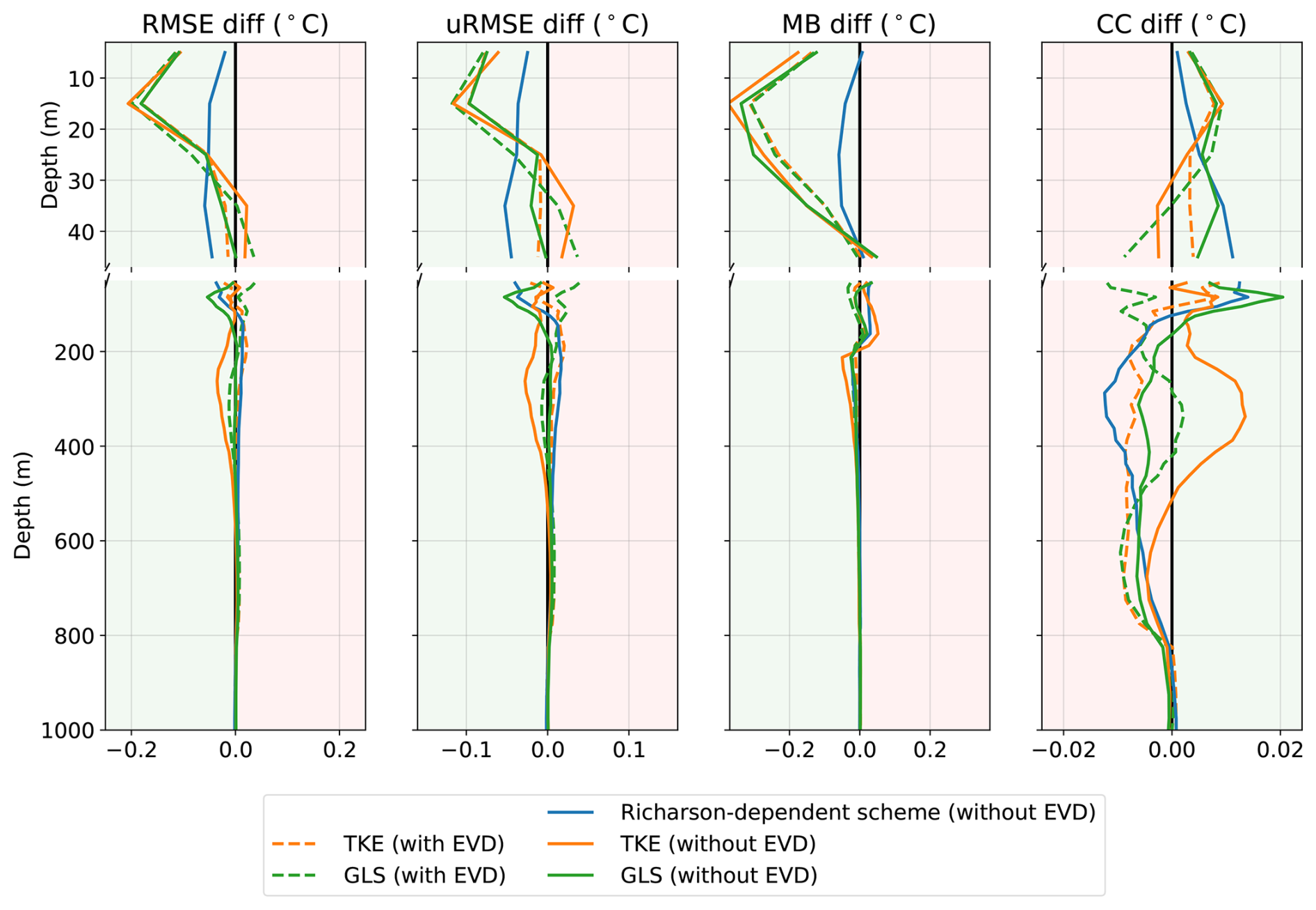
Figure 6 Temperature error difference (Eq. 1) with respect to the control simulation for the four metrics in Eqs. (C1)–(C4). Dashed lines indicate simulations with EVD and continuous lines without EVD. The transparent background color highlights regions of improvement (green) and worsening (red) compared to the control simulation.

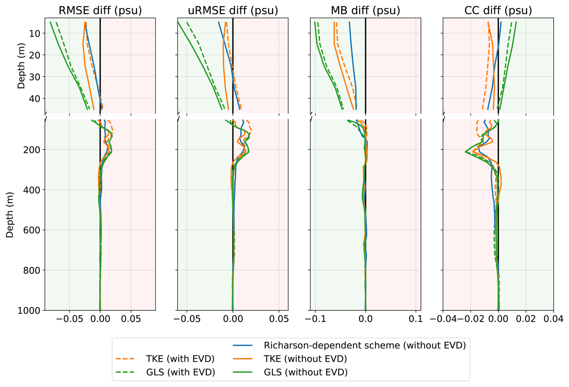
Figure 7 Salinity error difference (Eq. 1) with respect to the control simulation for the four metrics in Eqs. (C1)–(C4). Dashed lines indicate simulations with EVD and continuous lines without EVD. The transparent background colour highlights regions of improvement (green) and worsening (red) compared to the control simulation.

It should be noted that negative values of RMSE_diff, uRMSE_diff, and MB_diff indicate improvement, while positive values indicate deterioration. For CC_diff, the interpretation is reversed: higher values (closer to 1) denote improvement, whereas lower values (towards 0) denote deterioration. Accordingly, in Figs. 6 and 7 green and red backgrounds highlight regions of improvement and deterioration relative to the control simulation, respectively.

For temperature (Fig. 6), the error profiles indicate that the GLS closure scheme without convection parameterization (solid green line) provides the largest error reduction, expecially in terms of MB_diff, a result further confirmed by the CC_diff. The greatest improvement occurs within the mixed layer, mostly reflecting a reduction in systematic errors (MB_diff), while additional improvements at LIW depths are observed in terms of uRMSE_diff and CC_diff. Adding the convection parameterization to GLS (dashed green line) diminishes these gains at some depths, and mostly for MB_diff. The TKE mixing scheme exhibits intermediate skill: with or without EVD (orange lines), improvements are mostly confined to the mixed layer, while performance below this layer often deteriorates. The Richardson-dependent scheme without EVD (solid blue line) shows the smallest improvement within the mixed layer and a worsening in the LIW layer across all metrics. This behaviour is expected because the scheme estimates turbulence solely from the Richardson number (see Sect. 2.2.1 and Appendix A), that is from the balance between vertical shear and stratification (buoyancy) and does not include convective mixing. Consequently, it is expected that an additional parameterization would be required to properly represent convection.

For salinity (Fig. 7) in the absence of convective adjustment (solid lines), GLS is the only scheme showing improvements above 100 m for RMSE_diff, uRMSE_diff, CC_diff, and MB_diff. At the LIW depths, changes are minimal and a small degradation occurs for all experiments between about 100 and 200 m. The TKE and Richardson-number dependent schemes without EVD show smaller improvement in all metrics, particularly within the mixed layer, with the Richardson-number dependent scheme (solid blue line) performing worst, especially for CC_diff.

3.2.2 Representation of the mixed layer depth

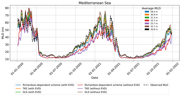
Given that the largest impact of the interplay between the mixing closure parameterisation and the convective adjustment occurs within the mixed layer, we also investigate how well the different schemes reproduce the MLD across the Mediterranean Sea. Figure 8 shows the time evolution of the MLD for the years 2020–2021, as computed from all available Argo temperature and salinity observations (black dashed line) and from model outputs (coloured lines) at the corresponding locations. Notably, for each day, model temperature and salinity profiles are first sampled at each Argo location. Density and MLD are then computed individually for each profile in both models and observations, and a basin average MLD is finally calculated.

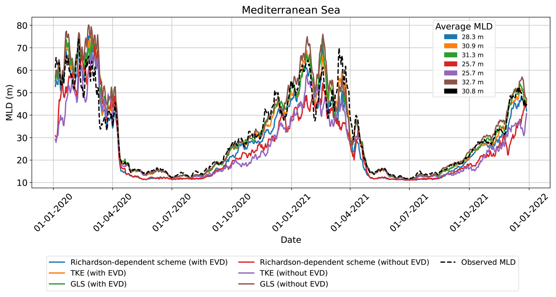
Figure 8 Time evolution of basin-averaged MLD for varying vertical mixing schemes, with and without convection parameterisation (configurations listed in Table 1). The black dashed line represents the MLD from Argo observations. A 7 d moving average has been applied to both model outputs and observations.

The MLD for both observations and model outputs is computed using the density threshold method, which identifies the depth at which the potential density increases by a fixed amount relative to a near-surface value. Specifically, here, the MLD is defined as the depth where the potential density exceeds that at 10 m by 0.01 kg m⁻³. With this definition, a minimum MLD of 10 m is imposed, as the reference density is taken at that depth. This approach, commonly used in oceanographic studies, provides a robust estimate of the mixed layer under both stratified and convective conditions (e.g., de Boyer Montégut et al., 2004).

The observed temporal evolution of the basin-averaged MLD over the period 2020–2021 oscillates around a temporal-spatial average value of 31 m and exhibits a pronounced seasonal cycle, with deepening during winter and shoaling in summer. On average, the MLD reaches its maximum around 70–80 m in winter (December to March), when surface cooling and intense wind forcing promote vertical convection and deep mixing. In spring, the increasing solar radiation and weakening winds lead to rapid surface warming and stratification, resulting in a marked shoaling of the MLD. By summer (June to September), the MLD stabilises at its shallowest levels, below 20 m, reflecting strong thermal stratification and limited vertical mixing. In autumn, cooling and more frequent wind events gradually deepen the MLD again, preparing the system for winter convection.

All simulations, colour-coded according to model configuration, reproduce this seasonal pattern, with winter maxima exceeding 70 m and summer minima around 15 m. However, significant differences in the MLD emerge while employing different vertical mixing schemes and varies also significantly depending on whether the EVD convection parameterisation is activated or not.

Simulations including EVD (blue, orange, and green lines) behave in a similar way and very close to the observations (black line). They occasionally show deeper (e.g. February–March 2020) or shallower (e.g. March 2021) winter MLDs and overall, they exhibit a good agreement in summer. With EVD activated, the two-year average MLD with TKE (30.9 m) and GLS (31.3 m) are very close to the observed one (30.8 m), while the Richardson-number dependent scheme tends to underestimate the MLD especially in summer (average of 28.3 m).

Simulations without EVD (red, purple, and brown lines) show distinct behaviours. The Richardson-dependent scheme (red line) produces the shallowest winter MLD and a low average MLD (average of 25.7 m), significantly underestimating observed deep mixing even in summer. The TKE scheme (purple line) tends to underestimate the MLD, both in winter and in summer. Although it performs better than the Richardson-number dependent scheme yet still fails to capture the basin-average maximum depths seen in observations (average MLD of 25.7 m). On the other hand, the GLS scheme (brown line) yields winter and summer MLDs closely aligned with observations, remaining in good agreement to them throughout the year. With the GLS, the average value of MLD without convective adjustment (32.7 m) is very close to the one obtained with convective adjustment included (31.3 m).

The GLS scheme without convective adjustment reproduces the observed deepening of the mixed layer, while the TKE and the Richardson-dependent scheme do not. This evidence demonstrates that this scheme does not need an additional external convection parameterisation to reproduce realistic mixed layer deepening. This may be attributed to the two-equation structure of the GLS (see Sect. 2.2.1 and Appendix A): the first equation evolves the turbulent kinetic energy over time, indicating where mixing is possible, while the second equation dynamically adjusts the turbulence length scale, controlling how deeply mixing penetrates. In contrast, the TKE scheme lacks dynamic depth control, and the Richardson-dependent scheme does not even include prognostic turbulent kinetic energy; in both cases, the penetration of convective mixing is limited. It is worth noting that, in the absence of explicit convective adjustment, the additional physics included in the TKE scheme compared to the Richardson-dependent formulation appears to have only a minor impact, likely because, at these scales, TKE still provides a relatively simplified representation of convective processes.

3.3 Assessment of water mass formation

The Mediterranean Sea hosts several key sites of deep and intermediate water formation, including the Gulf of Lion, the South Adriatic Sea, the Rhodes Gyre area and the Aegean Sea (e.g., Lascaratos et al., 1999; Simoncelli et al., 2018; Pinardi et al., 2019; Pinardi and Masetti, 2000; Pinardi et al., 2023). In these regions, vertical mixing and convection play a fundamental role in preconditioning and driving dense water formation processes by contributing to surface buoyancy loss and erosion of stratification (e.g., MEDOC Group, 1970; Schroeder et al., 2016). The intensity and vertical structure of turbulent mixing directly influence the transformation and ventilation of water masses, making its accurate representation essential for modelling the basin-scale thermohaline circulation (e.g., Simoncelli et al., 2018; Pinardi et al., 2019; Somot et al., 2006).

As case studies, to further investigate the impact of the interplay between different vertical mixing schemes and convective adjustment, we select one site of DWF (the South Adriatic Pit) and one site of both deep and intermediate water formation (the Rhodes Gyre region) and analyse them across the various model configurations during two selected time windows in 2021. We note that after more than one year of integration, although all six experiments are initialized from the same initial conditions, the six simulations have already had time to substantially diverge by the beginning of 2020. This divergence, driven solely by the different mixing and convective adjustment configurations (Sect. 2.3 and Table 1), encompasses not only differences in local vertical mixing, but also in the large-scale circulation, mesoscale structure and lateral advection. Consequently, while this section focuses on the behaviour of the schemes within two selected time windows in 2021, the results inherently reflect the prior evolution and memory of the system under each parameterization. This approach allows us to assess the resulting quasi-equilibrium state, accounting for how each scheme steers the model toward a distinct numerical and physical regime through its cumulative effects over time and its interplay with the convective adjustment parameterization. Therefore, our objective in this section is not to evaluate turbulence closure schemes in isolation, but rather to investigate their integrated impact in deep and intermediate water formation regions, within the general circulation of the Mediterranean Sea.

3.3.1 Deep water formation and intermediate water intrusion in the south Adriatic Pit

The South Adriatic Pit (defined as in Simoncelli et al. (2018) between longitudes 17–19° E and latitudes 41–42.5° N and shown in Fig. 1a) reaches a depth of 1200 m and is connected to the Eastern Mediterranean Basin through the Strait of Otranto. It is one of the principal sites of DWF in the Mediterranean Sea, where intense cooling and evaporation during winter – especially in February–March – induce strong density increases that drive dense water sinking and convective overturning (e.g., Wüst, 1961; Gačić et al., 2001; Manca et al., 2003). During these events, the MLD can deepen substantially, typically reaching between 600 and 800 m (e.g., Manca et al., 2003; Pinardi et al., 2023).

In Fig. 9 we show the temperature and salinity profiles as recorded by an Argo float (black dashed line) on 25 February 2021 in comparison with the modelled profiles at the same location for varying vertical mixing schemes and activating (dashed line) or deactivating (continuous line) the EVD. The location of the profile is shown in the insert of Fig. 9a. Argo observations show a nearly uniform layer in the upper ∼500 m, followed by a sharp gradient below. This inflection point corresponds to the MLD. Among the models in which EVD is active, the simplest Richardson-dependent scheme performs best, although it underestimates the MLD in the salinity profile of about 50 m. In this case, the GLS scheme underestimates the MLD in both temperature and salinity by about 100 m. In the absence of EVD, we observe a similar behaviour across different mixing scheme, with a broad inflection point corresponding to MLD around 500 m. To investigate how the various configurations of mixing and convection lead to the situation shown in Fig. 9, we examine the time evolution of the salinity field at this location up to the day of the profiles in Fig. 9. Salinity was chosen because it largely reflects the imprint of deep and intermediate water (Fig. 1d).

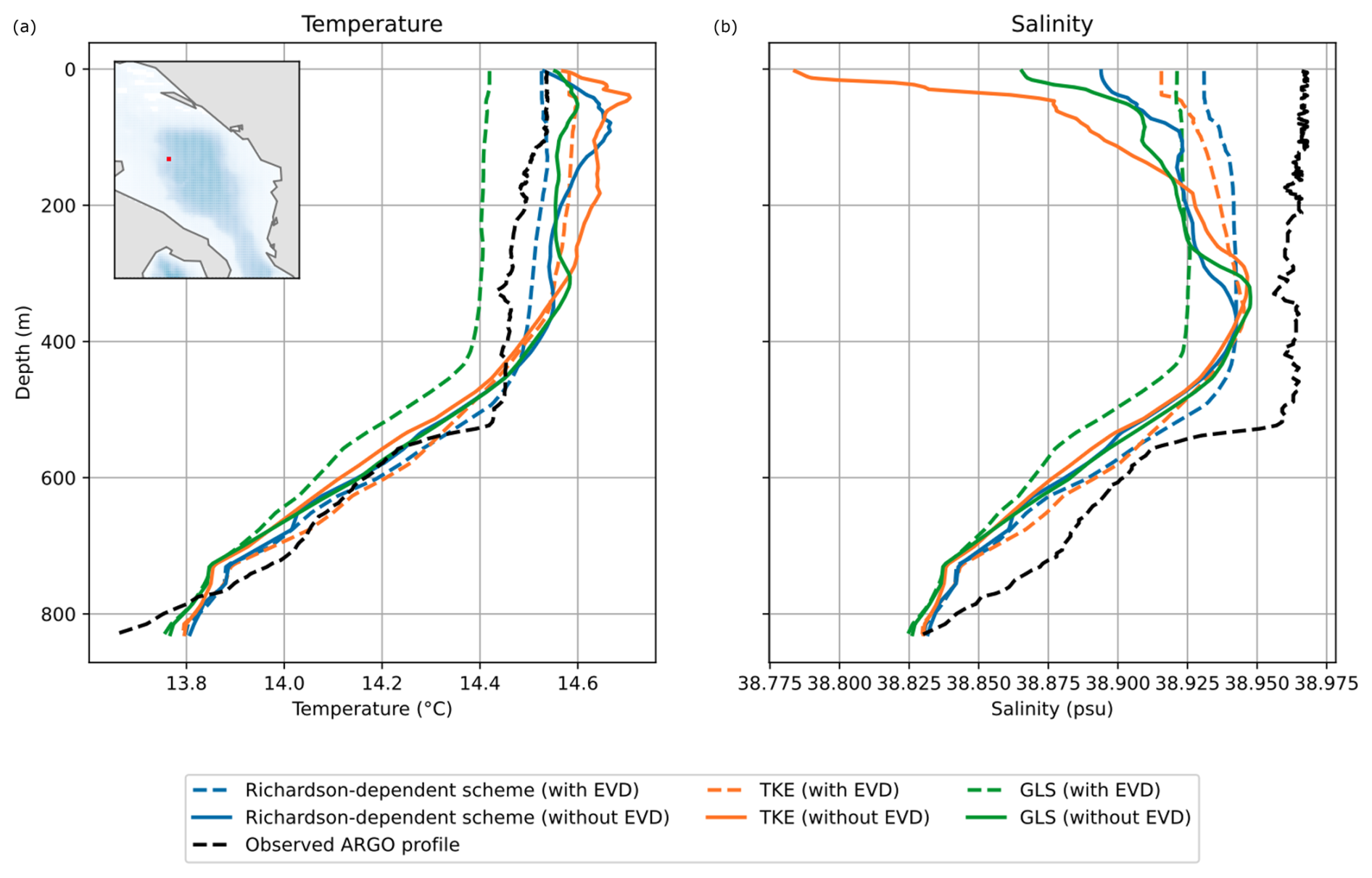
Figure 9 (a) Temperature and (b) salinity model profiles compared to observations (black dashed line) from an Argo float on 25 February 2021. Modelled profiles are color-coded by different vertical mixing schemes, with and without convective adjustment as indicated in the legend. The inset in the left panel shows the position of the Argo float.

In Fig. 10, we show the Hovmöller diagrams of salinity evolution at the site described above from 1 to 25 February 2021. The last day of each Hovmöller corresponds to the day of the profile shown in Fig. 9. The three panels on the left (Fig. 10a, c and e) show the salinity evolution for the models with EVD activated. The three panels on the right (Fig. 10b, d and f) correspond to the models with EVD deactivated. In the upper 100 m, the models with EVD activated show similar behaviour, with fresh water persisting until 13 February, whereas without EVD the models show large variability due to a different activation of mixing. In particular, the TKE scheme (Fig. 10d) maintains relatively fresh water up to 25 February, while the Richardson-number dependent scheme (Fig. 10b) and the GLS scheme (Fig. 10f) show increased salinity. However, the most notable differences occur at depth, between approximately 100 and 400 m, where a tongue of salty LIW gradually intrudes and a convective event, initially confined to the surface after 13 February, gradually deepens into intermediate layers. The contrast between simulations with and without EVD is substantial.

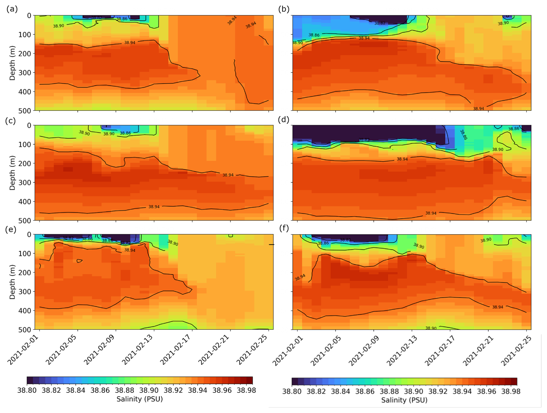
Figure 10 Hovmöller diagrams showing the temporal evolution of salinity at the location indicated in Fig. 9a (inset) from 1 to 25 February 2021 for different model configurations: (a) Richardson-dependent mixing scheme with EVD activated, and (b) without EVD activated; (c) TKE closure scheme with EVD activated, and (d) without EVD activated; (e) GLS scheme with EVD activated, and (f) without EVD activated. The last day in each panel corresponds to the day of the profile shown in Fig. 9.

In the presence of EVD, convection triggered after 13 February erodes the intruding LIW, so that the LIW is completely mixed thereafter. As discussed in Sects. 2.2.2 and 3.1, when the convective adjustment is applied, the vertical eddy diffusivity resulting from the mixing schemes, is abruptly replaced with a high constant value, disregarding the temporal evolution of the tracers. This is evident after 13 February regardless of the mixing scheme (Fig. 10a, c and e), with the salinity field homogenized across both time and depth. Consequently, convection parameterized though EVD does not account for prior stratification: the method is applied uniformly, effectively erasing pre-existing or intruding structure in the region.

Conversely, in the cases without EVD, the LIW persists up to 25 February. In particular, in the GLS scheme (Fig. 10f) the LIW gradually sinks to about 400 m due to its higher density (similarly to what shown in Fig. 1d), exhibiting a more realistic behaviour, whereas in the Richardson-number-dependent scheme (Fig. 10b) it drops abruptly, and in the TKE scheme (Fig. 10d) it remains at roughly the same depth. This behaviour is consistent with the formulation of the mixing schemes, which may have also produced, over the prior integration period, differences in lateral advection and mesoscale activity that contribute to the contrasting salinity structures. With the GLS scheme (Fig. 10f), which includes a prognostic equation for the mixing length (Sect. 2.2.1 and Appendix A), both the intensity and depth of convective events appear to be more realistically represented. On the other hand, with the TKE scheme (Fig. 10d), the convective intensity is similar, but the depth of the event is underestimated. For example, on 21 February, the salinity intrusion extends below 300 m with GLS, whereas with TKE the intrusion already begins at 200 m. In the Richardson-dependent formulation (Fig. 10b), the convective event is weaker and more abrupt, producing a less gradual penetration into deeper layers.

3.3.2 Deep and intermediate water formation in the Rhodes Gyre region

As an additional case study, we investigate the capability of the model to reproduce deep and intermediate water in the Rhodes Gyre region, defined here between longitudes 26.3–31° E and latitudes 33–36.1° N and shown in Fig. 1a. This region, located in the eastern Mediterranean Sea between Rhodes and Cyprus and extending southward into the open Levantine Sea, hosts the Rhodes Gyre and is the key site for the formation and initial spreading of the LIW. Relative to the domain defined by Simoncelli et al. (2018), here the region is expanded by 1° to the east and 1° to the south in order to better resolve the early spreading of the LIW. This water mass, characterised by high salinity and intermediate depth (approximately 200–500 m), begins spreading within the defined region and subsequently extends further across the Mediterranean Sea, influencing basin-scale thermohaline circulation (e.g., Lascaratos et al., 1993; Kubin et al., 2019; Pinardi et al., 2023).

In Fig. 11a, salinity observations from all available Argo floats in the Rhodes Gyre region between January and April 2021 are compiled and arranged to form a Hövmoller diagram. Water with salinity exceeding 39.2 psu is observed above 200 m until approximately mid-February, when a convective event forces the high-salinity layer downward, resulting in a deepening of the entire water column. The LIW, with salinities ranging from 38.95 to 39.05 psu (Lascaratos et al., 1993), descends from approximately 300 m to depth below 400 m.

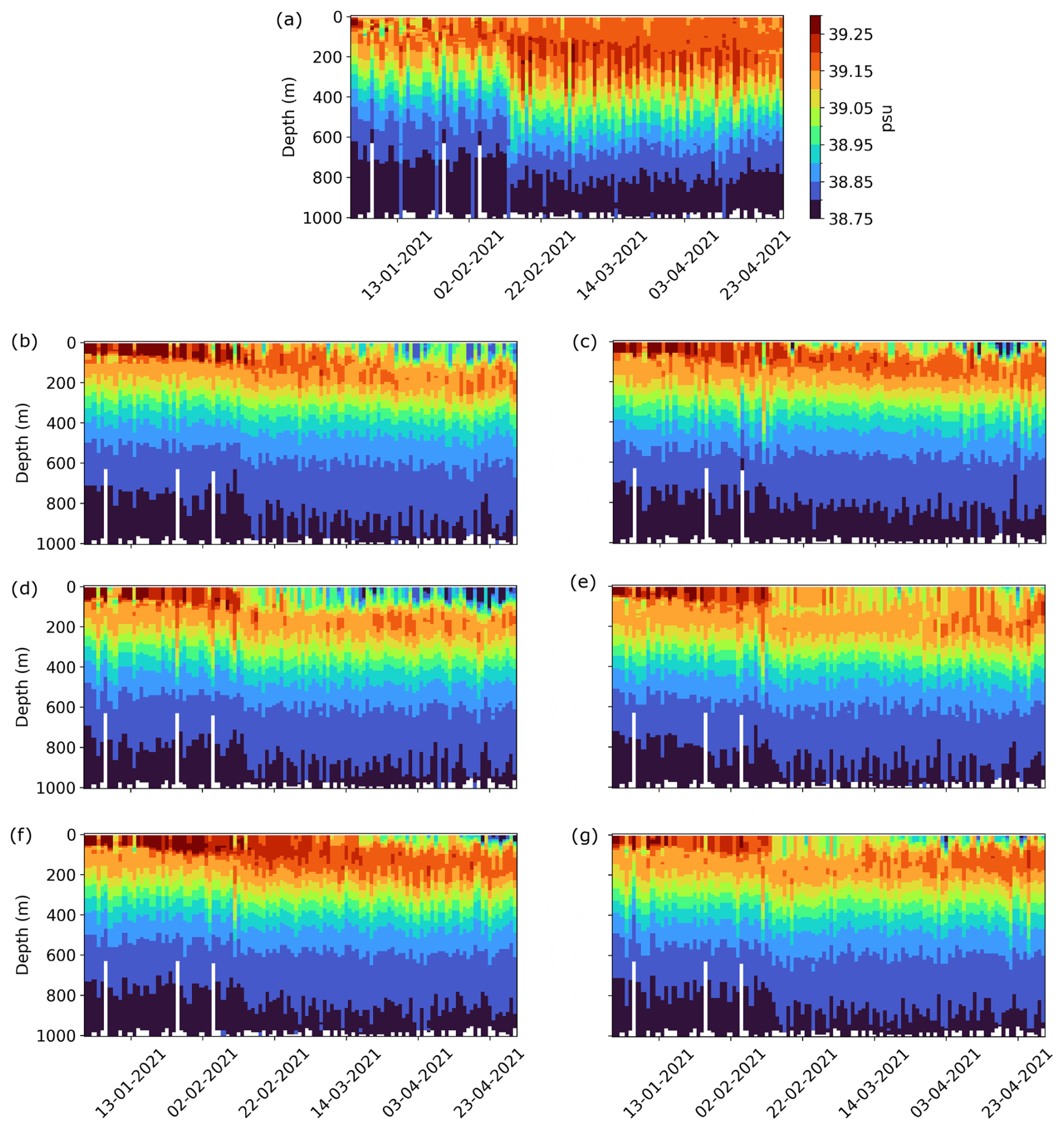
Figure 11 (a) Hovmöller diagram of salinity observations from available Argo floats in the Rhodes Gyre region (Fig. 1a) between January and April 2021. (b–g) Hovmöller diagrams of salinity for different vertical mixing schemes and convective adjustment settings: (b) Richardson-dependent mixing scheme with EVD activated, and (c) without EVD activated; (d) TKE closure scheme with EVD activated, and (e) without EVD activated; (f) GLS scheme with EVD activated, and (g) without EVD activated. All panels share the colour scale in panel (a).

In Fig. 11b–g we present Hovmöller diagrams of salinity for each model configuration. Overall, the model reproduces the observed stratification well and generally reach similar maximum salinity values, with some differences for varying mixing scheme and depending on the presence or absence of convective adjustment. As discussed above, the spread among configurations reflects not only the direct effect of local vertical mixing, but also differences in background circulation, mesoscale structure, and lateral advection accumulated over the prior integration period under each vertical mixing and convective adjustment setting (Table 1). In the upper 100 m, prior to the mid-February convective event, all models tend to overestimate salinity relative to observations, whereas after the event they generally produce fresher waters. At greater depths, model layers are generally narrower and more confined than in the observations, where post-convective mixing causes substantial vertical widening of the layer.

When EVD is applied (Fig. 11b, d and f), the convective event is weakly reproduced. The downward displacement of the water column is most evident in the TKE scheme (Fig. 11d), producing a deepening of approximately 100 m, whereas in the Richardson-dependent scheme (Fig. 11b) and GLS scheme (Fig. 11f), the column exhibits almost no abrupt shift, showing only gradual deepening over time. Overall, EVD suppresses the differences among the mixing schemes and results in a very similar salinity response to convection.

In the absence of EVD (Fig. 11c, e and g), the salinity response differs. With Richardson-dependent scheme (Fig. 11c), the behaviour is very similar to the case with EVD (Fig. 11b), with progressive deepening of the column without a sudden convective shift. This evidence reflects the fact that the Richardson-dependent scheme does not explicitly model convection but only increases mixing when shear dominates over buoyancy (Sect. 2.2.1). Consequently, convective events are weakly represented: the water column deepens gradually, and high-salinity layers remain confined and less vertically spread compared to observations or schemes that explicitly account for convection. By contrast, the TKE (Fig. 11e) and the GLS (Fig. 11g) schemes alone capture the mid-February convective event, producing a rapid downward displacement of the entire water column, with the GLS scheme better representing the intensity and extend of deepening due to its prognostic treatment of turbulent kinetic energy while simultaneously estimating a turbulence length scale.

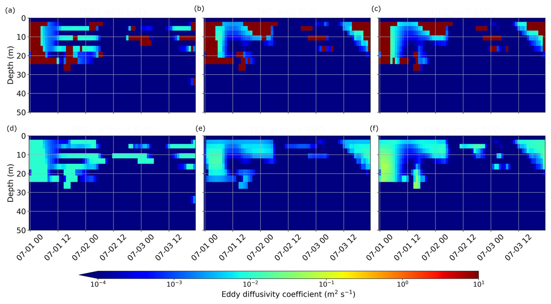
Figure 12 Hovmöller diagrams of the hourly eddy diffusivity coefficient at a site (27.5° E, 34.4° N) in the Rhodes Gyre region between 1 and 3 July 2021 (upper 50 m) for the six simulations with (a) Richardson-number dependent scheme with EVD, (b) TKE with EVD, (c) GLS with EVD, (d) Richardson-number dependent scheme without EVD, (e) TKE without EVD, (f) GLS without EVD.

3.4 Assessment of the nighttime summer convection daily cycle

In summer, the upper layers of the ocean exhibit a pronounced diurnal cycle in temperature, primarily controlled by the alternation of solar heating during the day and cooling processes at night. Surface waters warm under strong solar radiation, leading to a shallow, well-defined thermal stratification, while nocturnal cooling can erode this stratification. These processes occur within the mixed layer, which remains relatively shallow, as the rapid diurnal cycle of formation and destructing does not allow it sufficient time to deepen and night cooling is not as strong as in winter. Consequently, these processes are expected to be strongly influenced by the selected mixing scheme and the presence of a convective adjustment, which can significantly modify both the intensity of the heating and the depth of the near-surface warm layer. As shown in Fig. 4, the EVD during a summer day remains typically around an average of a few meters, but in certain areas – such as the Ierapetra semi-permanent gyre area within the Rhodes Gyre region as defined in the previous section – it can reach tens of meters.

The simulations in Table 1 were performed again starting from 1 July 2021 for three days, producing hourly outputs. The same initial conditions were used for all simulations, with the goal of monitoring how the mixing closure scheme and the presence of convective adjustment influence the daily cycle. As a case study, we focus on a site (27.5° E, 34.4° N) within the Rhodes Gyre region where the EVD reaches its greatest activation depth during summer (Fig. 4).

Figure 12 shows Hovmöller diagrams of the eddy diffusivity coefficient at that location in the upper 50 m for the six simulations. The upper panels correspond to the three simulations with EVD activated, whereas the lower panels show the cases without EVD. In general summer convective events tend to occur during nighttime because of surface cooling associated with absence of solar heating and extend along the water column within the upper few tens of meters (∼30 m in Fig. 12). As already observed in Fig. 3, when EVD is activated, the eddy diffusivity coefficient produced by the vertical mixing scheme is largely overwritten by the EVD parameterization (note the three-order-of-magnitude difference between the upper and lower panels in Fig. 12), resulting in similar mixing patterns regardless of the turbulence closure scheme used. The background eddy diffusivity produced by each mixing scheme remains visible beneath the EVD signal, albeit approximately two-to-three orders of magnitude lower.

In contrast, when EVD is not applied (bottom panels in Fig. 12), the representation of convection differs substantially among the three closure schemes. The Richardson-number dependent scheme produces weak but nearly persistent convective activity that remains present even during daytime. The TKE and GLS schemes instead exhibit a more intermittent pattern of convection, with events occurring less frequently and the strongest one during nighttime. Convective events simulated with the TKE scheme are generally weaker than these produced by the GLS scheme and tend to extend less deeply in the water column.

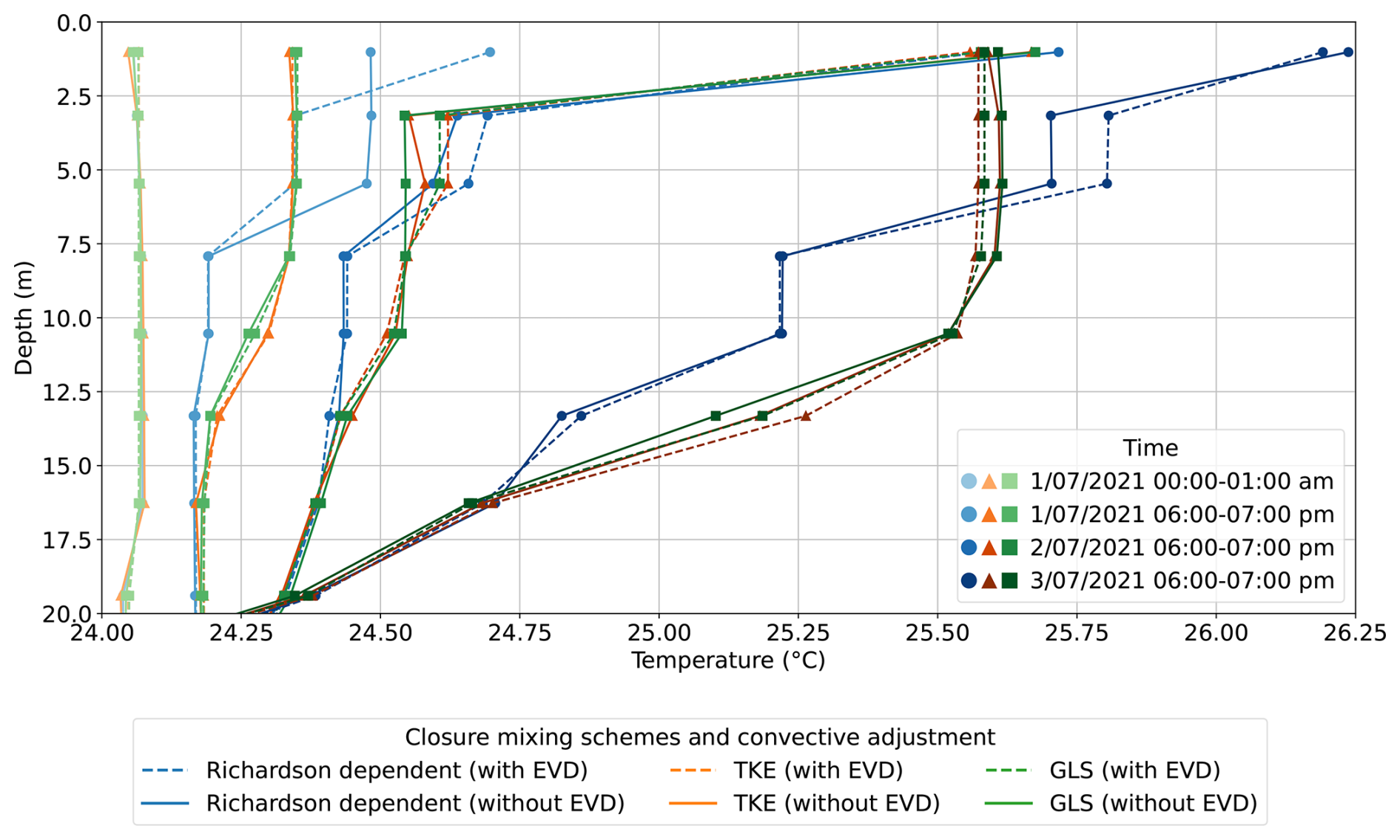
Figure 13 Temperature profiles at a site (27.5° E, 34.4° N) in the Rhodes Gyre region at different times of the day (see legend in the inset) and for different closure schemes and convective adjustment settings (see bottom legend).

For example, during the night of 1 July 2021, a convective event reaching approximately 25 m depth occurs in all simulations. In three cases with EVD (upper panels in Fig. 12), this event is represented very similarly and homogeneously throughout the upper 25 m, whereas without EVD (lower panel in Fig. 12) its amplitude and vertical structure differ substantially among the three closure schemes. In the Richardson-number dependent case, it appears as a relatively weak and vertically homogeneous event down to 25 m. In the TKE simulation, it is confined between about 10 and 20 m, with a peak around 15 m. In contrast, the GLS scheme produces a much stronger event, extending all the way down to 25 m.

These differences in the representation of summer convection, as seen in Fig. 12, both in terms of amplitude and vertical distribution along the water column, have a direct impact on the temperature field. In particular, the variability in convective activity simulated by the different turbulence closure schemes, and the homogenizing effect of EVD, translates into notable differences in the upper-ocean temperature structure. Figure 13 shows the temperature profiles at that site during the same three days and at different times of the day.

The first profiles (lightest colours) show that at the beginning – on 1 July 2021, between midnight and 01:00 UTC – the temperature profiles are well mixed and very similar to each other, with differences that are barely distinguishable, and are not yet influenced by the vertical mixing schemes or convective adjustment. Later the same day – between 18:00 and 19:00 UTC – we observe that, while the simulations with TKE (orange) and GLS (green) behave in a similar way both with and without convective adjustment, the Richardson-number-dependent scheme (blue) is strongly influenced by the presence or the absence of EVD. In fact, in the case of TKE and GLS, the simulations without EVD (solid lines) produce temperature profiles that are only slightly different than those with EVD (dashed lines). By contrast, the Richardson-number dependent scheme without EVD (solid blue line) yields a nearly uniform temperature in the first 5 m, followed by a gradual decrease with depth. With EVD (dashed blue line) the profile is reversed, showing a surface and deep gradient separated by an intermediate quasi-homogeneous layer.

In the following two days (2 and 3 July 2021, both at 18:00–19:00 UTC) the difference between the Richardson-number dependent scheme and the other two schemes increases in both profile shape and amplitude, reaching a sea surface temperature (SST) difference larger than 0.5 °C on 3 July. Moreover, the simulations with TKE and GLS exhibit only minor differences – on the order of ∼0.1 °C around 15 m depth – arising from slightly different convective patterns in terms of amplitude and vertical extend (Fig. 12e and f). In contrast, the Richardson-number dependent scheme shows much larger discrepancies, especially near the surface, due to the substantially different convective patterns (Fig. 12d).

4 Discussion and conclusions

Physics-based turbulence closure schemes can represent convective mixing in principle, but at typical model resolution they may underestimate the rate of instability removal. For this reason, convective adjustment is often applied as a numerical parameterization to rapidly stabilize the water column and mimic the fast overturning associated with unresolved convective events. In this work, we investigated how the combined effect of three vertical mixing schemes – Richardson-number dependent, TKE, and GLS closure schemes – and an external convective adjustment (EVD) affects the performance of a regional ocean circulation model of the Mediterranean Sea. We analysed the model outputs in relation to the physics of vertical mixing represented by the different schemes and assessed the advantages and drawbacks of applying an external convective parameterization alongside each of them.

The results first confirm what is known in the literature: the explicit representation of convection through enhanced vertical diffusion is crucial for simple schemes such as Richardson-number dependent closures, which lack an explicit formulation of convection and only reduce density gradient by enhancing vertical mixing in unstable layers. On the other hand, our results indicate that for more physically based schemes, the inclusion of a convective adjustment should be handled with care, as its application can be redundant or even degrade model performance. For the TKE scheme, we found that the inclusion of EVD can be beneficial in some cases. The TKE scheme has a single prognostic equation for turbulent kinetic energy, while the turbulent mixing length is defined diagnostically, and treats convection prognostically through the calculation of the turbulent kinetic energy; as a result, it often represents the intensity of convection well, but underestimates the penetration depth of convective events. In contrast, the GLS scheme, which treats convection prognostically through the calculation of both enhanced turbulent kinetic energy and turbulent mixing length, is generally better able to simulate both the penetration depth and the intensity of convective processes on its own. Therefore, with the GLS scheme, the convective adjustment is redundant and can often degrade the model's skill. These observations are confirmed both at basin scale and in deep and intermediate water formation regions.

At the basin scale, statistical metrics on temperature and salinity show that the GLS scheme performs best, followed by TKE and the Richardson-number dependent scheme. The inclusion of EVD makes little difference overall. In particular, we observed a more consistent improvement with GLS without EVD across all metrics and over a larger range of depths. The largest impact of including or excluding EVD at the basin scale is observed on the MLD. For both the Richardson-number dependent scheme and the TKE schemes, only the addition of the convective adjustment allows the model to reproduce the observed temporal evolution of the average MLD across the basin. This is because EVD compensates for mixing physical processes in these schemes: either the full convective overturning in the Richardson-number dependent scheme or the prognostic evaluation of the mixing length in TKE, which controls the convection penetration depth. In contrast, the GLS scheme, thanks to its prognostic treatment of both TKE and mixing length, is able to reproduce the observed basin-average MLD over time, including the MLD seasonal variability, without requiring an external convective parameterization.

In DWF areas, such as the south Adriatic Pit, where convective processes play a central role during dense water formation events, we observe that both the choice of mixing scheme and the inclusion of the convective adjustment play a major role in the development of deep water and the intrusion of intermediate water from the Levantine basin. Notably, the inclusion of EVD, with its abrupt and strong increase in vertical eddy diffusivity when unstable layers are present, does not account for previous states or the coherent temporal evolution of the water column: when applied, EVD disrupts pre-existing or intruding structures over time. The different mixing schemes without an external convective adjustment reproduce convection in distinct ways, and a similar behaviour is observed in the Rhodes Gyre region. The Richardson-number dependent scheme produces an abrupt but weak homogenization of the layers affected by surface convection, resulting in less gradual penetration into deeper layers and a partial removal of the intruding LIW. The TKE scheme reproduces convection with a smoother intensity transition compared to the Richardson-number dependent scheme, showing less abrupt effects on salinity. However, the penetration depth in the TKE scheme remains limited, without significant sinking of denser waters, due to the lack of a prognostic control on the penetration depth. In contrast, the GLS scheme more accurately represents both the intensity and penetration depth of convective events, allowing for a smooth sinking of the LIW.

Focusing on nighttime convection during summer, analysed at an hourly timescale, we observe how the nighttime convective adjustment, combined with different vertical mixing schemes, shapes the diurnal evolution of temperature. The three vertical mixing schemes represent summer convection differently: the TKE and GLS schemes largely capture the night-and-day differentiation, with GLS producing homogeneous, strong mixing that penetrates deeper. In contrast, the Richardson-number dependent scheme increases mixing weakly but almost continuously, even during daytime showing almost no day-night contrast. Temperature profiles using the Richardson-number dependent scheme differ noticeably from the other closure schemes, and after three days, the SST reaches a value roughly 0.5 °C higher.

In summary, across all temporal and spatial scales, our results highlight the crucial role of two key features in vertical mixing schemes. First, prognostic treatment of turbulent kinetic energy (as in the TKE and GLS schemes) is essential to accurately reproduce the intensity of overturning convection, retain memory of priori processes and ensure smooth transitions at a site, preserve pre-existing structures as well as the day-night alternation during summer convection. Second, a prognostic additional equation for the mixing length (as in the GLS scheme), rather than a fixed value as in TKE, is necessary to correctly represent the penetration depth of convective processes and to achieve the most accurate representation of the mixed layer depth. The inclusion of a convective adjustment to compensate for the lack of these features only partially addresses the deficiencies, as external convective adjustment are not embedded within the general framework and do not evolve prognostically.

These findings underscore how critical it is, in regional ocean modelling, to align appropriately the mixing closure and convection parameterisations. More broadly, these results highlight that careful choice of a combination of subgrid-scale parameterizations is essential to reliably simulate key oceanographic features and improve model interpretability in regional applications. Future work could extend this analysis to longer-term simulations and the effect of additional subgrid-scale processes – such as internal waves, eddy formation, and horizontal mixing – in order to further improve model realism and predictive skill. More broadly, our results highlight how the representation of vertical mixing can strongly influence deep and intermediate water formation and properties, with potential implications for regional ocean modelling in other basins with characteristics similar to the Mediterranean Sea. Comparable processes occur in other semi-enclosed or marginal basins, where dense water formation and vertical mixing play a key role in shaping water mass properties. Examples include the Black Sea and the Baltic Sea, as well as convection sites in other marginal seas. In these environments, the choice of vertical mixing parameterization may similarly affect the overall water mass structure in regional ocean models.

Appendix A

This appendix briefly summarizes the main equations of the three vertical mixing schemes used in this study, outlining how the eddy viscosity coefficient A^vm and diffusivity coefficient A^vT are determined for each scheme. We note that the eddy diffusivity coefficient for temperature, A^vT, is assumed to be equal to that for salinity: A^vS≡A^vT.

A1 Richardson-number dependent mixing scheme

The first closure scheme used here is based on the Richardson number – dependent formulation originally proposed by Pacanowski and Philander (1981), where the vertical eddy viscosity and diffusivity are parametrized as

$$\begin{array}{}\text{(A1)}& {\displaystyle }& {\displaystyle }{A}^{\mathrm{vm}}={\displaystyle \frac{A_{\mathrm{ric}}^{\mathrm{vm}}}{{\left(\mathrm{1}+\mathit{\alpha }{R}_i\right)}^n}}+A_{\mathrm{b}}^{\mathrm{vm}}\text{(A2)}& {\displaystyle }& {\displaystyle }{A}^{\mathrm{vT}}={\displaystyle \frac{A^{\mathrm{vm}}}{\left(\mathrm{1}+\mathit{\alpha }{R}_i\right)}}+A_{\mathrm{b}}^{\mathrm{vT}}\end{array}$$

where $R_i=\frac{N^{\mathrm{2}}}{(\partial U_{\mathrm{h}}{)}^{\mathrm{2}}}$ denotes the Richardson number, defined as the ratio between stratification (represented by the squared Brunt-Väisälä frequency, N²) and vertical shear (∂U_h)². The parameter $A_{\mathrm{ric}}^{\mathrm{vm}}$ represents the maximum value of the eddy viscosity coefficient reached when R_i<0; α and n are constant parameters. The additive terms $A_{\mathrm{b}}^{\mathrm{vm}}$ and $A_{\mathrm{b}}^{\mathrm{vT}}$ are background values that ensure a minimum level of vertical mixing even under stable conditions. For further details, see Pacanowski and Philander (1981) for the theoretical framework and Madec and the NEMO System Team (2023) for the practical implementation in NEMO.

A2 Turbulent Kinetic Energy (TKE) vertical mixing scheme

The TKE vertical mixing scheme solves a prognostic equation for the turbulent kinetic energy k, while assuming a diagnostic closure for the turbulent length scale l_k. The TKE equation is written as

$$\begin{array}{}\text{(A3)}& {\displaystyle \frac{\partial k}{\partial t}}=A^{\mathrm{vm}}{\left({\displaystyle \frac{\partial U_{\mathrm{h}}}{\partial z}}\right)}^{\mathrm{2}}-A^{\mathrm{vT}}{N}^{\mathrm{2}}+{\displaystyle \frac{\partial }{\partial z}}\left(A^{\mathrm{vm}}{\displaystyle \frac{\partial k}{\partial z}}\right)-C_{\mathit{ϵ}}{\displaystyle \frac{k^{\mathrm{3}/\mathrm{2}}}{l_{\mathit{ϵ}}}}\end{array}$$

where U_h is the horizontal velocity, N² is squared Brunt-Väisälä frequency, C_ϵ is a constant and l_ϵ is the dissipative length scale. On the right side of Eq. (A3), the four terms represent the main physical processes associated with vertical mixing. From left to right: shear production, stratification (or buoyancy) destruction, TKE diffusion and Kolmogorov dissipation (Kolmogorov, 1942). Vertical mixing coefficients are then computed as:

$$\begin{array}{}\text{(A4)}& {\displaystyle }& {\displaystyle }{A}^{\mathrm{vm}}=C_k{l}_k\sqrt{k}\text{(A5)}& {\displaystyle }& {\displaystyle }{A}^{\mathrm{vT}}={\displaystyle \frac{A^{\mathrm{vm}}}{P_{\mathrm{rt}}}}\end{array}$$

where l_k is the mixing length scale, C_k is a model constant, and P_rt is the Prandtl number. The turbulent mixing length l_k is computed diagnostically and its value is constrained by stratification (typically $l_k=l_{\mathit{ϵ}}=\sqrt{\mathrm{2}k}/N$, with additional operational caps imposed). For further details, see Gaspar et al. (1990) for the theoretical framework and Madec and the NEMO System Team (2023) for the practical implementation in NEMO.

A3 Generalized Length Scale (GLS) vertical mixing scheme

The GLS vertical mixing schemes solves two prognostic equations, one for the turbulent kinetic energy k and one for the generic length scale ψ. The evolution of the turbulent kinetic energy is governed by

$$\begin{array}{}\text{(A6)}& {\displaystyle \frac{\partial k}{\partial t}}={\displaystyle \frac{A^{\mathrm{vm}}}{{\mathit{\sigma }}_{\mathrm{e}}}}{\left({\displaystyle \frac{\partial U_{\mathrm{h}}}{\partial z}}\right)}^{\mathrm{2}}-A^{\mathrm{vT}}{N}^{\mathrm{2}}+{\displaystyle \frac{\partial }{\partial z}}\left(A^{\mathrm{vm}}{\displaystyle \frac{\partial k}{\partial z}}\right)-C_{\mathrm{0}\mathit{\mu }}{\displaystyle \frac{k^{\mathrm{3}/\mathrm{2}}}{l_{\mathit{ϵ}}}}.\end{array}$$

The equation is coupled with a prognostic equation for the generic length scale:

$$\begin{array}{}\text{(A7)}& \begin{array}{rl}{\displaystyle \frac{\partial \mathit{\psi }}{\partial t}}& ={\displaystyle \frac{\mathit{\psi }}{e}}\left\{{\displaystyle \frac{C_{\mathrm{1}}{A}^{\mathrm{vm}}}{{\mathit{\sigma }}_{\mathit{\psi }}}}{\left({\displaystyle \frac{\partial U_{\mathrm{h}}}{\partial z}}\right)}^{\mathrm{2}}-C_{\mathrm{3}}{A}^{\mathrm{vT}}{N}^{\mathrm{2}}\right.\\ & \left.-C_{\mathrm{2}}{C}_{\mathrm{0}\mathit{\mu }}{\displaystyle \frac{k^{\mathrm{3}/\mathrm{2}}}{l_{\mathit{ϵ}}}}{F}_{\mathrm{wall}}\right\}+{\displaystyle \frac{\partial }{\partial z}}\left(A^{\mathrm{vm}}{\displaystyle \frac{\partial \mathit{\psi }}{\partial z}}\right).\end{array}\end{array}$$

Here, F_wall denotes the wall function and C₁, C₂, C₃, σ_k and σ_ψ are constants that depends on the choice of the turbulent model. C_0μ is also a constant. The wall function is only needed in the Mellor-Yamada model.

The eddy viscosity and diffusivity coefficients are then computed from the turbulent kinetic energy and mixing length:

$$\begin{array}{}\text{(A8)}& {\displaystyle }& {\displaystyle }{A}^{\mathrm{vm}}=C_{\mathit{\mu }}{l}_k\sqrt{k}\text{(A9)}& {\displaystyle }& {\displaystyle }{A}^{\mathrm{vT}}=C_{{\mathit{\mu }}^{\prime }}{l}_k\sqrt{k}\end{array}$$

where C_μ and $C_{{\mathit{\mu }}^{\prime }}$ are the stability functions. The constant C_0μ depends on the choice of the stability functions. For further details, see Burchard and Bolding (2001) for the theoretical framework and Madec and the NEMO System Team (2023) for the practical implementation in NEMO.

Appendix B

In this appendix, we present the relevant portion of the namelist to be given as input to NEMO (version 4.2) corresponding to the three vertical mixing schemes used in this study. One table is provided for each scheme: Table B1 refers to the Richardson-number dependent schemes (Pacanowski and Philander, 1981), Table B2 to the TKE closure scheme (Gaspar et al., 1990) and Table B3 to the GLS closure scheme (Burchard and Bolding, 2001).

Table B1 NEMO namelist parameters of the Richardson-number dependent vertical mixing scheme.

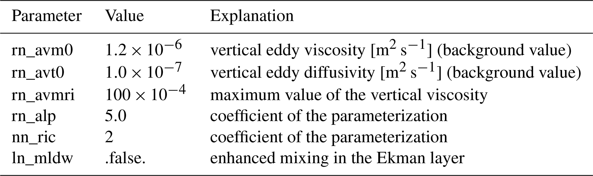
Table B2 NEMO namelist parameters of the Turbulent Kinetic Energy (TKE) vertical mixing scheme.

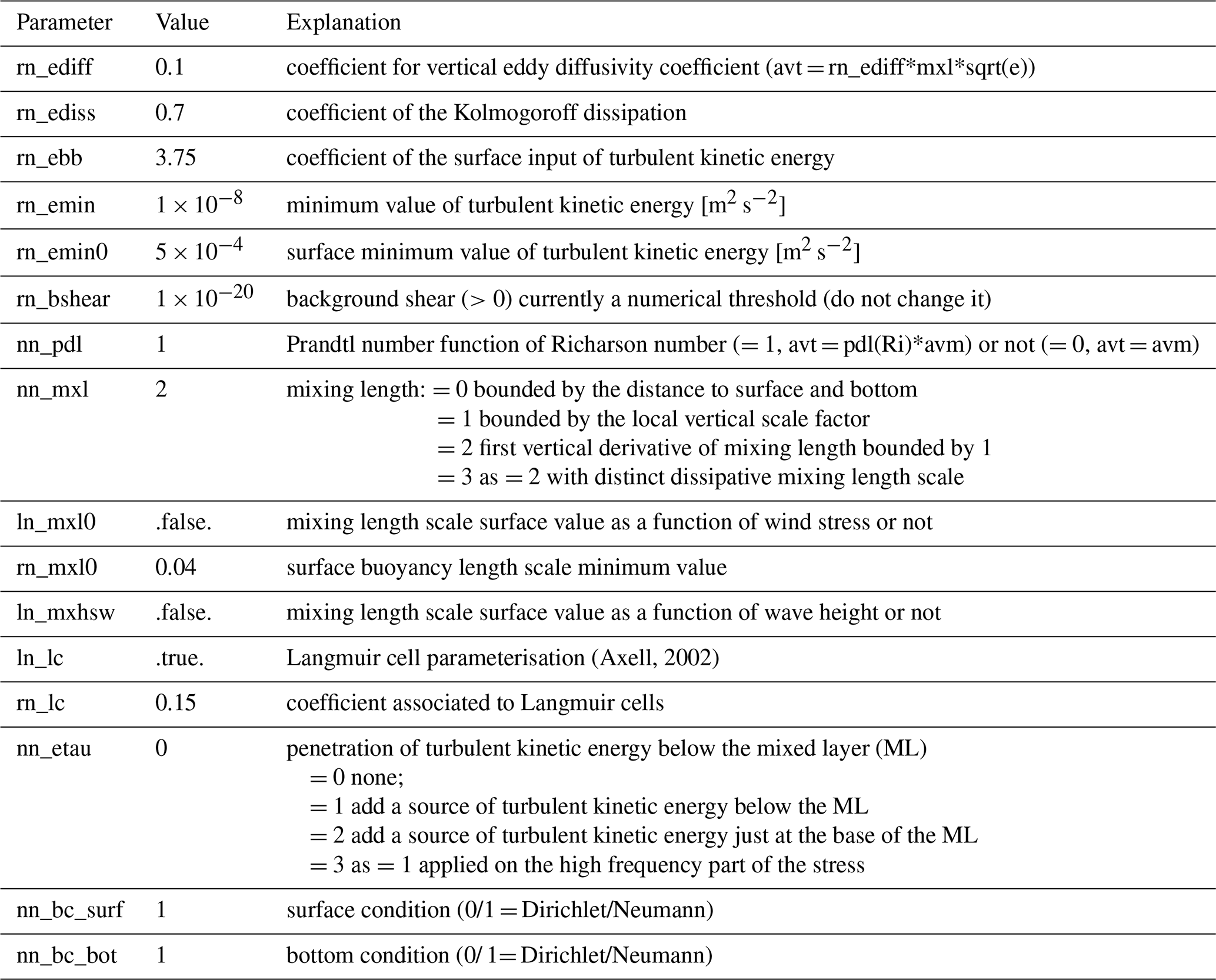
Table B3 NEMO namelist parameters of the Generalized Length Scale (GLS) vertical mixing scheme.

Appendix C

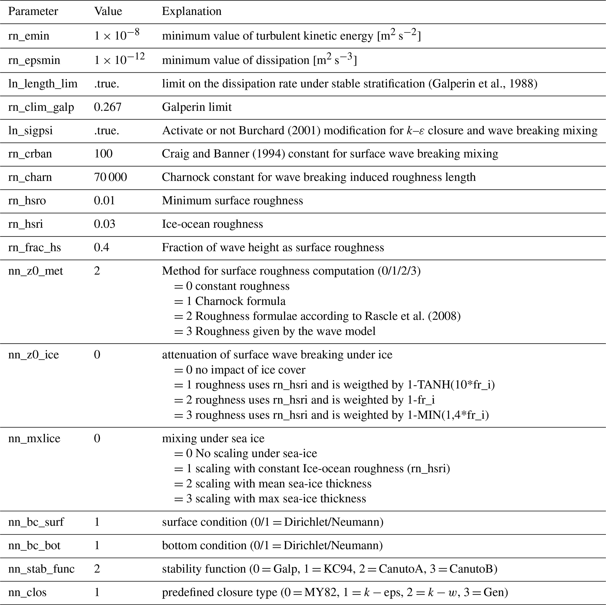
Throughput this paper, we define four statistics metrics (e.g., Willmott, 1981; Murphy, 1988, 1992; Oke et al., 2002, Oddo et al., 2022): the root mean squared error (RMSE), the unbiased root mean squared error (uRMSE), the mean bias (MB), and cross-correlation coefficient (CC). We denote $\stackrel{\mathrm{‾}}{o}$ and $\stackrel{\mathrm{‾}}{m}$ as the mean values of observations (o) and model data (m), N is the total number of observation-model pairs, and σ represents the standard deviation. The metrics are computed as follows.

The root mean squared error (RMSE), which combines both systematic and random errors into a single measure of overall discrepancy:

$$\begin{array}{}\text{(C1)}& \mathrm{RMSE}=\sqrt{{\displaystyle \frac{\mathrm{1}}{N}}\sum _{i=\mathrm{1}}^N{\left(m_i-o_i\right)}^{\mathrm{2}}}.\end{array}$$

The unbiased root mean squared error (uRMSE), which isolates the random component of the model error by removing the bias:

$$\begin{array}{}\text{(C2)}& \mathrm{uRMSE}=\sqrt{{\displaystyle \frac{\mathrm{1}}{N}}\sum _{i=\mathrm{1}}^N[\left(m_i-\stackrel{\mathrm{‾}}{m}\right)-\left(o_i-\stackrel{\mathrm{‾}}{o}\right){]}^{\mathrm{2}}}.\end{array}$$

The mean bias (MB), which quantifies the average systematic difference between the model and observations:

$$\begin{array}{}\text{(C3)}& \mathrm{MB}=\stackrel{\mathrm{‾}}{m}-\stackrel{\mathrm{‾}}{o}.\end{array}$$

The cross-correlation coefficient (CC), which measures the degree of linear association between model outputs and observations:

$$\begin{array}{}\text{(C4)}& \mathrm{CC}={\displaystyle \frac{\mathrm{1}}{{\mathit{\sigma }}_{\mathrm{o}}}}{\displaystyle \frac{\mathrm{1}}{{\mathit{\sigma }}_{\mathrm{m}}}}{\displaystyle \frac{\mathrm{1}}{N}}\sum _{i=\mathrm{1}}^N\left(m_i-\stackrel{\mathrm{‾}}{m}\right)\left(o_i-\stackrel{\mathrm{‾}}{o}\right).\end{array}$$