A high-resolution coupled physical-biogeochemical model of the northeastern US continental shelf: MOM6-COBALT-NEUS25v1.0

Coastal communities along the northeastern U.S. depend on marine resources that have been increasingly affected by ocean warming, marine heatwaves and associated ecosystem shifts over recent decades. High-resolution regional ocean-biogeochemical modeling using the Modular Ocean Model 6 (MOM6) enables studies of fisheries production, marine carbon dioxide removal and sediment biogeochemistry. The northeastern US (NEUS) continental shelf is one of the most widely sampled and measured ocean areas, providing a favorable testbed for regional model development. In this context, we present an assessment of MOM6 coupled with the Carbon, Ocean Biogeochemistry and Lower Trophics (COBALT) model in the NEUS at $\mathrm{1}/\mathrm{25}$° resolution (MOM6-COBALT-NEUS25 version 1.0). The model is validated against a suite of observation databases, satellite products, ocean reanalysis and climatologies for the period between 1993 and 2019 considering different skill metrics. A reasonable representation of the Gulf Stream separation led to realistic simulation of parameters on the continental shelf based on the evaluation of seasonal structure, long-term time series, and spatial variability patterns. For temperature, and salinity, the main biases in the model are located in the Mid-Atlantic Bight, where the vertical and bottom structure show mixed-quality results that are dependent on season and depth, while surface fields and the vertical structure results in the Gulf of Maine are comparable with global ocean reanalysis and other regional model results. The inclusion of tides allowed the regional patches of cold sea surface temperature to develop, a feature generally absent in global ocean reanalysis. Simulated biogeochemical parameters for surface chlorophyll, nutrients and integrated mesozooplankton showed the expected seasonal structure with peaks occurring in spring and fall. Discrepancies between the performance of the model in representing physical and biogeochemical parameters indicate that improved boundary conditions of biogeochemistry parameters may be necessary to a further enhance representation of seasonal and interannual variability of biogeochemistry in this domain. Despite these challenges, this version of the model reproduces the major physical and biogeochemical patterns of the NEUS, providing a robust foundation for various future applications.

1 Introduction

The need to provide decision-makers with information required to prepare and adapt to changing ocean and climate has increased due to the adverse effects felt by society and ecosystems worldwide, including the Gulf of Maine in the northeastern coast of United States (NEUS). The Northwest Atlantic experiences interconnected regional effects related to changes where shifts in the variability and structure of the Gulf Stream (Andres, 2016) have impacted the water mass structure in the continental slope of the Northeastern US (NEUS) (Gonçalves Neto et al., 2021), altering the distribution of water masses in the Gulf of Maine (Townsend et al., 2010; Balch et al., 2022). These changes have also been linked to ocean acidification (Siedlecki et al., 2021), increased mortality/reduced recruitment of marine species of economical relevance (Pershing et al., 2015), and hypoxia (Scully et al., 2022). Some of the initiatives to reduce CO₂ concentrations in the atmosphere involve marine dioxide carbon removal (mCDR) with kelp farms that may be economically relevant (Coleman et al., 2022). These interconnected impacts highlight the need for improved understanding and prediction capabilities of the ocean. Despite decades of research and investment making the NEUS one of the most extensively monitored regions in the world, significant observational gaps remain. These gaps limit our ability to understand feedback and forecast regional impacts derived from climate and anthropic activities.

The high costs associated with comprehensive observation of the ocean prevent full-spectrum measurements of physical and biogeochemical parameters across all relevant scales of variability. General circulation ocean models based on well-established physical laws of the water dynamics, provide valuable insights when properly calibrated and validated against observational information (e.g. Fox-Kemper et al., 2019). Similarly, biogeochemical models incorporate simplified representation of ecological network (usually plankton dynamics) and their relationship with ocean physics and chemistry, enabling understanding of parameters related to upper trophic levels, ocean acidification and blue carbon removal (Fennel et al., 2022). Coupled ocean dynamics and biogeochemistry models allow the representation of lateral advection of tracers related to nutrients, phytoplankton, zooplankton, which is relevant in the connectivity between water masses of the Gulf of Maine and the Slope Sea (Townsend et al., 2023, 2010).

While coupled ocean dynamics and biogeochemical models exist, relevant challenges remain. For instance, the diverse range of spatial and temporal scales involved (O[10⁻³ m] to O[10⁶ m], O[10⁰ s] to O[10³ years]) (Stommel, 1963) in the ocean cannot be explicitly resolved by computers. Models resolve ocean dynamics by employing numerical grids that cannot describe subgrid-scale processes, which must be parameterized vertically and horizontally (Fox-Kemper et al., 2008; Gent and Mcwilliams, 1990; Large et al., 1994). This is relevant for the Gulf Stream and its separation point at Cape Hatteras, where it moves away from the shelf break and produces a pocket in the ocean along the continental slope between Mid-Atlantic Bight and Nova Scotia – the Slope Sea. When the separation is not well represented, the Gulf Stream impinges on or separates from the continental slope in incorrect locations (Chassignet and Xu, 2017) leading to bias in the representation of the Slope Sea environment, which is relevant in the representation of physical-biogeochemical parameters in the continental shelf and slope (Gonçalves Neto et al., 2021). Properly resolving the separation requires a spatial resolution of at least $\mathrm{1}/\mathrm{10}$°, with good representation typically achieved at $\mathrm{1}/\mathrm{50}$° (Chassignet and Xu, 2017).

Biogeochemical dynamics in the ocean is represented as systems of partial differential equations that represent the food web dynamics of plankton in terms of both new and regenerated production, and are usually a function of nitrogen. Most biogeochemical models extend the concept of the nutrient-phytoplankton-zooplankton-detritus by including additional state variables, that may include more nutrients, or phytoplankton and zooplankton functional groups (Fennel et al., 2022).These models have been formulated and coupled with general circulation models in a number of regional, including the NEUS domain, global, and Earth System models (Lehmann et al., 2009; Stock et al., 2014; Zang et al., 2021).

Earth System Models are usually designed to resolve centennial time scales, which constrains its components' numerical grids into resolutions that are unable to resolve several regional features in the oceans (e.g. Dunne et al., 2012; Lovato et al., 2022), such as the Gulf Stream and the continental shelf of NEUS. Therefore, regional simulations are complementary tools that allow better representation of regional and local features by employing grids with higher resolution in restricted domains. Global ocean models, climatologies, and Earth System Models, however, can provide boundary conditions for regional models (Stock et al., 2014; Jean-Michel et al., 2021; Marchesiello et al., 2001; Ross et al., 2023).

The Modular Ocean Model version 6 (MOM6) is a suitable option to represent continental shelf and slope dynamics, as it has been used as a global model in ESM systems (Dunne et al., 2012) and is also equipped with regional capabilities (e.g. Ross et al., 2023). Four key advantages of MOM6 are relevant for NEUS: First, its finite volume discretization of the pressure gradient force is independent of coordinates and effectively handles thermobaric instabilities and complex topography that can occur in models that use sigma-coordinate or isopycnal vertical schemes (Adcroft et al., 2008). This is important in domains where significant steepness is present, such as the continental slope. Second, the vertical scheme removes the CFL restriction on vertical advection, making the model unconditionally stable for very thin layers (Griffies et al., 2020) and allowing efficient integration of the model. Third, it includes several different physical closures for both horizontal and vertical parameterizations (Reichl and Hallberg, 2018; Jackson et al., 2008; Large et al., 1994; Gent and Mcwilliams, 1990; Fox-Kemper et al., 2008; Bodner et al., 2023) making it a flexible model that can be used both from coarse (1°) to fine resolutions (< 0.1°). Fourth, MOM6 can be coupled with the Carbon, Ocean Biogeochemistry and Lower Trophics (COBALT) model (Stock et al., 2014, 2020), allowing biogeochemistry to be represented in regional ocean models.

Here, we present the implementation and evaluation of a $\mathrm{1}/\mathrm{25}$° regional ocean and biogeochemistry model, MOM6-COBALT-NEUS25 designed to support a future implementation of a benthic model (Rakshit et al., 2025) and assess marine carbon dioxide removal studies in this region. The resolution balances representation of mesoscale features in the Slope Sea/Gulf Stream domains (Hallberg, 2013) with the computational cost of COBALT coupling. Other coupled ocean-biogeochemistry high-resolution regional models (≤ 0.1°) have been used in previous studies to assess Earth System Models in the northwest North Atlantic Shelf (Lehmann et al., 2009; Laurent et al., 2021) by employing less complex biogeochemical models that did not necessarily represent phosphorus, iron, oxygen, carbon, silicon, and alkalinity dynamics (Stock et al., 2014; Tian et al., 2015).

While this work focuses on the continental shelf, we also provide a brief assessment of the Gulf Stream. This paper is organized as follows: Sect. 2 describes key features in the area of study; Sect. 3 details the physical and biogeochemical model configuration along with the datasets used in preprocessing and validation stages; Sect. 4 (Results) is subdivided into four main subsections: first, we evaluate circulation patterns, focusing on the Gulf Stream, Mid-Atlantic Bight, Georges Bank, and Gulf of Maine. Second, we assess temperature and salinity considering seasonal fields, vertical structure, time series, and subseasonal to interannual variability. Third, we examine sea surface height using tide gauges to evaluate model results. Finally, we evaluate biogeochemistry considering seasonal nitrate, chlorophyll, and zooplankton spatial distributions. In Sect. 5 we discuss the results across different subsections, and also the model’s strengths and limitations in the context of existing literature; Sect. 6 offers our concluding remarks and recommendations for future research.

2 Area of Study

The area of study extends from Cape Hatteras to Nova Scotia (Fig. 1). The following paragraphs present different features related to the continental shelf water masses, dynamics and biogeochemistry of the continental shelf regions – the Gulf of Maine (including Georges Bank) and Mid-Atlantic Bight – as well as relevant Gulf Stream characteristics.

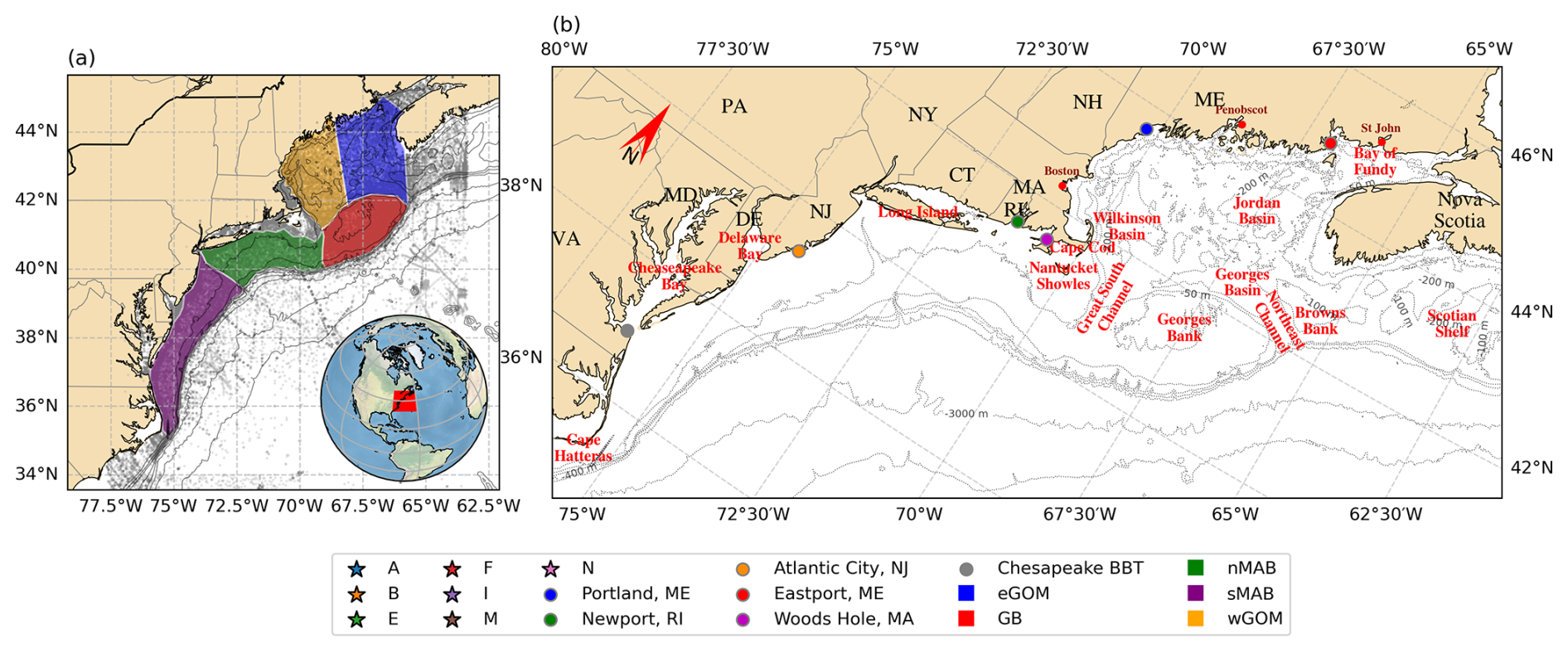
Figure 1 Model domain, Bathymetry, Observations (a), and locations references (b): Stars represent NERACOOS moorings, circles indicate CO-OPS tide gauges, and gray dots show high-resolution CTD data from the World Ocean Database. Colored shapes mark the locations of eastern Gulf of Maine (eGOM), western Gulf of Maine (wGOM), Georges Bank (GB), northern Mid-Atlantic Bight (nMAB), and southern Mid-Atlantic Bight (sMAB).

In the North Atlantic, the Gulf Stream is a subtropical western boundary current that flows along the U.S Coast before separating from the continental margin offshore of Cape Hatteras in North Carolina. This current redistributes heat and saline water poleward, balancing the equatorward transport away from the western boundaries. Detailed depth-stratified estimates indicate transport above 1000 m of 57.3 Sv at Cape Hatteras increasing to 75.6 Sv in the area southeast of Cape Cod (MA), while transport below 1000 m has estimates of 54.5 and 69.9 Sv, respectively (Heiderich and Todd, 2020). Approximately 1000 km downstream from Cape Hatteras, the Gulf Stream begins to destabilize and meander, with its path envelope widening fivefold (Andres, 2016).

The Gulf Stream position has been related to warming of the Northeastern US continental shelf and has influenced the penetration of Labrador water onto North America’s continental margin. The Gulf Stream acts as a valve controlling Labrador Current intrusion, with the mechanism related to the impingement of the Gulf Stream at the Tail of the Grand Banks that influences the Sea Surface Height (SSH). When the Gulf Stream position is closer to the Tail of the Grand Banks, mean SSH increased by 10.8 cm between 2009–2018, when compared with 1993–2008 (Gonçalves Neto et al., 2021). The westward flow of the Labrador Current into the Slope Sea can contribute significantly to the T–S variability on the Gulf of Maine shelf (Petrie and Drinkwater, 1993) through inflow of slope water in the Northeast Channel. Properties of this intruding slope water at the Northeast Channel are related with the Gulf Stream position and the warm-core rings it sheds (Du et al., 2021, 2022). One hypothesis is that these warm-core rings are able to bring modified Gulf Stream Water, which has lower content of nutrients than the slope waters (Townsend et al., 2023).

The Gulf of Maine is a semi-enclosed shelf sea along the NEUS coast almost fully separated from the Atlantic Ocean by Brown Banks and Georges Banks. It is connected with the North Atlantic via the deeper Northeast Channel with about 230 m depth, and the shallower 70 m deep Southwest Channel. The Gulf of Maine has a complex topography with average depth of 150 m and with three major basins, the Wilkinson Basin in the west, Jordan Basin south of Maine and west of Nova Scotia, and Georges Basin, which is connected to the Northeast Channel (Brooks, 1992). Different water mass classification exist in the Gulf of Maine, but here we select the following: The Scotian Shelf Water, with characteristic temperature and salinity of 2 °C and 32.0, respectively; the Warm Slope Water (12 °C, 35.4), and the Labrador Slope Water (6 °C, 34.6). While this classification has been used to identify changes in water masses composition in the Gulf of Maine (Townsend et al., 2010, 2023), it is important to note that the properties of these water masses may vary interannually (Mountain, 2012). Inside Gulf of Maine, the intruding subsurface slope water from Northeast Channel to Jordan Basin is warmer in winter than in summer, contrasting with the surface seasonality of surface waters. These slope waters interact with fresher water from Nova Scotia, strengthening near-surface stratification and suppressing deep convection during winter time (Du et al., 2021).

The cyclonic current system in the Gulf of Maine is characterized by seasonal intensification. During this process, waters originating from the Scotian Shelf and continental slope flow approximately parallel to the coastline and bathymetry, while leaving the area by flowing around Cape Cod or through circulation around Georges Bank that connects the Gulf of Maine to the Slope Sea. This circulation spins up from April to June, strengthens from June to December, then spins down from December to February, when erosion of the stratification deepens the cyclonic circulation, which starts to lose energy due to interaction with bottom friction (Xue et al., 2000). Combined model and observation efforts suggest that convective overturning during winter at Wilkinson Basin is relevant in the deepening of the mixed layer. It can deepen the mixed layer to a depth of about 120 m, while wind stress alone in similar conditions mixes it only to about 80 m. In this case, lateral advection may increase local stability, counteracting pure vertical mixing (Mupparapu and Brown, 2002). The cyclonic circulation presents many features, such as the counterclockwise gyres around Jordan and Wilkinson basins, and the cyclonic circulation connecting Georges Basin and the Northeast Channel (Brooks, 1985). Off the Maine coast, the cyclonic circulation consists of two segments: the Eastern Maine Coastal Current (EMCC) originates from outflows near the Bay of Fundy, with subtidal currents ranging from 0.15 to 0.30 m s⁻¹. In spring and summer, it veers offshore around Penobscot Bay, while during the same season, the Western Maine Coastal Current (WMCC) extends from Penobscot Bay into Massachusetts Bay. EMCC’s currents range between 0.05 to 0.15 m s⁻¹, even though they can leak into the WMCC near Penobscot Bay (ME). Also, during winter, the deep EMCC may decouple from the surface and veer offshore into the cyclonic circulation over Jordan basin (Pettigrew et al., 2005). The WMCC has a strong seasonal signal associated with freshwater inputs in the western Gulf of Maine, although its dynamics is predominantly barotropic (Geyer et al., 2004). During fall and winter, currents are generally weaker and the EMCC has a more continuous flow into the WMCC at the surface. The connectivity peaks twice over the year, first more strongly in winter and then in late spring/early summer (Li et al., 2022).

The Gulf of Maine is influenced by tides, with nearly resonant semi-diurnal tidal responses, a large semidiurnal M₂ tidal current, and tidal range of over 8 m in the Bay of Fundy (Garrett, 1972). In Georges Bank, M₂ tides are relevant to its mean clockwise circulation through tidal rectification (Loder, 1980) and keep the well-mixed waters at areas shallower than 60 m throughout the year (Townsend and Pettigrew, 1996). Over the New England Shelf, a zone of minimum sea level occurs due to encountering tidal waves coming from east of Cape Cod and south of Nantucket Island, a transition region between the tidal environments of the less energetic Mid-Atlantic Bight (MAB) and tidally amplified Gulf of Maine (Chen et al., 2011; He and Wilkin, 2006). Two relevant regions with internal tidal energy flux in the Gulf of Maine are the northeastern flank of Georges Bank, and the Northeast channel, where internal tide M₂ flux has been identified as 0.15, and 1.06 GW, respectively (Chen et al., 2011). Tides have been related to strengthening of the summer circulation in the Gulf of Maine around Georges Bank, Browns Bank by enhancing the coastal current through tidal rectification and mixing (Xue et al., 2000).

Primary productivity in the Gulf of Maine is supported by nitrogen fluxes from multiple sources, including slope waters, rivers, atmospheric deposition, and water column nitrification (Townsend, 1998). Surface chlorophyll concentrations exhibit distinct spatial and temporal patterns, with consistently higher values maintained throughout the year over shallow banks and nearshore, while the lowest concentrations occur in deeper basins and along the shelf-break (Thomas et al., 2003). The region follows the seasonal cycle, with low winter concentrations (< 1 mg m⁻³), an annual maximum during the spring bloom (> 2 mg m⁻³), reduced summer concentrations when vertical stratification is maximal, and a secondary fall bloom beginning in September-November (O'Reilly and Zetlin, 1998; Thomas et al., 2003). During summer stratification, a subsurface chlorophyll maxima develop with concentrations reaching 50 % to 75 % of spring bloom levels (O'Reilly and Zetlin, 1998).

MAB waters are commonly divided into two water masses: shelf water and slope water, which are bounded by the shelfbreak front (Linder and Gawarkiewicz, 1998). The shelf water in MAB is the result of mixing of waters in the Gulf of Maine associated with low salinity water from the Scotian Shelf and the Slope Water that enters the Gulf of Maine through the Northeast Channel (Mountain, 2003, 2012). Oxygen-isotope tracers revealed a connection between shelf water in the Mid-Atlantic Bight and waters originating along the southern shelf of Greenland (Chapman and Beardsley, 1989), with this circulation being driven primarily by the wind stress and secondarily by buoyancy fluxes (Chen and Yang, 2024). At MAB, the equatorward advection associated with surface heat and freshwater exchanges and mixing with saltier slope waters modify the properties of the shelf water (Lentz, 2010). On the surface, interannual variability of salinity is driven largely by river discharge and precipitation (Manning, 1991), with large interannual variations being advected into MAB from the Gulf of Maine (Mountain, 2003). The shelf water in MAB exhibits a cold (< 10 °C) near-bottom water mass that persists over the mid-shelf and outer shelf, from spring to fall. It is a winter remnant feature located between the seasonal thermocline and warmer slope water, with gradual warming from spring to summer at a rate of about 1 °C per month (Lentz, 2017).

In MAB’s tidal currents, the M₂ constituent is the dominant signal representing on average 51.63 % of the total tide signal, with maximum of 10 cm s⁻¹ on the mid-shelf, local maxima near the mouths of estuaries, and a phase that sweeps from north to south. Seasonal stratification and internal waves are associated with localized seasonal and interannual tidal amplitude variations in Nantucket Shoals (Brunner and Lwiza, 2020). Internal waves have been found to be influenced by the Gulf Stream and the shelfbreak front. The shelfbreak front can decrease by about 10 % the generation of topographic internal tides, while the Gulf Stream can prevent internal tides from radiating into the North Atlantic depending on the angle of incidence (Kelly and Lermusiaux, 2016).

Chlorophyll concentration in Mid-Atlantic Bight has two major periods of enhanced activity over the year, corresponding to fall-winter and spring periods (Xu et al., 2011). Nearshore areas close to estuaries are regions where chlorophyll is high throughout the year, similarly to the Gulf of Maine (O'Reilly and Zetlin, 1998), with outflow plumes of Chesapeake and Delaware Bay areas having higher annual rates of net primary productivity than the mid-shelf area to the north of Chesapeake and areas influenced by the Gulf Stream (Filippino et al., 2011). Seasonal vertical stratification has an important role in the vertical mixing on the continental shelf and on the control of nitrogen availability, with the near shelf front transiting from well mixed during the winter to stratified in summer (Lentz, 2003; Rasmussen et al., 2005).

3 Methods

3.1 Model Configuration

The results in this work were produced by coupling the Geophysical Fluid Dynamics Laboratory’s (GFDL) MOM6 and COBALT biogeochemical model (Adcroft et al., 2019; Stock et al., 2014, 2020). The configurations of MOM6 and COBALT largely followed configurations and datasets (initial conditions, boundary conditions and surface forcing) used in Ross et al. (2023) (R23, hereinafter). This hindcast simulation represents the period from 1993 to 2019. The datasets and differences in parameterization choices from R23 and other model configurations are briefly described below.

The model employs a z^* coordinate with 75 layers following R23 with near-surface layer thickness of 2 m that increases progressively to a maximum of 250 m at 6500 m. The time steps are defined as 600 s for the baroclinic component, 1800 s for coupling, thermodynamics, and biogeochemistry, while the time-varying barotropic time step is constrained to 90 % of the CFL-limited maximum stable step. A Flather (1976) radiation boundary condition was used for barotropic velocity and subtidal, and tidal sea level, while the baroclinic flow was configured using Orlanski (1976) radiation scheme and nudging following (Marchesiello et al., 2001) from The Copernicus Marine Global Ocean Reanalysis (GLORYS). Lateral boundary conditions nudging had time scales of 5 d for inflow and 360 for outflow considering the baroclinic component. Lateral boundaries were associated with nudging close to the borders of the domain in order to constrain the separation of the Gulf Stream at Cape Hatteras. This is a strategy similar to the one adopted by Azevedo Correia De Souza et al. (2023). A maximum damping rate of 7 d is applied at the borders for temperature and salinity, reaching timescales of several thousand days in the domain center to minimize interior constraints.

The topography was linearly interpolated from the General Bathymetric Chart of the Oceans (GEBCO) (GEBCO Bathymetric Compilation Group 2023, 2023) and didn’t require smoothing. A horizontal Arakawa C grid with 430 × 396 tracer points and a nominal resolution of approximately $\mathrm{1}/\mathrm{25}$° is interpolated from a subset of a $\mathrm{1}/\mathrm{12}$° grid of the North Atlantic (Chassignet and Xu, 2017), with typical zonal and meridional distances between grid points of approximately 4 km at mid-latitudes. The grid is defined from South Carolina to Nova Scotia and includes the Mid-Atlantic Bight, Gulf of Maine, and Bay of Fundy (Fig. 1).

Starting from R23, a calibration phase testing several combinations of parameterizations and parameters determined the final model configuration. The tests combined vertical mixing schemes including KPP (Large et al., 1994), ePBL (Hallberg, 2013), shear stress parameterization (Jackson et al., 2008), mixed-layer eddy parameterization (Fox-Kemper et al., 2008; Fox-Kemper and Ferrari, 2008) and different advection-Coriolis schemes (Arakawa and Lamb, 1981; Sadourny, 1975). Table 1 summarizes the main configurations of MOM6-COBALT-NEUS25. The Arakawa and Lamb (1981) coriolis-advective scheme better confined tracer fields to continental shelf bathymetry than Sadourny (1975) scheme (not shown). Sadourny (1975) energy-conserving scheme tends to spuriously accumulate enstrophy at smaller scales which could be problematic for high resolution models. When coupled with the horizontal viscosity scheme (maximum between biharmonic and Smagorinsky) under the R23 configuration, Arakawa and Lamb (1981) advective scheme rapidly eroded the ocean mesoscale structure. In this context, increasing the Smagorinsky viscosity corrected the erosion, perhaps by better constraining horizontal viscosity relative to vertical viscosity, which affected the inverse energy cascade, though the exact mechanism remains unclear. The model employs a hybrid boundary layer mixing scheme based on the maximum between ePBL and KPP diffusivities. R23 mentioned improved description of bottom temperature when employing the mixed-layer parameterization (Fox-Kemper et al., 2008), however this was not found in our calibration phase.

Adcroft and Campin (2004)Large et al. (1994); Reichl and Hallberg (2018)Jackson et al. (2008)Griffies et al. (2000)Adcroft et al. (2019)Flather (1976)Marchesiello et al. (2001); Orlanski (1976)Arakawa and Lamb (1981)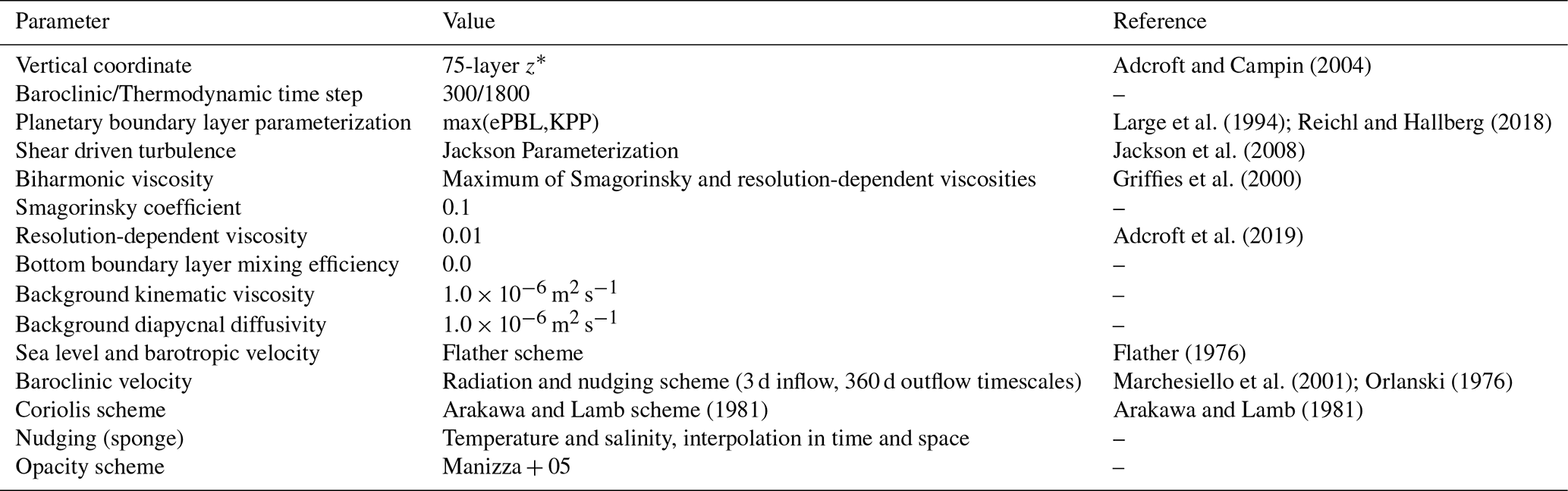

Table 1 Model Parameters

A summary of the datasets and respective variables used to produce the initial conditions, boundary conditions and surface forcing fields for MOM6 and COBALT are presented in Table A1. MOM6 was initialized directly from interpolated initial conditions from GLORYS in 1993 following R23, and COBALT initialized from the interpolated information from a global MOM6 + COBALT simulation (Stock et al., 2014), World Ocean Atlas (Garcia et al., 2024b, a), and a fit using ESPER (Carter et al., 2021). Riverine forcing is also present in the coupled model. Since our domain of NEUS25 is relatively restricted and is continuously forced by boundary conditions, the spin-up requires less than one month to start presenting reliable information at $\mathrm{1}/\mathrm{25}$th resolution.

The Copernicus Marine Global Ocean Reanalysis (GLORYS) provides eddy-resolving ($\mathrm{1}/\mathrm{12}$°) global simulation results from 1993 onward, assimilating observational data (Jean-Michel et al., 2021). The assimilated data consist of 0.25° AVHRR sea surface temperature, altimeter information, in situ temperature and salinity profiles, and sea ice extent over polar oceans (Drévillon et al., 2025). ERA5 is a fifth-generation ECMWF reanalysis of global weather and climate, representing a detailed atmospheric record beginning in 1940. It combines model results with global observations through data assimilation performed every 12 h (Hersbach et al., 2020). TPXO9 is a global ocean tidal model for barotropic tides that optimally fits the Laplace tidal equations using bathymetry and satellite altimeter data. It provides gridded harmonic constants for semidiurnal (M₂, S₂, N₂, K₂), diurnal (K₁, O₁, P₁, Q₁), two long-period (Mf, MM), and three nonlinear (M₄, MS₄, MN₄) tidal constituents. The specific constituents adopted in MOM6 are listed in Table A1. River discharge data are obtained from the Global Flood Awareness System (GloFAS), an operational forecasting and monitoring system developed by the European Commission's Copernicus Emergency Management Service. This satellite-based service utilizes Copernicus Sentinel-1 Synthetic Aperture Radar (SAR) data at 0.1° resolution (Harrigan et al., 2021).

The World Ocean Atlas 23 (Garcia et al., 2024b, a) consists of objectively analyzed, quality controlled fields based on the World Ocean Database, that can be used in creating boundary and/or initial conditions for ocean models. The ESPER multiple regression algorithm (Carter et al., 2021) is used to fit the Alkalinity and DIC based on salinity and potential temperature in the boundary conditions from WOA23 considering the monthly climatology product, without the year-varying adjustment applied by R23. The implications are discussed in Sect. 5. We used the climatology of Stock et al. (2014) to determine multiple variables required by COBALT in both initial and boundary conditions. This is a global ocean-ice-ecosystem model that was able to capture cross-biome features and observation-based planktonic web fluxes estimates. The River Chemistry for the U.S. Coast (RC4USCoast) is a historical dataset containing river chemistry and discharge for 140 monitoring sites of the US Coast, from 1950 to 2022, derived from the Water Quality Database of the US Geological Survey (USGS), and including river discharge from the U.S. Army Corps of Engineers and the USGS’s Surface-Water Monthly Statistics for the Nation (Gomez et al., 2022, 2023). For the atmosphere, historical atmospheric CO₂ concentrations up to 2014 and its extension under the SSP2-4.5 are used (Meinshausen et al., 2020). Monthly climatologies of GFDL’s ESM4.1 earth system model (Dunne et al., 2020) provided the wet and dry deposition of NO₃ and NH₄, and lithogenic dust. Iron was assumed to represent 3.5 % of the dust, while dry deposition of phosphorus assumed a concentration of 563 ppm, where 22 % is available for biology (Baker and Croot, 2010; Herbert et al., 2018) . These approaches followed (Stock et al., 2020) and R23.

Our model initialization starts directly from GLORYS temperature and salinity field in a similar manner to R23. Given the relatively restricted and shallow domain we are working, the biogeochemistry in the domain spin-up takes about 3 months to adjust from the climatological conditions, which is associated with the relatively shallow environment on the continental shelf and the intense horizontal and vertical mixing associated with the presence of the Gulf Stream on the slope. We include the spin-up period of the model in the model evaluation since it is relatively short.

3.2 Observations

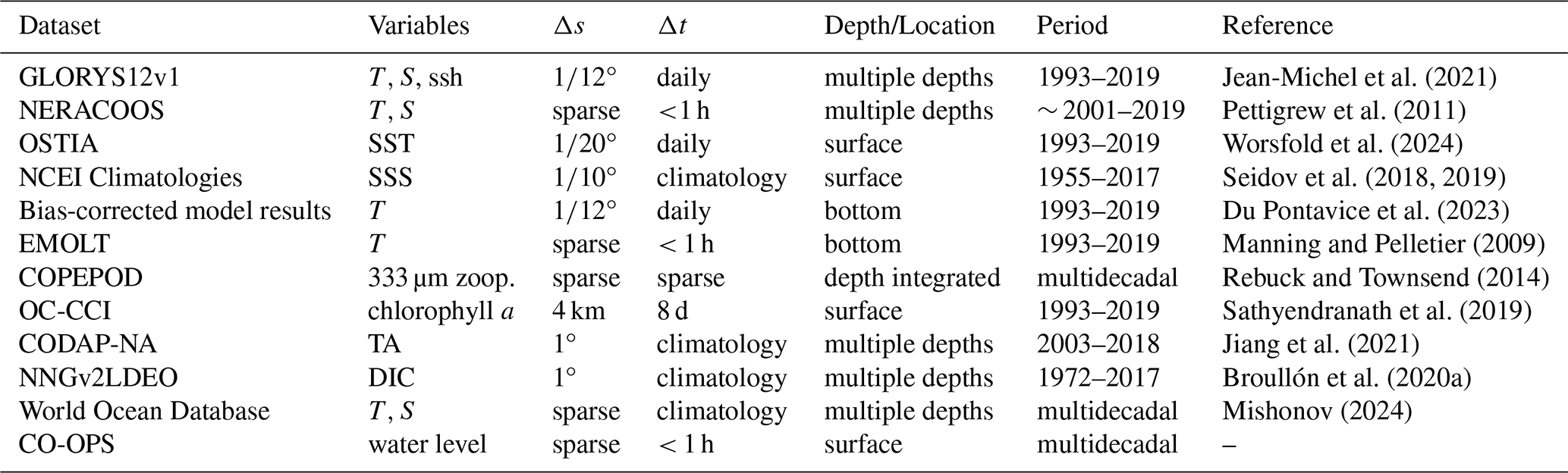
MOM6-COBALT-NEUS25 results were evaluated by comparing simulated fields against in-situ observations, satellite-derived products, and climatological datasets. Our strategy targeted physical oceanographic variables (temperature, salinity, sea level), and biogeochemical parameters (chlorophyll, NO₃, zooplankton biomass). The data products used to evaluate the coupled model results are summarized in Table 2. In our evaluation, delta difference maps are used for comparisons between data references and MOM6-COBALT-NEUS25 results. Their color palettes are configured to be comparable with R23 whenever possible. We present a brief overview of the datasets below.

Jean-Michel et al. (2021)Pettigrew et al. (2011)Worsfold et al. (2024)Seidov et al. (2018, 2019)Du Pontavice et al. (2023)Manning and Pelletier (2009)Rebuck and Townsend (2014)Sathyendranath et al. (2019)Jiang et al. (2021)Broullón et al. (2020a)Mishonov (2024)

Table 2 Data products used to evaluate the coupled model. Spatial and temporal resolution are represented, respectively by Δ s and Δt.

The Northeastern Regional Association of Coastal Ocean Observing Systems (NERACOOS) has deployed oceanographic moorings in the Gulf of Maine since 2001. These buoys provide high-temporal resolution measurements enabling detailed assessment of tracer field variability. Temperature, salinity, and Acoustic Doppler Current Profiler (ADCP) sensors record information at various depths in the water column, with the data being maintained and made available on the NERACOOS website (neracoos.org). The positions of the buoys are shown in Fig. 1.

Sea surface temperature (SST) is evaluated using a long-term, reprocessed dataset SST (OSTIA) (Worsfold et al., 2024) with a grid resolution of 0.05°. This dataset is a daily gap-free analysis that uses in-situ and satellite data processed at Met Office (UK). Daily sea level gridded data based on satellite observations from 1993 to the present were produced by Copernicus Climate Change Service (C3S sea level dataset) (Lopez, 2018).

Sea surface salinity evaluation is based on the National Centers for Environmental Information (NCEI) Northwest Atlantic Regional Climatology (Seidov et al., 2018, 2019), which is derived from World Ocean Database and presents a resolution of 0.1°. Despite the existence of satellite data products for salinity, their relatively short time range precludes the assessment at longer timescales and makes it more advantageous to use the regional climatology for evaluation.

Simulated bottom temperature in the northeast U.S. continental shelf from MOM6-COBALT-NEUS25 was evaluated using two distinct datasets. The first consists of a high-resolution long-term bottom temperature product, created based on a bias-corrected ROMS simulation, and two global ocean reanalysis (GLORYS12v1 and PSY4V31) (Du Pontavice et al., 2023), with good performance in reproducing both seasonal and annual variability of reference datasets. It enables the evaluation of the seasonal horizontal distribution of bottom temperature on the continental shelf. The second dataset consists of temperature time series measured by thermistors in lobster traps (Manning and Pelletier, 2009) distributed along the western edge of the Gulf of Maine and along the shelf edge in the northern Mid-Atlantic Bight in water depths ranging from 1–300 m. It complements the spatial analysis by including detailed temporal variability at multiple locations.

World Ocean Database is a quality-controlled dataset including more than 18.6 million oceanographic casts consisting of up to 3.13 billion individual profile measurements. Here we select only high-resolution CTD information with temperature and salinity information (Mishonov, 2024) to evaluate the seasonal vertical structure of temperature and salinity along the continental shelf based on the subregions defined in Fig. 1.

Long-term measurements of sea level using tide gauges operated and maintained by CO-OPS (2018) are used in the validation of the sea surface elevation at the coast .

The following datasets present biogeochemistry data in terms of nutrients, chlorophyll, and zooplankton, useful in the evaluation of seasonal results. A data collection ranging from 1932 to 2011 was organized by Rebuck and Townsend (2014) in the Gulf of Maine including dissolved inorganic nitrogen, silicate and phosphate from several sources, such as the World Ocean Database, and Integrated Science Data management among others. These data are used to calculate seasonal climatologies of NO₃ + NO₂ and PO₄. Chlorophyll was obtained from the Ocean-Colour Climate Change Initiative (OC-CCI), which derives chlorophyll a from ocean-colour data. It uses the Medium Spectral Resolution Imaging Spectrometer (MERIS) from the European Space Agency, the Sea-viewing Wide-Field-of-view Sensor (SeaWiFS), and Moderate-resolution Imaging Spectroradiometer-Aqua (MODIS-Aqua) from National Oceanic and Atmospheric Administration, with a time series covering the period from late 1997 to end of 2018 at 4 km resolution (Sathyendranath et al., 2019), which closely matches the model’s resolution. The Coastal & Oceanic Plankton Ecology, Production & Observation Database (COPEPOD) is a global online database that consolidates 60 years of plankton monitoring. It has been created by the National Marine Fisheries Service with data from several fisheries and research institutes around the world (Moriarty and O'Brien, 2013). This dataset provides the monthly 200 m average biomass estimate of epipelagic mesozooplankton and is compared with the mesozooplankton simulated by MOM6-COBALT-NEUS25.

Carbon chemistry is evaluated through total dissolved inorganic carbon (DIC) and total alkalinity (TA). NNGv2LDEO (Table 2) consists of a feedforward neural network calibrated with the Lamont-Doherty Earth Observatory datasets (Takahashi et al., 2017), Global Ocean Data Analysis Project version 2.2019 (Olsen et al., 2019), among others. The DIC climatology was produced by passing WOA23 temperature, salinity, and oxygen climatologies – along with phosphate, nitrate, and silicate fields derived from those same variables using a different neural network (Bittig et al., 2018) – through the trained NNGv2LDEO network (Broullón et al., 2020a). NNGv2LDEO climatology will be referred hereinafter as “Broullón climatology”. The Coastal Ocean Data Analysis Product in North America (CODAP-NA) (Jiang et al., 2022); is a data product focused on coastal ocean acidification, with two decades of discrete measurements of several carbon system parameters, nutrients and oxygen from the North American continental shelves including TA.

4 Results

4.1 Circulation

Average SSH results of MOM6-COBALT-NEUS25 generally represent the separation of the Gulf Stream at Cape Hatteras, but exhibits a northward bias west of 67.5° W of approximately 0.5° that makes it closer to the shelf, relative to both GLORYS SSH and CMEMS satellite ADT L4 product (Fig. 2) in the period from 1993 to 2019. Following separation from the continental slope off Cape Hatteras, MOM6's Gulf Stream displays a tendency to meander northward along the Mid-Atlantic Bight shelfbreak, contrasting with the more southerly path demonstrated in both the CMEMS satellite SSH L4 product and GLORYS reanalysis. Monthly averages of all three datasets reveal paths of Gulf Stream with pronounced presence of meanders in CMEMS reaching the shelf break south of the Scotian Shelf. These processes, associated with mesoscale activity and warm-core rings, have significant influence on slope water intrusions into the Gulf of Maine (Du et al., 2022). Even though the reduced meandering in MOM6 and GLORYS could lead to misrepresentation of tracer fields in the Gulf of Maine and biases in the primary production simulation by COBALT, the model and reanalysis are able to realistically simulate the waters in the Gulf of Maine. Bias-correction of lateral boundary nudging and initial conditions can potentially improve the solution, but they often return mixed results with no clear advantage over using original reanalysis outputs (e.g López et al., 2020; Lehmann et al., 2009).

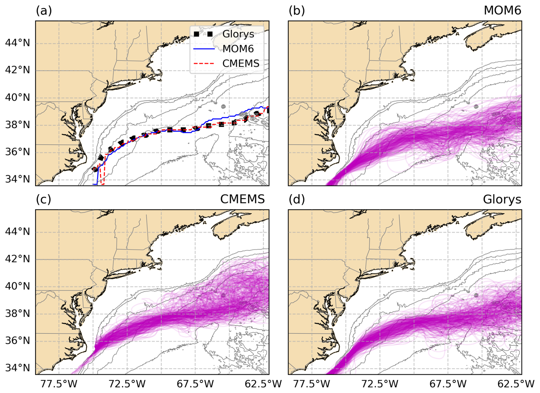
Figure 2 Path comparison of the Gulf Stream for the period between the years of 1993–1994 across MOM6, CMEMS satellite SSH L4 product and GLORYS. Position of the Gulf Stream based on the maximum standard deviation of SSH (a). In the remaining panels (b–d), magenta lines represent the 0 m contour of monthly SSH anomaly. Gray lines represent isobaths of 1000, 2000, 3000, 4000, and 5000 m

Seasonal averages of MOM6-COBALT-NEUS25, GLORYS and their comparison are shown in Fig. 3. On the slope, the average position of the Gulf Stream is represented by the largest horizontal SSH gradients. Our simulation represents the region on the Slope Sea marked by lower SSH values (< −0.55 m) and the areas south of the Gulf Stream's North Wall where the highest SSH values are present. On the continental shelf, MOM6-COBALT-NEUS25 has isolines of SSH (−0.5 m) pattern that are more complex than GLORYS', marking features associated with the Northeastern Channel in the Gulf of Maine and the region influenced by Georges Bank. On the slope domain, the model underestimates positive SSH values, and overestimates negative SSH values (Fig. 3i to l).

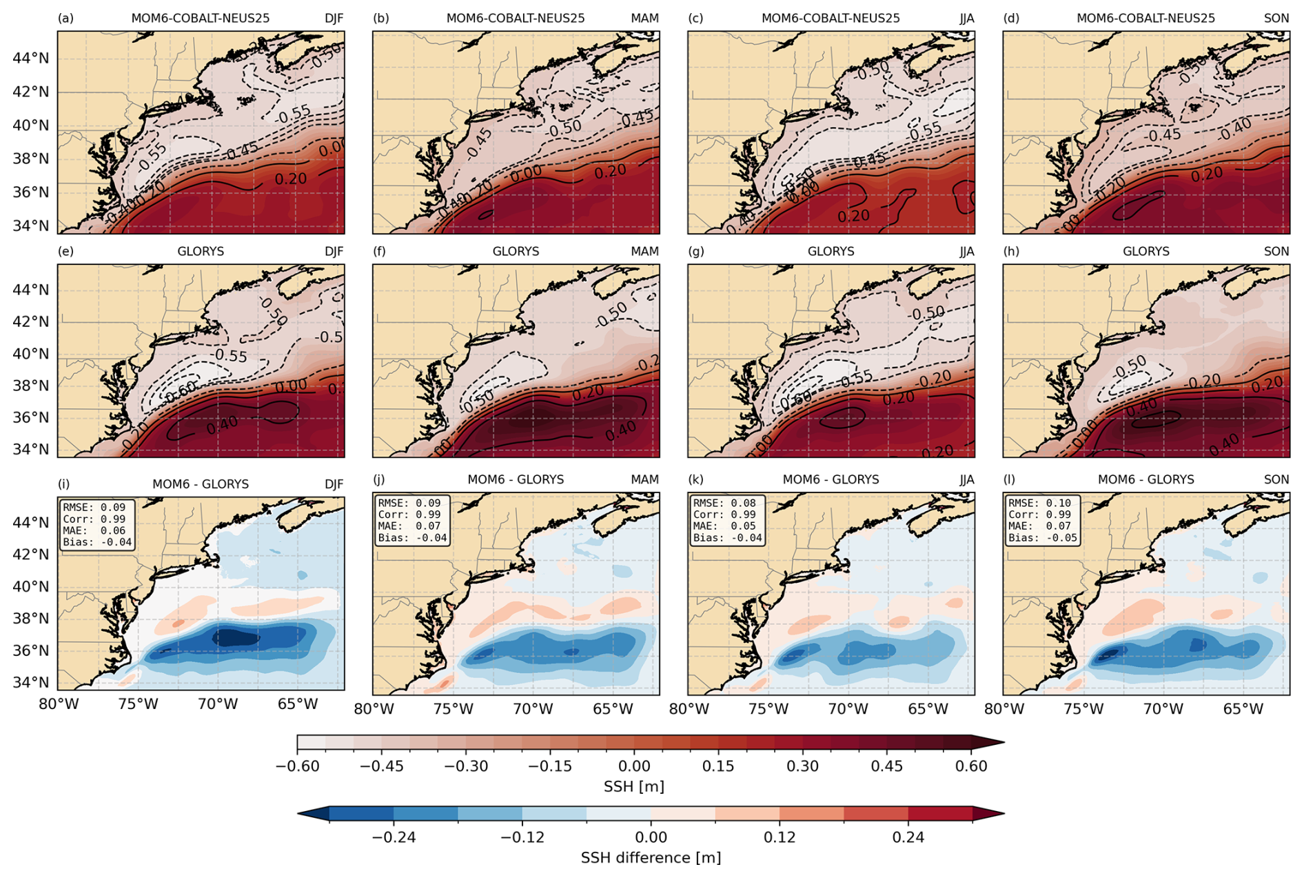
Figure 3 Seasonal averages of SSH considering MOM6-COBALT-NEUS25 (a–d), GLORYS (e–h) and their difference, MOM6-COBALT-NEUS25 – GLORYS (i–l). Black contours and filled contours represent SSH intervals.

Currents at the surface and at 75 m show the general structure in the Gulf of Maine described in Sect. 1 is reproduced, with the representation of features such as the Shelf Break Jet, WMCC, EMCC, the anticyclonic circulation around Georges Banks, and the cyclonic circulation connecting Georges Basin with the Northeast Channel (Fig. 4). The intensification of the cyclonic circulation in the Gulf of Maine associated with seasonal surface heat flux (Xue et al., 2000) occurs in the model, with stronger circulation parallel to the coast line, with a WMCC flowing parallel to NH coast, differently from winter. The analysis reinforces the relevance of topography to the circulation in the Gulf of Maine, with the currents generally following isobaths, as expected at first order from the tendency of the flow to follow the Taylor-Proudman theorem and vorticity constraints. The cyclonic recirculation in Georges, Wilkinson and Jordan Basin occupies the entire water column in all seasons (not shown). The slope waters pathways into the Gulf of Maine are defined by the intensified flow (> 0.16 m s⁻¹) at the northern wall of the Northeastern Channel, with part of flow being redirected into the recirculation in Georges Basin and Browns Bank, part of being redirected into the interior of the Gulf of Maine, and part flowing parallel to the coastline.

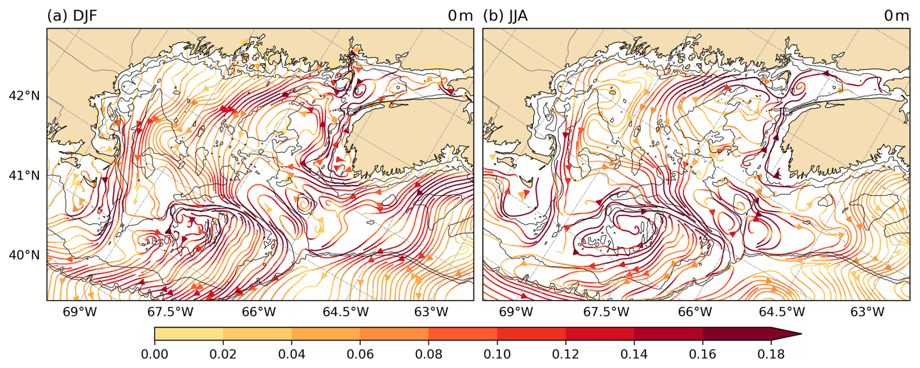
Figure 4 Winter (a) and summer (b) integral curves of the instantaneous MOM6 surface velocity field, computed via numerical integration of the tangent vector field.

Hovmöller Diagrams of daily composites for the period between 2009 and 2019 of NERACOOS ADCP moorings show the model reproduces the seasonal structure with mixed performance, based on a bulk correlation displayed in Fig. 5 for moorings A, I, M, N (Fig. 1). For along-bathymetric currents, larger error metrics (RMSE, MAE, and bias) are present and are likely a consequence of the higher magnitudes of these currents. At mooring M (Figs. 1, 5M), the low correlations (< 0.1) are associated with the relatively low currents (< 6 cm s⁻¹), where a relatively poor signal-to-noise ratio occurs. In the Gulf of Maine, the grid resolution does not resolve the first Rossby radius of deformation Radius (Hallberg, 2013), which may contribute to the low correlation in the solution of currents at different moorings.

Even though relevant differences in magnitude of the along-bathymetry currents at mooring N (Figs. 1, 5N) occur, some similarities are still observed. Two seasonal regimes are evident in mooring N following the NERACOOS observations. The first occurs in mid-year (approximately days 180–260), while the second occurs during the remainder of the year. The mid-year structure has more intense currents (< 10 cm s⁻¹) at the subsurface, with its core at about 100 m. The second, on the other hand, shows surface intensified currents, while currents flow out of the Gulf of Maine below approximately 70 m. During mid-year, the current structure is roughly reproduced by the model, with a relatively deeper penetration of the current with its core at about 50 m and surface along-bathymetry currents near 0 cm s⁻¹. The current intensification in the model does not reach the bottom, similarly to the observations. During other periods, the surface intensification biases reaches about 8 cm s⁻¹, while at depth the model shows currents that approach 0 cm s⁻¹.

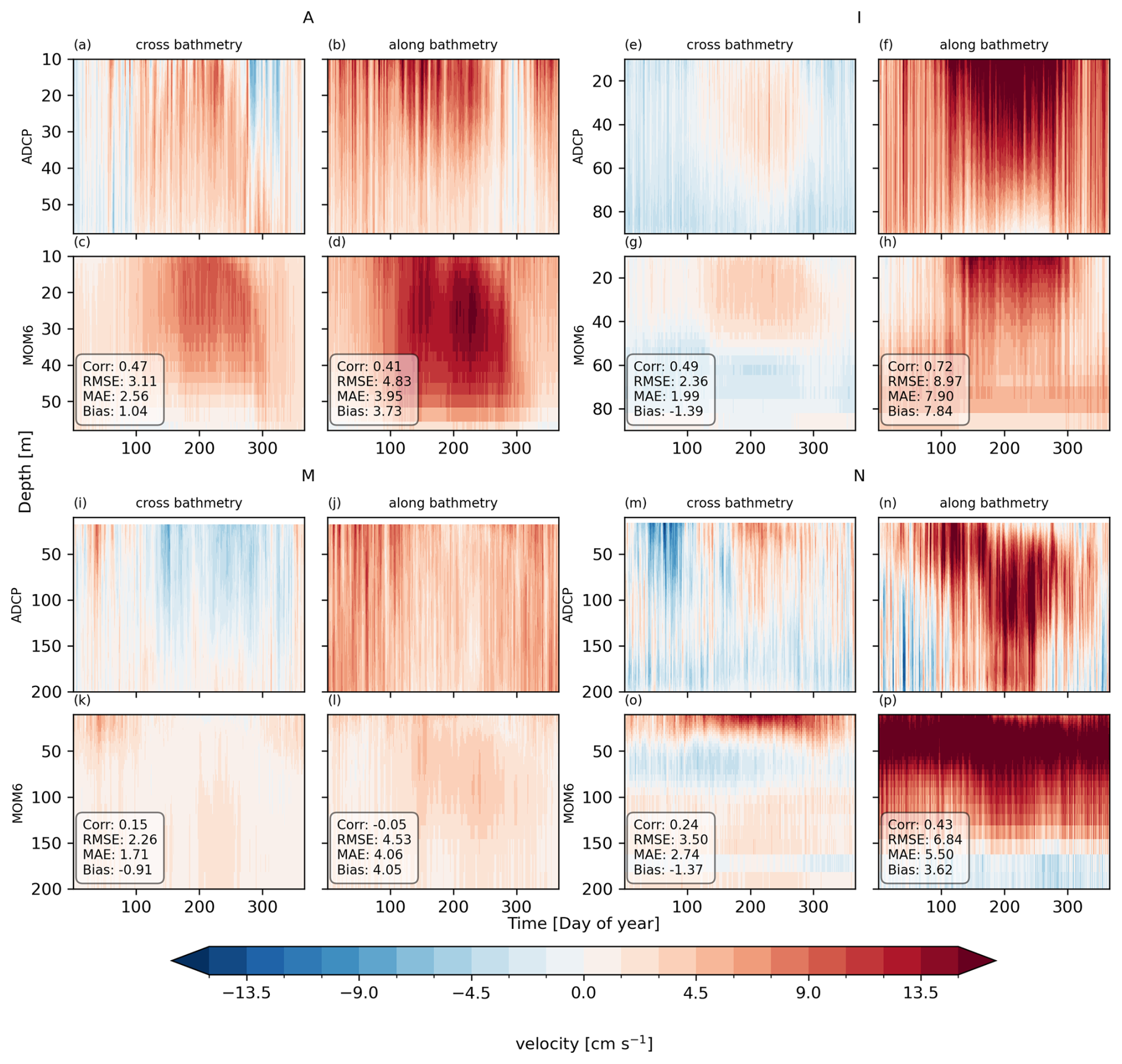
Figure 5 Hovmöller diagram of currents (daily composite) measured by NERACOOS ADCP and simulated by MOM6-COBALT-NEUS25 (row labels), considering cross-, and along-bathymetry currents. Moorings (A, I, M, N) are referenced by the subtitles. Positive values of along-bathymetry panels are referenced as equatorward flow for moorings A, and I, towards the Gulf of Maine at mooring N, and in the cyclonic direction at mooring M. In the cross bathymetric panels, positive values are perpendicular and to the right of the along-bathymetry direction. The evaluation period spans the years between 2009 to 2019 and correlation values represent the correlation between observed and modeled currents computed over all time-depth pairs (flattened time-depth matrix). The position of the moorings is found in Fig. 1

4.2 Temperature and Salinity

4.2.1 Seasonal surface fields

Sea surface temperature (SST) patterns provide further metrics to evaluate the Gulf Stream structure and the continental slope and shelf fields. The SST representation in MOM6-COBALT-NEUS25 is evaluated using OSTIA level 4 data product for the entire period of the simulation. Figure 6 shows a seasonal climatological comparison between the SST of MOM6, OSTIA and their difference. Domain-averaged biases are relatively small (< 0.2 °C) across all seasons, with the surface 20 °C isotherm delimiting warmer waters in the domain of the Gulf Stream and Slope Sea, and cooler waters on the continental shelf. A similar GLORYS evaluation provides additional context for performance assessment (Fig. A1). In general, MOM6 shows some similar statistics compared with GLORYS, with absolute biases being generally less than 0.19 °C in MOM6 compared to 0.25 °C in GLORYS on average. Similarly, MOM6 shows similar mean absolute error (MAE) values (0.40 °C). Spatial correlation also present similar values (0.99 to 1.0), while MOM6 has a slight higher RMSE (0.63 °C) than GLORYS (0.55 °C).

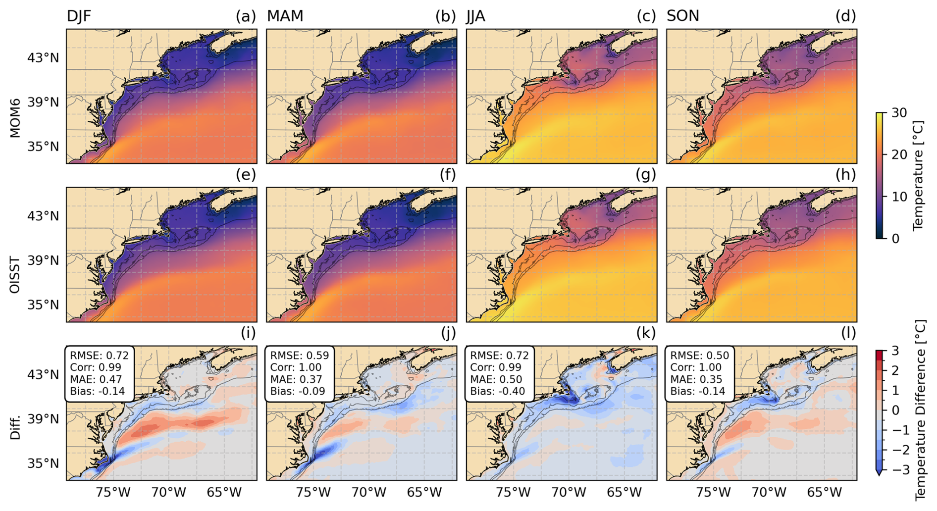
Figure 6 Seasonal averages of sea surface temperature considering MOM6 (a–d), OSTIA SST (e–h) and their differences (i–l, MOM6 – OSTIA). OSTIA SST was interpolated (bilinear) into MOM6 horizontal grid. Black contours are the isobaths of 40, 80, and 400 m.

MOM6-COBALT-NEUS25 representation of the Gulf Stream separation in Cape Hatteras (Figs. 6, 2), leads to an improved description of the SST in the Slope Sea and in the Gulf Stream domains relative to NWA12 (Ross et al., 2023, Fig. 3). Considering the Gulf Stream and Slope Sea regions, DJF and SON have the warmest positive bias typically ranging between +0.5 and +1.5 °C, followed by MAM and JJA when biases are typically between 0.0 and 1.0 °C (Fig. 6). The higher biases in Winter and Fall in MOM6 represent remnants of the Gulf Stream meandering northward of its most typical position after the separation from Cape Hatteras.

In the Gulf of Maine, the seasonal differences between MOM6-COBALT-NEUS25 SST and OSTIA are typically below 0.5 °C – these values are comparable with a similar evaluation of the mean SST using eight reanalysis products (Castillo-Trujillo et al., 2023). During JJA and SON, MOM6-COBALT-NEUS25 shows biases up to −1 °C in the Nova Scotia and a patch of strong negative biases (< −2 °C) south of Cape Cod, which is also identifiable in R23 evaluation. These seasonal representations are an improvement relative to GLORYS (Fig. A1) in the coast of Maine, Nova Scotia, and Georges Bank when considering JJA and SON. At these regions GLORYS presents local differences that are larger than 3 °C likely due to absence of tides representation in the reanalysis.

The seasonal sea surface salinity (SSS) represented by MOM6 is generally similar to NCEI regional climatology (Fig. 7) considering the period from 1993 to 2019, with domain-averaged absolute bias presenting values typically lower than 0.1, and spatial correlation higher than 0.95. The isohaline of 34 roughly marks the limit between the continental shelf and the continental slope, with NCEI climatology showing slight deviations from this pattern in the region of the Mid-Atlantic Bight. The lowest salinities (< 30) occur along the coast in the NCEI climatology, with emphasis on the Scotian Shelf and during the spring (MAM), and summer (JJA), when a fresher strip of water between the coast of Maine and Cape Hatteras is present. In MOM6, this fresher water feature is not represented, appearing as a positive bias, with salinity values up to +1.8 saltier during spring (Fig. 7c, k). Along Chesapeake and Delaware bays, MOM6 shows fresher salinity biases that, throughout the year, may exceed −2.0, and continues as a fresh bias tongue over the shelfbreak in DJF, JJA, and SON with values varying approximately between −0.4, and −1.2. In the Gulf of Maine, Georges Bank and areas beyond the 400 m isobath show more moderate salinity biases between ±0.4. In general, MOM6-COBALT-NEUS25 biases on the shelf and slope in the domain between Cape Hatteras and the Scotian Shelf are lower than those in R23, where positive biases (roughly between +0.4 and +1.2) were present. Compared to GLORYS, MOM6-COBALT-NEUS25 exhibits similar spatial correlation and bias magnitudes, but slightly elevated RMSE values during spring and summer seasons (Figs. 7, A2). MOM6-COBALT-NEUS25 exhibits a salinity drift pattern similar to that of GLORYS (Fig. A3). The absolute salinity difference between MOM6-COBALT-NEUS25 and GLORYS are generally lower than 0.2 in the period between 1993 and 2019 and shows no significant trend over time indicating an evaporative-freshwater flux balance.

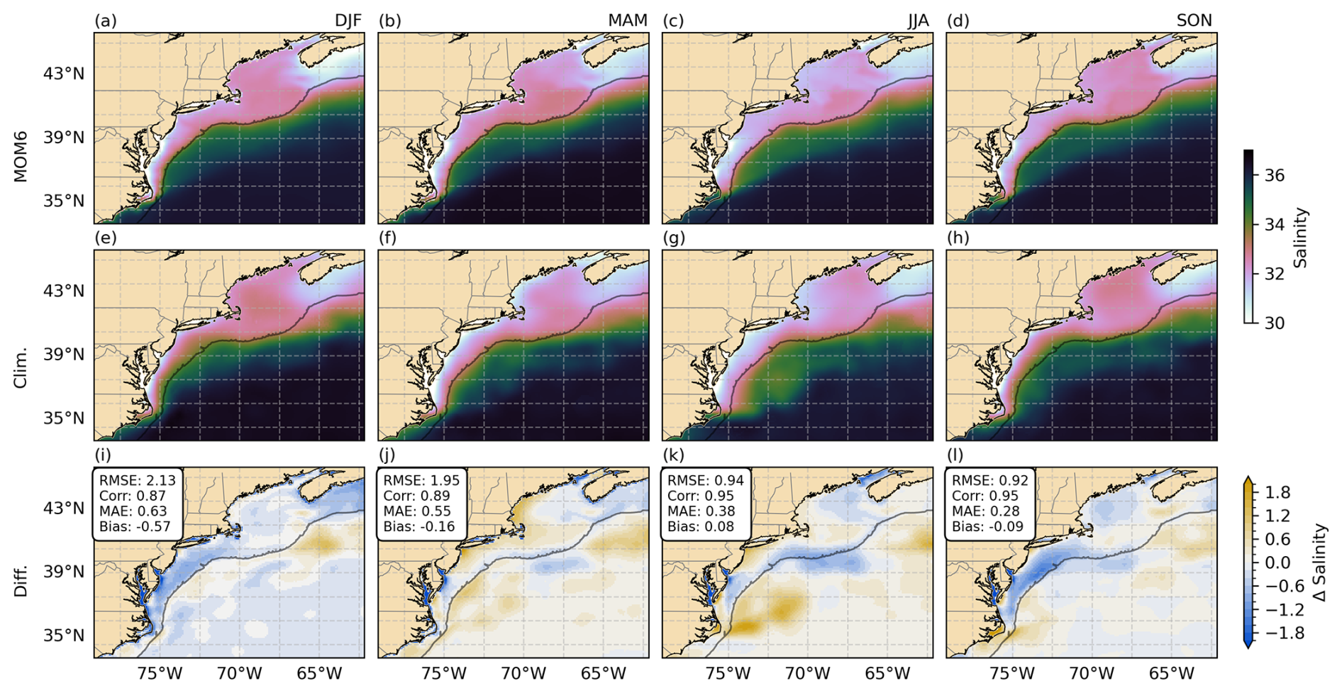
Figure 7 Seasonal averages of sea surface salinity from MOM6 (a–d) and NCEI regional climatologies (Clim., e–h) and seasonal differences (MOM6 – Clim., i–l). Black contour indicates the 400 m isobath, roughly representing the position of the shelf break. MOM6 results were upscaled to NCEI climatologies resolution (0.1°) by binning corresponding areas and calculating averages.

4.2.2 Bottom temperature evaluation

Seasonal fields of bottom temperature of MOM6 are comparable to the seasonal averages dataset of Du Pontavice et al. (2023) having absolute averaged-domain biases lower than 1 °C, and spatial correlation higher than 0.77 (Fig. 8). In the Mid-Atlantic Bight, the seasonal maximum migrates spatially throughout the year: during winter and spring (Fig. 8a, b, e, f), maximum temperature occurs at the mid-shelf and shelf break (> 40 m), while in summer and fall (Fig. 8c, d, g, h), they shift to the inner-shelf (< 40 m). The Gulf of Maine has a similar seasonal pattern, with higher temperatures (> 10 °C) associated with locations closer to the coast during summer and fall, whereas near-coastal waters have typically lower temperatures (< 8 °C) in winter and spring.

Model performance varies seasonally, with MOM6 bottom temperature showing its best performance during fall across all subdomains in terms of spatial correlation (0.94). A warm bias varying from 0.0 to 2.0 °C is present in waters shallower than 80 m during spring and summer along the continental shelf of Mid-Atlantic Bight and Georges Banks, which is potentially linked with the overmixing associated with the upper ocean boundary layer scheme (section Methods) and could lead to enhanced mixing between warmer surface waters and colder bottom waters. On the other hand, the model shows cold biases (< 2 °C) near the shelf break throughout the year relative to Du Pontavice et al. (2023). In the Gulf of Maine, areas deeper than 40 m exhibit cold biases usually between 0.0 to 1.0 °C in winter, summer, and fall, while spring shows bias up to −2 °C.

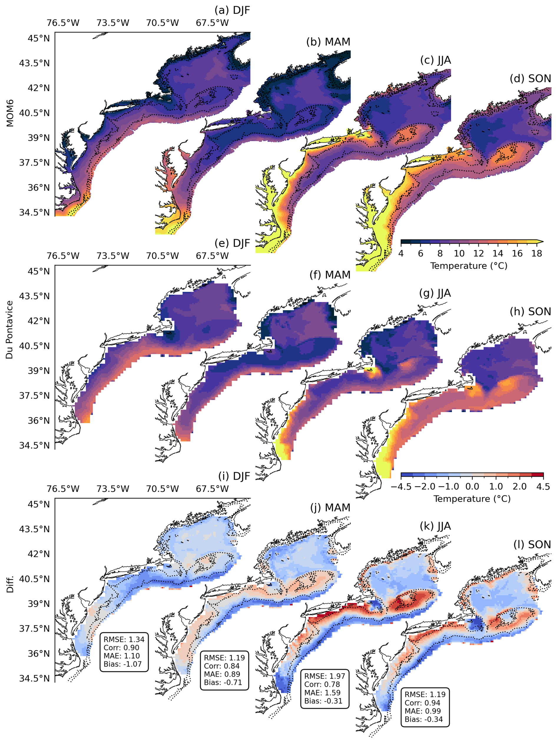
Figure 8 Seasonal averages of bottom temperature in MOM6 (a–d), Du Pontavice bottom temperature dataset (e–h), and their difference (MOM6 – duPontavice, i–l) considering the period between 1993 to 2019. Dotted lines correspond to the isobaths of 40 and 80 m. MOM6 results were upscaled to Du Pontavice’s resolution ($\mathrm{1}/\mathrm{12}$°) by binning corresponding areas and calculating averages.

Bottom temperatures from MOM6-COBALT-NEUS25 are evaluated against eMOLT lobster trap thermistors measurements (1993–2014) along with an analysis of GLORYS results (Figs. 9 and A5). Only datasets containing over one hundred observation days were included in this analysis. MOM6 and GLORYS have similar performance in simulating bottom temperatures time series (Fig. 9), with MOM6 presenting more sites with correlation greater than 0.95 within 0–200 m isobath range. Both model and reanalysis have decreased skill in deep waters (> 200 m) along the shelf break, where correlations drop below 0.85, normalized standard deviations fall below 0.7 °C, and mean bias exceeds 2.0 °C. On the mid- to outer-shelf south of Massachusetts/Rhode Island and close to the 60 m isobath, MOM6 displays a cold bias up to 2–3 °C relative to GLORYS. The spatial statistics maps reveal regional performance variations, with MOM6 achieving higher correlation coefficients, normalized standard deviations closer to unity, and lower absolute mean biases along Maine and New Hampshire coastlines. On the other hand, GLORYS demonstrates better performance along the eastern Massachusetts coast. MOM6 implementation has at least two advantages relative to GLORYS, which can explain its improved results: first, its finer spatial resolution allows the model a more accurate representation of bathymetric features and coastlines; second, the inclusion of a tidal signal likely provides a better representation of horizontal mixing particularly in macrotidal areas of the Gulf of Maine. In general, MOM6 has better performance in representing the bottom temperatures within the 200 m isobath.

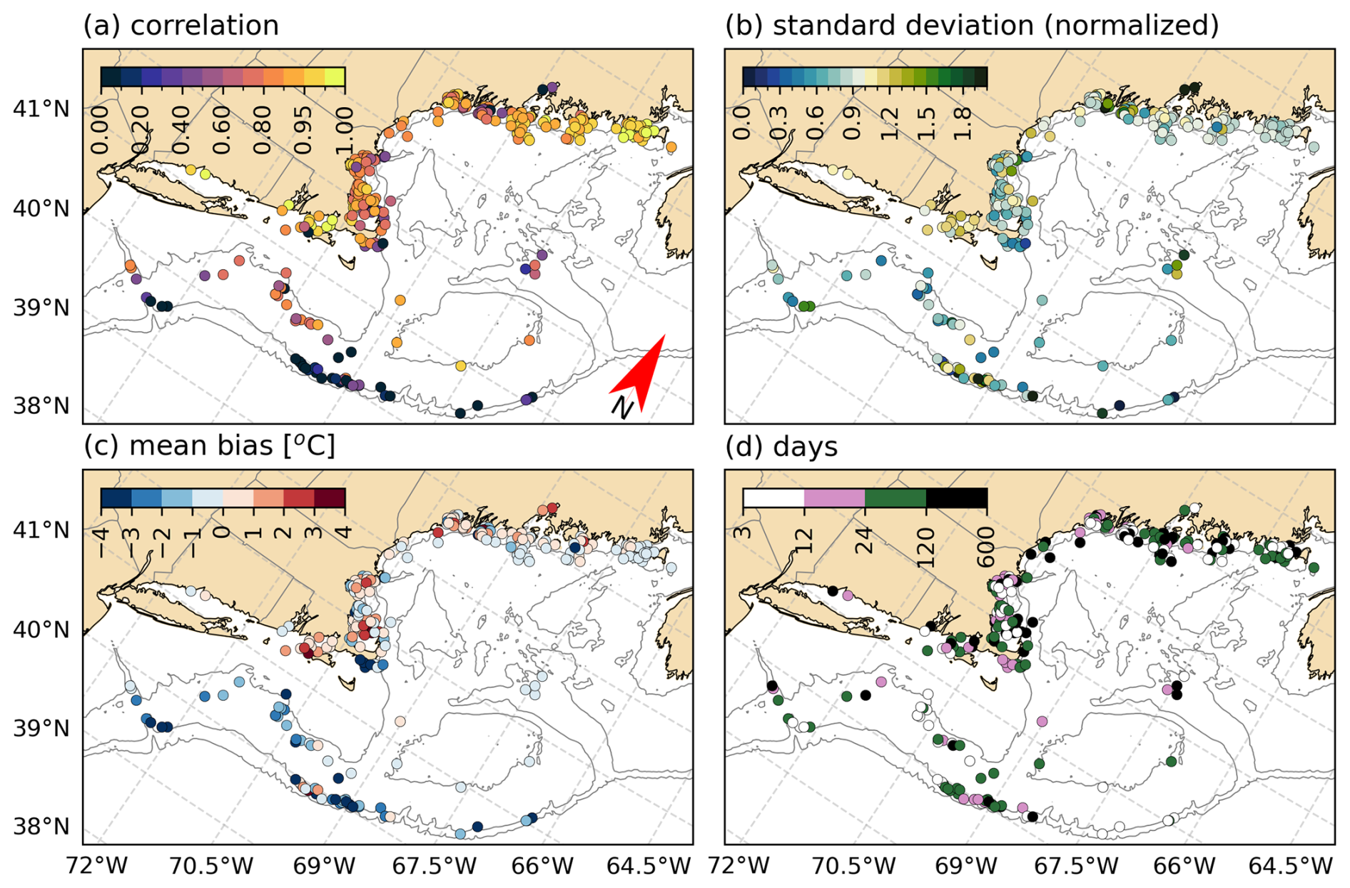
Figure 9 Daily averaged bottom temperature statistics between MOM6 results and eMOLT dataset corresponding to (a) correlation, (b) standard deviation, (c) mean bias and (d) number of days available (log scale). The contours represent depths of 60, 200, and 1000 m.

4.2.3 Seasonal vertical structure

Seasonal climatological profiles based on the World Ocean Database (WOD) were built by calculating the horizontal average of temperature and salinity for each depth using the high-resolution CTD dataset within the different subregions listed in Fig. 1. To ensure statistical robustness, only depths containing more than one hundred points were selected in the profile calculations. Data density varies seasonally, with measurements in the surface ranging from 2000–8000 points in all seasons except for winter, when counts decrease to approximately 1000 points (or less).

Figure 10 presents a comparison between the temperature and salinity profiles of MOM6 and WOD, while skill metrics, such as as bias, MAE, and RMSE are graphically presented respectively in Fig. A4. Depth-averaged bias, MAE, and RMSE suggest better performance in general of MOM6 in the Gulf of Maine for both temperature and salinity relative to GLORYS, while GLORYS better represents these fields in Georges Bank and Mid-Atlantic Bight.

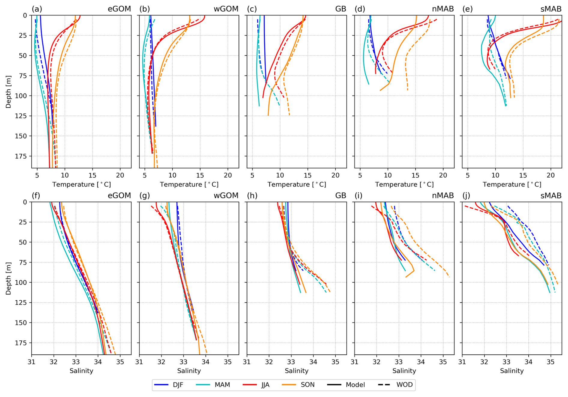
Figure 10 Seasonal profiles of (a–e) temperature and (f–j) salinity on the continental shelf. High-resolution CTDs obtained from the World Ocean Database (solid lines) and MOM6 results (dashed lines).

The seasonal changes of the thermohaline structure across subregions show temperature represents the dominant control on seasonal stratification, with maximum surface values showing during summer and fall (JJA, SON) and minimum in winter and spring (DJF, MAM) (Fig. 10). Seasonal temperature variability influences depths to 150 m in the Gulf of Maine regions (GM: wGOM and eGOM), while affecting the entire water column in the shallower Georges Bank and Mid-Atlantic Bight (GB/MAB: GB, nMAB and sMAB, Fig. 1a).

During warm seasons, a horizontal temperature gradient characterizes the shelf. Average surface temperatures are cooler (approximately 12 °C) in the northeastern areas of the domain and progressively increase southwestward, where maximum seasonal averages occur (24 °C) (Figs. 6, 10). The northeast-to-southeast temperature gradient persists in colder seasons, when eGOM exhibits temperature of about 5 °C, while sMAB shows warmer conditions with temperature near 10 °C (Fig. 10). These patterns reflect the influence of latitudinal surface heating differences and the effects of different water masses on the continental shelf.

The vertical structure can be organized in two distinct regions corresponding to the GM and GB/MAB. Temperature generally decreases with depth down to 75 m in all regions during summer, but GB/MAB depicts a subsurface temperature minimum between 25–80 m depth, below which temperature increases towards the (Fig. 10). This minimum in MAB is compatible with the Cold Pool depths and temperatures. MOM6 generally represents the seasonal structure of temperature in DJF/MAM especially in GM, but underestimates subsurface warming, showing discrepancies up to 5 °C in GB/MAB. These discrepancies are evaluated in Sect. 5.

During fall (SON), the vertical stratification weakens through all domains, with the subsurface minimum disappearing in most of GB/MAB (Fig. 11). Model-observation disparities remain in this season, with the model exhibiting a cold bias of 3–4 °C in deeper areas and underestimating MAB temperatures by approximately 2 °C throughout the water column. Winter (DJF) brings the weakest vertical stratification in all domains, with temperatures increasing towards the bottom. Minimal biases are present in GB and reach −5 °C in nMAB. MOM6 successfully represents the stratification in wGOM, eGOM, sMAB, but shows a warm bias (1 °C) in GB and underestimates the warming at lower levels in nMAB.

Salinity profiles (Fig. 10f to j) show seasonal variability restricted to the upper 50 m in GM and GB, while MAB has pronounced variations throughout the water column. In all regions, salinity values increase toward the bottom, reaching maximums between 34–35 in GM, and 33–36 in GB/MAB. MOM6 reproduces the seasonal profiles of salinity in GM and upper GB, with deviations of salinity of 0.5 in the deepest parts of the water column at wGOM . In deep parts of GB salinity profile, MOM6 underestimates the salinity by 2.0. In MAB, MOM6 is able to reproduce the vertical gradients of salinity but is negatively biased by approximately 1.0 throughout the water column.

4.2.4 Time series evaluation – NERACOOS

The evaluation of temperature and salinity time series between MOM6 results and NERACOOS moorings (Fig. 1) show MOM6-COBALT-NEUS25 generally has a good skill (> 0.95, Willmott, 1981) in representing temperature considering levels shallower than 50 m, with more skill values between 0.75 and 0.9 at depths below 50 m (Fig. 11). In terms of salinity, the model representation is still relatively good, despite the skill approximately between 0.6 and 0.95 when compared with temperature. At upper levels (< 50 m) in all buoys, the model shows better agreement with observations, with correlations ranging from 0.95–0.99 and normalized standard deviation between 0.8 and 1.2.

Buoys M and N, located in deeper regions (> 200 m) in the Gulf of Maine (Fig. 1), generally show a drop in the skill to values between 0.74 and 0.92 when representing temperature time series (Fig. 11). The correlations between measurements and model results range from 0.8 to 0.95 while normalized standard deviation values are between 0.6 to 0.9 for buoy M considering depths below 100 m. At the same levels, buoy N exhibits correlation and normalized standard deviations ranging between 0.6 to 0.8 and 0.7 to 1.2, respectively. Lower correlation coefficients of subsurface series of these moorings is expected since the influence of atmospheric fluxes reduces with increasing depth and depends more on the internal variability of the ocean and the inflow through the Northeast Channel.

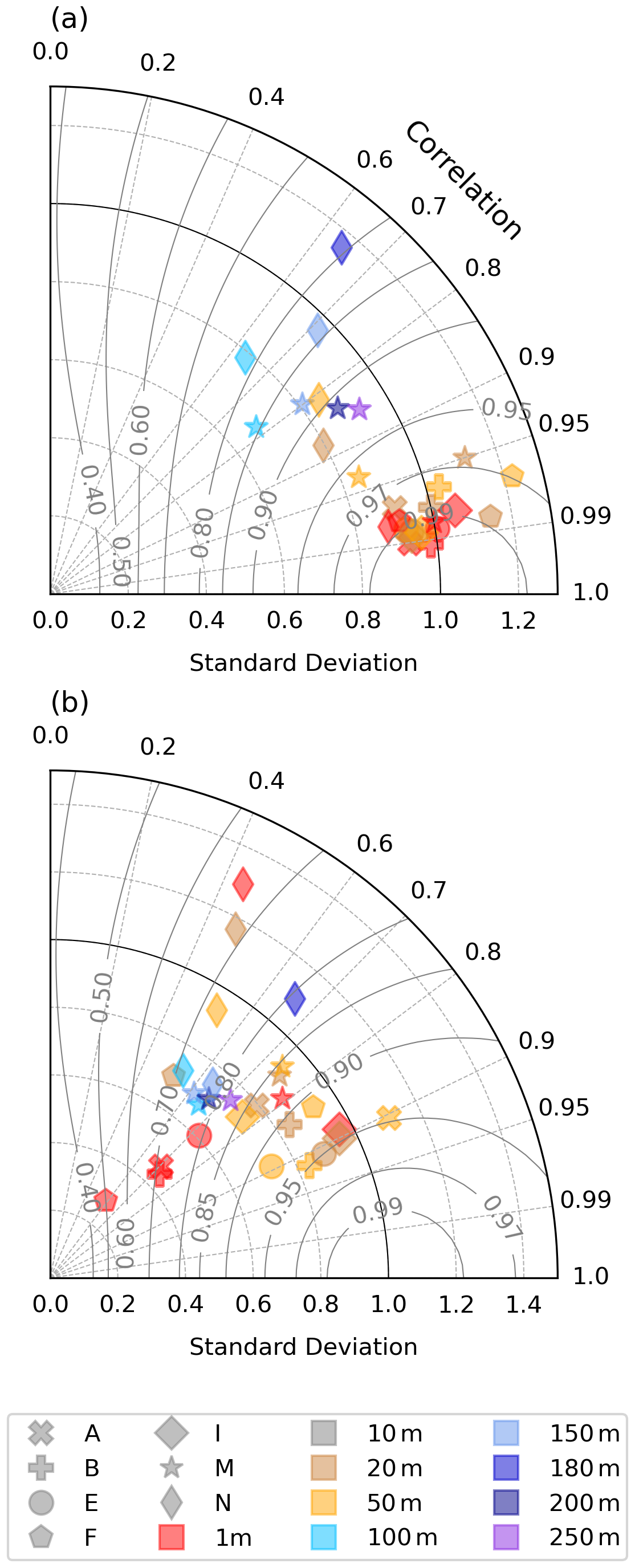
Figure 11 Taylor diagram evaluating MOM6 daily temperature (a) and salinity (b) performance against NERACOOS measurements. Gray shapes in the legend represent the mooring identification, while colors represent measurement depths. The standard deviation of the model results is normalized by the standard deviation of the observations. Curved contours represent isolines of skill score (Willmott, 1981).

The salinity evaluation using Taylor Diagram (Fig. 11b) shows that surface values are not as well represented in MOM6-COBALT-NEUS25, when compared with its temperature counterparts, as correlation coefficients show values of approximately 0.7 and standard deviation below 0.6 for coastal buoys (buoys A to I). These lower skill metrics are likely due to uncertainties in the continental input of freshwater, that force salinity to values below 30 (Figs. A6–A12). Considering depths of 20 and 50 m at coastal buoys, the model has correlation coefficients and standard deviation that are relatively good (0.7 to 0.9, and 0.6 to 1.1, respectively). At buoys M and N, the best representation of the MOM6-COBALT-NEUS25 is related to the depths between 100 to 250 m, with correlation coefficients of approximately 0.6 and typical standard deviation of about 0.7. At these levels, both moorings show systematic biases of salinity (∼ 0.6) and temperature (∼ 1.5 °C).

In general, these metrics are similar to a simulation using a non-structured mesh with resolution of approximately 200 m nearshore and typically of 1 km for the period from 2017 to 2018 (Wang et al., 2022), and to results of a similar coupled hydrodynamic and biogeochemistry model (Lehmann et al., 2009), with MOM6-COBALT-NEUS having better skill in representing levels below 100 m at NERACOOS moorings. This improved representation could be related to the longer simulation period from MOM6-COBALT-NEUS25, which captures the interannual frequency range, as opposed to the shorter simulation of Wang et al. (2022). Global reanalyses (CFSR, ECCO, ORAS, SODA, BRAN, GLORYS, GOFS3.0, GOFS3.1) often have worse skill in representing NERACOOS surface data when compared with MOM6-COBALT-NEUS25 considering the Taylor Diagram metrics (Castillo-Trujillo et al., 2023, Fig. 20).

4.2.5 Interannual evaluation – SST

A comparison between empirical Orthogonal Function (EOF) analysis of SST daily anomalies of MOM6 and OSTIA (Fig. 12) demonstrates that MOM6-COBALT-NEUS25 has good skill in representing the dominant modes of variability in both Gulf of Maine and Mid-Atlantic Bight from 1993 to 2019. The first mode accounts for about 40 % of the explained variance in MOM6 and OSTIA, while the second mode represents about 12 % of the explained variance in both cases.

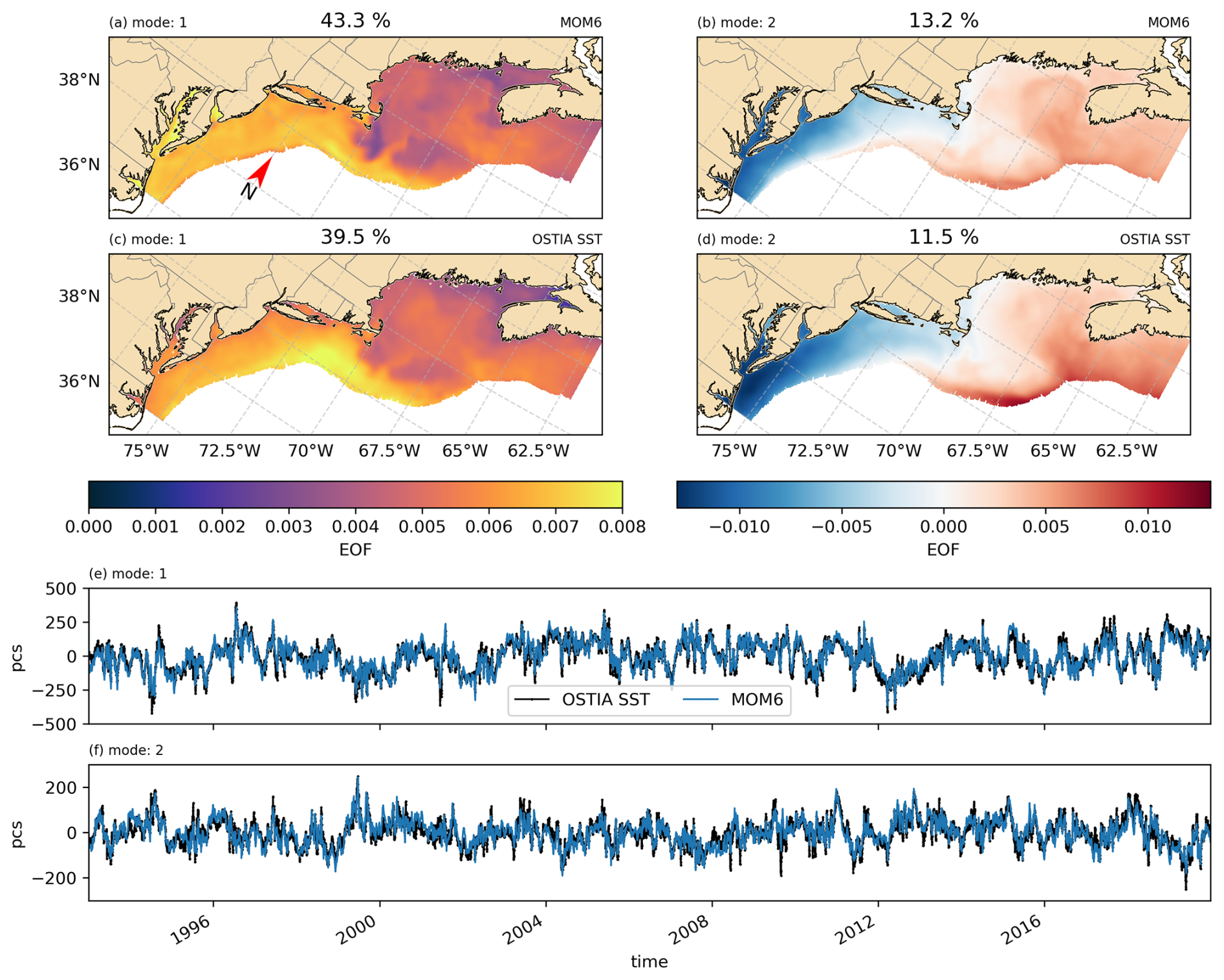
Figure 12 First (a, c, e) and second (b, d, f) modes of empirical orthogonal functions and principal component time series considering SST detrended daily anomalies of MOM6 (a, b) and OSTIA SST (c, d). For the first (second) mode of principal components correlation, normalized standard deviation, mean bias and mean absolute error are 0.94, 1.04, 0.4487, and 167.73 (0.88, 1.02, −0.08, 27.74), respectively. The explained variance of MOM6 (OSTIA SST) first mode is 43.3 % (39.5 %), while the second mode has 13.2 % (11.5 %).

The spatial and temporal patterns of both EOFs are similar in the model and observational product. The first mode (Fig. 12a, c, e) behaves as a monopole with well-marked regional features, including the lower-amplitude signals south of Cape Cod (MA), Georges Bank, and associated with the eastern Gulf of Maine Coastal Current system, where the EMCC steers into the Gulf of Maine at about 44° N near Penobscot Bay (ME). These lower amplitude systems are defined in both MOM6-COBALT-NEUS25 and OSTIA. The second mode (Fig. 12b, d, f) displays a seesaw pattern between the Mid-Atlantic Bight and Gulf of Maine, with MOM6 capturing features associated with the circulation and topography in the Gulf of Maine.

The Principal Components time series (Fig. 12e, f) shows a high correlation between model and satellite measurements for the first and second modes (0.94 and 0.88, respectively). Both modes present relevant variability spanning subseasonal and interannual timescales.

4.2.6 Sea surface height

The sea surface elevation measured by CO-OPS tide gauges were compared with MOM6-COBALT-NEUS25 results for the simulated period starting in 1993, at sites where long term measurements were available (Fig. 1a). To ensure comparison at the same datum, we removed their respective time average values before performing the evaluation presented below. In order to isolate subtidal variability, tidal signals were fitted using harmonic analysis with the U-tide package (Codiga, 2011) and removed from the original time series. The resulting detided signals were filtered using a Lanczos filter with a 24 h cut-off period.

A Taylor Diagram (Fig. 13) summarizes the comparison between observed and modeled sea surface height anomalies, showing generally good agreement. Correlations were ≥ 0.95 at all tide gauges except Woods Hole, where the correlation was approximately 0.7. The normalized standard deviation of the simulated results was approximately 1.0 in the coastal stations of the Mid-Atlantic Bight (Chesapeake Bay, Atlantic City, and New Port), while at Woods Hole, Portland and East Port tide gauges, the normalized standard deviation ranged between 1.05 and 1.35.

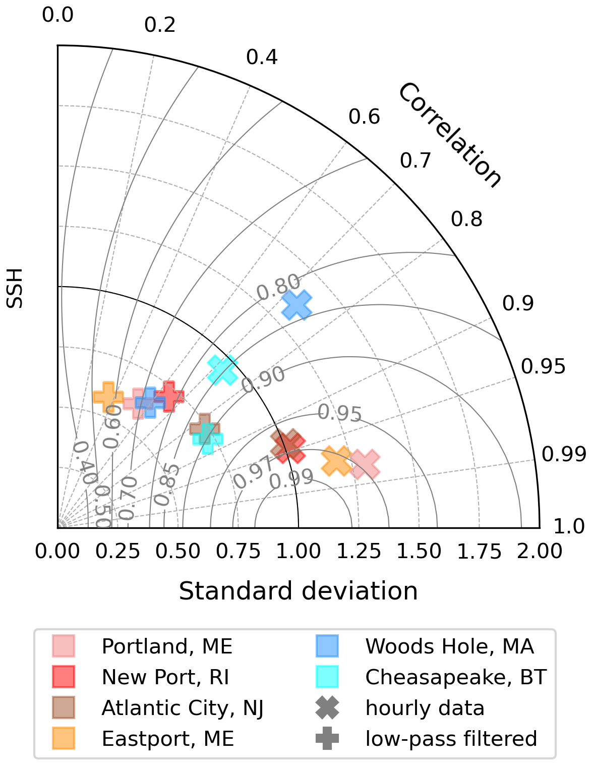
Figure 13 Taylor diagram of hourly SSH data at tide gauges at multiple coastal areas in the Gulf of Maine and Mid-Atlantic Bight alongside low-pass data with a cutoff period of 24 h (Lanczos filter). The standard deviation of the model results is normalized by the standard deviation of the observations. Curved contours represent isolines of skill score (Willmott, 1981).

Detided signal comparisons show reduced correlation (0.4–0.8) (Fig. 13), indicating limited skill of MOM6-COBALT-NEUS25 in representing the subinertial variability and indicating the model skill in coastal sea surface height is driven primarily by the tidal signal. Key factors contributing to reduced skill in representing the subinertial variability include known biases in ERA5 fluxes in coastal areas, where wind forcing tends to be underestimated.

4.3 Biogeochemistry

The seasonal climatology of NO₃ (Fig. 14) was built using the dataset described in Rebuck and Townsend (2014) between the surface and 10 m. This was used to calculate an objective analysis, which finds the best fit of data onto a grid based on decorrelation scales of the data points and their positions. Here, decorrelation scales were determined by fitting a gaussian curve into a semi-variogram. Horizontal data density varies between seasons, with DJF months having the fewest observations (998), followed by SON, with 1548, JJA with 1886, and MAM with the highest data counts (3048) (Fig. 14). The spatial distribution of points does not allow this interpolation to resolve scales under 25 km. While more sophisticated objective analysis approaches exist for continental shelf environments (e.g., Sasaki et al., 2024), our two-dimensional objective analysis provides adequate estimates and enables direct comparisons with the surface krigging derived monthly climatology presented in Rebuck and Townsend (2014).

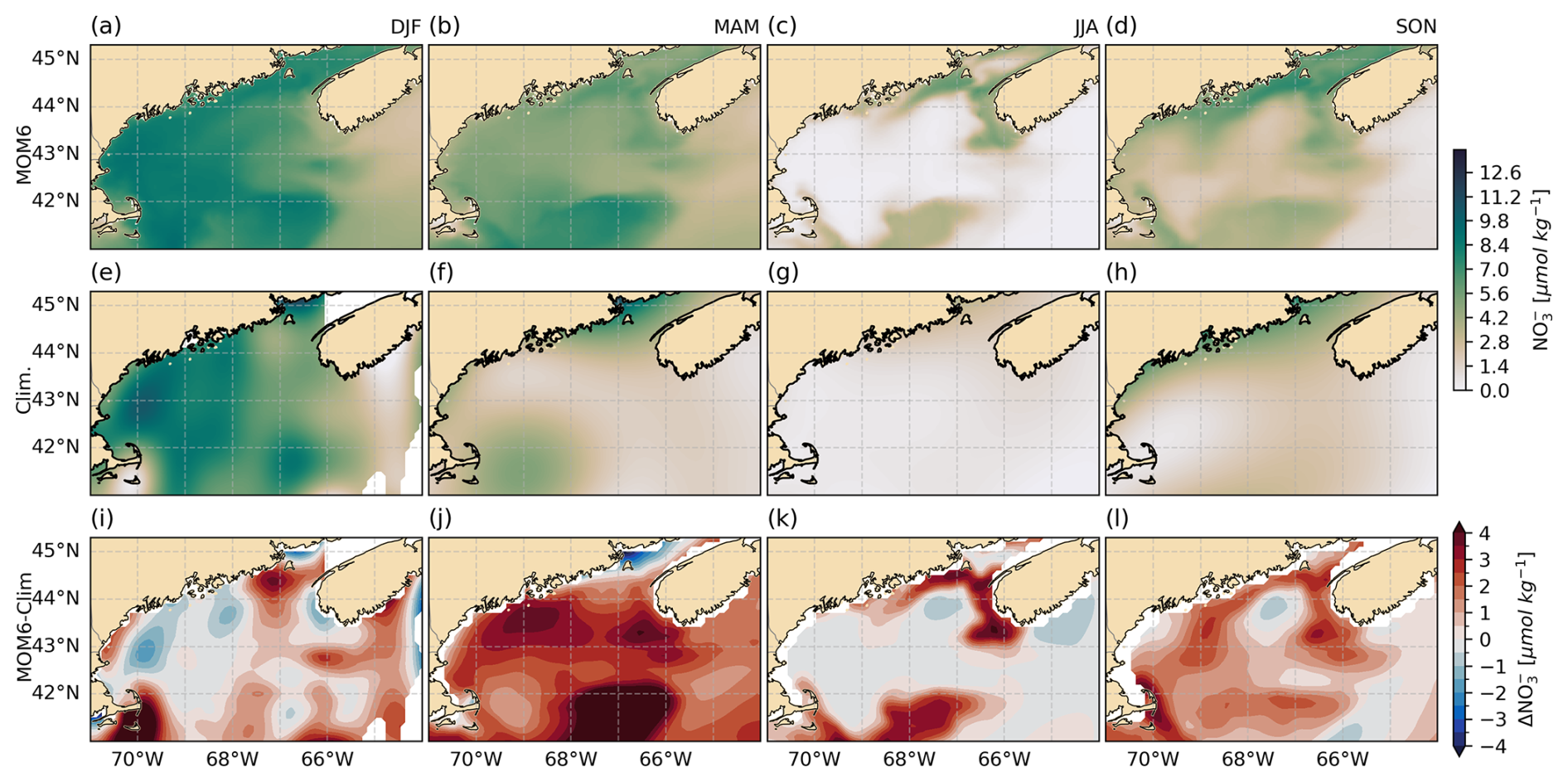
Figure 14 Seasonal surface distribution of nitrate in the Gulf of Maine region considering the climatology of surface concentrations from MOM6 (a–d), a seasonal climatology calculated from Rebuck’s dataset (e–h), and their difference (i–l) (MOM6 – Climatology). Columns represent seasons: DJF, MAM, JJA, SON.

The validation of surface NO₃ concentrations focuses on seasonal cycles and spatial patterns given the inherent uncertainties in the observational climatology due to sparse data coverage. MOM6 simulated surface NO₃ concentrations exhibit the expected seasonal cycle – in areas where the Gulf of Maine is deeper than 200 m, from DJF to JJA, NO₃ surface concentration decreases from about 10.0 to 0.0 µmol kg⁻¹, before rising again from JJA to DJF (Fig. 14). There are asymmetries between transition seasons, with of spring NO₃ averages (8.0 µmol kg⁻¹) showing higher concentrations than fall (4.0 µmol kg⁻¹) . Within the 200 m isobath and near Maine and Nova Scotia coasts, MOM6 shows relatively constant NO₃ surface concentration year-round, maintaining approximately 7.0 µmol kg⁻¹. In contrast, the concentrations of NO₃ along the coast of Massachusetts and New Hampshire align more closely with the climatology, suggesting adequate representation of riverine nitrate inputs.

The largest biases in the model results (Fig. 14i to l) occur during MAM and SON. In Georges Bank, MOM6 surface NO₃ presents higher concentrations (ΔNO₃ ≈ 5.0 µmol kg⁻¹) than in deep regions in Gulf of Maine (> 200 m isobath) during all seasons, except in summer. These patterns are not observed in the climatology, which may suggest enhanced vertical mixing that brings nutrients from deeper layers to the surface at Georges Bank.

While MOM6 and the climatology have similar seasonal magnitudes, the climatology generally shows lower coastal NO₃ values than the model (Fig. 14). These climatological values require careful consideration as discrepancies from the observational seasonal averages arise mainly from two aspects that can be evaluated: first, the heterogeneous data distribution in time and space which may introduce biases; second, the objective analysis prioritizes scales compatible with the decorrelation length, while dampening signals of other scales.

The evaluation of chlorophyll fields (Fig. 15) shows the model has generally lower and more uniform concentrations, with values higher than 1 mg m⁻³ present on the continental shelf, particularly close to the shoreline. In the area corresponding to Georges Bank, OC-CCI shows concentrations higher than 2 mg m⁻³, while MOM6-COBALT-NEUS25 presents values between 1 to 2 mg m⁻³, approximately. These hotspots of higher concentration in the model are present along the coast and Georges Bank, with maximum concentrations of about 2 mg m⁻³ along coastlines from Cape Hatteras up to Delaware, between Rhode Island and Massachusetts and between the coasts of Maine, Bay of Fundy and Nova Scotia. The distribution of chlorophyll in MOM6-COBALT-NEUS25 is very similar to a high resolution model with coupled ROMS and biogeochemistry model at NEUS (Lehmann et al., 2009, Fig. 4).

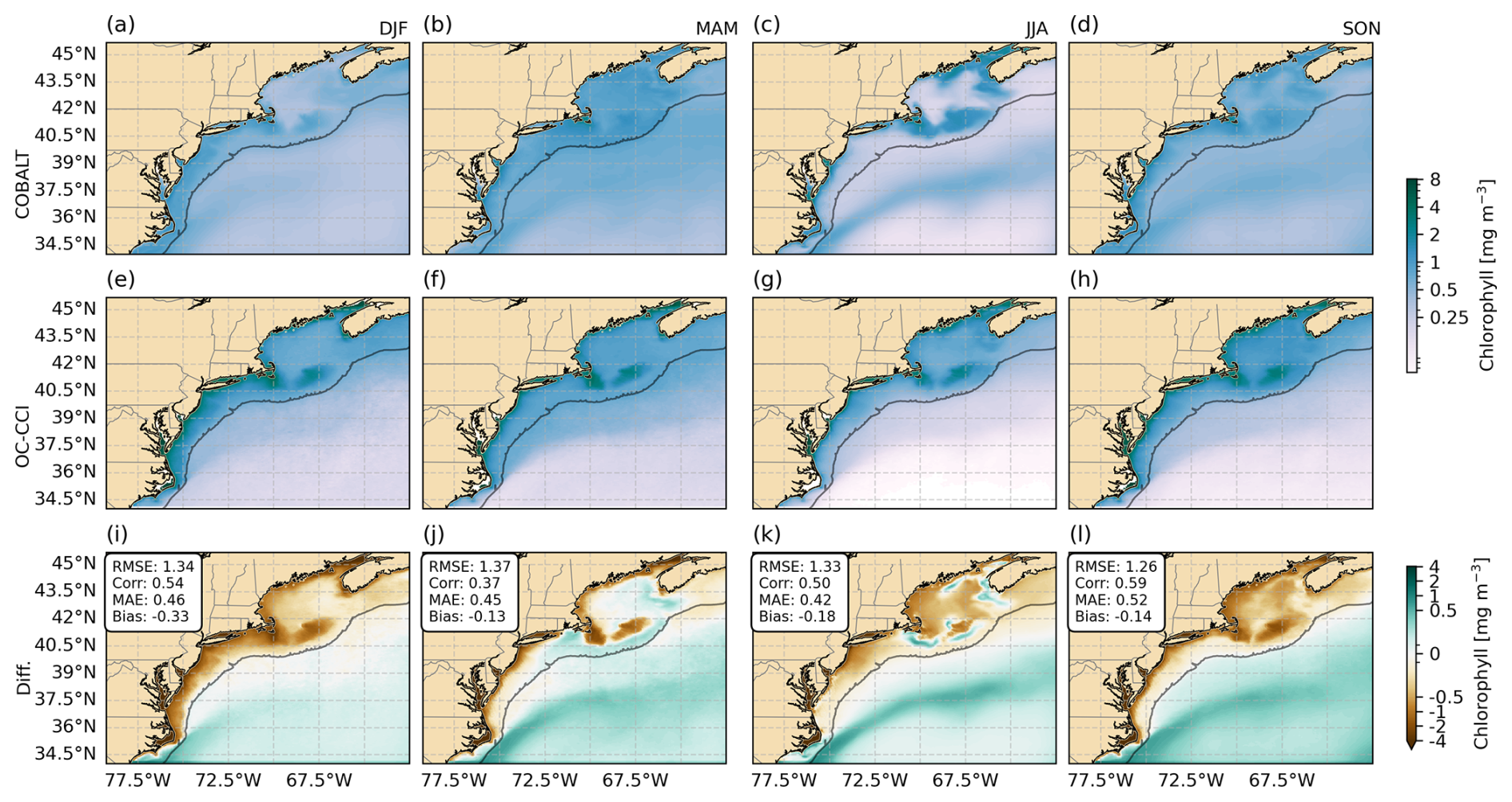
Figure 15 Difference between seasonal averages of surface chlorophyll from MOM6-COBALT-NEUS25 results and OC-CCI satellite data product.

In OC-CCI, two seasonal peaks of chlorophyll are observed in the Gulf of Maine: the first in spring, when concentrations are approximately 1 mg m⁻³, and during fall, when chlorophyll has values between 1 and 2 mg m⁻³, while minima occur in winter and summer (Fig. 15). Similarly, MOM6-COBALT-NEUS25 chlorophyll peaks in spring and fall, but exhibits maximum seasonal concentrations in MAM (1 mg m⁻³) instead of SON (0.5 to 1 mg m⁻³), with minimum values in summer (< 0.25 mg m⁻³). Spatial correlations are relatively low, with values typically close to 0.5, except for spring, when correlation is the lowest (0.38), while the remaining metrics are relatively stable across the seasons for RMSE (∼ 1.3), MAE (∼ 0.45) and Bias (−0.13, with exception of DJF −0.33).

In the slope, MOM6-COBALT-NEUS25 presents spurious higher chlorophyll concentrations associated with the Gulf Stream (Δ Chlorophyll 0.5 mg m⁻³, Fig. 15i to l). The phytoplankton boundary conditions in MOM6 are provided by a long-term climatology of a global COBALT simulation (Stock et al., 2014), which was also used in R23. The difference between R23 and MOM6-COBALT-NEUS25 lies in the turnover times of phytoplankton association with the boundary conditions. In our case, differently from R23, the Gulf Stream introduces fast currents (> 2.0 m s⁻¹ in some cases which does not allow phytoplankton to equilibrate during summer with the seasonality of macronutrients (such as nitrate) inducing the jet-like phytoplankton feature seen throughout the year, which is more apparent in the summer fields. A second aspect that could be an issue is the lower resolution of 1° (∼ 100 km) in global COBALT, which doesn't resolve the gradients associated with the shelf-slope continuum.

Seasonal and monthly gridded depth-average measurements of mesozooplankton carbon biomass on the continental shelf available from the COPEPOD database are used in the evaluation of mesozooplankton fields of MOM6-COBALT-NEUS25 (Fig. 16). The monthly boxplots represent the horizontal distribution of monthly and depth-averaged carbon biomass of the upper 200 m. Because the gridded COPEPOD dataset does not provide sample counts per grid point, we avoid formal correlation or skill metrics and instead use boxplot analysis for quantitative comparison (Fig. 16c). Model and observations agree on the broad seasonal cycle, with average concentration below 10 mgC m⁻³ during the winter (DJF) and fall (SON), rising to 20 mgC m⁻³ over spring (MAM) and summer (JJA). Monthly averages from April to August reach 20 mgC m⁻³ in the observations, which is higher compared with model values of 15 mgC m⁻³. The spatial distribution of the model has an interquartile range around the median of about ±5 mgC m⁻³, contrasting with the observations’ range of about ±20 mgC m⁻³ from mid spring (MAM) to early fall (SON).

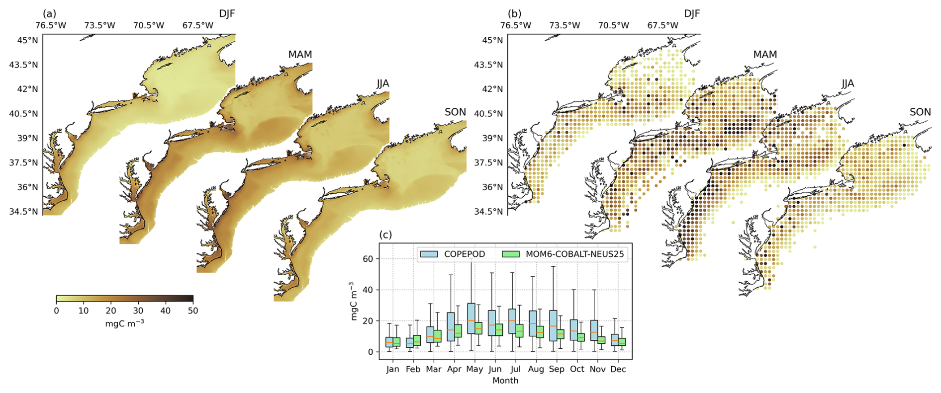
Figure 16 Seasonal averages carbon biomass (depth-averaged over the top 200 m) on the continental shelf (within the 400 m isobath) encompassing the Mid-Atlantic Bight, Georges Bank and Gulf of Maine for (a) MOM6-COBALT-NEUS25, and (b) COPEPOD dataset. Boxplots represent the distribution of the horizontal fields of monthly and depth-averaged biomass. Seasonal bias are (DJF, MAM, JJA, SON) (1.3, 5.7, 7.2, 10.9) mgC m⁻³.

In the Gulf of Maine, simulated depth-averaged mesozooplankton biomass is underestimated in regions beyond the isobath of 80 m (Fig. 16a, b), with concentrations varying from less than 5 up to 15 mgC m⁻³, while COPEPOD suggests values generally over 15 mgC m⁻³. Concentrations in the Mid-Atlantic Bight are approximately 20 mgC m⁻³ in spring and summer (JJA), with lower values between 5 to 20 mgC m⁻³ in winter (DJF) and fall (SON). COPEPOD has similar values, but some hotspots in the observations are absent from the model results. These hotspots occur mainly at Georges Bank in MAM (spring) and coastal areas along Chesapeake and Delaware Bays during summer (JJA), where the biomass concentrations reach values higher than 40 mgC m⁻³.

In general, the model captures the seasonal and spatial patterns while underestimating possible regional maxima. The underestimates in the model could be related to the mesozooplankton size that is represented. Our results contrast with R23 evaluation of mesozooplankton, who multiplied COPEPOD biomass estimates by a factor of two due to the different fraction sizes represented in COBALT (200–2000 µm), relative to COPEPOD’s biomass adjustment to a 333 µm mesh. Here, we make no such correction, and the observed and modeled values correspond to their respective size fractions rather than following R23's approach.

The boxplot of monthly climatological anomalies relative to the total period of dissolved inorganic carbon (DIC) in the upper 10 m of the water column for the entire domain are shown in Fig. 17. Removing the average DIC is required for the evaluation of the model results, since boundary conditions were derived from the static WOA climatology without a year adjustment in contrast to R23, leading to the magnitude differences in Fig. 17b, c. In these panels, the relevant information is associated with the horizontal gradients that increase in the offshore direction in both model results and the reference climatology. The larger spread around the median (Fig. 17a) in the model reflects the 4 km resolution with a number of points of O[10⁵], compared with the horizontal resolution of about 100 km in Broullón product. The seasonal cycle maps are included in Fig. A13.

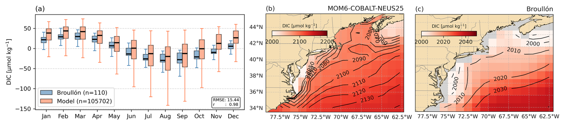
Figure 17 Monthly DIC anomalies in the upper 10 m relative to the long-term monthly mean for MOM6-COBALT-NEUS25 and Broullón (a), where n is the number of horizontal grid points in each dataset. Long-term mean DIC in the upper 10 m over the full period for MOM6-COBALT-NEUS25 (b) and Broullón climatology (c) (background colors). The model results were coarsened to the same resolution as the climatology. Black contours represent the DIC isolines and gray color represent areas where data was not available.

An evaluation between the long-term average of TA in MOM6-COBALT-NEUS25 and an observation-based climatology (Jiang et al., 2021; Jiang et al., 2022) (Fig. 18) shows similar spatial structure in both fields (spatial correlation is approximately 0.9) with horizontal gradients of TA increasing in the offshore direction. The model's average bias is approximately 88 µmol kg⁻¹ in TA. The largest biases are associated with the Gulf Stream and Slope Sea domains. The lowest TA values occur in Chesapeake Bay and surrounding continental shelf. The lowest difference value in Fig. 18c south of Chesapeake Bay is a consequence of the high resolution of MOM6-COBALT-NEUS25, which partially represents coastal inlets. These inlets are associated with freshwater inflow, which introduces low TA values in the surrounding continental shelf.

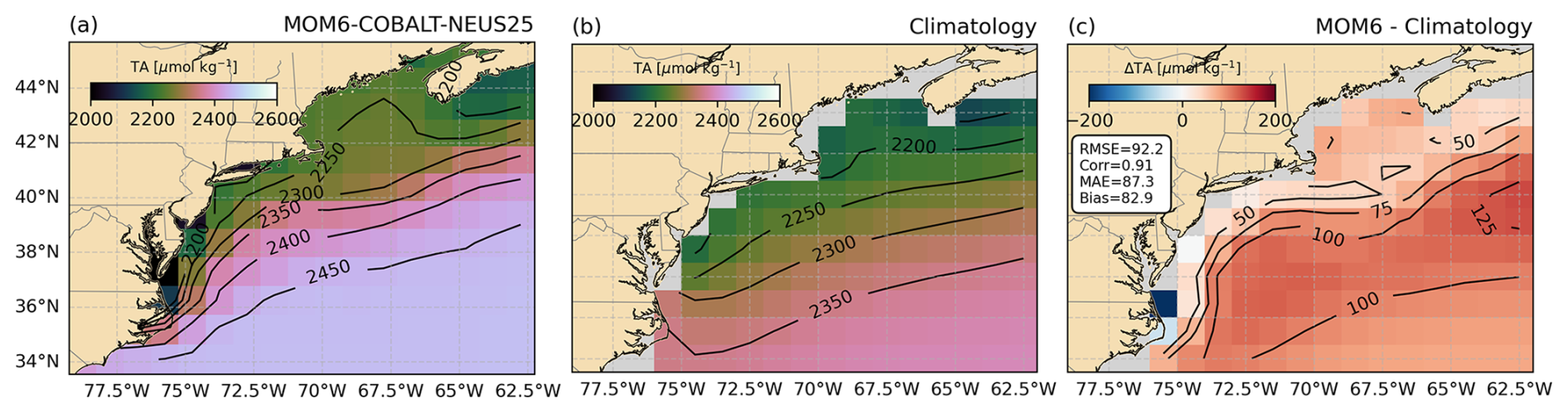
Figure 18 Long term average of total alkalinity (TA) considering MOM6-COBALT-NEUS25 (a), the observation-derived climatology (b), and their difference (c). TA field in the model was binned (and averaged) into the same resolution as the climatology with a resolution of 1°.

5 Discussion

MOM6-COBALT-NEUS25 demonstrates strong skill in reproducing SST variability across the continental shelf at both seasonal and interannual timescales (Figs. 6, 12). This performance indicates the model appropriately represents the region's dominant SST drivers, which are primarily surface heat fluxes (Li and He, 2014). The consistency between our model EOF patterns and those from satellite information, particularly their resemblance to the seasonal EOF structure documented by (Li and He, 2014), suggests the model captures the fundamental physical processes controlling temperature variability in this region, with heat flux forcing and vertical mixing dominating over advective processes at these temporal scales.

While early measurements and analysis (1979–1987; Mountain et al., 1996) indicated heat fluxes were relevant at interannual scales, the eastern Gulf of Maine SST was dominated by advective changes. Different factors could contribute to this apparent difference relative to our model results. First, observational coverage has evolved substantially since the 1980s and presently benefits from comprehensive satellite coverage. Second, physical changes in the Gulf of Maine (Townsend et al., 2010) could have had substantial impacts on circulation, leading to more uniform SST variability across the Gulf of Maine

In the Coast of Maine, Nova Scotia and Georges Banks, positive biases present in GLORYS (Fig. A1) are generally absent from MOM6-COBALT-NEUS25. GLORYS reanalysis does not resolve tides, which is relevant for strong nonlinear currents in Nantucket Shoals and Georges Bank (Chen et al., 2011). The observed differences in SST likely reflect physical processes rather than model biases, as tides enhance vertical mixing and generate residual currents in shallow regions with steep bathymetric gradients in the region (Chen et al., 1995; Xue et al., 2000), which mix colder deeper water with the upper layers of the ocean. Furthermore, satellite SST products often misrepresent or exclude data from regions with strong tidal mixing and coastal upwelling, as these signals are frequently flagged as poor quality (Pereira et al., 2020; Murphy et al., 2021). Further analysis is required to validate the SST in these tidally active region, but the model strong overall SST skill suggests it captures the net regional heat budget appropriate for present conditions.

Representing the Gulf Stream separation enabled MOM6-COBALT-NEUS25 to capture the shelf-slope environment, as shown by timeseries of NERACOOS moorings in the Gulf of Maine. A possible explanation for cold and fresh biases below 100 m in Northeast Channel and Jordan Basin, in moorings M and N, may be linked with the model tendency to damp the Gulf Stream meanders, which reduces warm core ring formation. Warm rings introduce Warm Slope Water into Jordan Basin through the Northeast Channel (Du et al., 2022) and with fewer warm core rings, the colder and fresher Labrador Slope Water becomes more dominant in the deep Gulf of Maine, leading to the simulated cold/fresh bias.

In the Gulf of Maine, the seasonal vertical structure and bottom temperatures showed good agreement with observations, contrasting with Georges Bank and the Mid-Atlantic Bight, where skill is more limited, particularly in levels below 50 m. The model represents the Cold Pool – the bottom-trapped cold water mass (temperature < 10 °C, salinity < 34) that originates in the Gulf of Maine and persists in the Mid-Atlantic Bight during summer and fall (Fairbanks, 1982; Chen and Curchitser, 2020). In the Mid-Atlantic Bight, bottom temperatures in areas shallower than approximately 40 m show positive biases during JJA and SON, while a persistent cold bias occurs beyond the 80 m isobath. Varying bottom boundary layer efficiency (bbl_effic) parameters indicated that warm bottom biases within the 40 m isobath during summer and fall are insensitive to bbl_effic changes, contrasting with deeper regions where the biases were reduced. One possibility is that these shallow biases could be linked with insufficient vertical resolution in the z^*-coordinate.

In the Mid-Atlantic Bight, Georges Bank, and Gulf of Maine, SST and surface chlorophyll patterns have an inverse relationship, where cold temperatures are usually linked with higher chlorophyll concentrations (Yoder et al., 2002). This relationship reflects the replenishment of nutrients in the surface through vertical mixing, which is facilitated by less stratified environments. Seasonal SST fields and surface chlorophyll in MOM6-COBALT-NEUS25 are in agreement with observed patterns, with colder temperatures and higher chlorophyll concentrations in the EMCC, Georges Bank, and the region south of Cape Cod. Biases on the continental shelf are difficult to assess, as chlorophyll estimates from satellite measurements present uncertainties related to the ocean color, which does not depend on the concentration of phytoplankton and chlorophyll alone, particularly in coastal regions (Dierssen, 2010).

The salinity in MOM6-COBALT-NEUS25 generally represents the seasonal cycle of SSS relative to the high-resolution NCEI regional climatology (Seidov et al., 2018, 2019), model represent generally the salinity variability measured by the NERACOOS buoys. An evaluation of eight distinct reanalysis (Castillo-Trujillo et al., 2023) show that models with low resolution (0.25°) generally overestimates the salinity climatology over the entire sMAB with bias typical greater than 1.5, while the Gulf of Maine shows negative biases of approximately −0.6. Higher resolution reanalysis (< 0.1°) are generally better in representing salinity with absolute bias usually lower than 0.5. In the NEUS domain, R23's mean surface salinity show biases spread along the shelf from Cape Hatteras to the Gulf of St Lawrence that is attributed to mild issues in The Gulf Stream representation.

A realistic Gulf Stream path in MOM6-COBALT-NEUS25 assessed using SSH standard deviation, is in agreement with satellite observation. Biases in SST and SSS in the Slope Sea are reduced when compared with coarser resolution models (e.g Saba et al., 2016; Ross et al., 2023). Beyond the high resolution, this is possibly also a consequence of the more restricted domain in MOM6-COBALT-NEUS25, where the open boundary conditions and rim nudging have a stronger influence on the mean state, while potentially suppressing internal variability. Considering the Gulf Stream evaluation through SSH standard deviation, it is worth mentioning that the effective resolution of the CMEMS SSH product is about 200 km at mid latitudes (Pujol et al., 2016), which does not resolve the first baroclinic radius in the model domain (Hallberg, 2013; Chelton et al., 1998). The SSH biases in the Slope Sea likely reflect excessive dissipation of turbulent EKE in the current model configuration, or an influence of the nudging close to the boundaries. Despite recent improvements in the representation of SSH in coastal regions in CMEMS SSH (Sanchez-Román et al., 2023), the usage of CO-OPS tide gauges is desirable in the evaluation of tidal variability and subinertial variability in the coastal zone.

In the Gulf of Maine during summer and fall, MOM6-COBALT-NEUS25 underestimates surface chlorophyll concentration. This contrasts with other regional coupled ocean dynamics and biogeochemistry models, such as the Atlantic Canada Model (ACM; Brennan et al., 2016; Rutherford and Fennel, 2018), which better represent surface chlorophyll in the Gulf of Maine during these seasons (Laurent et al., 2021). MOM6-COBALT-NEUS25 and ACM have different domains, with ACM extending from the Massachusetts coast to Newfoundland and Labrador. These different domains allow ACM more realistic biogeochemical fluxes through the Nova Scotia shelf into the Gulf of Maine compared with MOM6-COBALT-NEUS25. Improving boundary condition estimates with well-constrained machine learning methods such as ESPER (Carter et al., 2021) could potentially address these issues, although formal experiments are required.

The seasonal cycle of surface chlorophyll from OC-CCI and depth-averaged mesozooplankton do not coincide, which is expected as mesozooplankton concentration is coupled not only with surface spring and fall blooms, but also with a widespread chlorophyll subsurface maximum that has 2 to 8 times the concentration of the overlying and underlying waters during summer (O'Reilly and Zetlin, 1998). Since MOM6-COBALT-NEUS25 captures this summer subsurface maximum (not shown), the model successfully reproduces the seasonal and monthly structure of depth-integrated mesozooplankton biomass throughout the year, demonstrating its capability to represent key ecosystem dynamics beyond surface processes.

Our results show that MOM6-COBALT-NEUS25 reproduces the seasonal cycle of DIC broadly consistent with the Broullón climatology (Broullón et al., 2020a). The increased resolution and process-oriented design of numerical models allow a better representation of cross-shelf gradients compared with the climatological product. Despite MOM6-COBALT-NEUS25 showing a realistic Gulf Stream path, the mean DIC remains 30–50 µmol kg⁻¹ higher, suggesting the offset is primarily driven by the boundary conditions without a interannual adjustment rather than differences in physical circulation. The cross-shelf gradients agree with observational evidence in the Mid-Atlantic Bight (Li et al., 2024), where nearshore surface waters show DIC concentrations below 2000 µmol kg⁻¹ and offshore waters near the shelf break reach approximately 2050 µmol kg⁻¹. TA fields in MOM6-COBALT-NEUS25 have spatial patterns similar to what was observed in R23 results and the climatology product (Jiang et al., 2022), with the systematic bias in the Gulf Stream being a common feature in both model results. The sensitivity of the TA field to the OBC relaxation parameters (obc_lfac_in = 0.03, obc_lfac_out = 1.0), inherited from the configuration of R23, was not explored in this study and may contribute to the systematic bias. The biases in both DIC and TA mean state share a common origin in the boundary condition configurations.

6 Conclusions

MOM6-COBALT-NEUS25 is now part of a growing group of ocean-biogeochemistry models for the Northeast U.S. Shelf, offering advantages through its MOM6-COBALT infrastructure that is part of the CMIP framework. This coupling enables the regional detail required for shelf-specific applications including mCDR assessments, benthic modeling, hypoxia prediction, and fisheries evaluation. The model demonstrates particular skill in the Gulf of Maine and upper water column processes across the domain, making it suitable for studies requiring accurate representation of seasonal stratification and tidal mixing.

The model skill in the Gulf of Maine is also a consequence of the representation of the Gulf Stream position and the Slope Sea conditions, which constrain the regional circulation. Surface fields (SST, SSS, and SSH) are well constrained relative to observations across the domain. Vertical structure validation reveals regional contrasts: the Gulf of Maine shows good agreement throughout the water column, while the Mid-Atlantic Bight exhibits biases below 50–70 m, particularly during spring and fall. A relevant finding is that the bottom boundary layer efficiency parameter (bbl_effic) affects bottom temperature biases only in waters deeper than 40 m, suggesting that vertical resolution limitations may control errors in shallower regions. Cold SST patches near Nantucket Shoals and Georges Bank, absent in global reanalyses, are realistic and associated with tidally-induced vertical mixing. Surface chlorophyll concentrations and zooplankton representation are on par with remote sensing and observations.

Improving the boundary condition implementation, including time-varying ESPER-derived TA and DIC with an annual adjustment following R23, would reduce the mean state bias but is unlikely to be sufficient for quantitative carbonate chemistry applications in this region without further regional optimization. Validation against in situ carbonate chemistry observations in the Mid-Atlantic Bight and Gulf of Maine will be required before the model can be applied to ocean acidification or carbon budget studies.

MOM6-COBALT-NEUS25 largely benefits from the open community approach of model development established in the MOM6 community and particularly in Ross et al. (2023). Some limitations are clear in the model results. Relevant biases in temperature and salinity persist in vertical profiles below 50 m in summer and fall in the Mid-Atlantic Bight and Georges Bank. In regions shallower than 40 m, bottom temperatures are overestimated in the Mid-Atlantic Bight, which remains unresolved in the current configuration. On the biogeochemical fields, boundary conditions play an important role in the relatively restricted model domain and deserve careful attention in future modeling efforts. Future improvements in the parameterization choices related to vertical mixing in the bottom boundary layer, improved biogeochemical lateral fluxes, and perhaps a more appropriate vertical coordinate on the continental shelf (sigma-coordinates) may reduce biases in the water column structure, bottom temperature, and the representation of surface chlorophyll fields in summer and fall. If successful, these improvements would allow future evaluations to be extended to the entire water column outside of the Gulf of Maine and support a more comprehensive description of the biogeochemistry.

Appendix A: Additional material

Jean-Michel et al. (2021)Hersbach et al. (2020)Egbert and Erofeeva (2002)Harrigan et al. (2021)Garcia et al. (2024b)Dunne et al. (2020)Gomez et al. (2023)Carter et al. (2021)Meinshausen et al. (2020)Stock et al. (2014)

Table A1 Initial conditions, boundary conditions and surface forcing datasets, variables and references.

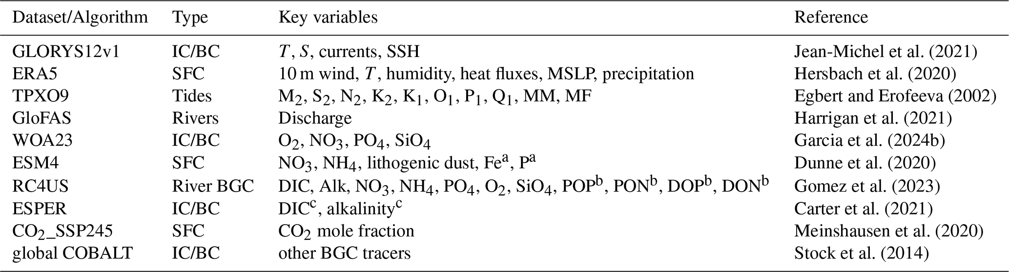
IC = initial conditions; BC = boundary conditions; SFC =  surface forcing; MSLP = mean sea level pressure; T = temperature; S = salinity; SSH = sea surface height; O₂ =  dissolved oxygen; NO₃ = nitrate; NH₄ = ammonium; PO₄ = phosphate; SiO₄ = silicate; Fe = iron; DIC = dissolved inorganic carbon; Alk = alkalinity; DON = dissolved organic nitrogen;POP = particulate organic phosphorus; PON = particulate organic nitrogen; DOP = dissolved organic phosphorus; DON = dissolved organic nitrogen; P = phosphorus; BGC =  biogeochemic. ^a Fe is assumed to be 3.5 % of the dust, Phosphorus is assumed to be 564 ppm of the dust. ^b 50 % of particulate phosphorus is assumed to be buried in estuaries, DON and DOP are fractionated into labile (40 %) semi-labile (30 %), and semi-refractory (30 %). ^c Derived from temperature and salinity using ESPER algorithm. All information is detailed in Ross et al. (2023).

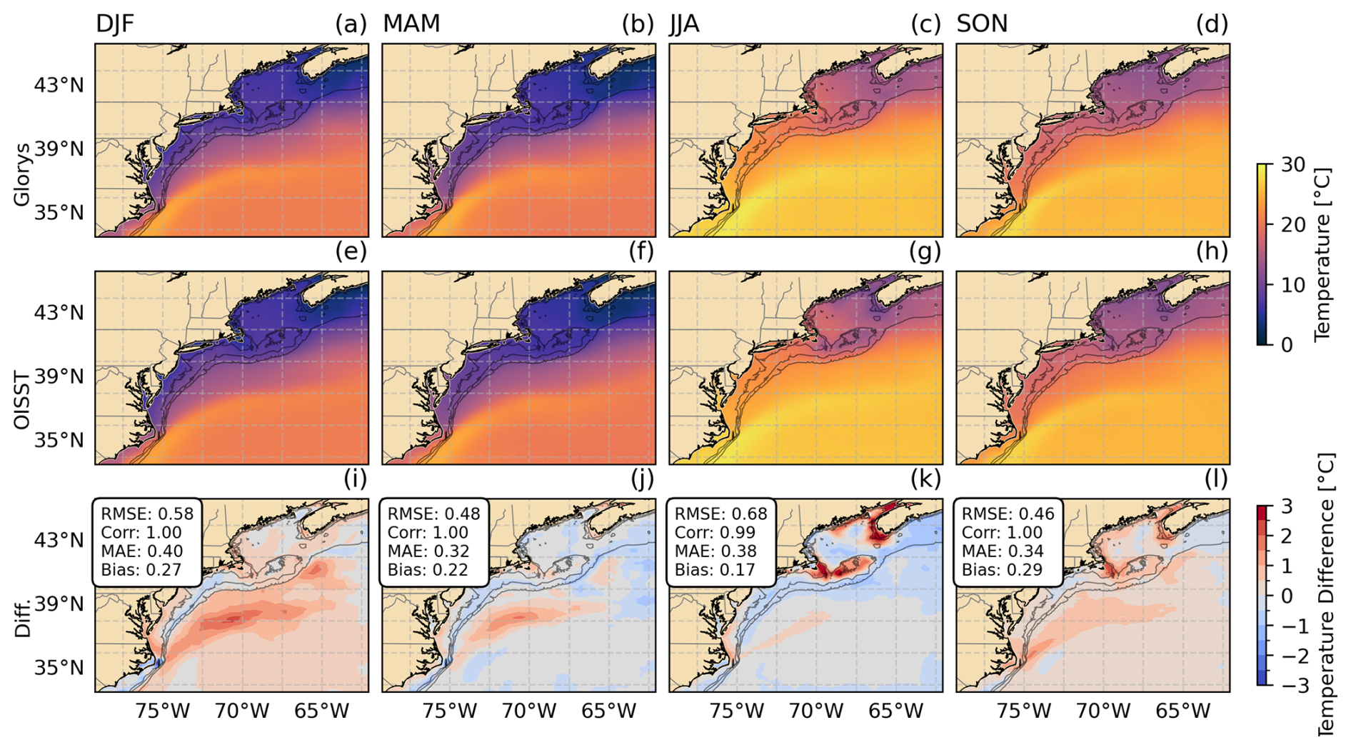
Figure A1 Seasonal averages of sea surface temperature considering GLORYS (a–d), OSTIA SST (e–h) and their differences (i–l, GLORYS – OSTIA). GLORYS results and OSTIA SST were interpolated (bilinear) to MOM6 resolution. Black contours are the isobath of 40, 80, and 400 m.

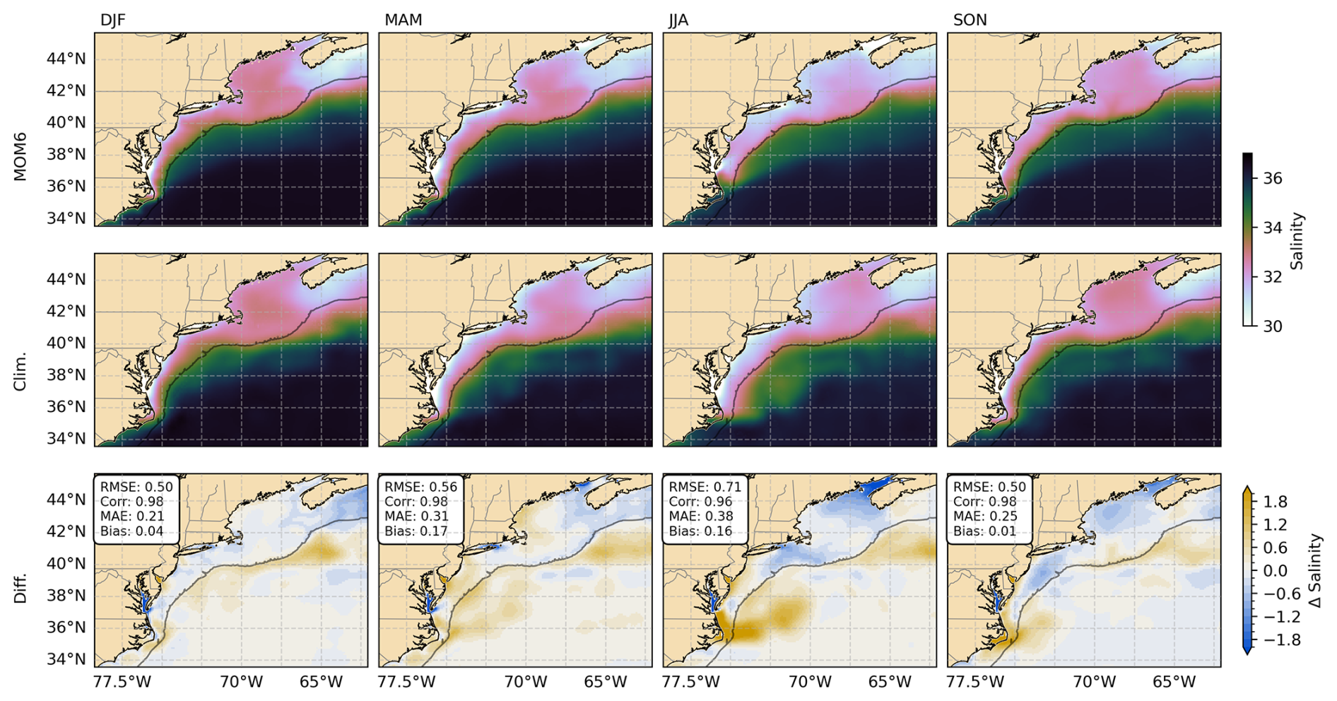
Figure A2 Seasonal averages of sea surface salinity from GLORYS (top panels) and NCEI regional climatologies (Clim., middle panels) and seasonal differences (lower panels, GLORYS – Clim.). Black contour indicates the 400m isobath, roughly representing the position of the shelf break. GLORYS results were upscaled to NCEI climatologies resolution (0.1°) by binning corresponding areas and calculating averages.

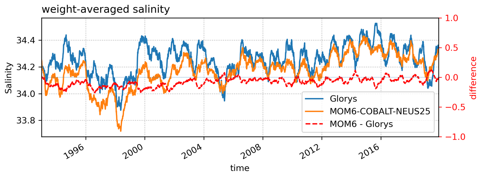
Figure A3 Weight-averaged salinity considering the domain of this study area. The time series show the salinity drift of MOM6-COBALT-NEUS25, GLORYS and their differences.

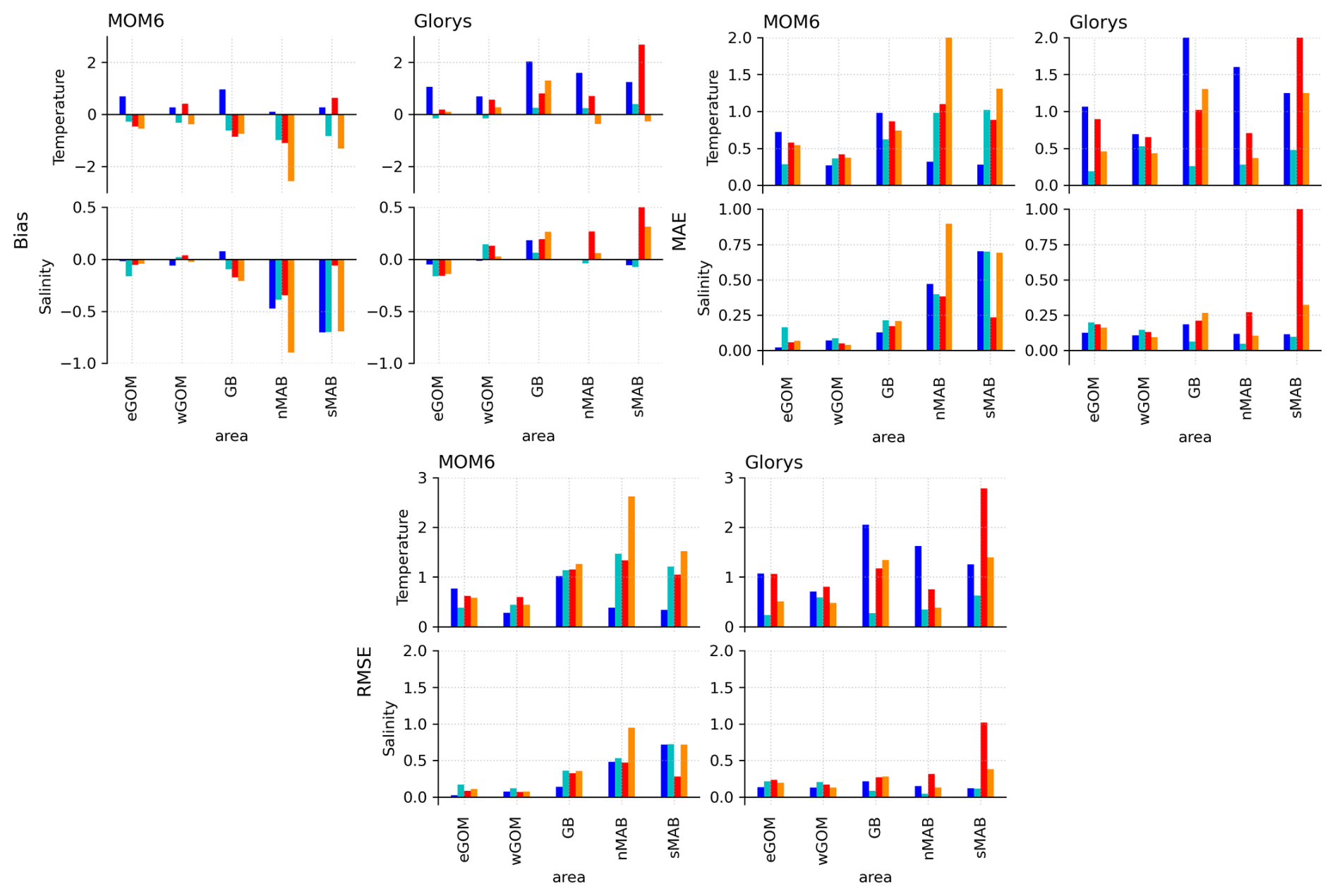
Figure A4 Error statistics of seasonal average profiles at different subdomains of the model. Colors represent winter (blue), spring (cyan), summer (red), and fall (orange)

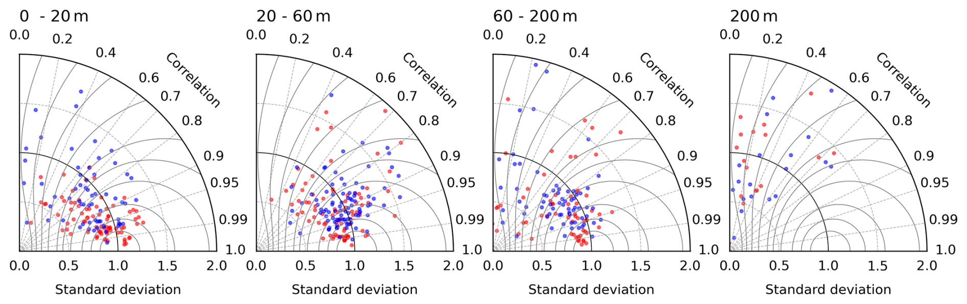
Figure A5 Taylor Diagrams of bottom temperature measurements in lobster thermistors at different bathymetry intervals considering MOM6 (red) and GLORYS (blue) results.

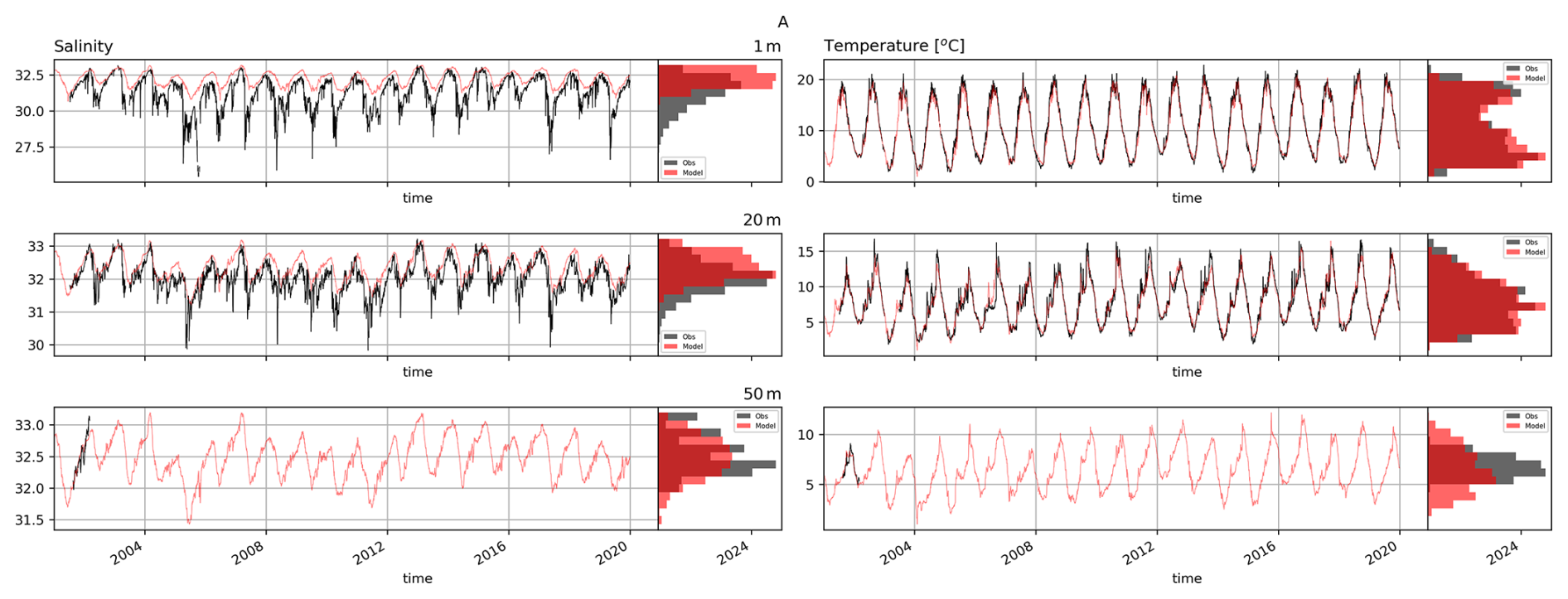
Figure A6 Time series of salinity in temperature of MOM6 (red) and NERACOOS mooring measurements (black) at buoy A.

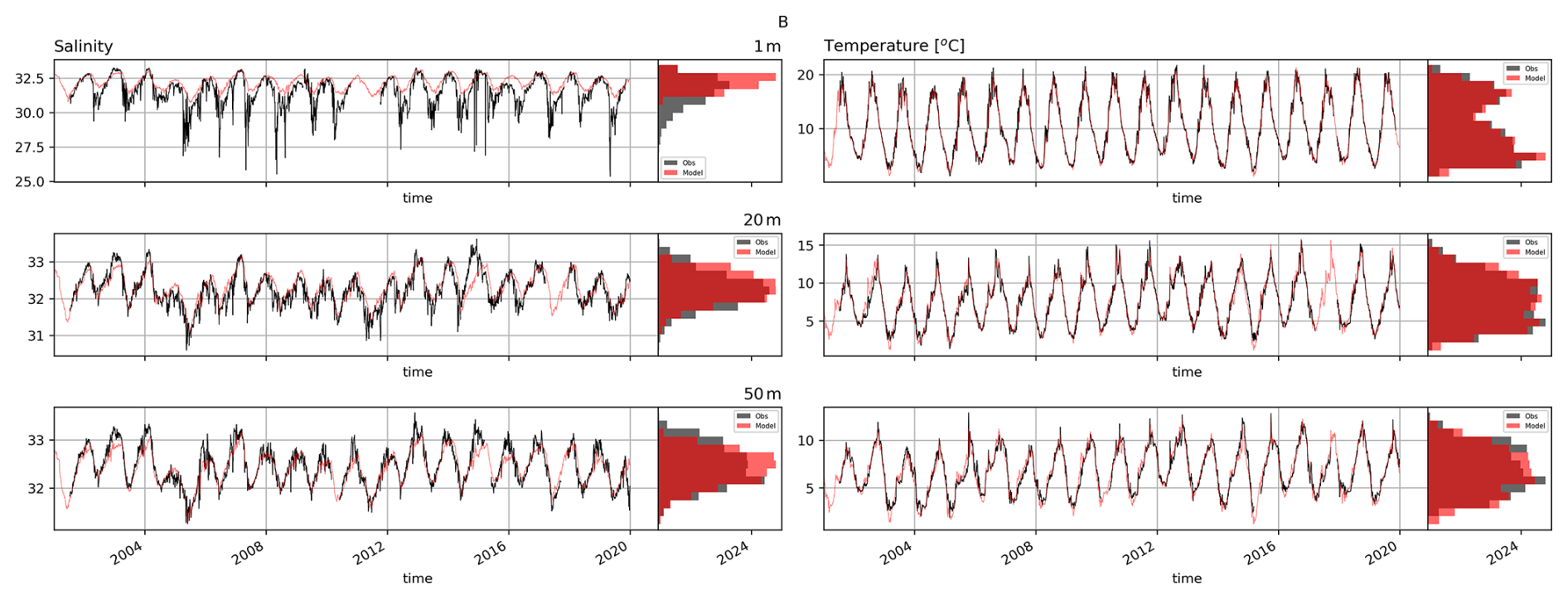
Figure A7 Time series of salinity in temperature of MOM6 (red) and NERACOOS mooring measurements (black) at buoy B.

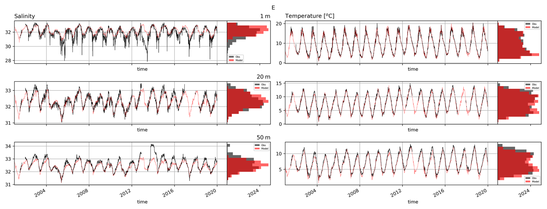
Figure A8 Time series of salinity in temperature of MOM6 (red) and NERACOOS mooring measurements (black) at buoy E.

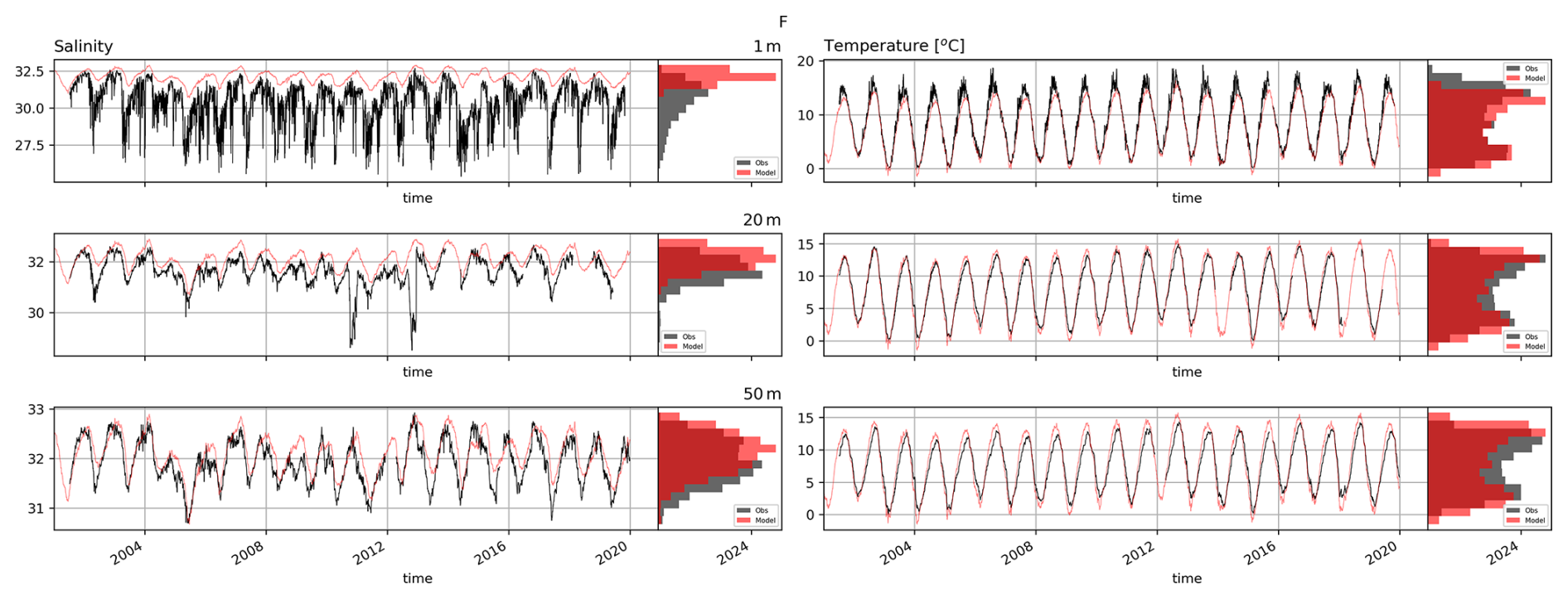
Figure A9 Time series of salinity in temperature of MOM6 (red) and NERACOOS mooring measurements (black) at buoy F.

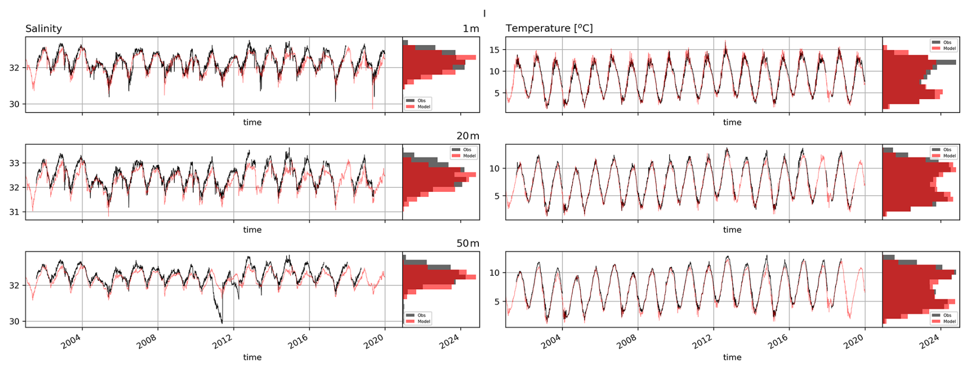
Figure A10 Time series of salinity in temperature of MOM6 (red) and NERACOOS mooring measurements (black) at buoy I.

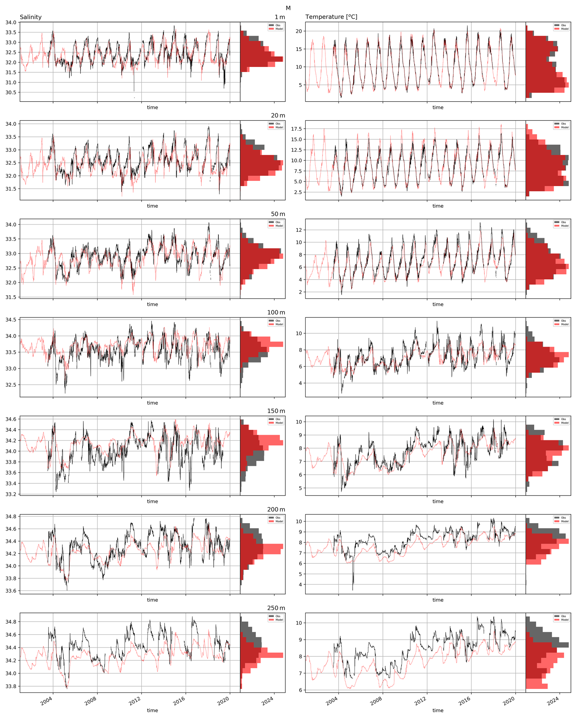
Figure A11 Time series of salinity in temperature of MOM6 (red) and NERACOOS mooring measurements (black) at buoy N.

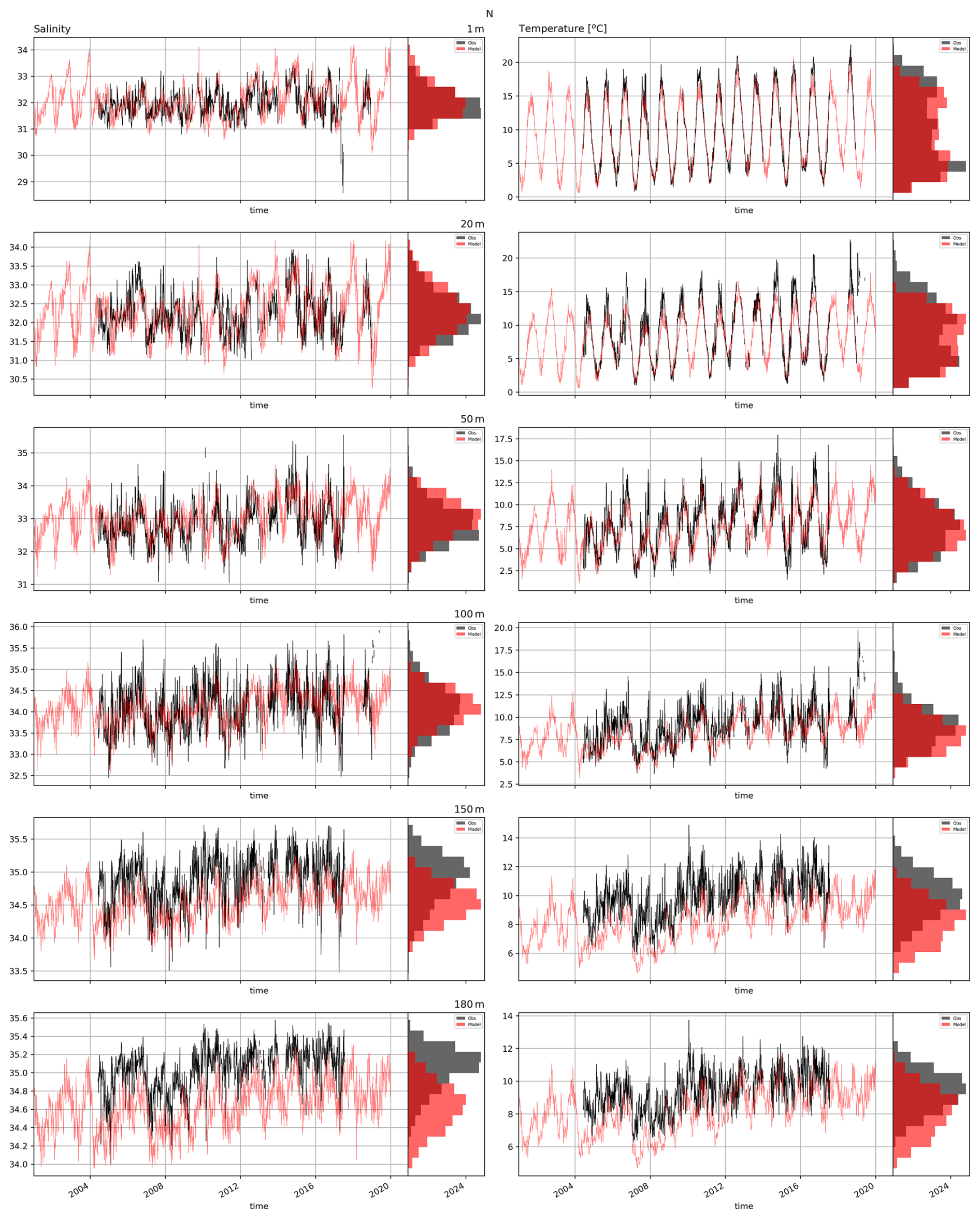
Figure A12 Time series of salinity in temperature of MOM6 (red) and NERACOOS mooring measurements (black) at buoy M.

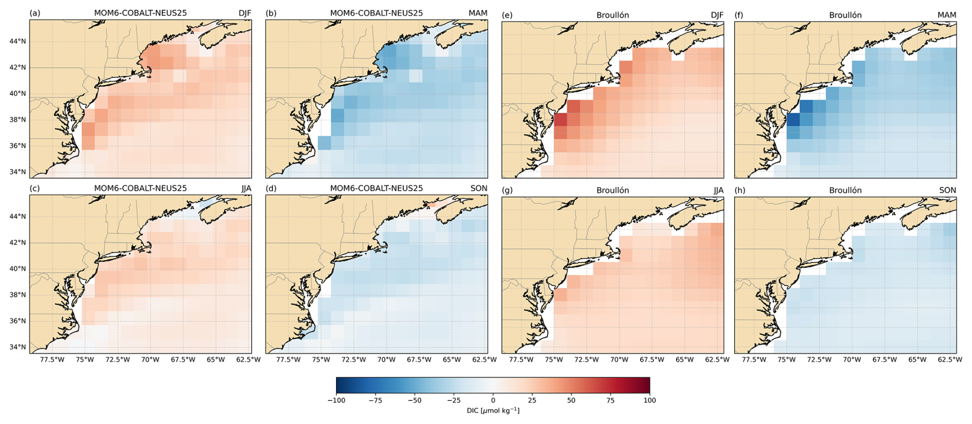
Figure A13 Seasonal climatological anomalies maps of DIC integrated over the upper 10 m considering MOM6-COBALT-NEUS25 and Broullón with respect to the total period. the number of horizontal points is shown in the label. DIC averages for MOM6-COBALT-NEUS25 and Broullòn are 2088 and 2026 µg kg⁻¹.