SNOWstorm (v1.0) – a deep-learning based model for near-surface winds and drifting snow in mountain environments

Wind-driven redistribution of snow and the resulting heterogeneous snow accumulation poses a major uncertainty in mountain hydrology and distributed glacier mass balance models as it is often neglected. High-quality information on the fine-scale wind structure is crucial to predict snow redistribution, but past approaches either relied on highly simplified assumptions or on computationally expensive numerical simulations, inhibiting the application for long-term studies.

To bridge this gap, we introduce SNOWstorm – the snow drift sublimation and transport model. It is designed as a deep-learning based emulator model, that is trained on data from high-resolution (Δx=50 m) numerical simulations in semi-idealized conditions, to be applicable for winter-time conditions in glaciated mountain regions in mid- to high latitudes. The model can be driven with input of standard atmospheric variables from coarse- to meso-scale numerical models and predicts near-surface wind fields, and rates of wind-driven snow mass change, drifting snow sublimation and snow transport. Validation experiments show that the model reproduces major terrain-induced flow features as well as patterns of snow redistribution. In a first real-world application study on a glacier in the European Alps, SNOWstorm predicts wind fields and drifting snow patterns comparable to nested numerical large-eddy simulations, though at more than five orders of magnitude less computational expense. The model thus shows the potential to be used in future studies on multi-seasonal influence of snow redistribution on glacier mass balance in various climatic settings.

1 Introduction

Snow accumulation in mountain environments can strongly differ over short distances. This heterogeneous snow accumulation can play an essential role in mountain hydrology, glacier mass balance or avalanche risk. Therefore, a representation of this variability is crucial for reliable glacier projections, run-off forecasts, weather predictions and avalanche risk assessments. The underlying processes leading to the variability in snow accumulation are classically divided into pre- and post-depositional processes (Mott et al., 2018). Pre-depositional processes include orographic precipitation enhancement, cloud-microphysical and thermodynamic interactions of snow particles with the surrounding atmosphere, as well as interaction with near-surface flow features leading to preferential deposition of snowfall (e.g., Zängl, 2007; Houze, 2012; Mott et al., 2014; Vionnet et al., 2017; Gerber et al., 2019). Post-depositional redistribution mainly takes place due to avalanches and drifting and blowing snow. This encompasses snow being eroded from the ground given strong enough wind shear, potentially getting mixed over deep layers, transported by the wind and deposited at sheltered locations (Mott et al., 2018).

These processes span a wide range of spatial scales. Erosional and depositional snow bedforms have scales of centimeters to several meters (Filhol and Sturm, 2015), and drifting snow leads to heterogeneities in snow height distribution at the scale of meters (Mott et al., 2011; Voordendag et al., 2024), while suspended snow may be transported over distances of hundreds of meters. Therefore even simulations at resolutions of five meters may not represent processes at all relevant scales (Mott and Lehning, 2010). However, major slope-scale patterns of redistribution can be captured with resolutions on the order of tens of meters (Mott and Lehning, 2010; Voordendag et al., 2024). Additionally to the mere mass redistribution effect of drifting and blowing snow, sublimation from airborne snow particles and the resulting cooling and moistening effect on the surrounding atmosphere (Groot Zwaaftink et al., 2011; Lundquist et al., 2024; Reynolds et al., 2024; Saigger et al., 2024; Sigmund et al., 2025) can have substantial influence. Apart from that, alternation of the snow surface structure due to drifting snow (Filhol and Sturm, 2015) has been shown to influence near-surface patterns of air flow and turbulent exchange, as well as subsequent snow redistribution patterns (Mott et al., 2010; Vionnet et al., 2013; Amory et al., 2017). In the past, modeling approaches to represent drifting snow have been implemented with various degrees of complexity, spanning from empirical, diagnostic and one-dimensional approaches (e.g., Liston and Sturm, 1998; Déry and Yau, 1999; Winstral and Marks, 2002; Warscher et al., 2013) to drifting snow modules integrated into numerical atmospheric models (e.g., Sauter et al., 2013; Vionnet et al., 2014; Sharma et al., 2023; Saigger et al., 2024)

In glaciological contexts, redistribution of snow by wind and avalanches has long been recognized as an important contributor to glacier mass balance (Cuffey and Paterson, 2010; Sauter et al., 2025). For example, Terleth et al. (2023) found that drifting snow contributes 18.7 % to the winter mass balance of Storglaciären, Sweden. Temme et al. (2023) could improve their surface mass balance simulations in Cordillera Darwin, Chile, when including a simple redistribution scheme. On the other hand, drifting snow sublimation has been shown to be the dominant ablation term for glaciers in Pascua Lama, Dry Andes of Chile (Gascoin et al., 2013). Locally, surface albedo and thus energy balance is highly influenced by the presence of snow on the surface (Cuffey and Paterson, 2010) and therefore can be changed by exposing or covering bare ice due to redistributed snow. Despite this importance, most recent studies with distributed energy and mass balance models neglect redistribution of snow (e.g.,  Mortezapour et al., 2020; Blau et al., 2021; Abrahim et al., 2023; Khadka et al., 2024; Noël et al., 2025; Oulkar et al., 2025). However, even when including drifting snow in mass balance calculations, lacking detail in the wind field can still cause large differences between measured and modeled snow accumulation (Lambrecht and Mayer, 2024; Temme et al., 2025).

The availability of high-resolution wind fields poses a major challenge in modeling wind-driven redistribution and snow fall heterogeneity in mountain environments. Nested large-eddy simulations (LES) were proven to successfully represent wind systems in complex terrain (e.g., Umek et al., 2021; Goger et al., 2022) and to capture the interaction with snow redistribution and precipitation mechanisms (Vionnet et al., 2017; Gerber et al., 2018, 2019; Voordendag et al., 2024). However, due to the high computational demands this approach could only be applied to short case studies over small domain sizes. To circumvent this problem for longer analysis time frames, a number of approaches were introduced to predict high-resolution wind fields at low computational cost. These include, e.g., various approaches for extrapolation of observed wind based on topographic descriptors (Winstral and Marks, 2002; Liston and Elder, 2006; Strasser et al., 2008; Schirmer et al., 2011) or wind library approaches with pre-computed wind fields from diagnostic downscaling tools like WindNinja (introduced by Wagenbrenner et al., 2016, used and adapted by Vionnet et al., 2021 and Marsh et al., 2023), or pre-computed fields from a numerical model (Dadic et al., 2010). Statistical models building on data sets of numerical simulations under idealized conditions were introduced by Helbig et al. (2017) and Helbig et al. (2024). Reynolds et al. (2023) introduced HICAR as the high-resolution version of the Intermediate Complexity Atmospheric Research model (ICAR,  Gutmann et al., 2016; Horak et al., 2021) building on linear mountain wave theory that achieves a speedup factor of 594 compared to numerical simulations with the Weather Research and Forecasting Model (WRF).

In recent years, machine learning (ML) methods have gotten large attention in the atmospheric sciences and specifically for downscaling tasks (Molina et al., 2023) due to their computational efficiency. For wind fields in mountain regions at meso-scale resolution such models have been introduced trained on operational numerical weather predictions (Miralles et al., 2022; Dupuy et al., 2023; Sekiyama et al., 2023). Dujardin and Lehning (2022) and Le Toumelin et al. (2023) developed ML-based downscaling models for near-surface wind in complex terrain at very high spatial resolution of 50 and 30 m, respectively. For this, Dujardin and Lehning (2022) trained their model on data from weather stations, meso-scale numerical weather predictions, and high-resolution digital elevation models in Switzerland. The model of Le Toumelin et al. (2023) used the data set of idealized numerical simulations across diverse synthetic topographies of Helbig et al. (2017) as training data. Despite the successful implementation, this model has the shortcomings of assuming a neutral stratification of the atmosphere, neglecting turbulent motions and applying a linear scaling with respect to the coarse-scale wind velocity.

Building on these recent developments, we present in this work a new downscaling model, that is tailored towards assessing near-surface winds and redistribution of snow in mountain environments and that addresses the shortcomings of earlier models. With our model, the snow drift sublimation and transport model (SNOWstorm), we specifically aim for these characteristics:

• coupled prediction of near-surface winds, snow mass change rate on the ground, sublimation from airborne snow particles and snow transport rate,

• large speed up rate compared to conventional numerical simulations to be feasible for multi-seasonal applications on a regional scale,

• direct applicability of the model over a wide range of regions world wide given only high-resolution terrain information and standard atmospheric input variables at large- to meso-scale resolution,

• representation of non-linear responses to changes in the atmospheric background conditions,

• explicit representation of near-surface large turbulent structures in the wind field,

• representation of interactions between drifting snow and the background atmosphere.

With these requirements in mind, we build a ML-based emulator model that is trained on a set of semi-idealized numerical simulations in LES setup which are representative for winter-time flow conditions in mountain environments. The paper is structured as follows: Sect. 2 introduces the training data set as well as the design and training of the ML model. Additionally, the approach to couple the trained model to coarse-scale atmospheric input is introduced here. The model is validated in Sect. 3. As a brief proof of concept we present in Sect. 3.3 a first real-world application of SNOWstorm in the European Alps revisiting the case study of Voordendag et al. (2024).

2 Data and Methods

2.1 Training Data

The main goal of this work is to build a model that is applicable for a wide range of atmospheric conditions and over a wide range of regions, focusing on winter-time mountain environments in mid- to high latitudes. Work by Helbig and Löwe (2012) showed that essential characteristics of real terrain like slope statistics can be represented by artificial topographies such as Gaussian Random Fields. Atmospheric simulations run on a large set of these synthetic topographies have been used to develop downscaling tools for near-surface wind, subsequently applicable for real terrain (Helbig et al., 2017; Le Toumelin et al., 2023). Building on this idea, of representing real-world characteristics in a synthetic setting, with the goal of a tool, that is applicable independent of the geographic location, we develop our training data. The focus of our approach, however, lies in capturing the harmonics in the atmosphere-terrain interaction for terrain-induced flows with large-scale forcing, as previously done for modeling approaches building on linear mountain wave theory (e.g., Smith and Barstad, 2004; Sauter, 2020). For this, the synthetic topographies used in our approach are designed to reflect the range of spectral characteristics of real terrain. In the same way, the atmospheric conditions represent the range of harmonic properties found throughout winter-time mountain regions in mid- to high latitudes.

The numerical simulations are run at very high resolutions (Δx=50 m) in LES setup to explicitly resolve large turbulent motions and to capture relevant snow redistribution at slope scales. The simulations are run with a coupled drifting snow scheme, to explicitly represent interactions between the drifting snow and the atmosphere. These numerical simulations are subsequently used as ground truth to train the ML model. The finished ML model can then be driven with input from large- to meso-scale atmospheric models and realistic topography. Due to the design of the synthetic topographies and the numerical simulations, applications of the finished ML model are fixed to the horizontal resolution of Δx=50 m used in the training data.

2.1.1 Synthetic Terrain Generation

As introduced above, the training data used for our model aims to represent the harmonics in the atmosphere-terrain interaction of terrain-induced flows with large-scale forcing. Rather than using a set of real terrain, which would be subject to potential sampling bias, we build a data set of synthetic topographies that reflect fundamental spectral characteristics found in real terrain. For this, we first analyze spectral slope characteristics of real terrain and subsequently use these characteristics to build a set of new, synthetic topographies.

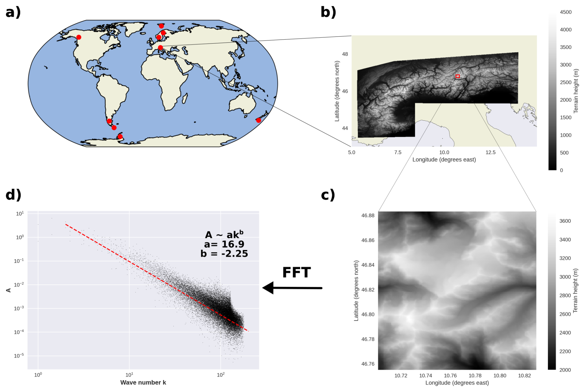
Figure 1 Overview of topographic analysis: Regions marked by red dots in (a) are analyzed, tiles of 256×256 grid points are extracted form DEMs with Δx=50 m (b–c), for each tile, a 2D-FFT is calculated, the spectrum is approximated by Eq. (1) (d).

We start by analyzing terrain for spectral slope characteristics following the same method as introduced by Young and Pielke (1983) with 2D-applications by Steyn and Ayotte (1985) and Salvador et al. (1999). We analyze the mountain regions depicted in Fig. 1a, focusing on glaciated mountain ranges in mid- to high latitudes ranging over the entire world with dominant large-scale atmospheric forcing. In a first step, 30 m resolution digital elevation models (DEMs) of the Copernicus DEM GLO-30 (European Space Agency, 2019) of the regions shown in Fig. 1a are resampled to 50 m horizontal resolution and cut to tiles of 256×256 points in order to fit the requirements in terms of domain size and resolution of the later model (Fig. 1b–c). To avoid large spectral amplitudes at wavenumber 0, the deviation from a linearly fitted plane is calculated. Additionally, a cosine filter is applied on the outermost 10 grid points at each border to taper out the terrain in order to avoid discontinuities at the tile edges. On these filtered and de-trended DEMs a 2D Fast Fourier Transform (FFT) is applied (Cooley and Tukey, 1965). We take the module of the complex values and normalize by the domain size in order to get the amplitude spectrum A. Subsequently, as indicated in Fig. 1d, the decay of spectral amplitude with increasing wavenumber k is described by the function

$$\begin{array}{}\text{(1)}& A=a{k}^b,\end{array}$$

with a and b being the intercept and slope of the power-law scaled spectrum. Here, stronger negative values of b indicate less spectral amplitude contained in smaller wave lengths and thus more smooth terrain. This procedure is applied to in total 54 022 tiles.

Figure 2 shows the distribution of spectral slope characteristics for the analyzed mountain regions. With the values resembling earlier studies for different regions (Young and Pielke, 1983; Steyn and Ayotte, 1985; Salvador et al., 1999), and values only differing slightly between the regions analyzed here (not shown), this analysis indicates the transferability of these spectral slope characteristics.

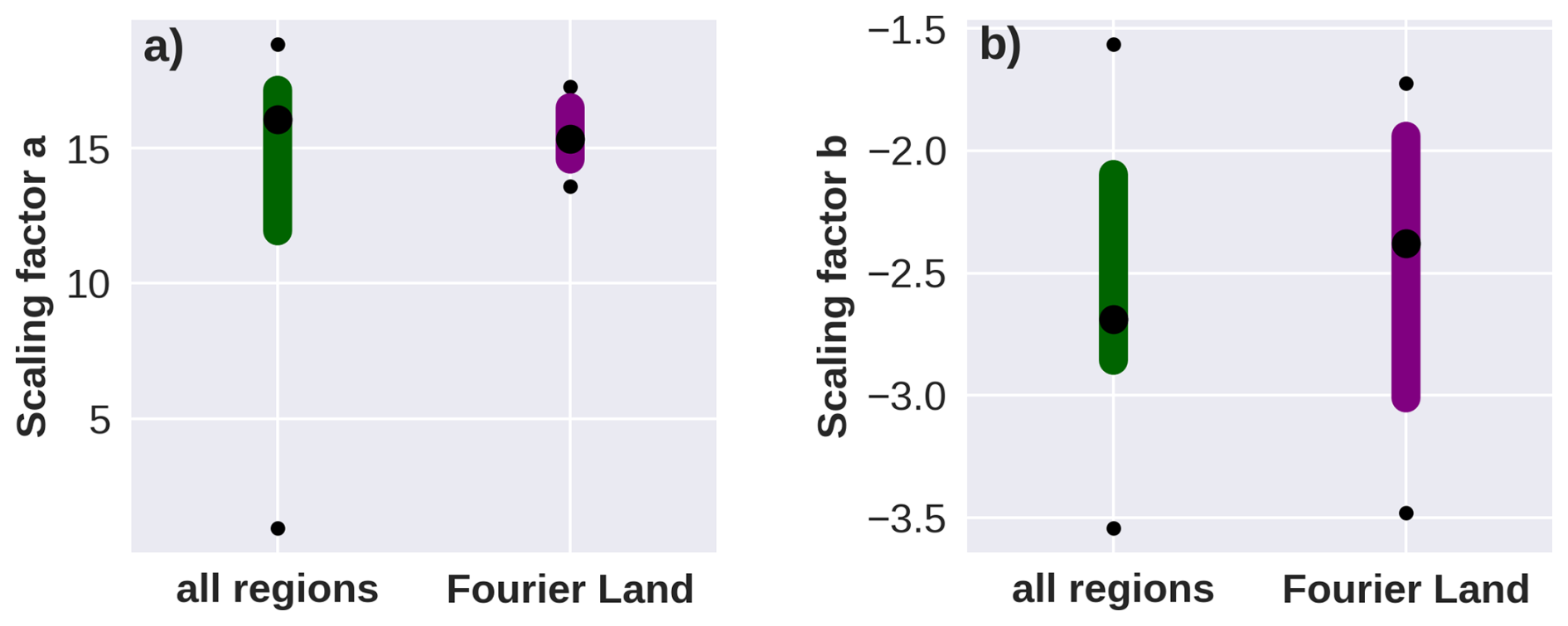
Figure 2 Distribution of factors a and b from Eq. (1) for topography tiles from selected regions (“all regions”, see Fig. 1) and synthetic topographies (“Fourier Land”). Depicted are median (large dot), 10th and 90th percentile (range of colored bar) and minimum and maximum value (small dot) of the distribution.

Our method to create new, synthetic topographies (“Fourier Land”) builds on replicating the spectral slope characteristics described above. It follows the approach shown in Jacobs et al. (2017) for artificial surfaces in material sciences, the approach of Trujillo et al. (2009) to create artificial fields of snow height distribution, and methods used to create landscapes and water surfaces in movies and computer games. On a matrix of white noise a 2D FFT is applied, the amplitude is scaled following Eq. (1). After that an inverse FFT is applied to create the topography. In total, a set of 72 topographies was created with values for a and b randomly drawn from values in the range of the ones observed in real terrain (Fig. 2). A small subset of example topographies with different spectral slope settings is shown in Fig. S1 in the Supplement. These 72 synthetic topographies are later used as terrain input for the numerical simulations. In order to avoid steep slope angles (<40°) that would cause issues with numerical stability in the simulations, we omit the smallest negative values of $b>-\mathrm{1.7}$ and very high values of a>18. Very low values of a<13 are also neglected, as these stem from tiles with almost flat topography. With this in mind, our topographies are slightly smoother than real topography and do not represent the extreme values in the variability of slope angles as well as of other commonly used terrain descriptors like topographic position index (TPI,  Weiss, 2001), maximum upwind slope angle (Winstral et al., 2002) or the terrain curvature (not shown).

2.1.2 Numerical model

In order to create the training data set, simulations with the Weather Research and Forecasting (WRF) model (Skamarock et al., 2019) are conducted. We use the Advanced Research WRF version 4.3.1 with the coupled snow drift module of Saigger et al. (2024) and online LES diagnostics WRFlux, version 1.3.2 of Göbel et al. (2022). Each model domain consists of 256×256 grid points with a horizontal grid spacing of Δx=50 m and 81 terrain-following vertical levels.

The lowest mass point is located at approximately 10 m above the ground, the model top is set to 12 000 m with Rayleigh damping activated for the upper 5000 m.

With the ideal-case setup of our simulations, only a reduced number of physical parameterizations are used. No parameterizations for radiative transfer or microphysics are employed. We use the Revised MM5 surface layer scheme (Jiménez and Dudhia, 2012) and the scale-adaptive sub-grid scale turbulent closure scheme (SMS-3DTKE) of Zhang et al. (2018) (km_opt = 5) blending between LES with the turbulence closure of Deardorff (1980) and the PBL-scheme of Nakanishi and Niino (2006) at the meso-scale limit. No land-surface parameterization is employed which also means that no explicit treatment of snow processes on the ground is in place. Instead we define a “passive” snow layer with prescribed thickness and density that only experiences wind-driven erosion or deposition. All simulations employ the drifting snow scheme of Saigger et al. (2024), in which snow erosion depends on snow density and surface shear stress. Airborne snow is transported by the resolved three-dimensional wind and parameterized turbulent mixing with a super-imposed particle subsidence. In our simulations, sublimation from drifting snow particles and its cooling and moistening effect on the ambient atmosphere is represented; the surface particle radius is set to $\mathrm{2}\times {\mathrm{10}}^{-\mathrm{4}}$ m.

In total we run 720 individual simulations with unique atmospheric conditions. For each simulation the terrain height is defined by one of the artificial topographies described above, which means that ten simulations with different atmospheric conditions are conducted on each topography. All simulations are initialized with horizontally homogeneous profiles of potential temperature, specific humidity and the meridional and zonal wind component. These profiles are calculated from values of wind speed and direction, static stability, expressed as Brunt-Väisällä Frequency, and ground-level pressure, temperature and relative humidity. The values for ground-level pressure, temperature and humidity are taken randomly from within the ranges shown in Fig. 3c–e, reflecting the variability over winter-time mountain environments. For each simulation a unique combination of wind speed and stability (ranging from neutral to isothermal conditions) is drawn. From the arrays of wind speed and stability, each possible combination is used once as initial conditions, therefore, every stability class covers the entire range of wind velocities and vice versa (Fig. 3h). Every full degree of wind direction is represented twice throughout the simulations. Note that initial profiles of wind speed, direction, stability, and relative humidity are vertically constant, neglecting, e.g., conditions with vertical wind shear or variations in stability. In order to ensure that snow is continuously present on the ground for the entire simulation period, it is initialized with a thickness of 1 m. Snow density is drawn randomly from the range of plausible values (very low-density snow to ice density) with the distribution skewed towards fresh-snow densities. The roughness length is set constant over each domain with values representing snow-covered surfaces (Fig. 3g,  Fitzpatrick et al., 2019). In our simulations, the entire domain is assumed to be uniformly snow covered, and free of vegetation.

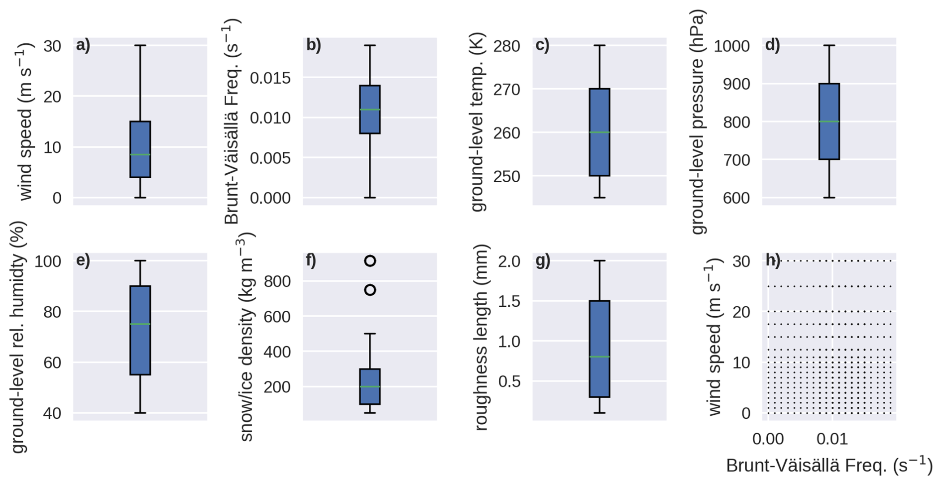
Figure 3 Distribution of the atmospheric input variables and surface conditions to drive the individual numerical simulations of the training data (a–g). The combinations of wind speed and Brunt-Väisällä Frequency used in the individual simulations are depicted in (h).

We run the simulations with a time step of 0.5 s until the near-surface turbulent fluxes have stabilized. We then use the stabilized, quasi-steady state fields with established turbulent structures and drifting snow fluxes as training data for the machine learning model. Our synthetic topographies are periodic by design, which allows us to employ periodic boundary conditions. These lead to a quick convergence of the turbulent fluxes throughout the entire domain without the need of buffer zones or perturbations at the domain boundaries (e.g., Krieger et al., 2025). Visual inspection showed that turbulent fluxes stabilized within the first three to four hours of internal model hours, in line with earlier ideal-case atmospheric simulations (e.g., Kirshbaum and Durran, 2004). Thus, all simulations were run for six hours with the first four hours disregarded as spin-up. The fields of the last two hours were averaged and accumulated, and used for later training. The averaging over two hours is used to smooth out potential un-steady fluctuations especially in weak-wind situations and in wake regions, while larger, steady-state features remain.

2.2 SNOWstorm

2.2.1 Basic design and data handling

In the past, convolutional neural networks (CNNs) have proven to successfully identify spatial structures especially in gridded data (LeCun et al., 2015). Building on that, we use the U-Net (Ronneberger et al., 2015) as the basic architecture in our study. U-Nets are fully convolutional networks that were first introduced for image segmentation, but have also been successfully applied for model emulating tasks in atmospheric sciences (e.g., Dupuy et al., 2023; Höhlein et al., 2020; Le Toumelin et al., 2023; van der Meer et al., 2023). Typically, U-Nets consist of an encoder path and a decoder path. In the encoder path, blocks of convolutional layers (in our case 3×3 convolution kernels with stride of 1 and circular padding, Fig. 4) and non-linear activation functions (in our case leakyReLU), followed by pooling layers (in our case 2×2 Max Pooling with stride of 2) are used to encode spatial patterns with increasing levels of abstraction and decrease the spatial resolution of the data. After each pooling layer, the number of feature maps is increased to compensate for the loss in spatial information. In the decoder path, blocks of up-sampling operations, followed by convolutional layers and non-linear activation functions are used to reconstruct high-resolution relationships. Additionally, skip connections are employed, where information is directly passed from the encoder path to the decoder path in order to preserve high-resolution spatial information. In total, our U-Nets consist of each four encoder and decoder blocks and a bottleneck of dimensions $\mathrm{16}\times \mathrm{16}\times \mathrm{512}$ (Fig. 4).

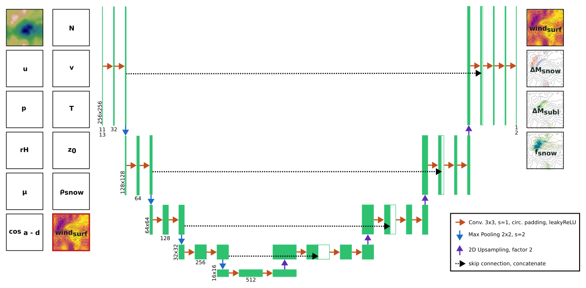
Figure 4 Schematic depiction of the U-Net architecture used for individual SNOWstorm model components. Green blocks and numbers indicate dimensions of feature maps, arrows show the individual operations. Squares on the left and right side symbolize the different input and output fields of the model (only one of the output fields for each U-Net, near-surface wind (red square) used as additional input in U-Nets for ΔM_snow, ΔM_subl, and f_snow). The output for wind_surf and f_snow has dimensions $\mathrm{2}\times \mathrm{256}\times \mathrm{256}$ as the components in x and y direction are predicted separately.

We train a separate U-Net for each of our four predictants (near-surface winds (wind_surf), snow mass change rate (ΔM_snow), vertically integrated sublimation rate (ΔM_subl), vertically integrated snow transport rate (f_snow, vertically integrated product of snow particle mass concentration and wind vector). As predictors, we use the high-resolution field of terrain height, and the low-resolution atmospheric fields and surface values (snow density ρ_snow, roughness length μ, offset elevation z₀) that the WRF simulations were driven by (Fig. 4). The atmospheric fields include meridional and zonal wind components (u, v), static stability expressed as Brunt-Väisällä Frequency (N), and surface-level values of air pressure (p), temperature (T), and relative humidity (rH). In addition to the terrain height we provide extra terrain information as a predictor similar to previous work (Dujardin and Lehning, 2022; Dupuy et al., 2023). Here we provide cos _a−d, the cosine of the difference angle between the ambient wind direction and the local slope aspect angle to indicate slopes exposed and sheltered from the ambient wind. Apart from that, the predictions of wind_surf are given as an additional predictor to the other U-Nets. This additional input and the transfer of information from the wind model to the snow-related models drastically improved the learning process of the subsequently executed models.

We perform a z-score normalization on all input and output fields. Additionally, we applied additional log-transformations for ΔM_snow and ΔM_subl as well as a square-root transformation on the terrain height and for f_snow, in order to reduce the positive skewness in the respective distributions and improve the training process of the model.

2.2.2 Training

The most important hyperparameters for the model training are summarized in Table S1 in the Supplement. For all but f_snow the mean squared error (MSE) was used as the loss function. Here, the mean absolute error (MAE) proved more successful. During model development we tested to include penalty terms in the loss function to ensure mass conservation between ΔM_snow and ΔM_subl. However, dividing into separate U-Nets for ΔM_snow and ΔM_subl and using the MSE provided better results.

We split the data set in test ($\mathrm{1}/\mathrm{8}$, 90 samples: all respective simulations over 9 randomly drawn topographies), validation ($\mathrm{1}/\mathrm{8}$) and training ($\mathrm{6}/\mathrm{8}$). With the periodic nature of our data, we are able to employ data augmentation by shifting the fields in x or y direction by a random distance (see example in Fig. S2), which much improved model robustness (Goodfellow et al., 2016). Other commonly used data augmentation techniques like rotating, flipping, linear rescaling or splitting of the data were deemed impractical for our applications. Thus, in each training epoch, the training set is once presented in unchanged form and once with each sample shifted by a random distance. The individual models are trained until convergence is reached and no indications of overfitting are present (Goodfellow et al., 2016) (Fig. S3).

2.3 Coupling with real-world atmospheric input

We provide a coupling module to run SNOWstorm with real-world atmospheric input. This extracts relevant fields from the atmospheric input data sets and brings them into a form usable for SNOWstorm. Here we provide routines for coupling to data from ERA5 and WRF, however, driving SNOWstorm with other datasets of, e.g., regional reanalyses is theoretically possible. A DEM has to be provided at a spatial resolution of 50 m. All subsequent steps are performed on the spatial grid of this DEM. To be consistent with the training data, the elevation of the lowest point in the domain is subtracted from the DEM and a square-root filter is applied, the offset elevation (z₀) is given to SNOWstorm as an additional input field. Above-crestheight wind and stability are extracted and calculated at defined pressure levels (default: 600 hPa for wind and layer between 600 and 500 hPa for stability; future users are advised to adapt this, in case model topography is intersecting with these levels). All ground-level input fields (pressure, temperature, relative humidity) are extracted at the ground level of the input atmospheric data set. Subsequently, pressure is reduced from the elevation of the input data set terrain to the offset elevation z₀ using the hydrostatic equation. Temperature is reduced with a moist-adiabatic lapse rate of Γ_m=0.0065 K m⁻¹, while relative humidity stays unchanged. All extracted and calculated fields are then interpolated bi-linearly to the grid of the fine-scale DEM. In the current version of SNOWstorm, snow density and aerodynamic roughness length have to be provided and are then constant throughout the domain. The SNOWstorm-predicted fine-scale near-surface wind field is provided as additional input for the predictions of ΔM_snow, ΔM_subl and f_snow. Before the call of SNOWstorm, all input fields are normalized with the normalization factors derived during training; output fields are back-transformed accordingly.

In the example case of Sect. 3.3 we use this coupling strategy with specifications for individual experiments as described in Sect. 3.3.2.

3 Validation of SNOWstorm

3.1 Cross validation

To provide an overview on the performance of SNOWstorm, we show examples of SNOWstorm predictions for select cases in the test data set, unseen during training, and results from cross validation experiments. We run a six-fold cross validation for all individual ML-models. Here we compute the error between the SNOWstorm-predicted fields and the corresponding WRF fields at grid-cell scale. Additionally, we divide the errors into classes of wind speed based on the WRF-predicted wind speed. Overall mean absolute errors in wind speed are around 0.8 m s⁻¹, with a bias of −0.12 m s⁻¹ and a Pearson correlation coefficient of 0.94 (Fig 5a–c). The spread over the individual cross validation experiments is low with the MAE between 0.75 and 0.87 m s⁻¹, the bias between −0.06 and −0.22 m s⁻¹, and correlation coefficient between 0.92 and 0.95. With increasing wind speed also the mean error increases up to about 1.5 m s⁻¹ for grid cells with wind speed higher than 10 m s⁻¹. For the slowest velocity class below 1 m s⁻¹ SNOWstorm overestimates the wind speed by 0.16 m s⁻¹, while for all other velocity classes we observe a negative bias. This indicates that the wind fields predicted by SNOWstorm are slightly too smooth and the full range of velocity can not be represented. Pattern correlation for the individual velocity classes decreases to values around 0.7 and to 0.35 for grid cells with WRF wind speeds below 1 m s⁻¹ (Fig. 5c). Compared to the high correlation over the entire velocity range this indicates that the overall velocity distribution is captured, while local details in the wind field might be missing. As will be seen in the example cases below, SNOWstorm especially struggles to capture the flow structure in weak-wind wake regions, which is reflected in the low correlation in the lowest velocity class. Although the averaging over two hours of the training data aims to smooth the wind fields in these regions, in our experience, these situations still exhibit a less clear alignment of the flow with the local topography and the ambient wind direction, and thus cause these lower correlations. With increasing wind speeds the spread between the individual experiments increases in all error measures. This might point to a comparatively small sample size and a dependence of the performance on only a few cases.

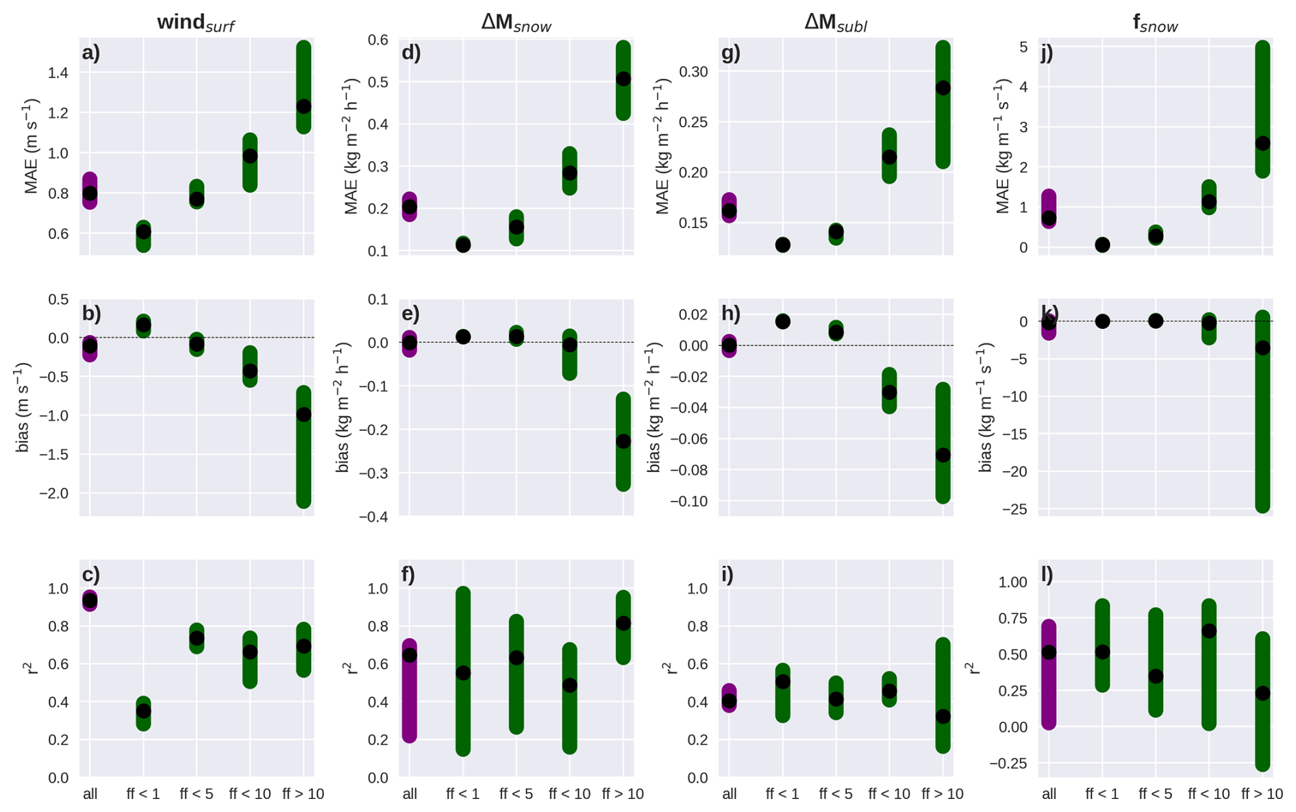
Figure 5 Grid-cell wise mean absolute error (MAE), bias, and squared Pearson correlation coefficient (r²) for cross validation experiments. Errors are depicted for wind speed (a–c), snow mass change rate (d–f), sublimation rate (g–i) and integrated snow transport (j–l to be done). Black dots and colored bars denote the median and range over the cross validation experiments. Purple bars show results for all points, green bars for points in classes of wind speed as indicated on the x axis (wind speed (ff) < 1 m s⁻¹, 1 m s⁻¹ < ff < 5 m s⁻¹, etc.). Black dashed lines in (b), (e), (h), and (k) indicate the bias of 0.

Although a direct transferability is limited, the uncertainties reported here are in a comparable range as the ones found for other ML-based models for high-resolution winds in complex terrain. Dujardin and Lehning (2022) find for their model (trained on weather station data, high-resolution terrain descriptors, and meso-scale numerical weather model output) an MAE of 1 to 1.5 m s⁻¹ with a negative bias between −0.16 and −0.04 m s⁻¹, depending on surrounding terrain characteristics. Correlation coefficients here range between 0.42 and 0.66. Le Toumelin et al. (2023) report for their ML model (trained on simulated data over synthetic topographies) a bias below 0.01 m s⁻¹, and a correlation coefficient of 0.96 in their cross validation experiments, though with a markedly lower MAE of 0.16 m s⁻¹. While being in a similar range, all these comparisons have to be made with caution, given the differences in validation strategies and the different nature and degree of complexity in the respective model setup and training data.

Errors for the predicted rates of snow mass change, sublimation, and snow transport show a similar behavior as the errors of the wind field. Overall MAE for ΔM_snow is at 0.2 kg m⁻² h⁻¹ increasing from about 0.11 kg m⁻² h⁻¹ in the lowest velocity class to about 0.5 kg m⁻² h⁻¹ for grid cells with highest wind speeds (Fig. 5d). MAE for the sublimation rate are in a similar range with 0.16 kg m⁻² h⁻¹ for all grid cells and increasing from 0.12 to 0.28 kg m⁻² h⁻¹ in the highest velocity class. Similarly, MAE for f_snow increases from 0.06 to 2.59 kg m⁻¹ s⁻¹ in the highest velocity class with 0.73 kg m⁻¹ s⁻¹ overall. Similar to the wind velocity, ΔM_snow, ΔM_subl, and f_snow are slightly overestimated in the low velocity classes and underestimated for cells with increasing wind speed. The overall bias is close to zero (ΔM_snow: $-{\mathrm{10}}^{-\mathrm{3}}$ kg m⁻² h⁻¹, ΔM_subl: $-{\mathrm{10}}^{-\mathrm{4}}$ kg m⁻² h⁻¹, f_snow: 0.17 kg m⁻¹ s⁻¹). Correlation is generally lower compared to the predictions of wind speed and with a large spread over the experiments with again possible problems with too small sample sizes (Fig. 5f, i, l).

3.2 Performance on example data sets

The following three example cases are selected to represent different atmospheric conditions that SNOWstrom is trained for and showcase the performance on different flow situations. Two cases have relatively high wind speeds and thus considerable amounts of snow redistribution (case A: Fig. 6, case B: Fig. 7), while the third one only experiences very low wind speeds and consequently no drifting snow is present (case C: Fig. S4). With the ambient relative humidity well below saturation (70 %) in case A, sublimation from drifting snow particles plays a crucial role here, while high relative humidity in case B suppresses sublimation.

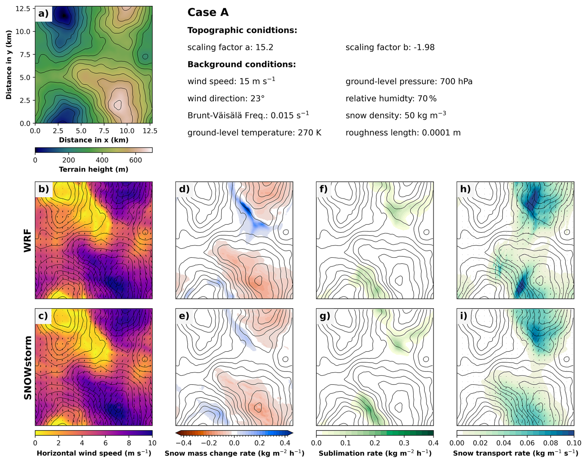
Figure 6 Example case A of SNOWstorm predictions (lower row) and WRF ground truth (middle row). Depicted are model terrain height (a), 10 m flow field (b–c), snow mass change rate (d–e), drifting snow sublimation rate (f–g) and integrated snow transport rate (h–i, arrows and colors). Model terrain height is additionally indicated by black contour lines with an interval of 100 m. Background conditions for each case are specified in the upper row. The case is part of the test data set, unseen during training.

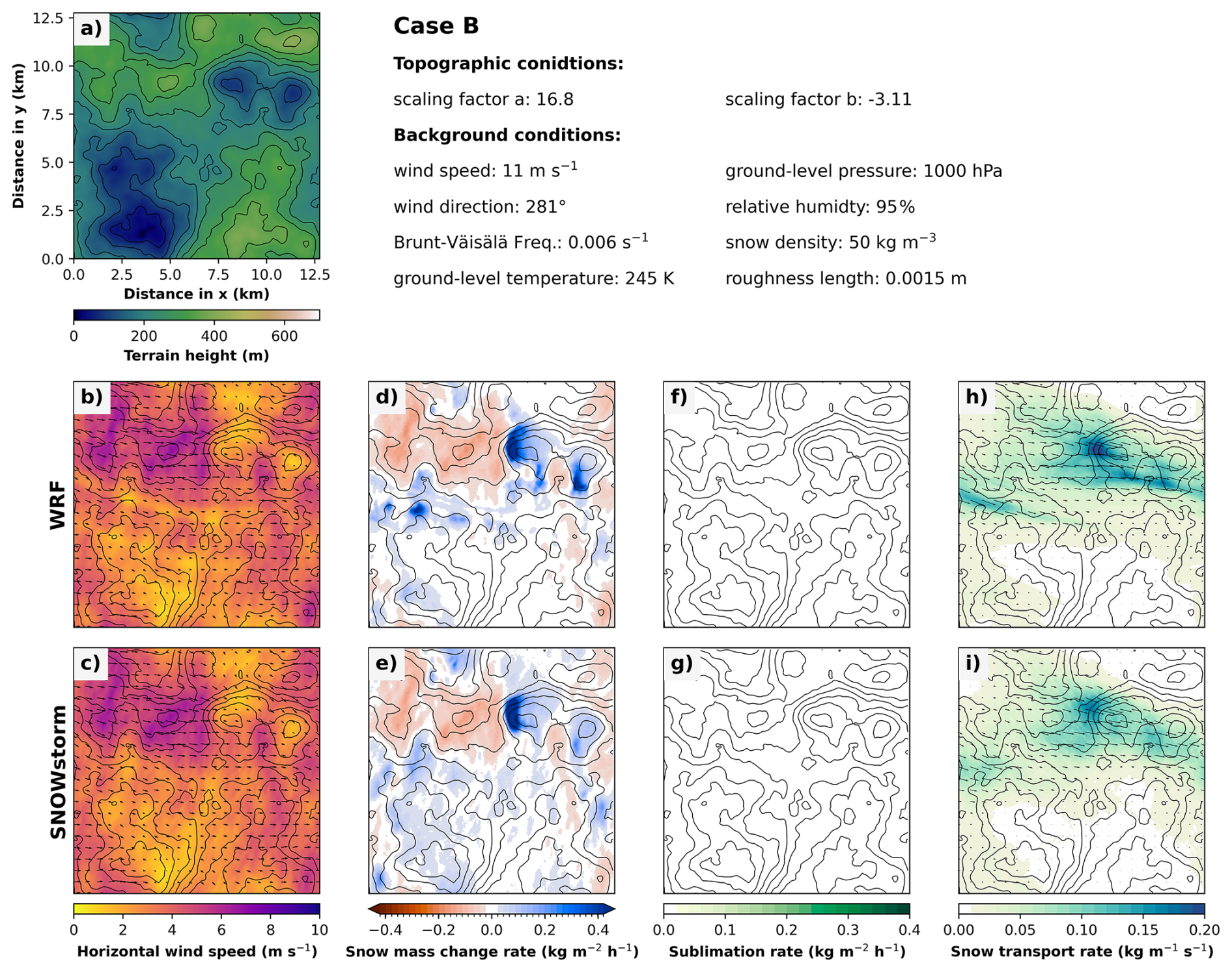
Figure 7 Similar to Fig. 6, but for case B. Note the changed colorscale for terrain height and integrated snow transport rate.

The wind fields predicted by SNOWstorm in general agree with the WRF-simulated flow fields. SNOWstorm captures the overall wind direction and speed as well as terrain-induced flow features such as acceleration at ridges, and deflection and channeling around summits, and through gaps and valleys (Figs. 6, 7, S4b–c). While capturing the general patterns in regions of lee-side flow separation (case A and C), SNOWstorm can not fully reproduce the associated sharp gradients in wind velocity as well as flow patterns in the weak-wind wake regions.

Similar to the wind fields, patterns in snow erosion and deposition generally agree with the WRF simulations. The placement of zones of erosion and deposition as well as the overall amounts in these zones fit well in cases A and B (Figs. 6, 7d–e). However, the maximum amounts of snow deposition (e.g., in the lee of the northern hill in case A, secondary patches in case B) are underestimated by SNOWstorm. In the weak-wind case C, SNOWstorm successfully predicts very low snow mass change rates below our threshold of depiction in the figure (Fig. S4d–e). However, due to its design, SNOWstorm does not recognize zero as a special value, and thus, will not necessarily predict values of exactly zero but small values close to zero in situations where no snow redistribution should occur. Over long integration time scales these small errors might become significant, so future users should consider applying zero filters for very small values. This is also true for situations of no relevant drifting snow sublimation (case B, C, Figs. 7, S4f–g): SNOWstorm successfully predicts values very close to zero, though not exactly zero. In the case A with sublimation playing an important role, SNOWstorm manages to predict the basic placement and amount of drifting snow sublimation (Fig. 6f–g). Predictions of the snow transport rate are in line with the results of the other model components: the overall shape and amounts are captured by SNOWstorm, while the zones of maximum snow transport are slightly underestimated and slightly misplaced.

In summary, wind fields predicted by SNOWstorm generally agree with the LES ground truth, except for highly turbulent flow features such as lee-side flow separations and in wake regions. Predictions of snow redistribution and sublimation as well fit to the WRF simulations. Mismatches in the simulated flow field can influence predictions of snow-related fields.

3.3 Case study: application of SNOWstorm

3.3.1 Case study overview

To provide an outlook on potential applications of SNOWstorm, we revisit the case study of 8 February 2021 on Hintereisferner, a glacier in the Austrian Alps, studied in detail by Voordendag et al. (2024), of which the main results are summarized in the following. Figure 8 provides an overview of the region and the locations of available weather stations. The event was characterized by a cold front passage during the night with fresh snowfall and a subsequent increase in wind speed and shift in wind direction, leading to large amounts of snow redistribution in the second half of the day. The amounts of snowfall and redistribution were observed by three terrestrial laser scans (TLS). The laser scanner is installed at the same location on the ridge above the glacier as the station IHE. Additionally, nested large-eddy simulations at Δx=48 m in WRF (HEF-LES) with the coupled snow drift scheme of Saigger et al. (2024) were performed. Validation of wind speeds and direction against three automated weather stations (Fig. 8 for location) showed a high accuracy of the simulated flow field. Comparison to the TLS-observed snow height change revealed that the overall amounts of snow redistribution are underestimated by the HEF-LES by about 9 %. Slope-scale patterns of snow redistribution like the position of maximum erosion on summits and exposed ridges are captured well in the HEF-LES, while smaller-scale patterns such as dune formations and interaction with sub-grid scale topography are not represented. As the TLS signal is comprised of snow redistribution, compaction and avalanching, and is limited in its scanning geometry, we will not use the TLS for direct comparison with SNOWstorm, but assume the HEF-LES to be validated against the TLS, and use the HEF-LES for validation of SNOWstorm. For more details in the methods and results we refer to the original publication of Voordendag et al. (2024).

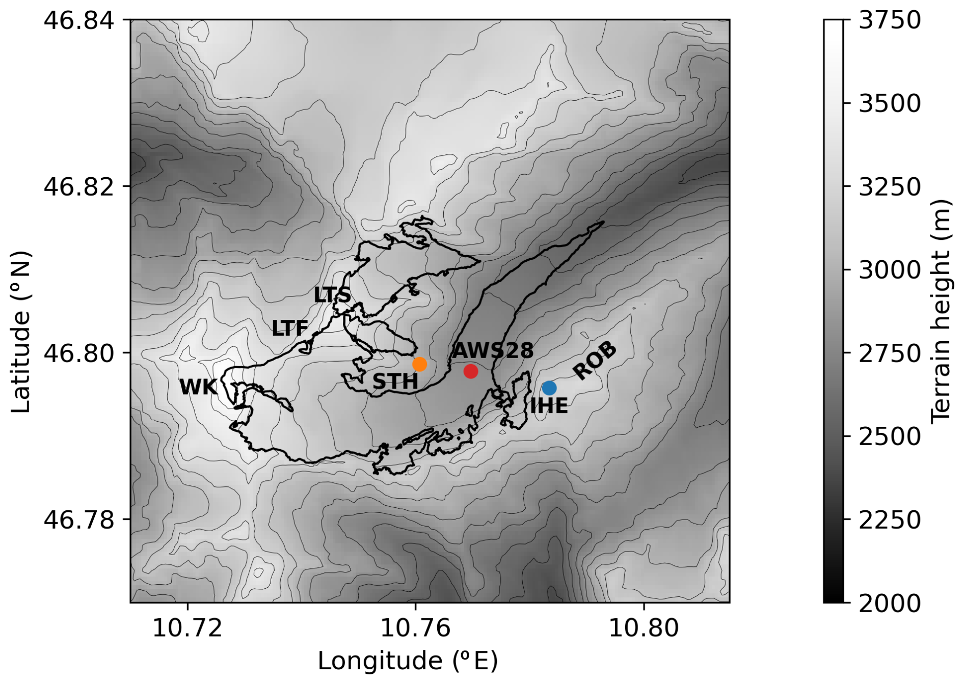
Figure 8 Overview map of Hintereisferner. Depicted are terrain height as contour colors and black contour lines (line spacing 100 m), the outlines of Hintereisferner glacier as tick black lines, and the location of weather stations as colored dots (Im Hinteren Eis (IHE), Station Hintereis (STH), temporary station on the glacier (AWS28)). Important landmarks are indicated by their abbreviations (Weißkugel (WK), Rofenberg (ROB), Langtauferer Ferner glacier (LTF), Langtauferer Spitze (LTS)).

3.3.2 Experiment setup

To better understand the behavior of SNOWstorm in real-world applications, experiments with different coupling strategies as described below and summarized in Table 1 are run and validated against the results of the HEF-LES as well as against the observations from the weather stations. The coupling to the atmospheric input is done following the procedure described in Sect. 2.3. To explore the influence of meso-scale atmospheric information, we perform experiments driving SNOWstorm with input taken from ERA5 (experiments S_ERA_∗) and the two outer domains of the WRF simulations of Voordendag et al. (2024) D01 (Δx=6 km, experiments S_WD1_∗) and D02 (Δx=1.2 km, experiments S_WD2_∗). Additionally, we run experiments with the smoothed digital elevation model used in the HEF-LES (experiments S_∗_W), and with the un-smoothed DEM of GLO-30 (experiments S_∗_G), resampled to Δx=50 m (see Table 1 for overview of experiment settings).

Table 1 Summary of input data for the different real-case experiments presented. Each experiment abbreviation consists of the model used (SNOWstorm: S), the atmospheric input data (ERA5: ERA, WRF D01: WD1, WRF D02: WD2) and the topographic input data (GLO-30: G, smoothed HEF-LES topography: W).

For the experiments we do not couple SNOWstorm to any snow model but prescribe a snow density (200 kg m⁻¹) and roughness length (0.1 mm) consistent with the ones in the HEF-LES and representative for the fresh-snow conditions on the day of the case study. Given the short duration of the case study, we consider this reasonable. However, for future long-term investigations, coupling to a snow model will be necessary.

3.3.3 Case study results

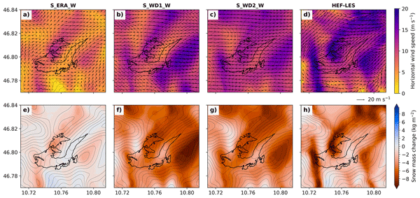
We will first focus on the second half of the day (after 14:00 UTC), the phase with highest wind speeds and snow redistribution taking place. Here, the flow fields predicted by SNOWstorm driven with input from the two meso-scale domains (S_WD1_W and S_WD2_W, Table 1) overall agree with the HEF-LES (Figs. 9b–d, 10). General flow features, such as the flow deflection and splitting on the windward side of Weißkugel summit (see Fig. 8), the deflection on the ridge north of the glacier, as well as the acceleration of the flow in summit and ridge regions, are represented in the SNOWstorm predictions (Fig. 9b–d). The channeling effect in the valley is underrepresented by SNOWstorm, leading to a too strong westerly component here (Fig. 9b–d), which is also evident in the comparison to the two observation sites of Station Hintereis (STH, Fig. 10b) and the temporary station on the glacier (AWS28, Fig. 10f). With the ridgeline of Rofenberg south of the glacier (see Fig. 8) being aligned almost parallel to the ambient westerly flow, both the HEF-LES and SNOWstorm fail to reproduce the local flow field here. HEF-LES and SNOWstorm simulate a south-westerly and westerly flow on this ridge, and thus fail to reproduce the southerly flow and therefore the main direction of overflow (Figs. 9b–d, 10d).

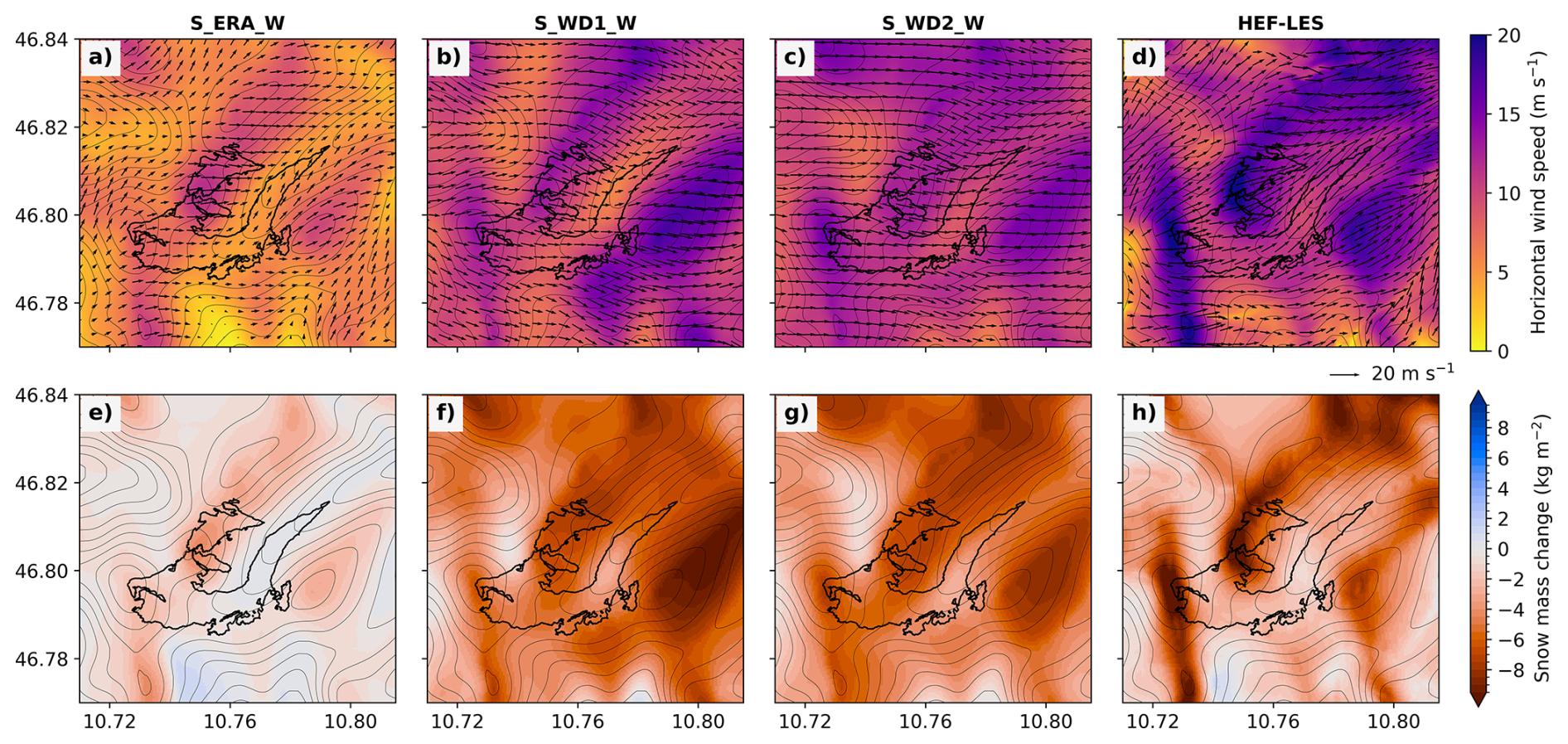
Figure 9 10 m wind field (a–d) at 8 February 2021 21:00 UTC and snow mass change due to drifting snow accumulated over the entire day (e–h) for SNOWstorm driven with various input datasets and HEF-LES. Arrows in (a)–(d) depict the horizontal wind vector, model topography is shown by black contour lines with spacing of 100 m, outlines of Hintereisferner by thick black lines.

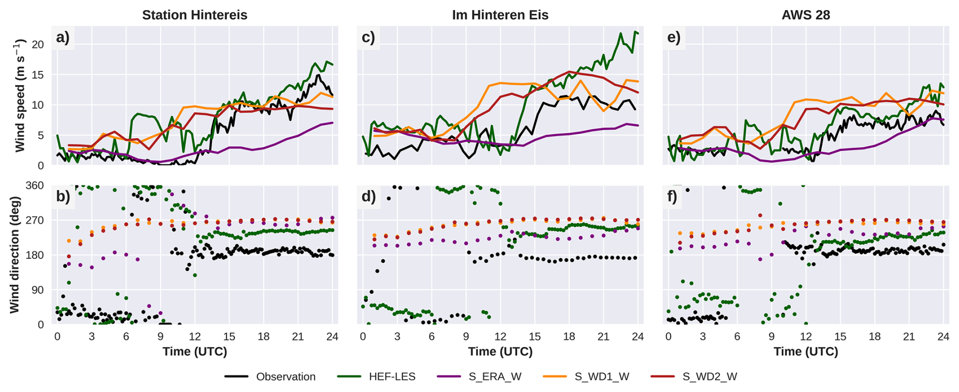
Figure 10 Time series for 8 February 2021 of wind speed and direction from observations at weather stations and model output of HEF-LES and SNOWstorm with input described in Table 1 at the corresponding closest grid point.

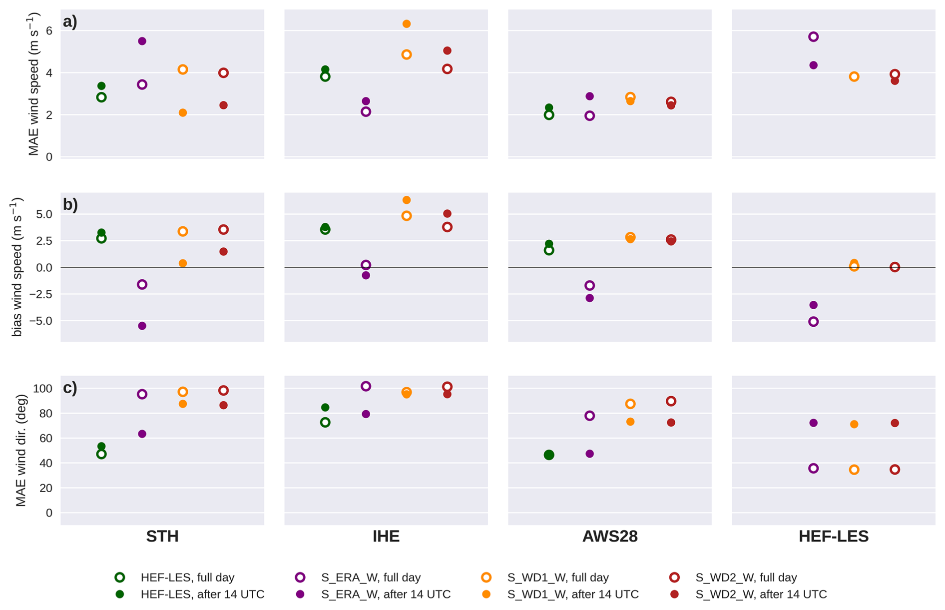
Figure 11 Error statistics for SNOWstorm experiments and HEF-LES validated against automated weather stations and point-wise against HEF-LES.

Predicted wind velocities at the three observation sites generally agree with measured overall velocities, though with absolute errors between 1.6–4.4 m s⁻¹ and a mean overestimation of 3–4 m s⁻¹ at the stations IHE and AWS28, while errors at STH are generally lower (Fig. 11a–b). Pointwise comparison to the HEF-LES shows an MAE of about 3.9 m s⁻¹, with negligible bias, however, localized velocity maxima in summit and ridge regions are underestimated by SNOWstorm (Fig. 9b–d). Errors in wind direction are in line with the aforementioned underestimation of the valley channeling and the misprediction of the local flow field around IHE described above and are in the range of 70 to 100° (Fig. 11c). These errors are higher than the overall errors seen in the cross validation experiments (Sect. 3.1) and for other comparable modeling approaches: in real-world settings, Le Toumelin et al. (2023) report an MAE in wind speed of 1.1 to 1.4 m s⁻¹, a bias of −0.17 to −0.24 m s⁻¹, and an MAE in wind direction of 14 to 57°. Dujardin and Lehning (2022) find for wind speed an MAE of 1.0 to 1.5 m s⁻¹, and a bias of −0.04 to −0.16 m s⁻¹, as well as an MAE in wind direction of 32 to 58°. Keeping in mind the short duration of the case study and the resulting limited transferability, these errors have to be viewed in context. Observed and simulated velocities have not been corrected for the height difference between the model output of HEF-LES and SNOWstorm (10 m a.g.l.) and the measurement heights (STH: 3.3 m, IHE: 3 m, AWS28: 2 m). Correcting the predicted velocities to the height difference under the assumption of a neutral stratification reduces the errors to an MAE of 1.7 to 3.9 m s⁻¹ and a bias of −0.6 to 3.7 m s⁻¹ (Fig. S5). However, with lacking information on the near-surface stratification and slightly changing surface conditions throughout the day, these height corrections can only be viewed as an estimate. While unsurprising and in line with Le Toumelin et al. (2023), that errors in the real-world application are larger than in the semi-idealized testing environment, absolute errors in the more comparable, higher velocity classes (wind speed higher 10 m s⁻¹) in the cross validation experiments are between 1.1 and 1.5 m s⁻¹ (Fig. 5a), thus closer to the errors found in the real-world experiment here. Errors of the HEF-LES benchmark to the observations are in a similar range as for SNOWstorm, providing an estimate of the overall predictability of this event. This also indicates a possible error due to an underrepresentation of microtopography, resulting in an underestimation of turbulence which is relatively common for numerical simulations in complex terrain and might have been inherited by the ML model. Errors of the coarse-scale input wind interpolated to the observation sites are in a similar range or even slightly lower than the SNOWstorm predictions and HEF-LES (see Table S2), though with the missing additional information on local flow features.

While SNOWstorm predictions in S_WD1_W and S_WD2_W show comparable results, the experiments with ERA5 input (S_ERA_W) capture the overall flow structure, though with generally too weak winds (Figs. 9a, 10, 11). This indicates that the meso-scale flow accelerations, which is lacking in ERA5, is necessary for SNOWstorm to capture the strength of the local flow field. As S_WD1_W and S_WD2_W only differ slightly, the meso-scale flow structure seems to be already represented enough in the WRF D01, and no additional information is provided by the finer input data. Nevertheless, at specific locations with large positive bias in S_WD1_W and S_WD2_W (IHE and AWS28), S_ERA_W outperforms the experiments with meso-scale input (Fig. 11). The experiments with SNOWstorm driven on the un-smoothed GLO-30 topography show similar structures (Fig. S6) and comparable errors (Table S3), which is remarkable, as the steepest slope angles here exceed all slope angles seen during training. With the finer structure in this topography also finer features in the wind field, e.g., around secondary ridge lines can be simulated.

In the first half of the day, SNOWstorm fails to capture the weak northerly flow caused by shallow cold-air inflow and overspill after the frontal passage (see Fig. S7). During the transition phase around 12:00 UTC SNOWstorm predicts the increase in wind speed about three hours too early (Fig. 10) which consequently causes a too early onset of snow redistribution and increased errors when considering the full day (Fig. 11). Both effects are explainable as SNOWstorm has the assumption that the local wind field adapts instantaneously to changes in the large-scale forcing and effects of shallow cold air advection and cold air pools have not been seen in training.

Consistent with the wind predictions, accumulated snow mass changes simulated by SNOWstorm with meso-scale input (S_WD1_W and S_ WD2_W) overall agree with the ones in the HEF-LES (Fig. 9f–h). Maximum snow erosion is predicted at the summit region of Weißkugel, and at the ridges north-west and south-east of Hintereisferner. Regions of maximum erosion are slightly more localized with higher amounts in the HEF-LES, consistent with the underestimation of maximum wind velocities in the summit regions by SNOWstorm. For example, the snow erosion in the summit region of Weißkugel is underestimated by roughly 4 kg m⁻² in SNOWstorm with meso-scale input. Apart from that, erosion zones are shifted from the ridge more towards the lee-side slopes at several places (Langtauferer Spitze, Rofenberg, see Fig. 8 for location). Due to the high overall wind speeds only very few regions of snow deposition are simulated in the HEF-LES as well as by SNOWstorm. These include especially the upper part of Langtauferer Ferner and the area around AWS28 at several instances in time in phases of stronger lee-side deceleration. The deposition zone in the lee of Rofenberg simulated in HEF-LES is not captured by SNOWstorm due to the high wind velocities here. Consistent with the too low wind velocities, SNOWstorm simulates a much smaller change in snow mass in the experiment with ERA5 input (S_ERA_W, Fig. 9e). Pointwise validation against the HEF-LES shows an MAE between 2.3 and 2.8 kg m⁻² and a correlation coefficient between 0.4 and 0.6 for the different experiments. As already seen for the wind field, the experiments with GLO-30 topography show similar results, though with smaller-scale features captured by the more detailed input topography (Fig. S6). Sublimation from drifting snow particles plays a negligible role in both modeling approaches (Fig. S8). Similar to the other variables, the overall amounts and the placement of sublimation zones predicted by SNOWstorm generally agree with the ones simulated in HEF-LES.

In summary, SNOWstorm manages to capture the general shape and strength of the flow field as well as the overall amounts and location of snow redistribution during this case study. Local details in the flow field and transition periods in the large-scale forcing remain challenging for SNOWstorm. The large advantage of the ML model, however, lies in its computational efficiency: the computations for the HEF-LES of Voordendag et al. (2024) required about 10⁴ core hours. In contrast, the predictions with SNOWstorm can be run on a single CPU in 4 s for the entire day with ERA-5 input and 0.1 and 0.3 h, respectively, with WRF input due to the longer processing time during input data preparation. This means a speedup factor on the order of 10⁵ to 10⁷ and reasonable computational demands for simulations over entire accumulation seasons.

3.4 Summary and Limitations

We tested SNOWstorm in a cross-validation experiment, on three example predictions in the semi-idealized training and testing environment, and in a short (24 h) real-world case study. SNOWstorm generally captures the overall flow situation and terrain-induced flow modifications. Uncertainties in the semi-idealized environment in wind speed are on average at 0.8 m s⁻¹, increasing with increasing background wind. In the real-world case study, the absolute error increases to 1.6 to 4 m s⁻¹, which likely stems in part from a positive bias, due to height differences of model output and observations, and in part from the more complex atmospheric and topographic settings, and possibly an underrepresentation of microtopography and inherited biases from the numerical model. These model uncertainties can be compared with errors in other ML-models for wind in complex terrain at the decameter scale like Dujardin and Lehning (2022) or Le Toumelin et al. (2023). Errors in Le Toumelin et al. (2023) are lower than for SNOWstorm both in the idealized training and testing environment (MAE: 0.16 m s⁻¹), and in real-world settings (MAE 1.1 to 1.4 m s⁻¹). Absolute errors in Dujardin and Lehning (2022) are in a comparable range (MAE: 1.0 to 1.5 m s⁻¹), though with a smaller bias in the real-world setting. However, with the short duration of the case study, and the differences in validation strategy and overall settings between the models, transferability between these reported uncertainties is limited, opening the possibility for a coordinated model intercomparison experiment.

As with any statistical model, future users of SNOWstorm are advised to be cautious when applying the model outside the range of the training data. Due to the design of the training data, this implies several limitations of the model:

• To ensure numerical stability, steep slope angles (>40°) had to be avoided in the training data. Although the case study results show consistent results even for slope angles outside the training range, future users should be cautious in cases of large steep slopes or near-vertical faces present in the domain.

• The domains in the training data are designed fully snow-covered and free of vegetation, representative for high-alpine winter-time environments. Vegetated areas can therefore not be appropriately simulated by SNOWstorm.

• The model is trained for winter-time atmospheric conditions in mid- to high latitudes and assumes an instantaneous adaption of the local flow field to changes in the large-scale forcing. Thermally-driven flow situations like local convection, katabatic flows, slope and valley wind circulations, or interactions with cold-air pools, are not represented and can therefore not be appropriately simulated by SNOWstorm.

• In its design, the output of SNOWstorm is fixed to tiles of 256×256 grid points with a horizontal resolution of Δx=50 m. For larger domian sizes, several SNOWstorm output tiles have to be produced and overlayed; a transfer to other horizontal resolutions is not possible.

4 Conclusions and Outlook

In this work we introduced SNOWstorm as a new, deep-learning based emulator model for near-surface winds and snow redistribution in mountainous terrain at high spatial resolutions (Δx=50 m). The model has a U-Net architecture and is trained on output of semi-idealized numerical simulations with synthetic topographies and atmospheric conditions representative for glaciated mountain regions in mid- to high latitudes during winter time.

We performed validation experiments in the semi-idealized testing environment and applied the model to a short case study on a glacier in the European Alps, including a comparison to both observations and nested Large-Eddy simulations (HEF-LES).

Key findings from the validation experiments in the testing environment are:

• SNOWstorm in general successfully predicts the overall spatial distribution and strength of the flow field with terrain-induced flow modifications. Position and amounts of zones of snow erosion, deposition, sublimation, and snow transport agree with the ground truth of the numerical simulations.

• Overall absolute errors in the cross validation experiments are about 0.8 m s⁻¹ with a bias of −0.12 m s⁻¹, and increase with stronger background wind speeds. The predicted wind fields tend to be smoother than the ground truth, especially in regions of sharp gradients like zones of flow separation, or in unsteady wake regions.

Key findings form the real-world application case study are:

• SNOWstorm overall succeeds to capture the general flow structure and redistribution patterns in this case study. Features like the acceleration and deflection of the flow in summit and ridge regions are reflected by the SNOWstorm predictions, while the channeling effect inside the valley is underpredicted. The general placement of zones of snow erosion and deposition agree between SNOWstorm and HEF-LES; mismatches, like an underestimation of snow erosion in summit and ridge regions are in agreement with an underestimation of wind speed here.

• Validation against automated weather stations shows absolute errors in wind speed between 1.6 and 4 m s⁻¹, notably higher than in the cross validation experiments. These higher values are possibly due to the more complex flow situation, inherited biases from the numerical model, and a height difference between model output and observation height.

• Both experiments with meso-scale input (Δx=6 km and Δx=1.2 km) show similar results, while the experiments with ERA5 input underestimate wind speeds and redistribution amounts, possibly due to the lack of information of the meso-scale flow structure.

• Experiments with the smoothed topography input from the HEF-LES and with an un-smoothed high-resolution DEM show similar results, even though slope angles in the un-smoothed case exceed slope angles seen during model training.

• One limitation of the model are localized effects of shallow cold-air advection and delayed local responses during transition phases in the large-scale forcing which are not captured well by SNOWstorm as such effects have not been seen during training.

With the very large computational speedup of more than five orders of magnitude compared to physics-based LES at Δx=50 m, the model has large potential to be used in (multi-) seasonal assessments of snow redistribution. For this, next steps will involve coupling SNOWstorm to glacier mass balance models like, e.g., COSIPY (Sauter et al., 2020) and adding routines for application over larger areas. Given the world-wide availability of high-resolution DEMs (e.g.,  European Space Agency, 2019) and the dependence on only a few standard atmospheric variables at meso-scale resolutions, recently published regional downscaling datasets in, e.g., Europe (Copernicus Climate Change Service, 2022), the Alps (MeteoSwiss, 2025), South America (Dominguez et al., 2024), New Zealand (Kropač et al., 2024) or in arctic regions (Turton et al., 2020; Copernicus Climate Change Service, 2021) can provide possible input data sets for SNOWstorm applications. Apart from that, our results show the potential of generalization of emulator models trained under semi-idealized conditions given a carefully created training data set. Similar approaches could be possible, e.g., for thermally driven flows or turbulent exchange of energy, mass and momentum in complex terrain.