The next generation sea-ice model neXtSIM, version 2

Sea ice is a key component of the climate system, and sea-ice models are required to realistically simulate climate, ocean, or atmosphere in general circulation models at high latitudes. In this paper, we present the latest version of the next-generation sea-ice model, neXtSIM, which has been developed with a particular focus on ice dynamics and motion. While many large-scale sea ice models can represent regional-to-global sea ice evolution, their representation of sea ice dynamics varies little across models, as they all use a very similar representation of the ice's internal stresses. While this works reasonably well for several quantities (e.g. sea ice volume), it fails to capture sea ice deformation features and the resulting localised changes in thickness and concentration, which likely play an essential role in ice–atmosphere–ocean interactions. The neXtSIM model has been at the core of efforts by its developers and users to explore new modelling approaches to address this shortcoming. Here, we document neXtSIM, now in version 2 of its development, to foster its use for the sea ice community and release a public version of the model. We describe the sea ice dynamics and the core of the model in detail, and discuss parameters specific to the brittle rheologies included in neXtSIM. We also document the model's specificity arising from its Lagrangian framework and its implications for coupling with other components of Earth system models. We hope that the insights provided in this study and the public release of the model will trigger innovative research in the sea ice modelling community.

1 Introduction

Sea ice is a key component of the climate system, and sea-ice dynamics play a significant role in shaping the sea-ice cover in both hemispheres; therefore, geophysical models must capture these characteristics. These dynamics are strongly influenced by the choice of sea ice rheology, and most models use a rheology based on the viscous-plastic (VP) framework suggested by Hibler (1979), which has demonstrated its ability to capture large-scale ice properties (such as area and volume) with reasonable accuracy over the years. However, it generally fails to capture localised deformations of the sea-ice cover, resulting in very homogeneous simulated ice properties, unless the models are run at a resolution much higher than that of the observations (e.g. Bouchat et al., 2022; Hutter et al., 2022). This is problematic from a sea–ice modelling perspective, because since deformation is scale-invariant, we should expect our models to reproduce the observed deformation at the resolution at which it is observed (Rampal et al., 2019). For earth-systems modelling, not reproducing sea-ice deformation correctly is problematic because heterogeneity in sea ice, such as leads and ridges, is suspected to have a large impact on heat, light, and momentum fluxes exchanged between the ocean and the atmosphere (e.g. Assmy et al., 2017; Itkin et al., 2018; Lapere et al., 2024; Tsamados et al., 2014). This means that current sea ice models in GCMs are currently missing these interactions. A solution could be to modify the rheology, which has motivated the development of brittle rheologies in large-scale sea ice models. This has also been a primary motivation for the development of the next-generation sea-ice model, neXtSIM.

NeXtSIM has been developed at the Nansen Center in Bergen since 2012 at the instigation of Pierre Rampal and his group. It was conceived as an opportunity to create a new modelling tool for geophysical scale sea-ice research, offering some unique features, including (i) a continuous and fully Lagrangian framework and (ii) a new treatment of sea ice dynamics through a different class of rheology inspired by damage mechanics. The dynamical core of neXtSIM was introduced by Bouillon and Rampal (2015). This was based on the pioneering work by Girard et al. (2011), who introduced the first brittle rheology to be applied to sea ice (the elasto-brittle, or EB). Numerical modifications to the initial implementation of Girard et al. (2011) allowed Bouillon and Rampal (2015) to run neXtSIM for ten simulated days, while Girard et al. (2011) only ran the model for four days (including one-day spin-up). These included introducing a Lagrangian advection scheme, whereby the nodes of the model's triangular grid move with the ice drift. Girard et al. (2011) did not include advection in their work.

Further development of neXtSIM was focused on turning the dynamical core of Bouillon and Rampal (2015) into a fully-fledged sea-ice model. Rampal et al. (2016a) presented a significant step towards this goal with the addition of thermodynamic melt and growth of the ice and dynamical remeshing of the model's triangular mesh. This allowed Rampal et al. (2016a) to run the model for an entire year, showing realistic ice thickness and ice extent evolution while reproducing the multifractal spatial scaling of sea-ice deformation, as before. Following these developments, the model was ported from the original Matlab/C hybrid code to a C++ codebase and parallelised using a distributed-memory approach with the MPI message-passing library (Samaké et al., 2017).

The Maxwell elasto-brittle rheology (MEB) (Dansereau et al., 2016) was implemented into neXtSIM following its publication, and Rampal et al. (2019) used this latest version of the model to compare for the first time the simulated temporal, as well as the spatial scaling of sea-ice deformation with the same type of scaling relationships found in the observations (Marsan et al., 2004; Rampal et al., 2008). The brittle Bingham–Maxwell rheology was developed and implemented in neXtSIM, enabling Ólason et al. (2022) to run the model over several years, showing realistic evolution of ice thickness and ice extent while reproducing the multifractal spatial scaling of sea-ice deformation and realistic pan-Arctic deformation patterns. Boutin et al. (2023) extended this work, using neXtSIM coupled to the ocean model of NEMO to explore the mass balance of Arctic sea ice over several decades using BBM. These latest developments have allowed the neXtSIM development team to reach their goal of turning the model into a fully-fledged sea-ice model, albeit with some caveats.

This paper aims to provide an overview of the features of neXtSIM. It will focus on new features, while still giving a relevant description of those parts of the model already documented elsewhere. The model description is, by its nature, technical, but we will strive to highlight the physical reasoning behind the modelling choices we have made. A core tenet of the neXtSIM development process is to use the simplest modelling approach that reproduces observations. In this, our main focus has been on satellite remote sensing observations.

2 General model description

In neXtSIM, the model's physical equations are solved in two separate sections: one for the dynamics and one for the thermodynamics. In addition, the model must handle Lagrangian grid advection and perform infrastructural tasks, including initialisation, writing diagnostic outputs, and writing restart files. The model can also be coupled to an ocean model through the OASIS coupler, so OASIS-related operations must also be handled if requested. A typical model workflow is shown in Fig. 1, and the remainder of this section outlines the major steps in that workflow, with details provided in later sections of the paper as needed.

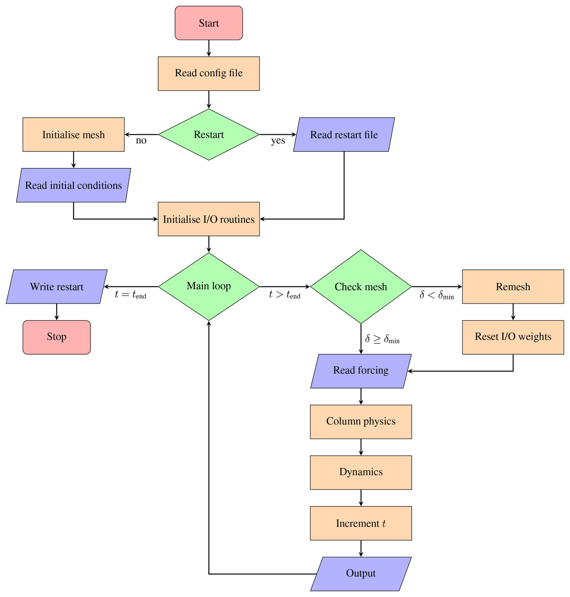
Figure 1 Program flow during an integration of neXtSIM. Purple parallelograms indicate I/O tasks, green triangles indicate boolean checks, and orange boxes indicate other tasks. Here, t indicates the model time and t_end the time at which the integration should stop. The smallest angle of any given triangle in the mesh is given by δ, and the smallest allowed such angle by δ_min.

2.1 Configuration files

NeXtSIM uses INI-style config files, which are read in using the |boost| |program_options| library. The neXtSIM config file is sorted into 18 sections: |simul|, |debugging|, |numerics|, |setup|, |mesh|, |moorings|, |drifters|, |restart|, |output|, |ideal_simul|, |dynamics|, |thermo|, |nesting|, |forecast|, |coupler|, |wave_coupling|, |statevector|, and |age|. Importantly, |simul| controls basic parameters of each simulation, such as start date and time step. The |setup| block sets the initial and boundary conditions, and |dynamics| and |thermo| control parameters and options for the model's dynamics and thermodynamics, respectively.

2.2 Initial conditions and restart files

Initial conditions are set depending on whether the user requests restarting from a previous model run or starting from a given set of initial conditions. The restart files are a set of custom binary files that describe both the model mesh and all required fields. Restart files are not guaranteed to work correctly if moved from one computer to another, although in practice, they will as long as the system's CPUs use the same endianness.

NeXtSIM supports a substantial number of different initial conditions when not starting from a restart file, through the |setup.ice-type| option. This includes reading in sea-ice thickness and concentration from the TOPAZ4, GLORYS, and PIOMAS reanalysis, as well as fields from AMSR2, AMSR2, IceSat, and CryoSat2 in various combinations.

2.3 Main loop

The main program loop consists of checking and updating the computational mesh, running the thermodynamics and dynamics routines, reading forcing fields, and outputting diagnostic and restart outputs. Mesh handling, thermodynamics, and dynamics are discussed in more detail in Sects. 5, 4, and 3. Here, it is important to note that remeshing impacts both reading of forcing files and writing to regularly spaced netCDF files.

While neXtSIM uses a Lagrangian moving mesh, the model assumes that the mesh remains static between remeshings for most input and output operations. In practice, this means that the functions that interpolate the input and output data between the mesh and the source or destination grids use interpolation weights that are recalculated only when the mesh is updated (see Sect. 5.1). This also holds for routines interfacing with the OASIS coupler. In addition to gridded outputs (Sect. 5.4), neXtSIM also provides outputs which are snapshots of the computational grid and preserve the instantaneous positions of the grid nodes. These files are written in the same customised format as the restart files. Finally, restart files are written at the end of the simulation or at given intervals, as requested by the user.

3 Dynamics

The core equation of sea-ice dynamics is the momentum equation. This is Newton's second law, but implementations may vary depending on the level of detail considered (e.g. Hibler, 1979; Connolley et al., 2004; Bouillon and Rampal, 2015; Danilov et al., 2015). The form used in neXtSIM is

$$\begin{array}{}\text{(1)}& m{\displaystyle \frac{\partial \mathit{u}}{\partial t}}=\mathbf{\nabla }\cdot \left(\mathit{\sigma }h\right)+A\left({\mathit{\tau }}_{\mathrm{a}}+{\mathit{\tau }}_{\mathrm{w}}\right)+{\mathit{\tau }}_{\mathrm{b}}+mf\mathit{k}\times \mathit{u}-mg\mathbf{\nabla }{H}_{\mathrm{o}},\end{array}$$

where A is the fraction of the grid cell covered by ice, m=Aρh is the ice mass per unit area, u is the ice velocity, σ is the internal stress tensor, h is the ice slab thickness (not volume per unit area), ρ the ice density, τ_a and τ_w are the atmosphere and ocean stress terms, respectively, ${\mathit{\tau }}_{\mathrm{b}}=-C_{\mathrm{b}}\mathit{u}$ is the basal stress term introduced in Lemieux et al. (2015), mfk×u is the Coriolis term, with vertical unit vector k, and mg∇H_o is the ocean-tilt term with g being the acceleration due to gravity and H_o the sea-surface height. We write the integrated internal stress explicitly as σh, following Sulsky et al. (2007) and Bouillon and Rampal (2015). Rheology determines the internal stress, σ, which links stress and strain, or strain rates, in the ice. The dynamical core of neXtSIM is built around a finite element discretisation of the momentum equation and a time-splitting approach for time-stepping the model equations.

One primary purpose of neXtSIM has been to explore the performance and effects of using the brittle rheologies (Girard et al., 2011; Dansereau et al., 2016; Ólason et al., 2022) in a large-scale context. In version 2 of neXtSIM, only the BBM rheology is included, out of the brittle rheologies. The EB and MEB rheologies can be recovered using an appropriate set of BBM parameters. Still, the interest in using EB and MEB for large-scale applications is, arguably, limited. In version 2 of neXtSIM, we also include implementations of the elasto-viscous-plastic (EVP) (Hunke and Dukowicz, 1997) and modified elasto-viscous-plastic (mEVP) (Lemieux et al., 2012; Bouillon et al., 2013) rheologies for comparison and testing.

3.1 Spatial discretisation

The finite element discretisation is based on a triangular grid, with ice velocities defined at the vertices and tracers treated as constant within the elements (consider e.g. Rao, 2007; Danilov et al., 2015; Bouillon and Rampal, 2015; Bielak, 2024, for details beyond what is given below). To solve the momentum equation in this framework, we define a set of test functions to obtain the weak formulation of the equation. Using a continuous Galerkin discretisation, we select the test functions, $N_j^e$, as linear functions associated with vertex j of element e of the triangular mesh. This function equals one at the vertex j and zero at all other vertices. The ice velocity field in element e is thus

$$\begin{array}{}\text{(2)}& \mathit{u}=\sum _{e\left(j\right)}{\mathit{u}}_j{N}_j^e,\end{array}$$

where the sum is over all the vertices of e.

The gradient of the velocity field is related to the gradient of the test functions, referred to here as the shape coefficients. These are calculated by defining the test functions on the three nodes of a reference element in the coordinates {ξ,υ}, as

$$\begin{array}{}\text{(3)}& {\displaystyle }& {\displaystyle }{N}_{\mathrm{1}}(\mathit{\xi },\mathit{\upsilon })=\mathrm{1}-\mathit{\xi }-\mathit{\upsilon }\text{(4)}& {\displaystyle }& {\displaystyle }{N}_{\mathrm{2}}(\mathit{\xi },\mathit{\upsilon })=\mathit{\xi }\text{(5)}& {\displaystyle }& {\displaystyle }{N}_{\mathrm{3}}(\mathit{\xi },\mathit{\upsilon })=\mathit{\upsilon },\end{array}$$

and then projecting this onto e using the transformation

$$\begin{array}{}\text{(6)}& \begin{array}{rl}x(\mathit{\xi },\mathit{\upsilon })& =N_{\mathrm{1}}^e{x}_{\mathrm{1}}^e+N_{\mathrm{2}}^e{x}_{\mathrm{2}}^e+N_{\mathrm{3}}^e{x}_{\mathrm{3}}^e\\ y(\mathit{\xi },\mathit{\upsilon })& =N_{\mathrm{1}}^e{y}_{\mathrm{1}}^e+N_{\mathrm{2}}^e{y}_{\mathrm{2}}^e+N_{\mathrm{3}}^e{y}_{\mathrm{3}}^e,\end{array}\end{array}$$

where the coordinates x_i and y_i are those of the three vertices of e. The shape coefficients are then computed as

$$\begin{array}{}\text{(7)}& {\displaystyle }\left[\begin{array}{c}\frac{\partial N_j^e}{\partial x}\\ \frac{\partial N_j^e}{\partial y}\end{array}\right]={\displaystyle \frac{\mathrm{1}}{\det \left(\mathbf{J}\right)}}\left[\begin{array}{ccc}{y}_{\mathrm{2}}-y_{\mathrm{3}}& y_{\mathrm{3}}-y_{\mathrm{1}}& y_{\mathrm{1}}-y_{\mathrm{2}}\\ x_{\mathrm{2}}-x_{\mathrm{3}}& x_{\mathrm{3}}-x_{\mathrm{1}}& x_{\mathrm{1}}-x_{\mathrm{3}}\end{array}\right],\end{array}$$

where det(J) is the determinant of the Jacobian of the transformation Eq. (6), computed as

$$\begin{array}{}\text{(8)}& \det \left(\mathbf{J}\right)=x_{\mathrm{2}}{y}_{\mathrm{3}}+x_{\mathrm{3}}{y}_{\mathrm{1}}+x_{\mathrm{1}}{y}_{\mathrm{2}}-x_{\mathrm{2}}{y}_{\mathrm{1}}-x_{\mathrm{3}}{y}_{\mathrm{2}}-x_{\mathrm{1}}{y}_{\mathrm{3}},\end{array}$$

and is equal to twice the element area. The coordinates x_i and y_i are taken to start at j and go around e in a counter-clockwise fashion.

The strain-rate equations can now be calculated using the shape coefficients. The strain-rate equations are

$$\begin{array}{}\text{(9)}& {\displaystyle }& {\displaystyle }{\dot{\mathit{\epsilon }}}_{\mathrm{11}}={\displaystyle \frac{\partial u}{\partial x}}\text{(10)}& {\displaystyle }& {\displaystyle }{\dot{\mathit{\epsilon }}}_{\mathrm{22}}={\displaystyle \frac{\partial v}{\partial y}}\text{(11)}& {\displaystyle }& {\displaystyle }{\dot{\mathit{\epsilon }}}_{\mathrm{12}}={\displaystyle \frac{\mathrm{1}}{\mathrm{2}}}\left({\displaystyle \frac{\partial u}{\partial y}}+{\displaystyle \frac{\partial v}{\partial x}}\right),\end{array}$$

where ${\dot{\mathit{\epsilon }}}_{ij}$ are the components of the strain-rate tensor $\dot{\mathit{\epsilon }}$, the dot symbolising the time derivative, and u and v are the zonal and meridional components of u. The strain-rate equations are projected onto the test functions to give element-wise strain rates:

$$\begin{array}{}\text{(12)}& {\displaystyle }& {\displaystyle }{\left({\dot{\mathit{\epsilon }}}_{\mathrm{11}}\right)}_e=\sum _{j\left(e\right)}\left(u_j{\displaystyle \frac{\partial N_j^e}{\partial x}}\right)\text{(13)}& {\displaystyle }& {\displaystyle }{\left({\dot{\mathit{\epsilon }}}_{\mathrm{22}}\right)}_e=\sum _{j\left(e\right)}\left(v_j{\displaystyle \frac{\partial N_j^e}{\partial y}}\right)\text{(14)}& {\displaystyle }& {\displaystyle }{\left({\dot{\mathit{\epsilon }}}_{\mathrm{12}}\right)}_e=\sum _{j\left(e\right)}\left(u_j{\displaystyle \frac{\partial N_j^e}{\partial y}}+v_j{\displaystyle \frac{\partial N_j^e}{\partial x}}\right).\end{array}$$

In neXtSIM, we solve the equations on an {x,y} plane (usually using a polar stereographic projection), so we do not need to account for metric terms that arise due to the curvature of the earth.

To solve the momentum equation, we follow Danilov et al. (2015) and use nodal quadrature in all terms that do not involve spatial derivatives. This allows us to solve the BBM, EVP, and mEVP models efficiently using explicit time stepping. Multiplying the momentum equation by the test functions, integrating over the domain, and integrating the rheology term by parts gives the following at vertex j:

$$\begin{array}{}\text{(15)}& \begin{array}{rl}\int m& N_j\left({\displaystyle \frac{\partial \mathit{u}}{\partial t}}\right)\mathrm{d}S=\int N_{j}h\mathbf{n}\mathit{\sigma }\mathrm{d}\mathrm{\Gamma }-\int \left(\mathrm{\nabla }{N}_j\right)h\mathit{\sigma }\mathrm{d}S\\ & +\int N_j\left[A\left({\mathit{\tau }}_{\mathrm{a}}+{\mathit{\tau }}_{\mathrm{w}}\right)+{\mathit{\tau }}_{\mathrm{b}}+f\mathbf{k}\times \mathit{u}\right]\mathrm{d}S\\ & -\int mg\mathrm{\nabla }{H}_{\mathrm{o}}{N}_j\mathrm{d}S,\end{array}\end{array}$$

where S is the domain, Γ the boundary of the domain and n the normal vector to that boundary.

The numerical integration of Eq. (15) proceeds as follows: The left-hand side can be written as

$$\begin{array}{}\text{(16)}& \int m{N}_j\left({\displaystyle \frac{\partial \mathit{u}}{\partial t}}\right)\mathrm{d}S=\sum _k{M}_{jk}{m}_k\left({\displaystyle \frac{\partial {\mathit{u}}_k}{\partial t}}\right),\end{array}$$

where the summation is taken over all vertices, k. The lump mass matrix, M is diagonal and its non-zero entries are

$$\begin{array}{}\text{(17)}& M_{ii}={\displaystyle \frac{\mathrm{1}}{\mathrm{3}}}\sum _{e\left(i\right)}{A}_e,\end{array}$$

where the sum is taken over all elements containing the vertex i. The nodal mass m_j is calculated as the area-weighted mean of all the neighbouring element thickness values. The left-hand side then becomes simply

$$\begin{array}{}\text{(18)}& \int m{N}_j\left({\displaystyle \frac{\partial \mathit{u}}{\partial t}}\right)\mathrm{d}S=m_j\left({\displaystyle \frac{\partial {\mathit{u}}_j}{\partial t}}\right)M_{jj}.\end{array}$$

Similarly, the third term on the right-hand side becomes

$$\begin{array}{}\text{(19)}& \begin{array}{rl}\int N_j& \left[A\left({\mathit{\tau }}_{\mathrm{a}}+{\mathit{\tau }}_{\mathrm{w}}\right)+{\mathit{\tau }}_{\mathrm{b}}+f\mathbf{k}\times \mathit{u}\right]\mathrm{d}.\\ & =\left[A{\left({\mathit{\tau }}_{\mathrm{a}}S+{\mathit{\tau }}_{\mathrm{w}}\right)}_j+{\left({\mathit{\tau }}_{\mathrm{b}}\right)}_j+f\mathbf{k}\times {\mathit{u}}_j\right]M_{jj}.\end{array}\end{array}$$

The first term on the right-hand side is the boundary contribution, which we set to zero under the assumption of a no-slip boundary condition.

The second and fourth terms on the right-hand side – the internal stress term and sea-surface tilt term, respectively – are more involved than the terms already discussed and require summation over the elements e(j) surrounding j. The x-component of the internal stress term becomes

$$\begin{array}{}\text{(20)}& \begin{array}{rl}{\left[-\int \left(\mathrm{\nabla }{N}_j\right)h\mathit{\sigma }\mathrm{d}S\right]}_x& =-{\displaystyle \frac{\mathrm{1}}{\mathrm{3}}}\sum _{e\left(j\right)}{A}_e{h}_e\left({\left({\mathit{\sigma }}_{\mathrm{11}}\right)}_e{\displaystyle \frac{\partial N_j}{\partial x}}\right.\\ & \left.+{\left({\mathit{\sigma }}_{\mathrm{12}}\right)}_e{\displaystyle \frac{\partial N_j}{\partial y}}\right)\end{array}\end{array}$$

and the y-component becomes

$$\begin{array}{}\text{(21)}& \begin{array}{rl}{\left[-\int \left(\mathrm{\nabla }{N}_j\right)h\mathit{\sigma }\mathrm{d}S\right]}_y& =-{\displaystyle \frac{\mathrm{1}}{\mathrm{3}}}\sum _{e\left(j\right)}{A}_e{h}_e\left({\left({\mathit{\sigma }}_{\mathrm{12}}\right)}_e{\displaystyle \frac{\partial N_j}{\partial x}}\right.\\ & \left.+{\left({\mathit{\sigma }}_{\mathrm{11}}\right)}_e{\displaystyle \frac{\partial N_j}{\partial y}}\right),\end{array}\end{array}$$

with σ_ij the components of the stress tensor σ. The sea-surface tilt term requires a double summation, where the x-component becomes

$$\begin{array}{}\text{(22)}& {\left(-\int mg\mathrm{\nabla }{H}_{\mathrm{o}}{N}_j\mathrm{d}S\right)}_x=g{m}_j{\displaystyle \frac{\mathrm{1}}{\mathrm{3}}}\sum _{e\left(j\right)}\left(A_e\sum _{k\left(e\right)}{H}_{\mathrm{o},k}{\displaystyle \frac{\partial N_k}{\partial x}}\right)\end{array}$$

and the y-component

$$\begin{array}{}\text{(23)}& {\left(-\int mg\mathrm{\nabla }{H}_{\mathrm{o}}{N}_j\mathrm{d}S\right)}_y=g{m}_j{\displaystyle \frac{\mathrm{1}}{\mathrm{3}}}\sum _{e\left(j\right)}\left(A_e\sum _{k\left(e\right)}{H}_{\mathrm{o},k}{\displaystyle \frac{\partial N_k}{\partial y}}\right).\end{array}$$

3.2 Temporal discretisation

The time-splitting method we use in neXtSIM is based on that proposed by Hunke and Dukowicz (1997) for the EVP model, where they solve the column physics and advection equations on the main model time step Δt, but apply a sub-time stepping to solve the momentum equation at a shorter time step, Δt_m. In neXtSIM, we use this time-stepping scheme for the BBM (as in Ólason et al., 2022) and the EVP model, whereas the mEVP requires a small modification to the time-stepping and internal stress calculation (see Sect. 3.4).

The time stepping of the momentum equation follows the semi-implicit solution derived by Hunke and Dukowicz (1997). Following the discretisation discussion above, this then takes the form

$$\begin{array}{}\text{(24)}& \begin{array}{rl}\left({\mathit{\alpha }}^{\mathrm{2}}+{\mathit{\beta }}^{\mathrm{2}}\right)u_j^{n+\mathrm{1}}=& \mathit{\alpha }{u}_j+\mathit{\beta }{v}_j+{\displaystyle \frac{\mathrm{\Delta }{t}_{\mathrm{m}}}{m_j{M}_{jj}}}\\ & \left[\mathit{\alpha }\left({\left[-\int \left(\mathrm{\nabla }{N}_j\right)h_j\mathit{\sigma }\mathrm{d}S\right]}_x+{\mathit{\tau }}_x\right)\right.\\ & \left.+\mathit{\beta }\left({\left[-\int \left(\mathrm{\nabla }{N}_j\right)h_j\mathit{\sigma }\mathrm{d}S\right]}_y+{\mathit{\tau }}_y\right)\right]\end{array}\end{array}$$

and (correcting for a sign error in Hunke and Dukowicz, 1997 on the last β term)

$$\begin{array}{}\text{(25)}& \begin{array}{rl}\left({\mathit{\alpha }}^{\mathrm{2}}+{\mathit{\beta }}^{\mathrm{2}}\right)u_j^{n+\mathrm{1}}=& \mathit{\alpha }{u}_j-\mathit{\beta }{v}_j+{\displaystyle \frac{\mathrm{\Delta }{t}_{\mathrm{m}}}{m_j{M}_{jj}}}\\ & \left[\mathit{\alpha }\left({\left[-\int \left(\mathrm{\nabla }{N}_j\right)h_j\mathit{\sigma }\mathrm{d}S\right]}_y+{\mathit{\tau }}_y\right)\right.\\ & \left.-\mathit{\beta }\left({\left[-\int \left(\mathrm{\nabla }{N}_j\right)h_j\mathit{\sigma }\mathrm{d}S\right]}_x+{\mathit{\tau }}_x\right)\right]\end{array}\end{array}$$

where all values on the right-hand side are taken at time n to produce u and v at time n+1 on the left-hand side. The integrals are calculated following Eqs. (20) and (21). Additionally we have

$$\begin{array}{}\text{(26)}& {\displaystyle }& {\displaystyle }{c}^{\prime }={\mathit{\rho }}_{\mathrm{w}}{C}_{\mathrm{w}}|{\mathit{u}}_{\mathrm{w}}-\mathit{u}|\text{(27)}& {\displaystyle }& {\displaystyle }\mathit{\alpha }=\mathrm{1}+{\displaystyle \frac{\mathrm{\Delta }{t}_{\mathrm{m}}}{m_j}}\left(c^{\prime }\cos {\mathit{\theta }}_{\mathrm{w}}+C_{\mathrm{b}}\right)\text{(28)}& {\displaystyle }& {\displaystyle }\mathit{\beta }=\mathrm{\Delta }{t}_{\mathrm{m}}\left(f+{\displaystyle \frac{c^{\prime }\sin {\mathit{\theta }}_{\mathrm{w}}}{m_j}}\right)\end{array}$$

and

$$\begin{array}{}\text{(29)}& {\displaystyle }& {\displaystyle }{\mathit{\tau }}_x={\mathit{\tau }}_{\mathrm{a},x}+c^{\prime }\left(u_{\mathrm{w}}\cos {\mathit{\theta }}_{\mathrm{w}}-v_{\mathrm{w}}\sin {\mathit{\theta }}_{\mathrm{w}}\right)-{\left(\int mg\mathrm{\nabla }{H}_{\mathrm{o}}{N}_j\mathrm{d}S\right)}_x\text{(30)}& {\displaystyle }& {\displaystyle }{\mathit{\tau }}_y={\mathit{\tau }}_{\mathrm{a},y}+c^{\prime }\left(v_{\mathrm{w}}\cos {\mathit{\theta }}_{\mathrm{w}}-u_{\mathrm{w}}\sin {\mathit{\theta }}_{\mathrm{w}}\right)-{\left(\int mg\mathrm{\nabla }{H}_{\mathrm{o}}{N}_j\mathrm{d}S\right)}_y,\end{array}$$

where the integrals are calculated following Eqs. (20) to (23). Here, ρ_w is the ocean water density, C_w the ice-ocean drag coefficient, u_w the ocean velocity (and u_w and v_w its components), θ_w the ocean turning angle, and τ_a,x and τ_a,y are the x and y components of the ice-ocean stress

$$\begin{array}{}\text{(31)}& \mathit{\tau }={\mathit{\rho }}_{\mathrm{a}}{C}_{\mathrm{m}}\left|\mathit{u}\right|\mathit{u},\end{array}$$

with ρ_a the atmospheric density and C_m the atmospheric drag coefficient for momentum exchange (e.g. Leppäranta, 2011).

3.3 BBM implementation

The Brittle Bingham-Maxwell rheology (BBM) is described in detail in Ólason et al. (2022); here we briefly discuss it for completeness, focusing on aspects relevant to neXtSIM. The BBM rheology is a damaging Bingham-Maxwell constitutive model. Using damage mechanics for sea-ice modelling was introduced with the elasto-brittle (EB) model by Girard et al. (2011), but damage mechanics are widely used in other communities, e.g. in rock and crustal mechanics (e.g. Lyakhovsky et al., 1997; Amitrano et al., 1999; Schapery, 1999)).

The EB model simulates the ice as a damaging elastic sheet, where each grid element can be considered a spring in a mechanics sense. In the EB model, the stress is calculated in every grid cell, and if the stress is outside the Mohr–Coulomb yield criterion, the elasticity is reduced in that grid cell, and the sea ice experiences a reversible deformation. The Mohr–Coulomb criterion is

$$\begin{array}{}\text{(32)}& \mathit{\tau }={\mathit{\sigma }}_{\mathrm{N}}\mathit{\mu }+C,\end{array}$$

where μ is a constant friction coefficient, C, is the material cohesion, and τ and σ_N are the shear and normal stresses:

$$\begin{array}{}\text{(33)}& {\displaystyle }& {\displaystyle }\mathit{\tau }={\displaystyle \frac{\mathrm{1}}{\mathrm{2}}}\sqrt{{\left({\mathit{\sigma }}_{\mathrm{11}}-{\mathit{\sigma }}_{\mathrm{22}}\right)}^{\mathrm{2}}+\mathrm{4}{\mathit{\tau }}_{\mathrm{12}}^{\mathrm{2}}}\text{(34)}& {\displaystyle }& {\displaystyle }{\mathit{\sigma }}_{\mathrm{N}}={\displaystyle \frac{\mathrm{1}}{\mathrm{2}}}\left({\mathit{\sigma }}_{\mathrm{11}}+{\mathit{\sigma }}_{\mathrm{22}}\right).\end{array}$$

Elasticity, E, in the model is thus

$$\begin{array}{}\text{(35)}& E=Y(\mathrm{1}-d),\end{array}$$

where Y is the ice's Young modulus, and d with $\mathrm{0}\le d<\mathrm{1}$, is a scalar damage variable.

At the start of the simulation, d=0 everywhere, but d is then increased to ensure that all stresses in the ice are always within the yield criterion. A local increase in d represents damaging of the ice, which is modelled as a reduction in elasticity. The reduction in elasticity in an element means that this element deforms more easily than before, and so the distribution of stresses in the neighbouring elements must change. This causes a stress redistribution and a cascade of damage increases, emulating the multiplicative cascade that Marsan et al. (2004) suggested was the reason for the spatial scaling of sea-ice deformation they observed in satellite remote sensing data.

The MEB model (Dansereau et al., 2016) introduced a viscous element, or a dashpot, in series with the elastic one. This is intended to simulate the viscous dissipation of internal stresses and the larger, irreversible deformations (as opposed to the elastic counterpart) that occur along faults once the material is highly damaged. The viscosity of the dashpot is very high when the ice is undamaged, but should decrease faster than the spring's elasticity when damage increases. This is formulated as:

$$\begin{array}{}\text{(36)}& \mathit{\eta }={\mathit{\eta }}_{\mathrm{0}}(\mathrm{1}-d{)}^{\mathit{\alpha }},\end{array}$$

where η is the dashpot's viscosity, α is a material-dependent constant, and η₀ is the viscosity of undamaged ice. This should tend towards infinity, but is set to 10⁷ s⁻¹ for practical purposes.

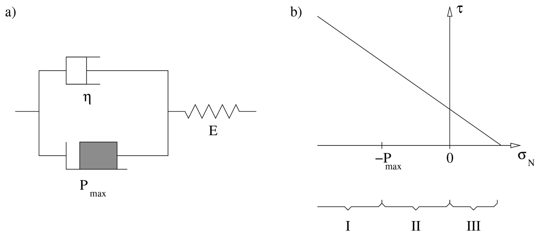
Figure 2 (a) A schematic of the Bingham–Maxwell constitutive model showing a dashpot and a friction element connected in parallel, with both connected to a spring in series. (b) The yield criterion in the stress invariant plane {σ_N,τ}, as well as the elastic limit P_max, and the ridging (I), elastic (II), and diverging (III) regimes.

The Bingham–Maxwell model consists of a friction block and a dashpot in parallel, connected with a spring in serial. A schematic of the constitutive model is shown in panel a of Fig. 2. The spring's elasticity and the dashpot's viscosity evolve as a function of the damage variable, as in the MEB rheology. The friction element is introduced to emulate the resistance to ridging, so that, for small compressive stresses, the ice remains fully elastic regardless of the level of damage. This leads to the model having three regimes in stress space: a visco-elastic converging one for high compressive normal stress, a purely elastic one for compressive normal stress less than the threshold P_max, and a visco-elastic diverging one for divergent normal stress. These three regimes are shown schematically in of Fig. 2b.

The constitutive equation for BBM is

$$\begin{array}{}\text{(37)}& \dot{\mathit{\sigma }}=E\mathbf{K}:\dot{\mathit{\epsilon }}-{\displaystyle \frac{\mathit{\sigma }}{\mathit{\lambda }}}\left(\mathrm{1}+\stackrel{\mathrm{̃}}{P}+{\displaystyle \frac{\mathit{\lambda }\dot{d}}{\mathrm{1}-d}}\right),\end{array}$$

where σ and $\dot{\mathit{\epsilon }}$ are the stress and strain rate tensors, respectively, $\mathit{\lambda }=\mathit{\eta }/E={\mathit{\lambda }}_{\mathrm{0}}(\mathrm{1}-d{)}^{\mathit{\alpha }-\mathrm{1}}$ is the viscous relaxation time, with ${\mathit{\lambda }}_{\mathrm{0}}={\mathit{\eta }}_{\mathrm{0}}/Y$ the undamaged viscous relaxation time. We assume plane stress conditions, so the stiffness tensor operation $\mathbf{K}:\dot{\mathit{\epsilon }}$ is

$$\begin{array}{}\text{(38)}& \left(\begin{array}{c}{\left(\mathbf{K}:\dot{\mathit{\epsilon }}\right)}_{\mathrm{11}}\\ {\left(\mathbf{K}:\dot{\mathit{\epsilon }}\right)}_{\mathrm{22}}\\ {\left(\mathbf{K}:\dot{\mathit{\epsilon }}\right)}_{\mathrm{12}}\end{array}\right)={\displaystyle \frac{\mathrm{1}}{\mathrm{1}-{\mathit{\nu }}^{\mathrm{2}}}}\left(\begin{array}{ccc}\mathrm{1}& \mathit{\nu }& \mathrm{0}\\ \mathit{\nu }& \mathrm{1}& \mathrm{0}\\ \mathrm{0}& \mathrm{0}& \mathrm{1}-\mathit{\nu }\end{array}\right)\left(\begin{array}{c}{\dot{\mathit{\epsilon }}}_{\mathrm{11}}\\ {\dot{\mathit{\epsilon }}}_{\mathrm{22}}\\ {\dot{\mathit{\epsilon }}}_{\mathrm{12}}\end{array}\right)\end{array}$$

where ν is Poisson's ratio. The resistance to ridging is encoded in $\stackrel{\mathrm{̃}}{P}$ as

$$\begin{array}{}\text{(39)}& {\displaystyle }{\displaystyle }\stackrel{\mathrm{̃}}{P}=\left\{\begin{array}{ll}\frac{P_{\max }}{{\mathit{\sigma }}_{\mathrm{N}}}& \mathrm{for}{\mathit{\sigma }}_{\mathrm{N}}<-P_{\max }\\ -\mathrm{1}& \mathrm{for}-P_{\max }<{\mathit{\sigma }}_{\mathrm{N}}<\mathrm{0}\\ \mathrm{0}& \mathrm{for}{\mathit{\sigma }}_{\mathrm{N}}>\mathrm{0}\end{array}\right.\end{array}$$

where

$$\begin{array}{}\text{(40)}& P_{\max }=P{\left({\displaystyle \frac{h}{h_{\mathrm{0}}}}\right)}^f{e}^{-C(\mathrm{1}-A)},\end{array}$$

with P a constant ice strength parameter, h₀=1 m, A is ice concentration and C is a constant regulating the decrease of P_max as the concentration decreases. The factor $f\in [\mathrm{1},\mathrm{2}]$ was set to $f=\mathrm{3}/\mathrm{2}$ by Ólason et al. (2022), who also briefly explored the impact of varying f. The three cases for $\stackrel{\mathrm{̃}}{P}$ correspond to the cases I, II, and III in Fig. 2b, corresponding to visco-elastic (ridging), pure elastic, and diverging regimes. Equation (40) for P_max determines the compressive stress required to move from the elastic to the visco-elastic regime, i.e. when the ice can ridge.

Equation (37) is solved together with the momentum equation using Eqs. (24) and (25). The time stepping of Eq. (37) is done in two steps. First, we calculate an intermediate stress, σ^′ through an Euler forwards iteration of Eq. (37), assuming $\dot{d}=\mathrm{0}$, wich gives

$$\begin{array}{}\text{(41)}& {\displaystyle \frac{{\mathit{\sigma }}^{\prime }-{\mathit{\sigma }}^n}{\mathrm{\Delta }t}}=E\mathbf{K}:\dot{\mathit{\epsilon }}-{\displaystyle \frac{{\mathit{\sigma }}^{\prime }}{\mathit{\lambda }}}\left(\mathrm{1}+\stackrel{\mathrm{̃}}{P}\right),\end{array}$$

or, after rearranging

$$\begin{array}{}\text{(42)}& {\mathit{\sigma }}^{\prime }={\displaystyle \frac{\mathit{\lambda }\left(\mathrm{\Delta }{t}_{\mathrm{m}}E\mathbf{K}:\dot{\mathit{\epsilon }}+{\mathit{\sigma }}^n\right)}{\mathit{\lambda }+\mathrm{\Delta }{t}_{\mathrm{m}}\left(\mathrm{1}+\stackrel{\mathrm{̃}}{P}\right)}},\end{array}$$

where σⁿ is the stress at the start of the time step.

If σ^′ is outside the yield criterion, an updated damage value is calculated as

$$\begin{array}{}\text{(43)}& d^{n+\mathrm{1}}=d^n+\left(\mathrm{1}-d_{\mathrm{crit}}\right)\left(\mathrm{1}-d^n\right),\end{array}$$

and a consistent stress correction is applied

$$\begin{array}{}\text{(44)}& {\mathit{\sigma }}^{n+\mathrm{1}}={\mathit{\sigma }}^{\prime }{d}_{\mathrm{crit}}.\end{array}$$

Here, d_crit is the factor needed to relax the stresses back onto the yield criterion, which is calculated as

$$\begin{array}{}\text{(45)}& d_{\mathrm{crit}}=\left\{\begin{array}{ll}-N/{\mathit{\sigma }}_{\mathrm{N}}& \mathrm{if}{\mathit{\sigma }}_{\mathrm{N}}<-N,\\ c/\left(\mathit{\tau }+\mathit{\mu }{\mathit{\sigma }}_{\mathrm{N}}\right)& \mathrm{if}\mathit{\tau }>c-\mathit{\mu }{\mathit{\sigma }}_{\mathrm{N}},\end{array}\right.\end{array}$$

where c and μ are the cohesion and internal friction coefficient values for the Mohr–Coulomb criterion, respectively. A capping with a large value of N is needed to prevent numerical instabilities (see Plante et al., 2020), where N is chosen sufficiently large to avoid affecting the solution. In neXtSIM, the default value is four orders of magnitude larger than the cohesion. Equation (45) follows the damaging scheme of Bouillon and Rampal (2015) rather than that of Dansereau et al. (2016), as Ólason et al. (2022) did. The consequences of which scheme is chosen are discussed in Sect. 6.1. If σ^′ is inside the yield criterion, i.e. d_crit<0 or d_crit>1, damage remains unchanged and σⁿ⁺¹ is set to σ^′.

We note that the finite-element discretisation used in neXtSIM results in the co-location of all the stress tensor components. This co-location is advantageous for the BBM implementation, because all stress tensor components are needed to calculate σ_N and τ of Eq. (45). Models using a staggered grid, where different components of the stress tensor lie at different locations (e.g. the B- or C-grid) must apply extra effort to achieve the co-location of the stress components needed to get an accurate estimate of d_crit (e.g. Plante et al., 2020; Brodeau et al., 2024).

3.4 EVP and mEVP implementation

The elasto-viscous-plastic (EVP Hunke and Dukowicz, 1997) and the modified elasto-viscous-plastic (mEVP Lemieux et al., 2012; Bouillon et al., 2013) rheologies are numerically efficient and easily parallelisable approaches to solving the equations of the original visco-plastic rheology (VP Hibler, 1979). In the VP model, the internal stress tensor is diagnosed from the strain rates as

$$\begin{array}{}\text{(46)}& {\displaystyle }& {\displaystyle }{\mathit{\sigma }}_{\mathrm{N}}=\mathit{\zeta }{\dot{\mathit{\epsilon }}}_{\mathrm{I}}-P/\mathrm{2}\text{(47)}& {\displaystyle }& {\displaystyle }\mathit{\tau }=\mathit{\eta }{\dot{\mathit{\epsilon }}}_{\mathrm{II}}\end{array}$$

where

$$\begin{array}{}\text{(48)}& {\displaystyle }& {\displaystyle }{\dot{\mathit{\epsilon }}}_{\mathrm{I}}={\displaystyle \frac{\mathrm{1}}{\mathrm{2}}}\left({\dot{\mathit{\epsilon }}}_{\mathrm{11}}+{\dot{\mathit{\epsilon }}}_{\mathrm{22}}\right)\text{(49)}& {\displaystyle }& {\displaystyle }{\dot{\mathit{\epsilon }}}_{\mathrm{II}}={\displaystyle \frac{\mathrm{1}}{\mathrm{2}}}\sqrt{{\left({\dot{\mathit{\epsilon }}}_{\mathrm{11}}-{\dot{\mathit{\epsilon }}}_{\mathrm{22}}\right)}^{\mathrm{2}}+\mathrm{4}{\dot{\mathit{\epsilon }}}_{\mathrm{12}}^{\mathrm{2}}}\end{array}$$

are the first and second strain rate invariants and

$$\begin{array}{}\text{(50)}& {\displaystyle }& {\displaystyle }\mathit{\zeta }={\displaystyle \frac{P}{\mathrm{2}\mathrm{\Delta }+{\mathrm{\Delta }}_{\min }}}\text{(51)}& {\displaystyle }& {\displaystyle }\mathit{\eta }=\mathit{\zeta }/e^{\mathrm{2}}\text{(52)}& {\displaystyle }& {\displaystyle }\mathrm{\Delta }=\sqrt{{\dot{\mathit{\epsilon }}}_{\mathrm{I}}^{\mathrm{2}}+{\dot{\mathit{\epsilon }}}_{\mathrm{II}}^{\mathrm{2}}/e^{\mathrm{2}}}\text{(53)}& {\displaystyle }& {\displaystyle }P=P^{*}h{e}^{-C(\mathrm{1}-A)}\end{array}$$

with e and P^* constants controlling the ellipse eccentricity and the ice strength, and Δ_min a constant regulating the maximum viscosity in the model.

The VP equations must be solved implicitly using an iterative scheme, such as a fixed-point iteration or a Picard solver. To avoid using an implicit solver, Hunke and Dukowicz (1997) introduced an elastic term, which allows the equations to be solved explicitly through sub-iterations. The VP rheology is recovered as the steady state limit of the EVP rheology of Hunke and Dukowicz (1997) or in the limit of an infinitely large elasticity. For the EVP, the momentum equation is solved using the explicit time-stepping scheme detailed above in Eqs. (24) and (25).

In neXtSIM, we follow Bouillon et al. (2013) in solving the EVP constituent equations by defining ${\mathit{\sigma }}_{\mathrm{1}}={\mathit{\sigma }}_{\mathrm{11}}+{\mathit{\sigma }}_{\mathrm{22}}$ and ${\mathit{\sigma }}_{\mathrm{2}}={\mathit{\sigma }}_{\mathrm{11}}-{\mathit{\sigma }}_{\mathrm{22}}$ and solving for those as

$$\begin{array}{}\text{(54)}& {\displaystyle }& {\displaystyle }{\mathit{\sigma }}_{\mathrm{1}}^{n+\mathrm{1}}={\mathit{\sigma }}_{\mathrm{1}}^n+\left(\mathrm{2}\mathit{\zeta }\left[{\mathit{\epsilon }}_{\mathrm{11}}+{\mathit{\epsilon }}_{\mathrm{22}}-\mathrm{\Delta }\right]-{\mathit{\sigma }}_{\mathrm{1}}^n\right)/{\mathit{\alpha }}_{\mathrm{1}}\text{(55)}& {\displaystyle }& {\displaystyle }{\mathit{\sigma }}_{\mathrm{2}}^{n+\mathrm{1}}={\mathit{\sigma }}_{\mathrm{2}}^n+\left(\mathrm{2}\mathit{\zeta }\left[{\mathit{\epsilon }}_{\mathrm{11}}-{\mathit{\epsilon }}_{\mathrm{22}}\right]/e^{\mathrm{2}}-{\mathit{\sigma }}_{\mathrm{2}}^n\right)/{\mathit{\alpha }}_{\mathrm{2}}\text{(56)}& {\displaystyle }& {\displaystyle }{\mathit{\sigma }}_{\mathrm{12}}^{n+\mathrm{1}}={\mathit{\sigma }}_{\mathrm{12}}^n+\left(\mathrm{2}\mathit{\zeta }{\mathit{\epsilon }}_{\mathrm{12}}/e^{\mathrm{2}}-{\mathit{\sigma }}_{\mathrm{12}}^n\right)/{\mathit{\alpha }}_{\mathrm{2}},\end{array}$$

where ${\mathit{\alpha }}_{\mathrm{1}}=\mathrm{2}T/\mathrm{\Delta }{t}_{\mathrm{m}}$ and ${\mathit{\alpha }}_{\mathrm{2}}={\mathit{\alpha }}_{\mathrm{1}}/e^{\mathrm{2}}$, with $T=\mathrm{\Delta }t/\mathrm{3}$ as the elastic time scale.

From a technical standpoint, the mEVP consists of slight modifications of the time stepping of both the momentum and constituent equations of EVP. The constituent equations of mEVP are the same as for EVP (namely Eqs. 54–56), except we set ${\mathit{\alpha }}_{\mathrm{1}}={\mathit{\alpha }}_{\mathrm{2}}={\mathit{\alpha }}^{\prime }$, where α^′ is a constant tuning parameter introduced (as just α) by Bouillon et al. (2013). In neXtSIM, we take advantage of this similarity to reduce code duplication.

We also exploit similarities between the EVP/BBM momentum solver and the mEVP solver to reduce code duplication. For mEVP, the momentum equation time stepping takes the form

$$\begin{array}{}\text{(57)}& \begin{array}{rl}{\mathit{\beta }}^{\prime }{\displaystyle \frac{m}{\mathrm{\Delta }{t}_{\mathrm{m}}}}& \left({\mathit{u}}^{n+\mathrm{1}}-{\mathit{u}}^n\right)={\displaystyle \frac{m}{\mathrm{\Delta }{t}_{\mathrm{m}}}}\left({\mathit{u}}^{\mathrm{0}}-{\mathit{u}}^{n+\mathrm{1}}\right)+\mathbf{\nabla }\cdot \left(\mathit{\sigma }h\right)\\ & +A\left({\mathit{\tau }}_{\mathrm{a}}+{\mathit{\tau }}_{\mathrm{w}}\right)+{\mathit{\tau }}_{\mathrm{b}}+mf\mathit{n}\times \mathit{u}-mg\mathbf{\nabla }\mathit{\eta },\end{array}\end{array}$$

where β^′ is the numerical tuning parameter introduced (as just β) by Bouillon et al. (2013), u⁰ is the ice velocity at the start of the sub iterations, and uⁿ and uⁿ⁺¹ are the velocities at the previous and current sub-iteration step, respectively. Using the approach of Hunke and Dukowicz (1997), this can be rewritten as modified versions of Eqs. (24) and (25):

$$\begin{array}{}\text{(58)}& \begin{array}{rl}\left({\mathit{\alpha }}^{\mathrm{2}}+{\mathit{\beta }}^{\mathrm{2}}\right)& u_j^{n+\mathrm{1}}=\mathit{\alpha }{u}_j+\mathit{\beta }{v}_j+\mathit{\alpha }{\displaystyle \frac{u_j^{\mathrm{0}}-u_j^n}{b}}+\mathit{\beta }{\displaystyle \frac{v_j^{\mathrm{0}}-v_j^n}{b}}\\ & +{\displaystyle \frac{\mathrm{\Delta }{t}_{\mathrm{m}}}{b{m}_j{M}_{jj}}}\left[\mathit{\alpha }\left({\left[-\int \left(\mathrm{\nabla }{N}_j\right)h_j\mathit{\sigma }\mathrm{d}S\right]}_x+{\mathit{\tau }}_x\right)\right.\\ & \left.+\mathit{\beta }\left({\left[-\int \left(\mathrm{\nabla }{N}_j\right)h_j\mathit{\sigma }\mathrm{d}S\right]}_y+{\mathit{\tau }}_y\right)\right]\end{array}\end{array}$$

and

$$\begin{array}{}\text{(59)}& \begin{array}{rl}\left({\mathit{\alpha }}^{\mathrm{2}}+{\mathit{\beta }}^{\mathrm{2}}\right)& v_j^{n+\mathrm{1}}=\mathit{\alpha }{v}_j-\mathit{\beta }{u}_j+\mathit{\alpha }{\displaystyle \frac{v_j^{\mathrm{0}}-v_j^n}{b}}-\mathit{\beta }{\displaystyle \frac{u_j^{\mathrm{0}}-u_j^n}{b}}\\ & +{\displaystyle \frac{\mathrm{\Delta }{t}_{\mathrm{m}}}{b{m}_j{M}_{jj}}}\left[\mathit{\alpha }\left({\left[-\int \left(\mathrm{\nabla }{N}_j\right)h_j\mathit{\sigma }\mathrm{d}S\right]}_y+{\mathit{\tau }}_y\right)\right.\\ & \left.-\mathit{\beta }\left({\left[-\int \left(\mathrm{\nabla }{N}_j\right)h_j\mathit{\sigma }\mathrm{d}S\right]}_x+{\mathit{\tau }}_x\right)\right],\end{array}\end{array}$$

where $b={\mathit{\beta }}^{\prime }+\mathrm{1}$ and α and β become

$$\begin{array}{}\text{(60)}& {\displaystyle }& {\displaystyle }\mathit{\alpha }=\mathrm{1}+{\displaystyle \frac{\mathrm{\Delta }{t}_{\mathrm{m}}}{b{m}_j}}\left(c^{\prime }\cos {\mathit{\theta }}_{\mathrm{w}}+C_{\mathrm{b}}\right)\text{(61)}& {\displaystyle }& {\displaystyle }\mathit{\beta }={\displaystyle \frac{\mathrm{\Delta }{t}_{\mathrm{m}}}{b}}\left(f+{\displaystyle \frac{c^{\prime }\sin {\mathit{\theta }}_{\mathrm{w}}}{m_j}}\right).\end{array}$$

Importantly, the BBM and EVP equations are recovered by setting b=1 and u⁰=uⁿ.

In neXtSIM, switching between the BBM and mEVP rheologies is done by calling separate functions to calculate the stress tensor, σ. The momentum equation is then solved using Eqs. (58) and (59), setting ${\mathit{\beta }}^{\prime }=-\mathrm{1}$ and u⁰=uⁿ when using BBM or EVP.

4 Thermodynamics and column physics

The thermodynamics and column physics in neXtSIM are relatively simple compared to other sea-ice models, focusing on representing the processes most likely to be of interest when using brittle rheology, e.g. atmosphere–ocean–ice interactions in leads and polynyas. In addition, a diagnostic ridge ratio scheme is implemented in the model for the benefit of the sea-ice forecasting platform, neXtSIM-F (Williams et al., 2021) and a melt-pond scheme to improve long-term simulations, such as those of Boutin et al. (2023) and Regan et al. (2023). An ice-age tracer was implemented for Regan et al. (2023), with subsequent minor improvements.

4.1 Ice categories

In general, a sea–ice model's grid cell must be divided into at least two categories: ice and open water (e.g. Hibler, 1979). Many models also use categories of different ice thicknesses, with five thickness categories being a common choice (e.g. Bitz et al., 2001; Hunke and Lipscomb, 2010; Rousset et al., 2015; Adcroft et al., 2019). Contrary to pure thickness categories, neXtSIM includes a multi-category model based on state of development, considering three categories: consolidated ice, young ice and open water (see Appendix A2 of Rampal et al., 2019, who refer to the categories as “thick” and “thin” and not “consolidated” and “young”).

In this model, young ice is described by its concentration, A_y, volume per unit area, H_y, and snow volume per unit area, H_s,y. Consolidated ice is described by the concentration, A, volume per unit area, H, and snow volume per unit area, H_s. We assume that the young ice has no mechanical strength and simply follows the motion of the surrounding consolidated ice. Note the total ice concentration and volume per unit area are A+A_y and H+H_y, and the total snow volume per unit area is $H_{\mathrm{s}}+H_{\mathrm{s},\mathrm{y}}$.

Young ice thickness is considered to be uniformly distributed with thickness $h_{\mathrm{y}}=H_{\mathrm{y}}/A_{\mathrm{y}}$ required to be between the parameters h_min and h_max, which have the default values h_min=5 cm and h_max=27.5 cm. These parameter values affect the ice thickness in a similar way to h₀ parameter (Hibler, 1979). The evolution equations for A, H, H_s, A_t, H_t and H_s,t have the following form:

$$\begin{array}{}\text{(62)}& {\displaystyle \frac{\mathrm{D}\mathit{\varphi }}{\mathrm{D}t}}=-\mathit{\varphi }\mathrm{\nabla }\cdot \mathit{u}+{\mathrm{\Psi }}_{\mathit{\varphi }}+S_{\mathit{\varphi }},\end{array}$$

where $\frac{\mathrm{D}\mathit{\varphi }}{\mathrm{D}t}$ is the material derivative that is defined for any scalar as

$$\begin{array}{}\text{(63)}& {\displaystyle \frac{\mathrm{D}\mathit{\varphi }}{\mathrm{D}t}}={\displaystyle \frac{\partial \mathit{\varphi }}{\partial t}}+(\mathit{u}\cdot \mathrm{\nabla })\mathit{\varphi }.\end{array}$$

Here ∇⋅u is the divergence of the horizontal velocity, Ψ_ϕ a sink/source term due to ridging, and S_ϕ a thermodynamical sink/source term. Volume conservation is imposed by setting ${\mathrm{\Psi }}_{\mathrm{H}}=-{\mathrm{\Psi }}_{H_{\mathrm{y}}}$ and ${\mathrm{\Psi }}_{H_{\mathrm{s}}}=-{\mathrm{\Psi }}_{H_{\mathrm{s},\mathrm{y}}}$ and an additional constraint is that $A_{\mathrm{y}}+A\le \mathrm{1}$.

The evolution of A, H, A_y and H_y is computed following three main steps:

1. Advection: the scheme solves the equation:

   $$\begin{array}{}\text{(64)}& {\displaystyle \frac{\mathrm{D}\mathit{\varphi }}{\mathrm{D}t}}=-\mathit{\varphi }\mathrm{\nabla }\cdot \mathit{u},\end{array}$$

   for each conserved scalar quantity (A, H, A_y, H_y, etc.), using the advection Lagrangian scheme (see Sect. 5). After this step, the concentration may exceed 1.

2. Mechanical redistribution: the scheme imposes the limit $A_{\mathrm{y}}+A\le \mathrm{1}$ on the total ice area by following those steps:

   • a.

     Compute the new open water concentration as:

     $$\begin{array}{}\text{(65)}& A_{\mathrm{0}}=\max \left(\mathrm{0},\mathrm{1}-A^n-A_{\mathrm{y}}^n\right);\end{array}$$
   • b.

     Compute the new young ice concentration as:

     $$\begin{array}{}\text{(66)}& A_{\mathrm{y}}^{n+\mathrm{1}}=\min \left(\mathrm{1},\max \left(\mathrm{0},\mathrm{1}-A^n-A_{\mathrm{0}}\right)\right).\end{array}$$
   • c.

     If the young ice concentration has reduced ($A_{\mathrm{y}}^{n+\mathrm{1}}<A_{\mathrm{y}}^n$), we also reduce the ice and snow volumes proportionally and transfer the excess to the consolidated ice category, conserving the mean young ice thickness $H_{\mathrm{y}}/A_{\mathrm{y}}$:

     $$\begin{array}{}\text{(67)}& {\displaystyle }& {\displaystyle }{H}_{\mathrm{y}}^{n+\mathrm{1}}=H_{\mathrm{y}}^n{\displaystyle \frac{A_{\mathrm{y}}^{n+\mathrm{1}}}{A_{\mathrm{y}}^n}}\text{(68)}& {\displaystyle }& {\displaystyle }{H}_{\mathrm{s},\mathrm{y}}^{n+\mathrm{1}}=H_{\mathrm{s},\mathrm{y}}^n{\displaystyle \frac{A_{\mathrm{y}}^{n+\mathrm{1}}}{A_{\mathrm{y}}^n}}\text{(69)}& {\displaystyle }& {\displaystyle }{H}^{n+\mathrm{1}}=H^n+\left(H_{\mathrm{y}}^n-H_{\mathrm{y}}^{n+\mathrm{1}}\right)\text{(70)}& {\displaystyle }& {\displaystyle }{H}_{\mathrm{s}}^{n+\mathrm{1}}=H_{\mathrm{s}}^n+\left(H_{\mathrm{s},\mathrm{y}}^n-H_{\mathrm{s},\mathrm{y}}^{n+\mathrm{1}}\right)\text{(71)}& {\displaystyle }& {\displaystyle }\mathrm{\Delta }A={\displaystyle \frac{A_{\mathrm{y}}^n-A_{\mathrm{y}}^{n+\mathrm{1}}}{\mathit{\gamma }}}.\end{array}$$

     Here, we have transferred ice and snow volume from young to consolidated ice in a conservative manner, but we do not attempt to conserve ice area: γ is an aspect-ratio parameter (tuned to 10) that preferentially increases ice thickness over the ice area.

   • d.

     Compute the new consolidated ice concentration as:

     $$\begin{array}{}\text{(72)}& A^{n+\mathrm{1}}=\max \left(\mathrm{0},\min \left(\mathrm{1},\mathrm{1}-A_{\mathrm{y}}^{n+\mathrm{1}}-A_{\mathrm{0}}+\mathrm{\Delta }A\right)\right).\end{array}$$
   • e.

     Apply ridging of young ice if $(A^{n+\mathrm{1}}+A_{\mathrm{y}}^{n+\mathrm{1}})>\mathrm{1}$ by setting $A_{\mathrm{y}}^{n+\mathrm{1}}=\mathrm{1}-A^{n+\mathrm{1}}$.

3. Lateral growth and melt: freezing in open water is computed so that heat loss to the ocean that would otherwise cause supercooling is redirected to ice formation. The newly formed ice is assigned to the young ice category and assumed to have thickness h_min. The transfer from the young ice to the consolidated ice and the lateral melting of young ice are computed by applying the bounding limit h_max; if $h_{\mathrm{y}}^n>h_{\max }$, then we update the variables as follows:

   $$\begin{array}{}\text{(73)}& {\displaystyle }& {\displaystyle }{h}_y^{n+\mathrm{1}}=h_{\max },\text{(74)}& {\displaystyle }& {\displaystyle }{A}_{\mathrm{y}}^{n+\mathrm{1}}={\displaystyle \frac{h_{\max }-h_{\min }}{h_{\mathrm{y}}^n-h_{\min }}}{A}_{\mathrm{y}}^n,\text{(75)}& {\displaystyle }& {\displaystyle }{H}_{\mathrm{y}}^{n+\mathrm{1}}=A_{\mathrm{y}}^{n+\mathrm{1}}{h}_{\mathrm{y}}^{n+\mathrm{1}},\text{(76)}& {\displaystyle }& {\displaystyle }{H}_{\mathrm{s},\mathrm{y}}^{n+\mathrm{1}}={\displaystyle \frac{A_{\mathrm{y}}^{n+\mathrm{1}}}{A_{\mathrm{y}}^n}}{H}_{\mathrm{s},\mathrm{y}}^n,\text{(77)}& {\displaystyle }& {\displaystyle }{H}^{n+\mathrm{1}}=H^n-\left(H_{\mathrm{y}}^{n+\mathrm{1}}-H_{\mathrm{y}}^n\right),\text{(78)}& {\displaystyle }& {\displaystyle }{A}^{n+\mathrm{1}}=A^n-\left(A_{\mathrm{y}}^{n+\mathrm{1}}-A_{\mathrm{y}}^n\right),\text{(79)}& {\displaystyle }& {\displaystyle }{H}_{\mathrm{s}}^{n+\mathrm{1}}=H_{\mathrm{s}}^n-\left(H_{\mathrm{s},\mathrm{y}}^{n+\mathrm{1}}-H_{\mathrm{s},\mathrm{y}}^n\right).\end{array}$$

   In melting conditions, young ice melts first before the consolidated ice concentration decreases. NeXtSIM employs the lateral melt scheme of Mellor and Kantha (1989), which uses a fraction of the ice-ocean heat flux to melt ice laterally, while the remainder warms the ocean mixed layer.

4.2 Column thermodynamics implementation

Vertical ice growth of the ice is calculated by solving the heat diffusion equation in one dimension. We have implemented two classical approaches: the zero-layer approach of Semtner (1976), and the two-layer approach of Winton (2000). The zero-layer approach assumes no heat capacity in the ice and snow, and is generally considered insufficient for longer simulations (e.g. Semtner, 1984). It is, however, sufficient for very thin ice, and so we use this for the young-ice class. We use the two-layer approach for the consolidated ice class.

The two-layer approach of Winton (2000) discretises the heat-diffusion equation using two internal temperature points in the ice and assumes zero heat capacity in the snow. It also accounts for the change in ice's internal enthalpy due to the presence of brine. Although substantially simpler than the more complete schemes (e.g. Bitz and Lipscomb, 1999; Turner and Hunke, 2015), this approach can capture the seasonal cycle and the main characteristics of thermodynamic melt and growth. The zero-layer approach of Semtner (1976) assumes that the ice has no internal temperature and no heat capacity. This straightforward approach is insufficient for general use (Semtner, 1984), but suffices to reproduce the melt and growth of ice in the young ice class, as this is generally thinner than about 30 cm. Therefore, neXtSIM uses the zero-layer approach for ice in the young-ice class, as it is both simpler and faster in execution. It uses the two-layer approach for the consolidated ice.

For both two- and zero-layer models, it is assumed that the ice temperature at the base is at the freezing point of the seawater below. The surface temperature is calculated by balancing the heat flux through the ice with the fluxes from the surface into the atmosphere as (derived from Semtner, 1976)

$$\begin{array}{}\text{(80)}& Q+{\displaystyle \frac{\partial Q}{\partial T_{\mathrm{s}}}}\mathrm{\Delta }{T}_{\mathrm{s}}={\displaystyle \frac{k_{\mathrm{i}}{k}_{\mathrm{s}}}{k_{\mathrm{s}}{h}_{\mathrm{i}}+k_{\mathrm{i}}{h}_{\mathrm{s}}}}\left(T_{\mathrm{s}}+\mathrm{\Delta }{T}_{\mathrm{s}}-T_{\mathrm{i}}\right).\end{array}$$

Here, Q is the sum of the latent, sensible, short-wave, and long-wave fluxes at the surface, T_s is the surface temperature at the previous time step, ΔT_s is the change in surface temperature, k_s and k_i are the snow and ice heat conductivities, respectively, and h_s is the snow thickness. T_i is the ice temperature at the upper-temperature point, T₁ in the case of the two-layer model, or the temperature of the ice base in the case of the zero-layer model. For the two-layer model, h_i is the thickness of ice above the T₁ temperature point, while for the zero-layer model, h_i is the total ice thickness. Once we have calculated the surface fluxes, we calculate ice and snow thickness changes and internal ice temperatures for the two-layer model, following Semtner (1976) for the zero-layer model and Winton (2000) for the two-layer model.

The reanalysis prescribes the incoming short-wave and long-wave fluxes, while the model calculates the albedo, short-wave penetration, and outgoing long-wave radiation. The albedo is calculated using a simplified meltpond scheme (see Sect. 4.3), and the outgoing long-wave radiation and its derivative are simply the black-body radiation and its derivative.

The turbulent fluxes are calculated using bulk formulas that relate the near-surface atmospheric and ice-surface states to surface fluxes, since neXtSIM has so far always been forced by atmospheric model results. The bulk formulas for sensible and latent heat fluxes are taken from Stull (2012):

$$\begin{array}{}\text{(81)}& {\displaystyle }& {\displaystyle }{Q}_{\mathrm{s}}=C_{\mathrm{h}}{\mathit{\rho }}_{\mathrm{a}}{c}_{\mathrm{p}}\left|{\mathit{u}}_{\mathrm{a}}\right|\left(T_{\mathrm{s}}-\mathit{\theta }\right)\text{(82)}& {\displaystyle }& {\displaystyle }{Q}_{\mathrm{l}}=C_{\mathrm{h}}{\mathit{\rho }}_{\mathrm{a}}{L}_{\mathrm{s}}\left|{\mathit{u}}_{\mathrm{a}}\right|\left(q_{\mathrm{s}}-q_{\mathrm{a}}\right),\end{array}$$

where C_h is a drag coefficient for turbulent heat exchange, ρ_a atmospheric density, c_p the specific heat capacity of air, L_s the latent heat of sublimation, $\left|{\mathit{u}}_{\mathrm{a}}\right|$ is the wind speed, θ the potential temperature at the reference height, q_s the specific humidity at the surface, and q_a the specific humidity at the reference height. The specific humidity may be provided by reanalysis or calculated from the mixing ratio or the dew-point temperature.

The drag coefficient for turbulent heat exchange, C_h, as well as the one for momentum exchange, C_m, do not account for surface roughness; they only consider atmospheric stability. The drag coefficients at the current time step then become

$$\begin{array}{}\text{(83)}& {\displaystyle }& {\displaystyle }{C}_{\mathrm{h}}^{n+\mathrm{1}}={\displaystyle \frac{k^{\mathrm{2}}}{{\left[\ln \left(\frac{z}{z_{\mathrm{0}}}\right)-{\mathrm{\Psi }}_{\mathrm{h}}\left(\mathit{\zeta }\right)\right]}^{\mathrm{2}}}}\text{(84)}& {\displaystyle }& {\displaystyle }{C}_{\mathrm{m}}^{n+\mathrm{1}}={\displaystyle \frac{k^{\mathrm{2}}}{{\left[\ln \left(\frac{z}{z_{\mathrm{0}}}\right)-{\mathrm{\Psi }}_{\mathrm{m}}\left(\mathit{\zeta }\right)\right]}^{\mathrm{2}}}},\end{array}$$

where k is the von Kármán constant, z is the reference height, z₀ the surface roughness length, Ψ_h and Ψ_m the stability functions for heat and momentum, and $\mathit{\zeta }=z/L$ the stability parameter, where L is the Obukov length. We use the stability functions from Grachev et al. (2007) and Kader and Yaglom (1990) for both momentum and heat, and compute separate drag coefficients and stability functions for momentum and heat, using different reference heights (10 and 2 m by default, respectively). The inverse of the Obukov length is

$$\begin{array}{}\text{(85)}& {\displaystyle \frac{\mathrm{1}}{L}}=-{\displaystyle \frac{kg{\left(\stackrel{\mathrm{‾}}{w^{\prime }{\mathit{\theta }}_{\mathrm{v}}^{\prime }}\right)}_s}{u_{*}^{\mathrm{3}}{\stackrel{\mathrm{‾}}{\mathit{\theta }}}_{\mathrm{v}}}},\end{array}$$

where g is gravitational acceleration, $\left(\stackrel{\mathrm{‾}}{w^{\prime }{\mathit{\theta }}_{\mathrm{v}}^{\prime }}\right)s$ is the surface virtual potential temperature flux, u_* the friction velocity, and ${\stackrel{\mathrm{‾}}{\mathit{\theta }}}_{\mathrm{v}}$ is the mean virtual temperature. Here, the inverse Obukov length is calculated by approximating some key parameters. The surface virtual potential temperature flux is approximated as

$$\begin{array}{}\text{(86)}& {\left(\stackrel{\mathrm{‾}}{w^{\prime }{\mathit{\theta }}_{\mathrm{v}}^{\prime }}\right)}_{\mathrm{s}}=\stackrel{\mathrm{‾}}{w^{\prime }{\mathit{\theta }}^{\prime }}(\mathrm{1}+ar)+a\mathit{\theta }\stackrel{\mathrm{‾}}{w^{\prime }{r}^{\prime }},\end{array}$$

where the potential temperature flux is approximated as

$$\begin{array}{}\text{(87)}& \stackrel{\mathrm{‾}}{w^{\prime }{\mathit{\theta }}^{\prime }}=C_{\mathrm{h}}^n\left|\mathit{u}\right|\left(T_{\mathrm{s}}-\mathit{\theta }\right),\end{array}$$

the mixing ratio flux as

$$\begin{array}{}\text{(88)}& \stackrel{\mathrm{‾}}{w^{\prime }{r}^{\prime }}={\widehat{C}}_{\mathrm{h}}^n\left|\mathit{u}\right|{\displaystyle \frac{q_{\mathrm{s}}-q_{\mathrm{a}}}{\left(\mathrm{1}-q_{\mathrm{s}}\right)\left(\mathrm{1}-q_{\mathrm{a}}\right)}},\end{array}$$

where a=0.6078, $r=q_{\mathrm{a}}/(\mathrm{1}-q_{\mathrm{a}})$ is the mixing ratio, ${\stackrel{\mathrm{‾}}{\mathit{\theta }}}_{\mathrm{v}}=\mathit{\theta }(\mathrm{1}+a{q}_{\mathrm{a}})$ is the virtual potential temperature, and $\mathit{\theta }=T+{\mathrm{\Gamma }}_d{z}_{\mathrm{h}}$ is the potential temperature, with Γ_d being the adiabatic lapse rate. The frictional velocity is approximated as

$$\begin{array}{}\text{(89)}& u_{*}=\sqrt{C_{\mathrm{m}}^n}\left|\mathit{u}\right|.\end{array}$$

The inverse Obukov length is limited to $\mathrm{1}/L\in [-\mathrm{1},\mathrm{1}]$ m⁻¹.

As advecting additional prognostic variables is very cheap, we set the drag coefficients as prognostic variables and can calculate $C_{\mathrm{h}}^{n+\mathrm{1}}$ and $C_{\mathrm{m}}^{n+\mathrm{1}}$ from $C_{\mathrm{h}}^n$ and $C_{\mathrm{m}}^n$. In models where advection is more expensive, a common approach is to solve for drag iteratively, starting from the neutral drag and recalculating it about 5 times to obtain a more accurate estimate of the stability-dependent drag. The atmospheric stability changes slowly enough that using the drag coefficient from the previous time step is sufficient to calculate the Obukov length and the drag coefficient for the current time step.

4.3 Melt pond scheme

The neXtSIM model includes two albedo parameterisations that account for the evolution of melt ponds. The first one is the same as the “CCSM3” albedo scheme (Briegleb et al., 2004). The CCSM3 scheme is a shortwave radiation scheme that includes a melt pond parameterisation, representing the melt pond effect by reducing the albedo value when the surface temperature of sea ice increases. The second one is a recent addition and explicitly represents melt ponds.

The neXtSIM melt-pond scheme largely follows the work of Flocco et al. (2010, 2015) and Holland et al. (2012). It relies on the following set of equations:

$$\begin{array}{}\text{(90)}& {\displaystyle }& {\displaystyle }{V}_{\mathrm{pnd}}=h_{\mathrm{pnd}}{f}_{\mathrm{pnd}}\text{(91)}& {\displaystyle }& {\displaystyle }{h}_{\mathrm{pnd}}=\min \left(a_{\mathrm{emp}}{f}_{\mathrm{pnd}},\mathrm{0.9}{h}_i\right)\text{(92)}& {\displaystyle }& {\displaystyle }{\mathit{\rho }}_{\mathrm{w}}{\displaystyle \frac{\mathrm{d}{V}_{\mathrm{pnd}}}{\mathrm{d}t}}=(\mathrm{1}-r)\left[{\mathit{\rho }}_{\mathrm{i}}{\displaystyle \frac{\mathrm{d}{h}_{\mathrm{top}}}{\mathrm{d}t}}+{\mathit{\rho }}_{\mathrm{s}}{\displaystyle \frac{\mathrm{d}{h}_{\mathrm{s}}}{\mathrm{d}t}}+F_{\mathrm{rain}}\right]\end{array}$$

where V_pnd is the melt pond volume, h_pnd the pond depth, f_pnd the pond fraction, ρ_i and ρ_s the ice and snow densities, a_emp is the slope from a linear fit between the pond fraction and the pond depth from SHEBA observations (Perovich et al., 2003), and r is the fraction of surface meltwater that runs off the ice floes and is not collected by the ponds.

Like in Holland et al. (2012), the melt pond volume is a virtual reservoir that does not impact the freshwater and salt fluxes with the ocean. Like Flocco et al. (2010) and Holland et al. (2012), we first estimate the change in V_pnd from the accumulated water using Eq. (92), then estimate the fraction of ponded ice f_pnd by combining Eqs. (90) and (91). We then check that h_pnd is not higher than 0.9 h_i to obey Eq. (91); if this is the case, we reduce h_pnd by reducing V_pnd while keeping f_pnd untouched. This can be interpreted as the vertical draining of ponds that are almost as deep as the ice is thick.

For the sake of simplicity, we use a constant albedo α_p for the melt ponds. To avoid having a significant effect from very shallow ponds, we introduce a low limit threshold to the pond depth set to 0.05 m and reduce f_pnd if needed.

In contrast to Holland et al. (2012) and Flocco et al. (2010), we consider r, the fraction of meltwater that runs off the ice, to be constant instead of a function of sea ice concentration. This change is motivated by new insights from MOSAIC data (Webster et al., 2022; Smith et al., 2025). Smith et al. (2025) suggest that, after an initial peak at ≃40 %, the fraction of surface freshwater that is stored in ponds (i.e., 1−r) reduces to ≃10 %. They acknowledge that their data may be biased low due to high lateral draining at the location of their measurements, close to the edge of a floe. However, they find relatively similar results applying the same analysis to data from SHEBA, even though the fraction bounces back slowly to 20 % by the end of the summer. From these observations, a reasonable range for r should be between ≃60 % and ≃90 %, while it is ≃20 % in compact ice using the formulation in Holland et al. (2012) and Flocco et al. (2010).

Since neXtSIM lacks an explicit representation of lateral and vertical draining, obtaining albedo and melt pond fraction values consistent with observations requires using a large value of r to avoid accumulating too much water in ponds by the end of the summer. Therefore, we recommend using a relatively high value for r (e.g., r≃0.9).

We also allow the a_emp value to be changed. In Holland et al. (2012) and Flocco et al. (2010), a_emp is a constant set to 0.8 from Perovich et al. (2003), but the MOSAIC data presented in Webster et al. (2022) (their Figs. 9 and 10) would suggest a higher slope value (a_emp≃1) than the one obtained doing linear fit on SHEBA data only. Low ponded-ice fractions associated with deep ponds increase the value of a_emp and are also associated with draining, hence strongly depending on the location. Again, as draining is missing in our model, it is possible to increase the value of a_emp so that deeper ponds are not associated with large ponded-ice fractions.

In freezing conditions, a lid forms over the pond, which reduces the amount of meltwater in the pond:

$$\begin{array}{}\text{(93)}& {\displaystyle }& {\displaystyle \frac{\mathrm{d}{V}_{\mathrm{lid}}}{\mathrm{d}t}}={\displaystyle \frac{Q_{\mathrm{ia}}}{{\mathit{\rho }}_{\mathrm{i}}{L}_{\mathrm{f}}}}\text{(94)}& {\displaystyle }& {\displaystyle \frac{\mathrm{d}{V}_{\mathrm{pnd}}}{\mathrm{d}t}}=-{\displaystyle \frac{\mathrm{d}{V}_{\mathrm{lid}}}{\mathrm{d}t}}{\displaystyle \frac{{\mathit{\rho }}_{\mathrm{i}}}{{\mathit{\rho }}_{\mathrm{w}}}},\end{array}$$

where V_lid is the change in lid sea ice volume, Q_ia is the heat lost by the ice to the atmosphere, and L_f is the latent heat of fusion. If the meltwater under the lid keeps freezing:

$$\begin{array}{}\text{(95)}& {\displaystyle \frac{\mathrm{d}{V}_{\mathrm{lid}}}{\mathrm{d}t}}={\displaystyle \frac{\min \left(Q_{\mathrm{ia}}-Q_{\mathrm{ic}},\mathrm{0}\right)+Q_{\mathrm{ic}}}{{\mathit{\rho }}_{\mathrm{i}}{L}_{\mathrm{f}}{f}_{\mathrm{pnd}}}},\end{array}$$

with Q_ic the heat lost by the meltwater in the pond:

$$\begin{array}{}\text{(96)}& Q_{\mathrm{ic}}={\displaystyle \frac{T_{\mathrm{pnd}}-T_{\mathrm{i}}}{k_{\mathrm{i}}{V}_{\mathrm{pnd}}/f_{\mathrm{pnd}}}}\end{array}$$

with T_pnd the temperature of meltwater in the pond that we assume to be equal to the freezing temperature of water with the same salinity as sea ice (constant in neXtSIM). If the ice lid thickness $V_{\mathrm{lid}}/f_{\mathrm{pnd}}$ reaches 1 m, the melt pond and its lid are removed ($V_{\mathrm{pnd}}=V_{\mathrm{lid}}=\mathrm{0}$).

In the end, the total albedo a_total is equal to:

$$\begin{array}{}\text{(97)}& a_{\mathrm{total}}=A_{\mathrm{0}}{a}_{\mathrm{ow}}+a_{\mathrm{cons}\mathrm{\_}\mathrm{ice}}+a_{\mathrm{young}\mathrm{\_}\mathrm{ice}},\end{array}$$

where a_ow is the albedo of open water, a_{cons_ice} the total albedo of the consolidated ice-covered area and a_{young_ice} the total albedo of the young ice-covered area. These terms are computed as follows:

$$\begin{array}{}\text{(98)}& {\displaystyle }& {\displaystyle }{a}_{\mathrm{cons}\mathrm{\_}\mathrm{ice}}=\left(A-f_{\mathrm{s}}-f_{\mathrm{pnd}}\right)a_{\mathrm{i}}+f_{\mathrm{s}}{a}_{\mathrm{s}}+f_{\mathrm{pnd}}{a}_{\mathrm{surf}\mathrm{\_}\mathrm{pnd}}\text{(99)}& {\displaystyle }& {\displaystyle }{a}_{\mathrm{young}\mathrm{\_}\mathrm{ice}}=\left(A_{\mathrm{y}}-f_{\mathrm{s},\mathrm{y}}\right)a_{\mathrm{i}}+f_{\mathrm{s},\mathrm{y}}{a}_{\mathrm{s}},\end{array}$$

with a_i, a_s the albedos of bare ice and snow, respectively, and f_s and f_s,y the fractions of consolidated and young sea ice covered by snow, which are estimated as:

$$\begin{array}{}\text{(100)}& {\displaystyle }& {\displaystyle }{f}_{\mathrm{s}}={\displaystyle \frac{h_{\mathrm{s}}}{h_{\mathrm{s}}+\mathrm{0.02}}}\text{(101)}& {\displaystyle }& {\displaystyle }{f}_{\mathrm{s},\mathrm{y}}={\displaystyle \frac{h_{\mathrm{s},\mathrm{y}}}{h_{\mathrm{s},\mathrm{y}}+\mathrm{0.02}}},\end{array}$$

where h_s and h_s,y are the snow thickness on consolidated and young ice, respectively. In Eq. (98), a_{surf_pnd} is the albedo at the surface of the pond (including the lid), which we compute as:

$$\begin{array}{}\text{(102)}& a_{\mathrm{surf}\mathrm{\_}\mathrm{pnd}}=a_{\mathrm{i}}+\left(a_{\mathrm{pnd}}-a_{\mathrm{i}}\right)e^{-\mathit{\kappa }*V_{\mathrm{lid}}/f_{\mathrm{pnd}}},\end{array}$$

with κ a constant related to the extinction coefficient of sea ice. Taking κ=4 and a_i=0.76 gives a dependency of the lid albedo to its thickness, similar to the logarithm law suggested by Ebert et al. (1995).

4.4 Ridge ratio calculations

NeXtSIM tracks the volume ratio of ridged ice throughout the simulation. Convergence in the Lagrangian framework is represented by a shape change of the model element, while mass in the element is conserved. When this happens, the mean thickness in the element increases, which can be ascribed to ridging. This is easily converted to a volume fraction, which can then be tracked. Ridges form only when the element is fully ice-covered; otherwise, convergence reduces the open-water fraction.

The following is based on the model's prognostic variables for the consolidated ice category: H, the mean ice thickness over the element (or volume per unit area) and $A\in [\mathrm{0},\mathrm{1}]$, the fractional ice concentration in the grid cell, as well as the diagnostic variable R, the volumetric ridge ratio. The mean thickness of level ice is thus $(\mathrm{1}-R)H/A$, the volume of level ice is (1−R)H, and so on. The superscripts n and n+1 denote the current and following time steps, respectively. Even though ridging only occurs when the concentration is 100 %, the following equations also hold when the concentration is less than that.

Tracking the volume ratio in the Lagrangian reference frame requires no assumptions on ridge characteristics such as shape, keel depth, sail height, or frequency, while some assumptions about thermodynamic melt and growth of ridges must be made. Taking into account the ridging of young ice (when using the young-ice class), four cases must be considered, for which we make the following assumptions:

1. Ridging of consolidated ice: assume the conservation of mean thickness of level ice. This assumption can be written as

   $$\begin{array}{}\text{(103)}& \left(\mathrm{1}-R^n\right){\displaystyle \frac{H^n}{A^n}}=\left(\mathrm{1}-R^{n+\mathrm{1}}\right){\displaystyle \frac{H^{n+\mathrm{1}}}{A^{n+\mathrm{1}}}},\end{array}$$

   which can be rewritten as

   $$\begin{array}{}\text{(104)}& R^{n+\mathrm{1}}=\mathrm{1}-\left(\mathrm{1}-R^n\right){\displaystyle \frac{A^{n+\mathrm{1}}{H}^n}{A^n{H}^{n+\mathrm{1}}}},\end{array}$$

   where $F=H^{n+\mathrm{1}}/H^n$. The ratio $H^n/H^{n+\mathrm{1}}$ can also be related to the Lagrangian change in element area, S, since volume conservation

   $$\begin{array}{}\text{(105)}& S^n{H}^n=S^{n+\mathrm{1}}{H}^{n+\mathrm{1}}\end{array}$$

   can be written as

   $$\begin{array}{}\text{(106)}& {\displaystyle \frac{S^n}{S^{n+\mathrm{1}}}}={\displaystyle \frac{H^{n+\mathrm{1}}}{H^n}}=F.\end{array}$$

2. Ridging of young ice: assume the conservation of mean thickness of level ice. This assumption can be written the same as Eq. (103), but in this case, we always have $A^{n+\mathrm{1}}=A^n$, and the change in H is due to mechanical redistribution as per Eq. (69). The resulting evolution equation for R is therefore

   $$\begin{array}{}\text{(107)}& R^{n+\mathrm{1}}=\mathrm{1}-\left(\mathrm{1}-R^n\right){\displaystyle \frac{H^n}{H^{n+\mathrm{1}}}}.\end{array}$$

3. Thermodynamic growth: assume the conservation of the volume of ridged ice This assumption is equivalent to assuming that all ice added through thermodynamic growth is level-ice growth. This is a reasonable assumption, although it does not consider the consolidation of ridges. This assumption can be interpreted as the conservation of the volume of ridged ice

   $$\begin{array}{}\text{(108)}& R^n{H}^n=R^{n+\mathrm{1}}{H}^{n+\mathrm{1}},\end{array}$$

   or

   $$\begin{array}{}\text{(109)}& R^{n+\mathrm{1}}=R^n{H}^n/H^{n+\mathrm{1}}.\end{array}$$

4. Thermodynamic melt: assume that ridged and level ice melt at the same rate. This assumption leads us to conserve the ridge ratio at melt, i.e. $R^{n+\mathrm{1}}=R^n$. This assumption is not entirely accurate, as ridges are known to melt faster than level ice under certain circumstances (e.g. Rigby and Hanson, 1976; Skyllingstad et al., 2003; Salganik et al., 2023). There is, however, considerable uncertainty related to how ridges change during the melt season, so we content ourselves with the simple assumption of conserving the ridge volume ratio during the melt.

4.5 Ice age tracers

Regan et al. (2023) introduced the tracers A_my and H_my, which are, respectively, the concentration and volume of multi-year ice (MYI) – defined as ice that survived the summer melt (for a full description of these tracers, see Regan et al., 2023). They are affected by the following processes:

• Freezing contributes to an increase in FYI volume and concentration only.

• Melting acts as a sink term for both FYI and MYI concentration and volume.

• Replenishment of MYI occurs when the ice in a mesh element has undergone three consecutive days of mean growth following the height of the melt season (set as 1 August).

• Convergence, through ridging, of ice acts as a sink term for area only, not affecting volume.

An average sea ice age estimate was not included in the study of Regan et al. (2023). We estimate the sea ice age by a surface average age (α_A) and a volume average age (α_V). The first is intended to relate to the age deduced from satellite observations, while the second is a more physical measure of the total age of the ice. The volume-averaged age tracer follows the same ideas as, e.g. Hunke and Bitz (2009), while we are not aware of an implementation of an area-averaged ice age tracer in the community.

The two tracers evolve according to

$$\begin{array}{}\text{(110a)}& {\displaystyle }& {\displaystyle }{\mathit{\alpha }}_{\mathrm{A}}^{n+\mathrm{1}}=w_{\mathrm{A}}\left({\mathit{\alpha }}_{\mathrm{A}}^n+\mathrm{\Delta }t\right)+\left(\mathrm{1}-w_{\mathrm{A}}\right)\mathrm{\Delta }t,\text{(110b)}& {\displaystyle }& {\displaystyle }{w}_{\mathrm{A}}=\min \left\{\mathrm{1},{\displaystyle \frac{A^n}{A^{n+\mathrm{1}}}}\right\},\text{(110c)}& {\displaystyle }& {\displaystyle }{\mathit{\alpha }}_{\mathrm{V}}^{n+\mathrm{1}}=w_{\mathrm{V}}\left({\mathit{\alpha }}_{\mathrm{V}}^n+\mathrm{\Delta }t\right)+\left(\mathrm{1}-w_{\mathrm{V}}\right)\mathrm{\Delta }t,\text{(110d)}& {\displaystyle }& {\displaystyle }{w}_{\mathrm{V}}=\min \left\{\mathrm{1},{\displaystyle \frac{H^n}{H^{n+\mathrm{1}}}}\right\}.\end{array}$$

The definitions of w_V and w_A ensure that in melting conditions (H and A are decreasing), the age increases by Δt, while in freezing conditions, new ice is given the age Δt and the weights w_V and w_A are the fractions of ice determined by volume or area (respectively) that were already present at the previous time step.

5 Lagrangian mesh

5.1 Lagrangian advection and remeshing

NeXtSIM uses a triangular mesh with moving nodes and a remeshing scheme, as previously documented in Bouillon and Rampal (2015), Rampal et al. (2016b) and Samaké et al. (2017). In this section, we provide an overview of the Lagrangian advection used in neXtSIM and detail the conservative remapping scheme added since Samaké et al. (2017).

The neXtSIM mesh is an unstructured triangular mesh on an {x,y}-plane, usually a polar-stereographic plane, although other projections are technically possible. The initial model mesh can be constructed using tools such as Gmsh (Geuzaine and Remacle, 2009) or any mesh generator that can produce a mesh in the Gmsh format. The initial mesh sets the mesh resolution, and subsequent adapted meshes retain that same resolution. This is achieved by creating a spatially varying field of mean edge length for the initial mesh, and then requiring that the lengths of the vertices of later adapted meshes must fall within 20 % of the mean edge length of the initial mesh.

1. Move the nodes of the mesh

2. Modify concentration and thickness values to conserve volume and area

3. Check the distortion of the resulting mesh, and if the mesh is too distorted, then

   • a.

     Adapt the mesh where it has become too distorted

   • b.

     Copy model fields from old to new mesh, interpolating where new elements are introduced

   • c.

     Partition the mesh.

In step 1, we move the mesh nodes by the displacement Δx=Δtu, where Δt is the model time step and u is the ice velocity, which is trivial. Nodes on land boundaries are fixed with u=0. For most neXtSIM setups, one or more sections of the domain edge are open, allowing ice to flow in or out of the domain. In- and out-flux through open boundaries is ensured by keeping the open-boundary nodes fixed and not updating these prognostic variables on elements that border an open boundary. This means that ice will flow out as if there was no resistance and flow in as if the ice state outside the boundary was the same as that inside it.

In step 2, we consider the changes in area of the elements, S (using the same notation as in Sect. 4.4). To conserve the ice and snow volume and the ice area in each element, these prognostic variables must be multiplied by the fraction $F=S^n/S^{n+\mathrm{1}}$, where n and n+1 denote the state before and after the nodes are moved. This follows directly from volume and area conservation

$$\begin{array}{}\text{(111)}& {\displaystyle }& {\displaystyle }{S}^n{H}^n=S^{n+\mathrm{1}}{H}^{n+\mathrm{1}},\text{(112)}& {\displaystyle }& {\displaystyle }{S}^n{A}^n=S^{n+\mathrm{1}}{A}^{n+\mathrm{1}},\end{array}$$

where H denotes snow or ice volume and $A\in [\mathrm{1},\mathrm{0}]$ the concentration fraction. The ice concentration, ice thickness, and snow thickness are the only prognostic variables affected by changes in element area due to Lagrangian advection. This is because those are defined per unit area, so when the area changes, their value must change. The value of all other advected variables (such as temperatures and stresses) remains unchanged. Velocities are defined on the nodes and are, therefore, not affected by the deformation of the element.

The mesh adaptation in step 3(a) is performed using a port of the bi-dimensional anisotropic mesh generator, BAMG (Hecht, 2006; Larour et al., 2012). The main advantage of BAMG is that it can adapt the mesh only where it is too deformed, leaving other nodes in their original position. The mesher in BAMG returns C++ objects with complete element and node connectivity, making it possible to quickly address nodes and elements connected to any given node or element of the mesh. The mesh adaptation is described in more detail in Rampal et al. (2016b).

In previous versions of neXtSIM (i.e. Rampal et al., 2016b), step 3(b) was completed using an algorithm which identified areas where the old and new meshes differed (“cavities”) and then interpolated the fields from the old mesh to the cavities of the new mesh in a conservative manner. This approach was very efficient and highly optimised, but ultimately very complex and occasionally fragile. When developing the coupling routines to couple neXtSIM with an ocean model (see Sect. 5.3), we created a more robust conservative remapping approach, described in the following subsection. We could use this approach to map between the old and adapted meshes with only minimal code changes, and the relative simplicity of the scheme and its robustness, in addition to substantial code reuse, more than made up for the fact that the new scheme is less efficient than the old one.

The conservative remapping approach is fully conservative, but remeshing introduces some local diffusion because a set of deformed elements is replaced with less deformed ones. A quantitative assessment of this diffusion is non-trivial and outside the scope of this paper. We note, however, that by construction, any translation or rotation of features such as leads and ridges is non-diffusive. This is a major advantage for neXtSIM, as the BBM rheology produces particularly well-localised leads.

Step 3(c) is necessary because, although the model is parallelised using MPI (Samaké et al., 2017), the remeshing process is not. Therefore, all mesh information and model fields must be gathered onto a single MPI processor to adapt the mesh: remapping from the old to the new mesh and partitioning the new mesh, which is then scattered to the other MPI processes. The mesh is partitioned using the METIS partitioner.

Performing mesh adaptation and field remapping on a single MPI process creates a substantial bottleneck for large problems, even though the Lagrangian advection itself is highly efficient. This was already identified by Samaké et al. (2017), but their solution, an arbitrary Lagrangian-Eulerian (ALE) approach, was technically challenging and was abandoned. As a result, neXtSIM is, in practice, limited to meshes with 𝒪(10⁵) elements running on 𝒪(100) MPI processors. For larger problems, the model scales poorly with the number of MPI processors, so execution time remains constant regardless of the number of processors. For regional Arctic setups, this limits the model use to resolutions coarser than about 5 km.

5.2 Conservative remapping

NeXtSIM uses a conservative remapping scheme, in which values from a donor mesh are mapped to a receiver mesh via weighted averaging, with the area of overlap between elements in the two grids as weights. The weights are computed once and then applied across many fields at a very low computational cost. The weight calculation algorithm below relies on two features of BAMG: the complete connectivity information of the mesh and a BAMG utility, which allows one to find the element covering any point in the domain. The algorithm is simple (see Algorithm 1) and relies on recursion, two checks for element nodes, and one check for element-element intersections. The algorithm returns two lists: a list of elements of the donor mesh overlapping a given element of the receiver mesh, ℒ, and a list of the areas of overlaps, used as weights, 𝒲. In practice, a single check routine is called for the receiver element to build ℒ and 𝒲.

Algorithm 1 The algorithm behind the recursive function to generate a list, ℒ, of donor elements, ℰ_d∈Ω_d, overlapping the receiver element ℰ_r, and the area of overlap, 𝒲. 𝒫 is a temporary list of points. N is a function returning the nodes of an element, I is a function returning the element number, X is a function returning the intersection point of two elements, and A is a function returning the area of the polygon formed by the list of points given on input.

1:

if Any of N(ℰ_d)∈ℰ_r then

2:

Add all N(ℰ_d)∈ℰ_r to 𝒫

3:

for all ${\mathcal{E}}_{\mathrm{d}}^{\prime }\in {\mathrm{\Omega }}_{\mathrm{d}}$ sharing N(ℰ_d) and $I\left({\mathcal{E}}_{\mathrm{d}}^{\prime }\right)\notin \mathcal{L}$ do

4:

Call self for ${\mathcal{E}}_{\mathrm{d}}^{\prime }$

5:

Append to ℒ and 𝒲 from recursive call

6:

end for

7:

end if

8:

if Any of N(ℰ_r)∈ℰ_d then

9:

Add all N(ℰ_r)∈ℰ_d to 𝒫

10:

end if

11:

if Any X(ℰ_d,ℰ_r) exists then

12:

Add X(ℰ_d,ℰ_r) to 𝒫

13:

for all ${\mathcal{E}}_{\mathrm{d}}^{\prime }\in {\mathrm{\Omega }}_{\mathrm{d}}$ sharing a side with ℰ_d and $I\left({\mathcal{E}}_{\mathrm{d}}^{\prime }\right)\notin \mathcal{L}$ do

14:

Call self for ${\mathcal{E}}_{\mathrm{d}}^{\prime }$

15:

Append to ℒ and 𝒲 from recursive call

16:

end for

17:

end if

18:

Add I(ℰ_d) to ℒ

19:

Add A(𝒫) to 𝒲

20:

return  ℒ,𝒲

The first step of the algorithm is to find an element in the receiver mesh, ℰ_r∈Ω_r, that overlaps with the barycentre of a given element in the donor mesh, B(ℰ_d)∈Ω_d. This is done using an interpolation utility in BAMG, which uses the underlying quadtree to find the element in a given mesh that overlaps a set of points in the domain. This is by far the most time-consuming part of the algorithm. Once all overlapping elements have been found, the algorithm iterates over all donor elements, ℰ_d, performs three simple checks, and then recursively checks neighbour elements, as needed.

The first check is to test if any of the nodes of the donor element are inside the receiver element, N(ℰ_d)∈ℰ_r (line 1 of Algorithm 1). The list of element nodes, N(ℰ), is available as a BAMG data structure, and the test is performed using vector cross multiplication, which is valid for any convex polygon. This test is both accurate and fast and can also be used to interpolate between a triangular mesh and a quadrilateral grid (see Sect. 5.3). If the test cannot determine whether the node is inside the receiver element or not, to within a given precision, then it is assumed to be outside. This avoids unnecessary recursive calls and incurs a minimal error (at most of order 1 m² in our tests).

Suppose a node of the donor element is inside the receiver element. In that case, this is registered in a list, 𝒫, the element number, I(ℰ_d), is added to the list of elements, ℒ, and the function performing the checks is called for each of the elements of the donor mesh which shares the node.

The second check tests if any of the receiver nodes are inside the donor element, N(ℰ_r)∈ℰ_d (line 8). The procedure is identical to the one in the first test, with two exceptions. Firstly, no recursive call is necessary. Secondly, if the test cannot determine whether the node is inside the receiver element, then it is assumed to be inside. Any I(ℰ_r) are added to ℒ and N(ℰ_r) to 𝒫.

The third check is to test if any of the edges of ℰ_d and ℰ_r intersect (line 11). If they do, the intersection point X(ℰ_d,ℰ_r) is added to 𝒫. The intersection detection is fast and can be performed for any two line segments, so the algorithm can be used for both triangular and quadrilateral meshes. If the edges of ℰ_d and ℰ_r intersect, then the function calls itself to perform the checks on the element in Ω_d sharing the intersecting edge, 𝒱, with ℰ_d.

After these three checks, 𝒫 is a list of points delineating a polygon of the overlap between ℰ_d and ℰ_r. The algorithm ends by adding the element number, I(ℰ_r), to the list ℒ and the area of the polygon, A(𝒫), to the list 𝒲 (lines 18 and 19). The area calculation is done using the shoelace formula (also known as Gauss's area formula or the surveyor's formula, e.g. Braden, 1986). Note that because of the recursive calls within the first and last checks, the lists ℒ and 𝒲 will be fully populated by all overlapping elements at this point. Additional checks and early exits may be implemented when all N(ℰ_d)∈ℰ_r or all N(ℰ_r)∈ℰ_d. This gives a marginal improvement in execution time. Once the lists ℒ and 𝒲 are obtained, calculating the field values in ℰ_r from the elements ℰ_d listed in ℒ, using the weights from 𝒲, is trivial.

An illustrative example of this algorithm is shown in Fig. 3, where the donor mesh consists of triangles and the receiver mesh of quadrilaterals – as would be the case when coupling neXtSIM with a typical finite-difference model (see Sect. 5.3). The receiver element, ℰ_r, is drawn in a thick solid line. Its centre point is within the donor element labelled 1, ℰ_d,1. The element number for element 1, I(ℰ_d,1) is added to the list of elements, ℒ. The first check of the algorithm finds the single node of ℰ_d,1, N^′, which lies within ℰ_r and adds it to the list of points for element 1, 𝒫₁. The program then calls itself on all the potential donor elements, sharing this node, starting with element 2 (the order depends on the internal ordering of triangles given by BAMG). The recursive call to element 2 adds I(ℰ_d,2) to ℒ. It then finds again that $N^{\prime }\in {\mathcal{E}}_{\mathrm{r}}$ and calls itself on element 3. This recursive call results in a call on element 4, then 5, and finally on element 6. In element 6, the first check triggers no further recursive calls as all the other element numbers are already in ℒ.

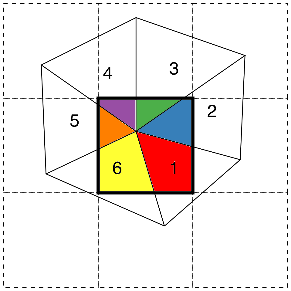
Figure 3 An illustrative example of how the conservative remapping algorithm works. In this case, the donor mesh consists of triangles, while the receiver mesh consists of quadrilaterals. The algorithm calculates the area of overlap for each triangle, starting in the triangle labelled 1, proceeding to no. 2, etc.

After adding N^′ to 𝒫₆, the program proceeds to perform checks two and three on element 6. Check two finds the corner point of the quadrilateral that lies in element 6, since N(ℰ_r)∈ℰ_d, and adds it to 𝒫₆. Check three finds the intersection points between the left-hand side of the quadrilateral and the side shared by elements 5 and 6, and between the bottom and the side shared by elements 6 and 1, as $X({\mathcal{E}}_{\mathrm{d},\mathrm{6}},{\mathcal{E}}_{\mathrm{r}})$. These are also added to 𝒫₆. As the I(ℰ_d,1) and I(ℰ_d,5) are already in ℒ, no recursive calls are made. The program then calculates the area of the yellow polygon in the figure, as A(𝒫₆) and adds this to the list 𝒲, and returns to the recursive call on element 5.

In element 5, the program completes the tests and computes the area of the orange polygon shown in the figure. No recursion is made, since all element numbers are already in ℒ. The program then exits to the recursive call on element 4, where the area of the purple polygon is computed, and so on. This procedure returns the list 𝒲 of the area of all the contributing polygons (coloured in the figure), as well as the list ℒ of the corresponding element numbers. These lists allow the program to calculate the weighted average contribution of the triangular elements to the resulting value in the quadrilateral. Once the lists ℒ and 𝒲 exist for all the receiver elements, the reverse contribution can be calculated as well.

5.3 OASIS coupling

NeXtSIM can be coupled to both ocean and wave models through the OASIS coupler (e.g. Boutin et al., 2021, 2023). OASIS (Craig et al., 2017) is a coupler that requires minimal code modification in the models being coupled and is very well suited to coupling substantially different code bases, as is the case here. To couple different models, each model must implement initialisation and finalisation routines and include the OASIS |get| and |put| function calls to receive and send coupling fields.

The OASIS interface implementation in neXtSIM is unusual because of the moving mesh neXtSIM uses. OASIS is designed for fixed meshes, and the OASIS initialisation routine should specify the mesh shape, coordinates, and domain decomposition. This allows OASIS to calculate interpolation weights and the communication pathways between the MPI domains of the different models once at startup. In the case of neXtSIM, the mesh and domain decomposition changes continuously throughout the simulation. Therefore, the OASIS interface in neXtSIM is set up so that the two models communicate through a fixed exchange grid within neXtSIM and on neXtSIM's root MPI processor.

For most setups, the exchange grid is identical to the grid of the other (ocean or wave) model. When coupling to an ocean model, the ice and ocean models must share an identical coastline to ensure the conservation of fluxes between them. The initial mesh of neXtSIM is then constructed to exactly trace the coastal boundaries of the exchange and ocean grid. NeXtSIM then uses the conservative remapping algorithm (Sect. 5.2) to interpolate between the moving mesh and the fixed exchange grid. To avoid recalculating the exchange weights at every time step (as in Sect. 5.2), the mesh is assumed stationary between remeshing steps.

The coupling procedure described above relies on several compromises in terms of both efficiency and accuracy. Recalculating the interpolation weights each time remeshing occurs is clearly less efficient than computing them only at the start of the run. The remapping algorithm we use is, however, efficient enough that this only takes about 5 % of the run time in a typical ice–ocean coupled setup (such as the one used by Boutin et al., 2023). Another efficiency loss arises because all communication must pass through the neXtSIM root MPI processor. It is difficult to assess this cost, but implementing proper parallel coupling was a significant step forward in the development of OASIS (Craig et al., 2017). In a typical ice–ocean setup, about 12 % of the total runtime is spent in the OASIS |put| and |get| routines, but this includes the time neXtSIM spends waiting for the ocean model. Some loss of accuracy occurs because the mesh is assumed to remain stationary between remeshing steps, but this has no greater impact on the solution than numerical noise inside the model itself (discussed in Korosov et al., 2023). In setups with resolutions between 10 and 20 km (e.g. Ólason et al., 2022; Boutin et al., 2023), remeshing occurs at three to six hourly intervals, resulting in displacement errors no larger than approximately 1/3 of the model resolution.

5.4 Input/output operations

NeXtSIM supports two output formats: snapshots of the model state with complete mesh information on the one hand, and netCDF output on a fixed, rectangular output grid on the other. The first is used to output the exact model state and is also used for restart files. The second is used to generate temporal averages and to simplify post-processing and analysis, as it is the standard format used in oceanography and climate science. The mesh-based snapshots are binary files of mesh and model field values, accompanied by ASCII files with the file header information. We have developed a library of Python routines called pynextsim (https://github.com/nansencenter/nextsim-tools, last access: 15 July 2026) to read, analyse, and modify the mesh-based output from neXtSIM.

In its simplest incarnation, the neXtSIM netCDF output uses a nearest-neighbour interpolation from the neXtSIM mesh to the output grid specified for the netCDF file. At each time step, the output field values in the element covering the centre point of each output grid cell are added to that grid cell's value, and the average is then written to file at the given output interval. Finding the overlap between the model mesh and the output grid is time-consuming, so we assume the mesh is stationary between remeshing steps. This is the same approach as in the coupling code, which is based on the same underlying functions as the netCDF output code.

The common code base for the coupling functions and netCDF output functions enables us to use the conservative remapping capabilities developed for coupling and remeshing. When in coupled mode, the netCDF output grid is the same as the coupler exchange grid and instead of using a nearest-neighbour interpolation, the conservative remapping approach is used. This has the added benefit that the netCDF outputs are conserving, which is crucial for budget calculations (e.g. Ólason et al., 2021; Boutin et al., 2023). This capacity can also be used in stand-alone mode, provided a specially crafted initial mesh and output grid definitions are provided, following the same requirements as for the mesh and exchange grid in the coupled case.

6 Simulation examples and use-cases

This section gives an overview of the model results and capabilities.

6.1 An idealised test case

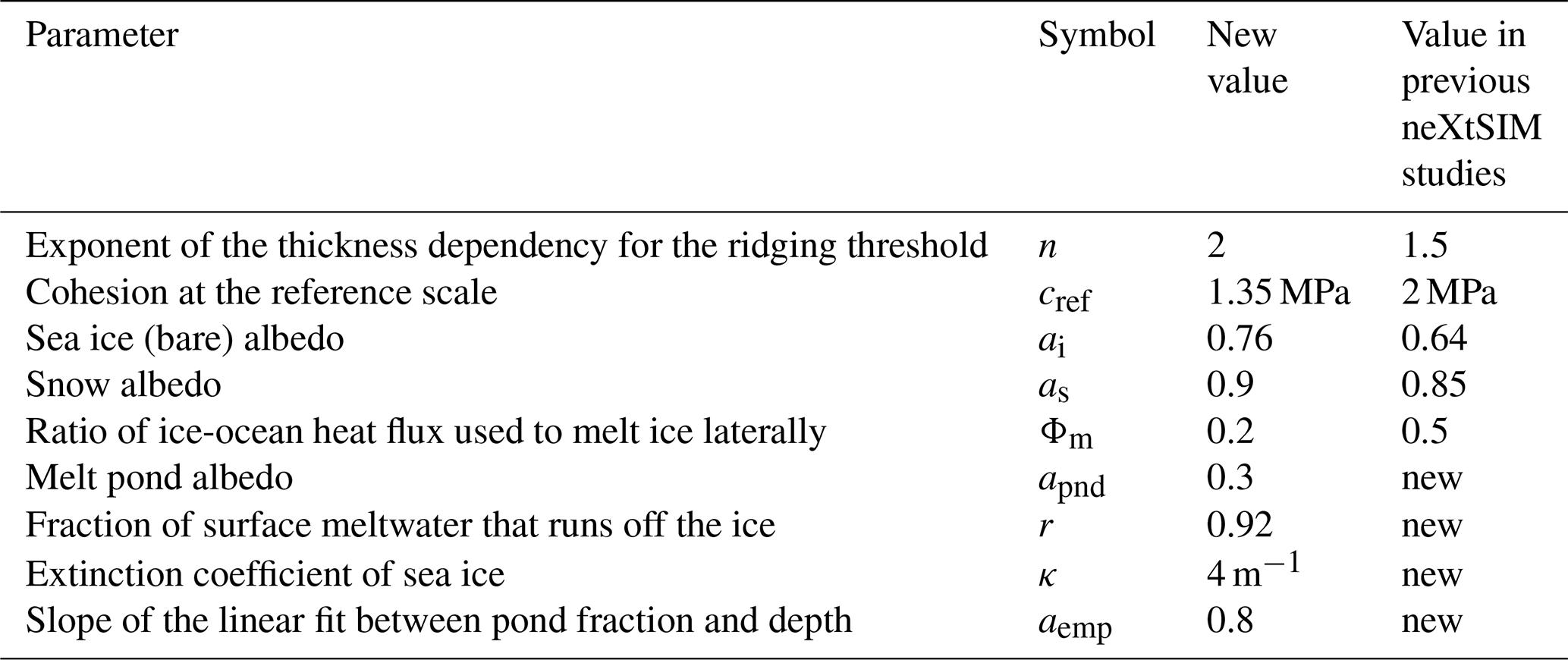
While neXtSIM was developed primarily to run large-scale simulations, the model can also be set up for idealised simulations to explore the details of certain physical processes and their parameterisations. To illustrate this, we show the results of an idealised experiment, exploring the difference between two damage update schemes. The two experiments consist of simulating a 1000×1000 km ice block fixed on one side to a coast with ice thickness 1 m, concentration 100 %, damage 0, and wind 5 m s⁻¹ blowing towards the coast (see Fig. 4a). The domain is located with the geographic North Pole at its lower left corner, resulting in a clear deviation of velocities due to the Coriolis effect. Both experiments run 24 h on a mesh with ≈10 km resolution, at 5 s time step, with 3 sub-steps. We use a short time step and few sub-steps to enable high-frequency output and a close inspection of the processes involved. Other parameters are taken from Ólason et al. (2022) and Table 1. In one experiment, the stress and damage are updated using the formulation from Ólason et al. (2022) (i.e., with $\mathrm{\Delta }t/t_{\mathrm{d}}$), and in the second one, using Eq. (43).

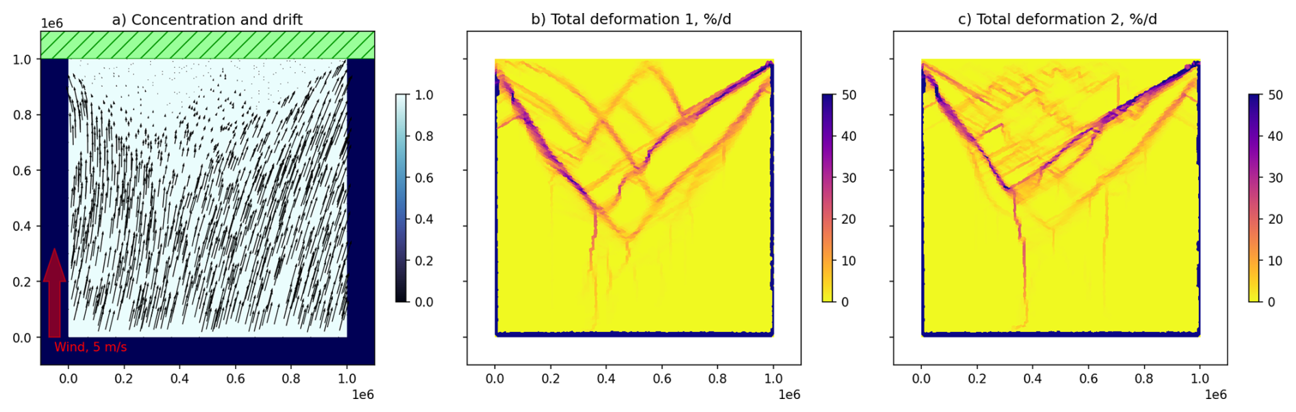
Figure 4 Drift and deformation after 24 h of model integration in an idealised experiment. The domain is 1000×1000 km with a constant wind of 5 m s⁻¹ blowing along the positive y-direction. Panel (a) shows the modelled concentration and drift, (b) the total deformation using the damaging scheme from Dansereau (2016) and Ólason et al. (2022), and (c) the total deformation using the damaging scheme in Eq. (43).

Table 1 Parameters used for the 15-year-long simulation in this study that differ from Ólason et al. (2022) (or earlier publications) or that are introduced in this study for the first time.

Of these two schemes, the latter ensures that the stress is always on or inside the failure envelope, while the former is derived from a differential equation for damage evolution. This differential equation is

$$\begin{array}{}\text{(113)}& {\displaystyle \frac{\partial d}{\partial t}}={\displaystyle \frac{\mathrm{1}-d_{\mathrm{crit}}}{t_{\mathrm{d}}}}(\mathrm{1}-d),\end{array}$$

where $t_{\mathrm{d}}=\frac{\mathrm{\Delta }x}{c_{\mathrm{E}}}$ is a characteristic time scale for damaging, based on the grid cell size, Δx and the propagation time of shear waves, c_E. An Euler-forward discretisation of this equation gives

$$\begin{array}{}\text{(114)}& d^{n+\mathrm{1}}=d^n+\left(\mathrm{1}-d_{\mathrm{crit}}\right)(\mathrm{1}-d){\displaystyle \frac{\mathrm{\Delta }t}{t_{\mathrm{d}}}}.\end{array}$$

In practice, the only difference between the two approaches is the factor $\mathrm{\Delta }t/t_{\mathrm{d}}$ which, because of the stability requirements of the explicit solver, must always be less than one. However, we can consider Eq. (43) to be a special case of Eq. (114) with $\mathrm{\Delta }t/t_{\mathrm{d}}=\mathrm{1}$ to force the stresses to always remain within the failure envelope.

Figure 4a shows the initial concentration and total ice motion over 24 h, while panels b and c show total deformation from the two experiments. Both deformation fields look somewhat similar; however, the results of the second experiment show narrower deformation zones and more small-scale faults in sea ice. To illustrate the differences in the process of ice faulting, we can analyse the propagation of the internal stress and damage in these experiments (see Fig. 5).

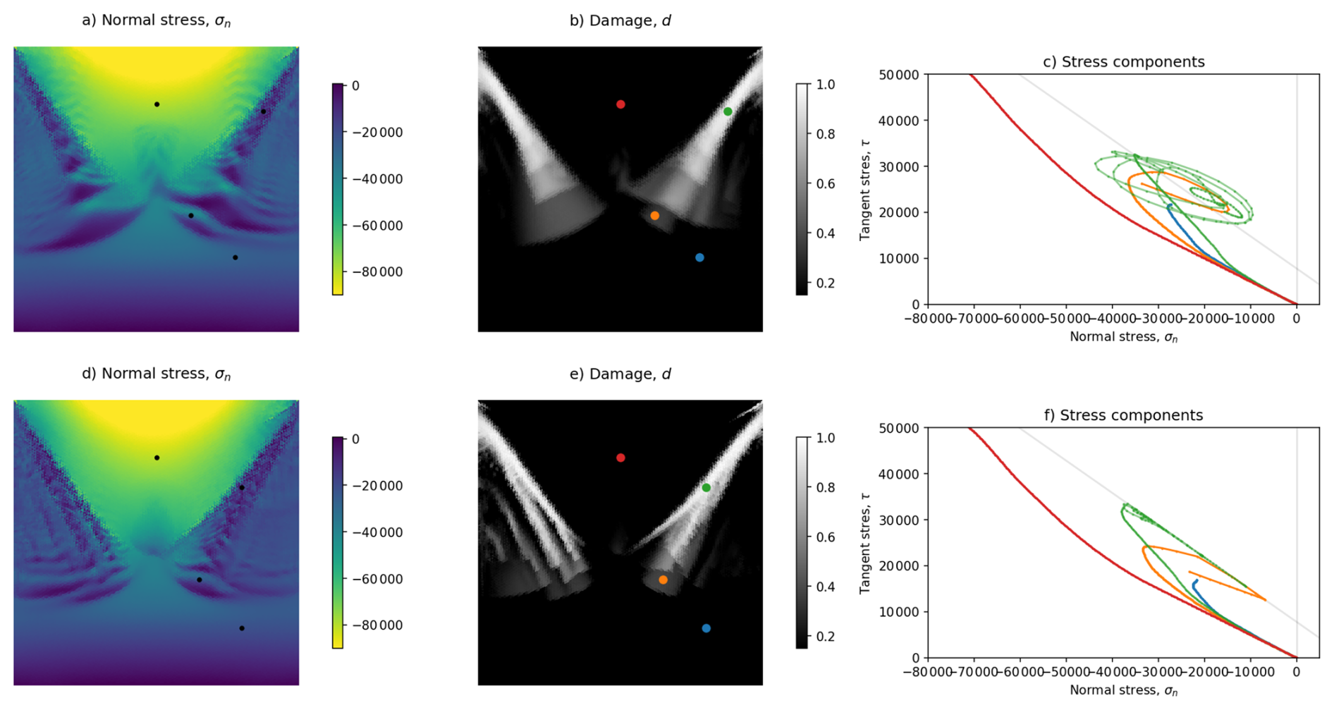
Figure 5 Normal stress, damage, and stress evolution at selected points of the domain using the two different damage and stress update schemes discussed in the text; with $\mathrm{\Delta }t/t_{\mathrm{d}}$ (a–c) and without $\mathrm{\Delta }t/t_{\mathrm{d}}$ (d–f). The fields are shown after 24 h of integration.

After 2 h, the fields of internal normal stress (σ_N, Fig. 5a and d) show quite similar patterns of two elastic wave trains propagating from the upper corners, where ice is attached to the coast and where the faulting started. Ice damage increases in the elements where the normal and shear stress exits the Mohr–Coulomb envelope, and lines of enhanced ice damage appear on the maps (Fig. 5b and e). On these maps, the main difference between the experiments is that the second one shows a narrower front of stress waves and, consequently, more localised damage. Analysis of the evolution of normal and shear stress (see Fig. 5c and f) can help explain this difference.

Two points (marked in blue and red in Fig. 5b and e) are located well outside the region of faulting, and the stress behaviour (shown by blue and red trajectories in Fig. 5c and f) is quite similar. Two other points (marked with orange and green dots) are located within the faulting zone. The orange dot experienced ice damage (and stress relaxation) only once, while the green one underwent several cycles of damage, stress relaxation, and stress build-up. Here, the stress trajectories differ significantly.

In the first experiment, the $\mathrm{\Delta }t/t_{\mathrm{d}}$ factor is always below one, and once the stress tensor of the element exits the fault envelope, the damage begins to increase slowly, and the stress begins to decrease slowly. Thus, the stress tensor returns to the envelope in more than one sub-step, manifested in a curved trajectory of normal/shear stress going outside the envelope for several steps and sub-steps (green line in Fig. 4c). At the same time, as stress is still relatively high and damage is not high enough, the stress starts to build up in the neighbouring elements, creating a broad front of the elastic wave. The broad front, in turn, leads to broader lines of increased damage.

In the second experiment, $\mathrm{\Delta }t/t_{\mathrm{d}}=\mathrm{1}$, the damage increases sufficiently quickly to allow the stress to return to the envelope in one sub-step. That pushes the stress tensor trajectory on the envelope, creating narrower elastic waves with higher damage localisation and small-scale background deformation lines. Such rapid change, however, tends to generate instabilities, leading to slightly noisier stress and damage fields. The way damage is modelled inevitably causes rapid, local changes in the stress state, which can promote noise in the stress and damage fields, as is visible in Fig. 4. This noise, however, does not appear to affect large-scale observable metrics, such as deformation statistics, considered in e.g. Rampal et al. (2016b) and Ólason et al. (2022). We therefore have not attempted to damp this noise. It is, however, interesting that the form of damage evolution affects the level of noise in the simulation. Further exploration of the origin, impact, and potential damping methods for this noise is left to future study.

These results demonstrate how using a dynamic timestep shorter than the damage propagation time, i.e. Δt<t_d, allows stresses in the model to temporarily exceed the failure envelope. This results in less localised damage and deformation fields. These supercritical states are short-lived but nonetheless affect the simulation results. Supercritical states are not physical but could be considered acceptable if the formulation improved model stability without significantly impacting the results. The numerical stability of the model in large-scale setups does, however, not appear to be affected by the formulation of Eqs. (43) and (45), even though the idealised tests do show increased instabilities when omitting $\mathrm{\Delta }t/t_{\mathrm{d}}$. The large-scale deformation in our 20 km resolution runs is also not affected to any substantial degree. In neXtSIM, we choose the formulation in Eqs. (43) and (45) to avoid the unphysical supercritical states.

6.2 Stand-alone 15-year simulation

As a large-scale sea ice model, neXtSIM's main goal is to represent the evolution of sea ice's large-scale properties most accurately, for time scales from a few days to decades. Here, we run a 15-year-long simulation of the model in a stand-alone configuration to illustrate the model's capacity to represent different aspects of sea ice properties in the context of a stand-alone simulation.

As in Ólason et al. (2022), we use the hourly ERA5 reanalysis (Hersbach et al., 2020) for atmospheric forcing and the TOPAZ4 reanalysis (Sakov et al., 2012) for oceanic forcing. Initial sea ice thickness and concentration are set from the PIOMAS reanalysis (Zhang and Rothrock, 2003). Initial sea ice damage is set to zero. We use the same domain as Ólason et al. (2022), but with a coarser horizontal resolution of 20 km (instead of 10 km). Key model parameters that differ from Ólason et al. (2022) or were introduced in this study are summarised in Table 1. We use a model time step of 1800 s and 120 sub-steps. The model was tuned to obtain reasonably good results in the observational comparison in the following sections. The tuning is based on the work of Williams et al. (2021), Ólason et al. (2022), Boutin et al. (2023), and Korosov et al. (2025).

To evaluate the consistency of neXtSIM's results, we compare them with various datasets of observed quantities. For sea ice extent, we use sea ice concentration from the climate data record of the EUMETSAT Ocean and Sea Ice Satellite Application Facility (OSI-SAF, Lavergne et al., 2019). For sea ice volume and thickness, we use the dataset combining the observations retrieved from the CryoSAT-2 and SMOS satellites, referred to as CS2SMOS (version 2.6, Ricker et al., 2017). For sea ice drift, we use the OSI-SAF climate data record (v1.0, Lavergne and Down, 2023). We use the dataset from the University of Bremen (Pohl et al., 2020; Istomina et al., 2025) retrieved using Sentinel-3 and ENVISAT for sea ice albedo and melt ponds. In our analysis, we generally compare model results and observations using the bias and RMSE. For sea ice extent, the bias is computed as described in Williams et al. (2021), and like them, we use the Integrated Ice Edge Error (IIEE, Goessling et al., 2016) instead of the RMSE as it provides more information about the model's capacity to capture the extent evolution. We use the same spatial domain for integrated quantities as Boutin et al. (2023), which includes most of the Arctic Ocean but excludes the Greenland Sea and seas south of Bering Strait. This is because we mainly focus on pack ice, for which neXtSIM was originally developed (Rampal et al., 2016a).

6.2.1 Extent and volume

Sea ice extent and volume are generally the first quantities to be evaluated due to their effect on climate. As shown in Ólason et al. (2022) and Boutin et al. (2023), neXtSIM can generally simulate their evolution in a way consistent with observations (Figs. 6 and 7).

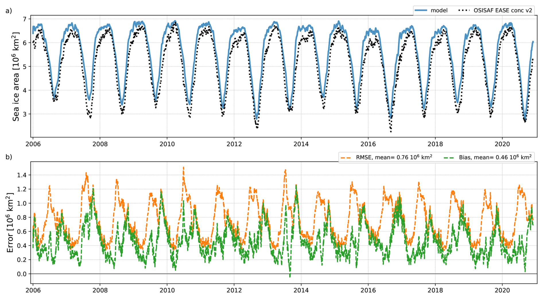
Figure 6 (a) Modelled and observed (OSI-SAF CDR) sea ice extent evolution for the period from January 2006 to December 2021. (b) IIEE and bias between the modelled sea ice drift and the OSI-SAF CDR dataset over the same period. The domain considered is shown in Fig. 7e.

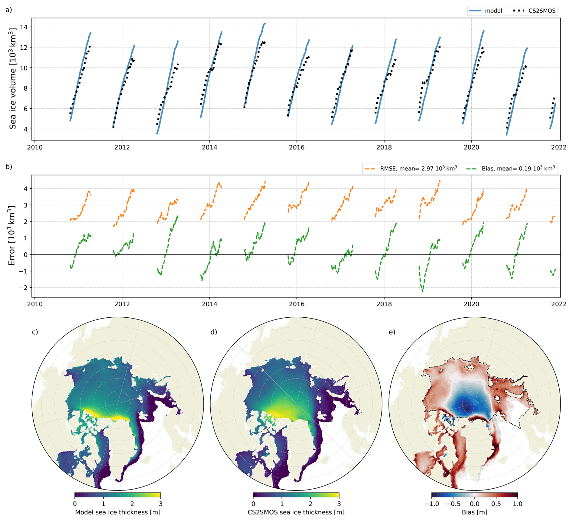
Figure 7 (a) Modelled and observed (CS2SMOS) sea ice extent evolution for the period from January 2006 to December 2021. (b) RMSE and bias between the modelled sea ice drift and the CS2SMOS dataset over the same period. (c, d) show the 2010–2021 November to April sea ice thickness climatology in the model and as estimated by CS2SMOS. (e) is the climatology of the sea ice thickness bias between the model and CS2SMOS. These climatologies are computed from monthly averaged files. The black dashed contour in (e) shows the domain used to compute integrated quantities in Sect. 6.2 (e.g., in panels a, b here).

As in the ice-ocean coupled setup presented in Boutin et al. (2023), sea ice extent is generally consistently captured (Fig. 6). IIEE peaks at the end of summer, when sea ice extent is minimal, but remains generally under 1 M km². It is associated with a positive bias, meaning the simulation overestimates the yearly minimum extent. IIEE is lower in winter, as most of the domain used for its computation is covered by stopped ice. As in Boutin et al. (2023), including the totality of the domain has little qualitative effect on the IIEE evolution.

Modelled sea ice thickness also shows reasonable agreement with data from CS2SMOS (Fig. 7). The interannual variability is visibly captured, and the slope corresponding to sea ice growth during the freezing season generally agrees with observations. The bias and RMSE both grow from autumn to the end of winter (Fig. 7b). In all years but 2011, the simulation first underestimated the amount of ice left at the end of the summer but then ended up growing more ice than in observations by April, when observations stopped being available. Looking at the thickness distribution, the general spatial patterns are captured, with thicker ice north of Greenland where the oldest ice is expected to be found (Fig. 7c and d), and thinner ice in areas generally covered by first-year ice. The difference in sea ice thickness distribution reflects the behaviour of bias and RMSE (Fig. 7e), with the thickness of older and thicker ice underestimated while the thickness of younger and thinner ice is overestimated. This is a typical bias of sea ice models (Watts et al., 2021), and results can be improved by tuning some parameters, like the albedo, that are not very constrained and have a large impact on the amount of ice surviving the summer. Thinner ice thickness is more sensitive to parameters like the maximum thickness of the young ice class.

6.2.2 Drift

Sea ice drift is also an important metric to assess the quality of a sea ice model, as it significantly impacts sea ice balance through its transport of sea ice and its export through the Fram Strait (in the Arctic). A good representation of sea ice drift also improves the sea ice thickness distribution by properly capturing the location of older and thicker ice (Regan et al., 2023).

The simulation shows an agreement comparable to previous studies using neXtSIM (Rampal et al., 2016b; Williams et al., 2021; Boutin et al., 2023), with a generally low RMSE (less than 4 km d⁻¹ most of the year, Fig. 8). Both short-term (a few days) and long-term (seasonal and interannual) variabilities are captured. The bias with the OSI-SAF CDR dataset shows a seasonal cycle as it increases in the summer. However, satellite-derived observations are not available in the summer. Instead, the OSI-SAF CDR uses estimates from a free-drift model with high uncertainties. Lavergne and Down (2023) suggest these estimates may be biased low, meaning it is uncertain whether our simulation is biased in the summer or not.

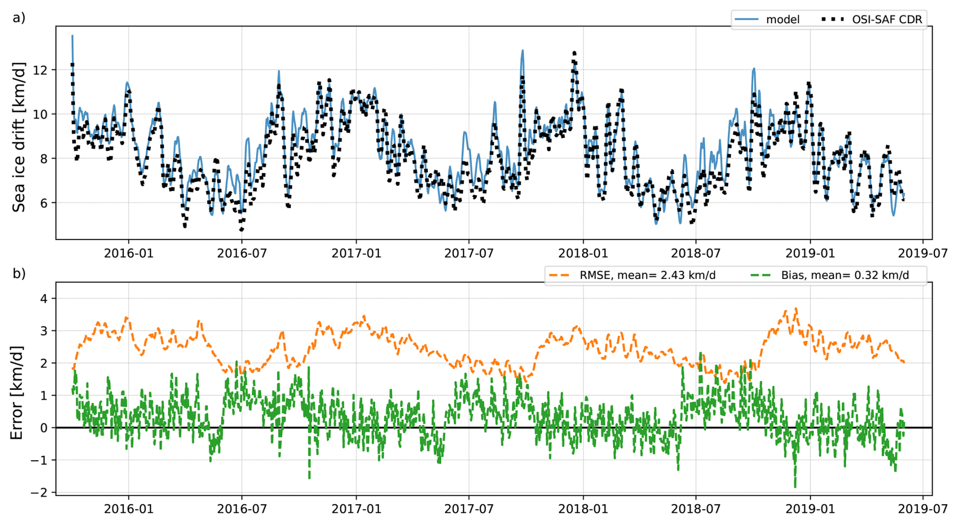
Figure 8 (a) Modelled and observed (OSI-SAF CDR) sea ice drift evolution for the period from October 2015 to June 2019. (b) RMSE (of drift speed) and bias between the modelled sea ice drift and the OSI-SAF CDR dataset over the same period. The domain considered is shown in Fig. 7e.

The mean Arctic-wide drift field also compares well with the OSI-SAF CDR dataset, showing a clear Beaufort Gyre circulation and a Trans-Polar Drift (Fig. 9). The modelled drift direction is generally very good, but the drift speed in the marginal seas teands to be too slow, while the drift in the central pack is too fast. The reason for this is difficult to pinpoint, especially since these are the results of a stand-alone model, without an active ocean model beneath. Lacking an active ocean will likely dampen the ice's drift speed.

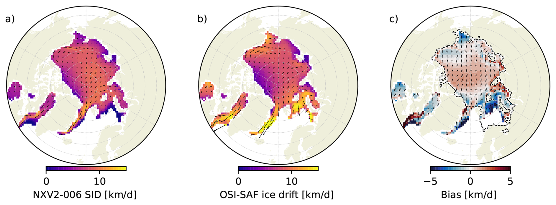
Figure 9 (a) Modelled and (b) observed (OSI-SAF CDR) sea ice drift for the period from October to June, over 2015–2019. (c) The model bias compared to observations, with colours showing the bias in speed and arrows bias in direction. Arrows pointing up indicate no directional bias.

The simulations used here do not use the stability-dependent drag coefficients introduced in Sect. 4.2. This is because taking atmospheric stability into account slightly increases the bias and RMSE between the modelled sea-ice drift and the OSI-SAF CDR dataset. We have been unable to determine why improving the physical representation in the model in this way gives worse results than the simpler approach of only using neutral drag coefficients. This issue will be investigated further in the near future.

6.2.3 Stress and damage

The BBM rheology in neXtSIM differs from VP and its derivatives in both the calculation of stress and the additional damage variable. No direct observations of these variables exist to compare with the model fields, but it is still instructive to present an example here. In this case, showing a snapshot from a single time step is more informative than showing long-term means, since averaging smooths out any features of interest. Figure 10a shows the modelled normal stress. We note that this is negative almost everywhere, indicating compressive stress, but that bands of high and low compressive stress are also visible in the field. These bands can also be seen in the shear stress field (Fig. 10b), indicating that the stress is concentrated along bands of shear failure. This feature is also visible in the damage field (Fig. 10c), which also shows similar striping. It is interesting to note that there is no direct correspondence between high stress and high damage, as the stresses respond to both the damage field and atmospheric and oceanic forcing. Finally, we note several isolated places along the coast where the normal stress is positive, indicating the presence of land-fast ice.

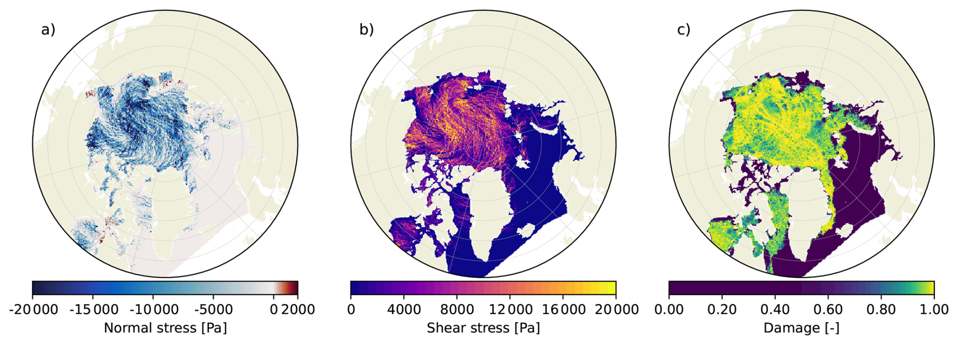
Figure 10 Modelled (a) normal stress, (b) shear stress, and (c) damage snapshots on the first time step of 3 March 2008.

6.2.4 Ridge ratio compared to observed sea-ice roughness

We compared the neXtSIM ridged ice thickness (computed as a product of ice thickness and ridged ice ratio) with ridging intensity from IceSat-2 (calculated as the ridge frequency per 1 km segment multiplied by the mean ridge sail height within the segment, Farrell et al., 2020). The maps in Fig. 11 show remarkable similarity in depicting high roughness in perennial ice and coastal areas with first-year ice, with very low ice roughness in the Central Arctic. The correlation between the neXtSIM ridged ice volume and the IceSat-2 ridging intensity is also high (0.617, Fig. 11), while correlations of other neXtSIM and IceSAT2 products are lower (see Table 2). The neXtSIM results also demonstrate how the model reproduces the strong heterogeneity that characterises sea–ice dynamics (e.g. Rampal et al., 2008).

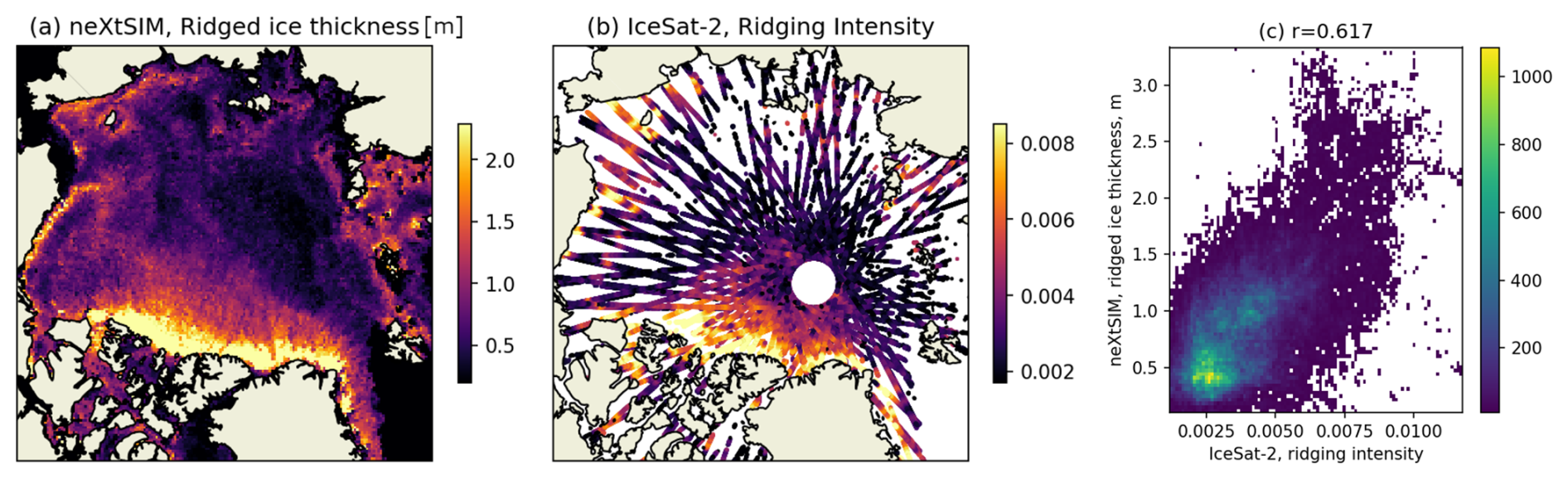
Figure 11 (a) Ridged ice thickness from neXtSIM on 4 April 2019, 12:00:00 LT. (b) Ridging intensity from IceSat-2 orbits acquired between 1 and 7 April 2019. (c) Scatter plot of IceSat-2 and neXtSIM products.

Table 2 Pearson's correlation between neXtSIM and IceSat-2 roughness-related products (significant at p<0.05 for all values). The correlation is highest between the IS2 ridging intensity and the modelled ridge ice thickness (in bold).

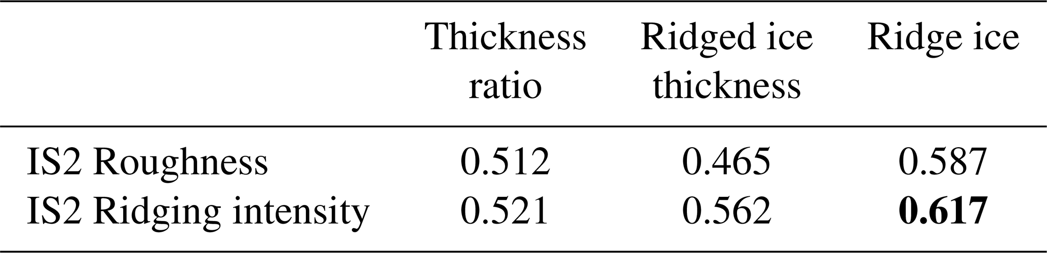
6.2.5 Melt-pond fraction compared to satellite observations

This paper introduced the newly implemented melt pond scheme in neXtSIM and its effect on albedo in Sect. 4.3. Here, we illustrate the behaviour of this scheme by comparing the seasonal distribution of the simulated sea ice albedo with estimates from the University of Bremen (Fig. 12). We notice that both the magnitude and the distribution of albedo are generally captured. This distribution is characterised by lower albedo at the margins of the sea ice cover and higher in the pack, with a strong latitude dependency in the observation dataset (see June in particular). The simulated albedo follows a general tendency but with a lower contract between pack ice and the ice edge and a generally lower albedo. This is partly explained when we look at the melt pond fraction (MPF) distribution (Fig. 13). This distribution differs between observations and the simulation. Observed melt pond fraction shows large values close to the sea ice edge and lower values in the interior, while July and August simulated MPF distributions are relatively uniform. We also notice that the modelled MPF is biased low in May–June but biased high later in August and September.

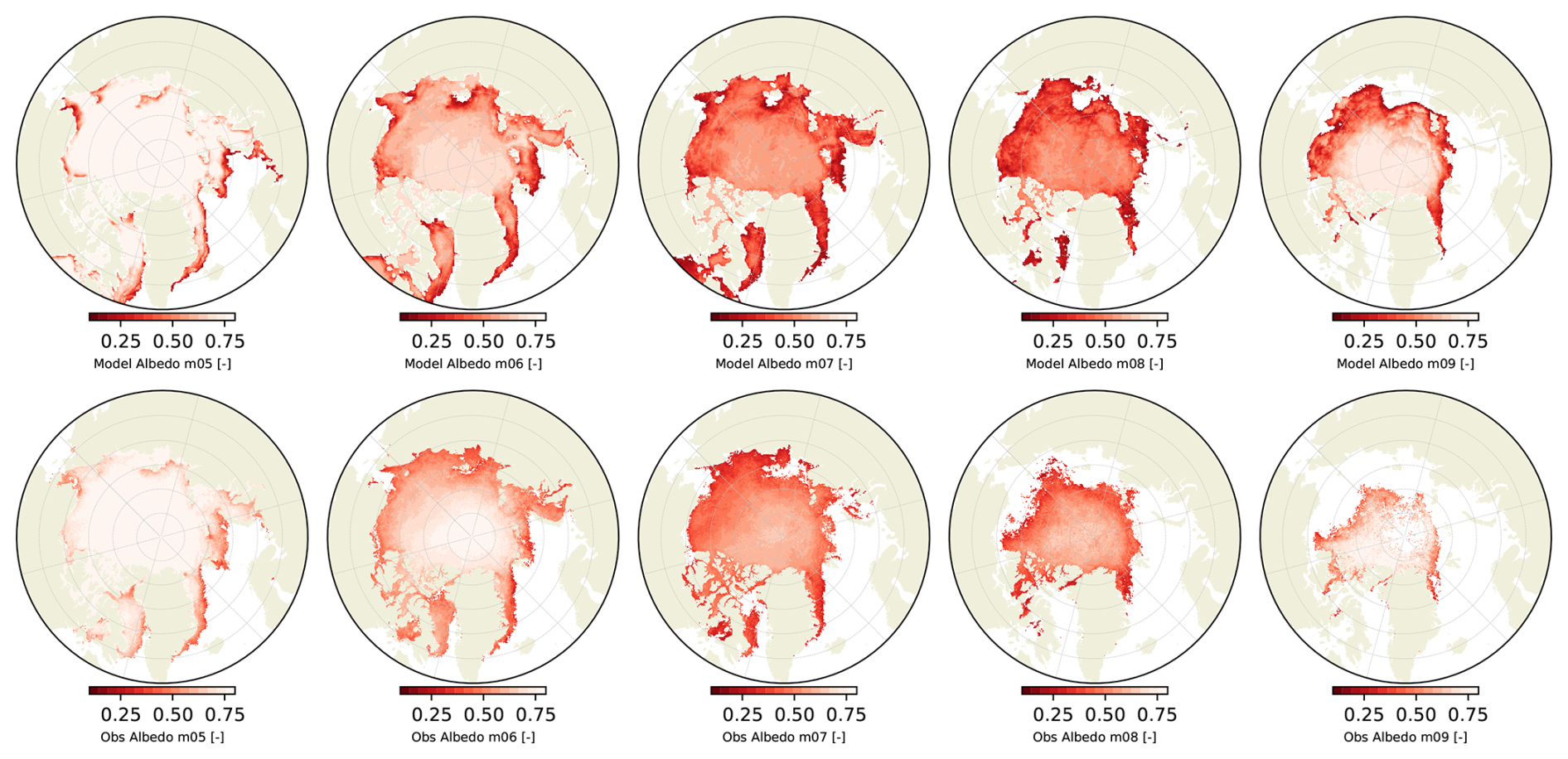
Figure 12 2017–2021 climatology of the simulated and the observed broadband albedo for the months from May to September, when the observation product from the University of Bremen is available.

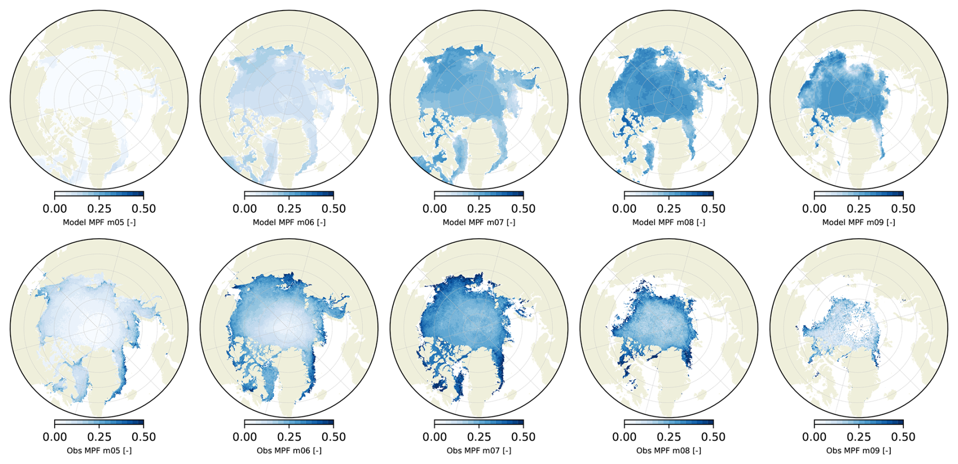
Figure 13 2017–2021 climatology of the simulated and the observed melt pond fractions for the months from May to September, when the observation product from the University of Bremen is available.

This behaviour of the MPF in the simulation can be explained mainly by simplifications we made in the parameterisation. The main simplifications are the absence of draining and the choice of a constant ratio of melted freshwater ending up in the ponds. Smith et al. (2025) suggest that this ratio is high early in the melt season (up to ≃40 %) and lower later (down to ≃10 %). In the absence of draining, using a higher ratio would result in largely overestimated MPF by the end of summer, and the choice of a constant ratio has the advantage of simplicity. Adding a dependency on concentration, as in, e.g., Holland et al. (2012), who assume lower concentrations have a lower ratio due to higher draining, would only increase the current biases by increasing MPF in the pack and reducing it in the margins. In reality, sea ice topography, roughness, and porosity must play a significant role in both this ratio and the amount of draining, but these dependencies are not yet fully understood. Nevertheless, activating the melt pond scheme albedo generally increases the sensitivity of simulated sea ice to melt (not shown), which helps reduce the extent of bias at the end of the summer. Still, it reduces the thickness of older ice, increasing the thickness bias we mentioned earlier. This effect is probably exacerbated by refrozen meltwater not counting towards ice mass in the model.

7 Interest of using neXtSIM

In this manuscript, we present the neXtSIM model and demonstrate its ability to simulate sea ice dynamics across a range of spatial and temporal scales. Here, we discuss the main advantages of using neXtSIM and its BBM rheology, as well as some of the current limitations.

Regarding computational performance, Ólason et al. (2022) found that the BBM rheology in neXtSIM is approximately 25 % slower than the mEVP rheology at a 10 km resolution, when using the same model time step and number of sub-cycles for the momentum equation solver. However, because BBM is a relatively new rheology in sea ice modelling, its computational efficiency has not yet been fully optimised. Ólason et al. (2022) also suggested parameter choices that could loosen the time-step requirements for BBM and make it faster than mEVP, highlighting its potential for further improvement.

The current version of neXtSIM faces two main computational limitations, both of which are already discussed in this manuscript. First, the remeshing procedure is not yet parallelised (see Sect. 5.1). Second, when neXtSIM is coupled with other models, the conservative remapping weights must be recomputed at regular intervals. Both limitations stem from the use of a moving mesh, which remains relatively uncommon in large-scale Earth system models. Ongoing developments aim to address these issues and have also motivated the implementation of the BBM rheology in Eulerian sea ice models such as SI3 (Brodeau et al., 2024).

From a sea ice modelling perspective, the main advantage of neXtSIM is its demonstrated ability to accurately reproduce small-scale deformation patterns, even at coarse spatial resolutions (Ólason et al., 2021, 2022; Bouchat et al., 2022; Hutter et al., 2022). This makes it particularly well-suited for investigating the role of small-scale deformations in sea ice evolution (Boutin et al., 2023; Rheinlænder et al., 2024) and their influence on other components of the Earth system, such as the ocean (Regan et al., 2025). Determining when, where, and to what extent these deformations are significant remains an open question – one that neXtSIM should be well equipped to explore.

8 Summary and conclusions

This paper presents the latest version of the next-generation sea-ice model, neXtSIM. It also marks the first open-source release of neXtSIM. This version depends on the core functionality already laid out in Rampal et al. (2016b), Samaké et al. (2017), and Ólason et al. (2022), but contains several significant new developments. The OASIS coupling interface and the associated conservative remapping algorithm are the most important technical developments. This was already used by Boutin et al. (2021, 2022, 2023) and Regan et al. (2023), but the technical details are described here for the first time. The ridge ratio and ice age tracers are also currently part of the Copernicus Marine Service's Arctic sea–ice forecast (https://doi.org/10.48670/moi-00004, Williams et al., 2021), but only described here in detail for the first time. The simulation results presented here also include more recent developments and physics implementations, such as the melt pond and atmospheric drag schemes, which have not yet been used in scientific publications or forecast products.