JCM v1.1: a differentiable, intermediate-complexity atmospheric model

In this paper we present version 1.1 of the JAX Circulation Model (JCM). JCM is a differentiable atmospheric model that is built in Python with the JAX numerical library and is released under a free and open-source software (FOSS) license. Earth system modeling is rapidly evolving, particularly through hybrid approaches that combine known dynamics with data-driven components. However, the training and validation of hybrid methods in traditional models remain difficult due to the absence of gradients and the complexity of legacy code. Differentiable models written in modern frameworks offer a path forward. JCM couples physics parameterizations to the Dinosaur dynamical core through a flexible interface that makes substitution of other schemes easy. The default parameterization scheme uses the SPEEDY (Simplified Parameterizations, primitivE-Equation DYnamics) intermediate-complexity physics scheme. This modularity supports benchmarking across physical and machine-learned schemes, with direct access to gradients for sensitivity analysis, calibration, and online learning. We show validation of JCM against the original Fortran SPEEDY code at T31 resolution. We also highlight JCM's differentiability and efficiency and outline plans for extending the framework to a differentiable Earth system model. JCM provides a lightweight yet expressive platform for accelerating research in climate modeling.

1 Introduction

Earth system models (ESMs) are critical tools for understanding and forecasting weather and climate, but the execution of these tasks is plagued by computational and scientific challenges (Shaw and Stevens, 2025). Predictions of the climate system are complicated by uncertainties in model architecture, initial and boundary conditions, and model parameters (Hawkins and Sutton, 2009). Furthermore, high-resolution or long-running global simulations are prohibitively expensive. Many strategies have been, and continue to be, developed to address some of these issues. For example, large ensembles can address uncertainty quantification (Kay et al., 2015; Rodgers et al., 2021; Eidhammer et al., 2024), hybrid models can leverage both data-driven and deterministic methods (Arcomano et al., 2020; Slater et al., 2023; Arcomano et al., 2023; Yu et al., 2023), and Bayesian inference can improve estimates of model parameters and forcings (Watson-Parris et al., 2021; Watson-Parris, 2025; Regayre et al., 2023). However, the development and intercomparison of these approaches in traditional climate models is hindered by complex legacy code, a lack of derivative information, and the inability to use modern hardware accelerators. Continued improvement of ESMs requires an upgrade in modeling infrastructure that takes advantage of state-of-the-art computational tools, particularly modern software frameworks (Gelbrecht et al., 2023).

Differential equations describe the evolution of dynamical systems and are common across a variety of disciplines. Gradients of these functions are relevant for analyzing input-output relationships, quantifying the influence of interactions between parameters, and assessing the robustness of results (Sapienza et al., 2025). In the case of ESM components such as atmosphere and ocean dynamics, ice flow, ecology, etc., the set of relevant differential equations is large and nonlinear. The analytical gradients of these functions are often unknown or are challenging to derive by hand. Automatic-differentiation (AD), also known as algorithmic-differentiation, uses software to compute the gradient of a function by systematically applying the chain rule. This technique has been in use for nearly 30 years but was historically tedious to implement (Giering and Kaminski, 1998). More recently, the explosion of machine learning (ML) applications has elevated the need for gradient information in order to train algorithms through back-propagation. This has led to the inclusion of AD in more accessible languages, such as Python, and has made differentiable programming a foundation of modern scientific computing (Blondel and Roulet, 2024). Differentiable software provides a common framework for Bayesian inference, inverse methods, optimization, and ML, leveraging decades of discovery from highly related fields of science and engineering (Sapienza et al., 2025).

One of the most promising uses of AD in geoscience is the online training of hybrid climate models (Rasp, 2020; Kochkov et al., 2024). Hybrid models combine ML components with traditional dynamical models. Data-driven components can support or replace existing physics parameterizations that are simplified and uncertain, with the hope that leveraging large amounts of data can improve model performance. The well-known equations that describe large-scale dynamics (i.e., a dynamical core) are left untouched. Popular candidates for data-driven parameterizations are atmospheric convection, cloud-aerosol interactions, and ocean turbulence. In theory, hybrid methods have the potential to benefit from the robustness of a deterministic dynamical core and the improved accuracy of ML-based parameterizations. In practice, the integration of ML components trained offline with dynamics is finicky and unstable (Rasp et al., 2018; Brenowitz and Bretherton, 2019). Differentiability allows for simultaneously tuning ML and physics-based parameterizations over multiple time steps, accounting for the online effects of coupling to a dynamical core. This can significantly improve the stability and accuracy of the resulting hybrid models. These benefits are exemplified by NeuralGCM, a hybrid atmospheric model that replaces the full physics-suite with a neural network (Kochkov et al., 2024) and by the recent study of Gelbrecht et al. (2025).

To evaluate the potential of hybrid climate modeling, there is a need for computationally efficient physics-based climate models with AD capabilities. Simplified chaotic models such as Lorenz 96 (Lorenz, 1995) do not provide a sufficiently complex test bed to meaningfully evaluate the merits of hybrid modeling (Rasp, 2020). NeuralGCM includes a realistic atmospheric dynamical core, but lacks physical parameterizations required for process-based understanding. Even without considering the availability of AD tools, running traditional climate models is computationally expensive. Fortran climate models were originally designed to run on CPUs and are extremely costly to port to state-of-the art processors. This is a fundamental limitation for their use in rapidly evolving climate modeling research with limited resources.

The JAX Circulation Model (JCM) is an intermediate-complexity atmospheric circulation model written in the Python programming language that takes advantage of the JAX library for hardware acceleration and differentiability (Bradbury et al., 2018). Python is the most commonly used programming language in the world, and its libraries are especially powerful for scientific analysis (e.g., Xarray and Dask) and ML (e.g., PyTorch and TensorFlow) (Hoyer et al., 2014; Dask Development Team, 2015; Paszke et al., 2016; Abadi et al., 2015). JAX is conveniently designed to use the familiar NumPy interface for array operations, while additionally providing efficiency and differentiability (NumPy Developers, 2006). Furthermore, programs written in Python and JAX can be deployed on central, graphics and tensor processing units (CPUs, GPUs and TPUs respectively) without modifications to the code. JCM takes advantage of these tools and thus is a user-friendly, differentiable model that is designed for hardware-acceleration and parallelism. Version 1.1 includes parameterizations for condensation, convection, radiation, and other atmospheric phenomena, yet is simplified compared to the most realistic models. JCM's modern software framework and representative physics schemes make it an ideal test bed for hybrid modeling and other AD applications. This work builds upon a growing movement to generate modular, differentiable Earth system components in modern programming languages with GPU acceleration (Klöwer et al., 2024; Häfner et al., 2018; Fang et al., 2024; Wagner et al., 2025).

This paper documents the version 1.1 release of the open-source JCM software and is organized as follows. Section 2 describes the model architecture and Sect. 3 shows examples of the model interface. Model validation and performance are discussed in Sects. 4 and 5. Section 6 discusses the use of AD in JCM in detail, including example applications. Finally, a summary and description of future directions is included in Sect. 7.

2 Model Architecture

JCM consists of a spectral dynamical core (dycore) and a suite of default physics parameterizations. The physics parameterizations are designed to be modular and easily swappable for future additions (e.g., replaceable by other physical parameterizations, prescribed forcings, or ML models). This section describes the dycore (dynamics), default physics parameterizations (physics), and the architectural choices that define version 1.1.

2.1 Dynamical core

JCM's dynamical core is called Dinosaur and was developed for use in NeuralGCM (Kochkov et al., 2024). The Dinosaur dycore is spectral and uses sigma levels (surfaces at fixed fractions of the surface pressure) for the vertical coordinate. It integrates the hydrostatic equations with a semi-implicit gravity wave scheme in addition to specified physics “terms” (see Sect. 2.2). The dycore's prognostic variables include horizontal wind (vorticity and divergence), temperature (anomaly from a reference temperature), and log surface pressure. Additional prognostic variables can be specified as tracers. In the default configuration of JCM, the only additional tracer is specific humidity. Dinosaur supports a range of horizontal grid resolutions; these are labeled by their spectral truncation, the maximum wavenumber of spherical harmonic they can resolve. Dinosaur's grids use a quadratic truncation, meaning there are 3 grid points per wavelength for the highest resolved wavenumber.

Supported spectral truncations range from T21 (a 64×32 grid) to T425 (a 1280×640 grid), with JCM's default being T31 (96×48, roughly 4°×4° grid cell size at the equator). There are no technical obstacles to adding support for resolutions beyond T425, though other features may be of higher priority for high-resolution studies, such as support for more vertical levels or for a non-spectral dynamical core. (Spectral integration schemes must simulate the entire globe, making them inefficient for region-focused experiments, and the spectral transforms required at each timestep eventually bottleneck performance as they scale worse than linearly with the number of grid points.) Dinosaur is capable of operating with many vertical levels. In JCM we use the 8σ levels expected by the default physics suite (described below). Sigma layer boundaries are at σ values of 0, 0.05, 0.14, 0.26, 0.42, 0.60, 0.77, 0.90 and 1. Prognostic variables other than log surface pressure are specified at the center of the sigma levels (σ=0.025, 0.095, 0.20, 0.34, 0.51, 0.685, 0.835, 0.95).

Time integration in JCM is performed with the IMEX (implicit-explicit) SIL3 (semi-implicit Lorenz three-cycle) Runge-Kutta scheme, which treats the linear terms of the primitive equations implicitly and the nonlinear advection and physics terms explicitly (Whitaker and Kar, 2013). IMEX SIL3 is second order accurate (discretization error scales with the square of the timestep) for the implicit terms and third order accurate for the explicit terms. The SPEEDY Fortran model uses a leapfrog scheme, but for simplicity we use IMEX SIL3, which does not require keeping track of state at multiple time-steps. The default time step is 30 min, although this can be easily varied at model initialization time. After computation of parameterized tendencies at each time step, horizontal diffusion of the prognostic variables is computed and the surface pressure field is corrected to maintain constant global mean surface pressure (mass conservation).

2.2 Physics parameterizations

JCM uses the physical parameterizations from SPEEDY (Simplified Parameterizations, primitivE-Equation DYnamics) version 41, which have been translated from Fortran90 to JAX. SPEEDY is an intermediate-complexity general circulation model developed at the International Centre for Theoretical Physics (ICTP) (Molteni, 2003). SPEEDY represents physical processes with simplified schemes that operate on 8 vertical levels. The top two layers represent the stratosphere, the bottom layer represents the planetary boundary layer, and the intermediate layers represent the free troposphere. SPEEDY has been used in a large number of studies, both on its own as well as in coupled contexts (with many different ocean models). Its lightweight design makes it an efficient sandbox for prototyping numerical schemes (Amezcua et al., 2011) or data assimilation methods (Sluka et al., 2016; Cintra and de Campos Velho, 2014; Ruiz and Pulido, 2015), looking at long-term climate interactions (Kucharski et al., 2006), or looking at the large-scale impacts of a wide range of climate forcings (Kucharski et al., 2013).

The SPEEDY parameterizations were developed by simplifying more complex physics schemes while retaining underlying physical principles. These simplifying assumptions are specifically intended to work for a model with few (order 10) vertical levels. Here we provide a brief overview of each of the SPEEDY physics parameterizations, and full details are available in the original model description paper (Kucharski and Molteni, 2013). The primary difference between the SPEEDY parameterizations and JCM is the handling of horizontal diffusion and orographic corrections, which is described in detail below. Neither SPEEDY nor JCM v1.1 implements a daily cycle.

• Convection. Convection is simulated with a simplified mass-flux scheme based on Tiedtke's 1989 paper (Tiedtke, 1989). Convection is activated in areas meeting two simultaneous criteria for conditional instability: humidity in the planetary boundary layer (the lowest layer) exceeding a prescribed threshold, and saturation moist static energy decreasing with height between the PBL and upper troposphere (the highest non-stratospheric layer). The cloud-base mass flux (at the top of the PBL) is calculated to relax the PBL humidity to its threshold value on a time scale of 6 h. The air in the updrafts is assumed to be saturated. Entrainment occurs in the lower half of the troposphere, and detrainment occurs only at the cloud-top level (determined by the conditional instability criterion).

• Large-Scale Condensation. Each sigma level has an associated threshold for relative humidity; when relative humidity exceeds this threshold, it is reduced back to the threshold value with a 4 h relaxation timescale, and the equivalent amount of latent heat is added to the dry static energy.

• Clouds. Non-stratocumulus cloud cover (and thickness) is diagnosed from the amount of precipitation and the free-tropospheric (excluding stratosphere and PBL layers) relative humidity profile in each air column. Stratocumulus clouds are diagnosed from the static stability in the PBL.

• Shortwave Radiation. SPEEDY represents shortwave radiation with a two-band radiation scheme, with one band for the near-IR part of the spectrum. The shortwave transmissivity of each model layer is computed as a function of layer mass, specific humidity, and cloud cover. Shortwave reflection occurs at cloud tops and at the surface.

• Longwave Radiation. SPEEDY's longwave radiation scheme has four spectral bands. One band represents the atmospheric “window”, while the other three bands represent the spectral regions of absorption by water vapor and carbon dioxide. Layer transmissivities are computed from layer mass and humidity, with cloud cover being represented as a decrease in “window” band transmissivity. At each layer, the downward longwave radiation flux is computed as a weighted function of air temperature at the full level and the interpolated air temperature at the half-level below. Upward flux is computed similarly, using the half-level above instead.

• Surface Fluxes of Momentum and Energy. Fluxes of momentum and energy from the surface to the atmosphere are computed using bulk aerodynamic formulas; one set of exchange coefficients is used over land and another set is used over ocean. For momentum flux, the land coefficient is a function of topographic height. For sensible and latent heat fluxes, the coefficients depend on a simple near-surface stability index based on surface energy balance. Evaporation is estimated using a scheme similar to that outlined in Viterbo and Beljaars (1995).

• Vertical Diffusion. SPEEDY's vertical diffusion module simulates three processes. First, shallow convection is simulated by mixing moisture and dry static energy between the lowest two model layers. Second, lower-troposphere diffusion of water vapor in stable conditions is estimated based on the column's humidity profile. Third, diffusion is computed for dry static energy in areas where air temperature approaches a dry-adiabatic lapse rate.

• Horizontal Diffusion. SPEEDY incorporates implicit horizontal diffusion filtering into its leap-frog time integration, in addition to utilizing a Robert-Asselin-Williams filter (Williams, 2011). As mentioned above, JCM does not use leap-frog and instead uses Runge-Kutta. The exact same horizontal diffusion implementation is therefore not appropriate. In Version 1.1, JCM instead implements explicit Laplacian horizontal diffusion of the prognostic state. The timescales and order of the filter vary across the elements of the state. Divergence is diffused at a timescale of two hours with filter order 2. A fourth order filter is applied to vorticity and specific humidity with a timescale of 12 h and to temperature with a timescale of 24 h. The longer timescales associated with vorticity, temperature, and humidity are intended to preserve strong gradients that are important to drive realistic atmospheric circulation. Tuning and improvement of this filtering scheme is subject to future work.

• Orographic Corrections. Speedy.f90 includes corrections to the temperature and humidity fields that are not described in the SPEEDY documentation. These corrections appear to adjust near-surface temperature and humidity profiles to account for subgrid-scale topography. Version 1.1 of the JCM does not yet implement these corrections, but their inclusion is a subject of future work. The absence of these corrections is one of the ways in which the JAX implementation deviates from the Fortran 90 version.

3 Model Interface (API)

JCM's documentation is available at https://jax-gcm.readthedocs.io (last access: 29 May 2026). A key feature of the model is the simple and intuitive user interface in Python. Users construct a jcm.Model object with their desired grid geometry (including orography), and desired suite of physics parameterizations (e.g. SPEEDY), then call Model.run, specifying run length, (optionally time-varying) forcing terms, and the frequency at which to save output. Users can also specify a custom initial state and land surface boundary conditions. Model.run returns a struct containing the values of the prognostic dynamics variables and diagnostic physics variables over the course of the run. The struct can effortlessly be converted to an Xarray dataset. Example code for running the model is shown in Fig. 1.

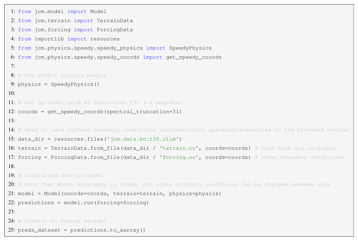
Figure 1 Running JCM with SPEEDY physics module and specified land surface boundary conditions, and converting the model output to an Xarray dataset.

4 Model Validation

In this section we provide validation of JCM against the version of the SPEEDY model implemented in speedy.f90 (Hatfield, 2022). We evaluate the prognostic state in addition to the global climatology of parameterized quantities such as cloud cover and precipitation.

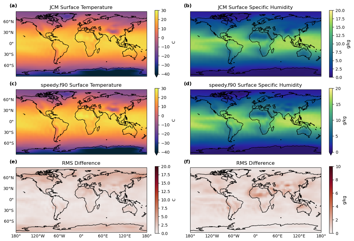
Figure 2 Average surface temperature and surface specific humidity in the surface layer in JCM (a, b) and in speedy.f90 (c, d). The root-mean-square (RMS) difference between the two simulations is shown in panels (e) and (f).

4.1 JCM versus SPEEDY

Both JCM and speedy.f90 simulations begin at isothermal rest and run for three years. The models are forced by a monthly climatology of sea-surface temperature, surface albedo, land surface temperature, soil moisture, sea ice concentration, and snow cover along with realistic orography. This monthly climatology is obtained from ERA-Interim over the period 1979–2008 (Dee et al., 2011). In addition to sharing initial and boundary conditions, both simulations are run at T31 resolution with a time step of 40 min. The first three months of the model runs are discarded as model “spin up”. Figures 2 through 5 validate the mean state of JCM against the mean state of speedy.f90. Figure 2 shows surface temperature and specific humidity in both models. The root-mean-square (RMS) difference of the 3-year simulations is shown in the bottom row. As mentioned in Sect. 2, JCM does not yet have orographic corrections. This leads to slight differences between the two models in temperature and specific humidity over land. The average RMS difference at the surface is 1.8 °C and 0.68 g kg⁻¹.

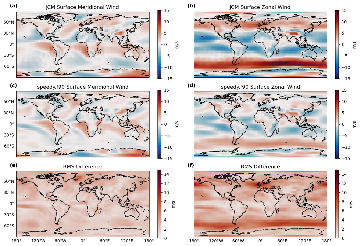
Figure 3 Average meridional and zonal winds in the surface layer in JCM (a, b) and in speedy.f90 (c, d). The RMS difference between the two simulations is shown in panels (e) and (f).

Figure 3 shows the average meridional (left) and zonal (right) wind in the surface layer. Again the RMS difference is shown in the bottom row. Large-scale patterns in meridional wind are the same between the two models with slight differences in strength, with JCM winds tending to be stronger than in speedy.f90. The zonal winds are generally stronger everywhere in JCM than in speedy.f90, and is most notable in the mid-latitudes. The discrepancy between the zonal wind in speedy.f90 and JCM is likely due to differences in the implementation of the time stepping and horizontal diffusion. The JCM parameterizations have been tested against speedy.f90 to verify that they produce the same output. This does not include horizontal diffusion, which in speedy.f90 is implemented implicitly in coordination with the leap frog time stepping. Although the general formulation of the spectral dynamical cores is the same, they are not identical and the additional choices to use Runge-Kutta and explicit horizontal diffusion in the JCM lead to differing results. Speedy.f90 also implements additional linear drag on the mean vorticity and divergence in the stratosphere (this drag is undocumented and thus currently excluded from the JCM). JCM v1.1 has been tuned to reduce these differences where possible. While we aim to match the qualitative climate of the Fortran, we are not prioritizing reproducing speedy.f90 exactly, and instead use it as a starting point for an intermediate-complexity model. These architectural choices are also described in Sect. 2. The average RMS difference of meridional and zonal winds at the surface are 2.1 and 3.5 m s⁻¹ respectively. Figure 4 shows a comparison of the winds at the top of the troposphere. Again, the large-scale patterns are qualitatively similar, but JCM winds are stronger than in speedy.f90. The average RMS difference of meridional winds at the top of the troposphere is similar to at the surface, but the average RMS difference in the zonal winds is roughly 9 m s⁻¹.

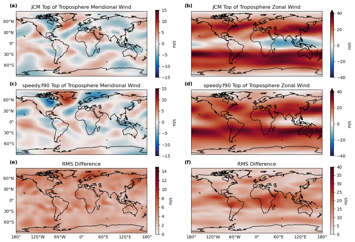
Figure 4 Average meridional and zonal winds at the top of the troposphere in JCM (a, b) and in speedy.f90 (c, d). The top of the troposphere, as defined by the SPEEDY model, is the third sigma layer from the top of the atmosphere. The RMS difference between the two simulations is shown in panels (e) and (f).

4.2 Cloud Cover and Precipitation

In addition to validating the prognostic JCM state against SPEEDY, we verify the spatial patterns of cloud cover and precipitation. Figure 5 shows average stratiform cloud cover fraction, precipitation due to convection, and precipitation due to large scale condensation. The panel (a) indicates that low clouds are most prevalent along the eastern boundaries of ocean basins in both JCM and speedy.f90, with average cloud cover near 40 %. This pattern agrees well with the climatology described by Hartmann (2016). Panels (b), (c), (e) and (f) show precipitation patterns associated with different physical processes. Convective precipitation (b and e) is highest in the tropics, and is particularly strong near the inter-tropical convergence zone (ITCZ), the Pacific warm pool, the Indian Ocean, and the equatorial Atlantic. While JCM and speedy.f90 show the same spatial patterns, precipitation due to convection is more concentrated in speedy.f90 and more diffuse in JCM, likely due to the larger spatial scales of the horizontal diffusion. Precipitation due to large-scale condensation (c and f) is highest in the mid-latitudes with hotspots over the North Pacific Ocean, the Gulf Stream, the Himalayas, and the Southern Ocean. Large-scale condensation appears to be slightly stronger in JCM than in speedy.f90. Spectral ringing in low-resolution models is a common phenomenon (Durran, 1999). Artifacts of this type of ringing can be seen in Fig. 5 in the results from both models. However, the ringing in JCM is stronger than in speedy.f90. We have investigated whether this difference affects model stability, and we have found no indication that it grows over time in these low-resolution configurations (T31-T85). This includes running the model for 100-year runs and taking gradients through those long integrations.

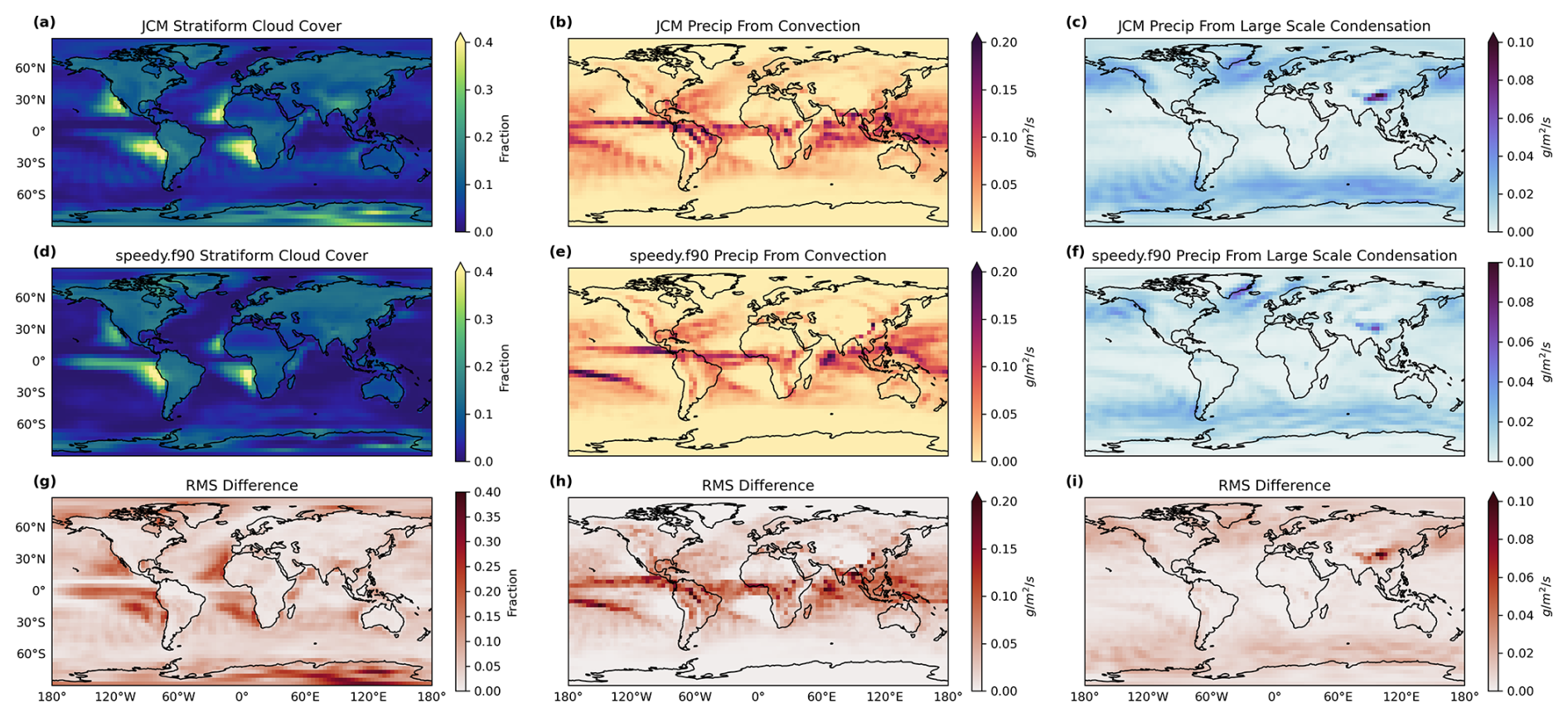
Figure 5 Average stratiform cloud cover (a, d), precipitation due to convection (b, e), and precipitation due to large scale condensation (c, f). RMS difference between JCM and speedy.f90 is shown in panels (g)–(i).

5 Performance

JCM is lightweight enough to be practical for running on even small-scale systems such as a personal laptop CPU. For higher grid resolutions, model runs longer than a few months of simulation time, or intensive gradient computations, JCM is best run with some form of hardware acceleration (i.e. on a GPU or TPU), which is natively supported through JAX. Figure 6 shows the simulation speed, in units of simulated years per day (SYPD), of running JCM at various resolutions and on various device types. The behavior in the figure has been our typical experience: runtime on GPUs and TPUs is significantly faster than on CPUs, with parallelization (sharding the model state arrays so they can be distributed among multiple devices) giving an additional significant speedup to TPU runs on Google Cloud (parallelization was not used for the results in Fig. 6). The dashed line in the figure represents the theoretical quadratic scaling of number of operations (and memory requirement) with spectral truncation.

Before a run is executed, there is a small amount of compilation time (10–15 s for typical runs at default resolution) which varies little with resolution and run length. Advanced users conducting many short runs with varying initial conditions or forcings should use jcm.Model.run_from_state, a slight variant of jcm.Model.run which after the first run with a given resolution, timestep, save interval and total time requires no compilation time for any subsequent runs with the same values for those parameters. We encourage users to read the JCM documentation for details.

Beyond basic vectorization of loops and conditionals in the code logic, no effort has yet been made to optimize JCM's performance on all platforms, especially for cloud computing at high resolution. As such, we expect there will be significant performance improvements in the future.

It should be noted that in practice, the runtime for the higher resolutions may pick up another factor of 2 or 3 relative to lower resolutions due to reductions to the model timestep that are eventually needed for stability. For the results shown in Fig. 6, the timestep was left as the default 30 min for all resolutions.

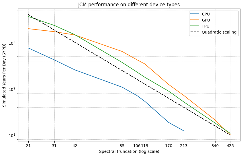
Figure 6 Model performance on different hardware for a default JCM run, 30 min timestep. To generate this plot, runs of 1 simulated year were conducted on 3 types of Google Cloud virtual machines: a CPU VM (with 32× Intel Xeon Platinum 8581C), a GPU VM (with a 16 GB Tesla P100 PCIe), and a TPU VM (with a Google Cloud TPU v5 lite). These devices were chosen as comparable based on having similar pricing (approx. USD 1.50 h⁻¹) at time of writing.

6 Gradients

One of the benefits of JAX is the accessibility of gradient information. JCM gradients can be taken with respect to inputs (e.g., initial conditions and forcing), outputs (e.g., the future model state), and parameters (e.g., SPEEDY physics parameters). In this section we explain and highlight use cases of these gradients including calibration and sensitivity analysis. The JAX library provides verification functions to test model gradients against finite difference estimates, which are included in the unit testing suite for JCM.

6.1 Automatic-differentiation (VJP and JVP)

Automatic differentiation (AD, also called algorithmic differentiation) computes derivatives of functions by recursively applying the chain rule to the computational graph. When AD is not available, tangent linear and adjoint models must be manually derived and implemented. Given the complexity of state-of-the-art Fortran models, this manual generation of gradients is expensive to implement and maintain. Thus, in most cases, gradient information is inaccessible or presents a substantial burden to model developers.

JAX provides JCM with its AD capabilities (Bradbury et al., 2018). In JAX, gradients can be computed in either forward (tangent linear) or reverse (adjoint) mode. Each mode has multiple use cases and can be applied to a wide variety of science problems. We use F(x) to denote the tangent linear model of a function ℱ(x) with input parameters x. The relationship of F(x) to the adjoint model F^T(x), where both are linearized about x, is

$$\begin{array}{}\text{(1)}& \langle F\left(x\right)\mathit{v},\mathit{w}\rangle =\langle \mathit{v},F^T\left(x\right)\mathit{w}\rangle ,\end{array}$$

where v is the tangent vector, w is the co-tangent vector, and 〈⋅〉 denotes the inner product. Forward-mode differentiation is applied through the Jacobian vector product (JVP) and is equivalent to F(x) v. This evaluates the multiplication of a user-specified tangent vector, v, with the tangent linear model, F(x). Reverse-mode differentiation evaluates a vector-Jacobian product (VJP), equivalent to F^T(x) w. This multiplies a user-specified co-tangent vector, w, with the AD-derived adjoint, F^T(x), of the function ℱ(x). Both VJP and JVP avoid computing the entire Jacobian of the function to minimize computational cost, but they can be used to reconstruct it if necessary. Example applications are discussed in more detail in the following sections.

In large-scale geophysical models integrated over long time windows, JVP typically costs approximately 1–2 times the cost of a nonlinear forward model integration. In contrast, VJP often costs approximately 3–6 times the cost of the forward integration, depending on memory constraints, checkpointing strategy, and solver structure (Heimbach et al., 2005; Evensen et al., 2020). Reverse-mode differentiation is more computationally efficient than forward mode for gradient evaluation when the output dimension of the function of interest is much smaller than the input dimension (e.g., a scalar loss function). In this case, a single VJP evaluation produces the full gradient, whereas forward mode would require n separate JVP evaluations, where n is the input dimension. Conversely, forward-mode differentiation is more efficient when the number of inputs is much smaller than the number of outputs.

6.2 Calibration

Calibration of ESMs against observations is a problem of interest to the geoscience community and benefits from gradient information. The goal of ESM calibration is to estimate physics parameters that generate the best match between a model trajectory and observations. Without gradient information, this process involves ensemble methods and hand-tuning by domain experts. Hand-tuning is limited in the degree to which it utilizes observational information and leaves much of the parameter space unexplored. Ensemble methods can be effective, but we often lack comparisons of these approximations against gradient-based approaches. Such comparisons are a focus for future work with the JCM. With gradient information, we can take a more systematic approach to calibration using gradient-based optimization techniques. Calibration with gradient information has the potential to assess model behaviour across more of the parameter space.

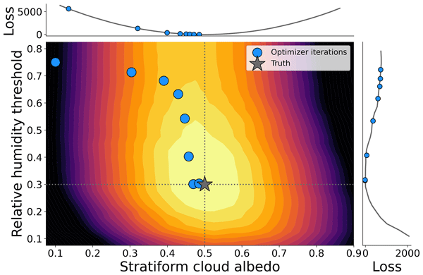
A popular approach for ESM calibration is to estimate model parameters against climate statistics (Kennedy and O'Hagan, 2001; Schneider et al., 2017, 2024). The optimization problem is formulated to minimize a loss defined by the misfit between observed and modeled statistics. In order to illustrate how JCM can be calibrated using AD, we show an idealized example that simultaneously estimates parameter values for stratiform cloud albedo and relative humidity threshold. We generate synthetic observed statistics by running the JCM in the default aquaplanet configuration, which has values of stratiform cloud albedo =0.5 and relative humidity threshold =0.3. The calculated statistics are the spatial and temporal averages of each model output variable over a 5 d model run. We initialize the starting values of stratiform cloud albedo and relative humidity threshold to be 0.1 and 0.75, respectively, and then optimize over the parameter space to find values that most closely reproduce the synthetic statistics. The observations denoted by y in Eq. (2) correspond to the simulated statistics. This example can be adapted or extended to use any climate statistics and any set of parameters.

In this example case, the function ℱ(⋅) is a 5 d JCM simulation with stratiform cloud albedo and relative humidity threshold = x. The loss function ℒ(⋅) is then defined as

$$\begin{array}{}\text{(2)}& \mathcal{L}\left(x\right)={\displaystyle \frac{\mathrm{1}}{\mathrm{2}}}{∥{\mathbf{R}}^{-\frac{\mathrm{1}}{\mathrm{2}}}y-\mathcal{F}\left(x\right)∥}_{\mathrm{2}}^{\mathrm{2}},\end{array}$$

where ∥⋅∥₂ defines the L-2 norm, and R is the observational covariance matrix. R is assumed to be a diagonal matrix with variances =1. We use a gradient descent optimizer to solve for the value of x that minimizes the loss. There are many other types of optimization algorithms, but given the low complexity and smooth loss landscape, we chose the simplest approach. The gradient descent update is as follows:

$$\begin{array}{}\text{(3)}& x_{k+\mathrm{1}}=x_k-\mathit{\alpha }\left({\displaystyle \frac{\partial \mathcal{L}}{\partial x_k}}\right),\end{array}$$

where x_k denotes the vector of parameter values at iteration k, α denotes the step size, and the search direction is the negative gradient of the loss with respect to x_k. Figure 7 shows the calculated loss at each step of the optimization (blue dots) and the true parameter values (grey star). It can be seen that the optimizer succeeds at identifying the values that generated the simulated observations. We calculate the loss across the possible range for both parameters and include a visualization of the 2-dimensional loss landscape, where light colors signify lower cost.

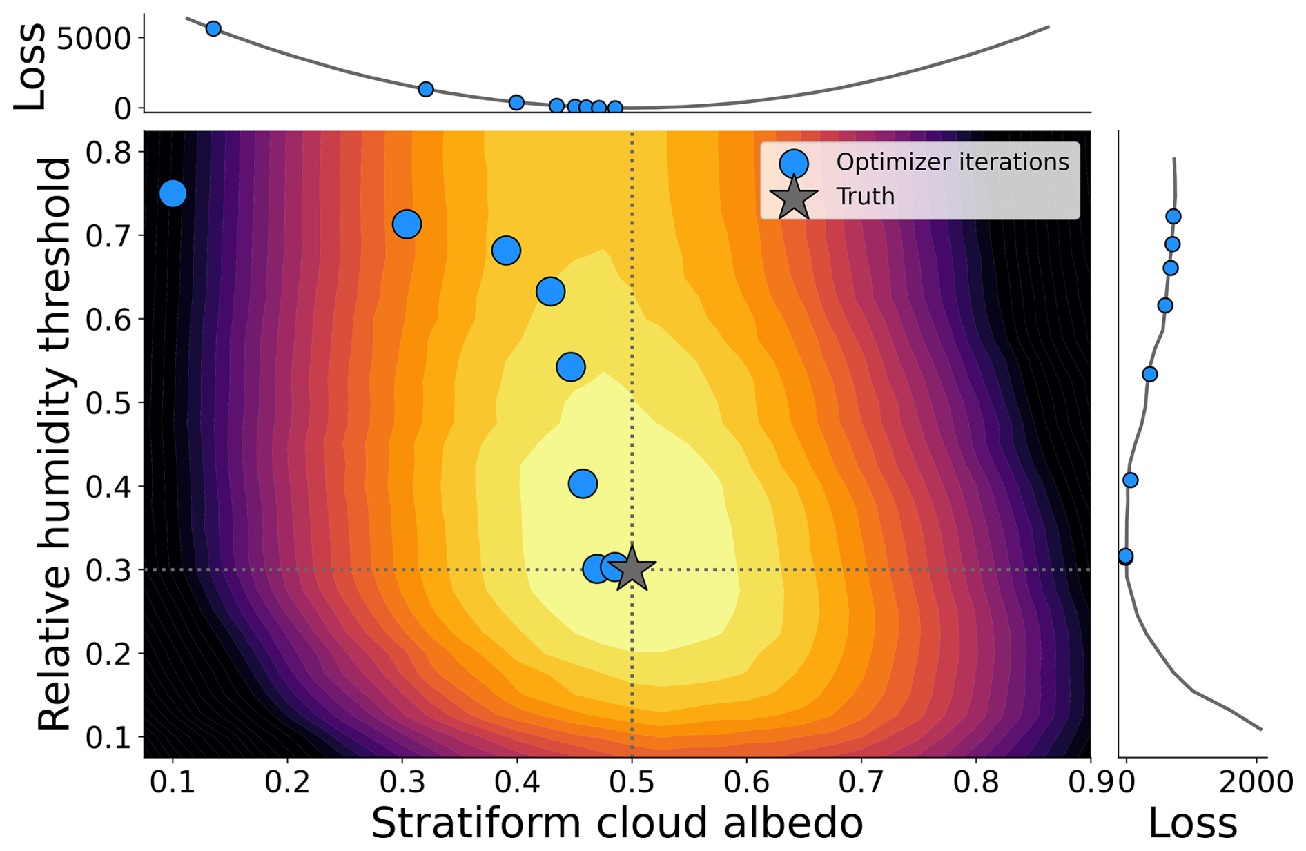
Figure 7 Visualisation of the 2-D loss landscape for the described parameter estimation example. The optimization begins with values of 0.1 for stratiform cloud albedo and 0.75 for relative humidity threshold. The optimal value is successfully found near the true SPEEDY values of 0.5 and 0.3, respectively. Blue dots show the calculated loss at each iteration of gradient descent, and the grey star is the “true” value. Curves at the top and right sides of the contour plot show slices of the loss function obtained by varying the parameters independently.

The gradient descent steps are plotted as blue dots to show the loss at each iteration. We obtain $\partial \mathcal{L}/\partial x_k$ using reverse mode automatic differentiation, providing the direction for the next parameter update. The gradient descent optimizer successfully identifies the value of stratiform cloud albedo used to generate the “true” statistics.

6.3 Sensitivity analysis

JVP facilitates sensitivity experiments with JCM. When using JVP, the tangent vector is effectively a perturbation that is propagated through the tangent linear model. If the function we differentiate is a JCM trajectory, then JVP gives us the evolution of an input perturbation to the model. This could be a perturbed parameter value, model forcing, or initial conditions. The model run is represented by ℱ(x), where argument x is the model input we will perturb. f denotes the model outputs of interest. Using forward mode automatic differentiation, we can calculate the change in the outputs, Δf, given perturbation Δx, which is approximated by

$$\begin{array}{}\text{(4)}& \mathrm{\Delta }f\approx F\left(x_{\mathrm{0}}\right)\mathrm{\Delta }x,\end{array}$$

where x₀ is the input to the model forward run and F(⋅) is the tangent linear model. JVP is used to evaluate the right-hand side of Eq. (4). The user only needs to provide the function ℱ(x) and the perturbation Δx (i.e., the tangent vector).

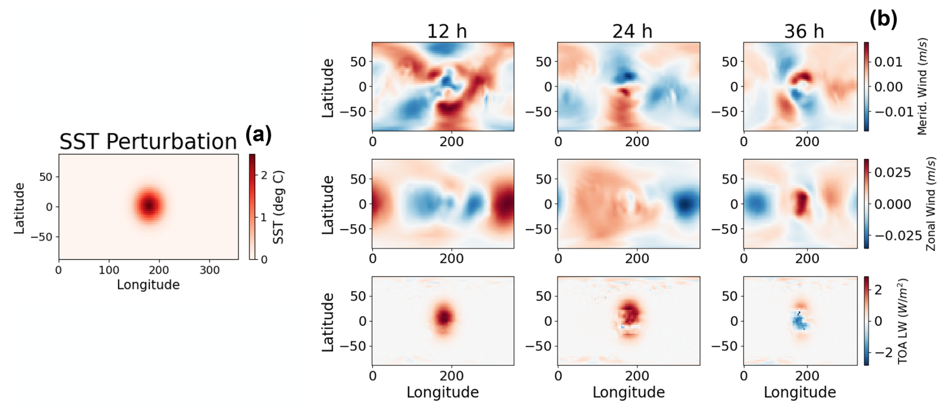
Figure 8 Influence of a sea surface temperature (SST) perturbation on the future model state. (a) Sea surface temperature (SST) perturbation in °C. (b) Changes to meridional wind (row 1), zonal wind (row 2), and outgoing longwave radiation at the top of the atmosphere (row 3) at 12 h (column 1), 24 h (column 2), and 36 h (column 3) in the future.

As an example, we show the influence of a sea surface temperature (SST) perturbation on the future state of a default JCM run. Here x is the SST forcing for the model run and f is the predicted meridional wind, zonal wind, and top-of-atmosphere outgoing longwave radiation. ℱ(x) is a function that executes the forward run of JCM with the given SSTs and isolates the desired predictions. We apply an SST perturbation, Δx, to obtain corresponding changes in the predictions, Δf. JVP propagates the perturbation (tangent vector) through the tangent linear model of ℱ(x). Figure 8a shows an example SST perturbation. Figure 8b shows the change in meridional wind, zonal wind, and TOA longwave radiation at 12, 24, and 36 h in the future. The localized warm SST anomaly centered near the equator drives a rapid, large-scale dynamical response in the upper-level winds, with both meridional and zonal wind perturbations propagating globally within 12–36 h. The alternating meridional wind response straddling the equator resembles Rossby wave dispersion from an equatorial heat source (Matsuno, 1966; Gill, 1980). The TOA outgoing longwave radiation response remains local to the SST forcing throughout the 36 h period, indicating that while the dynamical adjustment is fast and far-reaching, the thermodynamic/radiative response is still confined near the heating source on this timescale. JVP circumvents the need for large ensembles and finite differences to estimate model sensitivities and instead directly calculates those quantities.

As an alternative example, we analyze the sensitivity of the predicted top-of-atmosphere (TOA) outgoing longwave radiation with respect to the open-ocean surface albedo. Instead of perturbing a forcing field, we perturb a model parameter. In this scenario, our output f of the forward map ℱ(⋅) is the predicted TOA outgoing longwave radiation and our input x will be the JCM physics parameters. In order to extract the sensitivity of TOA outgoing longwave radiation to open-ocean surface albedo, we set all values of the tangent vector Δx to 0, except for the value corresponding to our parameter of interest which is set to 1. This method effectively extracts individual elements of the Jacobian. The gradient is always computed at the input value x₀, which in this case is the set of default parameter values from SPEEDY. The code block in Fig. 9 implements the described experiment, calculating the gradient of f (longwave_rad.ftop) with respect to the open-ocean surface albedo (Parameters.albsea) using JVP (jax.jvp). Figure 10 shows the output of this calculation, which is the sensitivity of TOA outgoing longwave radiation after one and two days of simulation to a unit perturbation in open-ocean albedo.

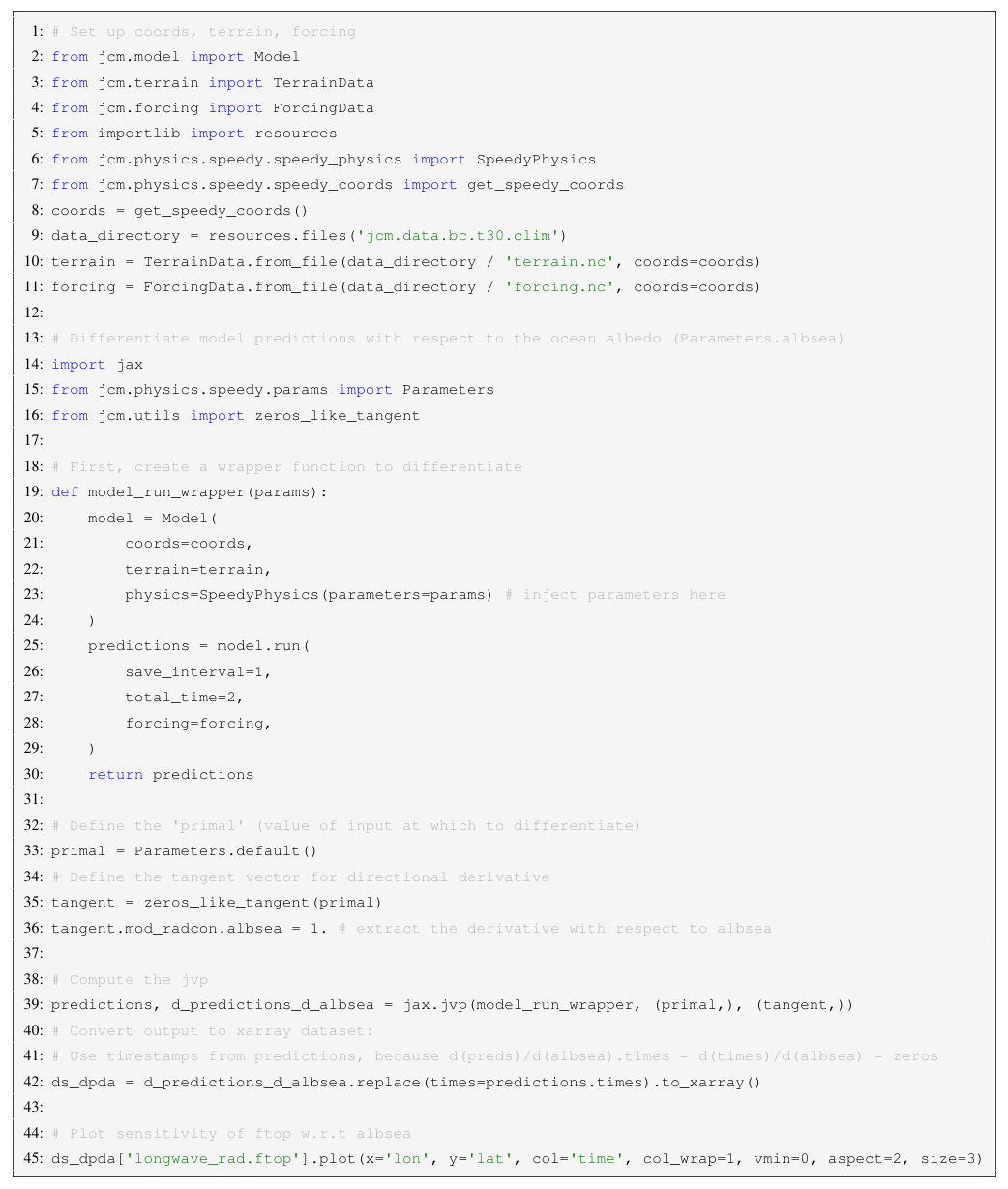
Figure 9 Using jax.jvp to compute the derivative of OLR with respect to the sea surface albedo parameter.

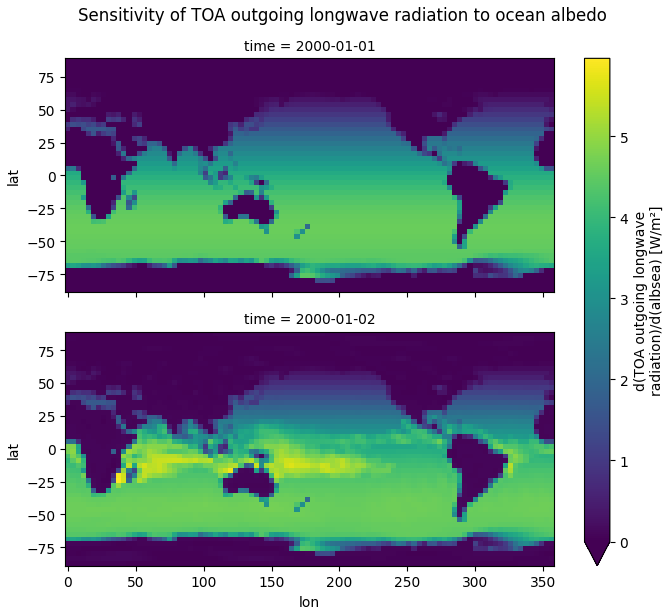
Figure 10 Derivative of predicted top-of-atmosphere outgoing longwave radiation with respect to changes in the sea-surface albedo parameter.

7 Conclusions

The JAX Circulation Model (JCM), is an open-source, differentiable atmospheric model written in Python using the JAX library. The design of JCM is user friendly and the software is hardware agnostic, making the model easy to run on personal machines while including capability for long, high-resolution simulations on GPUs and TPUs. Because it is written in Python, JCM is accessible to a wide range of developers, scientists, and educators. JCM v1.1 uses the SPEEDY model intermediate-complexity parameterizations which provide a valuable test bed for hybrid methodologies. Furthermore, model gradients obtained through automatic differentiation provide access to a broad set of optimization and estimation algorithms. These methods can be used for parameter estimation and sensitivity analysis, supporting experiments that serve to increase understanding of Earth system predictability. Tools such as JCM will help tackle unanswered climate science questions that are computationally challenging or require gradient information. Future JCM studies will test how gradient information changes the ability to calibrate atmospheric models against Earth observations. This will increase our understanding of climate model parameters and their effect on climate projections. We will continue investigating the JCM physics parameters through more realistic sensitivity experiments, providing insight on the dynamics and processes that drive atmospheric variability. These gradients can also be used to explore parameter uncertainty, where the efficiency of JAX will be advantageous to generate large ensembles.

JCM parameterizations are also flexible, meaning that physics schemes can be easily interchanged. “Plug-and-play” parameterizations allows for testing and intercomparison of new models and methods. ML architectures (i.e., neural networks) are currently under consideration to represent subgrid-scale processes that are poorly understood. In JCM, ML and traditional physics schemes can be tested side-by-side. ML components can be trained either offline or online within a calibration framework. Future versions of JCM will also include options with more comprehensive physics schemes such as parameterizations from the icosahedral nonhydrostatic (ICON) atmospheric general circulation model (Giorgetta et al., 2018). In parallel with JCM development, we are working towards a fully coupled ESM written in pure Python. This includes ongoing work to couple JCM to the Versatile Ocean Simulator (Veros; Häfner et al., 2021, 2018), along with efforts to integrate the Python and JAX land model, DifferLand (Fang et al., 2024). These next steps will extend the JCM framework, creating a lightweight, fully differentiable ESM framework that can aid in the acceleration of climate modeling research.