Version 3.0.2 of the Crocus snowpack model

This article presents a comprehensive description of the 3.0.2 stable release of the Crocus snowpack model in the SURFEX modelling platform. It synthesizes and harmonizes a number of equations disseminated in various previous publications, introduces a number of unpublished parameterizations and includes new developments implemented since 2012. Among the novelties, an explicit representation of the evolution of impurity mass in snow (e.g. black carbon, mineral dust) allows representing their impact on solar radiation absorption in the snowpack at different wavelengths and their feedback on all snowpack properties. The model also allows the formation of surface ice layers due to freezing rain. In addition, Crocus is coupled to the MEB “big-leaf” vegetation scheme and can therefore be applied in forested areas. A module for snow management can also be optionally activated to simulate the snowpack on ski slopes in ski resorts. The model can be coupled with various blowing snow schemes. The MEPRA expert system which analyses the mechanical stability of the simulated snowpack has been implemented directly within SURFEX. For each physical process represented by empirical parameterizations, several new parameterizations from the literature were implemented. The different combinations of these parameterizations constitute the ESCROC multiphysics ensemble model. It allows the quantification of simulations uncertainty for various applications. Finally, a technical solution was proposed for externalized applications allowing the use of the scheme in other Land Surface Models. The paper also reviews the available scientific evaluations and applications of the model. It describes its numerical efficiency and the main scientific and technical challenges providing guidance for the future of snow modelling.

1 Introduction

A large variety of snowpack modelling systems (e.g. Krinner et al., 2018) have been developed for several decades for various applications (Largeron et al., 2020): the computation of energy fluxes at the atmosphere-cryosphere interface in climate modelling and numerical weather prediction; hydrological simulations for discharge forecasting, water resources and hydropower management; physical process studies in the snowpack; avalanche hazard forecasting; glacier mass balance assessment; sea ice modelling; etc. The most detailed snowpack models include a detailed representation of the snowpack stratigraphy as well as an explicit representation of some microstructural properties of the snow layers through the implementation of empirical parameterization of snow metamorphism. There is a relatively limited number of snowpack models with such a level of detail: mainly the “Swiss” SNOWPACK model (Lehning et al., 1999), the “American” SNTHERM model (Jordan, 1991), the “Japanese” SMAP model (Niwano et al., 2012) and the “French” Crocus model. The latter has been initially developed by Brun et al. (1989, 1992) and was implemented in the early 2010s in the SURFEX platform of surface modelling (Masson et al., 2013) to facilitate coupling with atmospheric models and the other components of surface modelling, especially soil and vegetation schemes of the ISBA Land Surface Model. The last description of the model was published by Vionnet et al. (2012) after this major evolution.

However, numerous evolutions of the model have been implemented after Vionnet et al. (2012). Some of them are only partly described in dedicated scientific publications (Carmagnola et al., 2014; Spandre et al., 2016; Lafaysse et al., 2017; Tuzet et al., 2017; Vionnet et al., 2018; Quéno et al., 2018). These articles were generally published before the merging of all new developments in a unique and stable code version. A comprehensive and accurate description of the state of the last official model release is therefore missing. This lack of documentation has been identified by Menard et al. (2021) as one of the main factors of human errors in numerical simulations. The purpose of this paper is to provide an updated reference with all the functionalities available in the latest stable release of the model. To help the users to find any information they may need to understand the model implementation, all the equations disseminated in the various papers are reported here either in the main text or in Appendices, including the equations already published in previous references of Brun et al. (1992) and Vionnet et al. (2012) in order to provide a self-sufficient reference describing the whole model. Following the recommendations of Menard et al. (2021), a major effort has been dedicated to check the consistency and comprehensiveness between the code and the equations. The scope of this paper is limited to the snowpack on the ground. The coupled modules representing soil, vegetation and blowing snow remain beyond the scope of this paper and only the terms involved in the coupling are mentioned. More details can be found in the reference publications of the coupled models: Decharme et al. (2016); Boone et al. (2017) for soil and vegetation; Vionnet et al. (2014, 2018) and Baron et al. (2024) for blowing snow, cf. Sect. 2.4.2. Note that the standalone Crocus model was last designated as version 2.4. This versioning was discontinued by Vionnet et al. (2012) in favor of the SURFEX versioning system. However, due to the impossibility to synchronize Crocus and SURFEX main stable releases and the integration of Crocus in other Land Surface Models, a dedicated versioning is necessary for Crocus. This paper thus describes version 3.0.2 of Crocus. Section  refmodel presents all scientific equations necessary to evolve the state variables of the model. Section 3 presents complementary diagnoses computed as output of the model. Section 4 presents technical features associated with running the model (simulation geometries, numerical efficiency, and associated tools to facilitate running and visualization). Finally, Sect. 5 reviews the available scientific evaluations of the model and provides an overview of its applications. In light of these elements, we discuss the confidence that can be placed in the simulation results and the main remaining challenges for the future, including perspectives in terms of data assimilation.

2 Physical model

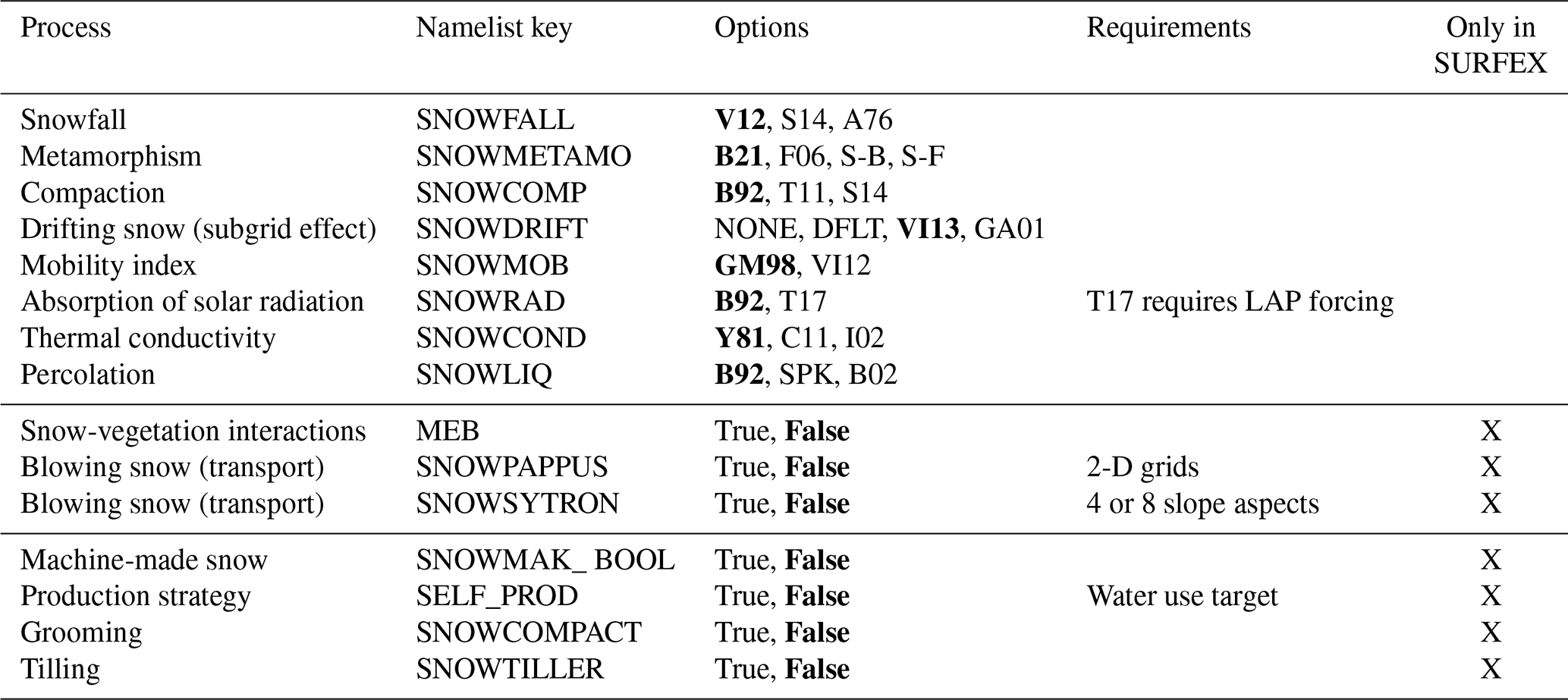
Compared to Vionnet et al. (2012), the model has become highly modular with the extension of applications and the development of the ESCROC multiphysics framework by Lafaysse et al. (2017). The common modelling structure includes the discretization procedure and the solving of the heat diffusion equation which is the core of the model. Figure 1 presents an overview of the sequence of routines and summarizes the main changes (new routines and updated routines) which are detailed in this section. Table 1 summarizes the different available options for each process and associated requirements. The details of each option are described in the subsection dedicated to the corresponding process. The ESCROC multiphysics ensemble system consists in the combination of these differents physical options and different values of some key parameters such as τ_a (Sect. 2.4.9), Ri_l (Sect. 2.4.11).

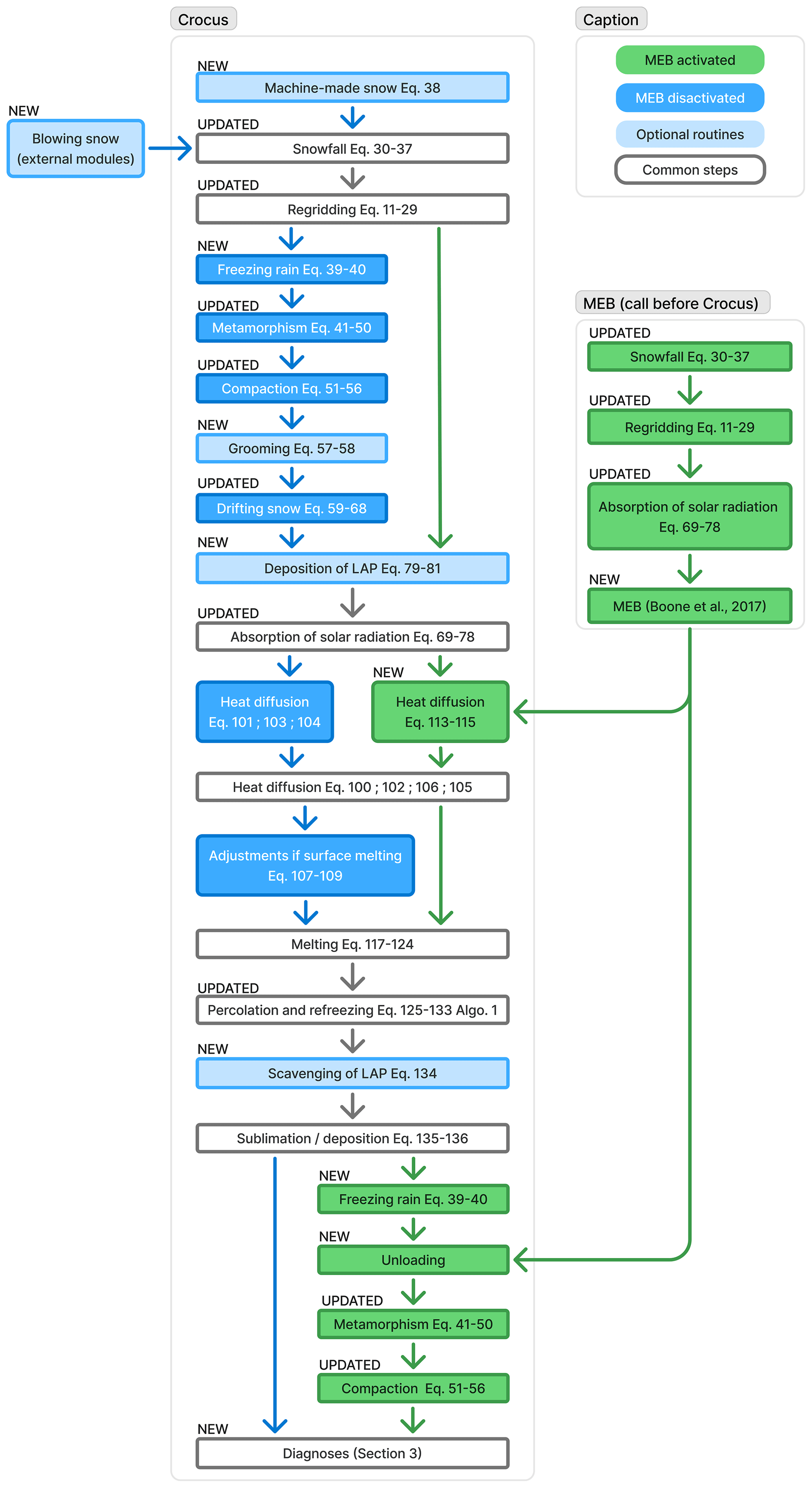
Figure 1 Sequence of Crocus subroutines for each time step without (blue) or with (green) coupling with MEB. Optional subroutines in light blue. Compared to the version of Vionnet et al. (2012), new subroutines are labelled “NEW”. The label “UPDATED” refers to subroutines in which changes were applied due to the new state variables for microstructure and where new physical options were implemented. The heat diffusion, melting and sublimation routines were only concerned by minor changes or technical optimizations.

Table 1 Available physical options in Crocus. Default options appear in bold. The last column shows options which are not available in the externalized release but only within the SURFEX implementation of Crocus. Although the combination of all options is possible in theory, the options for snow management in ski resorts were only tested with the default options of the other processes and the blowing snow schemes were never tested together with the MEB vegetation scheme.

2.1 Forcing variables

The model has to be forced with subdaily time series of air temperature T_a (K) and specific humidity q_a (kg kg⁻¹) at a known level z_a (m), wind speed U (m s⁻¹) at a known level z_u (m), incoming longwave radiation LW↓ (W m⁻²), incoming shortwave direct and diffuse radiation SW_DIR↓ and SW_DIF↓ (W m⁻²), rainfall 𝒫_r and snowfall 𝒫_s (kg m⁻² s⁻¹) and surface pressure P_s (Pa). The very low sensitivity of model results to P_s allows the user to provide constant P_s values when a time series is not available. The split of global shortwave radiation SW↓ between direct and diffuse components is only used with specific model options (coupling with TARTES optical scheme, Sect. 2.4.9, and/or coupling with MEB big-leaf vegetation scheme, Sect. 2.4.14). When none of these options are activated, the split between both components is not necessary as only their sum is considered. When TARTES or MEB are activated, an accurate forcing of SW_DIR↓ and SW_DIF↓ should always be preferred. Nevertheless, for users interested in these options without available data to separate both components, the following parameterization as a function of the cosine of the solar zenithal angle μ and derived from SBDART clear-sky modelling (Ricchiazzi et al., 1998) at Col de Porte is available for mid-latitude areas. Following Gardner and Sharp (2010), the estimated error in cloudy conditions for the simulated broadband albedo is lower than 0.1. The parameterization is applied by default in the code if the diffuse component is set to zero:

$$\begin{array}{}\text{(1)}& {\displaystyle \frac{{\mathrm{SW}}_{\mathrm{DIF}}}{{\mathrm{SW}}_{\mathrm{DIR}}+{\mathrm{SW}}_{\mathrm{DIF}}}}=\min \left(\exp \left(-\mathrm{1.549919}{\mathit{\mu }}^{\mathrm{3}}+\mathrm{3.735357}{\mathit{\mu }}^{\mathrm{2}}-\mathrm{3.524211}\mathit{\mu }+\mathrm{0.029911}\right),\mathrm{1}.\right).\end{array}$$

Optionally, dry and wet deposition fluxes of Light-Absorbing Particles (LAP) 𝒲_d,j and 𝒲_w,j (kg m⁻² s⁻¹) can be included for each type j depending on the physical option selected for radiative transfer (Sect. 2.4.9).

2.2 State variables

The prognostic variables (i.e. transmitted from a given time step to the next one) describing each snow layer i are its mass m_i (kg m⁻²), density ρ_i (kg m⁻³), enthalpy H_i (J m⁻²) defined as the energy required to melt the snow layer i (Boone and Etchevers, 2001), age A_i (days since snowfall), and complementary variables for snow microstructure. The state variables initially used for snow microstructure as described in Vionnet et al. (2012) (dendricity, sphericity, grain size) were replaced by optical diameter d_i (m) and sphericity $S_i\in [\mathrm{0},\mathrm{1}]$ (Carmagnola et al., 2014). After several years of coexistence, the formulation from Brun et al. (1992) was removed from the code in order to improve its readability but also its efficiency as numerous expensive conditional statements could be removed. This change of state variables does not only affect metamorphism evolution laws but also various equations based on microstructure properties in other simulated processes. All modified equations are provided in the following section or in an appendix. In addition, a historical tracker h_i is used as a last state variable with its meaning summarized in Table 2.

Table 2 Possible values of the historical tracker h_i.

Light Absorbing Particles (LAP) are organic or mineral substances able to increase radiation absorption in snow. Tuzet et al. (2017) added LAP mass contents ℳ_i,j (kg m⁻²) as new optional state variables for each layer i and LAP type j. Although the code is designed to deal with any number of LAP types, only the parameters corresponding to black carbon and mineral dust are implemented in version 3.0.2. LAP interact with the other variable states of the model through absorption of solar radiation when the TARTES optical scheme is activated (Sect. 2.4.9).

Note that the layer thickness z_i (m), the layer temperature T_i (K) and the layer mass of liquid water l_i (kg m⁻²) can be directly derived from the state variables and are used in many parts of the model.

$$\begin{array}{}\text{(2)}& {\displaystyle }& {\displaystyle }{z}_i={\displaystyle \frac{m_i}{{\mathit{\rho }}_i}}\text{(3)}& {\displaystyle }& {\displaystyle }{T}_i=\min \left(T_{\mathrm{0}},T_i^{*}\right)\text{(4)}& {\displaystyle }& {\displaystyle }{l}_i=\max \left(\mathrm{0},T_i^{*}-T_{\mathrm{0}}\right){\displaystyle \frac{m_i{c}_{\mathrm{I}}}{L_m}}\end{array}$$

where

$$\begin{array}{}\text{(5)}& T_i^{*}=T_{\mathrm{0}}+{\displaystyle \frac{H_i}{m_i{c}_{\mathrm{I}}}}+{\displaystyle \frac{L_m}{c_{\mathrm{I}}}}.\end{array}$$

T₀ (K) is the water melting point temperature which in SURFEX is assumed to be equal to the triple point value. L_m (J kg⁻¹) is the latent heat of fusion, and c_I (J kg⁻¹ K⁻¹) the ice thermal capacity. Note also that the temperature θ_i in °C is also used in some parameterizations:

$$\begin{array}{}\text{(6)}& {\mathit{\theta }}_i=T_i-T_{\mathrm{0}}.\end{array}$$

2.3 Layering

2.3.1 Vertical discretization

One of the main original feature of Crocus compared to the majority of snowpack schemes available in the literature is its Lagrangian vertical discretization based on a dynamical evolution of the number and thicknesses of the numerical snow layers. The number of active layers N varies between N_min=3 and a user-defined maximum N_max (the default value is 50). Each layer is referenced by the index i which varies from 1 for the surface layer to N for the deepest layer. The main discretization principles described in Vionnet et al. (2012) are still valid in the current version but they have been a bit complexified to solve numerical issues in specific applications. The current article provides the first comprehensive formulation of the algorithm.

First, a similarity criterion $D(i,i+\mathrm{1})$ between adjacent layers i and i+1 is defined. The initial formulation was a Manhattan distance of weighted values of dendricity, sphericity and grain size but it has never been published. The strict variable transformation of Carmagnola et al. (2014) led to a unjustified complexity in the formulation of this distance. Therefore, this distance was simplified in the same spirit by:

$$\begin{array}{}\text{(7)}& \left\{\begin{array}{cll}D(i,i+\mathrm{1})& =\mathrm{50}\left(|S_{i+\mathrm{1}}-S_i|+\mathrm{2000}|d_{i+\mathrm{1}}-d_i|+{\mathit{\delta }}_h(i,i+\mathrm{1})\right)& \mathrm{if}\left(A_i-A_{i+\mathrm{1}}\right)<\mathrm{300}\\ D(i,i+\mathrm{1})& =\mathrm{200}& \mathrm{otherwise}\end{array}\right.\end{array}$$

where

$$\begin{array}{}\text{(8)}& \left\{\begin{array}{cl}{\mathit{\delta }}_h(i,i+\mathrm{1})=\mathrm{1}& \mathrm{if}\left(h_i>\mathrm{1}\mathrm{and}{h}_{i+\mathrm{1}}\le \mathrm{1}\right)\mathrm{or}\left(h_i\le \mathrm{1}\mathrm{and}{h}_{i+\mathrm{1}}>\mathrm{1}\right)\\ {\mathit{\delta }}_h(i,i+\mathrm{1})=\mathrm{0}& \mathrm{otherwise}\end{array}\right..\end{array}$$

The 2000 coefficient is chosen for normalization considering the typical range of $\mathrm{5}\times {\mathrm{10}}^{-\mathrm{4}}$ m between highest and lowest values of d_i (Carmagnola et al., 2014) and the range of 1 between highest and lowest values of S_i. The δ_h function avoids the aggregation between cold snow and wet/refrozen snow. The specific case of significant age difference was introduced to avoid the aggregation of a recent snow layer with layers describing permanent snow or glacier. This distance is noted D(n,1) when it is applied between a new snowfall and the surface layer.

When it is necessary to choose two layers to aggregate, a penalty criteria $P(i,i+\mathrm{1})$ is defined by:

$$\begin{array}{}\text{(9)}& P(i,i+\mathrm{1})=D(i,i+\mathrm{1})+\mathrm{25}\left({\displaystyle \frac{z_i}{z_i^{*}}}+{\displaystyle \frac{z_{i+\mathrm{1}}}{z_{i+\mathrm{1}}^{*}}}\right)\end{array}$$

where $z_i^{*}$ (m) is the layer thickness of the optimal attractor profile defined in Appendix A.

Layers l_sup and l_inf are the adjacent layers which satisfy:

$$\begin{array}{}\text{(10)}& P\left(l_{\sup },l_{\inf }\right)={\min }_{i\in [\mathrm{1},N-\mathrm{1}]}\left(P\right(i,i+\mathrm{1}\left)\right).\end{array}$$

The algorithm modifies the thicknesses at the previous time step $z_i^{t-\mathrm{\Delta }t}$ for $i\in [\mathrm{1},N^{t-\mathrm{\Delta }t}]$ towards a new profile $z_i^t$ for $i\in [\mathrm{1},N^t]$ following Eq. (11) by a succession of exclusive conditional statements depending on the total initial depth $Z^{t-\mathrm{\Delta }t}=\sum i={\mathrm{1}}^N{z}_i^{t-\mathrm{\Delta }t}$, the initial thickness of the first layer $z_{\mathrm{1}}^{t-\mathrm{\Delta }t}$, the thickness of new snowfall to add $z_{\mathrm{n}}=\frac{m_{\mathrm{n}}}{{\mathit{\rho }}_n}$ (m), and the initial number of layers N^t−Δt. The computations of the mass m_n (kg m⁻²) and density of new snowfall ρ_n (kg m⁻³) are described later in Sect. 2.4.1.

$$\begin{array}{}\text{(11)}& \left\{\begin{array}{l}\mathrm{If}{z}_{\mathrm{n}}>\mathrm{0}\left\{\begin{array}{l}\left[\begin{array}{r}{\displaystyle }\mathrm{If}{Z}^{t-\mathrm{\Delta }t}<Z_{\min }\\ {\displaystyle }\mathrm{or}{N}^{t-\mathrm{\Delta }t}<N_{\min }\end{array}\right]\left\{\begin{array}{l}{N}^t=\max \left[N_{\min },\min \left(N_{\max },\lfloor \mathrm{100}{z}_n\rfloor \right)\right]\\ z_i^t=\frac{z_{\mathrm{n}}}{N^t}\forall i\in \left[\mathrm{1},N^t\right]\end{array}\right.\\ \mathrm{else}\left\{\begin{array}{l}\left[\begin{array}{r}{\displaystyle }\mathrm{If}{z}_{\mathrm{1}}^{t-\mathrm{\Delta }t}<z_{\mathrm{1}}^{*}\mathrm{and}D(n,\mathrm{1})<\mathrm{0.2}\\ {\displaystyle }\mathrm{or}{\displaystyle \frac{m_{\mathrm{n}}}{\mathrm{\Delta }t}}<\mathrm{3}\times {\mathrm{10}}^{-\mathrm{5}}\mathrm{kg}{\mathrm{m}}^{-\mathrm{2}}{\mathrm{s}}^{-\mathrm{1}}\mathrm{and}{z}_{\mathrm{1}}<\mathrm{2}{z}_{\mathrm{1}}^{*}\\ {\displaystyle }\mathrm{or}{z}_{\mathrm{1}}^{t-\mathrm{\Delta }t}<{\mathrm{10}}^{-\mathrm{4}}\end{array}\right]\left\{\begin{array}{l}{N}^t=N^{t-\mathrm{\Delta }t}\\ z_{\mathrm{1}}^t=z_{\mathrm{1}}^{t-\mathrm{\Delta }t}+z_{\mathrm{n}}\\ z_i^t=z_i^{t-\mathrm{\Delta }t}\forall i\in \left[\mathrm{2},N^t\right]\end{array}\right.\\ \mathrm{else}\left\{\begin{array}{l}\mathrm{If}{N}^{t-\mathrm{\Delta }t}<N_{\max }\left\{\begin{array}{l}{N}^t=N^{t-\mathrm{\Delta }t}+\mathrm{1}\\ z_{\mathrm{1}}^t=z_{\mathrm{n}}\\ z_i^t=z_{i-\mathrm{1}}^{t-\mathrm{\Delta }t}\forall i\in \left[\mathrm{2},N^t\right]\end{array}\right.\\ \mathrm{else}\left\{\begin{array}{l}{N}^t=N_{\max }\\ z_{\mathrm{1}}^t=z_{\mathrm{n}}\\ z_i^t=z_{i-\mathrm{1}}^{t-\mathrm{\Delta }t}\forall i\in \left[\mathrm{2},l_{\sup }\right]\\ z_{l_{\inf }}^t=z_{l_{\sup }}+z_{l_{\inf }}\\ z_i^t=z_i^{t-\mathrm{\Delta }t}\forall i\in \left[l_{\inf }+\mathrm{1},N_{\max }\right]\end{array}\right.\end{array}\right.\end{array}\right.\end{array}\right.\\ \mathrm{else}\left\{\begin{array}{l}\mathrm{If}{z}_{\mathrm{1}}^{t-\mathrm{\Delta }t}<\mathrm{5}\times {\mathrm{10}}^{-\mathrm{3}}\left\{\begin{array}{l}{N}^t=N^{t-\mathrm{\Delta }t}-\mathrm{1}\\ z_{\mathrm{1}}^t=z_{\mathrm{1}}^{t-\mathrm{\Delta }t}+z_{\mathrm{2}}^{t-\mathrm{\Delta }t}\\ z_i^t=z_{i+\mathrm{1}}^{t-\mathrm{\Delta }t}\forall i\in \left[\mathrm{2},N^t\right]\end{array}\right.\\ \mathrm{else}\left\{\begin{array}{l}\mathrm{If}{z}_{N^{t-\mathrm{\Delta }t}}^{t-\mathrm{\Delta }t}<{\mathrm{10}}^{-\mathrm{2}}\left\{\begin{array}{l}{N}^t=N^{t-\mathrm{\Delta }t}-\mathrm{1}\\ z_i^t=z_i^{t-\mathrm{\Delta }t}\forall i\in \left[\mathrm{1},N^t-\mathrm{1}\right]\\ z_{N^t}^t=z_{N^t}^{t-\mathrm{\Delta }t}+z_{N^t+\mathrm{1}}^{t-\mathrm{\Delta }t}\end{array}\right.\\ \mathrm{else}\left\{\begin{array}{l}\mathrm{If}\exists j\in \left[\mathrm{1},\min \left(N^t-\mathrm{1},N_{\max }-\mathrm{4}\right)\right]|z_j^{t-\mathrm{\Delta }t}>\left(\mathrm{8}-\frac{N_{\max }-N^{t-\mathrm{\Delta }t}}{N^{t-\mathrm{\Delta }t}-N_{\min }}\right)z_j^{*}\left\{\begin{array}{l}{N}^t=N^{t-\mathrm{\Delta }t}+\mathrm{1}\\ z_i^t=z_i^{t-\mathrm{\Delta }t}\forall i\in [\mathrm{1},j-\mathrm{1}]\\ z_i^t=\frac{z_j^{t-\mathrm{\Delta }t}}{\mathrm{2}}\forall i\in [j,j+\mathrm{1}]\\ z_i^t=z_{i-\mathrm{1}}^{t-\mathrm{\Delta }t}\forall i\in \left[j+\mathrm{2},N^t\right]\end{array}\right.\\ \mathrm{else}\left\{\begin{array}{l}\mathrm{If}\exists j\in \left[\mathrm{2},N^t-\mathrm{1}\right]|\left[\begin{array}{r}{\displaystyle }{z}_j^{t-\mathrm{\Delta }t}<{\displaystyle \frac{\mathrm{5}{z}_j^{*}}{D(i,i+\mathrm{1})}}\\ {\displaystyle }\mathrm{and}\left(z_j^{t-\mathrm{\Delta }t}+z_{j+\mathrm{1}}^{t-\mathrm{\Delta }t}\right)<\mathrm{4.5}\max \left(z_j^{*},z_{j+\mathrm{1}}^{*}\right)\end{array}\right]\left\{\begin{array}{l}{N}^t=N^{t-\mathrm{\Delta }t}-\mathrm{1}\\ z_i^t=z_i^{t-\mathrm{\Delta }t}\forall i\in [\mathrm{1},j-\mathrm{1}]\\ z_j^t=z_j^{t-\mathrm{\Delta }t}+z_{j+\mathrm{1}}^{t-\mathrm{\Delta }t}\\ z_i^t=z_{i+\mathrm{1}}^{t-\mathrm{\Delta }t}\forall i\in \left[j+\mathrm{1},N^t\right]\end{array}\right.\\ \mathrm{else}\left\{\begin{array}{l}{N}^t=N^{t-\mathrm{\Delta }t}\\ z_i^t=z_i^{t-\mathrm{\Delta }t}\forall i\in \left[\mathrm{1},N^t\right]\end{array}\right.\end{array}\right.\end{array}\right.\end{array}\right.\end{array}\right.\end{array}\right..\end{array}$$

In the definition of the initial number of layers (first line of Eq. (11)), ⌊.⌋ designates the floor operator. The literal translation of Eq. (11) is as follows. A uniform layering is applied for new snowfall on the ground while the total snow depth does not reach Z_min=0.03 m. In other cases, snowfall is aggregated to the surface layer when it is similar to a sufficiently thin surface layer or when it is very low. When new snowfall is too thick or too different from the surface layer, a new layer is created. However, if N_max was already reached, this layer creation is done after the preliminary aggregation of the two closest layers of the profile l_sup and l_inf (as defined by Eq. 10). When there is no snowfall, the algorithm applies only one of the following modification by order of priority: aggregation of surface layer or bottom layer when too thin, split of internal layer when too thick, aggregation of internal layer when too thin, relative to the optimal attractor profile. Note than only one modification by point is allowed at each time step. Thus, when the conditions for an internal split or aggregation are obtained for several layers (i.e. several values of j) at the same time, it is only applied for the uppermost layer min(j). For glacier applications, aggregation is strictly forbidden between snow and ice layers (i.e. when ρ_i<ρ_G and ${\mathit{\rho }}_{i+\mathrm{1}}>{\mathit{\rho }}_{\mathrm{G}}$ where the threshold density for glacier ρ_G can be adjusted by the user (default 850 kg m⁻³).

This algorithm is applied independently at each simulation point. Therefore, the vertical layering differs between points in terms of number and thickness of snow layers. This raises a number of vectorization issues in the management of loops which were the topic of recent investigations detailed in Appendix J.

2.3.2 Aggregation of layers

When two layers i and i+1 are aggregated ($z_i^t=z_i^{t-\mathrm{\Delta }t}+z_{i+\mathrm{1}}^{t-\mathrm{\Delta }t}$ from Eq. 11) the state variables are modified in order to conserve mass and enthalpy. The optical diameter is updated in order to obtain a mass-weighted average of the corresponding albedo. A mass-weighted average is also applied for sphericity and age.

$$\begin{array}{}\text{(12)}& {\displaystyle }{m}_i^t=m_i^{t-\mathrm{\Delta }t}+m_{i+\mathrm{1}}^{t-\mathrm{\Delta }t}\text{(13)}& {\displaystyle }{\mathit{\rho }}_i^t={\displaystyle \frac{m_i^t}{z_i^t}}\text{(14)}& {\displaystyle }{H}_i^t=H_i^{t-\mathrm{\Delta }t}+H_{i+\mathrm{1}}^{t-\mathrm{\Delta }t}\text{(15)}& {\displaystyle }{d}_i^t={\left[{\displaystyle \frac{\mathrm{0.9}-\frac{m_i^{t-\mathrm{\Delta }t}\left(\mathrm{0.9}-\mathrm{15.4}\sqrt{d_i^{t-\mathrm{\Delta }t}}\right)+m_{i+\mathrm{1}}^{t-\mathrm{\Delta }t}\left(\mathrm{0.9}-\mathrm{15.4}\sqrt{d_{i+\mathrm{1}}^{t-\mathrm{\Delta }t}}\right)}{m_i+m_{i+\mathrm{1}}}}{\mathrm{15.4}}}\right]}^{\mathrm{2}}\text{(16)}& {\displaystyle }{S}_i^t={\displaystyle \frac{m_i^{t-\mathrm{\Delta }t}{S}_i^{t-\mathrm{\Delta }t}+m_{i+\mathrm{1}}^{t-\mathrm{\Delta }t}{S}_{i+\mathrm{1}}^{t-\mathrm{\Delta }t}}{m_i+m_{i+\mathrm{1}}}}\text{(17)}& {\displaystyle }{A}_i^t={\displaystyle \frac{m_i^{t-\mathrm{\Delta }t}{A}_i^{t-\mathrm{\Delta }t}+m_{i+\mathrm{1}}^{t-\mathrm{\Delta }t}{A}_{i+\mathrm{1}}^{t-\mathrm{\Delta }t}}{m_i+m_{i+\mathrm{1}}}}\text{(18)}& {\displaystyle }{h}_i^t=\left\{\begin{array}{ll}{h}_i^{t-\mathrm{\Delta }t}& \mathrm{if}{m}_i^{t-\mathrm{\Delta }t}\ge m_{i+\mathrm{1}}^{t-\mathrm{\Delta }t}\\ h_{i+\mathrm{1}}^{t-\mathrm{\Delta }t}& \mathrm{otherwise}\end{array}\right.\text{(19)}& {\displaystyle }{\mathcal{W}}_{\mathrm{d},i}^t={\mathcal{W}}_{\mathrm{d},i}^{t-\mathrm{\Delta }t}+{\mathcal{W}}_{\mathrm{d},i+\mathrm{1}}^{t-\mathrm{\Delta }t}\text{(20)}& {\displaystyle }{\mathcal{W}}_{\mathrm{w},i}^t={\mathcal{W}}_{\mathrm{w},i}^{t-\mathrm{\Delta }t}+{\mathcal{W}}_{\mathrm{w},i+\mathrm{1}}^{t-\mathrm{\Delta }t}\end{array}$$

The same equations apply to aggregate falling snow with the surface layer replacing $x_i^t$, $x_i^{t-\mathrm{\Delta }t}$ and $x_{i+\mathrm{1}}^{t-\mathrm{\Delta }t}$ by respectively $x_{\mathrm{1}}^t$, $x_{\mathrm{1}}^{t-\mathrm{\Delta }t}$ and x_n for each x representing all state variables m, ρ, H, d, S, A, h, 𝒲_d and 𝒲_w in Eqs. (12)–(20).

2.3.3 Splitting of layers

When a layer i is split into two layers i and i+1 ($z_i^t=z_{i+\mathrm{1}}^t=\frac{z_i^{t-\mathrm{\Delta }t}}{\mathrm{2}}$ from Eq. 11), mass and enthalpy are divided into equal parts and microstructure properties are not modified:

$$\begin{array}{}\text{(21)}& {\displaystyle }& {\displaystyle }{m}_i^t=m_{i+\mathrm{1}}^t={\displaystyle \frac{m_i^{t-\mathrm{\Delta }t}}{\mathrm{2}}}\text{(22)}& {\displaystyle }& {\displaystyle }{\mathit{\rho }}_i^t={\displaystyle \frac{m_i^t}{z_i^t}}\text{(23)}& {\displaystyle }& {\displaystyle }{H}_i^t=H_{i+\mathrm{1}}^t={\displaystyle \frac{H_i^{t-\mathrm{\Delta }t}}{\mathrm{2}}}\text{(24)}& {\displaystyle }& {\displaystyle }{d}_i^t=d_{i+\mathrm{1}}^t=d_i^{t-\mathrm{\Delta }t}\end{array}$$

$$\begin{array}{}\text{(25)}& {\displaystyle }& {\displaystyle }{S}_i^t=S_{i+\mathrm{1}}^t=S_i^{t-\mathrm{\Delta }t}\text{(26)}& {\displaystyle }& {\displaystyle }{A}_i^t=A_{i+\mathrm{1}}^t=A_i^{t-\mathrm{\Delta }t}\text{(27)}& {\displaystyle }& {\displaystyle }{h}_i^t=h_{i+\mathrm{1}}^t=h_i^{t-\mathrm{\Delta }t}\text{(28)}& {\displaystyle }& {\displaystyle }{\mathcal{W}}_{\mathrm{d},i}^t={\mathcal{W}}_{\mathrm{d},i+\mathrm{1}}^t={\displaystyle \frac{{\mathcal{W}}_{\mathrm{w},i}^{t-\mathrm{\Delta }t}}{\mathrm{2}}}\text{(29)}& {\displaystyle }& {\displaystyle }{\mathcal{W}}_{\mathrm{w},i}^t={\mathcal{W}}_{\mathrm{w},i+\mathrm{1}}^t={\displaystyle \frac{{\mathcal{W}}_{\mathrm{w},i}^{t-\mathrm{\Delta }t}}{\mathrm{2}}}.\end{array}$$

2.4 Evolution equations

2.4.1 Snowfall

The new snow amount is the result of solid precipitation, but also deposition of blowing snow and snowmaking, when the corresponding modules are activated. These three mass sources are respectively referred by the subscripts SP, BS and SM in the following. In case of simultaneous occurrence, only one additional layer is created with weighted physical properties. Thus, the mass of the new layer is defined by:

$$\begin{array}{}\text{(30)}& m_{\mathrm{n}}=m_{\mathrm{SP}}+m_{\mathrm{BS}}+m_{\mathrm{SM}}.\end{array}$$

The density of new snow ρ_n, optical diameter d_n, and sphericity S_n are expressed by:

$$\begin{array}{}\text{(31)}& {\displaystyle }& {\displaystyle }{\mathit{\rho }}_{\mathrm{n}}={\displaystyle \frac{{\mathit{\rho }}_{\mathrm{SP}}{m}_{\mathrm{SP}}+{\mathit{\rho }}_{\mathrm{BS}}{m}_{\mathrm{BS}}+{\mathit{\rho }}_{\mathrm{SM}}{m}_{\mathrm{SM}}}{m_{\mathrm{n}}}}\text{(32)}& {\displaystyle }& {\displaystyle }{d}_{\mathrm{n}}={\displaystyle \frac{d_{\mathrm{SP}}{m}_{\mathrm{SP}}+d_{\mathrm{BS}}{m}_{\mathrm{BS}}+d_{\mathrm{SM}}{m}_{\mathrm{SM}}}{m_{\mathrm{n}}}}\text{(33)}& {\displaystyle }& {\displaystyle }{S}_{\mathrm{n}}={\displaystyle \frac{S_{\mathrm{SP}}{m}_{\mathrm{SP}}+S_{\mathrm{BS}}{m}_{\mathrm{BS}}+S_{\mathrm{SM}}{m}_{\mathrm{SM}}}{m_{\mathrm{n}}}}\end{array}$$

The mass of solid precipitation during the time step Δt is directly provided by the forcing:

$$\begin{array}{}\text{(34)}& m_{\mathrm{SP}}={\mathcal{P}}_{\mathrm{s}}\mathrm{\Delta }t.\end{array}$$

Several empirical expressions of the density of natural falling snow ρ_SP are implemented (Vionnet et al., 2012; Schmucki et al., 2014; Anderson, 1976), as a function of 2 m air temperature $T_{\mathrm{a}}^{*}$ (°C) $=T_{\mathrm{a}}-T_{\mathrm{0}}$ and 10 m wind speed U₁₀ (m s⁻¹). They can be activated through the SNOWFALL physical option following Eq. (35). An illustration comparing these formulations is provided in Lafaysse et al. (2017), Fig. 1 in the corrigendum. The parameters are listed in Appendix K3. When the forcing wind speed is not available at a 10 m height, a logarithmic adjustment is applied following Appendix B.

$$\begin{array}{}\text{(35)}& \left\{\begin{array}{l}\mathrm{If}\mathrm{SNOWFALL}=\mathrm{V}\mathrm{12}:{\mathit{\rho }}_{\mathrm{SP}}=\max \left({\mathit{\rho }}_{\min },a_{\mathit{\rho }}+b_{\mathit{\rho }}{T}_{\mathrm{a}}^{*}+c_{\mathit{\rho }}\sqrt{U_{\mathrm{10}}}\right)\\ \mathrm{If}\mathrm{SNOWFALL}=\mathrm{S}\mathrm{14}:\left\{\begin{array}{ll}{\log }_{\mathrm{10}}\left({\mathit{\rho }}_{\mathrm{SP}}\right)=e_{\mathit{\rho }}+f_{\mathit{\rho }}{T}_{\mathrm{a}}^{*}+g_{\mathit{\rho }}+h_{\mathit{\rho }}{\sin }^{-\mathrm{1}}\left(\sqrt{i_{\mathit{\rho }}}\right)+j_{\mathit{\rho }}{\log }_{\mathrm{10}}\left(\max \left[U_{\mathrm{10}},\mathrm{2}\right]\right)& \mathrm{if}{T}_{\mathrm{a}}^{*}\ge -\mathrm{14}\mathit{°}\mathrm{C}\\ {\log }_{\mathrm{10}}\left({\mathit{\rho }}_{\mathrm{SP}}\right)=e_{\mathit{\rho }}+f_{\mathit{\rho }}{T}_{\mathrm{a}}^{*}+h_{\mathit{\rho }}{\sin }^{-\mathrm{1}}\left(\sqrt{i_{\mathit{\rho }}}\right)+j_{\mathit{\rho }}{\log }_{\mathrm{10}}\left(\max \left[U_{\mathrm{10}},\mathrm{2}\right]\right)& \mathrm{otherwise}\end{array}\right.\\ \mathrm{If}\mathrm{SNOWFALL}=\mathrm{A}\mathrm{76}:{\mathit{\rho }}_{\mathrm{SP}}={\mathit{\rho }}_{\min }+\max \left(k_{\mathit{\rho }}{\left(T_{\mathrm{a}}^{*}+l_{\mathit{\rho }}\right)}^{\mathrm{1.5}},\mathrm{0}\right).\end{array}\right.\end{array}$$

Adjustments of parameter c_ρ were proposed by Woolley et al. (2024) to account for the uncertainties associated with the impact of wind speed on Arctic snowfall density. Although hard-coded in version 3.0.2, this parameter will be tunable in a future version.

Several formulations of microstructure properties of new snow were implemented by Vionnet et al. (2018) depending on SNOWDRIFT option. Again, Appendix B is used to assess the 5 m wind speed U₅ from the forcing wind speed U at height z_u. SNOWDRIFT options are reformulated here with the new microstructure variables now used in the model:

$$\begin{array}{}\text{(36)}& \left\{\begin{array}{l}\mathrm{If}\mathrm{SNOWDRIFT}=\mathrm{NONE}\left\{\begin{array}{l}{S}_{\mathrm{SP}}=\min \left(\max \left(\mathrm{0.0795}{U}_{\mathrm{5}}+\mathrm{0.38},\mathrm{0.5}\right),\mathrm{0.9}\right)\\ d_{\mathrm{SP}}={\mathrm{10}}^{-\mathrm{4}}\left({\mathit{\delta }}_{\mathrm{NONE}}+\left(\mathrm{1}-{\mathit{\delta }}_{\mathrm{NONE}}\right)\left(\mathrm{4}-S_{\mathrm{SP}}\right)\right)\\ \mathrm{where}{\mathit{\delta }}_{\mathrm{NONE}}=\min \left(\max \left(\mathrm{1.29}-\mathrm{0.173}{U}_{\mathrm{5}},\mathrm{0.2}\right),\mathrm{1}\right)\end{array}\right.\\ \mathrm{If}\mathrm{SNOWDRIFT}=\mathrm{DFLT}\left\{\begin{array}{l}{S}_{\mathrm{SP}}=\mathrm{0.5}\\ d_{\mathrm{SP}}={\mathrm{10}}^{-\mathrm{4}}\end{array}\right.\\ \mathrm{If}\mathrm{SNOWDRIFT}=\mathrm{VI}\mathrm{13}\left\{\begin{array}{l}{S}_{\mathrm{SP}}=\min \left(\max \left(\mathrm{0.035}{U}_{\mathrm{5}}+\mathrm{0.43},\mathrm{0.5}\right),\mathrm{0.9}\right)\\ d_{\mathrm{SP}}={\mathrm{10}}^{-\mathrm{4}}\left({\mathit{\delta }}_{\mathrm{VI}\mathrm{13}}+\left(\mathrm{1}-{\mathit{\delta }}_{\mathrm{VI}\mathrm{13}}\right)\left(\mathrm{4}-S_{\mathrm{SP}}\right)\right)\\ \mathrm{where}{\mathit{\delta }}_{\mathrm{VI}\mathrm{13}}=\min \left(\max \left(\mathrm{1.14}-\mathrm{0.07}{U}_{\mathrm{5}},\mathrm{0.2}\right),\mathrm{1}\right)\end{array}\right.\\ \mathrm{If}\mathrm{SNOWDRIFT}=\mathrm{GA}\mathrm{01}\left\{\begin{array}{l}{S}_{\mathrm{SP}}=\mathrm{1}-\mathrm{0.49}{\mathit{\delta }}_{\mathrm{GA}\mathrm{01}}\\ d_{\mathrm{SP}}={\mathrm{10}}^{-\mathrm{4}}\left({\mathit{\delta }}_{\mathrm{GA}\mathrm{01}}+\left(\mathrm{1}-{\mathit{\delta }}_{\mathrm{GA}\mathrm{01}}\right)\left(\mathrm{4}-S_{\mathrm{SP}}\right)\right)\\ \mathrm{where}{\mathit{\delta }}_{\mathrm{GA}\mathrm{01}}=\min \left(\max \left(\mathrm{2.868}\exp \left(-\mathrm{0.085}{U}_{\mathrm{5}}\right)-\mathrm{1},\mathrm{0}\right),\mathrm{1}\right)\end{array}\right.\end{array}\right..\end{array}$$

VI13 refers to the approach of Vionnet et al. (2013) and GA01 refers to the approach of Gallée et al. (2001). The initial value of the historical tracker is h_n=0 and the initial value of snow age is A_n=0. At each following time step, this variable remembers the duration from the snowfall event by the simple evolution:

$$\begin{array}{}\text{(37)}& A_i^{t+\mathrm{\Delta }t}=A_i^t+{\displaystyle \frac{\mathrm{\Delta }t}{\mathrm{86}\mathrm{400}}}.\end{array}$$

2.4.2 Blowing snow

The mass, density, optical diameter and sphericity of blowing snow (m_BS, ρ_BS, d_BS, S_BS) can be provided by an external snow transport module. Within SURFEX, three different snow transport modules can be coupled to Crocus. The SYTRON module (Durand et al., 2001; Vionnet et al., 2018) is designed to simulate erosion and accumulation from the windward to the leeward side of the crests in French operational simulations based on an idealized topography. The SnowPappus module comprehensively described by Baron et al. (2024) is designed for gridded simulations at horizontal resolutions between 30 and 250 m (Haddjeri et al., 2024). Finally, snow transport can be solved by an explicit coupling with the MESO-NH Large Eddy Simulation model for process studies on small study domains and at the event scale (Vionnet et al., 2014, 2017).

2.4.3 Machine-made snow

A representation of machine-made snow can optionally be provided by a dedicated module activated by the logical option SNOWMAK_BOOL. This enables the model to compute the mass, density, optical diameter and sphericity of machine-made snow (snowmaking) (m_SM, ρ_SM, d_SM, S_SM) and its interaction with the rest of the snowpack. First, the wet bulb temperature T_w (expressed in K) is computed following Eq. (F19) in Appendix F. The machine-made production is allowed if both the wet bulb temperature and the wind speed are lower than the respective user-defined thresholds T_lim and U_lim. When the meteorological conditions are satisfied, snowmaking is activated only during two periods over the winter season: the “base-layer generation” production period and the “reinforcement” production period (Spandre et al., 2016; Hanzer et al., 2020). The dates of beginning and end of each perio day₁ to day₃ and t₁ to t₄ described in Appendix K3. Two different strategies can be adopted depending on the SELF_PROD logical option. When it is set to True, the production follows a pre-defined set of rules. In this case, during the base-layer generation period the production is allowed until a given amount of water p_lim (kg m⁻²) is used. During the reinforcement period, instead, the production is allowed if the total snow depth Z is lower than a threshold Z_lim. If SELF_PROD is False, the production is forced to match a water use target (kg m⁻²) defined by the user for each simulated point, regardless of any meteorological or timing condition.

The mass of machine-made snow is then obtained by:

$$\begin{array}{}\text{(38)}& m_{\mathrm{SM}}=\left(\mathrm{1}-{\mathcal{L}}_{\mathrm{SM}}\right){\displaystyle \frac{{\mathcal{I}}_{\mathrm{SM}}}{{\mathcal{A}}_{\mathrm{SM}}}}\left(a_{\mathrm{SM}}\left(T_{\mathrm{w}}-T_{\mathrm{0}}\right)+b_{\mathrm{SM}}\right)\mathrm{\Delta }t\end{array}$$

where ℐ_SM=1 when production is allowed, and 0 otherwise, 𝒜_SM is the surface area covered by a snow gun set to 3300 m², and ℒ_SM the loss factor set to 0.4 by Spandre et al. (2016). a_SM (kg K⁻¹ s⁻¹) and b_SM (kg s⁻¹) are regression coefficients of the parameterization of the potential mass produced by a snowgun. They can be adjusted by the user or derivated from Olefs et al. (2010).

The density ρ_SM of machine-made snow can be adjusted by the user whereas the snow microstructure properties d_SM and S_SM are fixed following Spandre et al. (2016).

For more information about the implementation of the snowmaking practices in Crocus, please refer to Spandre et al. (2016) and Hanzer et al. (2020).

2.4.4 Freezing rain

When liquid precipitation occurs at negative temperatures, the model can simulate the formation of an ice layer at the top of the surface following the work of Quéno et al. (2018). In a first step, the whole precipitation mass is assumed to form a new ice layer at T₀, only aggregated to the previous surface layer if a thin ice layer is already present (Eq. 39)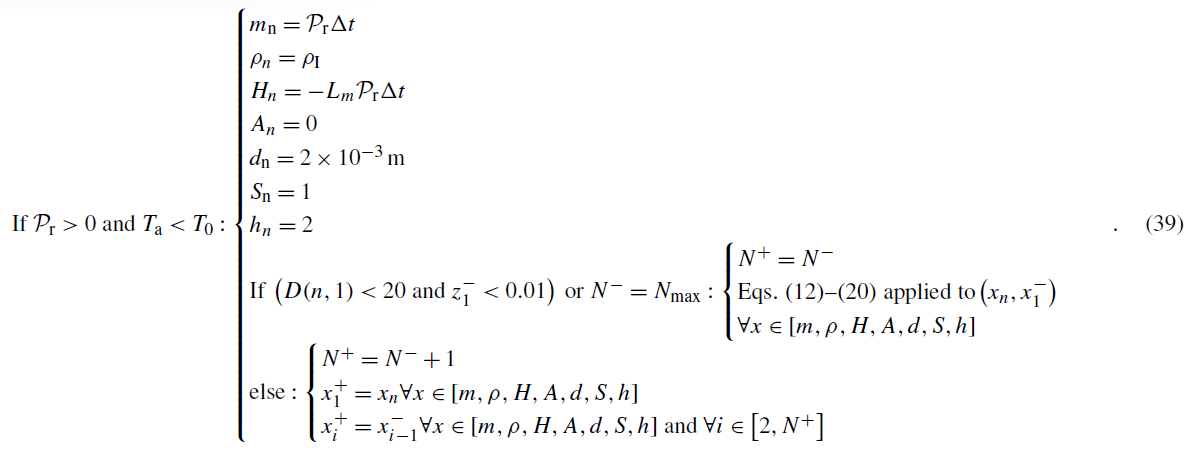

The energy associated with the phase change E_FRZ (W m⁻²) is computed by Eq. (40) and accounted for further as an additional energy source in the surface energy balance (Eq. 92), able to partly melt this new ice layer:

$$\begin{array}{}\text{(40)}& {\displaystyle }\left\{\begin{array}{ll}\mathrm{If}{\mathcal{P}}_{\mathrm{r}}>\mathrm{0}\mathrm{and}{T}_{\mathrm{a}}<T_{\mathrm{0}}:& E_{\mathrm{FRZ}}=\left(\mathrm{1}-{\mathit{\varphi }}_{\mathrm{FRZ}}\right)L_m{\mathcal{P}}_{\mathrm{r}}\mathrm{\Delta }t\mathrm{where}{\mathit{\varphi }}_{\mathrm{FRZ}}=\frac{c_{\mathrm{W}}}{L_m}\left(T_{\mathrm{0}}-T_{\mathrm{a}}\right)\\ \mathrm{else}:& E_{\mathrm{FRZ}}=\mathrm{0}\end{array}\right..\end{array}$$

The assumption behind Eq. (40) is that a fraction ϕ_FRZ of the latent heat release due to refreezing is consumed by the increase of temperature from T_a to T₀ and the remaining part is fully stored by the surface layer and can either be available for melting or be partly dissipated through diffusion or heat exchanges with the atmosphere, as solved later in Sect. 2.4.12 and 2.4.13.

Note that some other implementations of this process in other models consider than while all the precipitation eventually freezes and contributes to the formation of an ice layer at the surface, only a fraction of the associated latent heat is kept in the ice layer, while the remaining latent heat is transferred to the atmosphere at a shorter time scale than the model time step (Lackmann et al., 2002; Basnet and Thériault, 2025).

2.4.5 Metamorphism

The prognostic equations of microstructure variables d_i and S_i are still fully empirical in the absence of physical evolution laws. They depend on conditions of the vertical temperature gradient 𝒢_i estimated by:

$$\begin{array}{}\text{(41)}& \left\{\begin{array}{l}{\mathcal{G}}_{\mathrm{1}}=\frac{\mathrm{2}|T_{\mathrm{2}}-T_{\mathrm{1}}|}{z_{\mathrm{1}}+z_{\mathrm{2}}}\\ {\mathcal{G}}_i=\frac{\mathrm{2}|T_{i+\mathrm{1}}-T_{i-\mathrm{1}}|}{z_{i-\mathrm{1}}+\mathrm{2}{z}_i+z_{i+\mathrm{1}}}\forall i\in [\mathrm{2},N-\mathrm{1}]\\ {\mathcal{G}}_N=\frac{\mathrm{2}|T_N-T_{N-\mathrm{1}}|}{z_{N-\mathrm{1}}+z_N}\end{array}\right..\end{array}$$

Following Brun et al. (1992) and Vionnet et al. (2012), the evolution of sphericity ΔS_i during a time step Δ_t is defined by Eq. (42) (dry metamorphism) and Eq. (43) (wet metamorphism):

$$\begin{array}{}\text{(42)}& {\displaystyle }\mathrm{If}{l}_i=\mathrm{0}:& {\displaystyle }\left\{\begin{array}{ll}\mathrm{If}{\mathcal{G}}_i<\mathrm{5}\mathrm{K}{\mathrm{m}}^{-\mathrm{1}}& \left\{\begin{array}{ll}\mathrm{If}{S}_i<\mathrm{1}& \mathrm{\Delta }{S}_i={\mathrm{sph}}_{\mathrm{1}}{e}^{-\mathrm{6000}/T_i}{f}_{\mathrm{corr}}\left(d_i,S_i,h_i\right)\mathrm{\Delta }t\\ \mathrm{else}& \mathrm{\Delta }{S}_i=\mathrm{0}\end{array}\right.\\ \mathrm{else}& \left\{\begin{array}{ll}\mathrm{If}{S}_i>\mathrm{0}& \mathrm{\Delta }{S}_i=-{\mathrm{sph}}_{\mathrm{2}}{e}^{-\mathrm{6000}/T_i}{\mathcal{G}}_i^{\mathrm{0.4}}\mathrm{\Delta }t\\ \mathrm{else}& \mathrm{\Delta }{S}_i=\mathrm{0}\end{array}\right.\end{array}\right.\text{(43)}& {\displaystyle }\mathrm{If}{l}_i>\mathrm{0}:& {\displaystyle }\left\{\begin{array}{ll}\mathrm{If}{S}_i<\mathrm{1}:& \mathrm{\Delta }{S}_i=\max \left({\mathrm{sph}}_{\mathrm{3}}{\left(\mathrm{100}\frac{l_i}{{\mathit{\rho }}_i{z}_i}\right)}^{\mathrm{3}},{\mathrm{sph}}_{\mathrm{2}}{e}^{-\mathrm{6000}/T_{\mathrm{0}}}\right)\mathrm{\Delta }t\\ \mathrm{If}{S}_i=\mathrm{1}:& \mathrm{\Delta }{S}_i=\mathrm{0}\end{array}\right..\end{array}$$

Parameters sph₁, sph₂ and sph₃ are provided in Appendix K3. $f_{\mathrm{corr}}(d_i,S_i,h_i)$ is an unpublished parameterization in the original code of Vionnet et al. (2012) which modifies the general behaviour of Eq. (42) by reducing the sphericity increase of snow layers with microstructure properties typical of depth hoar or large faceted crystals and submitted to low thermal gradients. This prevents the formation of rounded grains from depth hoar or large faceted crystals. Indeed, the persistence of anisotropy in this case was obtained with a phase-field numerical model applied to snow microstructure (Bouvet et al., 2022) and recently confirmed by unpublished tomography observations.

$$\begin{array}{}\text{(44)}& {\displaystyle }\left\{\begin{array}{ll}\mathrm{If}{S}_i\ge \mathrm{0.5};h_i=\mathrm{1}\mathrm{and}{g}_{s_i}\left(d_i,S_i\right)>\mathrm{5}\times {\mathrm{10}}^{-\mathrm{4}}\mathrm{m}& f_{\mathrm{corr}}\left(d_i,S_i,h_i\right)=\mathrm{0}\\ \mathrm{If}{S}_i<\mathrm{0.5};h_i=\mathrm{1}\mathrm{and}{g}_{s_i}\left(d_i,S_i\right)>\mathrm{5}\times {\mathrm{10}}^{-\mathrm{4}}\mathrm{m}& f_{\mathrm{corr}}\left(d_i,S_i,h_i\right)=\exp \left(\frac{\mathrm{3}\times {\mathrm{10}}^{-\mathrm{4}}-g_{s_i}\left(d_i,S_i\right)}{{\mathrm{10}}^{-\mathrm{4}}}\right)\\ \mathrm{otherwise}& f_{\mathrm{corr}}\left(d_i,S_i,h_i\right)=\mathrm{1}\end{array}\right.\end{array}$$

h_i is a tracker of the snow layer history (Table 2) for which odd values (1, 3, 5) corresponds to the occurrence of depth hoar at any time since the layer creation. $g_{s_i}(d_i,S_i)$ is a variable originally used to describe snow microstructure by Brun et al. (1992) (grain size). Its retrieval from the current state variables d_i and S_i is described in Appendix D. It must be noticed that this parameterization was forgotten by Carmagnola et al. (2014) because it was unpublished and was only recently restored in the code.

Several prognostic evolutions of d_i during dry metamorphism were implemented by Carmagnola et al. (2014) and Lafaysse et al. (2017), following the works from Brun et al. (1992), Flanner and Zender (2006) and Schleef et al. (2014). Furthermore, several issues were found by Baron (2023) in the translation of the Brun et al. (1992) formalism (using dendricity and grain size) in terms of optical diameter evolution by Carmagnola et al. (2014) (details in Appendix D). A new parameterization (B21) was therefore recently implemented to solve the associated issues and now replaces the original implementation of Carmagnola et al. (2014) now removed from the code. The resulting available evolution laws of d_i during dry metamorphism are given by Eqs. (45)–(48).

$$\begin{array}{}\text{(45)}& {\displaystyle }\left[\begin{array}{r}{\displaystyle }\mathrm{If}\mathrm{SNOWMETAMO}=\mathrm{B}\mathrm{21}\\ {\displaystyle }\mathrm{and}{l}_i=\mathrm{0}:\end{array}\right]& {\displaystyle }\left\{\begin{array}{ll}\mathrm{If}{d}_i\ge {\mathrm{10}}^{-\mathrm{4}}\left(\mathrm{4}-S_i\right):& \left\{\begin{array}{ll}\mathrm{If}{\mathcal{G}}_i>\mathrm{15}\mathrm{K}{\mathrm{m}}^{-\mathrm{1}}\mathrm{and}{S}_i=\mathrm{0}:& \mathrm{\Delta }{d}_i=\frac{\mathrm{1}}{\mathrm{2}}f\left({\mathit{\theta }}_i\right)h\left({\mathit{\rho }}_i\right)g\left({\mathcal{G}}_i\right)\mathrm{\Phi }\mathrm{\Delta }t\\ \mathrm{else}:& \mathrm{\Delta }{d}_i=\frac{d_i-\mathrm{4}\times {\mathrm{10}}^{-\mathrm{4}}}{\mathrm{1}+S_i}\mathrm{\Delta }{S}_i\end{array}\right.\\ \mathrm{else}:& \mathrm{\Delta }{d}_i={\mathrm{10}}^{-\mathrm{4}}\left[-{\mathrm{sph}}_{\mathrm{2}}{e}^{-\mathrm{6000}/T_i}{\mathcal{J}}_i\left(S_i-\mathrm{3}\right)+\frac{\mathrm{\Delta }{S}_i}{\mathrm{\Delta }t}\frac{{\mathrm{10}}^{\mathrm{4}}{d}_i-\mathrm{1}}{S_i-\mathrm{3}}\right]\mathrm{\Delta }t\\ & \mathrm{where}\left\{\begin{array}{ll}{\mathcal{J}}_i={\mathcal{G}}_i^{\mathrm{0.4}}& \mathrm{if}{\mathcal{G}}_i\ge \mathrm{5}\\ {\mathcal{J}}_i=\mathrm{1}& \mathrm{if}{\mathcal{G}}_i<\mathrm{5}\end{array}\right.\end{array}\right.\text{(46)}& {\displaystyle }\left[\begin{array}{r}{\displaystyle }\mathrm{If}\mathrm{SNOWMETAMO}=\mathrm{F}\mathrm{06}\\ {\displaystyle }\mathrm{and}{l}_i=\mathrm{0}:\end{array}\right]& {\displaystyle }\mathrm{\Delta }{d}_i=\mathrm{2}{\dot{r}}_{\mathrm{0}}\left({\mathit{\rho }}_i,T_i,{\mathcal{G}}_i\right){\left[{\displaystyle \frac{\mathit{\tau }\left({\mathit{\rho }}_i,T_i,{\mathcal{G}}_i\right)}{\frac{d_i}{\mathrm{2}}-r_{\mathrm{0}}+\mathit{\tau }\left({\mathit{\rho }}_i,T_i,{\mathcal{G}}_i\right)}}\right]}^{\frac{\mathrm{1}}{\mathit{\kappa }\left({\mathit{\rho }}_i,T_i,{\mathcal{G}}_i\right)}}\mathrm{\Delta }t\text{(47)}& {\displaystyle }\left[\begin{array}{r}{\displaystyle }\mathrm{If}\mathrm{SNOWMETAMO}=\mathrm{S}\text{–}\mathrm{B}\\ {\displaystyle }\mathrm{and}{l}_i=\mathrm{0}:\end{array}\right]& {\displaystyle }\left\{\begin{array}{ll}\mathrm{If}{A}_i\le \mathrm{2}\mathrm{d}& \mathrm{\Delta }{d}_i=\frac{a_s{\mathit{\rho }}_i{d}_i^{\mathrm{2}}}{\mathrm{6}}+\frac{b_s{T}_i{\left(\frac{\mathrm{6}}{{\mathit{\rho }}_i}\right)}^{m_s-\mathrm{1}}}{d_i^{m_s-\mathrm{2}}}\\ \mathrm{else}:& \mathrm{Eq}.\left(\mathrm{46}\right)\end{array}\right.\text{(48)}& {\displaystyle }\left[\begin{array}{r}{\displaystyle }\mathrm{If}\mathrm{SNOWMETAMO}=\mathrm{S}\text{–}\mathrm{F}\\ {\displaystyle }\mathrm{and}{l}_i=\mathrm{0}:\end{array}\right]& {\displaystyle }\left\{\begin{array}{ll}\mathrm{If}{A}_i\le \mathrm{2}\mathrm{d}& \mathrm{Eq}.\left(\mathrm{48}\right)\\ \mathrm{else}:& \mathrm{Eq}.\left(\mathrm{47}\right)\end{array}\right..\end{array}$$

Functions f(θ_i), h(ρ_i), g(𝒢_i) and parameter Φ used in Eq. (45) for the growth of faceted crystals in the case of high gradient metamorphism follow Marbouty (1980) and are defined in Appendix C. In Eq. (46) from Flanner and Zender (2006), coefficients ${\dot{r}}_{\mathrm{0}}({\mathit{\rho }}_i,T_i,{\mathcal{G}}_i)$, $\mathit{\tau }({\mathit{\rho }}_i,T_i,{\mathcal{G}}_i)$ and $\mathit{\kappa }({\mathit{\rho }}_i,T_i,{\mathcal{G}}_i)$ are retrieved from look-up tables provided in a parameters file (cf. section on Data and Code availability) and $r_o=\mathrm{5}\times {\mathrm{10}}^{-\mathrm{5}}$ m. Experimental parameters a_s, b_s, m_s in Eq. (48) are defined in Appendix K3 from Schleef et al. (2014).

Regardless of the SNOWMETAMO option, wet metamorphism is always parameterized with the laws published by Vionnet et al. (2012), rewritten here with the new microstructure prognostic variables and the methodology described in Appendix D:

$$\begin{array}{}\text{(49)}& {\displaystyle }\mathrm{If}{l}_i>\mathrm{0}\left\{\begin{array}{l}\mathrm{If}{d}_i<{\mathrm{10}}^{-\mathrm{4}}\left(\mathrm{4}-S_i\right):\left\{\begin{array}{l}\mathrm{If}{S}_i<\mathrm{1}:\mathrm{\Delta }{d}_i={\mathrm{10}}^{-\mathrm{4}}\left(\frac{{\mathrm{10}}^{\mathrm{4}}{d}_i-\mathrm{1}}{S_i-\mathrm{3}}-(S_i-\mathrm{3})\right)\mathrm{\Delta }{S}_i\\ \mathrm{If}{S}_i=\mathrm{1}:\mathrm{\Delta }{d}_i={\mathrm{2.10}}^{-\mathrm{4}}\max \left({\mathrm{sph}}_{\mathrm{3}}{\left(\mathrm{100}\frac{l_i}{{\mathit{\rho }}_i{z}_i}\right)}^{\mathrm{3}},{\mathrm{sph}}_{\mathrm{2}}{e}^{-\mathrm{6000}/T_{\mathrm{0}}}\right)\mathrm{\Delta }t\end{array}\right.\\ \mathrm{else}:\left\{\begin{array}{l}\mathrm{If}{S}_i<\mathrm{1}:\mathrm{\Delta }{d}_i=\frac{d_i-{\mathrm{4.10}}^{-\mathrm{4}}}{S_i+\mathrm{1}}\mathrm{\Delta }{S}_i\\ \mathrm{If}{S}_i=\mathrm{1}:\mathrm{\Delta }{d}_i=\frac{\mathrm{2}}{\mathit{\pi }}\frac{\left[v_{\mathrm{0}}+v_{\mathrm{1}}{\left(\mathrm{100}\frac{l_i}{{\mathit{\rho }}_i{z}_i}\right)}^{\mathrm{3}}\right]}{d_i^{\mathrm{2}}}\mathrm{\Delta }t\end{array}\right.\end{array}\right..\end{array}$$

To follow its definition in Table 2, the historical tracker h_i is updated at the end of this subroutine by:

$$\begin{array}{}\text{(50)}& \left\{\begin{array}{l}\mathrm{If}{d}_i\ge {\mathrm{10}}^{-\mathrm{4}}\left(\mathrm{4}-S_i\right):\left\{\begin{array}{l}\mathrm{If}{S}_i=\mathrm{0}\mathrm{and}{h}_i^t=\mathrm{0}:h_i^{t+\mathrm{\Delta }t}=\mathrm{1}\\ \mathrm{else}:\left\{\begin{array}{l}\mathrm{If}{S}_i=\mathrm{1}\mathrm{and}\frac{l_i}{{\mathit{\rho }}_i{z}_i}>\mathrm{0.005}:\left\{\begin{array}{l}\mathrm{If}{h}_i^t=\mathrm{0}:h_i^{t+\mathrm{\Delta }t}=\mathrm{2}\\ \mathrm{If}{h}_i^t=\mathrm{1}:h_i^{t+\mathrm{\Delta }t}=\mathrm{3}\\ \mathrm{else}:h_i^{t+\mathrm{\Delta }t}=h_i^t\end{array}\right.\\ \mathrm{else}:\left\{\begin{array}{l}\mathrm{If}{T}_i<T_{\mathrm{0}}:\left\{\begin{array}{l}\mathrm{If}{h}_i^t=\mathrm{2}:h_i^{t+\mathrm{\Delta }t}=\mathrm{4}\\ \mathrm{If}{h}_i^t=\mathrm{3}:h_i^{t+\mathrm{\Delta }t}=\mathrm{5}\\ \mathrm{else}:h_i^{t+\mathrm{\Delta }t}=h_i^t\end{array}\right.\\ \mathrm{else}:h_i^{t+\mathrm{\Delta }t}=h_i^t\end{array}\right.\end{array}\right.\end{array}\right.\\ \mathrm{else}{h}_i^{t+\mathrm{\Delta }t}=h_i^t\end{array}\right..\end{array}$$

2.4.6 Natural compaction

For a given layer of density ρ_i the mechanical settling under the over burden σ_i (Pa) is expressed with a visco-elastic model (Anderson, 1976; Navarre, 1975):

$$\begin{array}{}\text{(51)}& \mathrm{If}\mathrm{SNOWCOMP}\in [\mathrm{B}\mathrm{92},\mathrm{T}\mathrm{11}]:\mathrm{\Delta }{\mathit{\rho }}_i={\displaystyle \frac{{\mathit{\rho }}_i{\mathit{\sigma }}_i}{{\mathit{\eta }}_i}}\mathrm{\Delta }t\end{array}$$

where

$$\begin{array}{}\text{(52)}& \left\{\begin{array}{l}{\mathit{\sigma }}_i=g\cos \mathrm{\Theta }{\sum }_{j=\mathrm{1}}^{i-\mathrm{1}}{\mathit{\rho }}_j{z}_j\forall i\in [\mathrm{2},N]\\ {\mathit{\sigma }}_{\mathrm{1}}=g\cos \mathrm{\Theta }\times \mathrm{0.5}{\mathit{\rho }}_{\mathrm{1}}{z}_{\mathrm{1}}\end{array}\right..\end{array}$$

g is the gravitational acceleration and Θ the slope angle from horizontal.

The viscosity η_i is a function of density ρ_i and temperature θ_i (°C) depending on the SNOWCOMP option (Lafaysse et al., 2017; Teufelsbauer, 2011):

$$\begin{array}{}\text{(53)}& \left\{\begin{array}{l}\mathrm{If}\mathrm{SNOWCOMP}=\mathrm{B}\mathrm{92}:{\mathit{\eta }}_i=f_{\mathrm{1}}\left(w_i\right)f_{\mathrm{2}}\left(d_i,S_i\right){\mathit{\eta }}_{\mathrm{0}}\frac{{\mathit{\rho }}_i}{c_{\mathit{\eta }}}{e}^{a_{\mathit{\eta }}\left(-{\mathit{\theta }}_i\right)+b_{\mathit{\eta }}{\mathit{\rho }}_i}\\ \mathrm{If}\mathrm{SNOWCOMP}=\mathrm{T}\mathrm{11}:{\mathit{\eta }}_i=f_{\mathrm{1}}\left(w_i\right)f_{\mathrm{2}}\left(d_i,S_i\right)\cdot \mathrm{0.05}{\mathit{\rho }}_i^{-\mathrm{0.0371}{\mathit{\theta }}_i+\mathrm{4.4}}\left({\mathrm{10}}^{-\mathrm{4}}{e}^{\mathrm{0.018}{\mathit{\rho }}_i}+\mathrm{1}\right)\end{array}\right..\end{array}$$

The parameters for case B92 are defined in Appendix K3. The multiplicative function f₁ accelerates the settlement of wet snow as a function of the volumetric liquid water content w_i. The multiplicative function f₂ reduces the settlement of layers consisting of faceted snow types as a function of microstructure properties d_i and S_i (translation of the formula from Vionnet et al., 2012 in the new formalism).

$$\begin{array}{}\text{(54)}& {\displaystyle }& {\displaystyle }{f}_{\mathrm{1}}\left(w_i\right)={\displaystyle \frac{\mathrm{1}}{\mathrm{1}+\mathrm{60}\frac{w_i}{{\mathit{\rho }}_{\mathrm{w}}}}}\text{(55)}& {\displaystyle }{f}_{\mathrm{2}}\left(d_i,S_i\right)& {\displaystyle }=\left\{\begin{array}{ll}\min \left(\mathrm{4},\exp \left(\min \left(\mathrm{4},g_{s_i}\left(d_i,S_i\right)\times {\mathrm{10}}^{\mathrm{4}}-\mathrm{2}\right)\right)\right)& \mathrm{if}{d}_i>\left(\mathrm{4}-S_i\right)\times {\mathrm{10}}^{-\mathrm{4}}\mathrm{and}{S}_i\le \mathrm{0.5}\\ \mathrm{1}& \mathrm{otherwise}\end{array}\right.\end{array}$$

where $g_{s_i}(d_i,S_i)$ is defined by Eq. (D6). The compaction rate however has a complex dependence on snow microstructure (Lehning et al., 2002) which cannot be described by the representation of snow microstructure in Crocus. Alternatively to Eq. (51), it is possible to use a parameterization from Schleef et al. (2014) derived from tomographic observations and representing a non-linear relationship between settlement, the stress σ_i (Pa) and the optical diameter increase for the first 48 hours after snowfall:

$$\begin{array}{}\text{(56)}& \mathrm{If}\mathrm{SNOWCOMP}=\mathrm{S}\mathrm{14}:\left\{\begin{array}{ll}\mathrm{\Delta }{\mathit{\rho }}_i=B_S\frac{\mathrm{\Delta }{d}_i}{d_i^{\mathrm{2}}}{\mathit{\sigma }}_i^{k_S}& \mathrm{if}{A}_i\le \mathrm{2}\mathrm{d}\\ \mathrm{Eq}.\left(\mathrm{53}\right)& \mathrm{if}{A}_i>\mathrm{2}\mathrm{days}\end{array}\right.\end{array}$$

with $B_S=\mathrm{3.96}\times {\mathrm{10}}^{-\mathrm{2}}$ and k_S=0.18. The current Crocus parameterization is applied when the snow layer age exceeds 2 d.

Alternative parameterizations reducing compaction in the presence of low vegetation were proposed by Woolley et al. (2024) combining earlier works from Domine et al. (2016) and Royer et al. (2021). Although not available in version 3.0.2, they will be implemented in a future version.

2.4.7 Grooming

The effects of grooming machines (snowcats) on the snow physical properties include the compaction induced by their overburden weight and the mixing of surface layers produced by the tiller. Both these effects can optionally be simulated in Crocus (Spandre et al., 2016).

The compaction effect is activated using the logical switch SNOWCOMPACT and only applies if the total mass $M=\sum _{i=\mathrm{1}}^N{m}_i$ is higher than 20 kg m⁻² (a minimum value required by the grooming machines) and between 20:00 and 21:00 LT (and also 06:00–09:00 LT in case of snowfall during the night). Grooming starts on 1 November and continues until the date day_END chosen by the user. Its frequency f_GRO (number of grooming sessions per day) is also user-defined. It is worth noticing that it is possible to activate grooming without activating snowmaking, but the opposite would not be realistic. The static stress due to the weight of the snowcat itself ${\mathit{\sigma }}_{{\mathrm{GRO}}_i}$ (Pa) is expressed for layer i by:

$$\begin{array}{}\text{(57)}& \mathrm{If}\mathrm{SNOWCOMPACT}\left\{\begin{array}{l}\mathrm{If}{\sum }_{j=\mathrm{1}}^i{m}_j<\mathrm{50}\mathrm{kg}{\mathrm{m}}^{-\mathrm{2}}:{\mathit{\sigma }}_{{\mathrm{GRO}}_i}=g\cos \mathrm{\Theta }\times \mathrm{500}\\ \mathrm{If}\mathrm{50}\mathrm{kg}{\mathrm{m}}^{-\mathrm{2}}\le {\sum }_{j=\mathrm{1}}^i{m}_j<\mathrm{150}\mathrm{kg}{\mathrm{m}}^{-\mathrm{2}}:{\mathit{\sigma }}_{{\mathrm{GRO}}_i}=g\cos \mathrm{\Theta }\times \left(\mathrm{150}-{\sum }_{j=\mathrm{1}}^i{m}_j\right)\cdot \mathrm{5}\\ \mathrm{If}{\sum }_{j=\mathrm{1}}^i{m}_j\ge \mathrm{150}\mathrm{kg}{\mathrm{m}}^{-\mathrm{2}}:{\mathit{\sigma }}_{{\mathrm{GRO}}_i}=\mathrm{0}\end{array}\right.\end{array}$$

and the corresponding density change is obtained by replacing σ_i by ${\mathit{\sigma }}_{{\mathrm{GRO}}_i}$ in Eq. (51).

The tilling effect is activated using the logical switch SNOWTILLER, applies down to 35 kg m⁻² below the surface and only if SNOWCOMPACT = True. The tiller mounted at the rear of snowcats produces two main effects: it further increases the density of the snow by loading the snowpack with extra pressure and it modifies the snow microstructure by creating smaller, rounded grains. As a result, all impacted layers are mixed together, their properties are homogenized and some of them are modified (Spandre et al., 2016). These effects are simulated in Crocus by directly modifying the density, optical diameter and sphericity of the impacted layers. The density reached by the snowpack after grooming is parameterized as:

$$\begin{array}{}\text{(58)}& \mathrm{If}\mathrm{SNOWTILLER}:{\mathit{\rho }}_i=\max \left(\stackrel{\mathrm{‾}}{\mathit{\rho }},{\displaystyle \frac{\mathrm{2}\stackrel{\mathrm{‾}}{\mathit{\rho }}+\mathrm{3}{\mathit{\rho }}_{\mathrm{GRO}}}{\mathrm{5}}}\right)\forall i\in [\mathrm{1},k]|\sum _{i=\mathrm{1}}^k{m}_i\le \mathrm{35}\mathrm{kg}{\mathrm{m}}^{-\mathrm{2}}\end{array}$$

where $\stackrel{\mathrm{‾}}{\mathit{\rho }}=\frac{\sum _{i=\mathrm{1}}^k{\mathit{\rho }}_i{m}_i}{\sum _{i=\mathrm{1}}^k{m}_i}$ is the weighted average density of the k impacted layers and ρ_GRO is the target density that should eventually be reached by the grooming process (Spandre et al., 2016; Hanzer et al., 2020). The optical diameter and sphericity of snow are altered analogously, using the respective target values d_GRO and S_GRO (Appendix K3, Spandre et al., 2016; Hanzer et al., 2020).

2.4.8 Drifting snow

Even if the Crocus model is not coupled with a dedicated module able to transport snow from one simulation point to another, it is possible to activate a parameterization from Vionnet et al. (2012) simulating the impact of drifting snow on compaction and metamorphism, but with mass conservation. This parameterization relies on two possible definitions of a mobility index MOB_i (Guyomarc'h and Merindol, 1998; Vionnet et al., 2012):

$$\begin{array}{}\text{(59)}& {\displaystyle }\left\{\begin{array}{ll}\mathrm{If}\mathrm{SNOWMOB}=\mathrm{GM}\mathrm{98}& \left\{\begin{array}{ll}\mathrm{If}{d}_i<{\mathrm{10}}^{-\mathrm{4}}\left(\mathrm{4}-S_i\right):& {\mathrm{MOB}}_i=\mathrm{0.5}\left(\mathrm{1}-S_i\right)+\mathrm{0.75}{\mathit{\delta }}_i\\ \mathrm{else}:& {\mathrm{MOB}}_i=\mathrm{0.833}\left(\mathrm{1}-S_i\right)-\mathrm{0.583}{g}_{s_i}\end{array}\right.\\ \mathrm{If}\mathrm{SNOWMOB}=\mathrm{VI}\mathrm{12}& \left\{\begin{array}{ll}\mathrm{If}{d}_i<{\mathrm{10}}^{-\mathrm{4}}\left(\mathrm{4}-S_i\right):& {\mathrm{MOB}}_i=\mathrm{0.34}\times \left(\mathrm{0.5}\left(\mathrm{1}-S_i\right)+\mathrm{0.75}{\mathit{\delta }}_i\right)+\mathrm{0.66}F\left({\mathit{\rho }}_i\right)\\ \mathrm{else}:& {\mathrm{MOB}}_i=\mathrm{0.34}\times \left(\mathrm{0.833}\left(\mathrm{1}-S_i\right)-\mathrm{0.583}{g}_{s_i}\right)+\mathrm{0.66}F\left({\mathit{\rho }}_i\right)\end{array}\right.\end{array}\right.\end{array}$$

where

$$\begin{array}{}\text{(60)}& F\left(\mathit{\rho }\right)=\left[\mathrm{1.25}-\mathrm{0.004}\left(\max \left({\mathit{\rho }}_{\min },\mathit{\rho }\right)-{\mathit{\rho }}_{\min }\right)\right]\mathrm{and}{\mathit{\rho }}_{\min }=\mathrm{50}\mathrm{kg}{\mathrm{m}}^{-\mathrm{3}}.\end{array}$$

In addition, a threshold is applied on the mobility index in case liquid water had been present at any time in the snow layer:

$$\begin{array}{}\text{(61)}& \mathrm{If}{h}_i\ge \mathrm{2}:{\mathrm{MOB}}_i=\min \left(-\mathrm{0.0583},{\mathrm{MOB}}_i\mathrm{from}\mathrm{Eq}.\mathrm{61}\right).\end{array}$$

The mobility index was expressed with the original formalism of metamorphism. The conversion functions δ_i(d_i,S_i) and $g_{s_i}(d_i,S_i)$ are defined in Appendix  refAmetamob21 by Eqs. (D2) and (D6). Redefining this index as a function of the current state variables (d_i and S_i) would be more consistent and flexible but it would require a significant new effort of evaluation. It highlights the issues involved by changes in the variable states in a model which have been underestimated in the work of Carmagnola et al. (2014).

A driftability index 𝒟_i is then obtained by combining the mobility index and the 5 m wind speed U₅:

$$\begin{array}{}\text{(62)}& {\mathcal{D}}_i=\max \left({\mathrm{MOB}}_i-\left(\mathrm{2.868}\cdot \exp \left(-\mathrm{0.085}\times U_{\mathrm{5}}\right)-\mathrm{1}.\right),\mathrm{0}\right).\end{array}$$

We then introduce:

$$\begin{array}{}\text{(63)}& {\mathcal{D}}_{{\mathrm{EFF}}_i}={\mathcal{D}}_i\times \exp \left(-\mathrm{10}\times \left(\sum _{j=\mathrm{1}}^{i-\mathrm{1}}{z}_j\left(\mathrm{3.25}-{\mathcal{D}}_j\right)+{\displaystyle \frac{z_i}{\mathrm{2}}}\left(\mathrm{3.25}-{\mathcal{D}}_i\right)\right)\right)\end{array}$$

to formulate the variation of density due to snow drift by:

$$\begin{array}{}\text{(64)}& \mathrm{\Delta }{\mathit{\rho }}_i={\mathcal{D}}_{{\mathrm{EFF}}_i}\max \left({\mathit{\rho }}_{\mathrm{MAX}}-{\mathit{\rho }}_i,\mathrm{0})\right){\displaystyle \frac{\mathrm{\Delta }t}{{\mathit{\tau }}_{\mathrm{DRIFT}}}}\end{array}$$

with ρ_MAX=350 kg m⁻³ and τ_DRIFT=172 800 s (2 d). Adjustments of parameters ρ_MAX and τ_DRIFT were proposed by several authors for Arctic snow as summarized by Woolley et al. (2024). Although hard-coded in version 3.0.2, they will be adjustable by the user in a future version. Then, the variation of microstructure properties due to fragmentation during snow transport are obtained by Eq. (65). The origin of this expression is provided in Appendix E.

$$\begin{array}{}\text{(65)}& {\displaystyle }\left\{\begin{array}{ll}\mathrm{If}{d}_i<{\mathrm{10}}^{-\mathrm{4}}\left(\mathrm{4}-S_i\right):& \mathrm{\Delta }{d}_i={\mathcal{D}}_{{\mathrm{EFF}}_i}\times {\mathrm{10}}^{-\mathrm{4}}\left[\left(\mathrm{2.5}-\mathrm{1.5}{S}_i\right){\mathit{\delta }}_i-\mathrm{1}+S_i\right]\frac{\mathrm{\Delta }t}{{\mathit{\tau }}_{\mathrm{DRIFT}}}\\ \mathrm{else}& \mathrm{\Delta }{d}_i={\mathcal{D}}_{{\mathrm{EFF}}_i}\left(-\mathrm{5}\times {\mathrm{10}}^{-\mathrm{4}}\frac{\mathrm{1}+S_i}{\mathrm{2}}+\left(d_i-\mathrm{4}\times {\mathrm{10}}^{-\mathrm{4}}\right)\frac{\mathrm{1}-S_i}{\mathrm{1}+S_i}\right)\frac{\mathrm{\Delta }t}{{\mathit{\tau }}_{\mathrm{DRIFT}}}\end{array}\right.\text{(66)}& {\displaystyle }\mathrm{\Delta }{S}_i={\mathcal{D}}_{{\mathrm{EFF}}_i}\left(\mathrm{1}-S_i\right){\displaystyle \frac{\mathrm{\Delta }t}{{\mathit{\tau }}_{\mathrm{DRIFT}}}}\end{array}$$

Optionally, a mass loss due to blowing snow sublimation can be estimated and removed from the surface layer. The parameterization is inspired from Gordon et al. (2006) with a modification of a threshold wind speed U_t to account for the microstructure-related mobility index. This option is not activated by default due to the large associated uncertainties and lack of evaluation but is considered to be necessary in polar environments (Brun et al., 2013; Woolley et al., 2024). The mass reduction of the surface layer due to sublimation Δm₁ is obtained by:

$$\begin{array}{}\text{(67)}& \mathrm{\Delta }{m}_{\mathrm{1}}=min\left(\mathrm{0.5}{m}_{\mathrm{1}},a_{\mathrm{SUBL}}{\left({\displaystyle \frac{T_{\mathrm{0}}}{T_{\mathrm{a}}}}\right)}^{{\mathit{\gamma }}_{\mathrm{SUBL}}}{U}_t{\mathit{\rho }}_{\mathrm{a}}{q}_{\mathrm{sat}}\left(T_{\mathrm{a}},P_{\mathrm{s}}\right)\left(\mathrm{1}-{\displaystyle \frac{q_{\mathrm{a}}}{q_{\mathrm{sat}}\left(T_{\mathrm{a}},P_{\mathrm{s}}\right)}}\right){\left({\displaystyle \frac{U_{\mathrm{5}}}{U_t}}\right)}^{b_{\mathrm{SUBL}}}\mathrm{\Delta }t\right)\end{array}$$

where

$$\begin{array}{}\text{(68)}& U_t={\displaystyle \frac{-\log \left(\frac{{\mathrm{MOB}}_{\mathrm{1}}+\mathrm{1}}{c_{\mathrm{SUBL}}}\right)}{d_{\mathrm{SUBL}}}}.\end{array}$$

The air density ρ_a (kg m⁻³) and the saturation specific humidity q_sat(T_a,P_s) (kg kg⁻¹) are computed following Appendix F. a_SUBL, b_SUBL, γ_SUBL, c_SUBL, d_SUBL are dimensionless parameters defined in Appendix K3.

2.4.9 Absorption of solar radiation

Two schemes of different complexities are currently implemented and can be activated through the SNOWRAD option. When SNOWRAD=B92, the initial 3-band scheme of Brun et al. (1992) is applied, inspired from Warren (1982). The incoming solar radiation at the interface between layers i and i+1 is defined by:

$$\begin{array}{}\text{(69)}& R_i=\sum _{k=\mathrm{1}}^{\mathrm{3}}\left(\mathrm{1}-{\mathit{\alpha }}_k\right){\mathit{\gamma }}_k\mathrm{SW}\downarrow \exp \left(-\sum _{j=\mathrm{1}}^i{\mathit{\beta }}_{k_j}{z}_j\right)\forall i\in [\mathrm{0},N]\mathrm{if}\mathrm{SNOWRAD}=\mathrm{B}\mathrm{92}.\end{array}$$

The spectral partitioning of incoming radiation is fixed by parameters γ_k (Appendix K3, with $\sum _{k=\mathrm{1}}^{\mathrm{3}}{\mathit{\gamma }}_k=\mathrm{1}$).

Spectral albedo values α_k are parameterized by:

$$\begin{array}{}\text{(70)}& {\mathit{\alpha }}_k=\mathit{\chi }{\mathit{\alpha }}_{k_{\mathrm{1}}}+(\mathrm{1}-\mathit{\chi }){\mathit{\alpha }}_{k_{\mathrm{2}}}\forall k\in [\mathrm{1},\mathrm{3}]\end{array}$$

where

$$\begin{array}{}\text{(71)}& {\displaystyle }\mathit{\chi }=\mathrm{0.8}\min \left(\mathrm{1},{\displaystyle \frac{z_{\mathrm{1}}}{\mathrm{0.02}}}\right)+\mathrm{0.2}\min \left[\mathrm{1},\max \left(\mathrm{0},{\displaystyle \frac{z_{\mathrm{1}}-\mathrm{0.02}}{\mathrm{0.01}}}\right)\right]\text{(72)}& {\displaystyle }\left\{\begin{array}{ll}{\mathit{\alpha }}_{{\mathrm{1}}_i}& =\max \left[\mathrm{0.6},\min \left(\mathrm{0.92},\mathrm{0.96}-\mathrm{1.58}\sqrt{d_i}\right)-\mathrm{0.2}\frac{A_i}{{\mathit{\tau }}_{\mathrm{a}}}\times \min \left(\max \left(\mathrm{0.5},\frac{P_{\mathrm{s}}}{P_{\mathrm{CDP}}}\right),\mathrm{1.5}\right)\right]\mathrm{if}{\mathit{\rho }}_i<{\mathit{\rho }}_{\mathrm{G}}\\ {\mathit{\alpha }}_{{\mathrm{1}}_i}& ={\mathit{\alpha }}_{{\mathrm{1}}_{\mathrm{G}}}\mathrm{if}{\mathit{\rho }}_i\ge {\mathit{\rho }}_{\mathrm{G}}\end{array}\right.\mathrm{for}i\in [\mathrm{1},\mathrm{2}]\text{(73)}& {\displaystyle }\left\{\begin{array}{ll}{\mathit{\alpha }}_{{\mathrm{2}}_i}& =\max \left(\mathrm{0.3},\mathrm{0.9}-\mathrm{15.4}\sqrt{d_i}\right)\mathrm{if}{\mathit{\rho }}_i<{\mathit{\rho }}_{\mathrm{G}}\\ {\mathit{\alpha }}_{{\mathrm{2}}_i}& ={\mathit{\alpha }}_{{\mathrm{2}}_{\mathrm{G}}}\mathrm{if}{\mathit{\rho }}_i\ge {\mathit{\rho }}_{\mathrm{G}}\end{array}\right.\mathrm{for}i\in [\mathrm{1},\mathrm{2}]\text{(74)}& {\displaystyle }\left\{\begin{array}{ll}{\mathit{\alpha }}_{{\mathrm{3}}_i}& =\mathrm{346.3}{d}_i^{\prime }-\mathrm{32.31}\sqrt{d_i^{\prime }}+\mathrm{0.88}\mathrm{if}{\mathit{\rho }}_i<{\mathit{\rho }}_{\mathrm{G}}\mathrm{where}{d}_i^{\prime }=\min \left(d_i,\mathrm{0.0023}\right)\\ {\mathit{\alpha }}_{{\mathrm{3}}_i}& ={\mathit{\alpha }}_{{\mathrm{3}}_{\mathrm{G}}}\mathrm{if}{\mathit{\rho }}_i\ge {\mathit{\rho }}_{\mathrm{G}}.\end{array}\right.\end{array}$$

Note that compared to Vionnet et al. (2012), the consideration of optical diameters of the first two layers, already in the code but not documented, is now made explicit in Eq. (70). The time constant τ_a in Eq. (72) is the main control of the parameterization reducing snow albedo in the visible band as a function of the age of the layer A_i in order to mimic the effect of Light-Absorbing Particles (LAP). Its default value is set to 60 d with an elevation-dependent multiplicative correction factor (function of P_s) assuming that LAP deposition decreases with elevation. However, it is recommended to adjust this parameter depending on the expected amount of LAP in the target region (Gaillard et al., 2025), to consider calibration against observed albedo time series when possible, or to apply several values of this parameter in multiphysics applications (Lafaysse et al., 2017). The last modification about absorption of solar radiation consists in applying constant glacier spectral albedo values ${\mathit{\alpha }}_{k_{\mathrm{G}}}$ on snow-free glacier surfaces. Default values (Appendix K5) are taken from Lejeune (2009) but must be adjusted to each specific glacier (e.g. Réveillet et al., 2018)

Absorption coefficients ${\mathit{\beta }}_{k_i}$ (m⁻¹) for band k and layer i are parameterized by:

$$\begin{array}{}\text{(75)}& {\displaystyle }& {\displaystyle }{\mathit{\beta }}_{{\mathrm{1}}_i}=\max \left(\mathrm{40},\mathrm{0.00192}{\displaystyle \frac{{\mathit{\rho }}_i}{\sqrt{d_i}}}\right)\forall i\in [\mathrm{1},N]\text{(76)}& {\displaystyle }& {\displaystyle }{\mathit{\beta }}_{{\mathrm{2}}_i}=\max \left(\mathrm{100},\mathrm{0.01098}{\displaystyle \frac{{\mathit{\rho }}_i}{\sqrt{d_i}}}\right)\forall i\in [\mathrm{1},N]\text{(77)}& {\displaystyle }& {\displaystyle }{\mathit{\beta }}_{{\mathrm{3}}_{\mathrm{1}}}=+\mathrm{\infty }.\end{array}$$

Alternatively to Eq. (69), an option is available for solar radiative transfer calculation in the snowpack (SNOWRAD = T17) combining the TARTES radiative scheme (Two-streAm Radiative TransfEr in Snow model, Picard and Libois, 2024) and an explicit modelling of LAP (Tuzet et al., 2017). TARTES is a two-stream radiative transfer scheme based on an analytical formulation of radiative transfer in snow (Kokhanovsky and Zege, 2004). The scheme is applied separately for the direct (DIR) and diffuse (DIF) components of solar radiation. For both components, TARTES computes spectral solar absorption within each layer $E_{k_i}$ (Eqs. 59–63 in the comprehensive scientific documentation of TARTES, Picard and Libois, 2024) and the spectral albedo α_k (Eq. 63 in Picard and Libois, 2024). Equation (78) is used to come back to the profile of R_i used in Crocus:

$$\begin{array}{}\text{(78)}& \begin{array}{rl}{R}_i=& \sum _{k=\mathrm{1}}^{N_k}\left(\left(\mathrm{1}-{\mathit{\alpha }}_{k\mathrm{DIR}}\right){\mathit{\gamma }}_{k\mathrm{DIR}}{\mathrm{SW}}_{\mathrm{DIR}}\downarrow -\sum _{j=\mathrm{1}}^i{E}_{k_j\mathrm{DIR}}+\left(\mathrm{1}-{\mathit{\alpha }}_{k\mathrm{DIF}}\right){\mathit{\gamma }}_{k\mathrm{DIF}}{\mathrm{SW}}_{\mathrm{DIF}}\downarrow -\sum _{j=\mathrm{1}}^i{E}_{k_j\mathrm{DIF}}\right)\\ & \forall i\in [\mathrm{0},N]\mathrm{if}\mathrm{SNOWRAD}=\mathrm{T}\mathrm{17}.\end{array}\end{array}$$

The default spectral resolution is 20 nm for N_k=111 spectral bands in the interval [300–2500 nm]. Coefficients γ_k DIR and γ_k DIF to split input direct and diffuse broadband radiation in spectral solar irradiance are currently provided as fixed parameters derived from SBDART (Ricchiazzi et al., 1998) under the conditions encountered at Col de Porte.

To compute $E_{k_i}$, TARTES accounts for the effect of snow physical properties (SSA and density) and Light-Absorbing Particles using the mass absorption efficiency of each LAP type and its mass content vertical profile. For dust, the mass absorption efficiency is defined following Eq. (83) of Picard and Libois (2024) with parameters λ₀=400 nm, MAE(λ₀)=110 m² kg⁻¹ and AAE=4.1 (values for dust PM_2.5 from Libya in Table 4 of Caponi et al., 2017). For black carbon, the mass absorption efficiency is defined following Eq. (82) of Picard and Libois (2024) with a constant density ρ_BC=1270 kg m⁻³ (Flanner et al., 2012) and a constant refractive index ($m_{\mathrm{BC}}=\mathrm{1.95}-\mathrm{0.79}i$ from Bond and Bergstrom, 2006). The MAE is then scaled with a multiplicative factor f_BC=1.638 to obtain an MAE value at 550 nm of 1.125×10⁴ m² kg⁻¹ consistently with measurements of Hadley and Kirchstetter (2012). The scaling makes it possible to implicitly account for the potential absorption enhancement due to internal particle mixing or particle coating. The implementation of new types of LAP would require the implementation of the description of their associated mass absorption efficiency. The vertical profile of LAP mass content is obtained following Sect. 2.4.10.

2.4.10 Light-absorbing particles

From Tuzet et al. (2017), the evolution law of the mass ℳ_i,j of LAP j in layer i is expressed as follows:

$$\begin{array}{}\text{(79)}& {\displaystyle }& {\displaystyle }{\mathcal{M}}_{\mathrm{1},j}^{+}={\mathcal{M}}_{\mathrm{1},j}^{-}+{\mathcal{W}}_{\mathrm{w},j}\mathrm{\Delta }t+{\displaystyle \frac{{\mathcal{W}}_{\mathrm{d},j}\mathrm{\Delta }t\exp \left(\frac{-z_{\mathrm{1}}}{h}\right)}{\sum _{k=\mathrm{1}}^N\exp \left(\frac{-Z_k}{h}\right)}}\text{(80)}& {\displaystyle }& {\displaystyle }{\mathcal{M}}_{i,j}^{+}={\mathcal{M}}_{i,j}^{-}+{\displaystyle \frac{{\mathcal{W}}_{\mathrm{d},j}\mathrm{\Delta }t\exp \left(\frac{-Z_i}{h}\right)}{\sum _{k=\mathrm{1}}^N\exp \left(\frac{-Z_k}{h}\right)}}\forall i\in [\mathrm{2},N]\end{array}$$

where Z_i represents the depth of layer i from the surface $\left(Z_i=\sum _{j=\mathrm{1}}^i{z}_j\right)$ and h the e-folding depth characterizing the decrease rate with depth of the impact of the dry deposition flux 𝒲_d,j. The wet deposition flux 𝒲_w,j only affects the uppermost layer.

However, in case of thin layers at the surface, a homogeneous repartition is applied on the uppermost N₁₀ layers gathering the first 10 kg m⁻² of snow. This limits artificial albedo variations due to vertical regridding (Dumont et al., 2020):

$$\begin{array}{}\text{(81)}& {\mathcal{M}}_{i,j}^{+}={\displaystyle \frac{m_i}{\sum _{k=\mathrm{1}}^{N_{\mathrm{10}}}{m}_k}}\times \sum _{k=\mathrm{1}}^{N_{\mathrm{10}}}{\mathcal{M}}_{k,j}^{+}\forall i\in \left[\mathrm{1},N_{\mathrm{10}}\right]\end{array}$$

where N₁₀ is the highest integer such that $\sum _{k=\mathrm{1}}^{N_{\mathrm{10}}-\mathrm{1}}{m}_k<\mathrm{10}$ kg m⁻².

Note than the wet deposition flux should be consistent with the occurrence of precipitation in the model input data. If not, any positive wet deposition flux without precipitation is not incorporated in the snowpack LAP mass content (Réveillet et al., 2022).

2.4.11 Turbulent fluxes

The sensible and latent turbulent heat fluxes are expressed by:

$$\begin{array}{}\text{(82)}& {\displaystyle }& {\displaystyle }H={\mathit{\rho }}_{\mathrm{a}}{c}_{\mathrm{P}}{C}_H{U}_{>\mathrm{1}}\left({\displaystyle \frac{T_{\mathrm{1}}}{{\mathrm{\Pi }}_{\mathrm{s}}}}-{\displaystyle \frac{T_{\mathrm{a}}}{{\mathrm{\Pi }}_{\mathrm{a}}}}\right)\text{(83)}& {\displaystyle }& {\displaystyle }LE={\mathit{\rho }}_{\mathrm{a}}{L}_{\mathrm{s}}{C}_H{U}_{>\mathrm{1}}\left(q_{\mathrm{sat}}\left(T_{\mathrm{1}},P_{\mathrm{s}}\right)-q_{\mathrm{a}}\right).\end{array}$$

ρ_a is the air volumetric mass (kg m⁻³), Π_s and Π_a the Exner functions at the surface and at the level of the atmospheric forcing and q_sat(T₁,P_s) the saturation specific humidity at surface temperature T₁ (kg kg⁻¹), cf. Appendix F for their computations. A minimum value of 1 m s⁻¹ is applied to wind speed ($U_{>\mathrm{1}}=\max (U,\mathrm{1}$ m s⁻¹)) to maintain minimal fluxes even with very low wind speeds. Note that a simplification has been introduced compared to Vionnet et al. (2012) by considering only surface sublimation and not evaporation of liquid water. The exchange coefficient C_H depends on the stability of the atmosphere through the Richardson Number Ri (Appendix F) following Noilhan and Mahfouf (1996):

$$\begin{array}{}\text{(84)}& \left\{\begin{array}{ll}{C}_H=\frac{{\mathit{\kappa }}_{\mathrm{VK}}^{\mathrm{2}}}{\ln \left(\frac{z_u}{z_{\mathrm{0}}}\right)\ln \left(\frac{z_{\mathrm{a}}}{z_{{\mathrm{0}}_{\mathrm{h}}}}\right)}\left(\mathrm{1}-\frac{\mathrm{15}Ri}{\mathrm{1}+C_h\sqrt{\left|Ri\right|}}\right)& \mathrm{if}Ri<=\mathrm{0}\\ C_H=\frac{{\mathit{\kappa }}_{\mathrm{VK}}^{\mathrm{2}}}{\ln \left(\frac{z_u}{z_{\mathrm{0}}}\right)\ln \left(\frac{z_{\mathrm{a}}}{z_{{\mathrm{0}}_{\mathrm{h}}}}\right)}\times \frac{\mathrm{1}}{\mathrm{1}+\mathrm{15}R{i}^{*}\sqrt{\mathrm{1}+\mathrm{5}R{i}^{*}}}& \mathrm{if}Ri>\mathrm{0}\mathrm{where}R{i}^{*}=\min \left(Ri,R{i}_l\right)\end{array}\right.\end{array}$$

where κ_VK is the Von Karman constant. Coefficient C_h in the unstable case is defined by:

$$\begin{array}{}\text{(85)}& C_h=\mathrm{15}\left(\mathrm{3.2165}+\mathrm{4.3431}\ln \left({\displaystyle \frac{z_{\mathrm{0}}}{z_{{\mathrm{0}}_{\mathrm{h}}}}}\right)+\mathrm{0.5360}{\left(\ln \left({\displaystyle \frac{z_{\mathrm{0}}}{z_{{\mathrm{0}}_{\mathrm{h}}}}}\right)\right)}^{\mathrm{2}}-\mathrm{0.0781}{\left(\ln \left({\displaystyle \frac{z_{\mathrm{0}}}{z_{{\mathrm{0}}_{\mathrm{h}}}}}\right)\right)}^{\mathrm{3}}\right){\displaystyle \frac{k^{\mathrm{2}}}{\ln \left(\frac{z_u}{z_{\mathrm{0}}}\right)\ln \left(\frac{z_{\mathrm{a}}}{z_{{\mathrm{0}}_{\mathrm{h}}}}\right)}}{\left({\displaystyle \frac{z_{\mathrm{a}}}{z_{{\mathrm{0}}_{\mathrm{h}}}}}\right)}^p\end{array}$$

where

$$\begin{array}{}\text{(86)}& p=\mathrm{0.5802}-\mathrm{0.1571}\ln \left({\displaystyle \frac{z_{\mathrm{0}}}{z_{{\mathrm{0}}_{\mathrm{h}}}}}\right)+\mathrm{0.0327}{\left(\ln \left({\displaystyle \frac{z_{\mathrm{0}}}{z_{{\mathrm{0}}_{\mathrm{h}}}}}\right)\right)}^{\mathrm{2}}-\mathrm{0.0026}{\left(\ln \left({\displaystyle \frac{z_{\mathrm{0}}}{z_{{\mathrm{0}}_{\mathrm{h}}}}}\right)\right)}^{\mathrm{3}}.\end{array}$$

In the stable case, an adjustable threshold Ri_l is applied on the Richardson number (Martin and Lejeune, 1998). Considering the high uncertainty of these parameterizations of turbulent processes, sensitivity analyses to momentum and thermodynamic roughness lengths z₀ and $z_{{\mathrm{0}}_{\mathrm{h}}}$  m) and to parameter Ri_l are recommended for robust applications of the model (Lafaysse et al., 2017).

2.4.12 Heat diffusion and energy balance

The formalism of this section is largely inspired by the documentation of the ISBA-ES (Explicit Snow) snowpack scheme from Boone (2002). The model solves the heat diffusion in the stratified snowpack using an implicit time integration scheme:

$$\begin{array}{}\text{(87)}& c_{\mathrm{I}}{\mathit{\rho }}_i{z}_i{\displaystyle \frac{T_i^{+}-T_i^{-}}{\mathrm{\Delta }t}}+E_i=G_{i-\mathrm{1}}^{+}-G_i^{+}\forall i\in [\mathrm{1},N]\end{array}$$

where $G_i^{+}$ (W m⁻²) represents the heat flux between layers i and $i+\mathrm{1}\forall i\in [\mathrm{1},N-\mathrm{1}]$ at the end of the time step. $G_{\mathrm{0}}^{+}$ and $G_N^{+}$ are the heat fluxes at the interfaces with atmosphere and soil at the end of the time step and E_i (W m⁻²) the energy of phase change for layer i. The main assumption of the model is that it is possible to separate heat diffusion and phase changes. Thus, the diffusion is solved assuming $E_i=\mathrm{0}\forall i\in [\mathrm{1},N]$.

The heat flux between two snow layers i and i+1 is the sum between the radiative flux R_i and the heat conduction $K_i^{+}$ (W m⁻²) between these layers:

$$\begin{array}{}\text{(88)}& G_i^{+}=K_i^{+}+R_i\forall i\in [\mathrm{1},N-\mathrm{1}].\end{array}$$

The conduction flux K_i is expressed at the end of the time step by:

$$\begin{array}{}\text{(89)}& K_i^{+}=\mathrm{2}\stackrel{\mathrm{‾}}{{\mathit{\lambda }}_i}{\displaystyle \frac{T_i^{+}-T_{i+\mathrm{1}}^{+}}{z_i+z_{i+\mathrm{1}}}}\forall i\in [\mathrm{1},N-\mathrm{1}]\end{array}$$

where $\stackrel{\mathrm{‾}}{{\mathit{\lambda }}_i}$ is the harmonic weighted mean of the thermal conductivities of layers i and i+1:

$$\begin{array}{}\text{(90)}& \stackrel{\mathrm{‾}}{{\mathit{\lambda }}_i}={\displaystyle \frac{z_i+z_{i+\mathrm{1}}}{\frac{z_i}{{\mathit{\lambda }}_i}+\frac{z_{i+\mathrm{1}}}{{\mathit{\lambda }}_{i+\mathrm{1}}}}}.\end{array}$$

Equation (90) replaces the arithmetic mean used in previous versions of Crocus (Lafaysse et al., 2025). Although there is not a clear agreement in the literature that harmonic means outperform the modelling of heat diffusion (Kadioglu et al., 2008), this solution is more consistent with the other components of SURFEX and more commonly used today in snow models (Fourteau et al., 2024).

The thermal conductivity λ_i of layer i is parameterized as a function of density ρ_i following parameterizations of Yen (1981), Calonne et al. (2011) or Boone and Etchevers (2001):

$$\begin{array}{}\text{(91)}& \left\{\begin{array}{ll}\mathrm{If}\mathrm{SNOWCOND}=\mathrm{Y}\mathrm{81}:& {\mathit{\lambda }}_i=\max \left[a_{\mathit{\lambda }}{\left(\frac{{\mathit{\rho }}_i}{{\mathit{\rho }}_{\mathrm{w}}}\right)}^{\mathrm{1.88}};{\mathit{\lambda }}_{\min }\right]\\ \mathrm{If}\mathrm{SNOWCOND}=\mathrm{C}\mathrm{11}:& {\mathit{\lambda }}_i=b_{\mathit{\lambda }}{\mathit{\rho }}_i^{\mathrm{2}}+c_{\mathit{\lambda }}{\mathit{\rho }}_i+d_{\mathit{\lambda }}\\ \mathrm{If}\mathrm{SNOWCOND}=\mathrm{I}\mathrm{02}:& {\mathit{\lambda }}_i=e_{\mathit{\lambda }}+f_{\mathit{\lambda }}{\mathit{\rho }}_i^{\mathrm{2}}+\left(g_{\mathit{\lambda }}+\frac{h_{\mathit{\lambda }}}{T_i^{-}+i_{\mathit{\lambda }}}\right)\frac{P_{\mathrm{0}}}{P}\end{array}\right..\end{array}$$

All empirical parameters are provided in Appendix K3. Alternatives to Eq. (91) were proposed by Woolley et al. (2024) for Arctic snow. Although not available in version 3.0.2, they will be implemented in a future version.

The heat flux between the atmosphere and the surface is the sum of all energy fluxes at the surface:

$$\begin{array}{}\text{(92)}& G_{\mathrm{0}}=R_{\mathrm{0}}+\mathit{ϵ}\left(\mathrm{LW}\downarrow -\mathit{\sigma }{T}_{\mathrm{1}}^{\mathrm{4}}\right)-H-LE+{\mathcal{P}}_{\mathrm{r}}\mathrm{\Delta }t\times c_{\mathrm{W}}\left(T_{\mathrm{a}}-T_{\mathrm{0}}\right)+E_{\mathrm{FRZ}}.\end{array}$$

All fluxes in Eq. (92) are expressed at time t+Δt with the following approximation:

$$\begin{array}{}\text{(93)}& F^{+}=F^{-}+{\displaystyle \frac{\partial F}{\partial T_{\mathrm{1}}}}\left(T_{\mathrm{1}}^{+}-T_{\mathrm{1}}^{-}\right).\end{array}$$

Thus,

$$\begin{array}{}\text{(94)}& \begin{array}{rl}{G}_{\mathrm{0}}^{+}=& R_{\mathrm{0}}+\mathit{ϵ}\left(\mathrm{LW}\downarrow -\mathit{\sigma }{\left(T_{\mathrm{1}}^{-}\right)}^{\mathrm{3}}\left(\mathrm{4}{T}_{\mathrm{1}}^{+}-\mathrm{3}{T}_{\mathrm{1}}^{-}\right)\right)-{\mathit{\rho }}_{\mathrm{a}}{c}_{\mathrm{P}}{C}_H{U}_{>\mathrm{1}}\left({\displaystyle \frac{T_{\mathrm{1}}^{+}}{{\mathrm{\Pi }}_{\mathrm{s}}}}-{\displaystyle \frac{T_{\mathrm{a}}}{{\mathrm{\Pi }}_{\mathrm{a}}}}\right)\\ & -{\mathit{\rho }}_{\mathrm{a}}{L}_{\mathrm{s}}{C}_H{U}_{>\mathrm{1}}\left(q_{\mathrm{sat}}\left(T_{\mathrm{1}}^{-},P_{\mathrm{s}}\right)-q_{\mathrm{a}}+{\displaystyle \frac{\partial q_{\mathrm{sat}}}{\partial T_{\mathrm{1}}}}\left(T_{\mathrm{1}}^{+}-T_{\mathrm{1}}^{-}\right)\right)+{\mathcal{P}}_{\mathrm{r}}\mathrm{\Delta }t\times c_{\mathrm{W}}\left(T_{\mathrm{a}}-T_{\mathrm{0}}\right)+E_{\mathrm{FRZ}}.\end{array}\end{array}$$

The computation of $\frac{\partial q_{\mathrm{sat}}}{\partial T_{\mathrm{1}}}$ is detailed in Appendix F. The heat flux between the bottom layer and the ground $G_N^{+}$ is expressed with a semi-implicit coupling (i.e. considering the ground surface temperature $T_{{\mathrm{G}}_{\mathrm{1}}}^{-}$ at time step t) in order to solve separately the thermal diffusion in the soil, outside the snowpack model:

$$\begin{array}{}\text{(95)}& G_N^{+}=\mathrm{2}\stackrel{\mathrm{‾}}{{\mathit{\lambda }}_N}{\displaystyle \frac{T_N^{+}-T_{{\mathrm{G}}_{\mathrm{1}}}^{-}}{z_N+z_{{\mathrm{G}}_{\mathrm{1}}}}}+R_N.\end{array}$$

where $\stackrel{\mathrm{‾}}{{\mathit{\lambda }}_N}$ is the harmonic mean between the thermal conductivity of the bottom snow layer λ_N and the thermal conductivity of the first soil layer ${\mathit{\lambda }}_{{\mathrm{G}}_{\mathrm{1}}}$:

$$\begin{array}{}\text{(96)}& \stackrel{\mathrm{‾}}{{\mathit{\lambda }}_N}={\displaystyle \frac{z_N+z_{{\mathrm{G}}_{\mathrm{1}}}}{\frac{z_N}{{\mathit{\lambda }}_N}+\frac{z_{{\mathrm{G}}_{\mathrm{1}}}}{{\mathit{\lambda }}_{{\mathrm{G}}_{\mathrm{1}}}}}}/\end{array}$$

Combining and rearranging Eqs. (87)–(89), (94) and (95) the system to solve becomes:

$$\begin{array}{}\text{(97)}& \left\{\begin{array}{l}\left\{\begin{array}{l}\left(\frac{c_{\mathrm{I}}{\mathit{\rho }}_{\mathrm{1}}{z}_{\mathrm{1}}}{\mathrm{\Delta }t}+\frac{\mathrm{2}\stackrel{\mathrm{‾}}{{\mathit{\lambda }}_{\mathrm{1}}}}{z_{\mathrm{1}}+z_{\mathrm{2}}}+\mathrm{4}\mathit{ϵ}\mathit{\sigma }{\left(T_{\mathrm{1}}^{-}\right)}^{\mathrm{3}}+{\mathit{\rho }}_{\mathrm{a}}{C}_H{U}_{>\mathrm{1}}\left(\frac{c_{\mathrm{P}}}{{\mathrm{\Pi }}_{\mathrm{s}}}+L_{\mathrm{s}}\frac{\partial q_{\mathrm{sat}}}{\partial T_{\mathrm{1}}}\right)\right)T_{\mathrm{1}}^{+}-\frac{\mathrm{2}\stackrel{\mathrm{‾}}{{\mathit{\lambda }}_{\mathrm{1}}}}{z_{\mathrm{1}}+z_{\mathrm{2}}}{T}_{\mathrm{2}}^{+}=\\ \frac{c_{\mathrm{I}}{\mathit{\rho }}_{\mathrm{1}}{z}_{\mathrm{1}}}{\mathrm{\Delta }t}{T}_{\mathrm{1}}^{-}+R_{\mathrm{0}}-R_{\mathrm{1}}+\mathit{ϵ}\left(\mathrm{LW}\downarrow +\mathrm{3}\mathit{\sigma }{\left(T_{\mathrm{1}}^{-}\right)}^{\mathrm{4}}\right)+{\mathit{\rho }}_{\mathrm{a}}{C}_H{U}_{>\mathrm{1}}\left(c_{\mathrm{P}}\frac{T_{\mathrm{a}}}{{\mathrm{\Pi }}_{\mathrm{a}}}+L_{\mathrm{s}}\left(q_{\mathrm{a}}-q_{\mathrm{sat}}\left(T_{\mathrm{1}}^{-},P_{\mathrm{s}}\right)+\frac{\partial q_{\mathrm{sat}}}{\partial T_{\mathrm{1}}}{T}_{\mathrm{1}}^{-}\right)\right)\\ +{\mathcal{P}}_{\mathrm{r}}\mathrm{\Delta }t\times c_{\mathrm{W}}\left(T_{\mathrm{a}}-T_{\mathrm{0}}\right)+E_{\mathrm{FRZ}}\end{array}\right.\\ -\frac{\mathrm{2}\stackrel{\mathrm{‾}}{{\mathit{\lambda }}_{i-\mathrm{1}}}}{z_{i-\mathrm{1}}+z_i}{T}_{i-\mathrm{1}}^{+}+\left(\frac{c_{\mathrm{I}}{\mathit{\rho }}_i{z}_i}{\mathrm{\Delta }t}+\frac{\mathrm{2}\stackrel{\mathrm{‾}}{{\mathit{\lambda }}_i}}{z_i+z_{i+\mathrm{1}}}+\frac{\mathrm{2}\stackrel{\mathrm{‾}}{{\mathit{\lambda }}_{i-\mathrm{1}}}}{z_{i-\mathrm{1}}+z_i}\right)T_i^{+}-\frac{\mathrm{2}\stackrel{\mathrm{‾}}{{\mathit{\lambda }}_i}}{z_i+z_{i+\mathrm{1}}}{T}_{i+\mathrm{1}}^{+}=\frac{c_{\mathrm{I}}{\mathit{\rho }}_i{z}_i}{\mathrm{\Delta }t}{T}_i^{-}+R_{i-\mathrm{1}}-R_i\forall i\in [\mathrm{2},N-\mathrm{1}]\\ -\frac{\mathrm{2}\stackrel{\mathrm{‾}}{{\mathit{\lambda }}_{N-\mathrm{1}}}}{z_{N-\mathrm{1}}+z_N}{T}_{N-\mathrm{1}}^{+}+\left(\frac{c_{\mathrm{I}}{\mathit{\rho }}_N{z}_N}{\mathrm{\Delta }t}+\frac{\mathrm{2}\stackrel{\mathrm{‾}}{{\mathit{\lambda }}_N}}{z_N+z_{{\mathrm{G}}_{\mathrm{1}}}}+\frac{\mathrm{2}\stackrel{\mathrm{‾}}{{\mathit{\lambda }}_{N-\mathrm{1}}}}{z_{N-\mathrm{1}}+z_N}\right)T_N^{+}=\frac{\mathrm{2}\stackrel{\mathrm{‾}}{{\mathit{\lambda }}_N}}{z_N+z_{{\mathrm{G}}_{\mathrm{1}}}}{T}_{{\mathrm{G}}_{\mathrm{1}}}^{-}+\frac{c_{\mathrm{I}}{\mathit{\rho }}_N{z}_N}{\mathrm{\Delta }t}{T}_N^{-}+R_{N-\mathrm{1}}-R_N.\end{array}\right.\end{array}$$

The first line of Eq. (97) is rewritten in the form:

$$\begin{array}{}\text{(98)}& {\displaystyle \frac{\mathrm{1}}{C_T\mathrm{\Delta }t}}{T}_{\mathrm{1}}^{+}-{\displaystyle \frac{{\mathit{\zeta }}_{\mathrm{2}}}{C_T\mathrm{\Delta }t}}{T}_{\mathrm{2}}^{+}={\displaystyle \frac{{\mathit{\zeta }}_{\mathrm{1}}}{C_T\mathrm{\Delta }t}}\end{array}$$

where

$$\begin{array}{}\text{(99)}& {\displaystyle }& {\displaystyle }{C}_T={\displaystyle \frac{\mathrm{1}}{c_{\mathrm{I}}{\mathit{\rho }}_{\mathrm{1}}{z}_{\mathrm{1}}}}\text{(100)}& {\displaystyle }& {\displaystyle }{\mathit{\zeta }}_{\mathrm{2}}={\displaystyle \frac{\mathrm{2}{C}_T\stackrel{\mathrm{‾}}{{\mathit{\lambda }}_{\mathrm{1}}}}{\mathcal{A}\left(z_{\mathrm{1}}+z_{\mathrm{2}}\right)}}\text{(101)}& {\displaystyle }& {\displaystyle }\mathcal{A}={\displaystyle \frac{\mathrm{1}}{\mathrm{\Delta }t}}+C_T\left[{\displaystyle \frac{\mathrm{2}\stackrel{\mathrm{‾}}{{\mathit{\lambda }}_{\mathrm{1}}}}{z_{\mathrm{1}}+z_{\mathrm{2}}}}+\mathrm{4}\mathit{ϵ}\mathit{\sigma }{\left(T_{\mathrm{1}}^{-}\right)}^{\mathrm{3}}+{\mathit{\rho }}_{\mathrm{a}}{C}_H{U}_{>\mathrm{1}}\left({\displaystyle \frac{c_{\mathrm{P}}}{{\mathrm{\Pi }}_{\mathrm{s}}}}+L_{\mathrm{s}}{\displaystyle \frac{\partial q_{\mathrm{sat}}}{\partial T_{\mathrm{1}}}}\right)\right]\text{(102)}& {\displaystyle }& {\displaystyle }{\mathit{\zeta }}_{\mathrm{1}}={\displaystyle \frac{\mathcal{B}{T}_{\mathrm{1}}^{-}+\mathcal{C}}{\mathcal{A}}}\text{(103)}& {\displaystyle }& {\displaystyle }\mathcal{B}={\displaystyle \frac{\mathrm{1}}{\mathrm{\Delta }t}}+C_T\left[\mathrm{3}\mathit{ϵ}\mathit{\sigma }{\left(T_{\mathrm{1}}^{-}\right)}^{\mathrm{3}}+{\mathit{\rho }}_{\mathrm{a}}{C}_H{U}_{>\mathrm{1}}{\displaystyle \frac{\partial q_{\mathrm{sat}}}{\partial T_{\mathrm{1}}}}\right]\text{(104)}& {\displaystyle }& {\displaystyle }\mathcal{C}=C_T\left[R_{\mathrm{0}}-R_{\mathrm{1}}+\mathit{ϵ}\mathrm{LW}\downarrow +{\mathit{\rho }}_{\mathrm{a}}{C}_H{U}_{>\mathrm{1}}\left(c_{\mathrm{P}}{\displaystyle \frac{T_{\mathrm{a}}}{{\mathrm{\Pi }}_{\mathrm{a}}}}+L_{\mathrm{s}}\left(q_{\mathrm{a}}-q_{\mathrm{sat}}\left(T_{\mathrm{1}}^{-},P_{\mathrm{s}}\right)\right)\right)+{\mathcal{P}}_{\mathrm{r}}\mathrm{\Delta }t\times c_{\mathrm{W}}\left(T_{\mathrm{a}}-T_{\mathrm{0}}\right)+E_{\mathrm{FRZ}}\right].\end{array}$$

Therefore, the temperature profile at time t+Δt is obtained by:

$$\begin{array}{}\text{(105)}& \left[\begin{array}{c}{T}_{\mathrm{1}}^{+}\\ T_{\mathrm{2}}^{+}\\ \mathrm{\dots }\\ T_i^{+}\\ \mathrm{\dots }\\ \mathrm{\dots }\\ T_N^{+}\end{array}\right]={\left[\begin{array}{ccccccc}{B}_{\mathrm{1}}& C_{\mathrm{1}}& \mathrm{0}& \mathrm{0}& \mathrm{\dots }& \mathrm{\dots }& \mathrm{0}\\ A_{\mathrm{2}}& B_{\mathrm{2}}& C_{\mathrm{2}}& \mathrm{0}& \mathrm{\dots }& \mathrm{\dots }& \mathrm{0}\\ \mathrm{0}& A_{\mathrm{3}}& \mathrm{\dots }& \mathrm{\dots }& \mathrm{\dots }& \mathrm{\dots }& \mathrm{\dots }\\ \mathrm{0}& \mathrm{0}& \mathrm{\dots }& B_i& C_i& \mathrm{\dots }& \mathrm{0}\\ \mathrm{\dots }& \mathrm{\dots }& \mathrm{\dots }& A_i& \mathrm{\dots }& \mathrm{\dots }& \mathrm{0}\\ \mathrm{\dots }& \mathrm{\dots }& \mathrm{\dots }& \mathrm{\dots }& \mathrm{\dots }& \mathrm{\dots }& C_{N-\mathrm{1}}\\ \mathrm{0}& \mathrm{0}& \mathrm{\dots }& \mathrm{0}& \mathrm{0}& A_N& B_N\end{array}\right]}^{-\mathrm{1}}\left[\begin{array}{c}{Y}_{\mathrm{1}}\\ Y_{\mathrm{2}}\\ \mathrm{\dots }\\ Y_i\\ \mathrm{\dots }\\ \mathrm{\dots }\\ Y_N\end{array}\right]\end{array}$$

where vectors $A=(A_{\mathrm{2}},\mathrm{\dots },A_i,\mathrm{\dots }{A}_N)$, $B=(B_{\mathrm{1}},\mathrm{\dots },B_i,\mathrm{\dots }{B}_N)$, $C=(C_{\mathrm{1}},\mathrm{\dots },C_i,\mathrm{\dots }{C}_{N-\mathrm{1}})$, $Y=(Y_{\mathrm{1}},\mathrm{\dots },Y_i,\mathrm{\dots }{Y}_N)$ are defined by:

$$\begin{array}{}\text{(106)}& \left\{\begin{array}{ll}{A}_i=& -\frac{\mathrm{2}\stackrel{\mathrm{‾}}{{\mathit{\lambda }}_{i-\mathrm{1}}}}{z_{i-\mathrm{1}}+z_i}\forall i\in [\mathrm{2},N]\\ B_{\mathrm{1}}=& \frac{\mathrm{1}}{C_T\mathrm{\Delta }t}\\ B_i=& \left(\frac{c_{\mathrm{I}}{\mathit{\rho }}_i{z}_i}{\mathrm{\Delta }t}+\frac{\mathrm{2}\stackrel{\mathrm{‾}}{{\mathit{\lambda }}_i}}{z_i+z_{i+\mathrm{1}}}+\frac{\mathrm{2}\stackrel{\mathrm{‾}}{{\mathit{\lambda }}_{i-\mathrm{1}}}}{z_{i-\mathrm{1}}+z_i}\right)\forall i\in [\mathrm{2},N-\mathrm{1}]\\ B_N=& \left(\frac{c_{\mathrm{I}}{\mathit{\rho }}_N{z}_N}{\mathrm{\Delta }t}+\frac{\mathrm{2}\stackrel{\mathrm{‾}}{{\mathit{\lambda }}_N}}{z_N+z_{{\mathrm{G}}_{\mathrm{1}}}}+\frac{\mathrm{2}\stackrel{\mathrm{‾}}{{\mathit{\lambda }}_{N-\mathrm{1}}}}{z_{N-\mathrm{1}}+z_N}\right)\\ C_{\mathrm{1}}=& -\frac{{\mathit{\zeta }}_{\mathrm{2}}}{C_T\mathrm{\Delta }t}\\ C_i=& -\frac{\mathrm{2}\stackrel{\mathrm{‾}}{{\mathit{\lambda }}_i}}{z_i+z_{i+\mathrm{1}}}\forall i\in [\mathrm{2},N-\mathrm{1}]\\ Y_{\mathrm{1}}=& \frac{{\mathit{\zeta }}_{\mathrm{1}}}{C_T\mathrm{\Delta }t}\\ Y_i=& \frac{c_{\mathrm{I}}{\mathit{\rho }}_i{z}_i}{\mathrm{\Delta }t}{T}_i^{-}+R_{i-\mathrm{1}}-R_i\forall i\in [\mathrm{2},N-\mathrm{1}]\\ Y_N=& \frac{\mathrm{2}\stackrel{\mathrm{‾}}{{\mathit{\lambda }}_N}}{z_N+z_{{\mathrm{G}}_{\mathrm{1}}}}{T}_{{\mathrm{G}}_{\mathrm{1}}}^{-}+\frac{c_{\mathrm{I}}{\mathit{\rho }}_N{z}_N}{\mathrm{\Delta }t}{T}_N^{-}+R_{N-\mathrm{1}}-R_N\end{array}\right..\end{array}$$

2.4.13 Adjustments in case of surface melting

The possibility for $T_{\mathrm{1}}^{+}$ to exceed the freezing point in the solving of Eq. (105) can lead to overestimate the surface energy fluxes that depend on $T_{\mathrm{1}}^{+}$ and to overestimate the heat conduction K₁ below surface. To avoid this numerical artefact, Crocus distinguishes the case of first melting ($T_{\mathrm{1}}^{-}<T_{\mathrm{0}}$ and $T_{\mathrm{1}}^{+}>T_{\mathrm{0}}$), and ongoing melting ($T_{\mathrm{1}}^{-}\ge T_{\mathrm{0}}$ and $T_{\mathrm{1}}^{+}>T_{\mathrm{0}}$).

In the case of a first melting ($T_{\mathrm{1}}^{-}<T_{\mathrm{0}}$ and $T_{\mathrm{1}}^{+}>T_{\mathrm{0}}$), the temperature profile for layers $i\in [\mathrm{2},N]$ is not updated, so only the surface fluxes are adjusted replacing $T_{\mathrm{1}}^{+}$ by T₀ in Eqs. (82), (83) and (94). The new temporary surface temperature (before melting) is obtained by converting the difference in both consecutive estimates of the surface energy flux G₀ in terms of temperature change:

$$\begin{array}{}\text{(107)}& \mathrm{If}{T}_{\mathrm{1}}^{-}<T_{\mathrm{0}}\mathrm{and}{T}_{\mathrm{1}}^{+}>T_{\mathrm{0}}:\left\{\begin{array}{ll}{G}_{\mathrm{0}}^{+}=& R_{\mathrm{0}}+\mathit{ϵ}\left(\mathrm{LW}\downarrow -\mathit{\sigma }{\left(T_{\mathrm{1}}^{-}\right)}^{\mathrm{3}}\left(\mathrm{4}{T}_{\mathrm{0}}-\mathrm{3}{T}_{\mathrm{1}}^{-}\right)\right)-{\mathit{\rho }}_{\mathrm{a}}{c}_{\mathrm{P}}{C}_H{U}_{>\mathrm{1}}\left(T_{\mathrm{0}}-T_{\mathrm{a}}\right)\\ & -{\mathit{\rho }}_{\mathrm{a}}{L}_{\mathrm{s}}{C}_H{U}_{>\mathrm{1}}\left(q_{\mathrm{sat}}\left(T_{\mathrm{1}}^{-},P_{\mathrm{s}}\right)-q_{\mathrm{a}}+\frac{\partial q_{\mathrm{sat}}}{\partial T_{\mathrm{0}}}\left(T_{\mathrm{0}}-T_{\mathrm{1}}^{-}\right)\right)+{\mathcal{P}}_{\mathrm{r}}\mathrm{\Delta }t\times c_{\mathrm{W}}\left(T_{\mathrm{a}}-T_{\mathrm{0}}\right)\\ T_{\mathrm{1}}^{+}=& T_{\mathrm{1}}^{\mathrm{first}}+\frac{\mathrm{\Delta }t}{c_{\mathrm{I}}{\mathit{\rho }}_i{z}_i}\left(G_{\mathrm{0}}^{+}-G_{\mathrm{0}}^{\mathrm{first}}\right)\end{array}\right.\end{array}$$

where $T_{\mathrm{1}}^{\mathrm{first}}$ is the solution of Eq. (105), and $G_{\mathrm{0}}^{\mathrm{first}}$ is the flux obtained applying Eq. (94) with $T_{\mathrm{1}}^{\mathrm{first}}$. This ensures that the energy budget over the snowpack is closed.

In the case of an ongoing melting (i.e. the solution of Eq. (105) provides a temperature above freezing point for the surface layer at two consecutive time steps: $T_{\mathrm{1}}^{-}\ge T_{\mathrm{0}}$ and $T_{\mathrm{1}}^{+}>T_{\mathrm{0}}$), the system is solved a second time for layers $i\in [\mathrm{2},N]$ by constraining $T_{\mathrm{1}}^{+}=T_{\mathrm{0}}$:

$$\begin{array}{}\text{(108)}& \left[\begin{array}{c}{T}_{\mathrm{2}}^{+}\\ \mathrm{\dots }\\ T_i^{+}\\ \mathrm{\dots }\\ \mathrm{\dots }\\ T_N^{+}\end{array}\right]={\left[\begin{array}{cccccc}{B}_{\mathrm{2}}& C_{\mathrm{2}}& \mathrm{0}& \mathrm{\dots }& \mathrm{\dots }& \mathrm{0}\\ A_{\mathrm{3}}& \mathrm{\dots }& \mathrm{\dots }& \mathrm{\dots }& \mathrm{\dots }& \mathrm{\dots }\\ \mathrm{0}& \mathrm{\dots }& B_i& C_i& \mathrm{\dots }& \mathrm{0}\\ \mathrm{\dots }& \mathrm{\dots }& A_i& \mathrm{\dots }& \mathrm{\dots }& \mathrm{0}\\ \mathrm{\dots }& \mathrm{\dots }& \mathrm{\dots }& \mathrm{\dots }& \mathrm{\dots }& C_{N-\mathrm{1}}\\ \mathrm{0}& \mathrm{\dots }& \mathrm{0}& \mathrm{0}& A_N& B_N\end{array}\right]}^{-\mathrm{1}}\left[\begin{array}{c}{Y}_{\mathrm{2}}+\frac{\mathrm{2}\stackrel{\mathrm{‾}}{{\mathit{\lambda }}_{\mathrm{1}}}}{z_{\mathrm{1}}+z_{\mathrm{2}}}{T}_{\mathrm{0}}\\ \mathrm{\dots }\\ Y_i\\ \mathrm{\dots }\\ \mathrm{\dots }\\ Y_N\end{array}\right].\end{array}$$

Then, the surface energy fluxes are updated replacing $T_{\mathrm{1}}^{+}$ and $T_{\mathrm{1}}^{-}$ by T₀ in Eqs. (82), (83), (94) and the conduction flux between the two first layers is updated with the solution of Eq. (108). A new estimate of the surface layer $T_{\mathrm{1}}^{+}$ is temporarily obtained from Eq. (87) (i=1) consistently with these updated fluxes, before the transfer of exceeding energy in phase change (E₁, see Sect. 2.4.16):

$$\begin{array}{}\text{(109)}& \mathrm{If}{T}_{\mathrm{1}}^{-}\ge T_{\mathrm{0}}\mathrm{and}{T}_{\mathrm{1}}^{+}>T_{\mathrm{0}}:\left\{\begin{array}{ll}{G}_{\mathrm{0}}^{+}=& R_{\mathrm{0}}+\mathit{ϵ}\left(\mathrm{LW}\downarrow -\mathit{\sigma }{T}_{\mathrm{0}}^{\mathrm{4}}\right)-{\mathit{\rho }}_{\mathrm{a}}{c}_{\mathrm{P}}{C}_H{U}_{>\mathrm{1}}\left(T_{\mathrm{0}}-T_{\mathrm{a}}\right)\\ & --{\mathit{\rho }}_{\mathrm{a}}{L}_{\mathrm{s}}{C}_H{U}_{>\mathrm{1}}\left(q_{\mathrm{sat}}\left(T_{\mathrm{0}},P_{\mathrm{s}}\right)-q_{\mathrm{a}}\right)+{\mathcal{P}}_{\mathrm{r}}\mathrm{\Delta }t\times c_{\mathrm{W}}\left(T_{\mathrm{a}}-T_{\mathrm{0}}\right)\\ K_{\mathrm{1}}^{+}=& \mathrm{2}\stackrel{\mathrm{‾}}{{\mathit{\lambda }}_i}\frac{T_{\mathrm{0}}-T_{\mathrm{2}}^{+}}{z_i+z_{i+\mathrm{1}}}\\ T_{\mathrm{1}}^{+}=& T_{\mathrm{0}}+\frac{\mathrm{\Delta }t}{c_{\mathrm{I}}{\mathit{\rho }}_i{z}_i}\left(G_{\mathrm{0}}^{+}-K_{\mathrm{1}}^{+}-R_{\mathrm{1}}\right)\end{array}\right..\end{array}$$

This also guarantees the closure of the energy budget in that case. Note that Fourteau et al. (2024) recently proposed alternative model formulations to compute a more stable surface energy balance with a better coupling between surface melting and heat transfers. This should be explored in the future to avoid the need of such numerical adjustments.

2.4.14 Coupling with MEB

MEB (Multiple Energy Balance, Boone et al., 2017) is a variant of the ISBA land surface scheme in which the soil-vegetation system is no longer described by a composite approach but by an explicit representation of vegetation with a big-leaf approach. This allows representation of the main physical processes involved in forest-snow interactions including snowfall interception and radiative impacts of the trees. An extensive description of this implementation is beyond the scope of this paper but available in Boone et al. (2017). However, as coupled processes require a coupled solving of snow surface and vegetation temperatures T₁ and T_v, the solving of heat diffusion is modified when Crocus is coupled to the MEB scheme. In that case, the values of the surface energy fluxes are no longer obtained through the implicit solving of Eqs. (97)–(105) but are imposed as a boundary condition to conserve energy. Equation (87) is modified for the surface layer to maintain the fluxes obtained from MEB:

$$\begin{array}{}\text{(110)}& c_{\mathrm{I}}{\mathit{\rho }}_i{z}_i{\displaystyle \frac{T_{\mathrm{1}}^{+}-T_{\mathrm{1}}^{-}}{\mathrm{\Delta }t}}+E_{\mathrm{1}}=G_{{\mathrm{0}}_{\mathrm{MEB}}}-R_{\mathrm{1}}-K_{\mathrm{1}}^{+}\end{array}$$

where

$$\begin{array}{}\text{(111)}& G_{{\mathrm{0}}_{\mathrm{MEB}}}=R_{\mathrm{0}}+\mathit{ϵ}\left(\mathrm{LW}\downarrow -\mathit{\sigma }{T}_{{\mathrm{1}}_{\mathrm{MEB}}}^{\mathrm{4}}\right)-H_{\mathrm{MEB}}-L{E}_{\mathrm{MEB}}+{\mathcal{P}}_{\mathrm{r}}\mathrm{\Delta }t\times c_{\mathrm{W}}\left(T_{\mathrm{a}}-T_{\mathrm{0}}\right).\end{array}$$

$G_{{\mathrm{0}}_{\mathrm{MEB}}}$ represents the total surface energy flux in agreement with the first estimate of surface temperature from MEB $T_{{\mathrm{1}}_{\mathrm{MEB}}}$ and the associated turbulent fluxes H_MEB and LE_MEB. LW↓ accounts for vegetation radiation and is therefore linked to the solution obtained for vegetation temperature $T_{{\mathrm{v}}_{\mathrm{MEB}}}$. It must be noted that as R₀ and R₁ are already needed in MEB, they are computed with the same routine as described in Secti. 2.4.9 but earlier in the time step (before the MEB solving) to guarantee identical values at both steps (MEB and Crocus), and accounting for shading by trees in SW↓.

Consistently with Eq. (110), the first line of Eq. (97) is replaced by:

$$\begin{array}{}\text{(112)}& \left({\displaystyle \frac{c_{\mathrm{I}}{\mathit{\rho }}_{\mathrm{1}}{z}_{\mathrm{1}}}{\mathrm{\Delta }t}}+{\displaystyle \frac{\mathrm{2}\stackrel{\mathrm{‾}}{{\mathit{\lambda }}_{\mathrm{1}}}}{z_{\mathrm{1}}+z_{\mathrm{2}}}}\right)T_{\mathrm{1}}^{+}-{\displaystyle \frac{\mathrm{2}\stackrel{\mathrm{‾}}{{\mathit{\lambda }}_{\mathrm{1}}}}{z_{\mathrm{1}}+z_{\mathrm{2}}}}{T}_{\mathrm{2}}^{+}={\displaystyle \frac{c_{\mathrm{I}}{\mathit{\rho }}_{\mathrm{1}}{z}_{\mathrm{1}}}{\mathrm{\Delta }t}}{T}_{\mathrm{1}}^{-}+G_{{\mathrm{0}}_{\text{MEB}}}-R_{\mathrm{1}}\end{array}$$

Rewriting Eq. (112) with the same form as Eq. (98) is equivalent to replacing Eqs. (101), (103) and (104) by Eqs. (113), (114), (115) and solving the linear system of Eq. (105) with coefficients C₁ and Y₁ of Eq. (106) modified according to the new values of ζ₂ and ζ₁ from Eqs. (100) and (102).

$$\begin{array}{}\text{(113)}& {\displaystyle }& {\displaystyle }\mathcal{A}={\displaystyle \frac{\mathrm{1}}{\mathrm{\Delta }t}}+C_T\left[{\displaystyle \frac{\mathrm{2}\stackrel{\mathrm{‾}}{{\mathit{\lambda }}_{\mathrm{1}}}}{z_{\mathrm{1}}+z_{\mathrm{2}}}}\right]\text{(114)}& {\displaystyle }& {\displaystyle }\mathcal{B}={\displaystyle \frac{\mathrm{1}}{\mathrm{\Delta }t}}\text{(115)}& {\displaystyle }& {\displaystyle }\mathcal{C}=C_T\left[G_{{\mathrm{0}}_{\mathrm{MEB}}}-R_{\mathrm{1}}\right]\end{array}$$

The adjustments of Sect. 2.4.13 are no longer required as G₀ is imposed by MEB and phase change was already accounted for to compute this flux.

The validity of Eq. (112) would require that no modification of the state variables of the snowpack has occurred between the computation of $G_{{\mathrm{0}}_{\mathrm{MEB}}}$ and the solving of Eq. (105) because $G_{{\mathrm{0}}_{\mathrm{MEB}}}$ depends on snow properties through Eqs. (48) and (49) in Boone et al. (2017) and the associated Appendix I4. In practice, the SURFEX code structure makes this constraint especially challenging. The violation of this assumption can generate numerical instabilities especially with thin surface layers due to the violation of the second principle of thermodynamics (Fourteau et al., 2026b). To reduce as much as possible the occurrence of this problem, the sequence of routines is modified following Fig. 1. However, there is currently no solution to avoid modifications due to snow interception by vegetation because this term cannot be computed before solving MEB (the mass balance depends on latent heat terms known only after the solving). Numerical instabilities are therefore still possible and further investigations are in progress to safely allow large scale applications of MEB-Crocus. This issue is more challenging than in the case of the coupling of MEB with ES snow scheme (Boone et al., 2017; Napoly et al., 2020) which has already been successfully applied in large scale simulations. This is probably due to the possible occurrence of thinner surface snow layers with Crocus.

2.4.15 Total melting or sublimation

The snowpack is assumed to totally disappear when

$$\begin{array}{}\text{(116)}& G_{\mathrm{0}}^{+}-G_N^{+}\ge {\displaystyle \frac{-\sum _{i=\mathrm{1}}^{N^t}{H}_i^{+}+H_{\mathrm{subl}}}{\mathrm{\Delta }t}}\mathrm{or}{\displaystyle \frac{\max \left(\mathrm{0},L{E}^{+}\right)\mathrm{\Delta }t}{L_{\mathrm{s}}}}\ge \sum _{i=\mathrm{1}}^{N^t}{m}_i.\end{array}$$

The first condition corresponds to a total melt of the snowpack (energy gain during the time step exceeds available internal energy for melting). It requires to remove the enthalpy of surface snow potentially sublimated H_subl from the total enthalpy. The second condition corresponds to a total sublimation of the snowpack, which is a very unusual case of snow disappearance but can appear especially when a snow transport module provide a very low amount of snow on bare ground in cold and windy conditions.

In both cases, for mass conservation, the runoff at the bottom of the snowpack is set to the total snow mass and the energy associated with LE⁺ is transmitted to the soil scheme as a correction term. If Eq. (116) is not verified, the procedure follows Sect. 2.4.16 to 2.4.20.

2.4.16 Melting

Let us define the mass of solid and liquid fractions of the snow before any phase change $s_i^{-}$ and $l_i^{-}$ (kg m⁻²):

$$\begin{array}{}\text{(117)}& s_i^{-}=m_i-l_i^{-}.\end{array}$$

When the heat diffusion solving provides a temperature $T_i^{+}$ above the melting point T₀ for layer i, the model simulates melting. The energy available for fusion $E_{{\mathrm{f}}_i}$ (J m⁻²) on layer i can be constrained either by the available heating energy or by the available mass of the solid fraction of snow before melting $s_i^{-}$. Thus, the energy and mass f_i (kg m⁻²) of melting during the time step are computed by:

$$\begin{array}{}\text{(118)}& {\displaystyle }& {\displaystyle }{E}_{{\mathrm{f}}_i}=\min \left(c_{\mathrm{I}}{\mathit{\rho }}_i\left(T_i^{+}-T_{\mathrm{0}}\right),L_m{s}_i^{-}\right)\text{(119)}& {\displaystyle }& {\displaystyle }{f}_i={\displaystyle \frac{E_{{\mathrm{f}}_i}}{L_m}}.\end{array}$$

The mass of solid and liquid fractions after melting are:

$$\begin{array}{}\text{(120)}& {\displaystyle }& {\displaystyle }{s}_i^{+}=s_i^{-}-f_i\text{(121)}& {\displaystyle }& {\displaystyle }{l}_i^{+}=l_i^{-}+f_i\end{array}$$

The corresponding updates of depth and total density can be expressed by:

$$\begin{array}{}\text{(122)}& {\displaystyle }& {\displaystyle }{z}_i^{+}=z_i^{-}\times {\displaystyle \frac{m_i-l_i^{+}}{m_i-l_i^{-}}}\text{(123)}& {\displaystyle }& {\displaystyle }{\mathit{\rho }}_i^{+}={\displaystyle \frac{m_i}{z_i^{+}}}.\end{array}$$

In case of melting, the melting point temperature is attributed to the layer temperature:

$$\begin{array}{}\text{(124)}& T_i^{++}=\min \left(T_{\mathrm{0}},T_i^{+}\right).\end{array}$$

In practice, a first evaluation of Eqs. (118)–(119) is computed for all layers to identify cases where a numerical layer fully melts out ($c_{\mathrm{I}}{\mathit{\rho }}_i(T_i^{+}-T_{\mathrm{0}})\ge L_m{s}_i^{-}$). In such a case, the numerical layer i is aggregated with the numerical layer i+1 for $i\in [\mathrm{1},N-\mathrm{1}]$, following Eqs. (12)–(20). If the bottom layer N is concerned, it is agregated with the above layer N−1. Several iterations can be done in case of melting of multiple consecutive layers. Then, the melting is computed again with this updated discretization with the guarantee that all numerical layers remain defined.

2.4.17 Refreezing

When the heat diffusion solving provides a temperature $T_i^{+}$ below the melting point T₀ whereas liquid water is present, the model simulates refreezing. The energy available for refreezing $E_{{\mathrm{r}}_i}$ (J m⁻²) can be constrained either by the layer cooling after diffusion or by the maximum available liquid water content before refreezing $l_i^{-}$. Thus, the energy and mass r_i (kg m⁻²) of refreezing during the time step are computed by:

$$\begin{array}{}\text{(125)}& {\displaystyle }& {\displaystyle }{E}_{{\mathrm{r}}_i}=\min \left(c_{\mathrm{I}}{\mathit{\rho }}_i\left(T_{\mathrm{0}}-T_i^{+}\right),L_m{l}_i^{-}\right)\text{(126)}& {\displaystyle }& {\displaystyle }{r}_i={\displaystyle \frac{E_{{\mathrm{r}}_i}}{L_m}}.\end{array}$$

The mass of solid and liquid fractions after refreezing are:

$$\begin{array}{}\text{(127)}& {\displaystyle }& {\displaystyle }{s}_i^{+}=s_i^{-}+r_i\text{(128)}& {\displaystyle }& {\displaystyle }{l}_i^{+}=l_i^{-}-r_i.\end{array}$$

The energy conservation during the refreezing process is expressed by:

$$\begin{array}{}\text{(129)}& c_{\mathrm{I}}{\mathit{\rho }}_i\left(T_i^{+}-T_i^{++}\right)s_i^{+}+E_{{\mathrm{r}}_i}+c_{\mathrm{I}}{\mathit{\rho }}_i\left(T_{\mathrm{0}}-T_i^{+}\right)r_i=\mathrm{0}\end{array}$$

where $T_i^{+}$ and $T_i^{++}$ (K) are the layer temperature of the solid fraction before and after refreezing. In Eq. (129), the first term corresponds to the heating of the solid fraction after refreezing, the second term to the latent heat release due to refreezing and the third term to the cooling of the refrozen part necessary for the thermal equilibrium of the solid phase.

By combining Eqs. (129) and (128), the evolution of the layer temperature due to refreezing is computed by:

$$\begin{array}{}\text{(130)}& T_i^{++}=T_{\mathrm{0}}+\left(T_i^{+}-T_{\mathrm{0}}\right){\displaystyle \frac{s_i^{-}}{s_i^{+}}}+{\displaystyle \frac{E_{{\mathrm{r}}_i}}{c_{\mathrm{I}}{\mathit{\rho }}_i{s}_i^{+}}}.\end{array}$$

Equations (125)–(130) are not applied independently but jointly with liquid water percolation as described in Sect. 2.4.18 within Algorithm 1.

Algorithm 1 Buckets algorithm for liquid water percolation.

ℱ₀=𝒫_rΔt

for $i\in [\mathrm{1},N]$ do

Compute r_i, s_i, w_i with Eqs. (127)–(133)

$w_i^{*}=w_i+\frac{{\mathcal{F}}_{i-\mathrm{1}}+f_i-r_i}{z_i}$

${\mathcal{F}}_i=\max (\mathrm{0},w_i^{*}-w_{i\max })z_i$

$w_i=w_i^{*}-\frac{{\mathcal{F}}_i}{z_i}$

${\mathit{\rho }}_i^{+}={\mathit{\rho }}_i^{-}({\mathcal{F}}_i-{\mathcal{F}}_{i-\mathrm{1}})\frac{{\mathit{\rho }}_W}{z_i}$

if ${\mathit{\rho }}_i^{+}>{\mathit{\rho }}_{\mathrm{I}}$ then

$z_i=\frac{{\mathit{\rho }}_i^{+}}{{\mathit{\rho }}_{\mathrm{I}}}{z}_i$

${\mathit{\rho }}_i^{+}={\mathit{\rho }}_{\mathrm{I}}$

end if

end for

2.4.18 Liquid water percolation

Let us define the volumetric liquid water content w_i (kg m⁻³):

$$\begin{array}{}\text{(131)}& w_i={\displaystyle \frac{l_i}{z_i}}\end{array}$$

and the snow porosity:

$$\begin{array}{}\text{(132)}& {\mathit{\varphi }}_i=\mathrm{1}-{\displaystyle \frac{{\mathit{\rho }}_i^{-}-w_i}{{\mathit{\rho }}_{\mathrm{I}}}}\end{array}$$

where ρ_I is the volumetric mass of pure ice. The liquid water flow ℱ_i (kg m⁻²) between layers i and i+1 is computed by a simple and conceptual bucket approach where the layers are seen as superposed water reservoirs with a maximum liquid water holding capacity w_i max. The excess water drains to the underlying layer when w_i exceeds w_i max following Algorithm 1. Snow layer densities ρ_i are updated with the resulting net mass flux ${\mathcal{F}}_i-{\mathcal{F}}_{i-\mathrm{1}}$. However, in the limit case of ice layers (ρ=ρ_I) and refreezing (r_i>0), the excess liquid water mass increases the ice layer depth at constant density. Note that another choice would be possible (Fourteau et al., 2024) by considering ice layers impermeable (i.e. computing ℱ_i before any refreezing and r_i after percolation) with potential impacts on glaciers simulations.

Several formulations of w_i max were implemented by Lafaysse et al. (2017):

$$\begin{array}{}\text{(133)}& \left\{\begin{array}{l}\mathrm{If}\mathrm{SNOWLIQ}=\mathrm{B}\mathrm{92}:w_{i\max }=\mathrm{0.05}{\mathit{\rho }}_{\mathrm{w}}{\mathit{\varphi }}_i\\ \mathrm{If}\mathrm{SNOWLIQ}=\mathrm{SPK}:\left\{\begin{array}{ll}{w}_{i\max }={\mathit{\rho }}_{\mathrm{w}}\left(\mathrm{0.08}-\mathrm{0.1023}\left(\mathrm{0.97}-{\mathit{\varphi }}_i\right)\right)& \mathrm{if}{\mathit{\varphi }}_i\ge \mathrm{0.77}\\ w_{i\max }={\mathit{\rho }}_{\mathrm{w}}\left(\mathrm{0.0264}+\mathrm{0.0099}\frac{{\mathit{\varphi }}_i}{\mathrm{1}-{\mathit{\varphi }}_i}\right)& \mathrm{otherwise}\end{array}\right.\\ \mathrm{If}\mathrm{SNOWLIQ}=\mathrm{B}\mathrm{02}:w_{i\max }={\mathit{\rho }}_i\left(r_{\min }+\left(r_{\max }-r_{\min }\right)\max \left(\mathrm{0},\frac{{\mathit{\rho }}_r-{\mathit{\rho }}_i}{{\mathit{\rho }}_r}\right)\right)\end{array}\right..\end{array}$$

Parameters r_min, r_max ρ_r are defined in Appendix K3.

The resolution of Richards equations might help improve the realism of this process in a detailed snowpack model (Wever et al., 2014, 2015, 2016a, b, 2017). However, the developments of D'Amboise et al. (2017) are not sufficiently robust to be available in this official release. More stable and numerically efficient alternatives are emerging and might be preferred in the future following the recommendations of Fourteau et al. (2026a).

2.4.19 Scavenging of LAP

When LAP are activated (Sect. 2.4.10), liquid water percolation may carry a fraction of LAP mass (Tuzet et al., 2017):

$$\begin{array}{}\text{(134)}& {\mathcal{M}}_{i,j}^{+}={\mathcal{M}}_{i,j}^{-}-{\mathcal{F}}_i\times C_{\mathrm{scav},j}\times {\displaystyle \frac{{\mathcal{M}}_{i,j}^{-}}{m_i}}.\end{array}$$

The scavenging coefficient C_scav,j can be adjusted by the user for each LAP j (default values are set to $C_{\mathrm{scav},j}=\mathrm{0}$ i.e. no scavenging).

2.4.20 Sublimation and deposition

Sublimation and deposition are accounted for by adding or removing mass to the surface layer accordingly with the surface latent heat flux (Eq. 83 where T₁ is the solution of Eqs. (105), (107) or (109) depending on the occurrence of melting). The corresponding evolution of the surface layer properties is described by Eqs. (135)–(136).

$$\begin{array}{}\text{(135)}& {\displaystyle }& {\displaystyle }{z}_{\mathrm{1}}^{+}=\max \left(z_{\mathrm{1}}+LE{\displaystyle \frac{\mathrm{\Delta }t}{L_{\mathrm{s}}\left({\mathit{\rho }}_{\mathrm{1}}^{-}-\frac{l_{\mathrm{1}}}{z_{\mathrm{1}}^{-}}\right)}},\mathrm{0}\right)\text{(136)}& {\displaystyle }& {\displaystyle }{\mathit{\rho }}_{\mathrm{1}}^{+}={\mathit{\rho }}_{\mathrm{1}}^{-}+{\displaystyle \frac{l_{\mathrm{1}}}{z_{\mathrm{1}}^{+}}}.\end{array}$$

Microstructure properties are not modified. Therefore, in case of deposition, the current Crocus snow model only increases the mass of the surface snow layer but it does not allow the formation of a dedicated layer with microstructure properties typical of surface hoar. As a result, it is neither possible to track the burying of surface hoar in the snowpack. In the very unusual cases when the mass of the surface layer is insufficient for sublimation $\left(-LE\frac{\mathrm{\Delta }t}{L_{\mathrm{s}}}>z_i\left({\mathit{\rho }}_i^{-}-\frac{l_i}{z_i^{-}}\right)\right)$ which only occurs for extremely thin snowpacks), the quantity $-LE\frac{\mathrm{\Delta }t}{L_{\mathrm{s}}}-z_i\left({\mathit{\rho }}_i^{-}-\frac{l_i}{z_i^{-}}\right)$ is later extracted from the first soil layer in the ISBA-DIF soil scheme to conserve energy, and the remaining liquid water, if any, is transferred to the next layer. A homogeneous regridding is applied before the next time step.

2.4.21 Unloading from vegetation

In case of unloading from vegetation, the initial implementation of MEB consisted in adding the unloaded mass to the mass of solid precipitation m_SP, following Eqs. (35) and (36) for snow density and microstructure. This could lead to unrealistic surface density when unloading occurred in cold conditions. A recent new parameterization instead attributes a fixed density ρ_UN and microstructure properties d_UN and S_UN to unloaded snow. The associated snow mass is either aggregated to the surface snow layer following Eqs. (12)–(20) or associated to a new snow layer depending on the properties of the surface snow layer.

3 Diagnoses

This section describes the complementary diagnoses of a Crocus simulation provided in addition to the state variables of the model. These diagnoses can be useful for model evaluation or interpretation in research or operational applications.

3.1 Diagnoses of recent, wet or refrozen snow

We define n_X as the number of snow layers more recent than X days, i.e. satisfying the following condition:

$$\begin{array}{}\text{(137)}& A_i<X\forall i\in \left[\mathrm{1},n_X\right].\end{array}$$

Thus, thickness Z_X and mass M_X of snow more recent than X days are defined by:

$$\begin{array}{}\text{(138)}& {\displaystyle }& {\displaystyle }{Z}_X=\sum _{i=\mathrm{1}}^{n_X}{z}_i\text{(139)}& {\displaystyle }& {\displaystyle }{M}_X=\sum _{i=\mathrm{1}}^{n_X}{m}_i.\end{array}$$

These diagnoses are provided for $X\in [\mathrm{0.5},\mathrm{1},\mathrm{3},\mathrm{5},\mathrm{7}]$. Similarly, the number of wet and refrozen snow layers from the surface n_w and n_r are defined by:

$$\begin{array}{}\text{(140)}& {\displaystyle }& {\displaystyle }{l}_i>\mathrm{0}\forall i\in \left[\mathrm{1},n_{\mathrm{w}}\right]\text{(141)}& {\displaystyle }& {\displaystyle }{l}_i<\mathrm{0}\forall i\in \left[\mathrm{1},n_{\mathrm{r}}\right].\end{array}$$

The thickness of wet and refrozen snow Z_w and Z_r are diagnosed by:

$$\begin{array}{}\text{(142)}& {\displaystyle }& {\displaystyle }{Z}_{\mathrm{w}}=\sum _{i=\mathrm{1}}^{n_{\mathrm{w}}}{z}_i\text{(143)}& {\displaystyle }& {\displaystyle }{Z}_{\mathrm{r}}=\sum _{i=\mathrm{1}}^{n_{\mathrm{r}}}{z}_i.\end{array}$$

3.2 Grain type classification

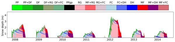
For each snow layer, a diagnosis of grain type Ψ_i is derived from values of optical diameter and sphericity through the following classification (Eq. 144) in which δ_i(d_i,S_i) and $g_{{\mathrm{s}}_i}(d_i,S_i)$ are defined respectively by Eqs. (D2) and (D6). The values taken by Ψ_i are taken from the International Snow Classification (Fierz et al., 2009) and include PP (Precipitation Particles), D (Depth Hoars), MF (Melt Forms) and combinations of these types.

$$\begin{array}{}\text{(144)}& {\displaystyle }\left\{\begin{array}{ll}\mathrm{If}{d}_i<{\mathrm{10}}^{-\mathrm{4}}\left(\mathrm{4}-S_i\right)& \left\{\begin{array}{ll}\mathrm{If}{\mathit{\delta }}_i\in [\mathrm{0};\mathrm{0.3}[& \left\{\begin{array}{ll}\mathrm{If}{S}_i<\mathrm{0.55}& {\mathrm{\Psi }}_i=\mathrm{DF}+\mathrm{FC}\\ \mathrm{else}& {\mathrm{\Psi }}_i=\mathrm{DF}+\mathrm{RG}\end{array}\right.\\ \mathrm{If}{\mathit{\delta }}_i\in [\mathrm{0.3};\mathrm{0.6}[& {\mathrm{\Psi }}_i=\mathrm{DF}\\ \mathrm{If}{\mathit{\delta }}_i\in [\mathrm{0.6};\mathrm{0.8}[& {\mathrm{\Psi }}_i=\mathrm{PP}+\mathrm{DF}\\ \mathrm{If}{\mathit{\delta }}_i\in [\mathrm{0.8};\mathrm{1.0}]& {\mathrm{\Psi }}_i=\mathrm{PP}\end{array}\right.\\ \mathrm{else}& \left\{\begin{array}{ll}\mathrm{If}{h}_i=\mathrm{0}& \left\{\begin{array}{ll}\mathrm{If}{S}_i\in [\mathrm{0};\mathrm{0.2}[& {\mathrm{\Psi }}_i=\mathrm{FC}\\ \mathrm{If}{S}_i\in [\mathrm{0.2};\mathrm{0.8}[& {\mathrm{\Psi }}_i=\mathrm{RG}+\mathrm{FC}\\ \mathrm{If}{S}_i\in [\mathrm{0.8};\mathrm{1.0}]& {\mathrm{\Psi }}_i=\mathrm{RG}\end{array}\right.\\ \mathrm{If}{h}_i=\mathrm{1}& \left\{\begin{array}{ll}\mathrm{If}{g}_{{\mathrm{s}}_i}\in [\mathrm{0},\mathrm{0.55}[& \left\{\begin{array}{ll}\mathrm{If}{S}_i\in [\mathrm{0};\mathrm{0.2}[& {\mathrm{\Psi }}_i=\mathrm{FC}\\ \mathrm{If}{S}_i\in [\mathrm{0.2};\mathrm{0.8}[& {\mathrm{\Psi }}_i=\mathrm{RG}+\mathrm{C}\\ \mathrm{If}{S}_i\in [\mathrm{0.8};\mathrm{1.0}]& {\mathrm{\Psi }}_i=\mathrm{RG}\end{array}\right.\\ \mathrm{If}{g}_{{\mathrm{s}}_i}\in [\mathrm{0.55},\mathrm{1.05}[& \left\{\begin{array}{ll}\mathrm{If}{S}_i<\mathrm{0.55}& {\mathrm{\Psi }}_i=\mathrm{FC}+\mathrm{DH}\\ \mathrm{else}& {\mathrm{\Psi }}_i=\mathrm{MF}+\mathrm{DH}\end{array}\right.\\ \mathrm{If}{g}_{{\mathrm{s}}_i}\ge \mathrm{1.05}& \left\{\begin{array}{ll}\mathrm{If}{S}_i<\mathrm{0.55}& {\mathrm{\Psi }}_i=\mathrm{DH}\\ \mathrm{else}& {\mathrm{\Psi }}_i=\mathrm{MF}+\mathrm{DH}\end{array}\right.\end{array}\right.\\ \mathrm{If}{h}_i\in (\mathrm{2};\mathrm{4})& \left\{\begin{array}{ll}\mathrm{If}{g}_{{\mathrm{s}}_i}\in [\mathrm{0},\mathrm{0.55}[& \left\{\begin{array}{ll}\mathrm{If}{S}_i<\mathrm{0.55}& {\mathrm{\Psi }}_i=\mathrm{MF}+\mathrm{FC}\\ \mathrm{else}& {\mathrm{\Psi }}_i=\mathrm{RG}+\mathrm{MF}\end{array}\right.\\ \mathrm{If}{g}_{{\mathrm{s}}_i}\ge \mathrm{0.55}& \left\{\begin{array}{ll}\mathrm{If}{S}_i<\mathrm{0.55}& {\mathrm{\Psi }}_i=\mathrm{MF}+\mathrm{FC}\\ \mathrm{else}& {\mathrm{\Psi }}_i=\mathrm{MF}\end{array}\right.\end{array}\right.\\ \mathrm{If}{h}_i\in (\mathrm{3};\mathrm{5})& \left\{\begin{array}{ll}\mathrm{If}{S}_i<\mathrm{0.55}& {\mathrm{\Psi }}_i=\mathrm{MF}+\mathrm{FC}\\ \mathrm{else}& {\mathrm{\Psi }}_i=\mathrm{MF}+\mathrm{DH}\end{array}\right.\end{array}\right.\end{array}\right..\end{array}$$

3.3 Snowmaking diagnoses

The water use for snowmaking is obtained by:

$$\begin{array}{}\text{(145)}& {\mathcal{V}}_{\mathrm{SM}}={\displaystyle \frac{m_{\mathrm{SM}}{\mathcal{A}}_{\mathrm{SM}}}{\left(\mathrm{1}-{\mathcal{L}}_{\mathrm{SM}}\right){\mathit{\rho }}_{\mathrm{w}}}}.\end{array}$$

It is cumulated since the beginning of the season in the model diagnoses.

3.4 Optical diagnoses

The specific surface area SSA_i (m² kg⁻¹) of each snow layer i is directly diagnosed from the optical diameter by:

$$\begin{array}{}\text{(146)}& {\mathrm{SSA}}_i={\displaystyle \frac{\mathrm{6}}{d_i{\mathit{\rho }}_{\mathrm{I}}}}.\end{array}$$

When CSNOWRAD = T17, spectral albedo values are also provided from an integration of incoming and absorbed radiations over user-defined spectral bands.

3.5 Mechanical diagnoses

3.5.1 Penetration resistance

A penetration resistance is computed for each layer. It is designed to represent the measurement obtained by the rammsonde commonly used in field snowpack observations (Giraud et al., 2002). The value of penetration resistance ${\mathcal{R}}_{{\mathrm{p}}_i}$ is inferred for each layer $i\in [\mathrm{1},N]$ by Eq. (147) from microstructure properties (d_i, S_i and the transformation $g_{{\mathrm{s}}_i}(d_i,S_i)$ following Eq. D6), density ρ_i, liquid water content w_i (kg m⁻³) and temperature θ_i (°C). The result is expressed in kgf (1 kgf ≃ 9.81 N).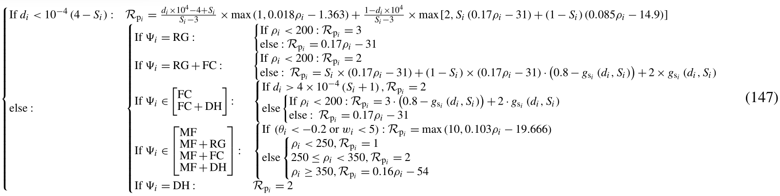

3.5.2 Shear strength

To be able to compute stability indexes of the snowpack, a shear resistance ${\mathcal{R}}_{{\mathrm{s}}_i}$ is diagnosed for each layer i. It is also computed from microstructure properties, density, liquid water content and temperature through Eq. (148). ${\mathcal{R}}_{{\mathrm{s}}_i}$ is expressed in kgf dm⁻² (1 kgf dm⁻² ≃ 0.981 kPa).

$$\begin{array}{}\text{(148)}& {\displaystyle }\left\{\begin{array}{ll}\left[\begin{array}{rl}{\displaystyle }\mathrm{If}& {\displaystyle }{w}_i\ge \mathrm{5}\\ {\displaystyle }\mathrm{and}& {\displaystyle }{\mathrm{\Psi }}_i\in \left\{\begin{array}{rl}{\displaystyle }& {\displaystyle }\mathrm{RG},\mathrm{MF},\mathrm{RG}+\mathrm{FC},\\ {\displaystyle }& {\displaystyle }\mathrm{RG}+\mathrm{MF},\mathrm{DF}+\mathrm{RG},\\ {\displaystyle }& {\displaystyle }\mathrm{MF}+\mathrm{FC},\mathrm{MF}+\mathrm{DH}\end{array}\right\}\end{array}\right]& \left\{\begin{array}{ll}\mathrm{If}{\mathit{\rho }}_i<\mathrm{200}:& {\mathcal{R}}_{{\mathrm{s}}_i}=\mathrm{0.1}\\ \mathrm{If}\mathrm{200}\le {\mathit{\rho }}_i<\mathrm{320}:& {\mathcal{R}}_{{\mathrm{s}}_i}=\mathrm{0.02}{\mathit{\rho }}_i-\mathrm{3.9}\\ \mathrm{If}{\mathit{\rho }}_i\ge \mathrm{320}:& {\mathcal{R}}_{{\mathrm{s}}_i}=\mathrm{0.068}{\mathit{\rho }}_i-\mathrm{18.64}\end{array}\right.\\ \mathrm{else}:& {\mathcal{R}}_{{\mathrm{s}}_i}=\max \left(\mathrm{0.05},{\mathcal{C}}_{\mathrm{1}}\left(S_i,h_i\right)\times {\mathcal{C}}_{\mathrm{2}}\left(d_i,S_i\right)\times {\mathcal{C}}_{\mathrm{3}}\left(d_i,S_i,h_i\right)\times {\mathcal{C}}_{\mathrm{4}}\left(w_i,{\mathit{\rho }}_i\right)\right.\\ & \left.\times {\mathcal{C}}_{\mathrm{5}}\left(d_i,S_i,h_i,w_i,{\mathit{\rho }}_i\right)\times \left({\mathit{\rho }}_i^{\mathrm{2}}\cdot {\mathrm{10}}^{-\mathrm{4}}-\mathrm{0.6}\right)+\mathrm{0.12}\right)\end{array}\right..\end{array}$$

𝒞₁, 𝒞₂, 𝒞₃, 𝒞₄ and 𝒞₅ multiplicative functions are defined in Appendix G.

3.6 MEPRA

MEPRA was a standalone module designed to estimate the avalanche hazard from the snowpack stratigraphy simulated by Crocus, from mechanical diagnosis and expert rules (Giraud et al., 2002). It has been fully implemented in the SURFEX platform, and its output are now available with the other diagnostic variables. The general idea is to compare the shear strength ${\mathcal{R}}_{{\mathrm{s}}_i}$ as defined previously, to the shear stress in the layer. For natural release, only the weight of overlying layers is taken into account while the load related to the presence of a skier at the snowpack surface is added to represent the accidental triggering. Expert rules are then defined to determine a hazard index from these mechanical stability indicators, both for natural release and accidental triggering. These expert rules were initially implemented by Giraud et al. (2002) but remained largely unpublished and have evolved to answer to feedbacks of operational avalanche forecasters, without detailed documentation. Equations implemented in the current version of SURFEX are described below. They are only valid for slope angle Θ=40°.

3.6.1 Mechanical stability of snowpack layers

A simple mechanical diagnosis for stability is computed by dividing the shear resistance ${\mathcal{R}}_{{\mathrm{s}}_i}$ by the shear in the layer. Two values are computed, to discriminate between natural avalanche activity and human triggering.

Natural release

The stability index ${\mathcal{S}}_{{\mathrm{nat}}_i}$ for natural release is defined in each layer i as follows:

$$\begin{array}{}\text{(149)}& {\mathcal{S}}_{{\mathrm{nat}}_i}={\displaystyle \frac{{\mathcal{R}}_{{\mathrm{s}}_i}}{{\mathit{\sigma }}_{i+\mathrm{1}}}}\end{array}$$

where σ_i+1 is the weight of overlying layers (including considered layers), projected on the slope-parallel axis, as defined by Eq. (52).

Accidental triggering

The stability index for accidental triggering ${\mathcal{S}}_{{\mathrm{acc}}_i}$ is similar to Eq. (149), with a supplementary term for shear stress to represent the additional load on the snowpack:

$$\begin{array}{}\text{(150)}& {\mathcal{S}}_{{\mathrm{acc}}_i}={\displaystyle \frac{{\mathcal{R}}_{{\mathrm{s}}_i}}{{\mathit{\sigma }}_{i+\mathrm{1}}+{\mathrm{\Xi }}_i{\mathit{\sigma }}_{{\mathrm{acc}}_i}}}\end{array}$$

where ${\mathit{\sigma }}_{{\mathrm{acc}}_i}$ is designed to represent the shear load induced by a skier, defined as a piecewise linear decreasing function of depth $Z_i=\sum _{j=\mathrm{1}}^i{z}_j$:

$$\begin{array}{}\text{(151)}& {\mathit{\sigma }}_{{\mathrm{acc}}_i}=\left\{\begin{array}{ll}\mathrm{4}-\mathrm{15}{Z}_i& \mathrm{if}{Z}_i<\mathrm{0.1}\\ \mathrm{2.5}-\mathrm{10}\left(Z_i-\mathrm{0.1}\right)& \mathrm{if}\mathrm{0.1}\le Z_i<\mathrm{0.15}\\ \mathrm{2}-\mathrm{8}\left(Z_i-\mathrm{0.15}\right)& \mathrm{if}\mathrm{0.15}\le Z_i<\mathrm{0.2}\\ \mathrm{1.6}-\mathrm{4}\left(Z_i-\mathrm{0.2}\right)& \mathrm{if}\mathrm{0.2}\le Z_i<\mathrm{0.35}\\ \mathrm{1}-\mathrm{2}\left(Z_i-\mathrm{0.35}\right)& \mathrm{if}\mathrm{0.35}\le Z_i<\mathrm{0.5}\\ \mathrm{0.7}-\mathrm{1.5}\left(Z_i-\mathrm{0.5}\right)& \mathrm{if}\mathrm{0.5}\le Z_i<\mathrm{0.8}\\ \mathrm{0}& \mathrm{if}\mathrm{0.8}\le Z_i\end{array}\right.\end{array}$$

and Ξ_i is designed to represent the bonding effect reducing the shear stress in the layers, defined by:

$$\begin{array}{}\text{(152)}& {\displaystyle }{\mathrm{\Xi }}_i={\displaystyle \frac{\sum _{j=\mathrm{1}}^i{m}_j{\mathit{\xi }}_j}{\sum j={\mathrm{1}}^i{m}_j}}\mathrm{where}{\mathit{\xi }}_i:\left\{\begin{array}{ll}\mathrm{If}{\mathrm{\Psi }}_i\in \left\{\begin{array}{rl}{\displaystyle }& {\displaystyle }\mathrm{MF},\mathrm{RG}+\mathrm{MF},\\ {\displaystyle }& {\displaystyle }\mathrm{MF}+\mathrm{FC},\mathrm{MF}+\mathrm{DF}\end{array}\right\}& \left\{\begin{array}{l}\mathrm{If}{\mathit{\theta }}_i<-\mathrm{0.2},{\mathit{\xi }}_i=\mathrm{0.5}\\ \mathrm{else}:{\mathit{\xi }}_i=\mathrm{1.1}\end{array}\right.\\ \text{else}:& \left\{\begin{array}{l}\mathrm{If}{\mathcal{R}}_{{\mathrm{s}}_i}>\mathrm{1.5}:{\mathit{\xi }}_i=\mathrm{1.0}\\ \mathrm{else}:{\mathit{\xi }}_i=\mathrm{1.2}\end{array}\right.\end{array}\right..\end{array}$$

3.6.2 Hazard indexes

MEPRA analyses the profiles of ${\mathcal{S}}_{{\mathrm{nat}}_i}$ and ${\mathcal{S}}_{{\mathrm{acc}}_i}$ mechanical indexes with other parameters (mainly grain type, temperature and liquid water content and snow heights), to assess a natural avalanche hazard index ℋ_nat, on a scale of 0–5 and accidental hazard index ℋ_acc on a scale 0–3, with a set of expert rules presented below. These hazard indexes are associated with levels of instability (one for high instability, Z_h, and one for moderate instability, Z_m, at most). For natural release, a classification between 5 avalanche types is also provided.

Natural release

The natural release analysis relies on a classification of the upper layers of the snowpack (referred as “superior profile”) in 4 classes: NEW (new snow), WET (wet snowpack), FRO (refrozen snowpack) or NAN (when it could not be classified in other class), based on the conditions listed in Table H1. A height of this superior profile Z_SUP is also defined below which the snowpack is significantly different, and called inferior profile. The latter is also classified into three classes : SOF (soft), HAR (hard) and NAN (undefined) as a function of the maximum penetration resistance, following Table H2.

Levels of high and moderate instabilities are looked for in the superior profile, as the uppermost buried layer where ${\mathcal{S}}_{{\mathrm{nat}}_i}$ is below a threshold 𝒮_h=2 or 𝒮_m=3 respectively (or 𝒮_m=3.05 for a NEW type of superior profile):

$$\begin{array}{}\text{(153)}& {\displaystyle }& {\displaystyle }\mathrm{If}\exists j|Z_j>\mathrm{0.1}\mathrm{and}{Z}_j\le Z_{\mathrm{SUP}}\mathrm{and}{\mathcal{S}}_{{\mathrm{nat}}_j}\le {\mathcal{S}}_{\mathrm{h}}:Z_{\mathrm{h}}=Z_j-{\displaystyle \frac{z_j}{\mathrm{2}}}\text{(154)}& {\displaystyle }& {\displaystyle }\mathrm{If}\exists k|Z_k>\mathrm{0.1}\mathrm{and}{Z}_j\le Z_{\mathrm{SUP}}\mathrm{and}{\mathcal{S}}_{{\mathrm{nat}}_j}\le {\mathcal{S}}_{\mathrm{m}}\mathrm{and}j\ne k:Z_{\mathrm{m}}=Z_k-{\displaystyle \frac{z_k}{\mathrm{2}}}.\end{array}$$

A first natural avalanche hazard index ℋ_nat is defined depending on depths of instability level Z_h and Z_m, superior profile height Z_SUP and superior profile type with the following expert rules:

$$\begin{array}{}\text{(155)}& {\displaystyle }\begin{array}{rlr}{\displaystyle }{\mathcal{H}}_{{\mathrm{nat}}_{\mathrm{1}}}=\left\{\begin{array}{l}{Z}_{\mathrm{h}}>\mathrm{0.8}\left\{\begin{array}{l}\mathrm{NEW}\to \mathrm{5}\\ \mathrm{WET}\to \mathrm{5}\\ \mathrm{FRO}\to \mathrm{3}\end{array}\right.\\ Z_{\mathrm{h}}>\mathrm{0.4}\left\{\begin{array}{l}\mathrm{NEW}\to \mathrm{4}\\ \mathrm{WET}\to \mathrm{4}\\ \mathrm{FRO}\to \mathrm{3}\end{array}\right.\\ Z_{\mathrm{h}}>\mathrm{0.2}\left\{\begin{array}{l}\mathrm{NEW}\to \mathrm{2}\\ \mathrm{WET}\to \mathrm{2}\\ \mathrm{FRO}\to \mathrm{3}\end{array}\right.\\ Z_{\mathrm{h}}>\mathrm{0}\left\{\begin{array}{l}\mathrm{NEW}\to \mathrm{1}\\ \mathrm{WET}\to \mathrm{1}\\ \mathrm{FRO}\to \mathrm{1}\end{array}\right.\\ Z_{\mathrm{h}}\mathrm{not}\mathrm{defined}\to \mathrm{0}\end{array}\right.& {\displaystyle }{\mathcal{H}}_{{\mathrm{nat}}_{\mathrm{2}}}=\left\{\begin{array}{l}{Z}_{\mathrm{m}}>\mathrm{0.8}\left\{\begin{array}{l}\mathrm{NEW}\to \mathrm{3}\\ \mathrm{WET}\to \mathrm{3}\\ \mathrm{FRO}\to \mathrm{1}\end{array}\right.\\ Z_{\mathrm{m}}>\mathrm{0.4}\left\{\begin{array}{l}\mathrm{NEW}\to \mathrm{3}\\ \mathrm{WET}\to \mathrm{3}\\ \mathrm{FRO}\to \mathrm{1}\end{array}\right.\\ Z_{\mathrm{m}}>\mathrm{0.2}\left\{\begin{array}{l}\mathrm{NEW}\to \mathrm{3}\\ \mathrm{WET}\to \mathrm{3}\\ \mathrm{FRO}\to \mathrm{1}\end{array}\right.\\ Z_{\mathrm{m}}>\mathrm{0}\left\{\begin{array}{l}\mathrm{NEW}\to \mathrm{1}\\ \mathrm{WET}\to \mathrm{1}\\ \mathrm{FRO}\to \mathrm{1}\end{array}\right.\\ Z_{\mathrm{m}}\mathrm{not}\mathrm{defined}\to \mathrm{0}\end{array}\right.& {\displaystyle }{\mathcal{H}}_{{\mathrm{nat}}_{\mathrm{3}}}=\left\{\begin{array}{l}{Z}_{\mathrm{SUP}}>\mathrm{0.8}\left\{\begin{array}{l}\mathrm{NEW}\to \mathrm{1}\\ \mathrm{WET}\to \mathrm{1}\\ \mathrm{FRO}\to \mathrm{0}\end{array}\right.\\ Z_{\mathrm{SUP}}>\mathrm{0.4}\left\{\begin{array}{l}\mathrm{NEW}\to \mathrm{1}\\ \mathrm{WET}\to \mathrm{1}\\ \mathrm{FRO}\to \mathrm{0}\end{array}\right.\\ Z_{\mathrm{SUP}}>\mathrm{0.2}\left\{\begin{array}{l}\mathrm{NEW}\to \mathrm{1}\\ \mathrm{WET}\to \mathrm{1}\\ \mathrm{FRO}\to \mathrm{0}\end{array}\right.\\ Z_{\mathrm{SUP}}>\mathrm{0}\left\{\begin{array}{l}\mathrm{NEW}\to \mathrm{0}\\ \mathrm{WET}\to \mathrm{1}\\ \mathrm{FRO}\to \mathrm{0}\end{array}\right.\\ Z_{\mathrm{SUP}}\mathrm{not}\mathrm{defined}\to \mathrm{0}\end{array}\right.\\ {\displaystyle }\mathrm{NEW},\mathrm{WET},\mathrm{or}\mathrm{FRO}& {\displaystyle }\to {\mathcal{H}}_{\mathrm{nat}}=\left\{\begin{array}{ll}\mathrm{2}& \mathrm{if}{\mathcal{H}}_{{\mathrm{nat}}_{\mathrm{1}}}=\mathrm{2}\\ \max \left({\mathcal{H}}_{{\mathrm{nat}}_{\mathrm{1}}},{\mathcal{H}}_{{\mathrm{nat}}_{\mathrm{2}}},{\mathcal{H}}_{{\mathrm{nat}}_{\mathrm{3}}}\right)& \mathrm{otherwise}\end{array}\right.\\ {\displaystyle }\mathrm{NAN}& {\displaystyle }\to {\mathcal{H}}_{\mathrm{nat}}=\mathrm{0}\end{array}.\end{array}$$

The avalanche situation is then classified in 6 classes following Appendix H2. Finally, ℋ_nat is updated by expert rules accounting from the temporal evolution between times t−Δt_M and t following Appendix H3. Note that these rules are sensitive to the MEPRA time step Δt_M, set to 3 h by Giraud et al. (2002).

Accidental triggering

ℋ_acc is based on the identification of a slab structure in the snowpack including a slab (layer i and possibly layers above) over a weak layer (layer i+1). This structure is identified through the following conditions:

$$\begin{array}{}\text{(156)}& \left\{\begin{array}{l}\mathrm{MF}\notin {\mathrm{\Psi }}_{i-\mathrm{1}}\\ {\mathcal{R}}_{{\mathrm{s}}_i}>\mathrm{1.3}\\ {\mathrm{\Psi }}_i\in [\mathrm{DF}+\mathrm{RG},\mathrm{RG},\mathrm{RG}+\mathrm{FC},\mathrm{DF}]\\ \mathrm{0.01}\mathrm{m}\le Z_i<\mathrm{1}\mathrm{m}\\ {\mathrm{\Psi }}_{i+\mathrm{1}}\in [\mathrm{FC},\mathrm{DH},\mathrm{FC}+\mathrm{DH},\mathrm{PP},\mathrm{PP}+\mathrm{DF},\mathrm{DF}]\end{array}\right..\end{array}$$

Similarly to the natural instability levels (Eqs. 153 and 154), levels of high accidental instability and moderate accidental instability are looked for among the identified weak layers satisfying Eq. (156):

$$\begin{array}{}\text{(157)}& {\displaystyle }& {\displaystyle }\mathrm{If}\exists i|{\mathrm{\Psi }}_{i+\mathrm{1}}\in [\mathrm{FC},\mathrm{DH},\mathrm{FC}+\mathrm{DH}]\mathrm{and}{\mathcal{S}}_{{\mathrm{acc}}_{i+\mathrm{1}}}<\mathrm{1.5}:Z_{\mathrm{h}}=Z_{i+\mathrm{1}}-{\displaystyle \frac{z_{i+\mathrm{1}}}{\mathrm{2}}}\text{(158)}& {\displaystyle }& {\displaystyle }\mathrm{If}\exists i|{\mathrm{\Psi }}_{i+\mathrm{1}}\in [\mathrm{PP},\mathrm{PP}+\mathrm{DF},\mathrm{DF}]\mathrm{or}\left({\mathrm{\Psi }}_{i+\mathrm{1}}\in [\mathrm{FC},\mathrm{DH},\mathrm{FC}+\mathrm{DH}]\mathrm{and}\mathrm{1.5}\le {\mathcal{S}}_{{\mathrm{acc}}_{i+\mathrm{1}}}<\mathrm{2.5}\right):Z_{\mathrm{m}}=Z_{i+\mathrm{1}}-{\displaystyle \frac{z_{i+\mathrm{1}}}{\mathrm{2}}}.\end{array}$$

The accidental hazard index is finally defined with the following expert rules:

$$\begin{array}{}\text{(159)}& \left\{\begin{array}{l}\mathrm{If}\exists i|\mathrm{Eq}.(\mathrm{159}):\left\{\begin{array}{l}\mathrm{If}{Z}_{\mathrm{c}}<\mathrm{0.01}:{\mathcal{H}}_{\mathrm{acc}}=\max \left(\mathrm{3},{\mathcal{H}}_{\mathrm{eq}}\right)\\ \mathrm{else}:{\mathcal{H}}_{\mathrm{acc}}=\max \left(\mathrm{1},{\mathcal{H}}_{\mathrm{eq}}\right)\end{array}\right.\\ \mathrm{If}\exists i|\mathrm{Eq}.(\mathrm{160}):\left\{\begin{array}{l}\mathrm{If}{Z}_{\mathrm{c}}<\mathrm{0.01}:{\mathcal{H}}_{\mathrm{acc}}=\max \left(\mathrm{2},{\mathcal{H}}_{\mathrm{eq}}\right)\\ \mathrm{else}:{\mathcal{H}}_{\mathrm{acc}}=\max \left(\mathrm{1},{\mathcal{H}}_{\mathrm{eq}}\right)\end{array}\right.\\ \mathrm{If}\textcolor{red}{}i|\mathrm{Eqs}.(\mathrm{159}\left)\mathrm{or}\right(\mathrm{160}):{\mathcal{H}}_{\mathrm{acc}}=\max \left(\mathrm{0},{\mathcal{H}}_{\mathrm{eq}}\right)\end{array}\right.\end{array}$$

where ℋ_eq  s a function of the natural index ℋ_nat following Appendix H4 and Z_c is the cumulated depth of crusts above a layer:

$$\begin{array}{}\text{(160)}& {\displaystyle }& {\displaystyle }{Z}_{{\mathrm{c}}_{\mathrm{h}}}=\sum _i{z}_i\mathrm{for}i|{\mathit{\theta }}_i<\mathrm{0.2}\mathrm{and}\mathrm{MF}\in {\mathrm{\Psi }}_i\mathrm{and}{Z}_i<Z_{\mathrm{h}}\mathrm{and}\left(\mathrm{PP}\notin {\mathrm{\Psi }}_j\mathrm{and}\mathrm{DF}\notin {\mathrm{\Psi }}_j\forall j\in [\mathrm{1},i-\mathrm{1}]\right)\text{(161)}& {\displaystyle }& {\displaystyle }{Z}_{{\mathrm{c}}_{\mathrm{m}}}=\sum _i{z}_i\mathrm{for}i|{\mathit{\theta }}_i<\mathrm{0.2}\mathrm{and}\mathrm{MF}\in {\mathrm{\Psi }}_i\mathrm{and}{Z}_i<Z_{\mathrm{m}}\mathrm{and}\left(\mathrm{PP}\notin {\mathrm{\Psi }}_j\mathrm{and}\mathrm{DF}\notin {\mathrm{\Psi }}_j\forall j\in [\mathrm{1},i-\mathrm{1}]\right.)\end{array}$$

Note that only one value for Z_h and Z_m is provided in the diagnoses output file. If ℋ_acc=ℋ_eq in Eq. (159), they correspond to Eqs. (153) and (154), otherwise they correspond to Eqs. (157) and (158).

4 Technical features

4.1 Implemented simulation geometries

All variables in the code are defined as vectors including at least a spatial dimension, and when necessary the snow layers as second dimension. The implication in terms of numerical efficiency of loops in the code is described in detail in Appendix J. This 1D spatial dimension allows to use either discontinuous collections of points or regular grids for simulations. A typical example of a collection of points is the semi-distributed geometry based on homogeneous massifs and topographic classes which has been used for more than 30 years for operational simulations in French mountains and in the associated 66-year reanalysis (Vernay et al., 2022). Gridded experiments can also be easily defined through the standard SURFEX tools which include regular latitude-longitude coordinates or various conformal projections. Over the French territory, the Lambert 93 projection is recommended as a national standard for gridded simulations (i.e. Deschamps-Berger et al., 2022; Haddjeri et al., 2024).

4.2 Parallelization and numerical efficiency

In the general case where Crocus is not coupled with a snow transport model, the processes currently represented by the model do not involve any mass or energy exchange between the snowpacks of the different spatial units. Therefore, parallelization can be very efficiently applied without any need of communication between processors in the physical model. A distributed memory parallelism has be chosen for that purpose in the offline driver of the SURFEX platform based on MPI libraries. However, the standard SURFEX Input-Output routines are not currently parallelized. Therefore, all input and output data are forwarded to a single processor. As a result, over large domains, the efficiency of parallel computing is currently limited by the saturation of the IO processor, in all cases but especially when the user chooses to output a large number of diagnoses at high temporal resolution. The XIOS library (Yepes-Arbós et al., 2022) implemented in SURFEX is designed to deal with this issue but the implementation of its compatibility with Crocus variables is still in progress. The numerical cost of the model itself depends on the number of layers created by the model. Therefore, it can vary significantly from one domain to another and from a season to another, depending on the number of layers of each simulated snowpack which highly depends on total snow depth.

To give the magnitude of the numerical cost, Table 3 presents the computing time of a 1-year simulation over 4471 simulation points in the French Alps. It must be noticed that the numerical cost of Crocus is very low compared to the cost of IO, providing a clear guidance for priorities in future optimizations. Crocus also only represents 26 % of the computation time of the ISBA land surface model itself. Even in an alpine region, the variability of snow cover in time and space makes the snow component relatively cheap with a similar level of complexity compared to the 20-layer soil model running all year over all points. As a result, the numerical cost of Crocus (0.3 cores × s per year and simulation point for this example) can not be considered as a valid argument to prefer simpler models in large scale applications of Land Surface Models or coupled applications.

Table 3 Numerical cost of a 1-year simulation from 1 August 023 to 1 August 2024 over 4471 simulation points corresponding to the French Alps domain described in Vernay et al. (2022) and the default physical options as in Lafaysse et al. (2017). The code was compiled with Intel®MPI library version 2018.5.274 and O₂ optimization level. Output are minimized (reduced to daily snow depth), otherwise the total execution time would be highly increased. The simulation is performed using 80 MPI threads on 80 physical cores on one 2.2 GHz AMD © Rome computing node constituted by 2 sockets of 64 cores. Results are presented in cores × s. The real elapsed time for this simulation in this architecture is 449 s.

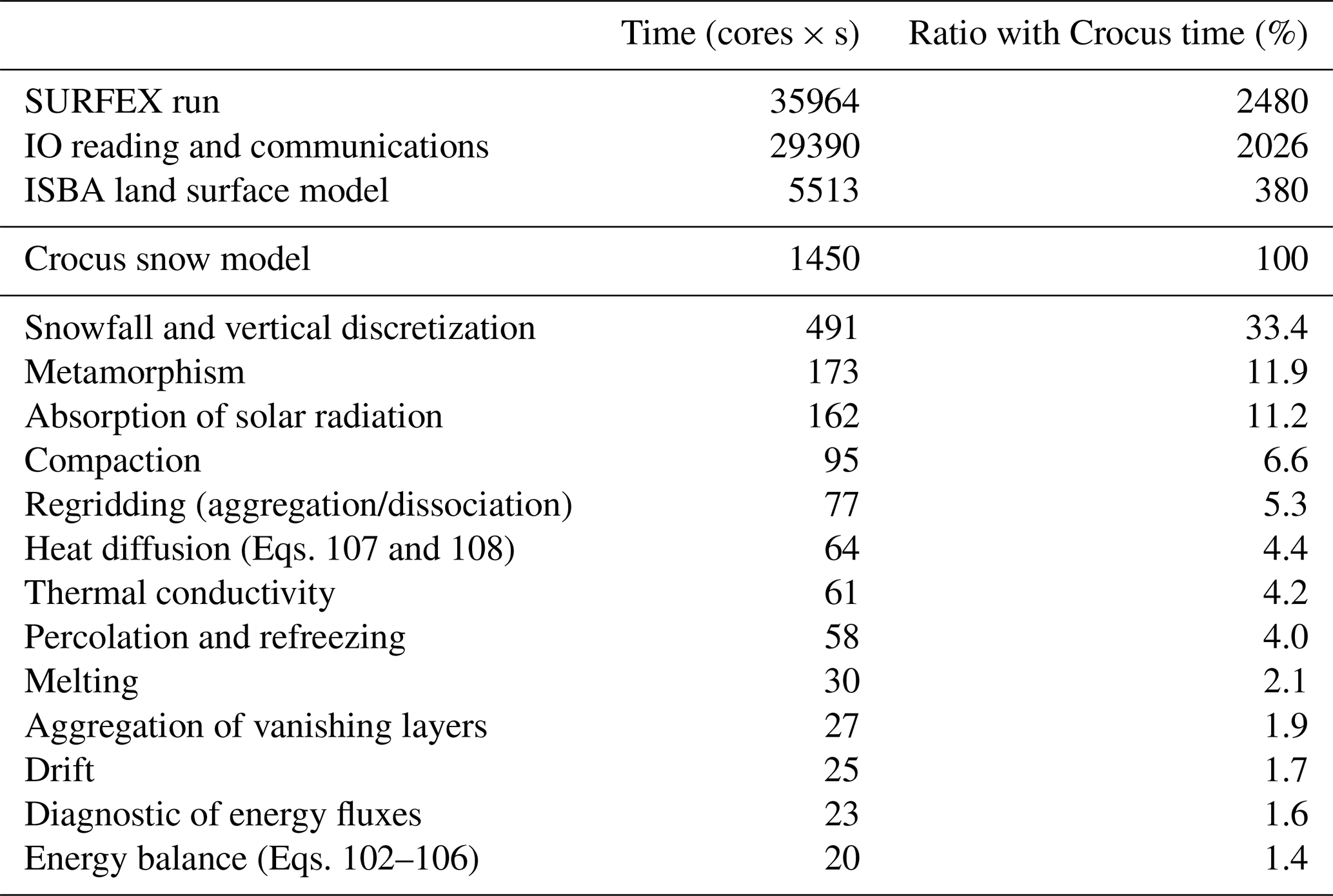
Considering the partitioning of numerical costs between the different subroutines within Crocus, it appears clearly that the complexity of the discretization rules emphasized by Eq. (11) has a significant impact as this routine represents 33 % of the whole model cost. The metamorphism routine is the second most contributing routine although its cost has been considerably reduced compared to previous versions (Carmagnola et al., 2014). The numerical core of the model solving heat diffusion and energy balance is very efficient contributing to less than 6 % of the cost. Numerical optimizations are still possible in some routines representing an unjustified contribution compared to their low complexity (e.g. thermal conductivity). Possible optimizations may concern the management of loops (cf. Appendix J) or some iterative calls to scalar functions in external modules.

The memory consumption of the model is relatively low with the standard physical options. In the experiment described above, the maximum Resident Set Size (RSS) is lower than 17 GB. However, the high spectral resolution of the TARTES optical scheme slightly increases the memory consumption (25 GB) and highly increases the total numerical cost when this option is activated (28 588 cores × s for the TARTES module in an experiment identical to Table 3 but with SNOWRAD = T17, i.e. about 20 times the reference numerical cost of Crocus).

4.3 Running environment and visualization

Beyond the FORTRAN code itself, most offline applications of the model have to deal with the management of input and output files to perform various experiments with different forcing files, namelists, or binaries, different setting of initial and final simulation dates, standard initialization procedures (soil spinup, etc.). Therefore, a common running environment of the model in Python is provided in an independent package called snowtools with full user documentation and an interface for technical support (cf. Code availability section).

Crocus scalar diagnoses can be easily processed by any scientific plotting software supporting netcdf format as input. However, the irregular vertical discretization of the snowpack model complexifies the visualization of the simulated profiles. A simple software provided in the snowtools package is able to combine the variables to plot with the depth of each layer to produce detailed instantaneous stratigraphies or temporal evolution of a given stratified variable (as in Appendix I). For spatial simulations, plotting the spatial variability of the vertical structure of the snowpack is still a challenge.

4.4 Externalization

Although the reference implementation of Crocus is within the SURFEX land surface modelling platform (Masson et al., 2013), there is an increasing need of being able to couple Crocus with other land surface schemes. For that purpose, an externalized version of the source codes is now available as an independent Fortran library that can be compiled alone and called by other land surface models (cf. Code availability section). It includes all the processes described in this paper except the coupling with external components (snow transport modules and MEB vegetation module). Thus, Crocus is also now fully integrated within the SVS2 land surface system (Vionnet et al., 2025). It was also recently implemented within the Flexible Snow Model (FSM2, Essery et al., 2025) allowing the coupling with its more detailed vegetation model (Mazzotti et al., 2024). SURFEX, SVS2 and FSM2 rely on a unique code repository of Crocus that guarantees the long-term maintenance and convergence of the code and therefore facilitates the contributions of different research groups to the model developments. For instance, as mentioned for several processes in Sect. 2, various new parameterizations better suited for Arctic snow were recently proposed within the SVS2 implementation (Woolley et al., 2024; Vionnet et al., 2025). Thanks to this method, these developments will integrate soon a future release and be beneficial for SURFEX and FSM2 applications. Therefore, we strongly encourage other groups that have copied the code within their specific applications to try to converge towards this unique code version. This includes the implementation of Crocus within WRF-Hydro (Eidhammer et al., 2021), the coupling of Crocus with Noah Land Surface Model (Navari et al., 2024), the MAR regional climate model largely used for polar regions (Fettweis et al., 2017; Agosta et al., 2019) and from which the Crocus version has diverged for a long time (Gallée et al., 2001), and even applications which have only extracted specific routines such as the CryoGrid permafrost model (Zweigel et al., 2021).

5 Review of evaluations and scientific applications

5.1 With a local scale meteorological forcing

The most direct evaluations of the model are performed on well-instrumented sites allowing to minimize errors in the meteorological forcing and in the observations used for evaluation. Model skills have been documented in detail at the Col de Porte experimental site (Morin et al., 2012; Lejeune et al., 2019), a mid-elevation meadow in French Alps. The very first evaluations of Brun et al. (1989) present qualitative evaluations of surface and internal temperature, snow depth, and basal runoff during short periods of the winter 1986–1987. Brun et al. (1992) extended the evaluations to the whole winter 1988–1989 on the same variables as well as a subjective comparison between the simulated stratigraphies and weekly observed profiles. Extensions of the evaluation period were successively published by Essery et al. (1999), Boone and Etchevers (2001), Strasser et al. (2002), Etchevers et al. (2004) and Avanzi et al. (2016) in the context of model intercomparisons, and also by Vionnet et al. (2012). These papers also included evaluations of albedo and Snow Water Equivalent. Lafaysse et al. (2017) extended these evaluations to all multiphysics options and accounted for observation uncertainties usually ignored in previous papers. The accuracy of the model on these variables has not significantly changed since the first years of development. Complementary evaluations of density and microstructure profiles are provided by Morin et al. (2013) and Carmagnola et al. (2014). However, quantitative evaluation of internal snow properties is still a methodological challenge due to frequent discrepancies between numerical and observed snow layers that can easily lead to double penalty issues. This can only be partly solved with vertical adjustments algorithms (Viallon-Galinier et al., 2020; Herla et al., 2021) or with an expert layer tracking (Calonne et al., 2020).

More challenging evaluations include a variety of environmental and climate conditions. Evaluations driven by local meteorological observations were performed in Svalbard (Bruland et al., 2001; Sauter and Obleitner, 2015), at the high elevation site of Weissflujoch, Switzerland (Etchevers et al., 2004), over tropical glaciers and moraines in Bolivia (Lejeune et al., 2007) and Ecuador (Wagnon et al., 2009), at Sherbrooke University, Quebec (Langlois. et al., 2009), at Torgnon, Italy (Di Mauro et al., 2019). The most comprehensive evaluations in terms of number of sites and years were performed on 10 contrasted sites through the Earth System Model-Snow Model Intercomparison Project (ESM-SnowMIP, Krinner et al., 2018; Menard et al., 2021) and with a few more sites for albedo evaluations by Gaillard et al. (2025). Typical errors on snow depth, SWE, albedo, surface temperature and ground temperature were in the range of state-of-the art snow models as illustrated with up-to-date simulations with this model version in Appendix I. A similar overall skill can be obtained by simpler models on these variables. The cold bias in surface temperature identified by Menard et al. (2021) may be attributed to the parameterization of turbulent fluxes which are suspected to be underestimated with the previously standard configuration (Ri_l=0.2) but this bias is removed with the new default value (Ri_l=0.026, Martin and Lejeune, 1998; Lafaysse et al., 2017). This assumption was also recently supported by more detailed evaluations of all components of the energy balance including eddy-covariance observations of turbulent fluxes in Québec (Lackner et al., 2022) and in Finnish peatlands (Nousu et al., 2024). However, it is especially important to be aware of the equifinality between the different empirical parameterizations (i.e. different model configurations providing similar model results) and to be cautious with the complex compromises in multivariate evaluations (the optimal model configuration can change depending on the evaluated variable, Essery et al., 2013; Lafaysse et al., 2017). These difficulties should encourage future attempts to improve processes representations to be tested robustly with ensemble multiphysics simulations and multivariate evaluations (e.g. Woolley et al., 2024).

5.2 With a regional scale meteorological forcing

In many other applications, the model was forced by meteorological reanalyses (e.g. Durand et al., 2009; Brun et al., 2013; Vernay et al., 2022) or short-term forecasts (e.g. Vionnet et al., 2016; Skaugen et al., 2018) or a combination of both (Vionnet et al., 2022). Although these studies often include snow depth evaluations on a large range of stations, in this case the resulting modelling errors of any snow model are dominated by errors in the meteorological forcing (Raleigh et al., 2015; Günther et al., 2019) and Crocus does not make an exception (Quéno et al., 2020; Réveillet et al., 2018; Vionnet et al., 2019; Gouttevin et al., 2022). Thus, the attribution of some limitations of the simulation results to the snowpack model itself is difficult. However, this is sometimes the only possible method for the assessment of some specific processes. For instance, the simulated concentrations of Light-Absorbing Particles (Tuzet et al., 2017), the spectral reflectances from the TARTES optical scheme (Cluzet et al., 2020), the blowing snow fluxes (Vionnet et al., 2018; Baron et al., 2024) were only evaluated in such context. The same applies to the ability of the model to reproduce the properties of polar snow (e.g. Dang et al., 1997; Libois et al., 2015; Barrere et al., 2017; Vionnet et al., 2025), the spatial distribution of snow conditions depending on topography (Revuelto et al., 2018; Skaugen et al., 2018; Haddjeri et al., 2024), or complex remote sensing signals (Veyssière et al., 2019). Similar simulation frameworks are used to investigate the suitability of the model for hydrological diagnoses (e.g. Strasser and Etchevers, 2005), glacier mass balance (e.g. Réveillet et al., 2018; Roussel et al., 2025) or avalanche activity (Eckert et al., 2010; Viallon-Galinier et al., 2022).

Based on the confidence provided by these available evaluations, the model is used for various purposes including the understanding of internal physical processes (e.g. Domine et al., 2013; Dick et al., 2023; Roussel et al., 2024), the quantification of contributions to the energy balance (e.g. Tuzet et al., 2020; Dumont et al., 2020; Réveillet et al., 2022, for light-absorbing particles), the monitoring of the long-term climatology of extreme snow loads (Le Roux et al., 2022) or avalanche activity (Reuter et al., 2022, 2025), the investigation of the links between snow cover and alpine ecosystems evolutions (Nicoud et al., 2025), and climate projections of natural snow conditions (Rousselot et al., 2012; Verfaillie et al., 2018), avalanche hazard (Castebrunet et al., 2014) and ski resorts operating conditions (Spandre et al., 2019; Morin et al., 2021; François et al., 2023). The development efforts were originally dedicated to operational avalanche hazard forecasting (Durand et al., 1999). However, after about 30 years of operation, the model did not become the main tool of the forecasters because this application is especially sensitive to uncertainties (Vernay et al., 2015) among numerous other challenges as reviewed by Morin et al. (2020). The statistical post-processing of simulations through various techniques of artifical intelligence (Nousu et al., 2019; Evin et al., 2021; Viallon-Galinier et al., 2023) might provide guidance to improve the practical interest of such simulations for operational applications including avalanche forecasting.

5.3 Towards data assimilation

The long memory of the snowpack on the past meteorological conditions and past snow processes imply that all sources of modelling errors tend to cumulate all along the season. Therefore, there is a large avenue for data assimilation algorithms in order to improve the initial states of the simulations (Largeron et al., 2020). However, the variable dimension size of the Crocus state vector (due to the variable number of layers) and the high non-linearities in the simulated processes make the application of a number of data assimilation algorithms to this model challenging. Therefore, most recent efforts intended to apply different variants of the Particle Filter to weight the members of an ensemble of simulations according to their distance to some observations (Charrois et al., 2016; Cluzet et al., 2021, 2022; Deschamps-Berger et al., 2022). The different options of the algorithm are described in Cluzet et al. (2021) and the implemented variables are snow depth and optical reflectance, for which the observation operator is simply the identity function as these variables are direct diagnoses of the model. The assimilation of optical reflectance is however constrained by the retrieval errors of this variable in complex terrain (Cluzet et al., 2020) that still exceed the requirements for an efficient data assimilation (Revuelto et al., 2021). Large efforts are planned in a near future to extend these possibilities. For some common satellite observations (e.g. snow cover fraction, wet snow fraction), this will require the development of appropriate observation operators from the simulated state variables.

6 Conclusion

This article provides a comprehensive description of all equations implemented in version 3.0.2 of the Crocus snow model. It gathers the recent developments of the last 13 years in a unique publication: (i) modelling of Light-Absorbing Particles, (ii) coupling with the TARTES optical scheme, (iii) modelling of ice layers due to freezing rain, (iv) coupling with the MEB big-leaf vegetation scheme, (v) snow management practices on ski slopes, (vi) coupling with blowing snow schemes, (vii) multiphysics parameterizations for most processes and (viii) diagnosis of the snowpack mechanical stability. In addition, this article documents a number of equations implemented in previous code versions but never published in the literature. It must be mentioned that during the preparation of this publication, a considerable number of errors or discrepancies between the code and previous publications were identified and corrected. This is in full agreement with the main conclusions of Menard et al. (2021) suggesting that insufficient model documentation is a key factor for the difficulty to improve snow modelling in the last decades. This comprehensive documentation is expected to help snow scientists to better interpret results based on this model. This is especially important in the context of an in-progress extension of Crocus applications in several land surface schemes. This documentation effort is also expected to help the snow modelling community improve numerical models in the future thanks to an accurate knowledge of the existing parameterizations and numerical difficulties. Despite our best efforts to minimize errors, previous literature and experience suggest that some errors may still remain in this publication. In such a case, corrigenda will be associated to this publication in due course.

Appendix A: Attractor profile in layering

The attractor profile $z_i^{*}$ used in Eq. (11) depends only on the total snow depth Z and number of layers N. Let us define N^* and Z^* by:

$$\begin{array}{}\text{(A1)}& \left\{\begin{array}{l}\mathrm{if}Z>\mathrm{20}\mathrm{and}N>\frac{N_{\max }}{\mathrm{3}}+\mathrm{2}\left\{\begin{array}{l}{N}^{*}=N-\frac{N+N_{\max }}{\mathrm{6}}\\ Z^{*}=\mathrm{3}\end{array}\right.\\ \mathrm{else}\left\{\begin{array}{l}{N}^{*}=N\\ Z^{*}=Z\end{array}\right.\end{array}\right..\end{array}$$

Then, the attractor profile is defined by:

$$\begin{array}{}\text{(A2)}& \left\{\begin{array}{l}{z}_{\mathrm{1}}^{*}=\min \left(\mathrm{0.01},\frac{Z^{*}}{N^{*}}\right)\\ z_{\mathrm{2}}^{*}=\min \left(\mathrm{0.0125},\frac{Z^{*}}{N^{*}}\right)\\ z_{\mathrm{3}}^{*}=\min \left(\mathrm{0.03},\frac{Z^{*}}{N^{*}}\right)\mathrm{if}{N}^{*}>\mathrm{3}\\ z_{\mathrm{4}}^{*}=\min \left(\mathrm{0.04},\frac{Z^{*}}{N^{*}}\right)\mathrm{if}{N}^{*}>\mathrm{4}\\ z_{\mathrm{5}}^{*}=\min \left(\mathrm{0.05},\frac{Z^{*}}{N^{*}}\right)\mathrm{if}{N}^{*}>\mathrm{5}\\ z_{\mathrm{6}}^{*}=\max \left(\mathrm{0.07},\min \left(\frac{Z^{*}}{N^{*}},\mathrm{0.5}\right)\right)\mathrm{if}{N}^{*}>\mathrm{6}\\ z_{\mathrm{7}}^{*}=\max \left(\mathrm{0.07},\min \left(\frac{Z^{*}}{N^{*}},\mathrm{1}.\right)\right)\mathrm{if}{N}^{*}>\mathrm{7}\\ z_{\mathrm{8}}^{*}=\max \left(\mathrm{0.07},\min \left(\frac{Z^{*}}{N^{*}},\mathrm{2}.\right)\right)\mathrm{if}{N}^{*}>\mathrm{8}\\ z_{\mathrm{9}}^{*}=\max \left(\mathrm{0.07},\min \left(\frac{Z^{*}}{N^{*}},\mathrm{4}.\right)\right)\mathrm{if}{N}^{*}>\mathrm{9}\\ z_{\mathrm{10}}^{*}=\max \left(\mathrm{0.07},\min \left(\frac{Z^{*}}{N^{*}},\mathrm{10}.\right)\right)\mathrm{if}{N}^{*}>\mathrm{10}\\ z_i^{*}=\max \left(\mathrm{0.07},\min \left(\frac{Z}{N},\right)\right)\forall i\in \left[\mathrm{11},N^{*}\right]\mathrm{if}{N}^{*}>\mathrm{11}\\ z_i^{*}=\left(i-N^{*}\right)\frac{\mathrm{2}(Z-\mathrm{3})}{\left(N-N^{*}\right)\left(N-N^{*}+\mathrm{1}\right)}\forall i\in \left[N^{*}+\mathrm{1},N\right]\mathrm{if}Z>\mathrm{20}\\ z_N^{*}=\min \left(\mathrm{0.02},\frac{Z}{N^{*}}\right)\\ \mathrm{if}Z>\mathrm{3}\mathrm{and}N*>\mathrm{10}\left\{\begin{array}{l}{z}_{N-\mathrm{1}}^{*}=\mathrm{0.66}{z}_N^{*}+\mathrm{0.34}{z}_{N-\mathrm{3}}^{*}\\ z_{N-\mathrm{2}}^{*}=\mathrm{0.34}{z}_N^{*}+\mathrm{0.66}{z}_{N-\mathrm{3}}^{*}\end{array}\right.\mathrm{instead}\mathrm{of}\mathrm{previous}\mathrm{definitions}\end{array}\right..\end{array}$$

It extends the definition of Vionnet et al. (2012) in order to converge towards a profile allowing a numerically stable resolution of heat diffusion for thick snowpacks and glacier applications.

Appendix B: Adjustment of wind speed

Several parameterizations of the model are formulated with a wind speed at a specific height corresponding to the experimental conditions but might not correspond to the reference height of the forcing variable. In these cases, the wind speed U_z (m s⁻¹) at height z (m) is adjusted assuming a logarithmic profile in the surface boundary layer based following:

$$\begin{array}{}\text{(B1)}& U_z=U{\displaystyle \frac{\ln \left(\frac{z}{z_{\mathrm{0}}}\right)}{\ln \left(\frac{z_u}{z_{\mathrm{0}}}\right)}}\end{array}$$

where z₀ is the surface roughness length (m).

Appendix C: Growth of faceted crystals in B21 metamorphism parameterizations

The growth of faceted crystals in B21 parameterization (Eq. 45) is based on cold room experiments from Marbouty (1980). These functions already published by Vionnet et al. (2012) are repeated here for the comprehensiveness of this paper. f, g, h and Φ are dimensionless functions from 0 to 1 given by:

$$\begin{array}{}\text{(C1)}& {\displaystyle }& {\displaystyle }f\left({\mathit{\theta }}_i\right)=\left\{\begin{array}{ll}\mathrm{0}& \mathrm{if}{\mathit{\theta }}_i<-\mathrm{40}\mathit{°}\mathrm{C}\\ \mathrm{0.011}\times \left({\mathit{\theta }}_i+\mathrm{40}\right)& \mathrm{if}-\mathrm{40}\le {\mathit{\theta }}_i<-\mathrm{22}\mathit{°}\mathrm{C}\\ \mathrm{0.2}+\mathrm{0.05}\times \left({\mathit{\theta }}_i+\mathrm{22}\right)& \mathrm{if}-\mathrm{22}\le {\mathit{\theta }}_i<-\mathrm{6}\mathit{°}\mathrm{C}\\ \mathrm{0.7}-\mathrm{0.05}{\mathit{\theta }}_i& \mathrm{otherwise}\end{array}\right.\text{(C2)}& {\displaystyle }& {\displaystyle }h\left({\mathit{\rho }}_i\right)=\left\{\begin{array}{ll}\mathrm{1}.& \mathrm{if}{\mathit{\rho }}_i<\mathrm{150}\mathrm{kg}{\mathrm{m}}^{-\mathrm{3}}\\ \mathrm{1}-\mathrm{0.004}\times \left({\mathit{\rho }}_i-\mathrm{150}\right)& \mathrm{if}\mathrm{150}<{\mathit{\rho }}_i<\mathrm{400}\mathrm{kg}{\mathrm{m}}^{-\mathrm{3}}\\ \mathrm{0}.& \mathrm{otherwise}\end{array}\right.\text{(C3)}& {\displaystyle }& {\displaystyle }g\left({\mathcal{G}}_i\right)=\left\{\begin{array}{ll}\mathrm{0}.& \mathrm{if}{\mathcal{G}}_i<\mathrm{15}\mathrm{K}{\mathrm{m}}^{-\mathrm{1}}\\ \mathrm{0.01}\times \left({\mathcal{G}}_i-\mathrm{15}\right)& \mathrm{if}\mathrm{15}\le {\mathcal{G}}_i<\mathrm{25}\mathrm{K}{\mathrm{m}}^{-\mathrm{1}}\\ \mathrm{0.1}+\mathrm{0.037}\times \left({\mathcal{G}}_i-\mathrm{25}\right)& \mathrm{if}\mathrm{25}\le {\mathcal{G}}_i<\mathrm{40}\mathrm{K}{\mathrm{m}}^{-\mathrm{1}}\\ \mathrm{0.65}+\mathrm{0.02}\times \left({\mathcal{G}}_i-\mathrm{40}\right)& \mathrm{if}\mathrm{40}\le {\mathcal{G}}_i<\mathrm{50}\mathrm{K}{\mathrm{m}}^{-\mathrm{1}}\\ \mathrm{0.85}+\mathrm{0.0075}\times \left({\mathcal{G}}_i-\mathrm{50}\right)& \mathrm{if}\mathrm{50}\le {\mathcal{G}}_i<\mathrm{70}\mathrm{K}{\mathrm{m}}^{-\mathrm{1}}\\ \mathrm{1}.& \mathrm{otherwise}\end{array}\right.\text{(C4)}& {\displaystyle }& {\displaystyle }\mathrm{\Phi }={\mathrm{1.0417.10}}^{-\mathrm{9}}\mathrm{m}{\mathrm{s}}^{-\mathrm{1}}.\end{array}$$

Appendix D: New formalism of metamorphism

The translation of the original metamorphism parameterizations in terms of dendricity, sphericity and size from Brun et al. (1992) to the new formalism of Carmagnola et al. (2014) in terms of optical diameter and sphericity, was based on the original expression of the optical diameter d_i as a function of dendricity δ_i, sphericity S_i and grain size $g_{s_i}$ (as already published in Eq. 13 of Vionnet et al., 2012):

$$\begin{array}{}\text{(D1)}& d_i=\left\{\begin{array}{ll}{\mathrm{10}}^{-\mathrm{4}}\left[{\mathit{\delta }}_i+\left(\mathrm{1}-{\mathit{\delta }}_i\right)\left(\mathrm{4}-S_i\right)\right]& \mathrm{if}{\mathit{\delta }}_i>\mathrm{0}\left(\mathrm{dendritic}\mathrm{case}\right)\\ g_{s_i}\times S_i+\left(\mathrm{1}-S_i\right)\times \max \left({\mathrm{4.10}}^{-\mathrm{4}},\frac{g_{s_i}}{\mathrm{2}}\right)& \mathrm{if}{\mathit{\delta }}_i=\mathrm{0}\left(\mathrm{non}\text{-}\mathrm{dendritic}\mathrm{case}\right)\end{array}\right..\end{array}$$

This relationship has always been required to compute the absorption of solar radiation from the equations of Sect. 2.4.9.

In the dendritic case, the transformation $(S_i,{\mathit{\delta }}_i)\Rightarrow (S_i,d_i)$ is bijective. The inversion of this relationship lead to:

$$\begin{array}{}\text{(D2)}& {\mathit{\delta }}_i={\displaystyle \frac{{\mathrm{10}}^{\mathrm{4}}\times d_i-\mathrm{4}+S_i}{S_i-\mathrm{3}}}\mathrm{if}{d}_i<{\mathrm{10}}^{-\mathrm{4}}\left(\mathrm{4}-S_i\right)\end{array}$$

and the new evolution law of d_i was obtained by Carmagnola et al. (2014) using

$$\begin{array}{}\text{(D3)}& {\displaystyle \frac{\mathrm{d}{d}_i}{\mathrm{d}t}}={\displaystyle \frac{\partial d_i}{\partial {\mathit{\delta }}_i}}{\displaystyle \frac{\mathrm{d}{\mathit{\delta }}_i}{\mathrm{d}t}}+{\displaystyle \frac{\partial d_i}{\partial S_i}}{\displaystyle \frac{\mathrm{d}{S}_i}{\mathrm{d}t}}.\end{array}$$

Thus, the combination of Eq. (D3) with the equations from Table 1 of Vionnet et al. (2012) provides the second line of Eq. (45) in this paper (which is close to the right column of Table 2 in Carmagnola et al., 2014 after typo corrections).

In the non-dendritic case, the transformation $(S_i,g_{s_i})\Rightarrow (S_i,d_i)$ is not bijective. When S_i=0, Eq. (D1) gives $d_i=\mathrm{4}\times {\mathrm{10}}^{-\mathrm{4}}\forall g_{s_i}\in [\mathrm{3}\times {\mathrm{10}}^{-\mathrm{4}},\mathrm{8}\times {\mathrm{10}}^{-\mathrm{4}}]$. As a result, the metamorphism functions from Table 1 of Vionnet et al. (2012) cannot be reproduced in the space (S_i, d_i) when S_i=0 (e.g. depth hoar). Then, Eq. (D1) is discontinuous at the limit between dendritic and non-dendritic cases. Indeed, the limit of the dendritic case gives $\underset{{\mathit{\delta }}_i\to \mathrm{0}}{lim}{d}_i={\mathrm{10}}^{-\mathrm{4}}(\mathrm{4}-S_i)$. When combined with the non dendritic case, this would result in $g_{s_i}=\mathrm{3}\times {\mathrm{10}}^{-\mathrm{4}}$ while the initial value of $g_{s_i}$ was actually higher for non-spheric particles in Brun et al. (1992): $g_{s_i}={\mathrm{10}}^{-\mathrm{4}}(\mathrm{4}-s_i)$. In the other cases, the inversion of Eq. (D1) can provide a relationship for $g_{s_i}$ as a function of d_i and S_i:

$$\begin{array}{}\text{(D4)}& g_{s_i}=\left\{\begin{array}{ll}\mathrm{2}\frac{d_i}{S_i+\mathrm{1}}& \mathrm{if}{d}_i\ge \mathrm{4}\times {\mathrm{10}}^{-\mathrm{4}}\left(S_i+\mathrm{1}\right)\\ \frac{d_i-\mathrm{4}\times {\mathrm{10}}^{-\mathrm{4}}\left(\mathrm{1}-S_i\right)}{S_i}& \mathrm{if}{d}_i<\mathrm{4}\times {\mathrm{10}}^{-\mathrm{4}}\left(S_i+\mathrm{1}\right)\end{array}\right..\end{array}$$

Equation (D4) is actually more complex than Eq. (3) of Carmagnola et al. (2014) which was an incorrect simplification corresponding only to the initialization of grain size at the dendritic - non-dendritic transition. It is also not defined when S_i=0 and $d_i<\mathrm{4}\times {\mathrm{10}}^{-\mathrm{4}}(S_i+\mathrm{1})$. Last, the derivation of an evolution law for optical diameter was obtained by Carmagnola et al. (2014) in the non-dendritic case (left column of their Table 2) by considering only $\frac{\mathrm{d}{d}_i}{\mathrm{d}t}=\frac{\partial d_i}{\partial S_i}\frac{\mathrm{d}{S}_i}{\mathrm{d}t}$. This is actually inconsistent with the original formalism in the non-dendritic case as it ignores the term $\frac{\partial d_i}{\partial g_{s_i}}\frac{\mathrm{d}{g}_{s_i}}{\mathrm{d}t}$. Ignoring this term may be convenient to avoid the problems mentioned above but it affects the metamorphism of faceted crystals and depth hoar without any scientific justification whereas they are the most critical snow types for further analyses in terms of mechanical stability. Furthermore, a number of parameterizations of other processes and diagnoses in the code were also affected by the incorrect simplification of Eq. (D4). The original difficulty of this translation of formalisms comes from the fact that Eq. (D1) is neither bijective nor continuous. However, we considered that it is better to adapt this unpublished formula and preserve as much as possible the metamorphism laws, the parameterizations of other processes and the diagnoses relying on microstructure properties. A new metamorphism option (B21) has therefore been defined, replacing the expression from Carmagnola et al. (2014) by:

$$\begin{array}{}\text{(D5)}& d_i=g_{s_i}\times S_i+\left(\mathrm{1}-S_i\right){\displaystyle \frac{\mathrm{4}\times {\mathrm{10}}^{-\mathrm{4}}+g_{s_i}}{\mathrm{2}}}\mathrm{if}{\mathit{\delta }}_i=\mathrm{0}\left(\mathrm{non}\text{-}\mathrm{dendritic}\mathrm{case}\right).\end{array}$$

This allows to replace Eq. (D4) by:

$$\begin{array}{}\text{(D6)}& g_{s_i}=\mathrm{2}{\displaystyle \frac{d_i-\mathrm{2}\times {\mathrm{10}}^{-\mathrm{4}}\left(\mathrm{1}-S_i\right)}{\mathrm{1}+S_i}}.\end{array}$$

This way, the evolution of optical diameter in the non dendritic case can be obtained by:

$$\begin{array}{}\text{(D7)}& {\displaystyle \frac{\mathrm{d}{d}_i}{\mathrm{d}t}}& {\displaystyle }={\displaystyle \frac{\partial d_i}{\partial g_{s_i}}}{\displaystyle \frac{\mathrm{d}{g}_{s_i}}{\mathrm{d}t}}+{\displaystyle \frac{\partial d_i}{\partial S_i}}{\displaystyle \frac{\mathrm{d}{S}_i}{\mathrm{d}t}}\text{(D8)}& {\displaystyle }& {\displaystyle }={\displaystyle \frac{\mathrm{1}+S_i}{\mathrm{2}}}{\displaystyle \frac{\mathrm{d}{g}_{s_i}}{\mathrm{d}t}}+\left({\displaystyle \frac{g_{s_i}}{\mathrm{2}}}-\mathrm{2}\times {\mathrm{10}}^{-\mathrm{4}}\right){\displaystyle \frac{\mathrm{d}{S}_i}{\mathrm{d}t}}\text{(D9)}& {\displaystyle }& {\displaystyle }={\displaystyle \frac{\mathrm{1}+S_i}{\mathrm{2}}}{\displaystyle \frac{\mathrm{d}{g}_{s_i}}{\mathrm{d}t}}+{\displaystyle \frac{d_i-\mathrm{4}\times {\mathrm{10}}^{-\mathrm{4}}}{\mathrm{1}+S_i}}{\displaystyle \frac{\mathrm{d}{S}_i}{\mathrm{d}t}}.\end{array}$$

The main advantage of this new formalism is that it respects the original evolution law of $\frac{\mathrm{d}{g}_{s_i}}{\mathrm{d}t}$ as published by Vionnet et al. (2012). As a result, all parameterizations and diagnostics calibrated in the original formalism can still considered to be valid in this new formalism. Finally, the first line of Eq. (45) corresponds to the combination of Eq. (D9) and Table 1 of Vionnet et al. (2012). Complementary analyses by Baron (2023) have shown that the obtained microstructure properties of B21 option are closer to the original formalism of Vionnet et al. (2012) than the implementation of Carmagnola et al. (2014) (also referred as C13 in Lafaysse et al. (2017). This is especially true when this parameterization is combined with the snow drift options. More details are available in Baron (2023).

Similarly for wet metamorphism, the combination of Eq. (D9) and Table   of Vionnet et al. (2012) provides Eq. (49) of this paper. The transformation of wet metamorphism laws in this new formalism were neither provided in Carmagnola et al. (2014) nor correctly implemented.

Appendix E: Evolution of optical diameter during snow drift

The evolution of microstructure properties was parameterized in terms of dendricity δ_i, sphericity S_i and grain size $g_{s_i}$ from simple evolution laws provided in Table 3 of Vionnet et al. (2012) in which sign errors must be accounted for in the evolution of δ_i and $g_{s_i}$:

$$\begin{array}{}\text{(E1)}& {\displaystyle }& {\displaystyle \frac{\mathrm{d}{\mathit{\delta }}_i}{\mathrm{d}t}}={\displaystyle \frac{-{\mathit{\delta }}_i}{\mathrm{2}{\mathit{\tau }}_{\mathrm{DRIFT}}}}\mathrm{if}{\mathit{\delta }}_i>\mathrm{0}\left(\mathrm{dendritic}\mathrm{case}\right)\text{(E2)}& {\displaystyle }& {\displaystyle \frac{\mathrm{d}{g}_{s_i}}{\mathrm{d}t}}={\displaystyle \frac{-\mathrm{5}\times {\mathrm{10}}^{-\mathrm{4}}}{{\mathit{\tau }}_{\mathrm{DRIFT}}}}\mathrm{if}{\mathit{\delta }}_i=\mathrm{0}\left(\mathrm{non}\text{-}\mathrm{dendritic}\mathrm{case}\right)\text{(E3)}& {\displaystyle }& {\displaystyle \frac{\mathrm{d}{S}_i}{\mathrm{d}t}}={\displaystyle \frac{\mathrm{1}-S_i}{{\mathit{\tau }}_{\mathrm{DRIFT}}}}.\end{array}$$

In the dendritic case, the evolution of the optical diameter d_i is obtained by the introduction of Eqs. (E1) and (E3) in Eq. (D3) and computing $\frac{\partial di}{\partial {\mathit{\delta }}_i}$ and $\frac{\partial d_i}{\partial S_i}$ from the first line of Eq. (D1). In the non-dendritic case, the evolution of the optical diameter d_i is obtained by the introduction of Eqs. (E2) and (E3) in Eq. (D7) and computing $\frac{\partial d_i}{\partial g_{s_i}}$ and $\frac{\partial d_i}{\partial S_i}$ from Eq. (D5). Finally:

$$\begin{array}{}\text{(E4)}& \left\{\begin{array}{rlr}{\displaystyle \frac{\mathrm{d}{d}_i}{\mathrm{d}t}}& {\displaystyle }={\mathrm{10}}^{-\mathrm{4}}\left(S_i-\mathrm{3}\right)\times \left({\displaystyle \frac{-{\mathit{\delta }}_i}{\mathrm{2}{\mathit{\tau }}_{\mathrm{DRIFT}}}}\right)+{\mathrm{10}}^{-\mathrm{4}}\left({\mathit{\delta }}_i-\mathrm{1}\right)\times {\displaystyle \frac{\mathrm{1}-S_i}{{\mathit{\tau }}_{\mathrm{DRIFT}}}}& {\displaystyle }\mathrm{if}{d}_i<{\mathrm{10}}^{-\mathrm{4}}\left(\mathrm{4}-S_i\right)\\ {\displaystyle \frac{\mathrm{d}{d}_i}{\mathrm{d}t}}& {\displaystyle }={\displaystyle \frac{S_i+\mathrm{1}}{\mathrm{2}}}\times {\displaystyle \frac{-\mathrm{5}\times {\mathrm{10}}^{-\mathrm{4}}}{{\mathit{\tau }}_{\mathrm{DRIFT}}}}+{\displaystyle \frac{g_{s_i}-\mathrm{4}\times {\mathrm{10}}^{-\mathrm{4}}}{\mathrm{2}}}\times {\displaystyle \frac{\mathrm{1}-S_i}{{\mathit{\tau }}_{\mathrm{DRIFT}}}}& {\displaystyle }\mathrm{if}{d}_i\ge {\mathrm{10}}^{-\mathrm{4}}\left(\mathrm{4}-S_i\right).\end{array}\right.\end{array}$$

The first line can be slightly simplified and Eq. (D6) introduced in the second line to finally obtain the equivalent discrete formulation of Eq. (65).

Appendix F: Thermodynamical functions

The air volumetric mass ρ_a is obtained by:

$$\begin{array}{}\text{(F1)}& {\mathit{\rho }}_{\mathrm{a}}={\displaystyle \frac{P_{\mathrm{s}}}{R_{\mathrm{a}}{T}_{\mathrm{a}}\left(\mathrm{1}+\left(\frac{R_{\mathrm{v}}}{R_{\mathrm{a}}}-\mathrm{1}\right)q_{\mathrm{a}}\right)+g\times z_{\mathrm{a}}}}.\end{array}$$

The Exner functions at surface and at the forcing level are defined by:

$$\begin{array}{}\text{(F2)}& {\displaystyle }& {\displaystyle }{\mathrm{\Pi }}_{\mathrm{a}}={\left({\displaystyle \frac{P_{\mathrm{a}}}{P_{\mathrm{0}}}}\right)}^{\frac{R_{\mathrm{a}}}{c_{\mathrm{P}}}}\text{(F3)}& {\displaystyle }& {\displaystyle }{\mathrm{\Pi }}_{\mathrm{s}}={\left({\displaystyle \frac{P_{\mathrm{s}}}{P_{\mathrm{0}}}}\right)}^{\frac{R_{\mathrm{a}}}{c_{\mathrm{P}}}}\end{array}$$

where P₀=10⁵ Pa and the atmospheric pressure at forcing level P_a is obtained from hydrostatism:

$$\begin{array}{}\text{(F4)}& P_{\mathrm{a}}=P_{\mathrm{s}}-{\mathit{\rho }}_{\mathrm{a}}g{z}_{\mathrm{a}}.\end{array}$$

The saturation specific humidity at temperature T is obtained by:

$$\begin{array}{}\text{(F5)}& q_{\mathrm{sat}}\left(T,P_{\mathrm{s}}\right)={\displaystyle \frac{\frac{R_{\mathrm{a}}}{R_{\mathrm{v}}}\times \frac{e_{\mathrm{sat}}\left(T\right)}{P_{\mathrm{s}}}}{\mathrm{1}+\left(\frac{R_{\mathrm{a}}}{R_{\mathrm{v}}}-\mathrm{1}\right)\frac{e_{\mathrm{sat}}\left(T\right)}{P_{\mathrm{s}}}}}\end{array}$$

where the water vapor partial pressure at saturation e_sat(T) is obtained from Eq. (F6) which is an approximate integral of the Clausius–Clapeyron formula:

$$\begin{array}{}\text{(F6)}& \left\{\begin{array}{l}\mathrm{If}T\ge T_{\mathrm{0}}{e}_{\mathrm{sat}}\left(T\right)=\exp \left({\mathit{\alpha }}_{\mathrm{w}}-\frac{{\mathit{\beta }}_{\mathrm{w}}}{T}-{\mathit{\gamma }}_{\mathrm{w}}\ln \left(T\right)\right)\\ \mathrm{If}T<T_{\mathrm{0}}{e}_{\mathrm{sat}}\left(T\right)=\exp \left({\mathit{\alpha }}_{\mathrm{I}}-\frac{{\mathit{\beta }}_{\mathrm{I}}}{T}-{\mathit{\gamma }}_{\mathrm{I}}\ln \left(T\right)\right)\end{array}\right.\end{array}$$

where

$$\begin{array}{}\text{(F7)}& {\displaystyle }& {\displaystyle }{\mathit{\gamma }}_{\mathrm{w}}={\displaystyle \frac{c_{\mathrm{W}}-c_{{\mathrm{P}}_{\mathrm{v}}}}{R_{\mathrm{v}}}}\text{(F8)}& {\displaystyle }& {\displaystyle }{\mathit{\beta }}_{\mathrm{w}}={\displaystyle \frac{L_{\mathrm{v}}}{R_{\mathrm{v}}}}+{\mathit{\gamma }}_{\mathrm{w}}{T}_{\mathrm{0}}\text{(F9)}& {\displaystyle }& {\displaystyle }{\mathit{\alpha }}_{\mathrm{w}}=\ln \left(e_{\mathrm{sat}}\left(T_{\mathrm{0}}\right)\right)+{\displaystyle \frac{{\mathit{\beta }}_{\mathrm{w}}}{T_{\mathrm{0}}}}+{\mathit{\gamma }}_{\mathrm{w}}\ln \left(T_{\mathrm{0}}\right)\text{(F10)}& {\displaystyle }& {\displaystyle }{\mathit{\gamma }}_{\mathrm{I}}={\displaystyle \frac{c_{\mathrm{I}}-c_{{\mathrm{P}}_{\mathrm{v}}}}{R_{\mathrm{v}}}}\text{(F11)}& {\displaystyle }& {\displaystyle }{\mathit{\beta }}_{\mathrm{I}}={\displaystyle \frac{L_{\mathrm{s}}}{R_{\mathrm{v}}}}+{\mathit{\gamma }}_{\mathrm{I}}{T}_{\mathrm{0}}\text{(F12)}& {\displaystyle }& {\displaystyle }{\mathit{\alpha }}_{\mathrm{I}}=\ln \left(e_{\mathrm{sat}}\left(T_{\mathrm{0}}\right)\right)+{\displaystyle \frac{{\mathit{\beta }}_{\mathrm{I}}}{T_{\mathrm{0}}}}+{\mathit{\gamma }}_{\mathrm{I}}\ln \left(T_{\mathrm{0}}\right)\text{(F13)}& {\displaystyle }& {\displaystyle }{e}_{\mathrm{sat}}\left(T_{\mathrm{0}}\right)=\mathrm{611.14}\mathrm{Pa}.\end{array}$$

The derivative $\frac{\partial q_{\mathrm{sat}}(T,P_{\mathrm{s}})}{\partial T}$ is obtained by:

$$\begin{array}{}\text{(F14)}& {\displaystyle \frac{\partial q_{\mathrm{sat}}\left(T,P_{\mathrm{s}}\right)}{\partial T}}={\displaystyle \frac{\partial e_{\mathrm{sat}}\left(T\right)}{\partial T}}{q}_{\mathrm{sat}}\left(T,P_{\mathrm{s}}\right)\times {\displaystyle \frac{\mathrm{1}}{\mathrm{1}+\frac{\frac{R_{\mathrm{a}}}{R_{\mathrm{v}}}-\mathrm{1}}{\mathrm{1}+\frac{R_{\mathrm{a}}}{R_{\mathrm{v}}}\left(\frac{\mathrm{1}}{q_{\mathrm{sat}}\left(T,P_{\mathrm{s}}\right)}-\mathrm{1}\right)}}}\end{array}$$

where

$$\begin{array}{}\text{(F15)}& {\displaystyle \frac{\partial e_{\mathrm{sat}}\left(T\right)}{\partial T}}={\displaystyle \frac{{\mathit{\beta }}_{\mathrm{w}}}{T^{\mathrm{2}}}}-{\displaystyle \frac{{\mathit{\gamma }}_{\mathrm{w}}}{T}}.\end{array}$$

The Richardson number is computed by:

$$\begin{array}{}\text{(F16)}& Ri=g\cos \mathrm{\Theta }{z}_u^{\mathrm{2}}{\displaystyle \frac{{\mathit{\theta }}_{v_{\mathrm{a}}}-{\mathit{\theta }}_{v_{\mathrm{s}}}}{\mathrm{0.5}\left({\mathit{\theta }}_{v_{\mathrm{a}}}+{\mathit{\theta }}_{v_{\mathrm{s}}}\right)\max {\left(U,U_{\mathrm{th}}\right)}^{\mathrm{2}}{z}_{\mathrm{a}}}}\end{array}$$

where

$$\begin{array}{}\text{(F17)}& {\displaystyle }& {\displaystyle }{\mathit{\theta }}_{v_{\mathrm{a}}}={\displaystyle \frac{T_{\mathrm{a}}}{{\mathrm{\Pi }}_{\mathrm{a}}}}\left(\mathrm{1}+\left({\displaystyle \frac{R_{\mathrm{v}}}{R_{\mathrm{a}}}}-\mathrm{1}\right)q_{\mathrm{a}}\right)\text{(F18)}& {\displaystyle }& {\displaystyle }{\mathit{\theta }}_{v_{\mathrm{s}}}={\displaystyle \frac{T_{\mathrm{1}}}{{\mathrm{\Pi }}_{\mathrm{s}}}}\left(\mathrm{1}+\left({\displaystyle \frac{R_{\mathrm{v}}}{R_{\mathrm{a}}}}-\mathrm{1}\right)q_{\mathrm{sat}}\left(T_{\mathrm{1}},P_{\mathrm{s}}\right)\right).\end{array}$$

The wet bulb temperature $T_{\mathrm{w}}^{*}$ (°C) is computed by Eq. (F19):

$$\begin{array}{}\text{(F19)}& T_{\mathrm{w}}^{*}={\displaystyle \frac{\mathit{\gamma }\cdot T_{\mathrm{a}}^{*}+\frac{\partial e_{\mathrm{sat}}\left(T\right)}{\partial T}\cdot T_{\mathrm{d}}^{*}}{\mathit{\gamma }+\frac{\partial e_{\mathrm{sat}}\left(T\right)}{\partial T}}}\end{array}$$

where the slope of the saturation vapor pressure curve $\frac{\partial e_{\mathrm{sat}}\left(T\right)}{\partial T}$ is given by Eq. (F15); the dew point temperature $T_{\mathrm{d}}^{*}$ (°C) is parameterized by

$$\begin{array}{}\text{(F20)}& T_{\mathrm{d}}^{*}=[\mathrm{116.9}+\mathrm{237.3}\ln (e\left)\right]/[\mathrm{16.78}-\ln (e\left)\right].\end{array}$$

and the psychrometric constant γ (in kPa K⁻¹) is obtained by:

$$\begin{array}{}\text{(F21)}& \mathit{\gamma }={\displaystyle \frac{c_{P_{\mathrm{m}}}\cdot P_{\mathrm{s}}}{\mathrm{0.622}\cdot L_{\mathrm{v}}}}\end{array}$$

where $c_{P_{\mathrm{m}}}$ is the specific heat capacity of moist air at constant pressure (in kJ kg⁻¹ °C⁻¹).

Appendix G: Functions in the parameterization of shear resistance

$$\begin{array}{}\text{(G1)}& {\displaystyle }\left\{\begin{array}{ll}\mathrm{If}{S}_i>\mathrm{0.8}\mathrm{and}{h}_i\in [\mathrm{3},\mathrm{5}]:& {\mathcal{C}}_{\mathrm{1}}\left(d_i,S_i\right)=\mathrm{1.05}\\ \mathrm{else}:& {\mathcal{C}}_{\mathrm{1}}\left(d_i,S_i\right)=\left\{\begin{array}{ll}\mathrm{0.45}+\mathrm{0.7}{S}_i& \mathrm{if}{S}_i<\mathrm{0.25}\\ \mathrm{0.625}+\mathrm{1.0}\cdot \left(S_i-\mathrm{0.25}\right)& \mathrm{if}\mathrm{0.25}\le S_i<\mathrm{0.5}\\ \mathrm{0.875}+\mathrm{0.6}\cdot \left(S_i-\mathrm{0.5}\right)& \mathrm{if}\mathrm{0.5}\le S_i<\mathrm{0.75}\\ \mathrm{1.025}+\mathrm{0.5}\cdot \left(S_i-\mathrm{0.75}\right)& \mathrm{if}\mathrm{0.75}\le S_i\end{array}\right.\end{array}\right.\text{(G2)}& {\displaystyle }{\mathcal{C}}_{\mathrm{2}}\left(d_i,S_i\right)=\left\{\begin{array}{ll}\mathrm{1}-\mathrm{0.4}{\mathit{\delta }}_i& \mathrm{if}{\mathit{\delta }}_i<\mathrm{0.25}\\ \mathrm{0.9}-\mathrm{0.4}\cdot \left({\mathit{\delta }}_i-\mathrm{0.25}\right)& \mathrm{if}\mathrm{0.25}\le {\mathit{\delta }}_i<\mathrm{0.5}\\ \mathrm{0.8}-\mathrm{0.8}\cdot \left({\mathit{\delta }}_i-\mathrm{0.5}\right)& \mathrm{if}\mathrm{0.5}\le {\mathit{\delta }}_i<\mathrm{0.75}\\ \mathrm{0.6}-\mathrm{0.6}\cdot \left({\mathit{\delta }}_i-\mathrm{0.75}\right)& \mathrm{if}\mathrm{0.75}\le {\mathit{\delta }}_i\end{array}\right.\end{array}$$

where ${\mathit{\delta }}_i=\frac{d_i\times {\mathrm{10}}^{\mathrm{4}}-\mathrm{4}+S_i}{S_i-\mathrm{3}}$

$$\begin{array}{}\text{(G3)}& \left\{\begin{array}{l}\mathrm{If}{d}_i\le \left(\mathrm{4}-S_i\right)\times {\mathrm{10}}^{-\mathrm{4}}:{\mathcal{C}}_{\mathrm{3}}\left(d_i,S_i\right)=\mathrm{1}\\ \mathrm{else}:\left\{\begin{array}{ll}\mathrm{If}{g}_{s_i}\left(d_i,S_i\right)\left(d_i,S_i\right)\le \mathrm{4}\times {\mathrm{10}}^{-\mathrm{4}}-{\mathrm{10}}^{-\mathrm{4}}{S}_i:& {\mathcal{C}}_{\mathrm{3}}\left(d_i,S_i\right)=\mathrm{1}\\ \mathrm{else}:& {\mathcal{C}}_{\mathrm{3}}\left(d_i,S_i\right)=\mathrm{1}-\mathrm{530}\cdot (\mathrm{0.8}-\mathrm{0.2}s)\cdot \left(-\mathrm{4}\times {\mathrm{10}}^{-\mathrm{4}}+g_{s_i}\left(d_i,S_i\right)+{\mathrm{10}}^{-\mathrm{4}}{S}_i\right)\end{array}\right.\end{array}\right.\end{array}$$

where $g_{s_i}(d_i,S_i)$ is defined by Eq. (D6).

$$\begin{array}{}\text{(G4)}& \left\{\begin{array}{ll}\mathrm{If}\frac{w_i}{w_{i\max }}<\mathrm{0.9}:& {\mathcal{C}}_{\mathrm{4}}\left(w_i,{\mathit{\rho }}_i\right)=\left\{\begin{array}{ll}\mathrm{1}+\frac{w_i}{w_{i\max }}& \mathrm{if}\frac{w_i}{w_{i\max }}<\mathrm{0.1}\\ \mathrm{1.1}-\mathrm{2.35}\left(\frac{w_i}{w_{i\max }}-\mathrm{0.1}\right)& \mathrm{if}\mathrm{0.1}\le \frac{w_i}{w_{i\max }}<\mathrm{0.3}\\ \mathrm{0.63}-\mathrm{0.4}\left(\frac{w_i}{w_{i\max }}-\mathrm{0.3}\right)& \mathrm{if}\mathrm{0.3}\le \frac{w_i}{w_{i\max }}<\mathrm{0.9}\end{array}\right.\\ \mathrm{else}:& {\mathcal{C}}_{\mathrm{4}}\left(w_i,{\mathit{\rho }}_i\right)=\max \left(\mathrm{0.15},\min \left[\mathrm{0.35},\left({\mathit{\rho }}_i-w_i\right)\times {\mathrm{10}}^{-\mathrm{4}}\right]\right)\end{array}\right.\end{array}$$

where w_i max(ρ_i,w_i) is defined by Eq. (133).

$$\begin{array}{}\text{(G5)}& \left\{\begin{array}{l}\mathrm{If}{h}_i\in [\mathrm{0},\mathrm{1}]\mathrm{or}\frac{w_i}{w_{i\max }}>\mathrm{0.5}:{\mathcal{C}}_{\mathrm{5}}=\mathrm{1}\\ \mathrm{else}:\left\{\begin{array}{l}\mathrm{If}{w}_i=\mathrm{0}:{\mathcal{C}}_{\mathrm{5}}=\mathrm{1.5}\cdot \left(\frac{\mathrm{1.15}+\mathrm{0.2}\left(\mathrm{1}-S_i\right)}{\mathrm{1.15}}\right)\cdot \left(\mathrm{1}+\frac{\mathrm{0.2}}{{\mathcal{C}}_{\mathrm{3}}\left(d_i,S_i\right)}\right)\\ \mathrm{else}:\left\{\begin{array}{l}\mathrm{If}{h}_i\in [\mathrm{2},\mathrm{3}],{\mathcal{C}}_{\mathrm{5}}=\mathrm{1}\\ \mathrm{else}:{\mathcal{C}}_{\mathrm{5}}=\left\{\begin{array}{ll}\mathrm{1.5}-\mathrm{2}\frac{w_i}{w_{i\max }}& \mathrm{if}\frac{w_i}{w_{i\max }}<\mathrm{0.1}\\ \mathrm{1.3}-\mathrm{0.75}\left(\frac{w_i}{w_{i\max }}-\mathrm{0.1}\right)& \mathrm{if}\frac{w_i}{w_{i\max }}\ge \mathrm{0.1}\end{array}\right.\end{array}\right.\end{array}\right.\end{array}\right..\end{array}$$

Appendix H: MEPRA expert rules

H1 Classification of profiles

Table H1 MEPRA classification of superior profile.

Table H2 MEPRA classification of inferior profile.

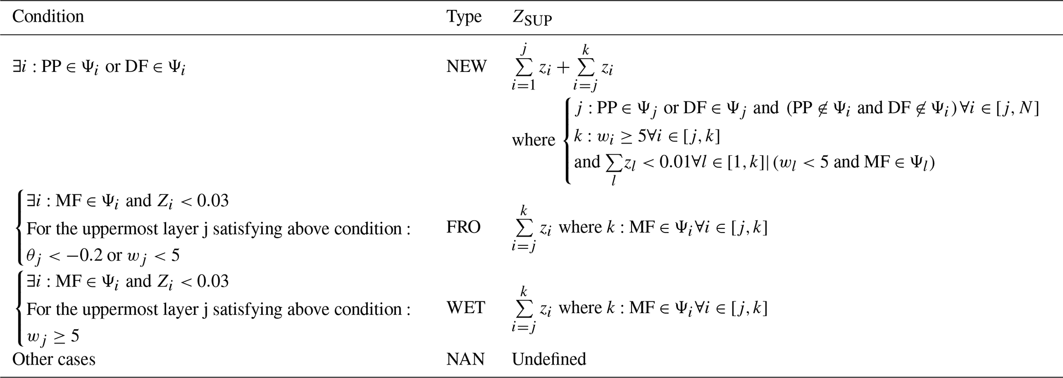
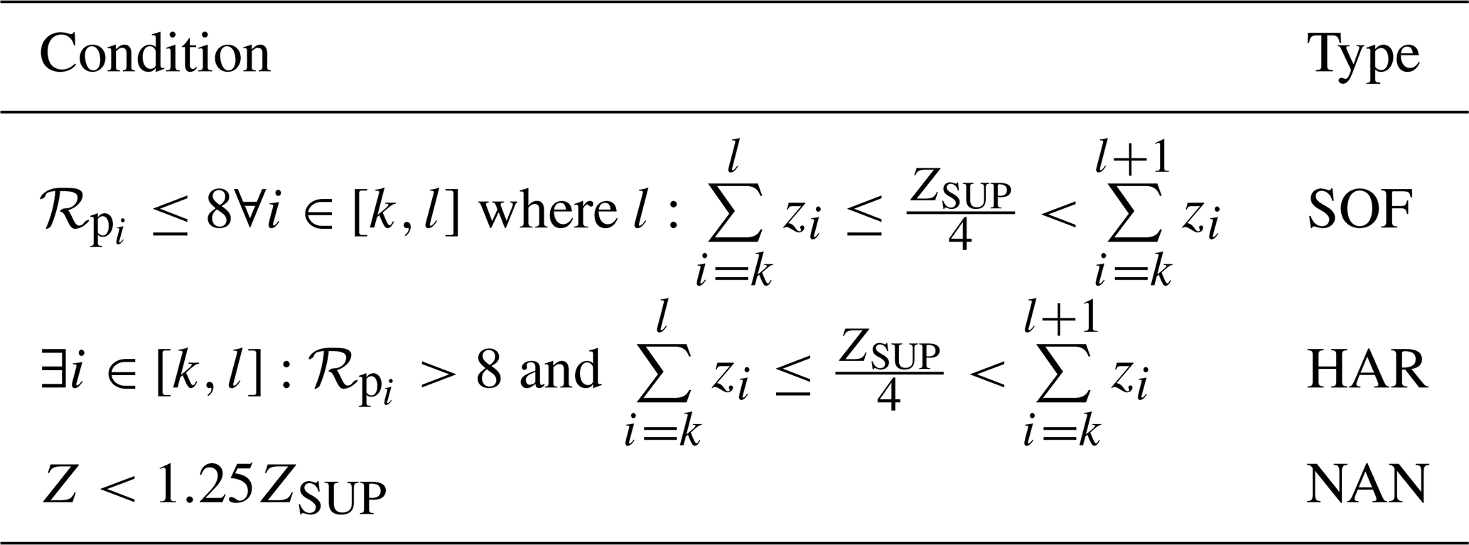
H2 Classification of avalanche situations

The avalanche situation is classified in 6 typical classes: NEW_DRY (new snow, dry), NEW_WET (new snow, wet), NEW_MIX (new snow, mixed type), MEL_SUR (melting at surface), MEL_GRO (melting, not mainly at surface) and AVA_NAN if could not identify to an other type. The expert rules determining avalanche type from superior profile, inferior profile, temperature and liquid water content of layers of superior profile are described in following equation:

$$\begin{array}{}\text{(H1)}& \left\{\begin{array}{l}\mathrm{NEW}\left\{\begin{array}{l}\mathrm{If}{w}_i<\mathrm{5}\forall i|Z_i\le Z_{\mathrm{SUP}}\to \mathrm{NEW}\mathrm{\_}\mathrm{DRY}\\ \mathrm{If}{w}_i\ge \mathrm{5}\forall i|Z_i\le Z_{\mathrm{SUP}}\to \mathrm{NEW}\mathrm{\_}\mathrm{WET}\\ \mathrm{else}\to \mathrm{NEW}\mathrm{\_}\mathrm{MIX}\end{array}\right.\\ \mathrm{WET}\left\{\begin{array}{l}\mathrm{HAR}\to \mathrm{MEL}\mathrm{\_}\mathrm{SUR}\\ \mathrm{SOF}\to \mathrm{MEL}\mathrm{\_}\mathrm{GRO}\\ \mathrm{else}\left\{\begin{array}{l}\mathrm{If}{w}_i\ge \mathrm{5}\forall i|\mathrm{0.1}<Z_i\le Z_{\mathrm{SUP}}\to \mathrm{MEL}\mathrm{\_}\mathrm{GRO}\\ \mathrm{else}\to \mathrm{MEL}\mathrm{\_}\mathrm{SUR}\end{array}\right.\end{array}\right.\\ \mathrm{FRO}\left\{\begin{array}{l}\mathrm{If}{\mathcal{H}}_{\mathrm{nat}}=\mathrm{0}\to \mathrm{AVA}\mathrm{\_}\mathrm{NAN}\\ \mathrm{else}\left\{\begin{array}{l}\mathrm{HAR}\to \mathrm{MEL}\mathrm{\_}\mathrm{SUR}\\ \mathrm{SOF}\to \mathrm{MEL}\mathrm{\_}\mathrm{GRO}\\ \mathrm{else}\left\{\begin{array}{l}\left[\begin{array}{rl}{\displaystyle }& {\displaystyle }\mathrm{If}{w}_k\ge \mathrm{5}\mathrm{for}k|Z_k=Z_{\mathrm{SUP}}\\ {\displaystyle }& {\displaystyle }\mathrm{and}{\sum }_{i=j}^k{z}_i>{\displaystyle \frac{Z_{\mathrm{SUP}}}{\mathrm{3}}}\mathrm{where}j|Z_{j-\mathrm{1}}<\mathrm{0.1}<Z_j\end{array}\right]\to \mathrm{MEL}\mathrm{\_}\mathrm{GRO}\\ \mathrm{else}\to \mathrm{MEL}\mathrm{\_}\mathrm{SUR}\end{array}\right.\end{array}\right.\end{array}\right.\\ \mathrm{NAN}\to \mathrm{AVA}\mathrm{\_}\mathrm{NAN}\end{array}\right..\end{array}$$

H3 Accounting for the temporal evolution in natural hazard index

• If at time t, superior profile is NEW but avalanche type is not NEW_MIX and if between t−Δt_M and t, avalanche type has remained unchanged and Z and Z_SUP have decreased, then ℋ_nat is updated from Table H3. The same rule is applied if avalanche type is NEW_MIX but only if the continuous wet thickness $Z_{\mathrm{W}}=\sum _{i=\mathrm{0}}^{n_W}{z}_i$ where $n_{\mathrm{W}}|w_i>\mathrm{5}\forall i\in [\mathrm{1},n_{\mathrm{W}}]$ has decreased or remained constant since t−Δt_M.

• If superior profile is WET or FRO at t and at t−Δt_M and Z−Z_SUP has not reduced by more than 0.05 m between t−Δt_M and t:

  • If ℋ_nat=3 then it is reduced to 2

  • If superior profile is WET and ${\mathcal{H}}_{\mathrm{nat}}\left(t\right)\in [\mathrm{4},\mathrm{5}]$ then:

    • If ${\mathcal{H}}_{\mathrm{nat}}(t-\mathrm{\Delta }{t}_{\mathrm{M}})\in [\mathrm{3},\mathrm{4},\mathrm{5}]$, then ℋ_nat(t)=3

    • If ${\mathcal{H}}_{\mathrm{nat}}(t-\mathrm{\Delta }{t}_{\mathrm{M}})=\mathrm{1}$, then ℋ_nat(t)=1.

Table H3 Update of ℋ_nat depending on ℋ_nat(t) as assessed from Eq. (157) and from its value at previous output time step ℋ_nat(t−Δt_M). – represents an undefined value.

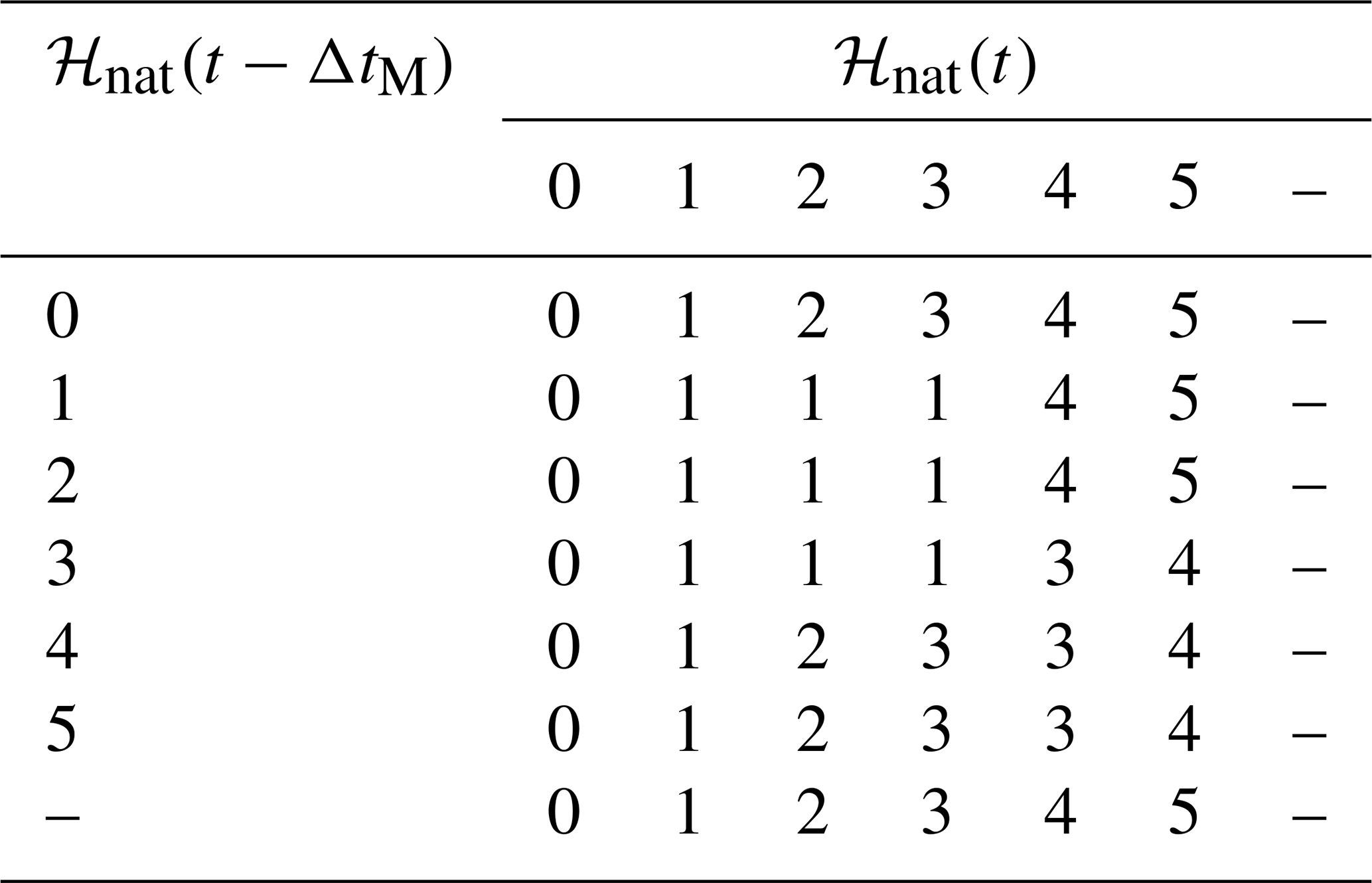
H4 Equivalent natural hazard index

In Eq. (159), ℋ_eq is designed to account for natural hazards in the assessment of the accidental hazard index. It is defined by:

$$\begin{array}{}\text{(H2)}& {\displaystyle }\left\{\begin{array}{l}\mathrm{if}Z\ge \mathrm{0.2}\mathrm{m}\left\{\begin{array}{ll}\mathrm{If}{\mathcal{H}}_{\mathrm{nat}}\ge \mathrm{4}:& {\mathcal{H}}_{\mathrm{eq}}=\mathrm{3}\\ \mathrm{If}\mathrm{2}\le {\mathcal{H}}_{\mathrm{nat}}<\mathrm{4}:& {\mathcal{H}}_{\mathrm{eq}}=\mathrm{2}\\ \mathrm{If}{\mathcal{H}}_{\mathrm{nat}}=\mathrm{1}:& {\mathcal{H}}_{\mathrm{eq}}=\mathrm{1}\end{array}\right.\\ \mathrm{else}:& {\mathcal{H}}_{\mathrm{eq}}=\mathrm{1}\end{array}\right..\end{array}$$

Appendix I: Overview of simulation results with the ESM-SnowMIP dataset

This appendix illustrates the application of Crocus 3.0.2 at the 10 ESM-SnowMIP reference sites. In-situ meteorological forcing and evaluation dataset are available from Ménard et al. (2019). Simulations are performed with default physical options as defined in Table 1 except for the 3 BERMS forest sites (Saskatechewan, Canada) where the coupling with MEB is activated. Default values are used for all adjustable parameters as defined in Appendix K5 except for z_a and z_u which are adjusted following the site-specific metadata (Ménard et al., 2019). Simulations are compared with observations of snow depth, snow water equivalent, albedo and surface temperature at two alpine sites where all observations are available (Col de Porte, 1325 m, France, Fig. I1, and Weissfluhjoch, 2540 m, Switzerland, Fig. I2) and only with snow depth for the 8 other sites (Figs. I3–I10). The illustrations show the ability of the model to simulate contrasted stratigraphies between wet sites dominated by Melt Forms (Figs.  refcdp and I7), cold sites dominated by Faceted Crystals or Depth Hoar (Figs. I3–I5 and I9), and high-elevation sites with thick and often dry snowpacks dominated by Rounded Grains with only thin layers of Faceted Crystals (Figs. I2, I8 and I10). Table I1summarizes the model skill with scores computed following Lafaysse et al. (2017) on the 7-year periods selected for illustration. They do not exhibit any systematic bias on the evaluated variables and errors in the magnitude of other snow models (Menard et al., 2021). These results can be considered as a benchmark of the model skill in various environment and climate conditions. This benchmark can be useful to assess the impact of future model developments.

Table I1 Scores of Crocus 3.0.2 simulations forced and evaluated by the ESM-SnowMIP dataset. Missing cells correspond to unavailable observations in the dataset. N is the number of available data considered to compute the scores. 7-year evaluation periods for all sites: 2007–2014 for Col de Porte (cdp), Weissfluhjoch (wfj), Sapporo (sap), Senator Beck (snb), Sodankyla (sod), Swamp Angel (swa); 2003–2010 for BERMS old aspen (oas), old black spruce (obs) and old jack pine (ojp); 2001–2008 for Reynolds Mountain East (rme), as in the associated illustrations (Figs. I1–I10).

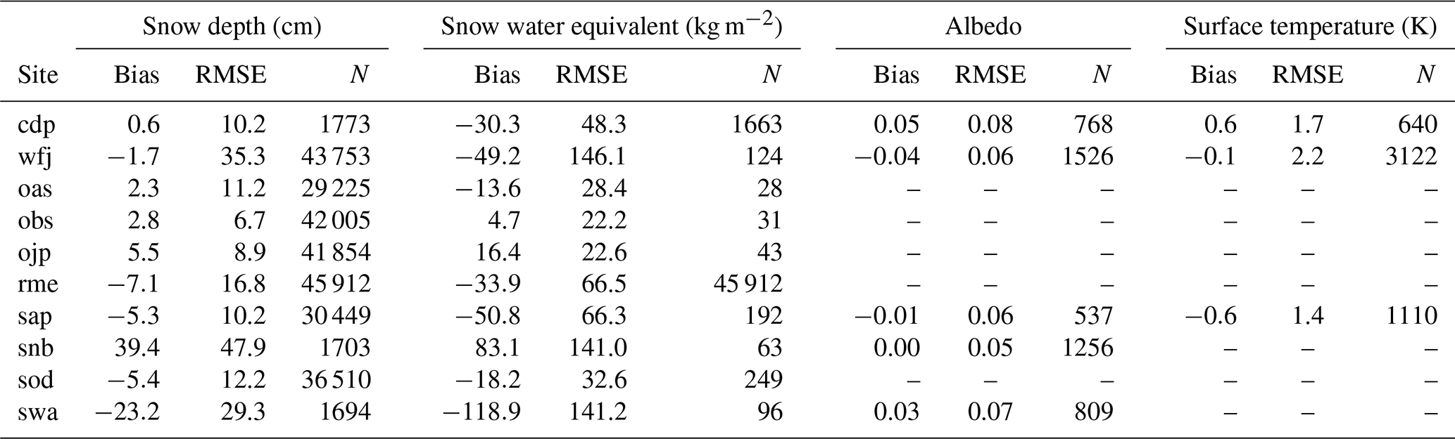
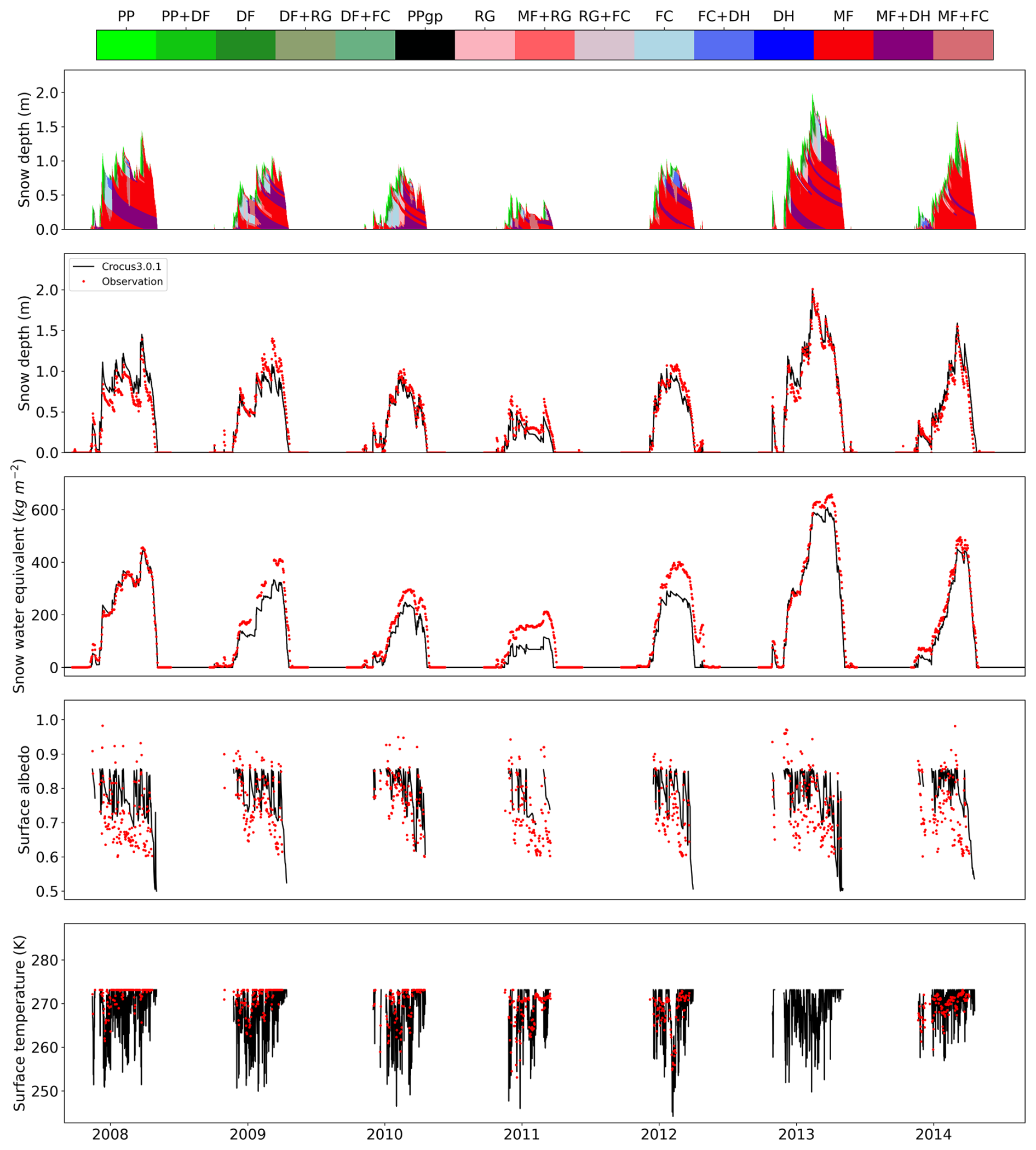
Figure I1 Illustration of Crocus simulation with ESM-SnowMIP dataset. Snow grain type, snow depth, snow water equivalent, snow surface albedo, snow surface temperature. Col de Porte, France, 2007–2014.

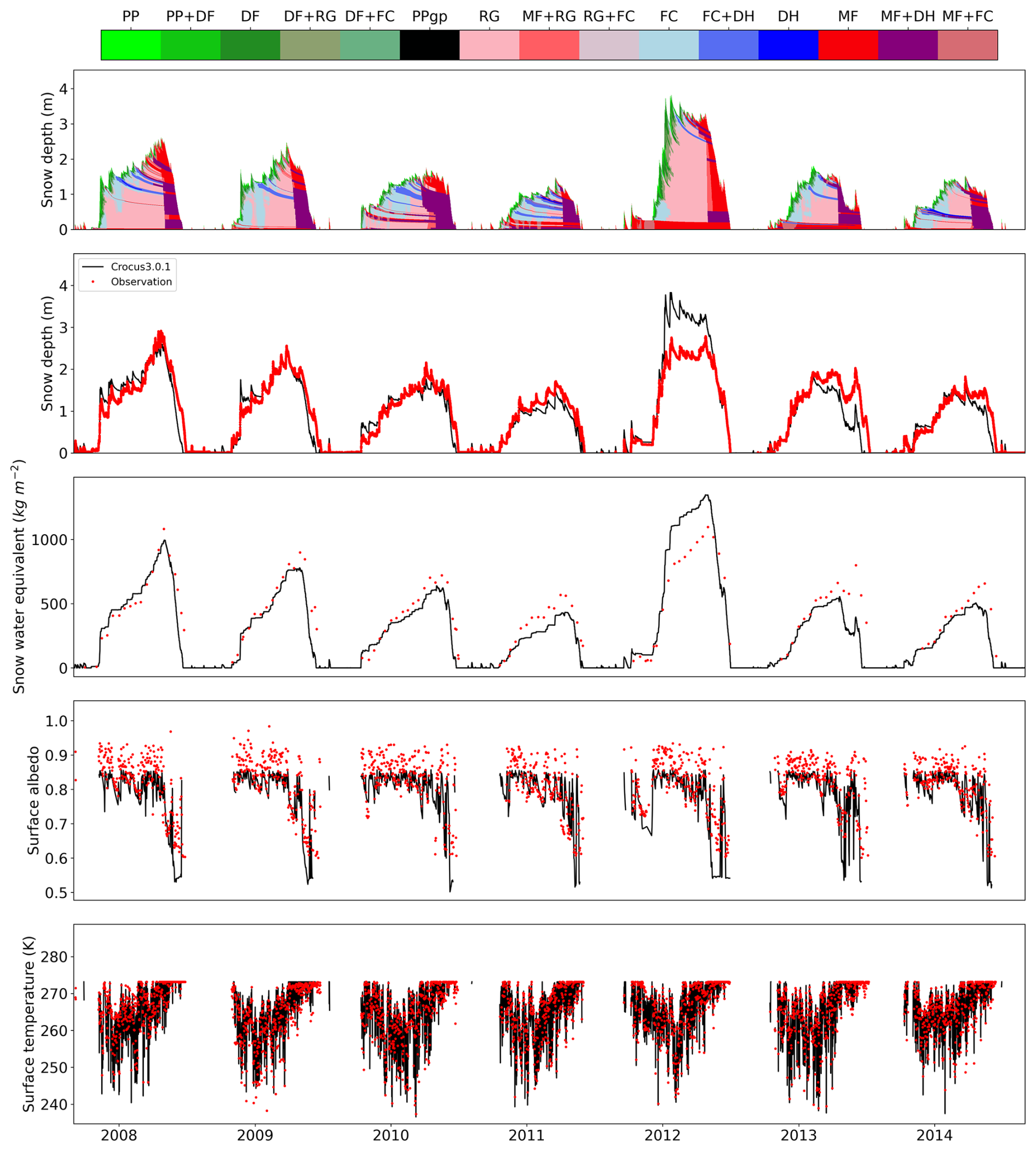
Figure I2 Illustration of Crocus simulation with ESM-SnowMIP dataset. Snow grain type, snow depth, snow water equivalent, snow surface albedo, snow surface temperature. Weissfluhjoch, Switzerland, 2007–2014.

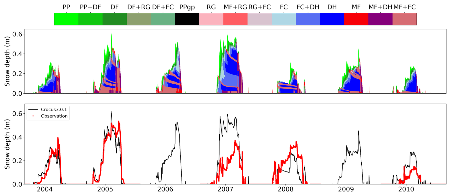
Figure I3 Illustration of Crocus simulation with ESM-SnowMIP dataset. Snow grain type, snow depth. BERMS Old Aspen, Saskatchewan, Canada, 2007–2014.

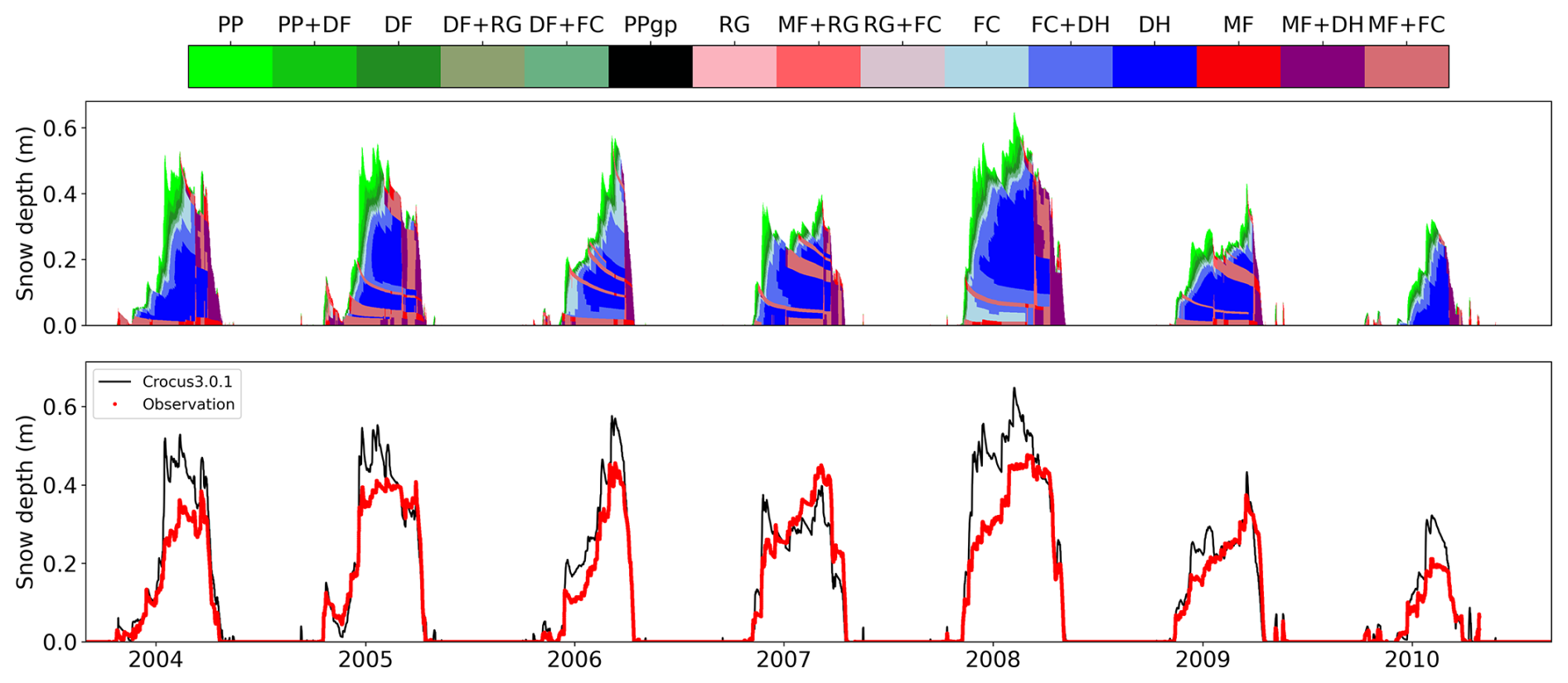
Figure I4 Illustration of Crocus simulation with ESM-SnowMIP dataset. Snow grain type, snow depth. BERMS Old Black Spruce, Saskatchewan, Canada, 2007–2014.

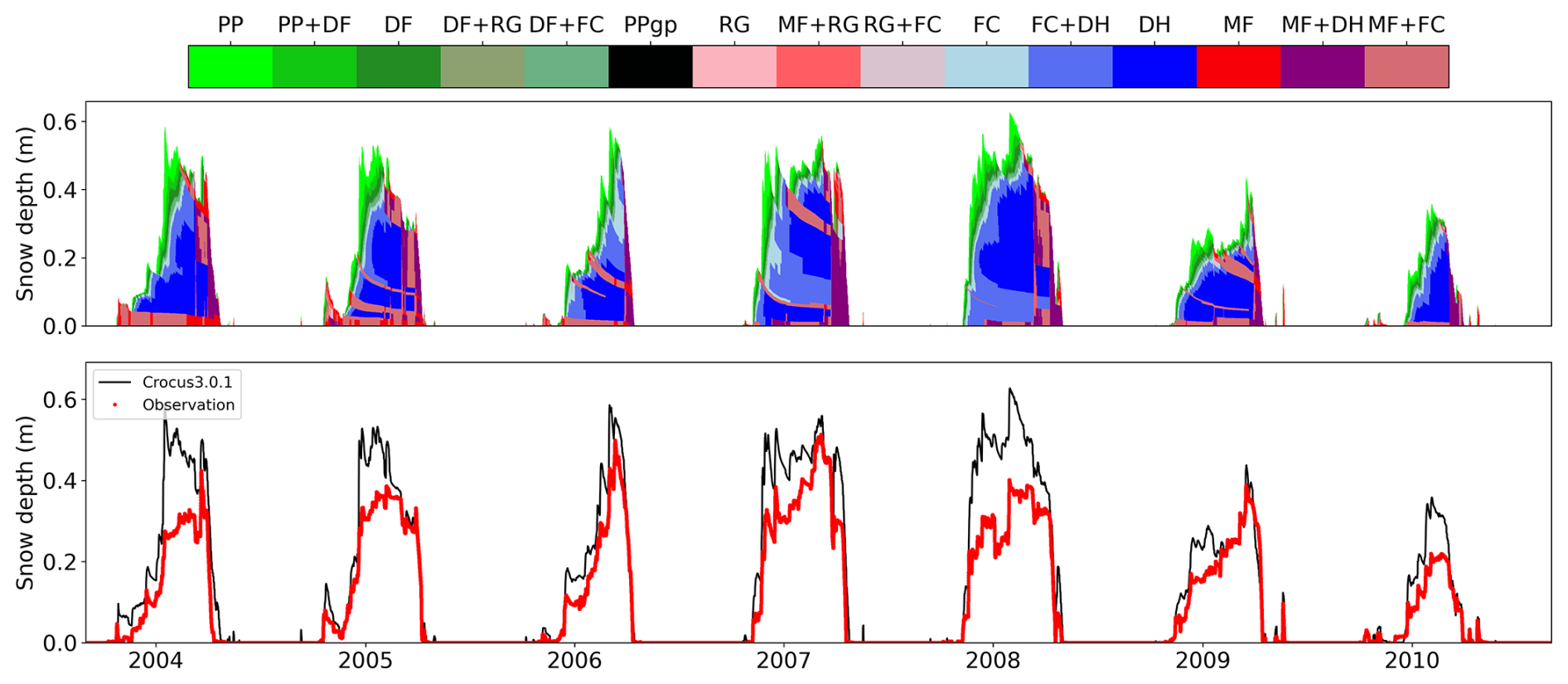
Figure I5 Illustration of Crocus simulation with ESM-SnowMIP dataset. Snow grain type, snow depth. BERMS Old Jack Pine, Saskatchewan, Canada, 2007–2014.

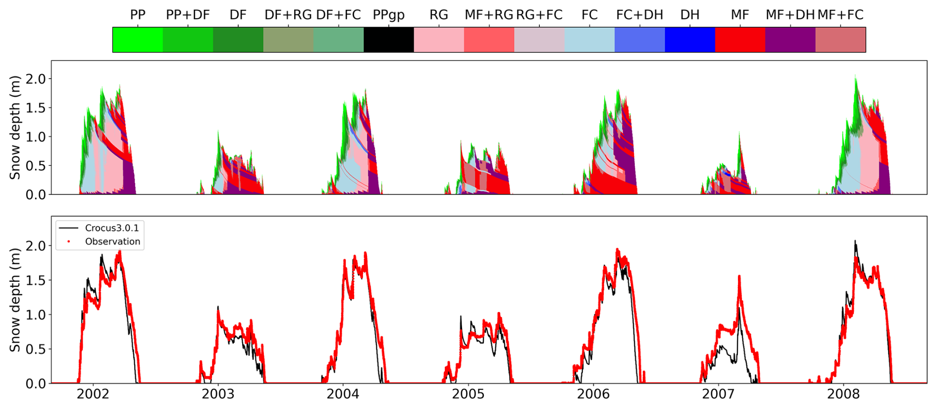
Figure I6 Illustration of Crocus simulation with ESM-SnowMIP dataset. Snow grain type, snow depth. Reynolds Mountain East, Idaho, USA, 2007–2014.

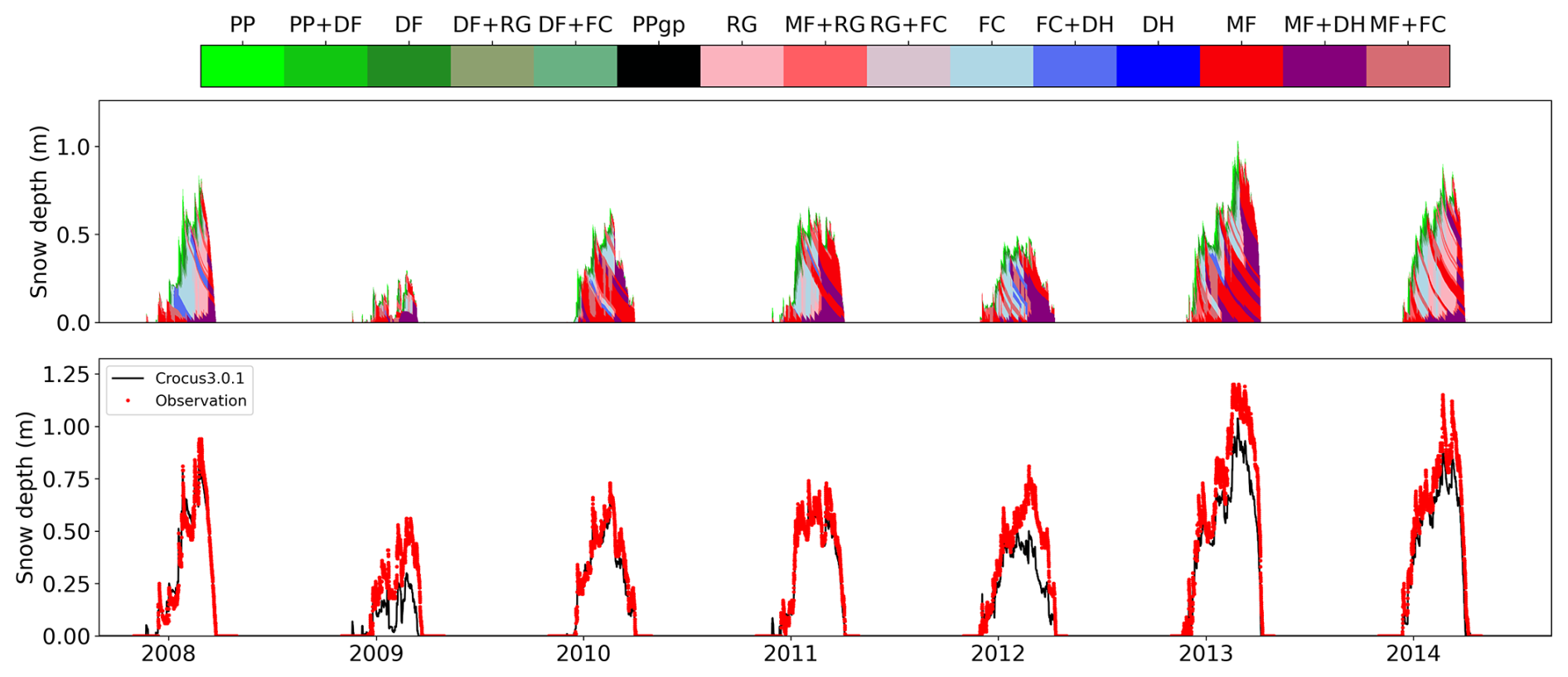
Figure I7 Illustration of Crocus simulation with ESM-SnowMIP dataset. Snow grain type, snow depth. Sapporo, Japan, 2007–2014.

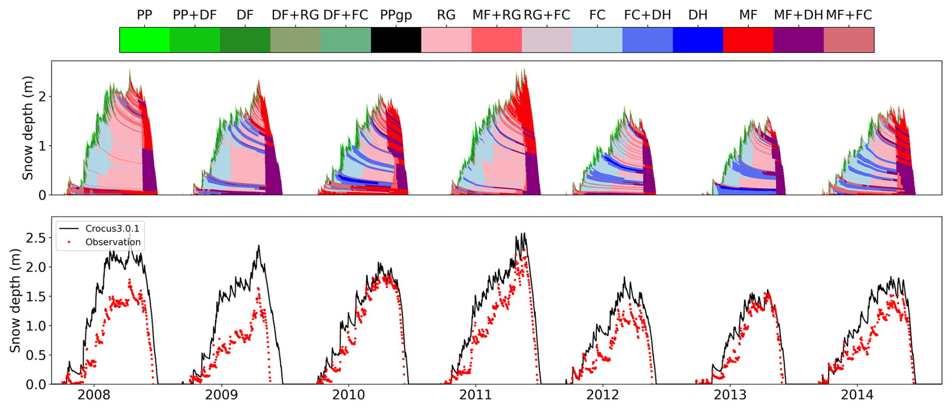
Figure I8 Illustration of Crocus simulation with ESM-SnowMIP dataset. Snow grain type, snow depth. Senator Beck, Colorado, USA, 2007–2014.

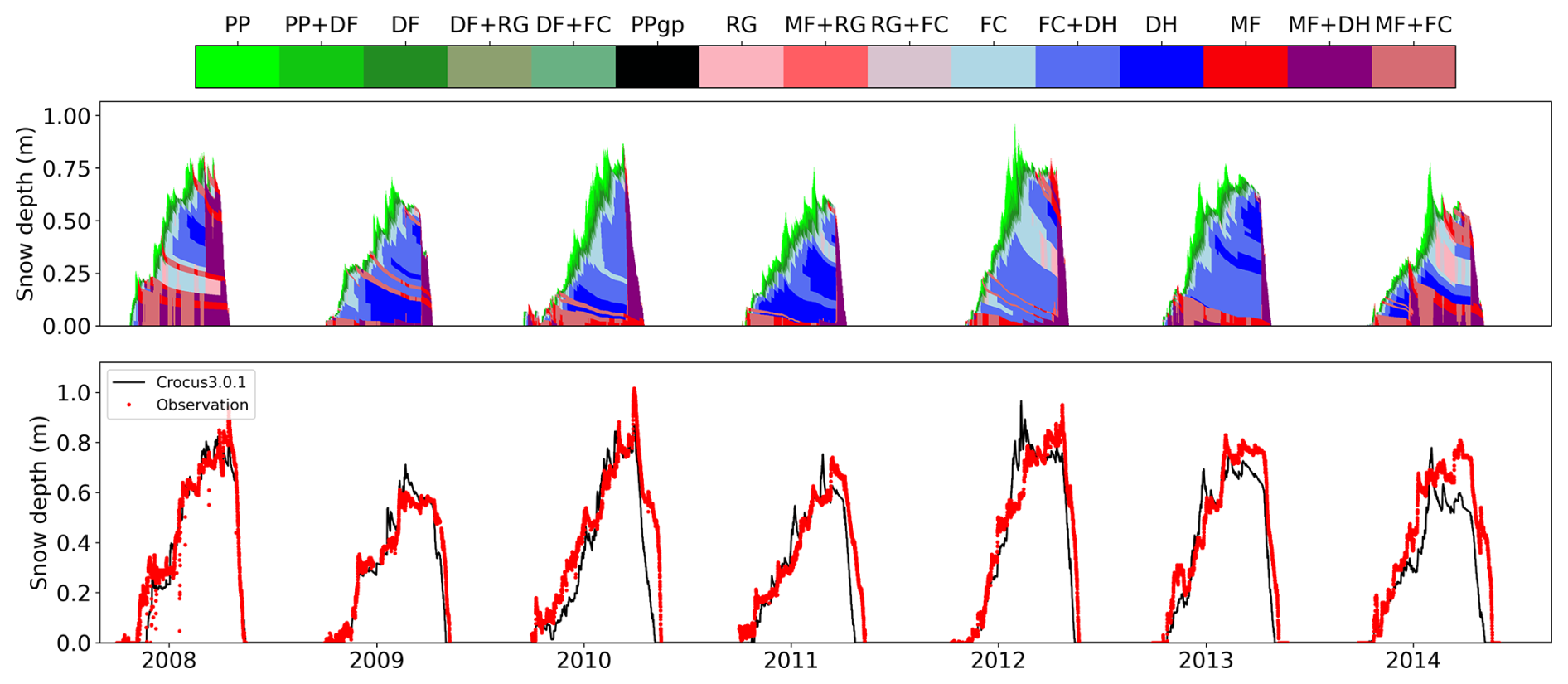
Figure I9 Illustration of Crocus simulation with ESM-SnowMIP dataset. Snow grain type, snow depth. Sodankylä, Finland, 2007–2014.

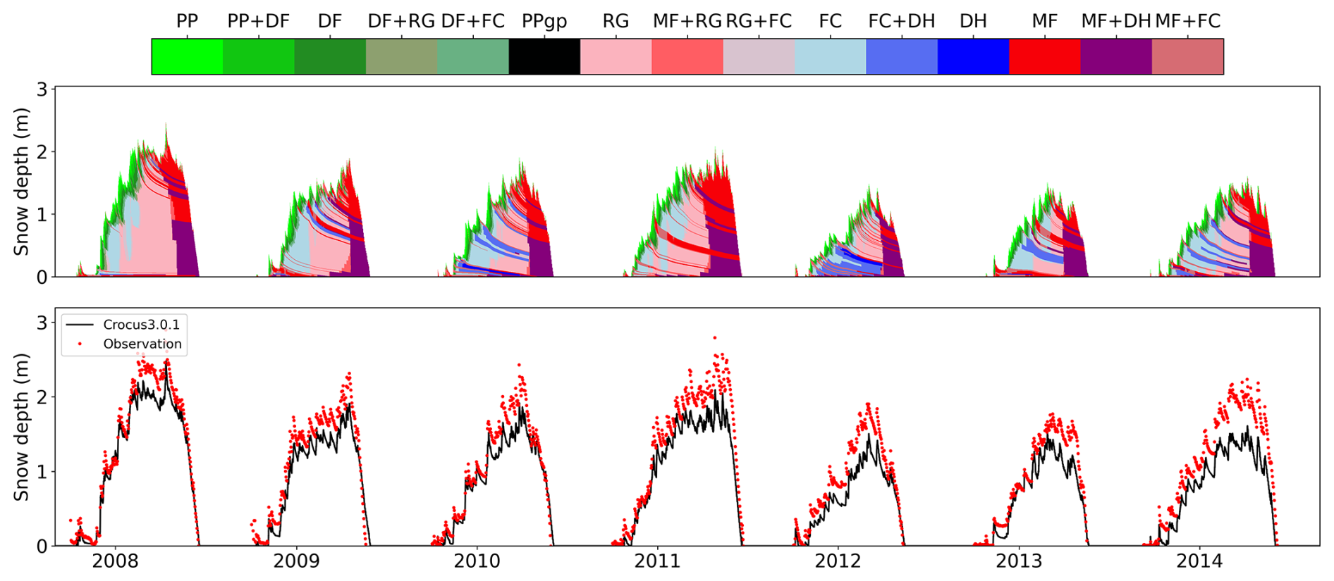
Figure I10 Illustration of Crocus simulation with ESM-SnowMIP dataset. Snow grain type, snow depth. Swamp Angel, Colorado, USA, 2007–2014.

Appendix J: Numerical efficiency of loops

All equations of this paper must be applied iteratively over all simulation points and often over all snow layers. The variable number of active snow layers N between points introduces a spatial dependence of the boundary of the loop iterator operating on snow layers. Furthermore, the maximum number of snow layers also depends on time. Several options are possible to implement these specificities, in the context where in SURFEX the leftmost dimension of arrays represent the spatial dimension, which is also the fastest varying dimension in Fortran with continous memory storage. Without extended analyses of their numerical impact, two options were implemented in previous versions of the code. A compressed-index form (CINDX, Algorithm 1) where the loop over snow layers is inside the loop over points had been chosen by Vionnet et al. (2012) in most parts of the code. This option minimizes the number of iterations and operations as the boundary of the snow layer iterator can vary between points and dates. However, the successive accesses to the values of the arrays are not performed continuously relatively to the memory storage involving more expensive memory accesses and preventing the vectorization of computations. A full iteration with condition (FCOND, Algorithm 2) had been chosen in other parts including the heat diffusion and the TARTES optical scheme. This option does not minimize the number of iterations but still minimizes the number of operations and allows continuous memory accesses. However, it adds a potentially expensive conditional statement which still prevents vectorization. Other options could be considered. For instance, a full iteration with a predefined mask (FMASK, Algorithm 3) allows continuous memory access and vectorization. However, it adds operations on empty layers so that the interest of this approach is expected to increase with the matrices density. Note also that some operations such as divisions must be secured with this approach to avoid floating point exceptions on empty layers.

Algorithm J1 Loops with compressed index (CINDX): illustration for the computation of vertical gradient.

for $p\in [\mathrm{1},N_{\mathrm{p}}]$ do

for $i\in [\mathrm{1},N(p)-\mathrm{1}]$ do

$\mathcal{G}(p,i)=\mathrm{2}\frac{T(p,i)-T(p,i+\mathrm{1})}{z(p,i)+z(p,i+\mathrm{1})}$

end for

end for

Algorithm J2 Loops with full iteration with condition (FCOND): illustration for the computation of vertical gradient.

for $i\in \left[\mathrm{1},N_{\max }-\mathrm{1}\right]$ do

for $p\in \left[\mathrm{1},N_{\mathrm{p}}\right]$ do

if $i\le N\left(p\right)-\mathrm{1}$ then

$\mathcal{G}(p,i)=\mathrm{2}\frac{T(p,i)-T(p,i+\mathrm{1})}{z(p,i)+z(p,i+\mathrm{1})}$

end if

end for

end for

Algorithm J3 Loops with full iteration with mask (FMASK): illustration for the computation of vertical gradient. MASK is a precomputed array with 1 values for defined snow layers (i≤N) and 0 for undefined layers (i>N).

for $i\in \left[\mathrm{1},N_{\max }-\mathrm{1}\right]$ do

for $p\in \left[\mathrm{1},N_{\mathrm{p}}\right]$ do

$\mathcal{G}(p,i)=\mathrm{2}\frac{T(p,i)-T(p,i+\mathrm{1})}{z(p,i)+z(p,i+\mathrm{1})}\times \mathrm{MASK}(p,i)$

end for

end for

Comparing the numerical efficiency of the whole model with these different options would represent a considerable amount of work because it would need to code all the model loops with these options. Therefore, the efficiency of these different options were only compared on simple test cases with random initialization values: the sum of a quantity over the vertical dimension (i.e. computation of total snow depth Z), the computation of the vertical gradient of a quantity (i.e. Eq. 41), the solving of a linear system with a tridiagonal matrix (i.e. Eq. 105), and finally the series of Equations to represent metamorphism (Sect. 2.4.5). The obtained results are presented in Table J1 and exhibit a large variability depending on the operations and matrix filling. Although, the initially implemented compressed-index method was found to be more efficient for all operations in the case of sparse matrices (N=12 layers), the efficiency is highly deteriorated in case of dense matrices (N closer to 50) probably due to the discontinuous accesses to memory. The full iteration with condition has the best efficiency for simple operations. The full iteration with mask improves the efficiency of the inversion of tridiagonal matrix compared to other methods but deteriorates the efficiency of the complex metamorphism routine with numerous conditional statements. Finally, the whole code was homogenized using a full iteration with condition (FCOND) allowing continous memory accesses and presenting more stable computing times in the most common cases. We recommend that future developments follow the same approach, unless a dedicated efficiency performance test is able to demonstrate that an added value is obtained with another method for a specific and expensive algorithm.

Table J1 Comparison of computing time of loops based on compress-index form (CINDX), a full iteration with condition (FCOND), and a full iteration with mask (FMASK), for 4 types of operations: sum over the layer dimension; Computation of vertical gradients; solving of a linear system with tridiagonal matrix (Eq. 107); and the whole metamorphism routine (Sect. 2.4.5). Tests were applied with 3 different densities of matrices (12 layers/50; 50 layers/50 ; or random values between 12 and 50 layers/50) and with two lengths of the spatial dimension (100 and 4000 points, adjusting the number of iterations to have the same number of computations). Tests are performed with Intel^® Fortran Compiler 18.0.5 and O₂ optimization level on one physical core of a 2.2 GHz AMD © Rome computing node. For each test, the bold value emphasizes the optimal computing time among the 3 forms of loops iterations.

Appendix K: Symbols and units

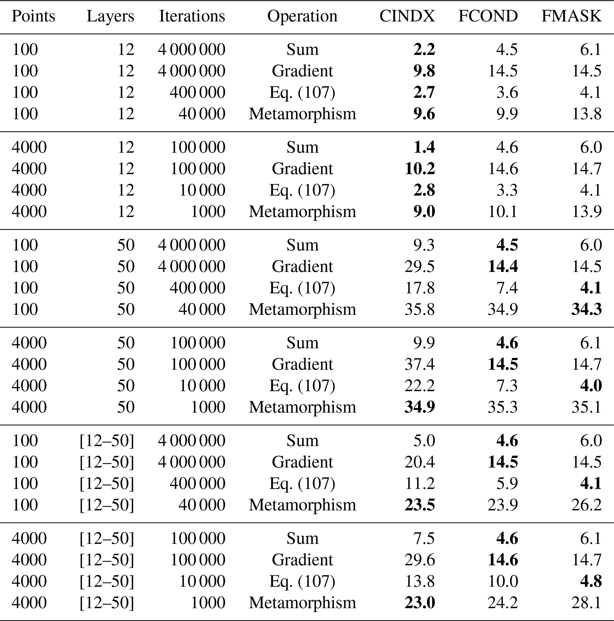
K1 Indexes

Symbol	Description
i	snow layer, i=1 refers to the surface layer, increasing indexes going down
j	type of Light-Absorbing Particles
k	spectral band for solar radiation
p	simulation point (spatial dimension)

K2 Variables

Symbol	Units	Description
Ai	days	Age of snow layer i
CH	–	Exchange coefficient for turbulent fluxes
di	m	Optical diameter of layer i
dn	m	Optical diameter of new snow
dSP	m	Optical diameter of solid precipitation
dBS	m	Optical diameter of blowing snow
$D(i,i+\mathrm{1})$	–	Similarity criteria between layers i and i+1
𝒟i	–	Driftability index of layer i
fi	kg m−2	Mass of melting for layer i during a time step
EFRZ	W m−2	Energy released at the surface by freezing of supercooled rain
Ei	W m−2	Energy of phase change for layer i
$E_{{\mathrm{f}}_i}$	W m−2	Energy available for fusion in layer i
$E_{{\mathrm{r}}_i}$	W m−2	Energy available for refreezing in layer i
$E_{k_i}$	W m−2	Absorbed solar radiation by layer i for spectral band k
ℱi	kg m−2	Liquid water flow between layer i and i+1 during a time step
𝒢i	K m−1	Vertical temperature gradient in layer i
Gi	W m−2	Global heat flux between layers i and i−1
hi	–	Historical tracker of layer i
H	W m−2	Surface turbulent sensible heat flux
Hi	J m−2	Enthalpy of layer i
ℋnat	0–5	Natural avalanche hazard index of the simulated snow profile
ℋacc	0–3	Accidental avalanche hazard index of the simulated snow profile
li	kg m−2	Mass of liquid water of layer i
Ki	W m−2	Conduction heat flux between layers i and i−1
LE	W m−2	Surface turbulent latent heat flux
linf, lsup	–	Adjacent layers minimizing the penalty criteria
LW↓	W m−2	Incoming atmospheric longwave radiation
mi	kg m−2	Total mass of layer i
mn	kg m−2	Mass of new snow
mSP	kg m−2	Mass of new solid precipitation
mBS	kg m−2	Mass of new blowing snow
mSM	kg m−2	Mass of new machine-made snow
MX	kg m−2	Mass of snow more recent than X days
ℳi,j	kg m−2	Mass of Light-Absorbing Particles of type j in layer i
MOBi	–	Mobility index of layer i
N	–	Number of active layers
Np	–	Number of simulation points
nX	–	Number of layers more recent than X days
nr	–	Number of refrozen layers at the surface
nw	–	Number of wet layers at the surface
𝒫r	kg m−2 s−1	Rainfall flux
𝒫s	kg m−2 s−1	Snowfall flux
Ps	Pa	Atmospheric pressure at surface
$P(i,i+\mathrm{1})$	–	Penalty criteria for aggregation between layers i and i+1
qa	kg kg−1	Air specific humidity at reference height za
qsat(T,Ps)	kg kg−1	Saturation specific humidity for temperature T and pressure Ps
ri	kg m−2	Mass of refrozen water for layer i during a time step
Ri	W m−2	Shortwave radiative flux between at the interface between layers i and i+1
Ri	–	Richardson number
${\mathcal{R}}_{{\mathrm{p}}_i}$	kgf	Penetration resistance of layer i
${\mathcal{R}}_{{\mathrm{s}}_i}$	kgf dm−2	Shear resistance of layer i
si	kg m−2	Mass of solid phase of layer i
Si	–	Sphericity of layer i
Sn	–	Sphericity of new snow
SSP	-	Sphericity of solid precipitation
SBS	–	Sphericity of blowing snow
${\mathcal{S}}_{{\mathrm{nat}}_i}$	–	Stability index of layer i for natural avalanche release
${\mathcal{S}}_{{\mathrm{acc}}_i}$	–	Stability index of layer i for accidental avalanche release
SSAi	m2 kg−1	Specific Surface Area of snow layer i

Symbol	Units	Description
SWDIR↓	W m−2	Incoming direct solar shortwave radiation
SWDIF↓	W m−2	Incoming diffuse solar shortwave radiation
SW↓	W m−2	Incoming total solar shortwave radiation
SWk↓	W m−2	Incoming spectral shortwave radiation for band k
Ta	K	Air temperature at reference height za
$T_{\mathrm{a}}^{*}$	°C	Air temperature at reference height za
$T_{\mathrm{w}}^{*}$	°C	Wet bulb air temperature
$T_{\mathrm{d}}^{*}$	°C	Dew point air temperature
Ti	K	Temperature of layer i
$T_{G_{\mathrm{1}}}$	K	Temperature of surface soil layer
U	m s−1	Wind speed at reference height zu
U>1	m s−1	Wind speed at reference height zu with a minimum threshold of 1 m s−1 for the computation of turbulent fluxes
Uz	m s−1	Wind speed at height z
𝒱SM	kg m−2 s−1	Water consumption for snow making
wi	kg m−3	Volumetric liquid water content of layer i
wi max	kg m−3	Maximum liquid water holding capacity of layer i
𝒲d,j	kg m−2 s−1	Dry deposition flux for Light-Absorbing Particles of type j
𝒲w,j	kg m−2 s−1	Wet deposition flux for Light-Absorbing Particles of type j
zi	m	Thickness of layer i
zn	m	Thickness of new snowfall
Zi	m	Depth of the bottom of layer i from the surface
ZX	m	Thickness of snow more recent than X days
Zr	m	Thickness of refrozen snow at the surface
Zw	m	Thickness of wet snow at the surface
αk	–	Spectral surface albedo for band k
${\mathit{\beta }}_{k_i}$	m−1	Absorption coefficient of solar radiation for band k and layer i
ηi	kg s−1 m−1	Viscosity of layer i
θi	°C	Temperature of layer i
Ψi	–	Grain type of layer i in the International Snow Classification
λi	W m−1 K−1	Thermal conductivity of layer i
${\mathit{\lambda }}_{G_{\mathrm{1}}}$	W m−1 K−1	Thermal conductivity of surface soil layer
$\stackrel{\mathrm{‾}}{{\mathit{\lambda }}_i}$	W m−1 K−1	Integrated thermal conductivity for layers i and i+1
μ	–	Cosine of solar zenithal angle
Πa	–	Exner function at height za
Πs	–	Exner function at the surface
ρa	kg m−3	air volumetric mass
ρi	kg m−3	Density of layer i
ρn	kg m−3	Density of new snow
ρSP	kg m−3	Density of natural snowfall
ρBS	kg m−3	Density of blowing snow
σi	Pa	Pressure of over burden snow for layer i
${\mathit{\sigma }}_{{\mathrm{GRO}}_i}$	Pa	Static stress due to snowcat for layer i
ϕi	–	Porosity of snow layer i
ϕFRZ	–	Fraction of latent heat release due to the freezing of supercooled rain consumed by the heating up to T0

K3 Fixed parameters

Symbol	Values and units	Description
Thermodynamical and physical parameters
cI	2.106×103 J kg−1 K−1	Ice specific heat capacity
cW	4.218×103 J kg−1 K−1	Liquid water specific heat capacity
cP	1.0047×103 J kg−1 K−1	Dry air specific heat capacity
$c_{{\mathrm{P}}_{\mathrm{v}}}$	1.8461×103 J kg−1 K−1	Vapor specific heat capacity
$c_{{\mathrm{P}}_{\mathrm{m}}}$	1.013×103 J kg−1 K−1	Typical moist air specific heat capacity
κVK	0.4	Von Karman constant
Lm	3.337×105 J kg−1	Latent heat of ice fusion
Lv	2.5008×106 J kg−1	Latent heat of vaporization of liquid water
Ls	2.8345×106 J kg−1	Latent heat of ice sublimation
ρI	917 kg m−3	Volumetric mass of pure ice
ρw	1000 kg m−3	Volumetric mass of liquid water
Ra	287.05967 J kg−1 K−1	Specific gas constant for dry air
Rv	461.52499 J kg−1 K−1	Specific gas constant for water vapor
T0	273.16 K	water melting point temperature assumed to be equal to the triple point value
σ	$\mathrm{5.6705}\times {\mathrm{10}}^{-\mathrm{8}}$ W m−2 K−4	Stefan–Boltzmann parameter
g	9.80665 m s−2	Gravitational acceleration
Layering parameters
Nmin	3	Minimum number of snow layers
Zmin	0.03 m	Threshold for uniform layering
Parameters for density of new snow when SNOWFALL = V12
ρmin	50 kg m−3	Minimum threshold
aρ	109 kg m−3	Regression coefficient
bρ	6 kg m−3 K−1	Regression coefficient
cρ	26 kg m${}^{-\mathrm{7}/\mathrm{2}}$ s${}^{+\mathrm{1}/\mathrm{2}}$	Regression coefficient
Parameters for density of new snow when SNOWFALL = S14
eρ	3.28	Empirical parameter
fρ	0.03	Empirical parameter
gρ	−0.36	Empirical parameter
hρ	−0.75	Empirical parameter
iρ	0.8	Empirical parameter
jρ	0.3	Empirical parameter
Parameters for density of new snow when SNOWFALL = A76
kρ	1.7 kg m−3 K−1.5	Regression coefficient
lρ	15 K	Regression coefficient
Parameters for metamorphism
sph1	11 574.07 s−1	Empirical parameter
sph2	2314.81 s−1	Empirical parameter
sph3	$\mathrm{7.2337}\times {\mathrm{10}}^{-\mathrm{7}}$ s−1	Empirical parameter
as	$\mathrm{1.1}\times {\mathrm{10}}^{-\mathrm{6}}$ m2 kg−1 s−1	Empirical parameter
bs	$\mathrm{3.1}\times {\mathrm{10}}^{-\mathrm{8}}$	Empirical parameter
ms	3.1	Empirical parameter

Symbol	Values and units	Description
Parameters for thermal conductivity when SNOWCOND = Y81
aλ	2.22 W m−1 K−1	Empirical parameter
λmin	$\mathrm{4}\times {\mathrm{10}}^{-\mathrm{2}}$ W m−1 K−1	Empirical parameter
Parameters for thermal conductivity when SNOWCOND = C11
bλ	$\mathrm{2.5}\times {\mathrm{10}}^{-\mathrm{6}}$ W m5 K−1 kg−2	Empirical parameter
cλ	$-\mathrm{1.23}\times {\mathrm{10}}^{-\mathrm{4}}$ W m2 K−1 kg−1	Empirical parameter
dλ	$\mathrm{2.4}\times {\mathrm{10}}^{-\mathrm{2}}$ W m−1 K−1	Empirical parameter
Parameters for thermal conductivity when SNOWCOND = I02
eλ	$\mathrm{2.0}\times {\mathrm{10}}^{-\mathrm{2}}$ W m−1 K−1	Empirical parameter
fλ	$\mathrm{2.5}\times {\mathrm{10}}^{-\mathrm{6}}$ W m5 K−1 kg−2	Empirical parameter
gλ	$-\mathrm{6.023}\times {\mathrm{10}}^{-\mathrm{2}}$ W m−1 K−1	Empirical parameter
hλ	−2.5425 W m−1	Empirical parameter
iλ	−289.99 K	Empirical parameter
P0	105 Pa	Empirical parameter
Parameters for solar radiation absorption when SNOWRAD = B92
γ1	0.71	Fraction of shortwave radiation in band [0.3–0.8 µm]
γ2	0.21	Fraction of shortwave radiation in band [0.8–1.5 µm]
γ3	0.08	Fraction of shortwave radiation in band [1.5–2.8 µm]
PCDP	8.7×105 Pa	Reference atmospheric pressure at Col de Porte
Parameters for solar radiation absorption when SNOWRAD = T17
λ0	400 nm	Reference wavelength for dust MAE
MAE(λ0)	110 m2 kg−1	Mass Absorption Efficiency of dust at wavelength λ0
AAE	4.1	Angström absorption exponent for dust
ρBC	1270 kg m−3	Density of black carbon
mBC	1.95–0.79 i	Refractive index of black carbon
fBC	1.638	Multiplicative factor to compute black carbon MAE
Parameters for Light-Absorbing Particles
h	0.005 m	E-folding depth of the exponential decay rate for dry deposition
Parameters for compaction when SNOWCOMP = B92
η0	7.62237×106 kg s−1 m−1	Empirical parameter
aη	0.1 K−1	Empirical parameter
bη	0.023 m3 kg−1	Empirical parameter
cη	250 kg m−3	Empirical parameter
Parameters for compaction when SNOWCOMP = S14
BS	$\mathrm{3.96}\times {\mathrm{10}}^{-\mathrm{2}}$	Empirical parameter
kS	0.18	Empirical parameter
Parameters for snow drift
aSUBL	$\mathrm{1.8}\times {\mathrm{10}}^{-\mathrm{3}}$	Empirical parameter
bSUBL	4	Empirical parameter
cSUBL	2.868	Empirical parameter
dSUBL	0.085	Empirical parameter
γSUBL	3.6	Empirical parameter

Symbol	Values and units	Description
Parameters for percolation when SNOWLIQ = B02
rmin	0.03	Mass of liquid fraction parameter in B02 parameterization
rmax	0.1	Mass of liquid fraction parameter in B02 parameterization
ρr	200 kg m−3	Density parameter in B02 parameterization
Parameters for snowmaking and grooming
𝒜SM	3300 m2	Surface area covered by a snowgun
ℒSM	0.4	Loss factor during snowmaking
dSM	$\mathrm{2.8}\times {\mathrm{10}}^{-\mathrm{4}}$ m	Optical diameter of machine-made snow
SSM	0.9	Sphericity of machine-made snow
ρGRO	450 kg m−3	Target density of groomed snow
dGRO	$\mathrm{2.6}\times {\mathrm{10}}^{-\mathrm{4}}$ m	Optical diameter of groomed snow
SGRO	0.9	Sphericity of groomed snow
Parameters for unloading
ρUN	200 kg m−3	Density of unloaded snow
dUN	$\mathrm{6}\times {\mathrm{10}}^{-\mathrm{4}}$ m	Optical diameter of unloaded snow
SUN	0.9	Sphericity of unloaded snow

K4 Physiographic parameters

Symbol	Units	Description
$z_{G_j}$	m	Depth of soil layer j
Θ	rad	Slope angle

K5 Parameters adjustable in namelist

Symbol	Default values and units	Description
Nmax	50	Maximum number of layers
Δt	900 s	model time step
ϵ	0.99	snow emissivity
Ril	0.026	Threshold on the Richardson number for the exchange coefficient parameterization
z0	10−3 m	snow roughness for momentum
$z_{{\mathrm{0}}_{\mathrm{h}}}$	10−4 m	snow roughness for heat
za	2 m	Reference height for air temperature
zu	10 m	Reference height for wind speed
${\mathit{\alpha }}_{{\mathrm{1}}_{\mathrm{G}}}$	0.38	Glacier albedo in band [0.3–0.8 µm]
${\mathit{\alpha }}_{{\mathrm{2}}_{\mathrm{G}}}$	0.23	Glacier albedo in band [0.8–1.5 µm]
${\mathit{\alpha }}_{{\mathrm{3}}_{\mathrm{G}}}$	0.08	Glacier albedo in band [1.5–2.8 µm]
ρG	850 kg m−3	Density threshold to separate snow and ice on glaciers
τa	60 d	Time constant in visible albedo parameterization
Cscav,j	0	Scavenging coefficient for Light-Absorbing Particles of type j
Tlim	269.15 K	Snowmaking: wet but temperature threshold
Ulim	4.2 m s−1	Snowmaking: wind speed threshold
day1	1 November	Snowmaking: day of beginning of the base-layer generation production period
day2	15 December	Snowmaking: day of end of the base-layer generation production period
day3	31 March	Snowmaking: day of end of the reinforcement production period
t1	0 s (= 00:00 LT)	Snowmaking: time of beginning of the base-layer generation production period
t2	86 400 s (= 12:00 LT)	Snowmaking: time of end of the base-layer generation production period
t3	64 800 s (= 18:00 LT)	Snowmaking: time of beginning of the reinforcement production period
t4	28 800 s (= 08:00 LT)	Snowmaking: time of end of the reinforcement production period
plim	150 kg m−2	Snowmaking: water use allowance for the base-layer generation production period
Zlim	0.6 m	Snowmaking: total (natural + machine-made) snow depth threshold for the reinforcement production period
ρSM	500 kg m−3	Snowmaking: machine-made snow density
aSM	−0.4377 kg K−1 s−1	Snowmaking: coefficient to compute the production potential mass of lance guns
bSM	−0.47 kg s−1	Snowmaking: coefficient to compute the production potential mass of lance guns
dayEND	4, 30, 4, 30	Grooming: month and day at which grooming is stopped (without and with snowmaking, respectively)
fGRO	1 d−1	Grooming: daily frequency of grooming