The Boundary Layer Dispersion and Footprint Model: a fast numerical solver of the Eulerian steady-state advection-diffusion equation

Understanding how greenhouse gases and pollutants move through the atmosphere is essential for predicting and mitigating their effects. We present the Boundary Layer Dispersion and Footprint Model (BLDFM), which solves the three-dimensional steady-state advection-diffusion equation in Eulerian form using a numerical approach based on the Fourier, linear shooting, and exponential integrator methods. In contrast to analytical Gaussian plume or stochastic Lagrangian models, this approach avoids several asymptotic assumptions required for closed-form solutions, such as the slender-plume approximation and power-law profiles. BLDFM relies solely on a steady-state Reynolds-averaged advection-diffusion equation with K-theory closure and horizontally homogeneous profiles that depend only on height. BLDFM is modular, decoupling the turbulence closure from the transport solver. The flexibility and modularity of the model may enable a wide range of applications, including climate impact studies, industrial emissions monitoring, and spatial flux attribution. We verify the numerical solver against an analytical test case and find excellent agreement. We also compare BLDFM with the well-established Kormann and Meixner (2001) footprint model (KM01), based on the analytical Gaussian plume. The results show overall good agreement, but some differences in the fetch of the footprints, attributed to KM01's neglect of streamwise turbulent mixing. Our results demonstrate the potential of BLDFM as a useful tool for atmospheric scientists, biogeochemists, ecologists, and engineers.

1 Introduction

Accurate quantification of atmospheric transport and mixing of trace gases, particulates and energy in the planetary boundary layer is crucial for understanding and prediction of pollutant dispersion, greenhouse gas concentrations and fluxes and surface-atmosphere exchange processes (Stull, 1988; Baldocchi, 2008). Numerical dispersion models are indispensable tools for this task: they integrate meteorological data, chemical processes and fluid dynamics to simulate how substances are transported and dispersed in the atmosphere. Such models inform a broad range of applications, from air quality management and public health risk assessments to ecosystem evaluations, climate impact studies, industrial emissions monitoring and agricultural planning (Seinfeld and Pandis, 2012). Complementary to dispersion modeling, flux footprint models are essential when interpreting measurements taken at fixed observation points, such as eddy covariance towers (Vesala et al., 2008; Aubinet et al., 2012). The footprint defines the field of view of the measurement point and represents the influence of the surface on the measured fluxes of momentum, heat, moisture or trace gases, thereby improving our understanding of how surface-atmosphere exchange processes scale from local to regional extents (Leclerc and Foken, 2014). By determining the spatial extent from which measurements arise, flux footprint models provide critical insights for applications in micrometeorology, ecology and biogeochemistry research (Schmid, 2002; Göckede et al., 2008).

In more recent years, flux footprint models gained attention for application in spatial flux attribution modeling. In this context, the aim is to map the spatial heterogeneity in fluxes of trace gases, moisture or energy around flux towers. Wang et al. (2006) demonstrated in a case study how CO₂ fluxes may be inferred by decomposing flux data from eddy covariance towers using footprint and ecosystem models. Crawford and Christen (2015) as well as Tuovinen et al. (2019) applied a similar technique in combination with environmental controls and surface land cover maps to attribute sources of measured eddy covariance fluxes of CO₂ and methane, respectively. Rey-Sanchez et al. (2022) used this approach to detect hot spots of methane. Pirk et al. (2024) exploit a Bayesian Neural Network to spatially disaggregate carbon exchange of degrading permafrost peatlands. The fidelity of these efforts depends on a precise flux footprint model that accurately associates the ground fluxes with the measured fluxes.

Conceptually, both dispersion models and footprint models are based on the transport equation governing the advection and turbulent mixing of a scalar, such as temperature, moisture, trace gas or pollutant in the atmosphere. In these models, the statistical effect of turbulent mixing on the resolved scales is commonly represented through an eddy diffusivity based on K-theory for turbulence closure, i.e. a subgrid-scale parametrization. Mathematically, the governing equation is a partial differential equation evolving the scalar in space and time, usually referred to as the advection-diffusion equation (Stockie, 2011). For the problem at hand, we must consider the typical scale for eddy covariance footprints (∼100 m) which is usually denoted as the atmospheric microscale in the planetary boundary layer. On this scale, the equation can be simplified by assuming a steady state, i.e., by neglecting the time derivative of the scalar. The steady-state assumption is standard in the eddy covariance method. It holds due to a scale separation: while a tracer is dynamically advected with the mean flow and turbulently mixed on the microscale, the temporal evolution of wind patterns causing this transport occurs, on the other hand, on the mesoscale (∼10 km).

Under a given set of assumptions, the steady-state advection-diffusion equation admits a closed-form analytical solution known as the Gaussian plume. This solution assumes a steady, spatially uniform wind field; steady, isotropic eddy diffusivity; and negligible mixing in the direction of the mean flow. Several dispersion and footprint models are based on similar (semi-)analytical formulations (Pasquill, F., 1972; Schuepp et al., 1990; Lin and Hildemann, 1997; Kormann and Meixner, 2001; Moreira et al., 2005; Krapez and Ky, 2023). However, the asymptotic assumptions necessary to derive analytical closed-form solutions can be quite restrictive, as they are only valid for a limited range of meteorological conditions.

Alternatively, reformulating the advection-diffusion equation such that the frame of reference follows an individual flow parcel yields the Lagrangian specification of the transport problem. The trajectories of the Lagrangian parcels are often modeled stochastically (Hsieh et al., 2000; Kljun et al., 2002, 2015). It should be noted that in stochastic Lagrangian footprint models, initially well-mixed tracers will not always, unconditionally, remain so (Thomson, 1987). This so-called “well-mixed condition” can thus be used as a quality measure for the performance of a stochastic Lagrangian model. However, most of the models that fulfill the well-mixed condition are restricted to only one given turbulence regime (Vesala et al., 2008).

Instead of parametrizing turbulent mixing by eddy diffusivity, Large Eddy Simulations (LES) resolve the relevant turbulent scales such that advection becomes the dominant transport mechanism for the scalar (Steinfeld et al., 2008; Cai et al., 2010; Schlutow et al., 2024). Despite their capabilities in simulating complex flows over uneven terrain in various turbulent regimes, LES of the planetary boundary layer consist of sophisticated numerical solvers of the Navier-Stokes equations and are computationally expensive.

In this paper, we propose an alternative atmospheric dispersion and footprint model applicable in the planetary boundary layer, which is based on the numerical solution of the three-dimensional advection-diffusion equation in Eulerian form. This numerical solver exploits the Fast Fourier Transform (FFT), allowing for fast and accurate computation. The numerical solution of the transport problem has the following benefits:

1. Unlike stochastic Lagrangian models, which typically satisfy the well-mixed condition only for a single turbulence regime, BLDFM is not tied to one specific regime, and atmospheric stability enters solely through the prescribed vertical profiles.

2. In contrast to analytical approaches, BLDFM avoids the asymptotic assumptions required to derive closed-form solutions, such as the slender-plume approximation and the power-law representation of the vertical profiles.

3. The accuracy of the solution depends, instead, only on the resolution. Depending on the application, the method's performance may be varied, and the resolution can be chosen to give moderately accurate results at fast computational speed or highly accurate results at moderate speed.

4. Due to its numerical nature, the solver can be implemented in a modular fashion. In particular, the turbulence closure module is separated from the transport solver, allowing for the use of various turbulence models which may be selected depending on the use case. Subsequently, we demonstrate BLDFM with the first-order Monin-Obukhov and a one-and-a-half-order closure (Stull, 1988). Higher-order schemes remain as future work.

5. By the same design, wind profiles from real-world measurements or LES may in principle be supplied directly as input, a capability we plan to exploit in future work.

We emphasize that, while BLDFM avoids the asymptotic assumptions listed above, it has a few, albeit less strict, modeling assumptions. In particular, BLDFM is built upon a steady-state Reynolds-averaged advection-diffusion equation with first-order (K-theory) turbulence closure; horizontally homogeneous mean wind and eddy diffusivity profiles that depend only on height; a prescribed lateral boundary treatment (periodic or vanishing flux); and, for the demonstrations presented here, a turbulence closure based on Monin-Obukhov Similarity Theory. These assumptions are shared with most footprint models and define the range of conditions for which BLDFM is applicable.

Figure 1 gives an overview of BLDFM's framework and the structure of this paper. Section 2 introduces and derives the novel Boundary Layer Dispersion and Footprint Model (BLDFM). Section 4 revisits Monin-Obukhov Similarity Theory for turbulence closure. In order to verify the numerical solver, the numerical solution is tested against a specific analytical solution in Sect. 5. Tests continue in Sect. 6 where the numerical error convergence of the method is analyzed. Section 7 presents a comparison of BLDFM with the widely used and well-established flux footprint model of Kormann and Meixner (2001). Some final remarks are given in Sect. 8.

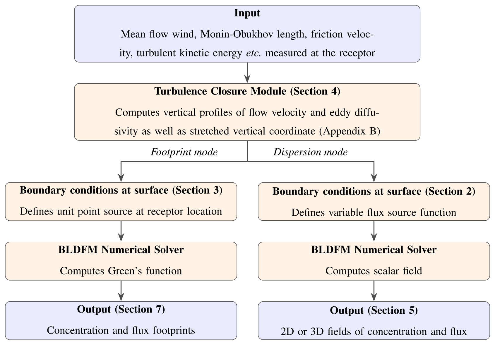
Figure 1 Overview of the BLDFM framework. Input data from the EC measurement are processed to obtain vertical profiles. Depending on the mode of operation BLDFM computes fields or footprints of concentration and flux.

2 Solving the transport equations: The Boundary Layer Dispersion and Footprint Model (BLDFM)

In this section, we derive the Boundary Layer Dispersion and Footprint Model (BLDFM). As a starting point, we consider the Reynolds-averaged steady-state advection-diffusion equation for some scalar Φ, e.g., temperature, moisture or trace gas concentration, within the planetary boundary layer,

$$\begin{array}{}\text{(1)}& {\displaystyle }{\mathit{u}}_{\mathrm{h}}\left(z\right)\cdot {\mathrm{\nabla }}_{\mathrm{h}}\mathrm{\Phi }-K_{\mathrm{h}}\left(z\right){\mathrm{\nabla }}_{\mathrm{h}}^{\mathrm{2}}\mathrm{\Phi }-{\displaystyle \frac{\partial }{\partial z}}\left(K_z\left(z\right){\displaystyle \frac{\partial \mathrm{\Phi }}{\partial z}}\right)=\mathrm{0},\end{array}$$

with flux boundary condition at the surface,

$$\begin{array}{}\text{(2)}& {\displaystyle }-K_z{\displaystyle \frac{\partial \mathrm{\Phi }}{\partial z}}=Q_{\mathrm{0}}\left({\mathit{x}}_{\mathrm{h}}\right)\text{ at }z=z_{\mathrm{0}},\end{array}$$

where ${\mathit{x}}_{\mathrm{h}}=(x,y{)}^T$ defines the horizontal coordinates in zonal and meridional direction and ${\mathit{u}}_{\mathrm{h}}=(u,v{)}^T$ is its associated horizontal vector of mean wind. The horizontal nabla operator is given by ${\mathrm{\nabla }}_{\mathrm{h}}=(\partial /\partial x,\partial /\partial y{)}^T$. Superscript T denotes the transpose of a vector or matrix. Wind, as well as horizontal and vertical eddy diffusivity, K_h and K_z, depend solely on the vertical axis z. Thus, we model a steady boundary layer flow. The variable Q₀ represents the horizontally varying surface kinematic flux of the scalar Φ. It may correspond to the sensible heat flux when Φ denotes temperature or to a surface–atmosphere gas exchange flux when Φ represents a trace gas concentration such as CO₂ or methane. For the sake of generality, we associate Φ with arbitrary units ($\mathrm{a}.\mathrm{u}.$) symbolizing K, kg kg⁻¹, mol mol⁻¹ or kg m⁻³. Thus, the kinematic flux Q₀ has units of $\mathrm{a}.\mathrm{u}.\mathrm{m}{\mathrm{s}}^{-\mathrm{1}}$.

In the lateral direction, we may assume a periodic (or vanishing) solution. By this assumption, no net flux can be generated over the horizontal boundaries. Since Eq. (1) is linear and its coefficients depend only on the z-axis, we may apply the Fourier method in the horizontal direction,

$$\begin{array}{}\text{(3)}& {\displaystyle }\mathrm{\Phi }({\mathit{x}}_{\mathrm{h}},z)& {\displaystyle }=\sum _{n=-\mathrm{\infty }}^{\mathrm{\infty }}\sum _{m=-\mathrm{\infty }}^{\mathrm{\infty }}\mathit{\phi }(\mathit{\mu },z)e^{\mathrm{i}\mathit{\mu }\cdot {\mathit{x}}_{\mathrm{h}}},\text{(4)}& {\displaystyle }\text{where}\mathit{\mu }& {\displaystyle }={\left({\displaystyle \frac{\mathrm{2}\mathit{\pi }}{L_x}}n,{\displaystyle \frac{\mathrm{2}\mathit{\pi }}{L_y}}m\right)}^T,\end{array}$$

which fulfills the lateral boundary conditions by construction. Inserting the Fourier series Eq. (3) into the steady-state advection-diffusion Eq. (1) transforms the problem into a family of second-order ordinary differential equations with parameters (n,m), which may be written as

$$\begin{array}{}\text{(5)}& {\displaystyle \frac{\mathrm{1}}{K_z}}{\displaystyle \frac{\partial }{\partial z}}\left(K_z{\displaystyle \frac{\partial \mathit{\phi }}{\partial z}}\right)-{\mathit{\sigma }}^{\mathrm{2}}\mathit{\phi }=\mathrm{0}.\end{array}$$

Equation (5) constitutes an Eigenvalue Problem (EVP) with eigenvalue

$$\begin{array}{}\text{(6)}& {\displaystyle }{\mathit{\sigma }}^{\mathrm{2}}(\mathit{\mu },z)={\displaystyle \frac{K_{\mathrm{h}}\left(z\right)}{K_z\left(z\right)}}|\mathit{\mu }{|}^{\mathrm{2}}+\mathrm{i}{\displaystyle \frac{\mathrm{1}}{K_z\left(z\right)}}\mathit{\mu }\cdot {\mathit{u}}_{\mathrm{h}}(z)\end{array}$$

and boundary condition given by

$$\begin{array}{}\text{(7)}& {\displaystyle }-K_z{\displaystyle \frac{\partial \mathit{\phi }}{\partial z}}=q_{\mathrm{0}}\left(\mathit{\mu }\right)\text{ at }z=z_{\mathrm{0}}.\end{array}$$

Here, we used the definition of the Fourier coefficients of the surface flux,

$$\begin{array}{}\text{(8)}& {\displaystyle }{q}_{\mathrm{0}}\left(\mathit{\mu }\right){\displaystyle }={\displaystyle \frac{\mathrm{1}}{L_x{L}_y}}\underset{\mathrm{0}}{\overset{L_x}{\int }}\underset{\mathrm{0}}{\overset{L_y}{\int }}{Q}_{\mathrm{0}}\left({\mathit{x}}_{\mathrm{h}}\right)e^{-\mathrm{i}\mathit{\mu }\cdot {\mathit{x}}_{\mathrm{h}}}{\mathrm{d}}^{\mathrm{2}}{\mathit{x}}_{\mathrm{h}},\end{array}$$

where $[\mathrm{0},L_x]\times [\mathrm{0},L_y]$ depicts the horizontal domain.

We aim to solve the EVP numerically. Hence, we approximate the Fourier series Eq. (3) and the integrals in the definition of the Fourier coefficients Eq. (8) by finite sums, which allows for usage of Fast Fourier Transform (FFT) in the implementation.

The Fourier series generates cyclic boundaries by construction. In order to represent non-periodic fields, a halo of zero flux is used around the domain of interest, effectively increasing the computation domain. The halo must be large enough to prevent tracer material leaving one edge from entering through the opposite site. This treatment of the boundaries makes the algorithm computationally slightly more expensive, but still provides very fast calculations due to the usage of FFT.

Consider the solution to Eq. (5) on the unbounded domain $z\in [z_{\mathrm{0}},\mathrm{\infty })$. In order to constrain the solution as z→∞, we apply a version of the weak maximum principle (Evans, 2010) that states Φ must achieve its maximum at the boundary, i.e., at z=z₀. The maximum principle may be implemented by assuming the coefficients of Eq. (1) become constant above a certain height z_T. By this premise, it is possible to compute an analytical solution φ_analytic for z>z_T. The lower boundary condition of the analytical solution for z>z_T eventually becomes the upper boundary condition for the numerical solution for $z_{\mathrm{0}}\le z\le z_{\mathrm{T}}$. The general solution of Eq. (5) with constant coefficients is found to be,

$$\begin{array}{}\text{(9)}& {\displaystyle }\mathit{\phi }& {\displaystyle }=A+Bz\text{ for }(n,m)=(\mathrm{0},\mathrm{0})\text{ and}\text{(10)}& {\displaystyle }\mathit{\phi }& {\displaystyle }=C{e}^{-\mathit{\sigma }z}+D{e}^{\mathit{\sigma }z}\text{ for }(n,m)\ne (\mathrm{0},\mathrm{0}).\end{array}$$

Notice that the solution has become degenerate for $(n,m)=(\mathrm{0},\mathrm{0})$. The maximum principle requires that D=0. Hence, the analytical solution for z>z_T is

$$\begin{array}{}\text{(11)}& {\displaystyle }{\mathit{\phi }}_{\mathrm{analytic}}& {\displaystyle }=A+Bz\text{ for }(n,m)=(\mathrm{0},\mathrm{0})\text{ and}\text{(12)}& {\displaystyle }{\mathit{\phi }}_{\mathrm{analytic}}& {\displaystyle }=C{e}^{-\mathit{\sigma }z}\text{ for }(n,m)\ne (\mathrm{0},\mathrm{0}).\end{array}$$

Taking the aforementioned considerations into account, the numerical solution of the EVP with variable coefficients as $z_{\mathrm{0}}\le z\le z_{\mathrm{T}}$ becomes a boundary value problem. For the sake of easier numerical integration, we rewrite Eq. (5) as a family of coupled first-order ordinary differential equations by substituting the vertical kinematic flux q,

$$\begin{array}{}\text{(13)}& {\displaystyle }\begin{array}{rl}{\displaystyle \frac{\partial \mathit{\phi }}{\partial z}}& {\displaystyle }=-{\displaystyle \frac{q}{K_z\left(z\right)}},\\ {\displaystyle \frac{\partial q}{\partial z}}& {\displaystyle }=\left(-\mathrm{i}\mathit{\mu }\cdot {\mathit{u}}_{\mathrm{h}}\left(z\right)-K_{\mathrm{h}}\left(z\right)|\mathit{\mu }{|}^{\mathrm{2}}\right)\mathit{\phi },\end{array}\end{array}$$

with boundary conditions as follows,

$$\begin{array}{ll}\text{(14)}& {\displaystyle }q& {\displaystyle }=q_{\mathrm{0}}\text{ at }z=z_{\mathrm{0}}\text{ for all }(n,m),{\displaystyle }\left(\begin{array}{c}\mathit{\phi }\\ q\end{array}\right)& {\displaystyle }=\left(\begin{array}{c}{\mathit{\phi }}_{\mathrm{analytic}}\\ -K_z\partial {\mathit{\phi }}_{\mathrm{analytic}}/\partial z\end{array}\right)=\left(\begin{array}{c}A+B{z}_T\\ -K_{z}B\end{array}\right)\\ \text{(15)}& {\displaystyle }& {\displaystyle }\text{ at }z=z_{\mathrm{T}}\text{ for }(n,m)=(\mathrm{0},\mathrm{0})\text{ and}{\displaystyle }\left(\begin{array}{c}\mathit{\phi }\\ q\end{array}\right)& {\displaystyle }=\left(\begin{array}{c}{\mathit{\phi }}_{\mathrm{analytic}}\\ -K_z\partial {\mathit{\phi }}_{\mathrm{analytic}}/\partial z\end{array}\right)=\left(\begin{array}{c}C{e}^{-\mathit{\sigma }{z}_{\mathrm{T}}}\\ K_z\mathit{\sigma }C{e}^{-\mathit{\sigma }{z}_{\mathrm{T}}}\end{array}\right)\\ \text{(16)}& {\displaystyle }& {\displaystyle }\text{ at }z=z_{\mathrm{T}}\text{ for }(n,m)\ne (\mathrm{0},\mathrm{0}).\end{array}$$

Let us consider both cases for (n,m) separately. The boundary conditions depend on free parameters $A,B,C$. Hence, both the ODE and the boundary conditions may be simplified.

For $(n,m)=(\mathrm{0},\mathrm{0})$, $\partial q/\partial z=\mathrm{0}$ and so the flux q=q₀ becomes constant, and the problem can be recast as an initial value problem (IVP),

$$\begin{array}{}\text{(17)}& {\displaystyle \frac{\partial \mathit{\phi }}{\partial z}}& {\displaystyle }=-{\displaystyle \frac{q_{\mathrm{0}}}{K_z\left(z\right)}},\text{(18)}& {\displaystyle }\mathit{\phi }& {\displaystyle }={\mathit{\phi }}_{\mathrm{0}}\text{ at }z=z_{\mathrm{0}}\end{array}$$

where φ₀ is a new free parameter replacing the role of A and denotes the mean concentration at the surface.

For $(n,m)\ne (\mathrm{0},\mathrm{0})$, we obtain the following simplification removing the dependency on parameters B and C,

$$\begin{array}{}\text{(19)}& {\displaystyle }\begin{array}{rl}{\displaystyle \frac{\partial \mathit{\phi }}{\partial z}}& {\displaystyle }=-{\displaystyle \frac{q}{K_z\left(z\right)}},\\ {\displaystyle \frac{\partial q}{\partial z}}& {\displaystyle }=\left[-\mathrm{i}\mathit{\mu }\cdot {\mathit{u}}_{\mathrm{h}}\left(z\right)-K_{\mathrm{h}}\left(z\right)|\mathit{\mu }{|}^{\mathrm{2}}\right]\mathit{\phi },\end{array}\end{array}$$

with boundaries

$$\begin{array}{}\text{(20)}& {\displaystyle }\begin{array}{rl}{\displaystyle }& {\displaystyle }q=q_{\mathrm{0}}\text{ at }z=z_{\mathrm{0}},\\ {\displaystyle }& {\displaystyle }-K_z\mathit{\sigma }\mathit{\phi }+q=\mathrm{0}\text{ at }z=z_{\mathrm{T}}.\end{array}\end{array}$$

Note that the upper boundary condition is converted into a Robin boundary condition.

This boundary value problem (BVP) may be solved using the linear shooting method (Lindfield and Penny, 2018). The main idea of the method is to reduce the solution of the BVP to solving two IVPs with arbitrary but linearly independent initial values and reconstruct the BVP solution by a linear combination of the two IVP solutions, allowing for the utilization of standard numerical IVP solvers.

Let (φ₁,q₁)^T be the solution of the initial value problem given by the system of ordinary differential equations (ODEs) Eq. (19) and the initial condition (1, 0)^T at z=z₀. Similarly, let (φ₂,q₂)^T be the solution of the initial value problem with initial condition (0, q₀)^T at z=z₀. The solution to the original boundary value problem at the measurement (receptor) height z_M<z_T, given by Eqs. (19) and (20), is a linear combination of the two solutions of the initial value problems,

$$\begin{array}{}\text{(21)}& {\displaystyle }& {\displaystyle }\left(\begin{array}{c}\mathit{\phi }\left(z_{\mathrm{M}}\right)\\ q\left(z_{\mathrm{M}}\right)\end{array}\right)=\mathit{\alpha }\cdot \left(\begin{array}{c}{\mathit{\phi }}_{\mathrm{1}}\left(z_{\mathrm{M}}\right)\\ q_{\mathrm{1}}\left(z_{\mathrm{M}}\right)\end{array}\right)+\mathrm{1}\cdot \left(\begin{array}{c}{\mathit{\phi }}_{\mathrm{2}}\left(z_{\mathrm{M}}\right)\\ q_{\mathrm{2}}\left(z_{\mathrm{M}}\right)\end{array}\right),\text{(22)}& {\displaystyle }& {\displaystyle }\mathit{\alpha }={\displaystyle \frac{K_z\left(z_{\mathrm{T}}\right)\mathit{\sigma }\left(z_{\mathrm{T}}\right){\mathit{\phi }}_{\mathrm{2}}\left(z_{\mathrm{T}}\right)-q_{\mathrm{2}}\left(z_{\mathrm{T}}\right)}{q_{\mathrm{1}}\left(z_{\mathrm{T}}\right)-K_z\left(z_{\mathrm{T}}\right)\mathit{\sigma }\left(z_{\mathrm{T}}\right){\mathit{\phi }}_{\mathrm{1}}\left(z_{\mathrm{T}}\right)}}.\end{array}$$

Notice that the initial values were chosen–without loss of generality–to yield compact expressions for the coefficients of the linear combination, which are computed by accounting for the boundary values at z_T.

As the ODE in Eq. (19) is linear, the IVP is most effectively solved by the exponential integrator method (Hochbruck and Ostermann, 2010), which provides exact integration for the analytic case, i.e., when the coefficients are constant. The derivation of the exponential integrator can be found in Appendix A together with a faster third-order approximation. Details on the vertical discretization utilizing stretched coordinates can be found in Appendix B.

3 Green's function and footprints

In certain applications, it might be advantageous to solve a slightly altered version of the original problem Eq. (1). Equations (19) and (20) are written as follows,

$$\begin{array}{}\text{(23)}& {\displaystyle \frac{\partial G_{\mathrm{\Phi }}}{\partial z}}& {\displaystyle }=-{\displaystyle \frac{G_Q}{K_z\left(z\right)}},\text{(24)}& {\displaystyle \frac{\partial G_Q}{\partial z}}& {\displaystyle }=K_{\mathrm{h}}\left(z\right){\mathrm{\nabla }}_{\mathrm{h}}^{\mathrm{2}}{G}_{\mathrm{\Phi }}-{\mathit{u}}_{\mathrm{h}}\left(z\right)\cdot {\mathrm{\nabla }}_{\mathrm{h}}{G}_{\mathrm{\Phi }},\end{array}$$

with boundary condition

$$\begin{array}{}\text{(25)}& {\displaystyle }-K_z{\displaystyle \frac{\partial G_{\mathrm{\Phi }}}{\partial z}}=\mathit{\delta }\left(x\right)\mathit{\delta }\left(y\right)\text{ at }z=z_{\mathrm{0}}.\end{array}$$

Here, the surface flux source term was substituted with the delta distribution, which essentially represents a unit point source of infinitesimal diameter. The vector consisting of the elements G_Φ and G_Q is the Green's function of atmospheric dispersion (Finnigan, 2004), and the numerical solution of Eqs. (23–25) follows similarly from Sect. 2.

Eventually, the solution of the original problem stated in Eqs. (1) and (2) is given by the convolution of the Green's function with the actual surface flux source term Q₀, which may be written as

$$\begin{array}{}\text{(26)}& {\displaystyle }\mathrm{\Phi }({\mathit{x}}_{\mathrm{h}},z){\displaystyle }={\displaystyle \frac{\mathrm{1}}{L_x{L}_y}}\underset{\mathrm{0}}{\overset{L_x}{\int }}\underset{\mathrm{0}}{\overset{L_y}{\int }}{Q}_{\mathrm{0}}\left({\mathit{\xi }}_{\mathrm{h}}\right)G_{\mathrm{\Phi }}({\mathit{x}}_{\mathrm{h}}-{\mathit{\xi }}_{\mathrm{h}},z){\mathrm{d}}^{\mathrm{2}}{\mathit{\xi }}_{\mathrm{h}}\end{array}$$

and similarly,

$$\begin{array}{}\text{(27)}& {\displaystyle }Q({\mathit{x}}_{\mathrm{h}},z){\displaystyle }={\displaystyle \frac{\mathrm{1}}{L_x{L}_y}}\underset{\mathrm{0}}{\overset{L_x}{\int }}\underset{\mathrm{0}}{\overset{L_y}{\int }}{Q}_{\mathrm{0}}\left({\mathit{\xi }}_{\mathrm{h}}\right)G_Q({\mathit{x}}_{\mathrm{h}}-{\mathit{\xi }}_{\mathrm{h}},z){\mathrm{d}}^{\mathrm{2}}{\mathit{\xi }}_{\mathrm{h}}.\end{array}$$

Therefore, in applications where several flux source terms are present, e.g., multitracer approaches, a Green's function needs to be computed only once for a given meteorological condition. The concentration and flux fields are then computed by the convolutions Eqs. (26) and (27), which become simple sums when discretized. In summary, the approach with Green's function may be computationally much more efficient.

Notice that there is a strong connection between the Green's function and the footprint F (Vesala et al., 2008): the footprint is the reflection of the Green's function shifted to the measurement point. In terms of the Green's function, the concentration and flux footprint may be written as,

$$\begin{array}{}\text{(28)}& {\displaystyle }{F}_{\mathrm{\Phi }}({\mathit{x}}_{\mathrm{h},\mathrm{M}},z_{\mathrm{M}};{\mathit{x}}_{\mathrm{h}})& {\displaystyle }=G_{\mathrm{\Phi }}({\mathit{x}}_{\mathrm{h},\mathrm{M}}-{\mathit{x}}_{\mathrm{h}},z_{\mathrm{M}}),\text{(29)}& {\displaystyle }{F}_Q({\mathit{x}}_{\mathrm{h},\mathrm{M}},z_{\mathrm{M}};{\mathit{x}}_{\mathrm{h}})& {\displaystyle }=G_Q({\mathit{x}}_{\mathrm{h},\mathrm{M}}-{\mathit{x}}_{\mathrm{h}},z_{\mathrm{M}}),\end{array}$$

respectively.

In conclusion, BLDFM constitutes a dispersion model and a footprint model at the same time.

4 Profiles of mean wind and eddy diffusivity

We apply Monin-Obukhov's Similarity Theory (MOST) to obtain the profiles of wind u_h as well as eddy diffusivities K_h and K_z (Monin and Obukhov, 1954; Kormann and Meixner, 2001) taking atmospheric stability into account. Under MOST, the mean horizontal wind speed can be expressed as,

$$\begin{array}{}\text{(30)}& {\displaystyle }{u}_{\mathrm{h}}\left(z\right)={\displaystyle \frac{u_{\ast }}{\mathit{\kappa }}}\left(\ln \left({\displaystyle \frac{z}{z_{\mathrm{0}}}}\right)+{\mathit{\psi }}_m\left({\displaystyle \frac{z}{L}}\right)\right),\end{array}$$

and the eddy diffusivities, assuming isotropic diffusion, are given by

$$\begin{array}{}\text{(31)}& {\displaystyle }{K}_{\mathrm{h}}\left(z\right)=K_z\left(z\right)={\displaystyle \frac{\mathit{\kappa }{u}_{\ast }z}{{\mathit{\varphi }}_c(z/L)}}.\end{array}$$

The variables u_∗, z₀ and L denote the friction velocity, roughness length and Obukhov length, respectively, with L providing a measure of boundary-layer stability. These quantities are standard diagnostic variables derived from eddy covariance measurements. The parameter κ=0.4 denotes the von Kármán constant. Atmospheric stability enters the equations by the universal functions ψ_m and ϕ_c which are specified by the Businger–Dyer relationships (Businger et al., 1971; Dyer, 1974) as

$$\begin{array}{}\text{(32)}& {\displaystyle }{\mathit{\psi }}_m=\left\{\begin{array}{ll}\mathrm{5}z/L& \text{ for }L>\mathrm{0},\\ -\mathrm{2}\ln \left(\frac{\mathrm{1}+\mathit{\zeta }}{\mathrm{2}}\right)-\ln \left(\frac{\mathrm{1}+{\mathit{\zeta }}^{\mathrm{2}}}{\mathrm{2}}\right)& \\ +\mathrm{2}\arctan \left(\mathit{\zeta }\right)-\frac{\mathit{\pi }}{\mathrm{2}}& \text{ for }L<\mathrm{0},\end{array}\right.\end{array}$$

with $\mathit{\zeta }=(\mathrm{1}-\mathrm{16}z/L{)}^{\mathrm{1}/\mathrm{4}}$ and

$$\begin{array}{}\text{(33)}& {\displaystyle }{\mathit{\varphi }}_c=\left\{\begin{array}{ll}\mathrm{1}+\mathrm{5}z/L& \text{ for }L>\mathrm{0},\\ (\mathrm{1}-\mathrm{16}z/L{)}^{-\mathrm{1}/\mathrm{2}}& \text{ for }L<\mathrm{0}.\end{array}\right.\end{array}$$

Since BLDFM is a numerical solver, alternative closure models can be implemented with ease. As a demonstration of this modularity, we provide a one-and-a-half-order closure based on the Schumann–Lilly scheme (Schumann, 1991) and compare it with MOST in Sect. 4.1. Even higher-order (e.g. second-order) closures, as well as anisotropic eddy-diffusivity parametrizations, can be added in the same modular fashion and are left for future work.

4.1 Demonstration of an alternative turbulence closure

To demonstrate the modularity of the turbulence-closure interface, we replaced the first-order MOST closure with a one-and-a-half-order closure based on the Schumann–Lilly scheme (Schumann, 1991), which diagnoses the eddy diffusivity from the turbulent kinetic energy (TKE) rather than from a stability function. Figure 2 compares the resulting vertical profiles of horizontal wind speed and eddy diffusivity for the two closures under otherwise identical conditions. Swapping the closure required no changes to the transport solver, and only the profile-generating module was exchanged. The one-and-a-half-order closure yields a near-linear eddy-diffusivity profile and a logarithmic wind profile, consistent with surface-layer theory, while differing in magnitude from MOST owing to its explicit dependence on TKE. This illustrates that BLDFM can accommodate alternative closures as a demonstrated capability. Note that this is a demonstration of the software interface rather than a validation of either closure against observations.

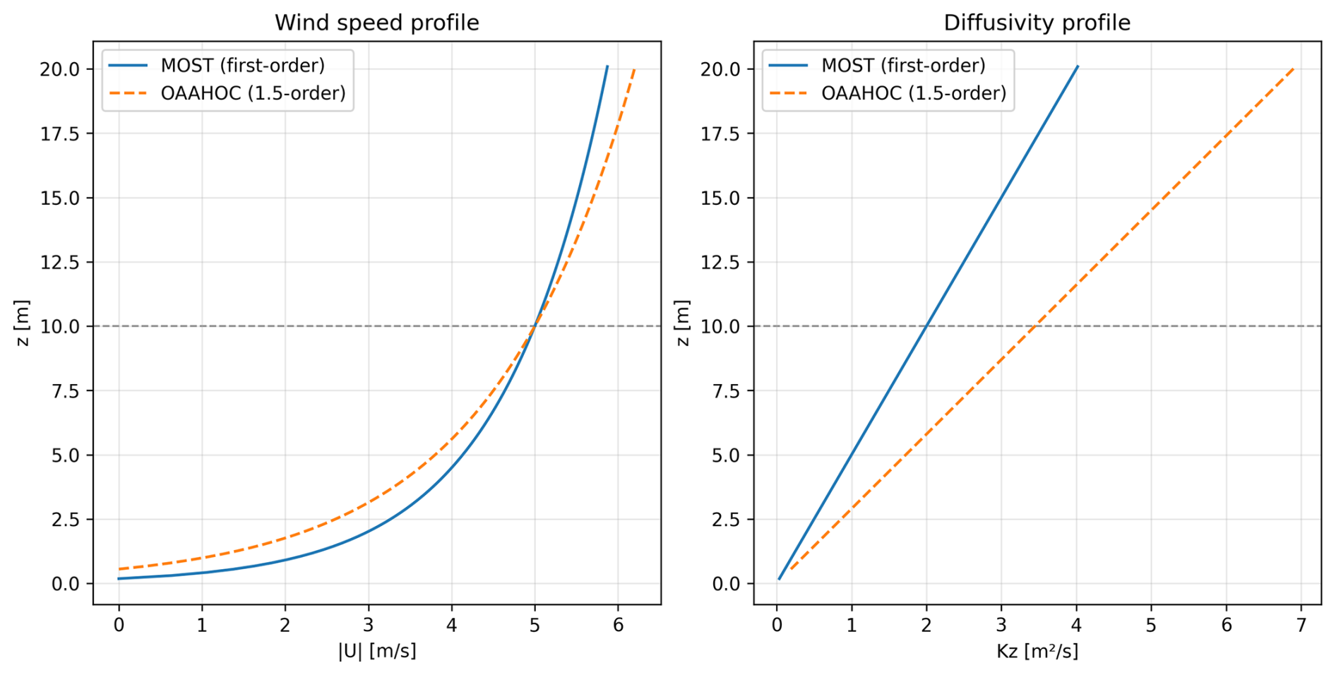
Figure 2 Demonstration of the modular turbulence-closure interface: vertical profiles of horizontal wind speed (left) and eddy diffusivity K_z (right) computed with the first-order MOST closure and the one-and-a-half-order Schumann–Lilly closure (OAAHOC; Schumann, 1991) under otherwise identical conditions. The dashed horizontal line marks the measurement height z_M.

5 Solver verification against an analytical solution with constant profiles

As shown in Eqs. (9) and (10), the steady-state advection-diffusion equation admits an analytical solution if its coefficients are constant. This fact provides a practical test case to assess the performance of the numerical method presented in the previous section. We stress that this analytical test case, together with the convergence study in Sect. 6, constitutes a verification of the numerical solver, i.e., confirming that the code correctly solves the governing equations under idealized conditions, rather than a validation of the physical footprint model under realistic atmospheric conditions, which we defer to future work (see Sect. 8).

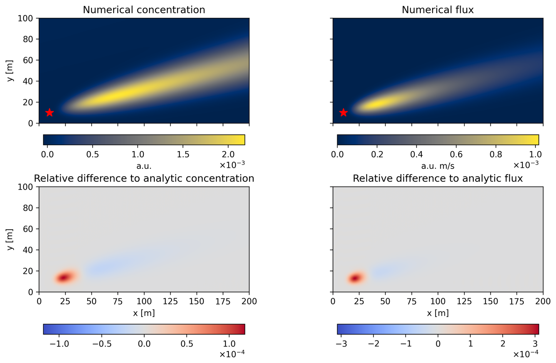
Figure 3 Dispersion experiment with unit point source at the red star. Comparison with analytical solution for constant profiles of horizontal wind and eddy diffusivities. Top row: concentration and flux at 10 m computed with the BLDFM numerical scheme. Bottom row: relative differences to the analytic solution.

Figure 3 shows results from a comparison of the numerical solution for a dispersion experiment with the analytical solution when $u,v,K_{\mathrm{h}}$ and K_z are set constant. The top two plots show the plume of the scalar Φ and its flux at z_M=10 m caused by a unit point source at the surface marked by a red star. The bottom two plots show the associated relative differences to the analytical solution as

$$\begin{array}{}\text{(34)}& {\displaystyle }{\mathrm{\Delta }}_{\mathrm{rel}}\mathrm{\Phi }={\displaystyle \frac{{\mathrm{\Phi }}_{\mathrm{numerical}}-{\mathrm{\Phi }}_{\mathrm{analytic}}}{max\left({\mathrm{\Phi }}_{\mathrm{analytic}}\right)}}.\end{array}$$

The wind in the test simulation is set to ${\mathit{u}}_{\mathrm{h}}=(\mathrm{4.0},\mathrm{1.0}{)}^T\mathrm{m}{\mathrm{s}}^{-\mathrm{1}}$ and eddy diffusivity $K_{\mathrm{h}}=K_z=\mathrm{1.6}\mathrm{m}{\mathrm{s}}^{-\mathrm{2}}$. These values are chosen to depict typical meteorological conditions in the planetary boundary layer. 512 Fourier modes and 256 vertical grid points are used for the numerical integration with the third-order method as described in Sect. 2 and Appendix A, which might be slightly excessive for usual applications but still is sufficiently fast on a modern desktop computer. Our computer runs an 11th generation Intel^®Core™ i7 processor at 2.50 GHz and has 16 GiB RAM installed. BLDFM was implemented and compiled with Python 3.13.2. On a single core, the (unparallelized) simulation took 9 s.

The results are as expected and a typical plume is generated (cf. Stockie, 2011). The comparison with the analytical solution reveals a remarkably good agreement: the maximum relative difference is less than 1 ‰. In conclusion, the numerical integrator of BLDFM demonstrates robust performance in the designed test case scenario, effectively solving the problem with high accuracy and efficiency.

6 Numerical error convergence analysis

We performed an error convergence study to verify the numerical PDE solver of BLDFM and test its scalability.

Two different tests were executed. In the ANALY experiment, the difference between the numerical and the analytical solution with constant profiles of the previous Sect. 5 was computed with increasing resolution. As the analytical plume requires constant wind and eddy diffusivity profiles, the vertical integration by the exponential integrator method is, in fact, exact and hardly challenged in the ANALY experiment. Therefore, the HI-RES experiment utilizes a high-resolution numerical solution with profiles according to MOST (cf. Sect. 4) as the reference solution. The error between the numerical solution and the reference solution was computed for various resolutions.

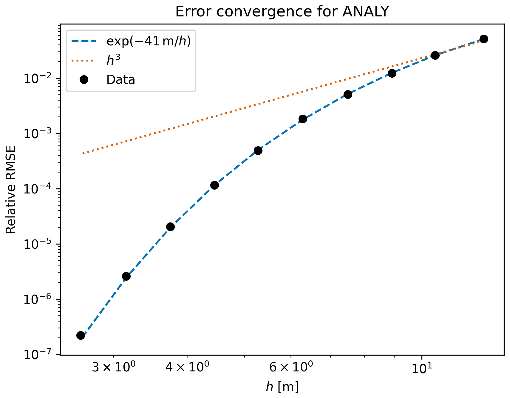
Figure 4 Relative error against resolution measured by effective grid size h from the ANALY experiment. Each black dot represents a simulation with different resolution. The dashed (blue) curve represents a best fit curve to an exponential. The dotted (orange) curve is a third-degree monomial representing third-order error convergence as an upper bound for the theoretical error. The actual error drops exponentially faster with increasing resolution that is decreasing grid size.

Vertical and horizontal resolution were varied simultaneously. The results of the ANALY experiment are shown in Fig. 4. It can be observed that the error decays exponentially with increasing resolution or decreasing effective grid size, $h=\sqrt[\mathrm{3}]{\mathit{\delta }x\mathit{\delta }y\mathit{\delta }z}$, respectively, which is typical for the Fourier method and to be expected. We quantified the error convergence by fitting the exponential curve $\propto \exp (-r/h)$ to get the exponential error convergence rate r. For the ANALY experiment, we find r=41 m indicating extremely rapid error decay. Indeed, going to even higher resolutions (not shown here), we quickly reached the limit of machine accuracy. Since we use a third-order Taylor expansion of the exponential integrator method in the vertical integration, a polynomial (third order) or mixed error convergence is to be expected in the HI-RES experiment. However, as shown in Fig. 5, the exponential curve provides a good fit, although with a slightly reduced exponential error decay rate of r=35 m such that mainly exponential error convergence seems to be at play dominating the error decay. For comparison, a third-degree monomial is additionally plotted in Figs. 4 and 5 to highlight the rapid error convergence. It should also be noted that the offset in the HI-RES curve is marginally higher in comparison to ANALY. For most practical applications of BLDFM, we conclude favorable scalability such that relatively low resolutions suffice for standard cases such as footprint calculations, rendering BLDFM a fast and accurate solver.

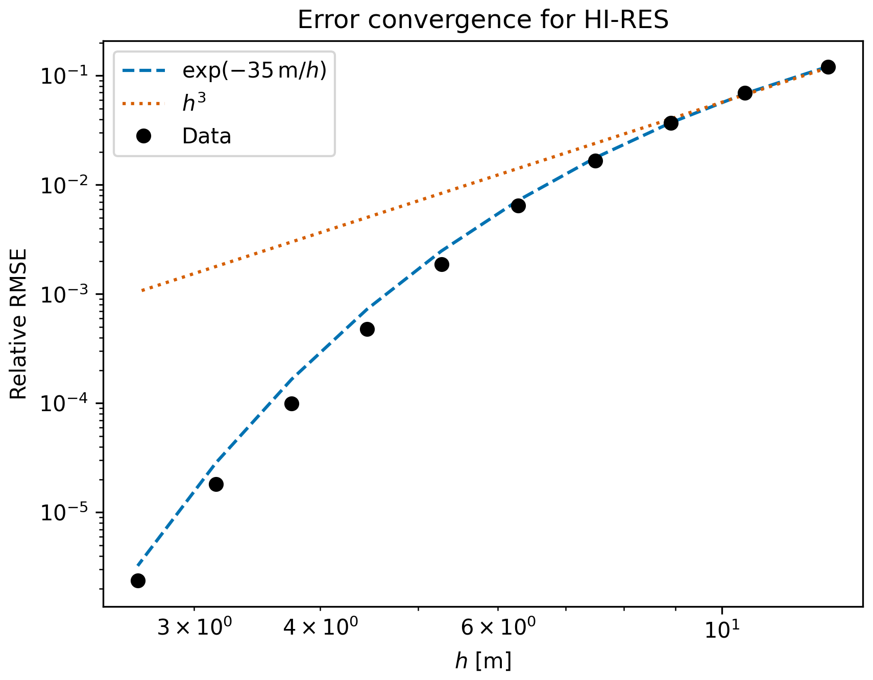
Figure 5 Relative error against resolution measured by effective grid size h from the HI-RES experiment. Each black dot represents a simulation with different resolution. The dashed (blue) curve represents a best fit curve to an exponential. The dotted (orange) curve is a third-degree monomial representing third-order error convergence as an upper bound for the theoretical error. The actual error drops exponentially faster with increasing resolution that is decreasing grid size.

Figure 6 Footprints of BLDFM, modified BLDFM-SP with slender plume approximation and the Kormann and Meixner footprint model (KM01), subject to neutral stability conditions of the atmospheric boundary layer. The red stars mark the position of the receptor (see Sect, 7.1 for more details).

7 Comparison with the Kormann and Meixner footprint model

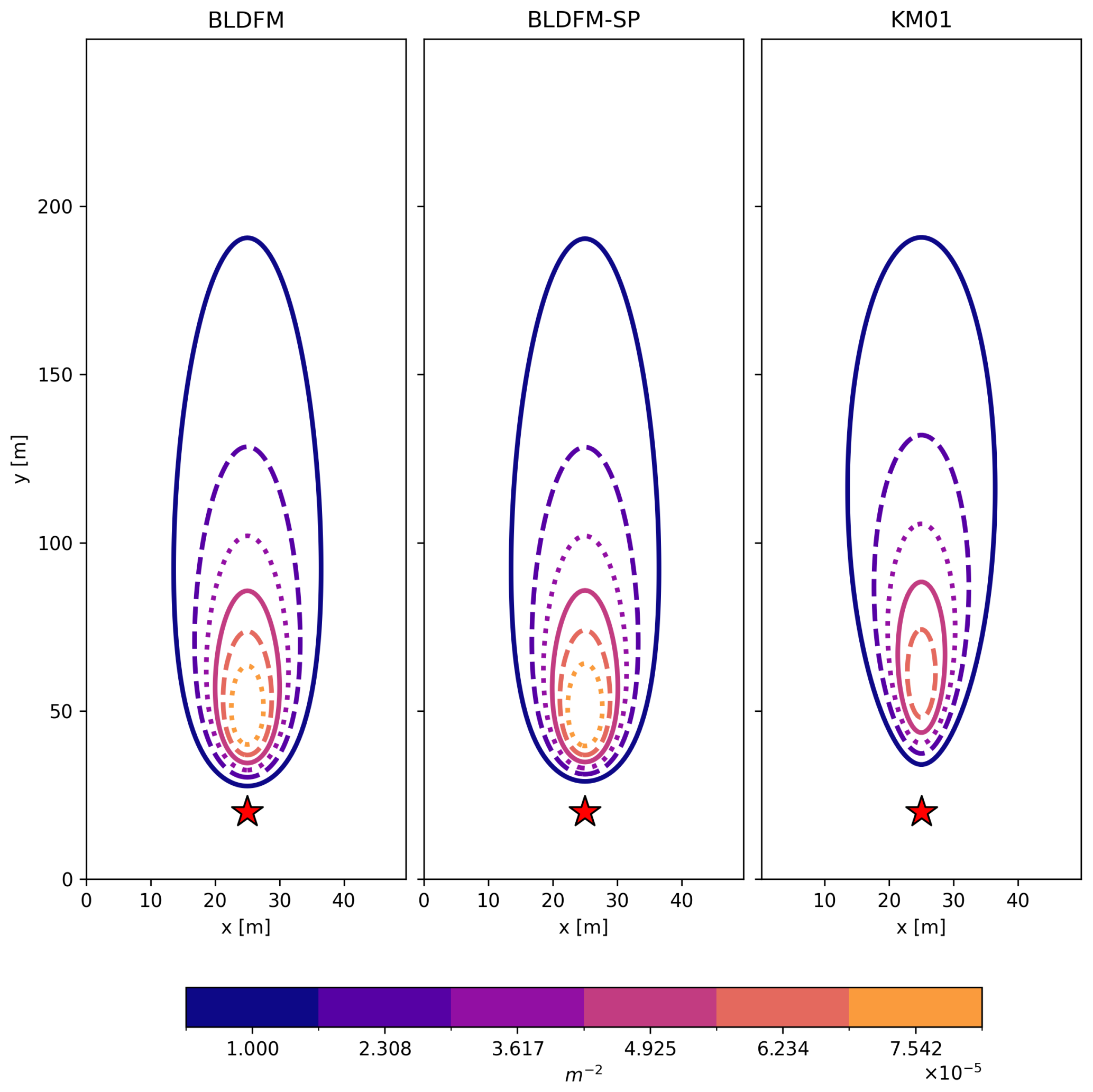
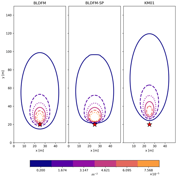
To assess BLDFM's capabilities as a flux footprint model, we ran three different test cases for various stratification scenarios of the boundary layer and compared the results with the well-established and widely used footprint model of Kormann and Meixner (2001, hereafter referred to as KM01). The KM01 model follows a diametrically opposite paradigm compared to BLDFM. In contrast to BLDFM's numerical approach, KM01 is based on an analytical closed-form solution of the steady-state advection-diffusion equation subject to two simplifications:

1. The slender plume assumption: turbulent diffusion in the streamwise direction is neglected.

2. Vertical profiles of the horizontal wind velocity and eddy diffusivity are modeled in terms of power laws. Profiles from Monin-Obukhov Similarity Theory are then approximated by the power law representation, with reported deviations of up to 15 %.

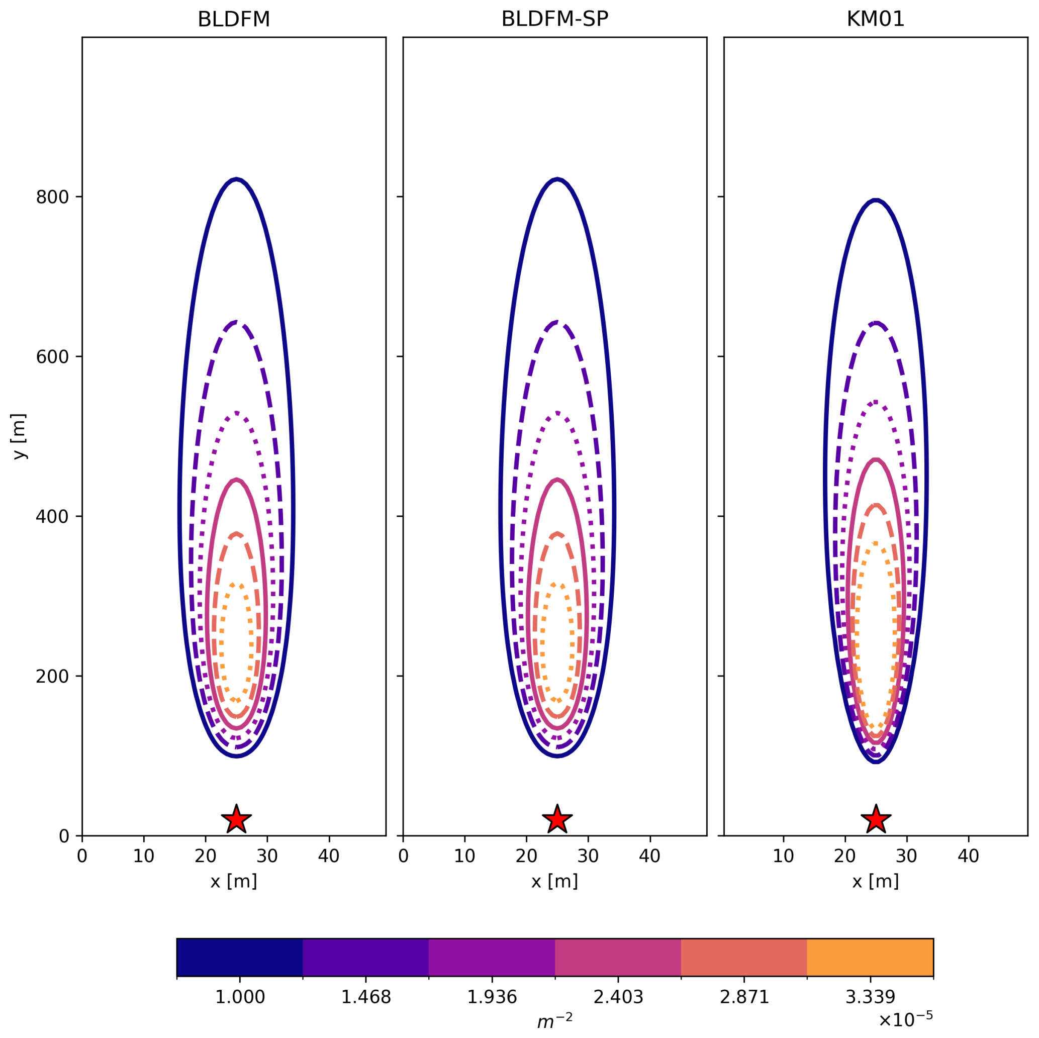
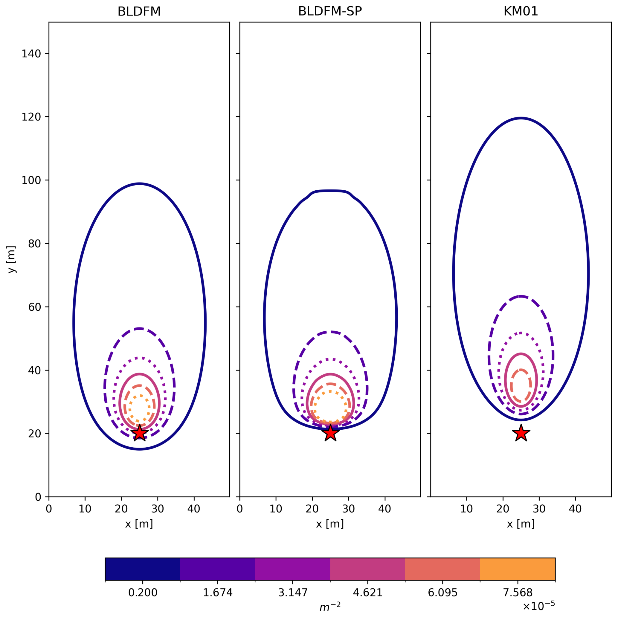
BLDFM does not require either of these two simplifications: owing to its numerical approach, it retains streamwise turbulent diffusion and uses the Monin-Obukhov profiles directly rather than approximating them with power laws. To attribute and understand the differences in the performances between BLDFM and KM01, we implemented a modified version of BLDFM constrained by the slender plume assumption, where streamwise eddy diffusion is switched off. This version is called BLDFM-SP. In all three experiments, the wind blows from the North at 5.0 m s⁻¹, a roughness length of z₀=0.5 m is assumed and the measurement point is at $(x_{\mathrm{M}},y_{\mathrm{M}}{)}^{\mathrm{T}}=(\mathrm{25.0},\mathrm{20.0}{)}^{\mathrm{T}}$ m with a height of z_M=10.0 m. The atmospheric stability is quantified by the dimensionless stability parameter $z_{\mathrm{M}}/L$ evaluated at the measurement height, where $z_{\mathrm{M}}/L=\mathrm{0}$ denotes neutral, $z_{\mathrm{M}}/L>\mathrm{0}$ stable and $z_{\mathrm{M}}/L<\mathrm{0}$ unstable stratification.

7.1 Neutrally stratified boundary layer

Figure 6 shows a comparison of the footprints from BLDFM and KM01 under neutral conditions such that the stability parameter is $z_{\mathrm{M}}/L=\mathrm{0}$. The footprints of BLDFM, BLDFM-SP and KM01 look similar. All footprints have a comparable fetch, i.e., the distance over which the wind can effectively mix or advect the scalar from its source to the receptor. There is no significant difference between BLDFM and BLDFM-SP. Upon close inspection, the shape of the KM01 footprint is slightly warped in comparison to the BLDFM footprints. This discrepancy can be attributed to the different formulations of crosswind standard deviation or dispersion σ. For BLDFM, eddy diffusion is horizontally homogeneous such that σ² scales with the distance from the receptor ξ. In the KM01 model, however, σ²∝ξ². Therefore, horizontal eddy diffusion actually increases with distance from the receptor for KM01, which implies horizontally inhomogeneous eddy diffusion. The difference in horizontal eddy diffusion between both models also explains BLDFM's peak of the footprint being marginally closer to the receptor and considerably larger in magnitude.

Figure 7 Footprints of BLDFM and the Kormann and Meixner footprint model under very stable conditions of the atmospheric boundary layer (see Sect, 7.2 for more details).

7.2 Stable boundary layer

Figure 7 shows a comparison of the footprints from BLDFM and KM01 under stable conditions. All features are the same as in the previous case, but the stability parameter is chosen to be $z_{\mathrm{M}}/L=\mathrm{1}$, i.e., very stable atmospheric conditions. Both models, BLDFM and KM01, generate similar footprints. There is no significant difference between BLDFM and BLDFM-SP. The main difference between the footprints is the fetch, which is recognizably shorter for KM01. This difference between BLDFM and KM01 may be explained by the fact that the KM01 model approximates the wind profiles with a power law. As KM01 reports deviations up to 15 % in the profiles, this explanation seems plausible. Apparently, KM01 underestimates the horizontal wind, which can be attributed to the shorter fetch. In contrast, BLDFM uses the profiles from MOST directly as input for the numerical integration.

7.3 Unstable boundary layer

Figure 8 presents a comparison of the footprints from BLDFM and KM01 under unstable conditions. The stability parameter is $z_{\mathrm{M}}/L=-\mathrm{1}$ and, hence, the atmospheric conditions are very unstable. Here, the differences between BLDFM, BLDFM-SP and KM01 are most pronounced. We notice in particular a significant discrepancy between BLDFM and BLDFM-SP. The slender plume assumption leads to a shorter fetch of the footprint. Furthermore, BLDFM's footprint extends into the lee of the receptor due to the enhanced vertical mixing, which contrasts with BLDFM-SP, where no material can be mixed against the mean wind as streamwise mixing is suppressed. The same can be observed for KM01, where the edge of the footprint is even farther away from the measurement point than BLDFM-SP. In contrast to BLDFM-SP, however, KM01's fetch is longer than for BLDFM. The difference, therefore, cannot be explained by the slender plume assumption and may be attributed to the approximated wind profiles of KM01. Especially for very unstable atmospheric conditions, the wind has a strongly sheared profile, which is challenging to approximate with a power law. It is likely that KM01 overestimates the horizontal wind speed to compensate for the shortening effect of the slender plume assumption, which would explain the prolonged fetch.

Figure 8 Footprints of BLDFM and the Kormann and Meixner footprint model under very unstable conditions of the atmospheric boundary layer (see Sect. 7.3 for more details).

8 Conclusions

This paper presents a novel atmospheric dispersion and footprint model called the Boundary Layer Dispersion and Footprint Model (BLDFM) for applications on the microscale in the atmospheric boundary layer for various turbulent regimes dependent on atmospheric stability. The model solves the three-dimensional steady-state advection-diffusion equation in Eulerian form numerically. The Fourier method was utilized to transform the transport problem into a family of second-order ordinary differential equations posing an eigenvalue problem. In combination with flux boundary conditions, the problem was converted into a boundary value problem, which can be efficiently solved with the linear shooting method. This numerical formulation allows for usage of the Fast Fourier Transform in combination with the Exponential Integrator Method, resulting in a computationally fast and robust algorithm.

Vertical profiles of mean wind and eddy diffusivity were computed by Monin-Obukhov Similarity Theory, taking the stability of the boundary layer into account. Beyond the first-order MOST closure, we also implemented and demonstrated a one-and-a-half-order closure (Sect. 4.1), illustrating the modularity of the framework. Interfacing higher-order (e.g. second-order) closure schemes are left for future work. Notice that vertical wind and diffusivity profiles are represented directly on the grid with user-defined precision, which stands in stark contrast to (semi-)analytical footprint models where the profiles need to be fitted to auxiliary functions for which closed-form analytical expressions can be derived. The grid representation is also designed to accept measured or simulated profiles directly, e.g., from Large-Eddy Simulations, a capability we plan to validate and use in future work.

The numerical solver of BLDFM has been verified against a special analytical solution. Under typical atmospheric conditions and moderately high resolution, the relative difference between numerical and analytical solutions is less than 1 ‰. Numerical convergence tests reveal exponential error decay with substantially high decay rates, suggesting favorable scalability. Comparisons with the Kormann and Meixner footprint model (KM01) for neutral, very stable and very unstable conditions showed general agreement. However, discrepancies in the fetch of the footprints were identified. We associated those differences with KM01's neglect of turbulent mixing in the stream direction and the approximation of the vertical profiles with power laws. Those are necessary assumptions in analytical footprint models to obtain closed-form expressions. However, BLDFM takes the full three-dimensional turbulent mixing into account and uses the logarithmic profiles according to Monin-Obukhov similarity theory. In a future publication, it is planned to validate BLDFM against data from tracer release experiments.

Appendix A: Derivation of the exponential integrator

In Sect. 2 we introduced the Exponential Integrator Method to solve the initial value problem arising from the linear shooting method. We discretize the vertical axis by increments $z^{\left(n\right)}=z_{\mathrm{0}}+n\mathit{\delta }z$ such that for any function $f={\mathit{u}}_{\mathrm{h}},K_{\mathrm{h}},K_z,\mathrm{\dots }$ we write f(z⁽ⁿ⁾)=f⁽ⁿ⁾. Then, according to Hochbruck and Ostermann (2010), we may derive the following iteration scheme in terms of the exponential integrator method,

$$\begin{array}{ll}\text{(A1)}& {\displaystyle }{\mathit{\eta }}^{\left(n\right)}& {\displaystyle }=-K_{\mathrm{h}}^{\left(n\right)}|\mathit{\mu }{|}^{\mathrm{2}}-\mathrm{i}\mathit{\mu }\cdot {\mathit{u}}_{\mathrm{h}}^{\left(n\right)},\text{(A2)}& {\displaystyle }{\mathit{\lambda }}^{\left(n\right)}& {\displaystyle }=\sqrt{{\mathit{\eta }}^{\left(n\right)}/K_z^{\left(n\right)}},{\displaystyle }{\mathit{\phi }}^{(n+\mathrm{1})}& {\displaystyle }=\cos \left({\mathit{\lambda }}^{\left(n\right)}\mathit{\delta }z\right){\mathit{\phi }}^{\left(n\right)}-{\displaystyle \frac{\mathrm{1}}{{\mathit{\lambda }}^{\left(n\right)}{K}_z^{\left(n\right)}}}\\ \text{(A3)}& {\displaystyle }& {\displaystyle }\sin \left({\mathit{\lambda }}^{\left(n\right)}\mathit{\delta }z\right)q^{\left(n\right)},\text{(A4)}& {\displaystyle }{q}^{(n+\mathrm{1})}& {\displaystyle }={\displaystyle \frac{{\mathit{\eta }}^{\left(n\right)}}{{\mathit{\lambda }}^{\left(n\right)}}}\sin \left({\mathit{\lambda }}^{\left(n\right)}\mathit{\delta }z\right){\mathit{\phi }}^{\left(n\right)}+\cos \left({\mathit{\lambda }}^{\left(n\right)}\mathit{\delta }z\right)q^{\left(n\right)}.\end{array}$$

Note that this solution is exact given that all coefficients are constant in the interval $z^{\left(n\right)}<z<z^{(n+\mathrm{1})}$. This key property, which holds for linear equations, sets the Exponential Integrator Method apart from other numerical solvers. Since the atmospheric transport equations are indeed linear, it is hence the favored choice for BLDFM. A less accurate but computationally faster algorithm emerges when taking the third-order Taylor approximation of the exponential integrator, which can be achieved by expanding the cosine and sine as

$$\begin{array}{}\text{(A5)}& {\displaystyle }\cos \left(x\right)& {\displaystyle }=\mathrm{1}-{\displaystyle \frac{\mathrm{1}}{\mathrm{2}}}{x}^{\mathrm{2}}+\mathcal{O}(\Vert x{\Vert }^{\mathrm{4}}),\text{(A6)}& {\displaystyle }\sin \left(x\right)& {\displaystyle }=x-{\displaystyle \frac{\mathrm{1}}{\mathrm{6}}}{x}^{\mathrm{3}}+\mathcal{O}(\Vert x{\Vert }^{\mathrm{4}}).\end{array}$$

Since the iteration scheme Eqs. (A1)–(A4) is carried out for each tuple (n,m) independently, a significant acceleration of its implementation is achieved when executing it in parallel.

Appendix B: Stretched vertical coordinates

In most use cases of BLDFM, the scalar or flux is evaluated at a certain measurement height z_M. To minimize numerical errors stemming from the upper boundary, the vertical integration (cf. Appendix A) is carried out until z_T, which is ideally very far away from z_M. Optimally, z_T is greater than the blending height, i.e. the height above the surface at which the influence of the heterogeneous surface on a given quantity becomes insignificant. Since the latter depends on many external factors, we set z_T=2z_M by default. As the signal from the surface is blended with increasing height by mixing, a coarser resolution of the vertical grid may suffice at higher levels to obtain accurate solutions. Therefore, we utilize a stretched vertical coordinate ζ, which allows for fewer vertical grid cells and hence faster computation, as follows,

$$\begin{array}{}\text{(B1)}& {\displaystyle }z\left(\mathit{\zeta }\right)& {\displaystyle }=H\ln \left({\displaystyle \frac{b}{a-\mathit{\zeta }}}\right)\iff \mathit{\zeta }\left(z\right)=a-b\exp \left(-{\displaystyle \frac{z}{H}}\right),\text{(B2)}& {\displaystyle }a& {\displaystyle }=b\exp \left(-{\displaystyle \frac{z_{\mathrm{0}}}{H}}\right),\text{(B3)}& {\displaystyle }b& {\displaystyle }={\displaystyle \frac{z_{\mathrm{M}}}{\exp (-z_{\mathrm{0}}/H)-\exp (-z_{\mathrm{M}}/H)}},\end{array}$$

where H determines the magnitude of stretching. It was found that H=2z_M gives a good compromise between accuracy and efficiency. The parameters a and b were chosen such that ζ(z_M)=z_M and ζ(z₀)=0, which guarantees that z(ζ_N)=z_M when we discretize ζ_n=n δζ with $\mathit{\delta }\mathit{\zeta }=z_{\mathrm{M}}/N$.