Development of the TCWA2 bulk cloud microphysics scheme and its integration with a dual-polarization radar operator for forecasting applications

This study presents the development and evaluation of TCWA2, a double-moment bulk cloud microphysics scheme designed for weather forecasting that incorporates radar observations at the Taiwan Central Weather Administration. By simplifying the triple-moment NTU microphysics scheme, TCWA2 retains a gamma-type particle size distribution with variable spectral parameters, diagnoses hydrometeor-associated physical properties, revises number sinks due to evaporation loss, and implements theoretically based fall-speed formulations that account for particle density and aspect ratio. To connect bulk microphysics parameterizations with radar-based diagnostics, TCWA2 is coupled with a customized bulk dual-polarization radar operator derived from offline bin-based scattering calculations under the Rayleigh approximation. This integrated microphysics–radar system provides an internally consistent representation linking particle-size distribution characteristics, hydrometeor morphology, sedimentation processes, and bulk radar observables.

The intrinsic behavior of TCWA2 is first examined through two-dimensional idealized squall-line simulations in the Weather Research and Forecasting (WRF) model, which produce physically interpretable microphysical structures and coherent polarimetric radar signatures. The scheme is further demonstrated through a proof-of-concept real-case simulation of an afternoon convective event using the Model for Prediction Across Scales (MPAS), with comparisons against observed dual-polarization radar measurements. The joint distributions of radar reflectivity and polarimetric variables show encouraging agreement with observations, with pattern correlations exceeding 0.9 across three altitude layers. These results suggest that TCWA2 can capture key radar-signature characteristics associated with dominant hydrometeor populations and support its potential for future radar-based forecasting applications, while further refinement of ice-phase parameterizations, particle-orientation assumptions, and radar-viewing geometry remains necessary.

1 Introduction

Cloud microphysical processes are vital for the formation, growth, and dissipation of clouds, as well as for the sedimentation of hydrometeors, exerting a strong impact on atmospheric thermodynamics and surface precipitation across various scales. In numerical weather prediction (NWP) models, these processes are typically represented by bulk microphysics parameterization (BMP) schemes, which approximate particle size distributions (PSDs) and phase changes among hydrometeor types using analytical formulas (e.g., Lin et al., 1983; Rutledge and Hobbs, 1983; Tao and Simpson, 1993). Over the decades, BMPs have evolved from basic single-moment schemes predicting mass mixing ratios to more advanced double- and triple-moment schemes that explicitly forecast additional moments such as number concentration, surface area, and radar reflectivity factor (e.g., Milbrandt and Yau, 2005b; Chen and Tsai, 2016, hereinafter CT16; Morrison et al., 2025). In addition to size-spectrum representations, recent developments include associated variables such as particle shape, density, and liquid fraction in ice particles to better depict hydrometeor morphology (e.g., Harrington et al., 2013a; Morrison and Milbrandt, 2015; Jensen et al., 2017; Tsai and Chen, 2020, hereinafter TC20; Milbrandt et al., 2025). Despite these advancements, substantial uncertainties persist in representing the inherent variability of cloud microphysical properties (Fan et al., 2017), as well as those arising from cloud dynamics, turbulence, and unresolved cumulus thermal processes in km-scale models (Hernandez-Deckers et al., 2022). These limitations continue to challenge NWP models' ability to accurately simulate storm structures and precipitation. Such issues emphasize the need for a physically consistent modeling framework that can directly connect microphysical variability with observational constraints.

Radar observations have become indispensable tools for assessing BMPs' performance and diagnosing cloud microphysical structures and precipitation mechanisms (Bringi and Chandrasekar, 2001; Ryzhkov and Zrnić, 2019). The Central Weather Administration (CWA) operates a dual-polarization radar network over Taiwan, but effectively integrating these high-resolution observations into NWP models remains a challenge. Compared to traditional single-polarization radars, dual-polarization (dual-polarimetric) systems provide additional insights on hydrometeor size, shape, and phase through observables such as horizontal radar reflectivity (D_BZ), differential reflectivity (Z_DR), and specific differential phase (K_DP) (Ryzhkov et al., 2011; Kumjian, 2013). Many studies (e.g., Kumjian and Ryzhkov, 2008; Kumjian and Prat, 2014; Johnson et al., 2016) have examined the connections between hydrometeor properties and dual-polarimetric radar signatures to better understand cloud microphysics. However, a significant gap persists between model-predicted microphysics and radar forward operators. Most current BMPs do not explicitly predict or output the key physical quantities needed for accurate radar forward calculations, such as full PSD parameters, particle aspect ratios, or apparent density. For instance, the spectral shape parameter in PSD is critical for determining microphysical growth rates (cf. CT16) and terminal velocities (Milbrandt and Yau, 2005a), yet its influence is often overlooked or oversimplified in microphysical models and radar operators. Therefore, radar operators frequently rely on external assumptions or empirical lookup tables that are not directly constrained by the microphysics scheme itself (Pfeifer et al., 2008; Jung et al., 2008; Wolfensberger and Berne, 2018; Matsui et al., 2019; Zhang et al., 2021), which can lead to physical inconsistencies and complicate the interpretation of modeled radar signatures (Putnam et al., 2014). Furthermore, hydrometeor properties inferred from radar can greatly affect microphysical processes, including collision, sedimentation, and deposition, underscoring the importance of explicitly accounting for particle morphology within BMPs.

Although some recent BMPs have begun to introduce additional hydrometeor characteristics to improve the physical representation, most remain computationally prohibitive for real-time NWP applications. An example is the National Taiwan University (NTU) three-moment bulk microphysics scheme (CT16; TC20), which predicts the bulk shape and density of solid-phase hydrometeors using a three-moment closure approach. However, the full NTU formulation involves numerous prognostic moments and complex process treatments, making it impractical for current operational forecasting applications. To address these limitations, this study develops a simplified version of the NTU scheme, hereafter called TCWA2 (Taiwan Central Weather Administration 2-moment), which retains the core framework and reduces computational costs by replacing prognostic moments with constrained diagnostic parameterizations. The TCWA2 scheme emulates the NTU scheme by diagnosing the spectral shape parameter of PSD and other bulk properties needed for dual-polarization radar calculations, enabling direct coupling with a radar forward operator. This integration allows the model to predict radar observables in real time and provides a unified framework for radar-based model evaluation. TCWA2 has been implemented in both the Weather Research and Forecasting (WRF) version 4.4.2 (Skamarock et al., 2019) and the Model for Prediction Across Scales (MPAS) version 8.2.2 (Skamarock et al., 2012, 2018), developed by the National Center for Atmospheric Research (NCAR).

The rest of this paper is organized as follows. Section 2 outlines the formulation and methodology of the TCWA2 scheme, including the diagnostic PSD parameters, associated hydrometeor properties, and dual-polarization bulk radar operator. Section 3 presents a two-dimensional idealized simulation using the WRF model to evaluate the scheme's fundamental behavior and internal consistency. Section 4 applies the TCWA2–radar coupled system to a proof-of-concept real convective case from the TAHOPE (Taiwan-Area Heavy rain Observation and Prediction Experiment) field campaign on 24 June 2022, simulated with the MPAS model and compared against dual-polarimetric radar observations. Finally, Sect. 5 summarizes the results, remaining limitations, and potential applications.

2 Methodology

The classification of hydrometeor types in the TCWA2 scheme aligns with that of the NTU microphysics parameterization. Liquid-phase species include cloud droplets (CD) and raindrops (RD), whereas ice-phase species consist of pristine ice (PI), snow aggregates (SA), and rimed ice (RI). These three ice categories are differentiated by their main formation processes: deposition for PI, aggregation for SA, and riming for RI. The hailstone category is merged into RI, and the distinction between graupel and hail is based on the Schumann–Ludlam limit (SLL; Ziegler, 1985). In addition, the explicit tracking of aerosol groups (condensation nuclei and ice nuclei) and their activation using a semi-Lagrangian technique is replaced by a predicted supersaturation approach (Chen, 1994; Morrison and Milbrandt, 2015). Prescribed initial activation diameters are 3 µm for cloud droplets (Lim and Hong, 2010) and 6 µm for ice crystals (CT16; D_i0). As a result, the total number of prognostic variables decreases to eleven in a fully double-moment, five-category scheme – a significant contrast to the twenty-seven variables required by the triple-moment, six-category NTU configuration. The following subsections illustrate how the prognostic second-order, shape, and volume moments in the NTU scheme are replaced by diagnostic parameterizations in TCWA2, and integrated with an embedded bulk dual-polarization radar operator.

2.1 Particle size distribution

BMPs commonly represent hydrometeor PSD by applying a three-parameter gamma distribution in the form (Ulbrich, 1983):

$$\begin{array}{}\text{(1)}& n\left(D\right)=N_{\mathrm{0}}{D}^{\mathit{\alpha }}{e}^{-\mathit{\lambda }D},\end{array}$$

where N₀, α, and λ denote the intercept, spectral shape, and slope parameters, respectively. The kth moment of the PSD defined in Eq. (1) is given by

$$\begin{array}{}\text{(2)}& \begin{array}{rl}{M}_k& =\int D^{k}n\left(D\right)\mathrm{d}D=N_{\mathrm{0}}\int D^{k+\mathit{\alpha }}\exp \left(-\mathit{\lambda }D\right)\mathrm{d}D\\ & ={\displaystyle \frac{N_{\mathrm{0}}\mathrm{\Gamma }(k+\mathit{\alpha }+\mathrm{1})}{{\mathit{\lambda }}^{k+\mathit{\alpha }+\mathrm{1}}}},\end{array}\end{array}$$

where k is the order of the moment, and Γ is the Euler gamma function. The spectral shape α controls the spectral width of the PSD and greatly influences microphysical conversion rates. In most double-moment schemes, α is either fixed at a constant value (e.g., Morrison et al., 2009; Lim and Hong, 2010) or modeled as an empirical function of particle mean size related to a single growth process (e.g., Milbrandt and Yau, 2005a), implying a uniform spectral response across different microphysical regimes. However, Morrison et al. (2025) showed that PSDs exhibit distinct evolutionary behaviors when driven by different microphysical processes, as revealed by a triple-moment closure framework. Similarly, the physically based triple-moment NTU scheme predicts the zeroth- (k=0), second- (k=2), and third-order (k=3) moments, allowing α to change freely over time. The temporal evolution of these prognostic moments is driven by three key microphysical processes: initiation, vapor diffusion, and collision. According to TC20 simulations (their Fig. 8), large α values generally correspond to small ice particles with high number concentrations at higher levels, whereas small α values are linked to large aggregated or rimed ice above the melting layer or within convective cores. As a result, α is modulated not only by variations in particle size (volume) but also by other moments, specifically number concentration and a third moment (e.g., M₂ or M₆). This multi-moment dependency is reflected in the sensitivity of α to the intermediate parameter q, which involves all three moments:

$$\begin{array}{}\text{(3a)}& \mathit{\alpha }={\displaystyle \frac{\mathrm{6}-\mathrm{3}q+\sqrt{q(q+\mathrm{8})}}{\mathrm{2}(q-\mathrm{1})}},\end{array}$$

where $q\equiv \frac{M_{\mathrm{0}}{M}_{\mathrm{3}}^{\mathrm{2}}}{M_{\mathrm{2}}^{\mathrm{3}}}$ for triple moment schemes tracking M₀, M₂, and M₃ (TC20). In general, vapor diffusion increases α, leading to a narrower PSD (cf. CT16), whereas collision growth decreases α and broadens the PSD. These contrasting behaviors reflect the fundamental differences in how growth processes affect different moments. For example, the condensation process increases M₂ linearly, increases M₃ sub-linearly, but does not alter M₀. On the other hand, the collision-coalescence process is mass conservative but reduces M₀ and M₂. Thus, α should respond differently to different processes according to Eq. (3a).

Diagnostic formulas of α in TCWA2 were derived by analyzing NTU scheme simulations, utilizing calculated moments or their proxies such as mean particle size as predictors for both the accretional and diffusional regimes.

$$\begin{array}{}\text{(3b)}& {\mathit{\alpha }}_x={\displaystyle \frac{a+b\ln N_x+c\ln N_x^{\mathrm{2}}+d\ln R_x}{\mathrm{1}+e\ln N_x+f\ln R_x}}\end{array}$$

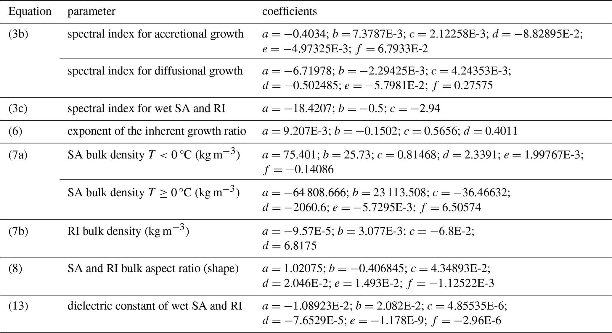
where $x\in \left(\mathrm{r},\mathrm{i},\mathrm{s},\mathrm{g}\right)$ denotes the hydrometeor category, and the empirical coefficients a through f are listed in Table 1. The mean-volume radius $R_x={\left(\frac{\mathrm{3}{Q}_x}{\mathrm{4}\mathit{\pi }{N}_x{\mathit{\rho }}_x}\right)}^{\mathrm{1}/\mathrm{3}}$ in meters is derived from the mass mixing ratio (Q_x), number concentration ($N_x=M_{\mathrm{0},x}$), and bulk density (ρ_x). The accretional mode is activated when cloud water coexists with a hydrometeor x, representing conditions under which collision or riming dominates the PSD evolution. In the absence of cloud water, diffusional growth or sublimation governs particle growth, and the diffusional mode is therefore applied. Figure 1a and b illustrates the dependence of α (ranging from 0 to 30) on number concentration and mean-volume radius for accretional and diffusional growth, respectively. In the accretional regime, α decreases with increasing size and decreasing N_x, indicating PSD broadening due to collisions. In contrast, diffusional growth results in larger α values for larger sizes and lower N_x, reflecting narrower spectra.

For wet SA and RI in the melting regime, the energy budget is governed by the combined effects of conductive heating and latent heat from freezing and evaporation. The concurrent influence of accretional and diffusional processes creates a mixed and spatially variable distribution of α within the melting layer in the TC20 simulations. Small particles that melt quickly and shrink show sudden spectral narrowing (large α), while larger partially melted ice particles keep smaller α values as they continue to gather liquid drops, contributing to the formation of the radar bright band. To capture this rapid transition between these two contrasting behaviors, TCWA2 employs an exponential diagnostic relation:

$$\begin{array}{}\text{(3c)}& {\mathit{\alpha }}_x\left(\ge \mathrm{0}\mathit{°}\mathrm{C}\right)=\exp \left(a+b\ln N_x+c\ln R_x\right)\end{array}$$

where $x\in \left(\mathrm{s},\mathrm{g}\right)$. As shown in Fig. 1c, α strongly depends on particle size and quickly decreases from large values toward zero as particles approach the millimeter scale. The melting of wet SA and RI is a major source of large raindrops and is closely linked to strong radar reflectivity. However, this spectral feature, with the rapid α transition, cannot be directly mapped onto the raindrop PSD in a double-moment BMP because there is no third moment (e.g., M₂) memory during hydrometeor conversion. To partially account for this unresolved PSD transition during intense precipitation, TCWA2 introduces an empirical adjustment activated when $R_{\mathrm{r}}^{\mathrm{6}}{N}_{\mathrm{r}}\ge {\mathrm{10}}^{-\mathrm{16}}$ m⁶ kg⁻¹, corresponding to about 40 dBZ radar reflectivity (in mm⁶ m⁻³). When the raindrop number concentration, N_r, exceeds a tuning threshold of 3.8 × 10³ kg⁻¹ (roughly a mean radius of 0.55 mm), α_r is set to its maximum (30), consistent with the high-α regime for small sizes shown in Fig. 1c. Otherwise, α_r is halved to enhance raindrop deformation effects associated with broader spectra at larger sizes. This adjustment activates only during intense rainfall and does not alter the prognostic evolution of hydrometeor mass or number. Instead, it enhances PSD flexibility, enabling the model to reproduce large Z_DR and K_DP signals simultaneously under high-reflectivity conditions.

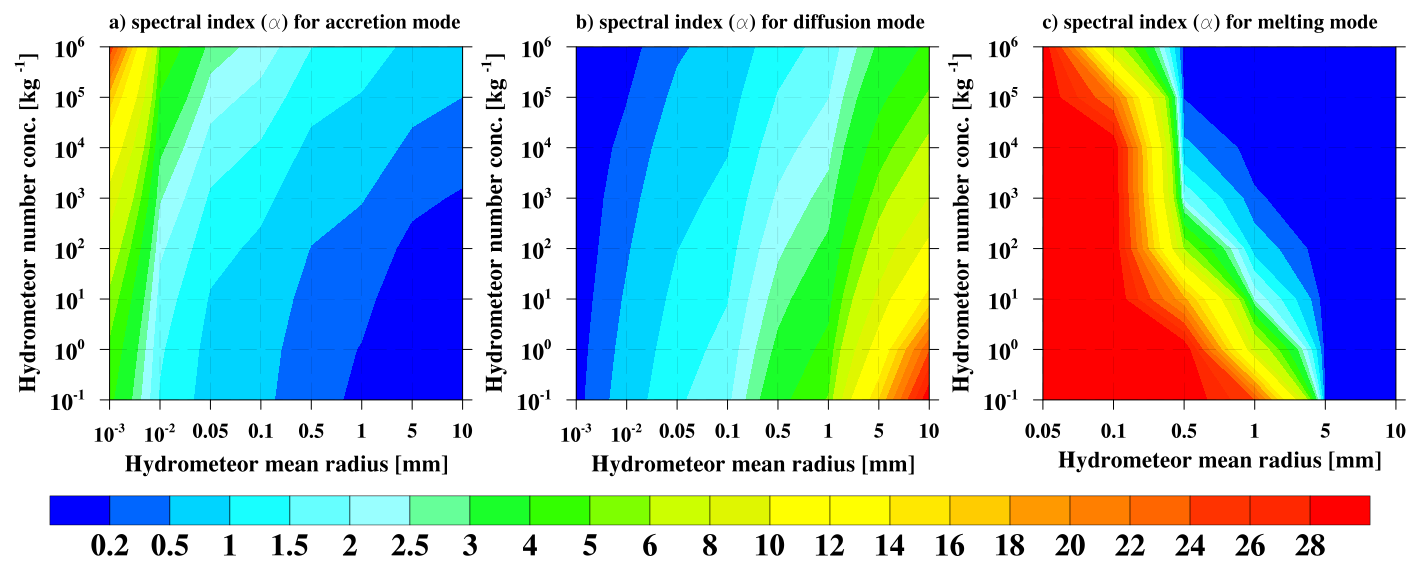
Figure 1 Spectral shape α as a function of the hydrometeor mean radius (mm) and number concentration (kg⁻¹) for accretion (left), diffusion (middle), and melting (right) modes.

Although these empirical formulations do not explicitly address process-specific forcing on the PSD, they enable TCWA2 to capture the primary physical modes of α variability without the computational cost of predicting the second-order moment (M₂). Using the diagnosed α_x and bulk density ρ_x, the remaining PSD parameters, slope λ_x and intercept N_0,x, are obtained as

$$\begin{array}{}\text{(4)}& {\displaystyle }{\mathit{\lambda }}_x={\left[{\displaystyle \frac{M_{\mathrm{0},x}\mathrm{\Gamma }\left({\mathit{\alpha }}_x+\mathrm{4}\right)}{M_{\mathrm{3},x}\mathrm{\Gamma }\left({\mathit{\alpha }}_x+\mathrm{1}\right)}}\right]}^{\mathrm{1}/\mathrm{3}}={\left[{\displaystyle \frac{\mathit{\pi }{\mathit{\rho }}_x{N}_x\mathrm{\Gamma }\left({\mathit{\alpha }}_x+\mathrm{4}\right)}{\mathrm{6}{Q}_x\mathrm{\Gamma }\left({\mathit{\alpha }}_x+\mathrm{1}\right)}}\right]}^{\mathrm{1}/\mathrm{3}},\text{(5)}& {\displaystyle }{N}_{\mathrm{0},x}={\displaystyle \frac{M_{\mathrm{0},x}{\mathit{\lambda }}_x^{{\mathit{\alpha }}_x+\mathrm{1}}}{\mathrm{\Gamma }({\mathit{\alpha }}_x+\mathrm{1})}}={\displaystyle \frac{N_x{\mathit{\lambda }}_x^{{\mathit{\alpha }}_x+\mathrm{1}}}{\mathrm{\Gamma }({\mathit{\alpha }}_x+\mathrm{1})}}.\end{array}$$

2.2 Associated physical properties

Hydrometeor properties greatly influence microphysical processes, yet developing reliable parameterizations of ice-particle shape and density remains difficult. Thus, traditional BMPs usually treat ice particles as spheres with fixed, prescribed densities (e.g., Morrison et al., 2009; Lim and Hong, 2010), and several BMPs since 2008 (e.g., Thompson et al., 2008; Milbrandt et al., 2010) have incorporated specific mass-dimension relations with exponents smaller than 3 to represent nonspherical snow structures. In contrast, the NTU scheme predicts both particle shape and density (by tracking both volume and mass) to explicitly track ice growth history. For instance, the aspect ratio of PI follows the adaptive growth habit parameterization of Chen and Lamb (1994a) and CT16. The properties of dry SA are mainly determined by the aggregation geometry among solid-phase hydrometeors (PI and SA), while the apparent density of RI is controlled by riming growth involving CD and RD. For wet SA and RI, partial melting is diagnosed from the energy budget associated with phase change. The melted fraction is calculated from the latent heat needed to melt the ice to the freezing point, and this fraction is then used to interpolate linearly between crystal properties (shape and density) and those of liquid water.

In TCWA2, the parameterization of the RD shape follows Khvorostyanov and Curry (2002), and the liquid water density ρ_w is fixed at 1000 kg m⁻³. For PI, TC20 simulations indicate that particle shape varies strongly with temperature due to the alternating dominance of columnar and planar habits, as governed by the inherent growth ratio Γ(T) within the mixed-phase regime (−40 °C $\le T\le$ 0 °C). The PI aspect ratio is expressed as ${\mathit{\varphi }}_{\mathrm{i}}\equiv {\left(\frac{D_{\mathrm{i}}}{D_{\mathrm{i}\mathrm{0}}}\right)}^{\mathrm{3}\left({\mathit{\beta }}_{\mathrm{i}}-\mathrm{1}\right)/\left({\mathit{\beta }}_{\mathrm{i}}+\mathrm{2}\right)}$, where D_i is the particle diameter and β_i is an ice adaptive growth ratio. In TCWA2, the bulk β_i is approximated as a power-law function of Γ(T), with an exponent R_t that decreases from unity (highly aspherical) at initiation to near zero (quasi-spherical) as particles approach millimeter size, expressed as follows:

$$\begin{array}{}\text{(6)}& R_t=a\ln D_{\mathrm{i}}^{\mathrm{3}}+b\ln D_{\mathrm{i}}^{\mathrm{2}}+c\ln D_{\mathrm{i}}+d\le \mathrm{1},\end{array}$$

where D_i denotes the bulk mean diameter in microns. This formulation captures the primary habit transitions between columnar and planar crystals imposed by Γ(T), while implicitly accounting for the observed reduction in intrinsic particle asphericity with increasing size (cf. CT16). The ice deposition density is retained from the NTU scheme, preserving its dependence on ice supersaturation and temperature to represent secondary growth habits (Chen and Lamb, 1994a).

For SA, data from TC20 (their Fig. 13a, c) show that bulk apparent density may fall below 300 kg m⁻³ and the aspect ratio approaches approximately 0.6 as particle size increases through aggregation, indicating a strong link between size and morphology. However, bulk density is required to derive the mean-volume radius and PSD slope parameter, so a direct size-density formulation is not practical. Instead, TCWA2 adopts an indirect diagnostic method where SA bulk density is obtained from mass concentration and air temperature via a mapped diameter from Tsai et al. (2026). The SA bulk density ρ_s is expressed as

$$\begin{array}{}\text{(7a)}& \begin{array}{rl}{\mathit{\rho }}_{\mathrm{s}}& =\exp \left(a+b\ln T_K+c\ln Q_{\mathrm{s}}+d\ln T_K^{\mathrm{2}}\right.\\ & \left.+e\ln Q_{\mathrm{s}}^{\mathrm{2}}+f\ln T_K\ln Q_{\mathrm{s}}\right),\end{array}\end{array}$$

which yields a decrease in density from approximately 400 to 100 kg m⁻³ as Q_s and T_K increases above the freezing level, while rapidly transitioning to higher densities below the melting layer as temperature rises (Fig. 2a). For RI, the bulk density ρ_g is assumed to increase monotonically with mass content from 400 kg m⁻³ and incorporates melting effects through an extrapolated melting mass fraction.

$$\begin{array}{}\text{(7b)}& \begin{array}{rl}{\mathit{\rho }}_{\mathrm{g}}& ={\mathit{\rho }}_{\mathrm{w}}{f}_{\mathrm{mw}}+(\mathrm{1}-f_{\mathrm{mw}})max\left[\mathrm{400},\exp \left(a\ln Q_{\mathrm{g}}^{\mathrm{3}}\right.\right.\\ & \left.\left.+b\ln Q_{\mathrm{g}}^{\mathrm{2}}+c\ln Q_{\mathrm{g}}+d\right)\right]\end{array}\end{array}$$

where f_mw is the melt mass fraction diagnosed from the energy budget mentioned previously. When either f_mw or RI mass concentration increases, ρ_g increases, reflecting the transition toward a denser, partially melted state (Fig. 2b). Milbrandt et al. (2025) explicitly predict the liquid fraction in the P3 scheme to represent mixed-phase particles, whereas TCWA2 diagnoses the melted fraction for computational efficiency in operational applications.

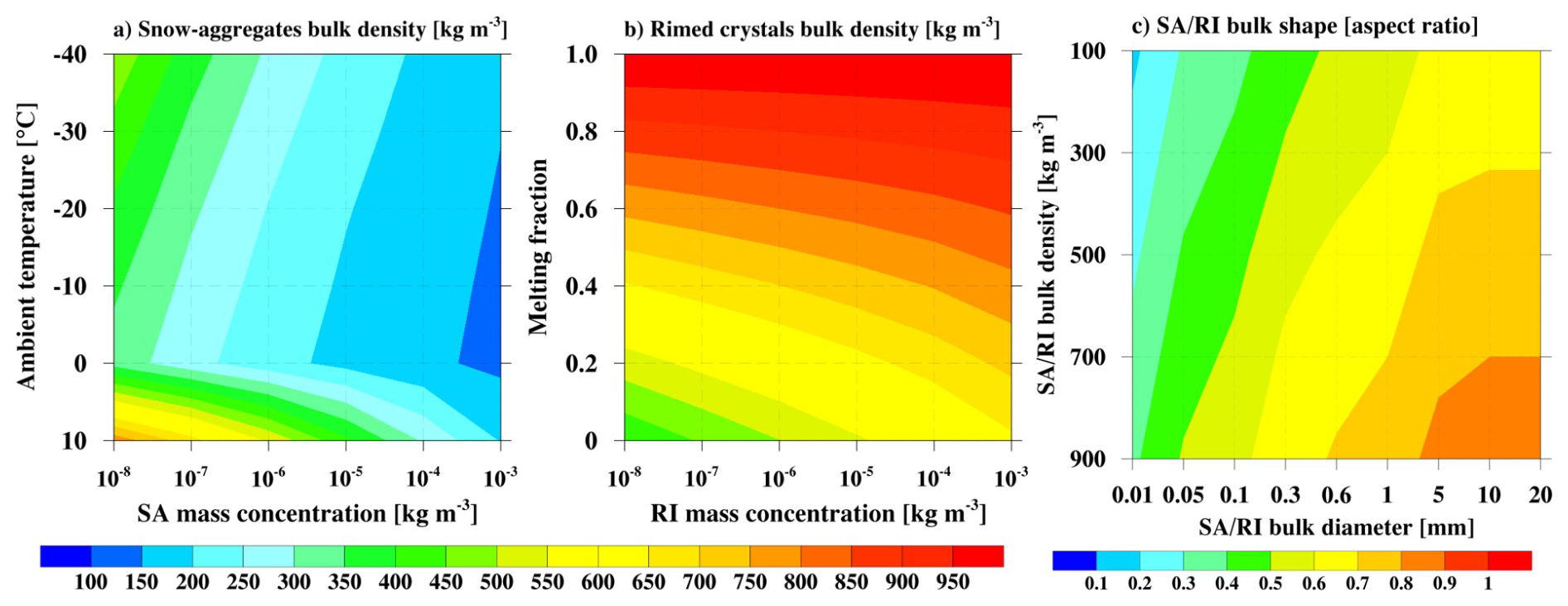
Figure 2 Hydrometeor bulk density (kg m⁻³) as a function of mass concentration (kg m⁻³) for (a) snow aggregates against ambient temperature (°C), and (b) rimed ice against melting fraction. Bulk hydrometeor shape expressed as aspect ratio for snow aggregates and rimed ice, shown as a function of bulk density (kg m⁻³) and bulk diameter (mm) in panel (c).

Finally, TC20 simulations indicate that large SA aspect ratios approach approximately 0.65, while predicted graupel shapes are confined below 0.8 for large oblate particles (Jensen and Harrington, 2015). To ensure morphological consistency among size, density, and shape, TCWA2 employs a generalized diagnostic relation for oblate SA and RI:

$$\begin{array}{}\text{(8)}& {\mathit{\varphi }}_x=a+b\ln {\mathit{\rho }}_x+c\ln {\mathit{\rho }}_x^{\mathrm{2}}+d\ln D_x+e\ln D_x^{\mathrm{2}}+f\ln D_x^{\mathrm{3}}\le \mathrm{1},\end{array}$$

where $x\in \left(\mathrm{s},\mathrm{g}\right)$, ρ_x is the bulk density (kg m⁻³), and D_x is the bulk diameter (µm). As shown in Fig. 2c, the aspect ratio approaches 0.65 for low-density SA and increases toward 0.8 for dense RI at millimeter scales. For sub-millimeter particles, bulk aspect ratios range from approximately 0.1 to 0.5, indicating stronger asphericity at lower densities. Below the freezing level, partial melting further shifts both shape and density toward those of liquid water. Although the above parameterizations are approximations of hydrometeor shape and density, they establish a linkage between microphysical processes and the radar forward operator, thereby allowing for a more objective evaluation of BMPs performance.

Finally, the diagnosed PSD parameters and associated hydrometeor properties must be combined with the particle's terminal velocity to accurately model the sedimentation of bulk moments. TCWA2 employs the theoretical bulk fall speed parameterizations developed by Chen et al. (2022), which explicitly incorporate particle morphology within a multi-moment gamma-type PSD framework. Alternative formulations for each category, based on PSD and morphology, are derived by fitting offline integrations of bin-based calculations. Detailed expressions and fitted coefficients are provided in Appendix A. Note that the ice shape effect has been integrated into the parameterizations of deposition and collision retained from TC20. The parameterization of the number sink due to evaporation loss is revised in Appendix B.

2.3 Bulk dual-polarization radar operator

Radar forward operators have been continuously enhanced to connect NWP models and radar observations, often utilizing precomputed electromagnetic scattering lookup tables or parameterizations based on assumed particle shapes and exponential PSDs. While these methods work for traditional BMPs with fixed or slightly varying spectral parameters, they are not compatible with the physical assumptions underlying TCWA2. Specifically, employing existing radar operators would require externally imposed, internally inconsistent assumptions about PSD shape, particle density, and melting effects. To address this limitation, a new bulk dual-polarization radar operator is developed to explicitly link the gamma-type PSD to the diagnosed α, melting fraction of large ice particles, and category-dependent hydrometeor properties in TCWA2.

Under the Rayleigh approximation, the backward scattering amplitudes $f_{a,b}^{\left(\mathit{\pi }\right)}$ and the forward scattering amplitudes $f_{a,b}^{\left(\mathrm{0}\right)}$ are expressed as follows (Van de Hulst, 1981):

$$\begin{array}{}\text{(9)}& f_{a,b}^{\left(\mathit{\pi }\right)}=f_{a,b}^{\left(\mathrm{0}\right)}={\displaystyle \frac{{\mathit{\pi }}^{\mathrm{2}}{D}^{\mathrm{3}}}{\mathrm{6}{\mathit{\lambda }}_a}}{\displaystyle \frac{\mathrm{1}}{L_{a,b}+\frac{\mathrm{1}}{\mathit{\epsilon }-\mathrm{1}}}},\end{array}$$

where λ_a is the radar wavelength, D is the equivolume particle diameter, and ε is the dielectric constant determined by the ice-liquid fraction. The depolarization factors L_a,b correspond to oblate or prolate spheroids and depend on particle aspect ratio (Ryzhkov et al., 2011). Although the Rayleigh approximation is formally valid only for particles small compared to the radar wavelength, Ryzhkov et al. (2011) estimated that the associated errors are typically within ∼ 1 dBZ for reflectivity and 0.1–0.2 dB for Z_DR at S- and C-band frequencies, given cutoff equivolume diameters ranging from 3.6 to 8 mm. These uncertainties are substantially smaller than those arising from PSD variability and microphysical assumptions in BMPs. Moreover, TCWA2 employs flexible gamma-type PSDs with diagnostically varying α, which suppress the large-diameter tail relative to the Marshall–Palmer spectrum (α=0), thereby reducing resonance effects associated with large particles.

In traditional bulk radar operators, particle-level scattering amplitudes f_a,b are often approximated as power-law functions of particle diameter, then integrated over an assumed PSD (e.g., Jung et al., 2008). While this method can achieve reasonable accuracy for radar reflectivity, its effectiveness would decline for polarimetric variables such as Z_DR and K_DP, which are expressed as ratios or differences between two bulk scattering integrals. In such cases, small fitting errors in the particle-level f_a,b may be nonlinearly amplified during subtraction or division, leading to a loss of numerical significance (i.e., large-term cancellation). To avoid this issue, TCWA2 adopts a different strategy. Instead of fitting particle-level f_a,b, bulk dual-polarimetric radar variables are obtained directly from bin-based scattering calculations integrated over the PSD following Ryzhkov et al. (2011, Eq. 29). Specifically, bin calculations are performed over hydrometeor-dependent, model-resolved ranges of PSD parameters (100 combinations of α_x and λ_x), and the resulting bulk radar signatures of D_BZ,x, Z_DR,x, K_DP,x for each category $x\in \left(\mathrm{r},\mathrm{i},\mathrm{s},\mathrm{g}\right)$ are then fitted as functions of the spectral parameters (α_x, λ_x,N_x), hydrometeor properties (φ_x, ρ_x), and radar wavelength (λ_a=0.11 m for S band and 0.053 m for C band). By directly fitting radar signatures constrained to the PSD variability range in TCWA2, the accuracy of the simulated radar outputs mainly relies on the fitted bulk parameterizations, thus avoiding numerical errors from intermediate calculations.

Matsui et al. (2019) demonstrated that simulated dual-polarimetric observables are highly sensitive to assumptions about particle shape, orientation, and tumbling. In TCWA2, hydrometeors are assumed to have a fixed equilibrium orientation, with no explicit canting-angle variability, tumbling, or electric-field-induced alignment. Nonspherical particles fall with their maximum dimensions aligned horizontally, corresponding to an orientation angle of 90° measured from the vertical to the particle's major axis. This broadside-falling assumption is consistent with microphysical calculations of collision cross section and fall speed, but it may enhance the simulated dual-polarimetric response because orientation randomization is not represented. The radar operator also uses a fixed horizontal-viewing geometry at a zero-elevation angle. Therefore, elevation-angle-dependent projection effects are not represented and may introduce uncertainty when comparing with radar observations at nonzero elevation angles. Lastly, the bulk apparent density and aspect ratios of SA and RI are treated as modal-mean properties independent of particle size, while the shapes of RD and PI explicitly vary with particle diameter, allowing the aspect ratio to change across the PSD for a given bulk mean size. This distinction is especially important for polarimetric variables, as spectral variability in particle shape strongly impacts Z_DR and K_DP. Although size–shape dependence has received limited attention in previous bulk radar operators, it is explicitly incorporated in the TCWA2 operator to ensure physically consistent polarimetric signals.

After evaluating the sensitivity to individual variables, the horizontal reflectivity factor Z_H,x for category x is parameterized as

$$\begin{array}{}\text{(10)}& Z_{\mathrm{H},x}\cong N_{x}f\left({\mathit{\rho }}_x\right){\mathrm{10}}^{\mathrm{0.1}{D}_{\mathrm{BZ},x}-\mathrm{18}},\end{array}$$

with a coefficient of determination (R²) reaching 0.9998. The fitted expressions for D_BZ,x with the density correction function f(ρ_x) are provided in Appendix C1. Since the Z_DR is defined as the ratio of horizontal to vertical reflectivity, the vertical reflectivity factor Z_V,x for category x is then derived from

$$\begin{array}{}\text{(11)}& Z_{\mathrm{V},x}={\displaystyle \frac{Z_{\mathrm{H},x}}{{\mathrm{10}}^{\mathrm{0.1}{Z}_{\mathrm{DR},x}}}},\end{array}$$

where Z_DR,x depends on both PSD parameters and hydrometeor properties. The specific differential phase K_DP,x for category x is expressed as a function of number concentration, PSD parameters, hydrometeor properties, and radar wavelength (λ_a, with a reference of 0.11 m):

$$\begin{array}{}\text{(12)}& K_{\mathrm{DP},x}\cong N_{x}f\left({\mathit{\alpha }}_x,{\mathit{\lambda }}_x\right)f\left({\mathit{\rho }}_x\right)f\left({\mathit{\varphi }}_x\right){\displaystyle \frac{\mathrm{0.11}}{{\mathit{\lambda }}_a}},\end{array}$$

with the fitted formulations of Z_DR,x and K_DP,x for each category, as given in Appendices C2 and C3 (R² > 0.9919). For wet SA and RI, direct fitting to mixed-phase PSDs is difficult because particles in both groups contain both ice and liquid components. TCWA2, therefore, adopts a mean-size approximation in which particle shape and density are linearly weighted by the melting mass fraction f_mw. The dielectric constant of wet ice particles, ε_wx, is computed using a two-step Maxwell–Garnett mixing formulation (Maxwell Garnett, 1904) and fitted as a function of bulk density and volume water fraction, f_vw.

$$\begin{array}{}\text{(13)}& {\mathit{\epsilon }}_{\mathrm{w}x}=a+b{f}_{\mathrm{vw}}^{-\mathrm{1}}+c{\mathit{\rho }}_x+d{f}_{\mathrm{vw}}^{-\mathrm{2}}+e{\mathit{\rho }}_x^{\mathrm{2}}+f{\mathit{\rho }}_x{f}_{\mathrm{vw}}^{-\mathrm{1}},\end{array}$$

where $x\in \left(\mathrm{s},\mathrm{g}\right)$, and the coefficients are listed in Table 1. The volume water fraction f_vw follows Ryzhkov et al. (2011, Eq. 10), incorporating ice density effects and modified with a water-skin exponent from Jung et al. (2008, Eq. 2):

$$\begin{array}{}\text{(14)}& f_{\mathrm{vw}}={\left({\displaystyle \frac{{\mathit{\rho }}_x{f}_{\mathrm{mw}}}{{\mathit{\rho }}_{\mathrm{w}}-{\mathit{\rho }}_{\mathrm{w}}{f}_{\mathrm{mw}}+{\mathit{\rho }}_x{f}_{\mathrm{mw}}}}\right)}^{\mathrm{0.3}},\end{array}$$

with D_BZ,x, Z_DR,x, and K_DP,x computed for each hydrometeor category, the total bulk radar variables are obtained by summation:

$$\begin{array}{}\text{(15)}& {\displaystyle }{D}_{\mathrm{BZ}}=\mathrm{10}\log \mathrm{10}\left[{\mathrm{10}}^{\mathrm{18}}\left(Z_{\mathrm{H},\mathrm{r}}+Z_{\mathrm{H},\mathrm{i}}+Z_{\mathrm{H},\mathrm{s}}+Z_{\mathrm{H},\mathrm{g}}\right)\right]\text{(16)}& {\displaystyle }{Z}_{\mathrm{DR}}=\mathrm{10}\log \mathrm{10}\left({\displaystyle \frac{Z_{\mathrm{H},\mathrm{r}}+Z_{\mathrm{H},\mathrm{i}}+Z_{\mathrm{H},\mathrm{s}}+Z_{\mathrm{H},\mathrm{g}}}{Z_{\mathrm{V},\mathrm{r}}+Z_{\mathrm{V},\mathrm{i}}+Z_{\mathrm{V},\mathrm{s}}+Z_{\mathrm{V},\mathrm{g}}}}\right)\text{(17)}& {\displaystyle }{K}_{\mathrm{DP}}=K_{\mathrm{DP},\mathrm{r}}+K_{\mathrm{DP},\mathrm{i}}+K_{\mathrm{DP},\mathrm{s}}+K_{\mathrm{DP},\mathrm{g}}\end{array}$$

Although TCWA2 is a double-moment scheme with several diagnostic parameterizations, it provides an internally consistent representation of PSD variability, particle morphology, and sedimentation within an integrated framework. Additionally, the dedicated bulk dual-polarization radar operator is derived from bin-based scattering integrations and fitted over the model-resolved PSD space, offering numerical robustness, consistency with the microphysical assumptions, and computational efficiency suitable for online NWP applications.

Table 1 The coefficients for Eqs. (3), (6), (7), (8), and (13).

3 WRF idealized simulations

To examine the physical behavior of the TCWA2 microphysics parameterization, a two-dimensional idealized squall-line simulation is performed using the WRF model. The model setup follows TC20 with 601 horizontal grid points at 1 km spacing and 80 vertical levels. The simulation is initialized with the Weisman and Klemp (1982, 1984) sounding and integrated for 6 h using a 4 s time step, and the model outputs are generated every 10 min. All physical schemes except microphysics are disabled to isolate the effects of the microphysics parameterization. Section 3.1 presents the spatial distributions of diagnosed microphysical variables for each precipitating hydrometeor, followed by an analysis of the corresponding dual-polarimetric radar products in Sect. 3.2.

3.1 Diagnostic variables

The diagnostic variables parameterized in TCWA2 include the spectral shape and aspect ratio, both of which depend on the bulk size and hydrometeor number concentration. Figure 3 shows the instant spatial distributions of number concentration for all categories during the mature stage of the simulated squall-line system. For CD, the number concentration N_c is primarily distributed around the melting layer (below the 0 °C isotherm) and within the convective region (Fig. 3a), with magnitudes on the order of 10⁸ kg⁻¹. The RD number concentration N_r reaches about 10³ kg⁻¹ within the convective core and decreases to 10² kg⁻¹ over the stratiform region (Fig. 3b), displaying a spatial pattern similar to that of CD but extending to lower altitudes. For PI, the number concentration N_i is highest in the upper cloud region around 10⁴ kg⁻¹ and gradually decreases to 10² kg⁻¹ toward the mixed-phase region (Fig. 3c). A local enhancement of N_i appears near the mixed-phase zone, due to secondary ice production. The number concentrations of SA and RI exhibit spatial distributions similar to that of PI but with higher magnitudes, reaching approximately 10⁵ kg⁻¹ for N_s (Fig. 3d) and 10⁴ kg⁻¹ for N_g (Fig. 3e).

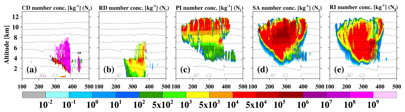
Figure 3 Spatial distributions of the number concentration (kg⁻¹) for (a) cloud droplets, (b) raindrops, (c) pristine ice, (d) snow aggregates, and (e) rimed ice (from left to right) at 6 h of simulation time. The horizontal and vertical axes denote horizontal distance and altitude (km), respectively. Black dashed lines indicate air temperature isotherms from 20 to −50 °C at 10 °C intervals.

Figure 4a shows that raindrops are suspended within the convective core up to about 6 km in altitude, with peak diameters of roughly 1 mm located below the melting layer. In contrast, smaller bulk diameters are found over the stratiform region, reflecting weaker collision processes. For PI, the mean diameters near the cloud top are generally smaller than 0.15 mm and increase to around 0.2 mm as particles fall toward the mixed-phase region (Fig. 4b). Overall, the diameter distributions of SA and RI exhibit growing variability from the upper anvil region down to the melting layer (Fig. 4c, d), consistent with gravitational size sorting. Note that the wet SA and RI appear below the melting layer to represent partial melting, and the RI's diameter continuously increases to 1 mm. Larger particle diameters are seen along the cloud edges, likely due to sublimation effects aloft. In addition, active collision processes are present within the convective region above the melting layer, where the SA and PI, which have relatively low fall speeds, are more often collected by the RD.

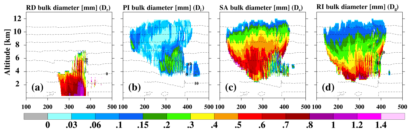
Figure 4 Same as Fig. 3, but showing the bulk diameter (mm) for (a) raindrops, (b) pristine ice, (c) snow aggregates, and (d) rimed ice.

For RD, the α_r in Fig. 5a approaches 1 near the melting layer and within the convective core, indicating relatively broad PSDs in the accretion-dominated region. In the stratiform region without the presence of the CD, the α_r slightly increases to 2 due to evaporation through the switch to diffusion mode. For PI, the α_i remains below 1 within the upper anvil, reflecting small ice particles in the diffusion-dominated region (Fig. 5b). As particles descend into the mixed-phase region, α_i increases beyond 1, indicating depositional growth and reduced N_i. The α_s and α_g show similar vertical patterns. Both are less than 1 near the cloud top, pointing to broad PSDs in the anvil region, and gradually rise to about 1.3 above the melting layer through size sorting (Fig. 5c, d). Higher values of α_s and α_g are also observed at cloud edges, due to sublimation removing smaller particles and narrowing the PSD. Finally, α_s and α_g rise sharply, exceeding 20 just below the melting layer, reflecting melting-induced narrowing of the PSD.

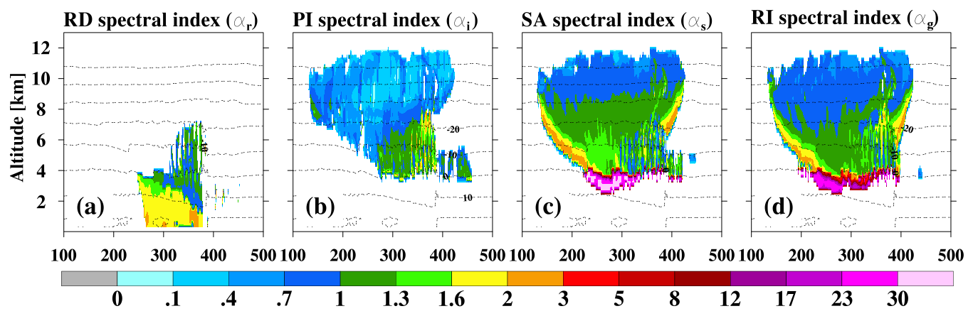
Figure 5 Same as Fig. 3, but showing the spectral shape parameter for (a) raindrops, (b) pristine ice, (c) snow aggregates, and (d) rimed ice.

In Fig. 6a, the bulk ice density ρ_i remains nearly constant at 910 kg m⁻³ as solid ice. For SA, the ρ_s starts around 400 kg m⁻³ near the cloud top and gradually decreases to 100 kg m⁻³ as particle mass increases (Fig. 6b). This feature reflects the formation of low-density, porous particles through aggregation. In contrast, the ρ_g also begins near 400 kg m⁻³ in the upper cloud region and increases to 700 kg m⁻³ with increasing particle mass (Fig. 6c), indicating that enhanced riming produces more compact particle structures. Below the melting layer, both ρ_s and ρ_g exhibit locally elevated values due to partial melting, which increases particle compactness and effective density as liquid water accumulates on ice particles (Fig. 6b, c). The relatively low ρ_g near the convective core can be partly attributed to the diagnostic treatment of RI density in TCWA2. The SLL parameterization provides a practical approach, but it may require further refinement as more observational constraints become available. Overall, the bulk density distributions in TCWA2 illustrate distinct growth pathways of deposition, aggregation, and riming for three groups of ice particles, respectively.

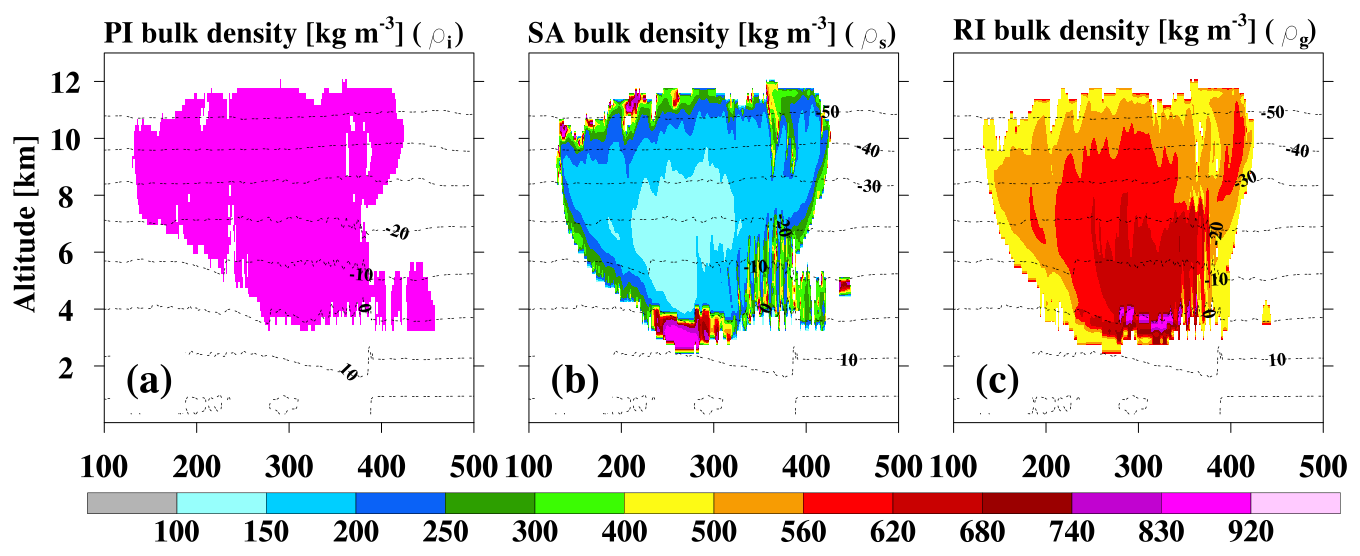
Figure 6 Same as Fig. 3, but showing the bulk apparent density (kg m⁻³) for (a) pristine ice, (b) snow aggregates, and (c) rimed ice.

Figure 7a presents that the RD aspect ratio φ_r is about 0.9 within the convective core and increases toward unity in the stratiform region. For PI, the aspect ratio φ_i is parameterized using the temperature-dependent habit function Γ(T), leading to distinct shape transitions with height. Columnar ice crystals dominate at temperatures colder than −20 °C, while plate-like habits are prevalent between −10 and −20 °C. Above −10 °C, the ice habit shifts back toward columnar types (Fig. 7b). Consequently, the φ_i varies widely from 7 to 0.1. For oblate SA, the aspect ratio φ_s indicates highly aspherical particles (∼ 0.4) in the upper cloud region, and gradually increases to 0.6 near the melting layer through ice aggregation (Fig. 7c). The RI φ_g shows systematically larger aspect ratios, increasing to about 0.8 below the melting layer due to liquid water partitioning during melting (Fig. 7d).

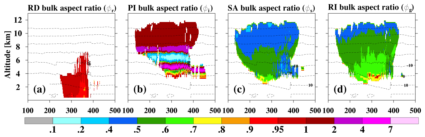
Figure 7 Same as Fig. 3, but showing the bulk aspect ratio (shape) for (a) raindrops, (b) pristine ice, (c) snow aggregates, and (d) rimed ice.

To demonstrate the relationship between hydrometeor properties and bulk fall speed, Fig. 8 displays the mass-weighted fall speed as a function of bulk diameter for four precipitation categories. The RD bulk fall speed rises quickly for diameters smaller than 2 mm and gradually levels off at about 8 m s⁻¹. This damping behavior results from increased drag caused by large drop deformation when φ_r falls below 0.8. For PI, the bulk fall speed varies significantly, mainly influenced by crystal shape. Particles with more aspherical habits (i.e., larger deviations of φ_i from one) fall more slowly, as shown by the orange and purple points, while more spherical crystals (φ_i close to one), represented by the blue points, attain higher fall speeds. This emphasizes the high sensitivity of PI sedimentation to habit-dependent effects. The bulk fall speed of SA shows a consistent dependence on particle density, increasing steadily from low- to medium-density aggregates. Additionally, RI displays a similar density-dependent relationship but with extra scatter influenced by particle shape. Overall, RD has the highest average bulk fall speed (3.71 m s⁻¹), followed by RI (0.85 m s⁻¹), SA (0.46 m s⁻¹), and PI (0.16 m s⁻¹), which aligns more closely with the traditional method using fixed parameters prescribed for specific hydrometeors (i.e., Locatelli and Hobbs, 1974).

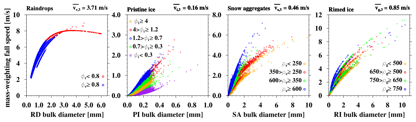
Figure 8 Scatter plots of bulk mass-weighted fall speed (m s⁻¹) by bulk diameter (mm) for raindrops, pristine ice, snow aggregates, and rimed ice (from left to right). Points are color-coded by bulk aspect ratio and bulk density. Data are sampled over the simulation period from 1 to 6 h. Mean values are indicated in the upper-right corner of each panel.

Although TCWA2 captures the main features of variable PSDs, regime-dependent microphysical variables, and property-dependent fall speeds, the diagnostic approach used here is inevitably less complex than the NTU scheme, which explicitly tracks particle growth memory through prognostic moments.

3.2 Dual-polarimetric radar products

The dual-polarimetric radar variables of D_BZ, Z_DR, and K_DP are parameterized in TCWA2 as functions of the PSD, hydrometeor properties, and number concentration. This subsection investigates the spatial distribution of these radar products in the simulated convective system and explains how individual hydrometeors contribute to polarimetric signatures.

Figure 9 presents the spatial distributions of simulated horizontal radar reflectivity (D_BZ) along with its breakdown into contributions from RD, PI, SA, and RI. The total radar reflectivity (Fig. 9a) depicts a deep convective structure marked by strong echoes exceeding 40 dBZ that extend from near the surface up to about 7 km altitude, followed by a downstream shift to a stratiform region around 260 km in horizontal distance. Below the melting layer, RD dominates the reflectivity signal, highlighting the role of melting ice particles in generating large liquid drops associated with the radar bright band (Fig. 9b). Above the freezing level, SA mainly contributes to the outflow cloud deck reflectivity (0–25 dBZ), reflecting efficient aggregation within the main ice cloud region (Fig. 9d). In contrast, RI accounts for the enhanced reflectivity (> 20 dBZ) in the mixed-phase region, indicative of active riming (Fig. 9e). The PI contribution is relatively weak (< 0 dBZ) and mostly confined to upper levels, due to its small particle size (Fig. 9c). This hydrometeor-based breakdown reveals a clear vertical partitioning of reflectivity linked to deposition, aggregation, riming, and melting processes in TCWA2.

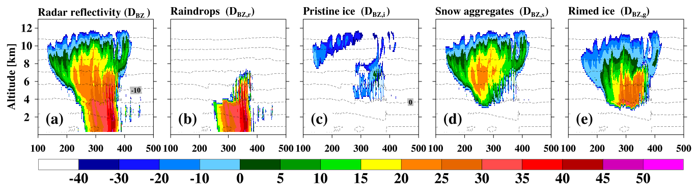
Figure 9 Spatial distributions of horizontal radar reflectivity (dBZ) at 6 h of simulation time. Panels from left to right indicates the (a) total signal and contributions from (b) raindrops, (c) pristine ice, (d) snow aggregates, and (e) rimed ice. The horizontal and vertical axes denote horizontal distance and altitude (km), respectively. Black dashed lines indicate air temperature isotherms from 20 to −50 °C at 10 °C intervals.

Figure 10 illustrates the spatial distribution of simulated differential reflectivity (Z_DR) and highlights three common polarimetric features seen in convective systems. First, a prominent Z_DR column (Illingworth et al., 1987; Loney et al., 2002) appears just below and above the freezing level, mainly caused by RD (Fig. 10b). This feature results from large, oblate liquid drops lifted by strong updrafts and from reduced particle terminal velocity. It is well represented by the diameter-dependent RD shape, the fall speed formulation, and the flexible PSD modeling in TCWA2. Second, a midlevel Z_DR band (Kumjian and Ryzhkov, 2008) about 1 dB appears in the melting layer, caused by partially melted SA and RI with increased bulk density during melting (Fig. 10d, e). Third, a clear cloud-top Z_DR enhancement (> 1 dB) is simulated at higher levels, mainly due to PI (Fig. 10c). Elevated Z_DR in this zone indicates the presence of columnar solid ice crystals with relatively low fall speeds. Throughout the broader cloud deck, Z_DR remains relatively low (0.1–0.4 dB), mostly due to SA, given the dominant reflectivity partition. Although PI shows high Z_DR values locally within the mixed-phase region, its contribution to the total Z_DR is much less than that of RI.

Figure 10 Same as Fig. 9, but showing the differential reflectivity (dB).

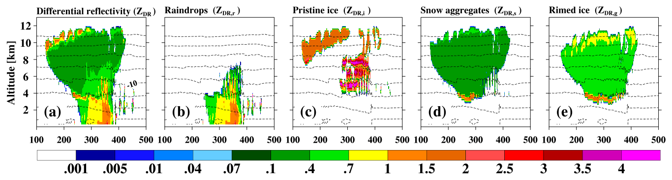
Figure 11 presents vertical cross sections of simulated specific differential phase (K_DP) and reveals a distinct KDP column (Hubbert et al., 1998; Loney et al., 2002) stretching from near the surface through the mixed-phase region into upper levels at 7 km, collocated with the strongest updrafts. This feature is mainly caused by RI within the mixed-phase region and by RD below the freezing level (Fig. 11b, e). The continuous enhancement of K_DP along the vertical indicates the presence of many aspherical, dense hydrometeors lifted by strong upward motion. In addition, these particles contribute to localized K_DP (> 0.4 ° km⁻¹) near the melting layer. Above the freezing layer, K_DP remains relatively weak across various cloud decks and is mostly associated with dry SA (Fig. 11d). Contribution from PI at temperatures warmer than −40 °C is generally minor due to its low number concentration (Fig. 11c).

Figure 11 Same as Fig. 9, but showing the specific differential phase at C band (° km⁻¹).

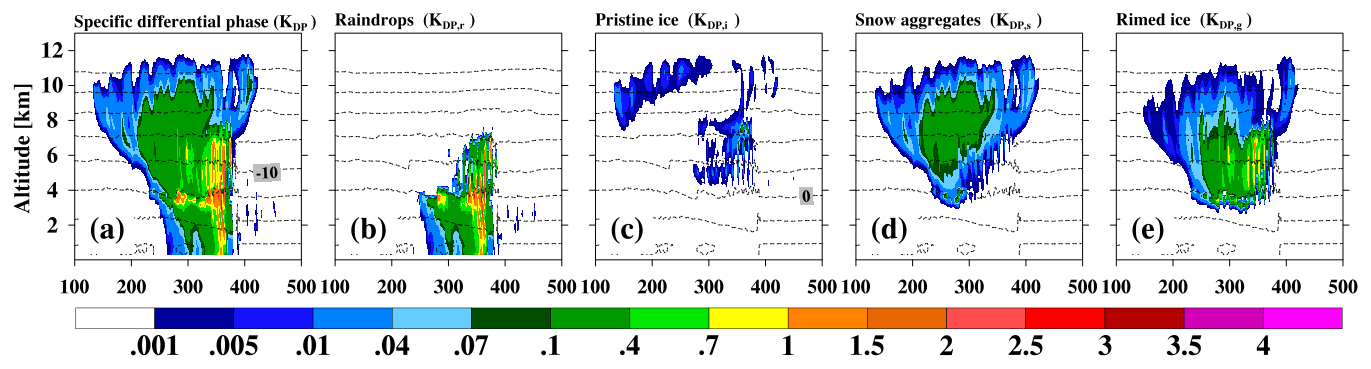
Figure 12 further demonstrates how Z_DR depends on spectral shape, aspect ratio, and apparent density for each type of hydrometeor. For RD, Z_DR steadily rises with bulk diameter and reaches higher (lower) values for smaller (larger) α_r at the same diameter, indicating more (less) deformation in broader (narrower) PSDs. For PI, Z_DR varies greatly at small diameters, mainly influenced by particle shape, with highly aspherical crystals producing higher Z_DR despite weaker reflectivity. Dry SA typically results in small Z_DR values that decrease as diameter increases, while wet SA shows moderate Z_DR that quickly declines as particles become denser and more spherical during melting. Similarly, dry RI particles have low Z_DR, and wet RI falls within the intermediate Z_DR range.

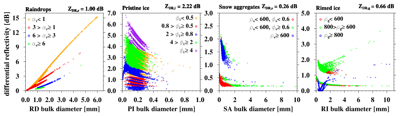
Figure 12 Same as Fig. 8, but showing the differential reflectivity (dB). Points are color-coded by the spectral shape, bulk aspect ratio, and bulk density, respectively.

In summary, these results show that TCWA2 consistently performs across PSD variability, microphysical diagnostics, sedimentation behavior, and polarimetric radar products, and provides a physical foundation for applying TCWA2 to proof-of-concept real-case simulations and radar-based model assessments discussed in later sections.

4 Proof-of-concept real-case demonstration using MPAS

The purpose of this section is not to provide a comprehensive operational validation or scheme intercomparison, but rather to demonstrate that the TCWA2 framework can be stably integrated into a three-dimensional model and produce physically interpretable polarimetric signatures. The MPAS model is adopted for real-case simulations because its unstructured-mesh framework enables seamless multiscale representation of convective systems within a single, globally consistent domain, while avoiding the lateral boundary issues that are inherent in limited-area models such as WRF. Additionally, the limited availability of only two microphysics schemes (WSM6 and Thompson) in MPAS is another strong reason to implement TCWA2 within the MPAS framework to facilitate broader application and evaluation.

4.1 Model setup and cases

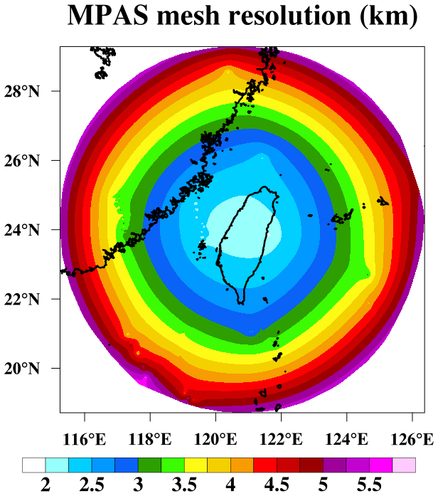
The MPAS model is configured with a variable-resolution mesh comprising 97 031 horizontal cells, with the model top at 30 km. The mesh includes a circular refinement zone centered at (24.0° N, 121.0° E) with a radius of 850 km. Inside this area, a high horizontal resolution of 2 km is maintained within about a 150 km radius, gradually expanding to 6 km toward the outer edges. This setup covers roughly 18.7–29.2° N in latitude and 115.3–126.8° E in longitude (Fig. 13), covering the operational radar network over Taiwan. The 2 km grid spacing is coarser than the 1 km idealized WRF simulation and may underresolve convective-core updrafts and hydrometeor lofting. Thus, this real-case convection-permitting simulation is suitable for evaluating overall precipitation organization and qualitative polarimetric structures, but it should not be interpreted as a complete assessment of TCWA2 behavior within fully resolved convective cores. For time integration, the model uses a 36 s time step with 4 acoustic sub-steps (the default is 2) to ensure numerical stability and high-resolution efficiency. For physical parameterizations, the scale-aware New Tiedtke cumulus scheme (Wang, 2022) is used to ensure consistent performance across different mesh resolutions. Boundary layer and surface processes are represented by the Yonsei University PBL scheme (Hong et al., 2006) and Monin–Obukhov similarity theory (Monin and Obukhov, 1954), respectively. Land-surface interactions and radiative transfer are handled through the Noah Land Surface Model (Chen and Dudhia, 2001) and the RRTMG scheme (Iacono et al., 2008). To provide reference context rather than a definitive scheme intercomparison, additional simulations are performed using the single-moment WSM6 (Hong and Lim, 2006) and semi-double-moment Thompson (Thompson et al., 2008) schemes, alongside the TCWA2 simulation.

Figure 13 MPAS model domain and horizontal mesh resolution (km).

For the case study, an afternoon thunderstorm observed during the TAHOPE field campaign on 24 June 2022, was selected for evaluation. This event involved a typical convective system that caused precipitation over western central Taiwan, with a maximum of over 190 mm accumulated within 12 h. The heavy rainfall and well-developed leading convective structure make this case ideal for assessing microphysical performance using ground-based radar data. Each experiment started at 00:00 UTC on 24 June 2022, and lasted for 12 h, with initial and boundary conditions provided by the National Centers for Environmental Prediction (NCEP) Global Forecast System (GFS). Model outputs are compared with two observational datasets. First, precipitation forecasts are verified against ground-based observations from the CWA's Quantitative Precipitation Estimation and Segregation Using Multiple Sensors (QPESUMS) system (Chang et al., 2021). Second, simulated polarimetric radar variables are contrasted with Plan Position Indicator (PPI) observations from four operational CWA radar sites: RCWF (25.07° N, 121.77° E; S band), RCLY (22.53° N, 120.38° E; C band), RCNT (24.14° N, 120.58° E; C band), and RCSL (25.0° N, 121.4° E; C band). These radar stations collectively cover the leading convective areas of the event. During this thunderstorm, a leading squall line formed around 06:00 UTC on 24 June and dissipated by approximately 11:00 UTC. Accordingly, six-hourly radar data were sampled to match the model output frequency. The results are analyzed with particular focus on the characteristics of dual-polarimetric radar variables.

4.2 Simulation evaluations

The simulation results are assessed using a hierarchy of precipitation, reflectivity, and dual-polarimetric diagnostics. Figure 14 displays three simulations that generally replicate the elongated north–south precipitation band over western and central Taiwan, with spatial pattern correlations between 0.53 and 0.55. The mean of the highest 10 precipitation values is 198 mm for WSM6, 188 mm for Thompson, and 173 mm for TCWA2, compared with 181 mm for QPESUMS. The WSM6 run produces a larger area of intense rainfall exceeding 90 mm over central Taiwan, indicating it overestimates the most intense precipitation amounts. Thompson and TCWA2 generate a narrower distribution of heavy rainfall, closer to the observed value, for this metric.

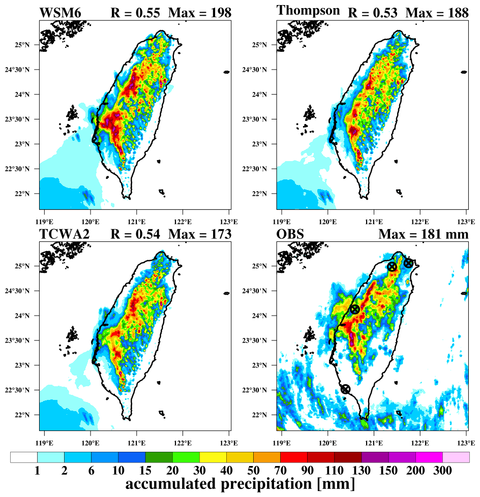
Figure 14 Spatial distributions of 12 h accumulated precipitation (mm) simulated using the WSM6, Thompson, and TCWA2 microphysics schemes, compared with QPESUMS observations. The pattern correlation for each run is indicated at the top of each panel, along with the average precipitation of the highest 10 points. The locations of the RCWF (25.07° N, 121.77° E), RCLY (22.53° N, 120.38° E), RCNT (24.14° N, 120.58° E), and RCSL (25.0° N, 121.4° E) radar sites are marked by black circles in the rightmost panel.

As the location of the leading convective system is identified, a comprehensive evaluation is performed using grid-to-grid comparison against hourly radar observations from 06:00 to 11:00 UTC at four radar stations. Figure 15 shows joint height–D_BZ probability density distributions comparing simulated and observed D_BZ. The observed joint distribution displays a frequent occurrence of reflectivity values between 2–10 km altitude, with reflectivity values mainly ranging from 10 to 30 dBZ. Above the melting layer near 5 km altitude, reflectivity steadily decreases with height, indicating ice growth through riming and aggregation. Enhanced reflectivity exceeding 30 dBZ around 5 km corresponds to the radar bright band caused by the melting of large ice particles. The WSM6 simulation captures the overall vertical structure but has a broader distribution of high reflectivity, suggesting an overproduction of large hydrometeors. The Thompson scheme shows better vertical coherence compared to WSM6 but still has an overly extended high reflectivity region below 5 km, especially near the bright band peak. The pronounced bright band signatures may partly result from the combined effects of the fixed ice-particle density assumptions in the microphysics schemes and the simplified treatment of dielectric properties during melting in the radar operator. In contrast, the TCWA2 run shows the closest agreement with the observations, achieving a pattern correlation of 0.99. The vertical placement and intensity of the reflectivity core depict a realistic transition from moderate reflectivity at lower levels, to peak echoes within the melting layer, and to weaker values aloft. Notably, the reflectivity value around 25 dBZ and the enhanced bright band signals at 4–5 km altitude are captured in both narrow and broad PSD representations. The lower occurrence of moderate reflectivity at upper levels may be related to the current RI initiation treatment or the lack of accumulated riming-history memory, and warrants further examination in future work. Nevertheless, this improved depiction suggests that TCWA2 more effectively constrains the hydrometeor PSD through microphysical growth and sedimentation processes, offering a robust baseline for subsequent assessment of dual-polarimetric radar variables.

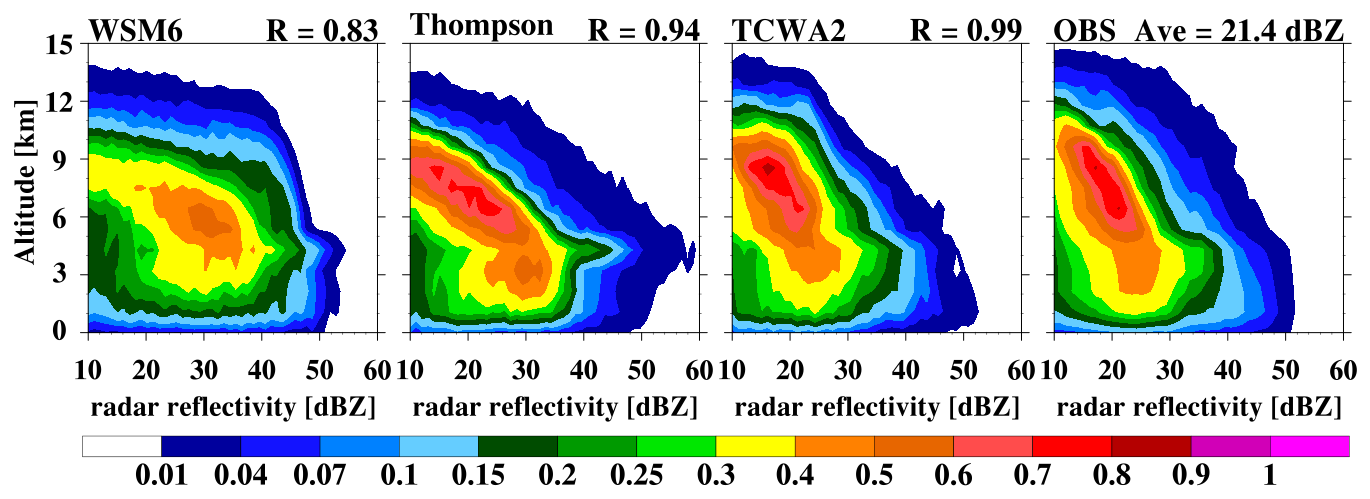
Figure 15 Joint probability density distribution of height (km) and horizontal radar reflectivity (dBZ) for simulations using the WSM6, Thompson, and TCWA2 microphysics schemes, compared with observations. The pattern correlation between simulated and observed joint distribution is indicated at the top of each panel, along with the observed mean reflectivity magnitude from the CWA measurements.

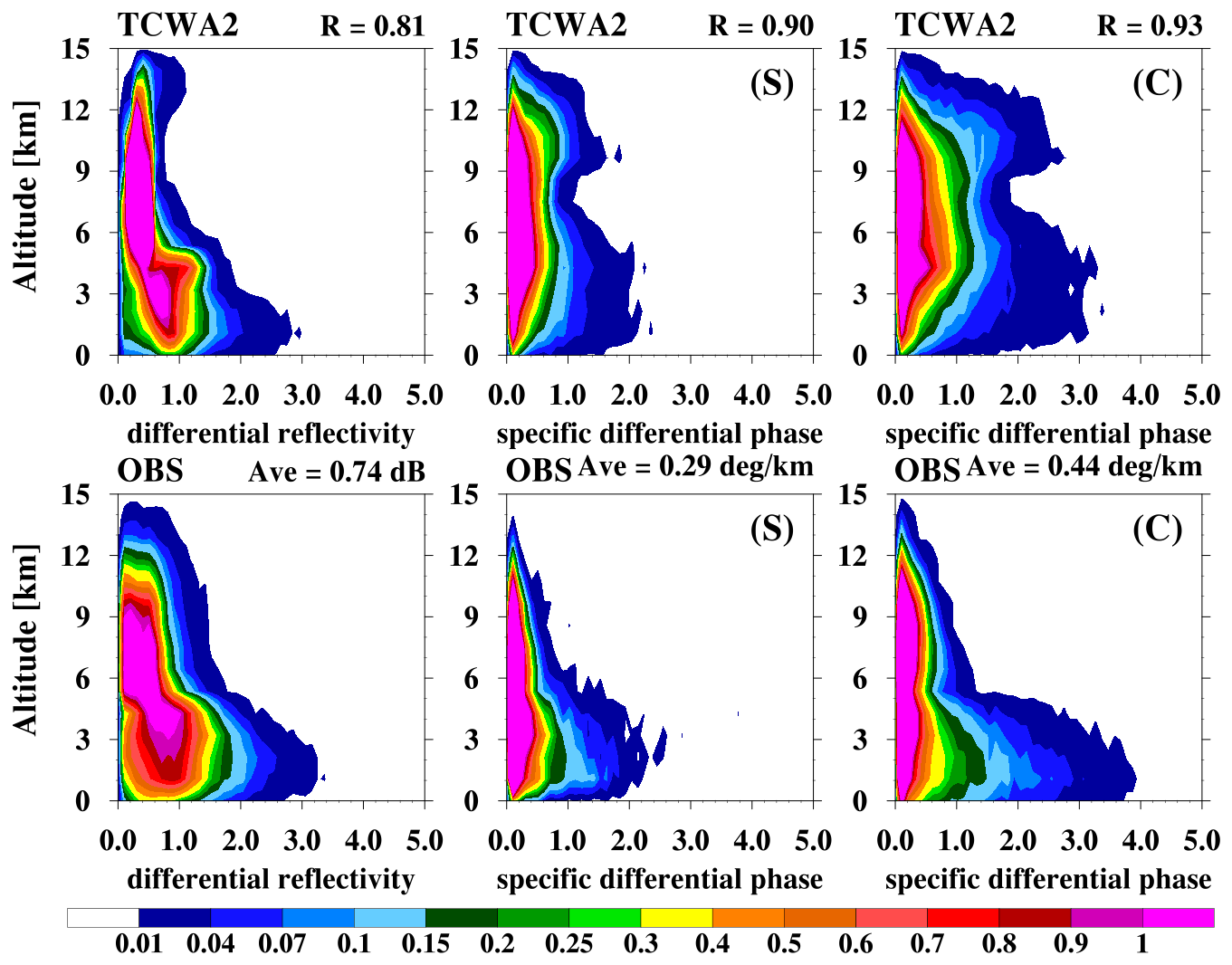
Figure 16 Joint probability density distribution from the TCWA2 simulation (top row) and the corresponding observations (bottom row). The radar variables shown from left to right are differential reflectivity (dB), specific differential phase at S band (° km⁻¹), and specific differential phase at C band (° km⁻¹). The pattern correlation between simulated and observed distribution is indicated at the top of each panel, along with the observed mean values from the CWA measurements.

To further compare the dual-polarimetric radar products simulated by TCWA2, Fig. 16 shows joint distribution comparisons of Z_DR and K_DP between the TCWA2 simulation and observations. The observed joint height–Z_DR features a concentrated core between 0.1 and 1.5 dB below 4 km altitude, with a near-surface tail extending toward 3 dB, indicating the presence of oblate RD in a broad spectrum, along with size-sorting processes. Above the melting layer, the Z_DR core diminishes below 1 dB and gradually weakens with height up to about 15 km. A slightly enhanced Z_DR signal appears above 12 km in the TCWA2 simulation from the aspherical PI on the cloud top. Overall, the TCWA2 simulation generally reproduces both the vertical confinement and magnitude of the Z_DR core, with a pattern correlation of 0.81. Since the K_DP value depends on the radar wavelength, comparisons are performed separately for S and C band observations, corresponding to different sampling points. Both joint height–K_DP comparisons show similar levels of agreement. Observations reveal enhanced K_DP below 5 km, with maxima extending toward the surface, reflecting high liquid water content and active collisional breakup processes. TCWA2 captures this vertical distribution with pattern correlations of 0.90 and 0.93 for the two K_DP configurations, respectively. However, TCWA2 occasionally overestimates K_DP near 10 km altitude, which may partly reflect limitations in the microphysical parameterizations of RI, the fixed horizontal-viewing geometry, and the broadside-falling assumption for particle orientation without explicit tumbling or electric-field-induced alignment. These uncertainties indicate the need for further refinement.

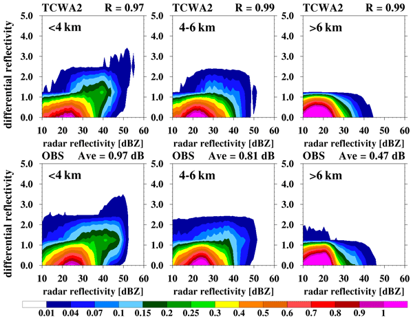
To account for distinct microphysical regimes and isolate the influence of melting-layer processes, the simulated and observed radar signatures are analyzed by stratifying the results to assess whether the simulated raindrop and ice-particle characteristics align with observations at various heights. Figure 17 illustrates the joint distribution of Z_DR and D_BZ by dividing them into three altitude ranges. In the low-level region below 4 km, observations show multiple Z_DR modes associated with liquid-phase hydrometeors. A primary Z_DR core is centered around 0.2 dB within 20–30 dBZ, along with a broader distribution below 1 dB across 10–35 dBZ. A secondary mode with higher Z_DR values, reaching about 2 dB, appears between 30 and 45 dBZ, likely related to increases in RD accretion and self-collection. Occasional instances exceeding 2.5 dB above 40 dBZ are also observed, with this significant deformation mainly caused by melting of large oblate ice particles in a broad PSD. The TCWA2 simulation closely reproduces both the magnitude and variability of the observed Z_DR–D_BZ relationship dominated by RD. Within the mixed-phase layer between 4 and 6 km, the observed Z_DR cores for strong reflectivity (> 40 dBZ) are substantially reduced, while sporadic Z_DR enhancements (around 0.1–0.15) are contributed by partial melting into liquid drops. TCWA2 effectively simulates this transition from rain-dominated conditions to mixed-phase wet SA and RI across the melting layer. Above 6 km, both observations and simulations exhibit low Z_DR and D_BZ values, generally below 1 dB and 30 dBZ, consistent with near-spherical ice particles. TCWA2 captures key aspects of this pattern, achieving a pattern correlation of 0.99. The relative magnitude of Z_DR against D_BZ is broadly consistent with the expected influence of ice-phase hydrometeor properties. However, this interpretation remains sensitive to radar-operator assumptions such as particle orientation and viewing geometry. Overall, the agreement between simulated and observed Z_DR–D_BZ distributions across all altitude ranges provides encouraging evidence that TCWA2 can represent key aspects of the vertical evolution of hydrometeor size and shape in this convective system.

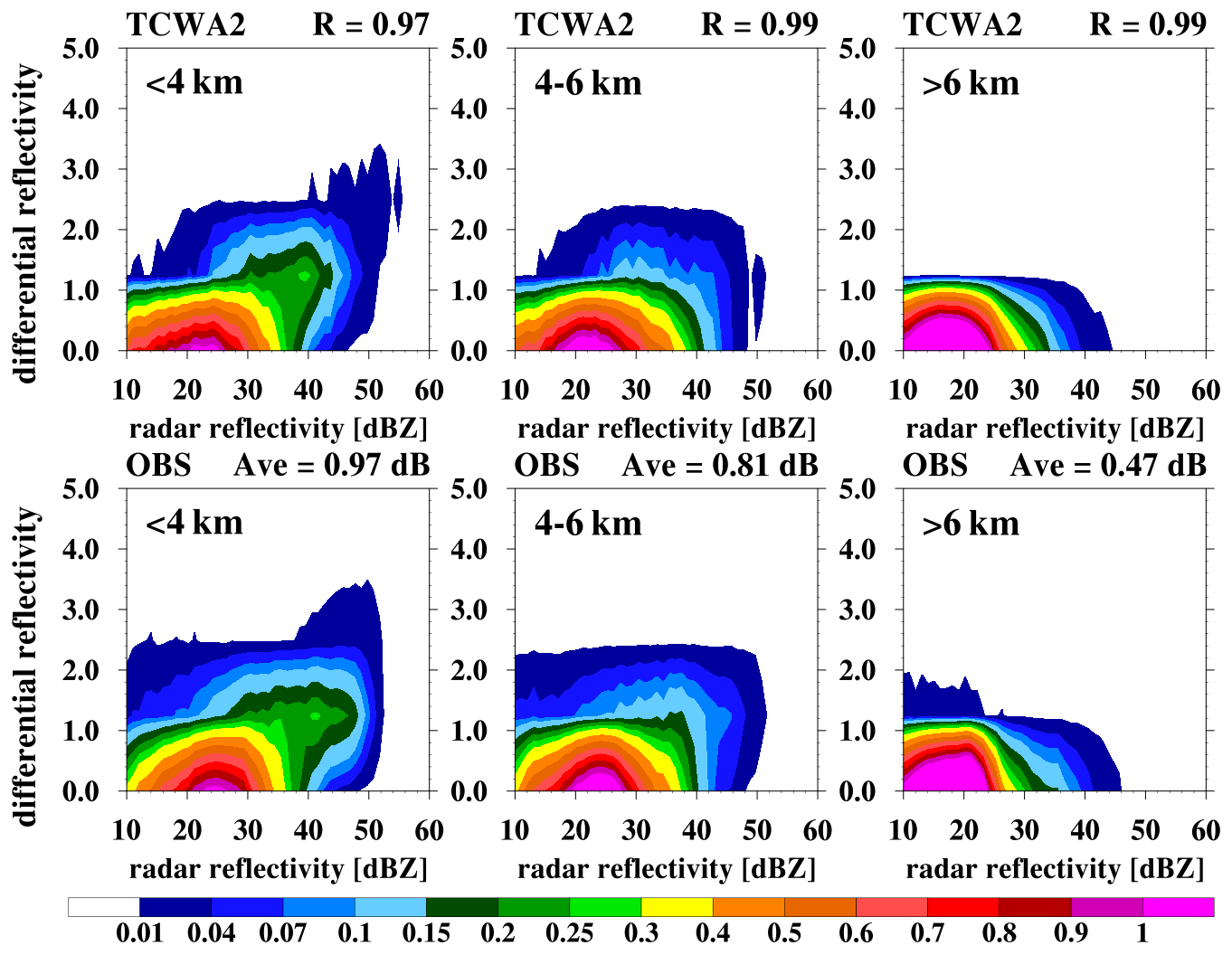
Figure 17 Height-stratified joint probability density distribution of differential reflectivity (dB) as a function of radar reflectivity (dBZ) from the TCWA2 simulation (top row) and the corresponding observations (bottom row). Panels are grouped by altitude ranges: low (< 4 km), middle (4–6 km), and upper (> 6 km). Pattern correlations are indicated at the top of each TCWA2 panel, along with the observed mean Z_DR values.

Figure 18 further depicts the joint distributions of K_DP at S band against D_BZ by dividing the results into three altitude zones. Since K_DP is directly proportional to the number concentration of nonspherical particles, this analysis offers a strict constraint on how the number density related to asphericity is represented. In the low-altitude region below 4 km, observations exhibit a main distribution centered near 30 dBZ and ranging roughly from 10 to 50 dBZ, with most K_DP values staying below 1° km⁻¹. A secondary population with higher K_DP reaching up to 2.5° km⁻¹ appears at strong reflectivity over 45 dBZ, mainly from large melting oblate ice particles. The TCWA2 simulation produces a narrower core between 30 and 40 dBZ and occasionally overestimates K_DP at reflectivities above 40 dBZ. However, it still captures the observed relationship between K_DP and D_BZ. In the mixed-phase layer between 4 and 6 km, the observed K_DP distribution has a similar shape, but with lower peak values and less frequent occurrences, reflecting a smaller amount of liquid water confined to partial melting. TCWA2 replicates this weaker K_DP signal during phase changes. Above 6 km, both observations and simulations show low K_DP and D_BZ values, generally under 1° km⁻¹ and 45 dBZ, aligned with ice-dominated hydrometeors and minimal liquid water occurrence. Although TCWA2 matches the overall pattern of the observed distribution, the simulated core shifts slightly from the observed 10–25 dBZ range to 15–30 dBZ. This bias is probably caused by uncertainties in observational sampling with S-band radar at a relatively long distance from the convective system.

Figure 18 Same as Fig. 17, but showing the specific differential phase at S band (° km⁻¹).

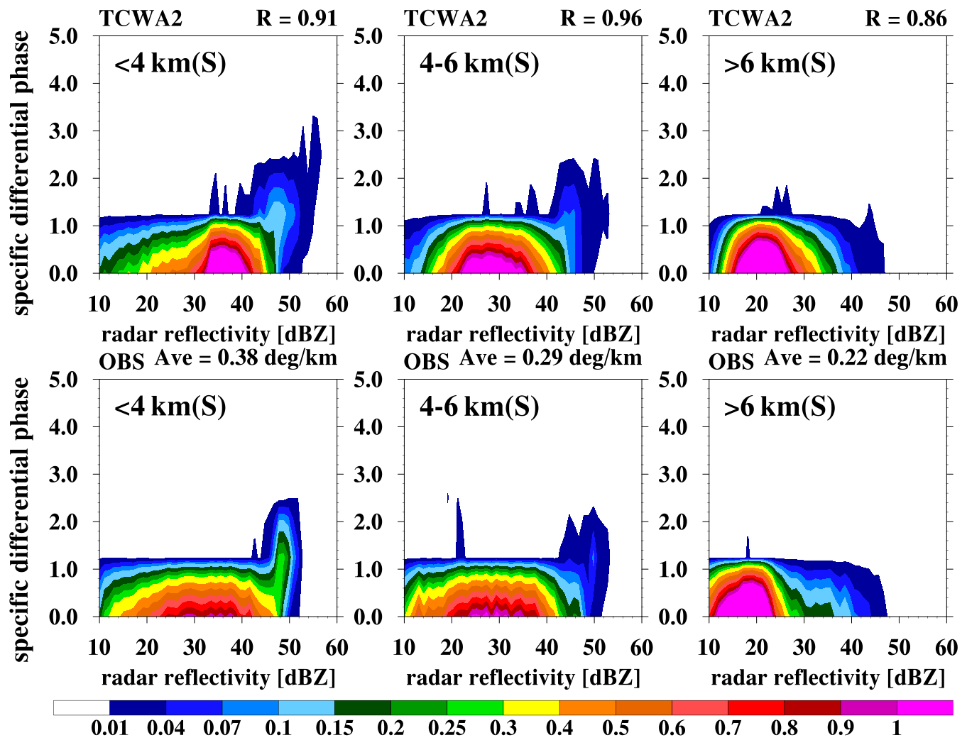
Figure 19 shows the joint distributions of K_DP and D_BZ at C band, divided by altitude, offering an independent assesment of the simulated hydrometeor signatures with a shorter radar wavelength. Compared to S-band data, C-band K_DP is more sensitive to raindrop size and number concentration. In the low-level layer below 4 km, observations reveal a dominant K_DP core within 30–40 dBZ, mostly below 1° km⁻¹, with noticeable K_DP increases when reflectivity exceeds 30 dBZ. Peak K_DP values reach about 5° km⁻¹ and occur more often at high reflectivity than in S-band data, reflecting the stronger wavelength dependence of K_DP at C band. The TCWA2 simulation closely reproduces both the magnitude and reflectivity dependence of the observed distribution. In the layer between 4 and 6 km, where mixed-phase hydrometeors are present, observed K_DP values decline and become more tightly clustered, reflecting diminishing liquid water content and phase changes. TCWA2 captures this vertical shift of melting and liquid water depletion across the melting layer with a pattern correlation of 0.97. Above 6 km, both observations and simulations show weak K_DP values, generally below 1° km⁻¹, consistent with ice-dominated hydrometeors and limited supercooled liquid water. Although there are occasional discrepancies with K_DP over 1° km⁻¹, possibly associated with RI signatures and radar-operator assumptions. Nevertheless, TCWA2 captures the overall distribution, with a high pattern correlation of 0.98.

Figure 19 Same as Fig. 17, but showing the specific differential phase at C band (° km⁻¹).

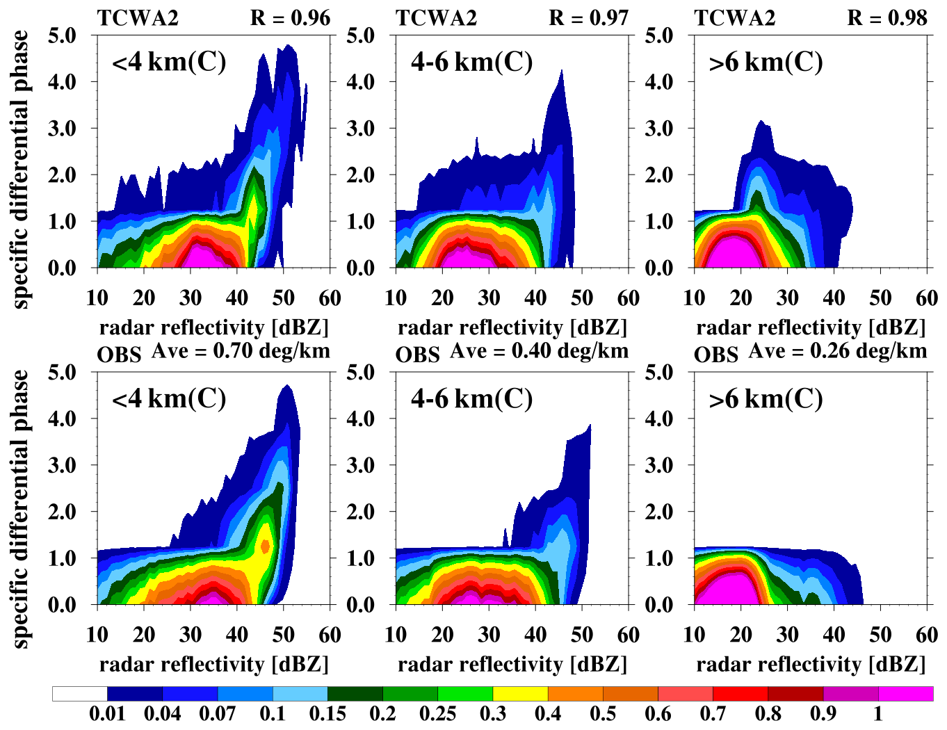
The MPAS real-case analysis is intended as a proof-of-concept demonstration, not as a comprehensive operational validation or definitive scheme intercomparison. The simulations show that TCWA2 captures key aspects of the observed vertical reflectivity patterns and height-dependent dual-polarization signatures, with encouraging pattern correlations. However, discrepancies remain at upper levels and may partly reflect observational limitations, ice-phase uncertainties in the RI parameterizations, the fixed horizontal-viewing geometry in the radar operator, the broadside-falling particle-orientation assumption, and the absence of explicit tumbling or canting-angle variability. These issues remain topics for future process-level evaluation.

All simulations were run with MPI parallelization across 32 CPU cores. The total wall-clock times, with microphysics-component times in parentheses, were 402 (22), 511 (34), and 550 (118) s for the WSM6, Thompson, and TCWA2 simulations, respectively. Compared with Thompson, the TCWA2 microphysics component required about 3.5 times as much computational time, primarily due to revised parameterizations and additional calculations of dual-polarization radar variables. However, the total wall-clock time increased by only 39 s, or about 7.6 %, in this model configuration. Thus, TCWA2 remains computationally practical because it retains a double-moment prognostic framework while diagnosing additional microphysical and radar-related properties.

5 Summary

This study introduces TCWA2, a double-moment bulk cloud microphysics scheme designed for operational weather prediction that utilizes dual-polarimetric radar observations at the Taiwan CWA. By emulating the triple-moment NTU scheme, TCWA2 preserves a gamma-type PSD with adjustable spectral shape parameters, diagnoses hydrometeor-related properties, and revises the number sinks during diffusional loss. Additionally, TCWA2 incorporates theoretically based fall-speed formulations that account for particle density and aspect ratio, allowing the assessment of how PSD variation and particle morphology affect sedimentation processes. To connect the gaps between BMPs and radar diagnostics, this study further develops a customized bulk dual-polarization radar operator based on offline bin-based scattering calculations integrated over the model PSD range using the Rayleigh approximation.

The idealized WRF squall-line simulation illustrates the spatial distribution of microphysical diagnostics, the physical behavior of parameterized variables, and the leading factors on bulk fall speeds for each hydrometeor. The simulated polarimetric variables show interpretable spatial features, and the contributions of individual precipitating categories to the dual-polarimetric radar products are quantified through decomposition analysis. Key radar signatures, including the melting layer bright band, K_DP column, and Z_DR column, are well reproduced. Additionally, the role of size-shape dependence in determining raindrop Z_DR in terms of different spectral shape parameters is specifically highlighted.

For the proof-of-concept MPAS real-case simulation of an afternoon thunderstorm event on 24 June 2022 during the TAHOPE field campaign, comparisons with observed precipitation and radar reflectivity indicate that the TCWA2 scheme captures the convective system's geographic distribution and vertical structure. The joint probability density distribution analysis of Z_DR and K_DP shows generally consistent behavior, despite some overestimation in the upper levels. In particular, the joint distributions of radar reflectivity and polarimetric variables show encouraging agreement with observations, with pattern correlations exceeding 0.9 across three altitude layers. These results suggest that TCWA2 and its embedded bulk radar operator can capture key radar-signature characteristics associated with liquid-, mixed-, and solid-phase hydrometeors. However, remaining discrepancies may partly reflect uncertainties associated with ice-phase parameterizations, simplified broadside-falling particle-orientation assumptions, and the fixed radar-viewing geometry. These issues indicate the need for further evaluation and future refinement.

In summary, the TCWA2 scheme provides a foundation for data assimilation, as radar-relevant hydrometeor properties are accessible from the microphysics parameterization and are formulated consistently with the radar operator. The bulk particle terminal velocities diagnosed by TCWA2 allow for process-level validation against observed radial velocities. Additionally, the distinct microphysical properties among different categories and their corresponding polarimetric radar signatures provide interpretable guidance for radar-based hydrometeor classification algorithms. This physically consistent formulation of the radar forward operator can help reduce representativeness errors and enhance convective-scale short-term forecasts when assimilating dual-polarimetric radar observations. Consequently, the bulk dual-polarization radar operator has been integrated into the MPAS-JEDI (Joint Effort for Data assimilation Integration) system for future radar data assimilation tasks.

Appendix A: Parameterizations of bulk fall speed and parameters

A1 Bulk moment-weighting fall speed

The generalized expression for the bulk fall speed associated with the kth moment is parameterized as

$$\begin{array}{}\text{(A1)}& \begin{array}{rl}& v_{x,k}=R_x\exp \\ & \left(\begin{array}{l}{a}_x+b_x{y}_{x,k}+c_x{z}_x+d_x{y}_{x,k}^{\mathrm{2}}+e_x{z}_x^{\mathrm{2}}+f_x{y}_{x,k}{z}_x\\ +g_x{y}_{x,k}^{\mathrm{3}}+h_x{z}_x^{\mathrm{3}}+i_x{y}_{x,k}{z}_x^{\mathrm{2}}+j_x{y}_{x,k}^{\mathrm{2}}{z}_x\end{array}\right)\\ & f\left({\mathit{\rho }}_x\right)f\left({\mathit{\varphi }}_x\right)f\left({\mathit{\rho }}_{\mathrm{a}}\right)\end{array}\end{array}$$

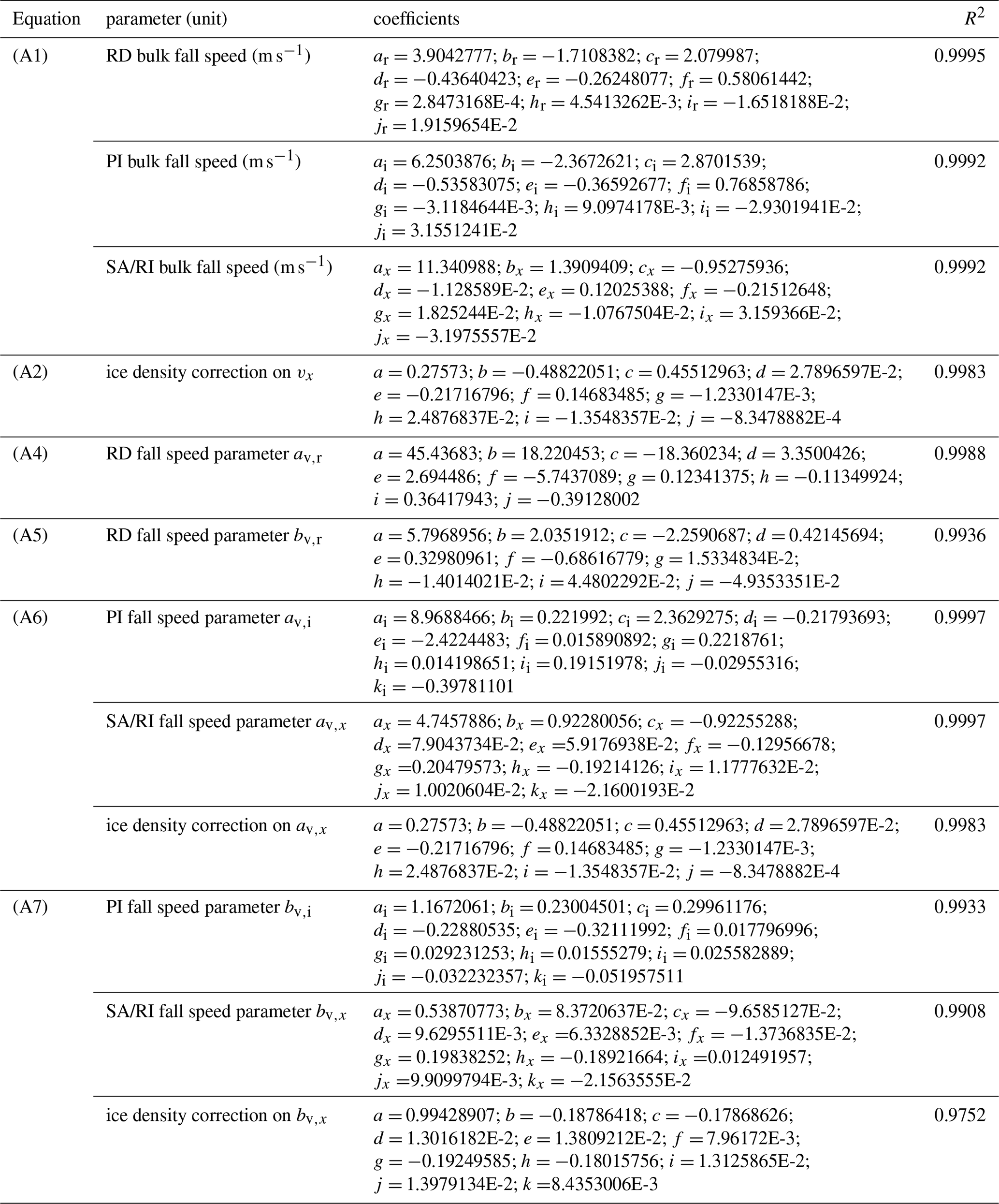
where $x\in \left(\mathrm{r},\mathrm{i},\mathrm{s},\mathrm{g}\right)$, $k\in \left(\mathrm{0},\mathrm{3}\right)$ represents the moment order, $y_{x,k}=\ln \left({\mathit{\alpha }}_x+\mathrm{2}+k\right)$, and z_x=ln λ_x. The air density correction f(ρ_a) follows Heymsfield et al. (2007). The scaling factor R_x is set to 10⁻⁵ for PI and 10⁻³ for the remaining categories. The density correction is unity for RD. For ice particles, it is parameterized as

$$\begin{array}{}\text{(A2)}& f\left({\mathit{\rho }}_x\right)=\left(\begin{array}{l}a+b{y}_x+c{z}_x+d{y}_x^{\mathrm{2}}+e{z}_x^{\mathrm{2}}+f{y}_x{z}_x\\ +g{y}_x^{\mathrm{3}}+h{z}_x^{\mathrm{3}}+i{y}_x{z}_x^{\mathrm{2}}+j{y}_x^{\mathrm{2}}{z}_x\end{array}\right)\le \mathrm{1},\end{array}$$

where $x\in \left(\mathrm{i},\mathrm{s},\mathrm{g}\right)$, y_x=ln D_x, and z_x=ln ρ_x.

The shape correction f(ϕ_x) is unity for RD, and ${\mathit{\varphi }}_x^{\mathrm{1}/\mathrm{3}}$ for SA and RI. For PI, the correction depends on crystal habit $f\left({\mathit{\varphi }}_{\mathrm{i}}\right)=D_{\mathrm{i}\mathrm{0}}^{\mathit{\zeta }/\mathrm{2}}$ and $y_{x,i}=\ln \left({\mathit{\alpha }}_{\mathrm{i}}+\mathit{\zeta }+\mathrm{2}+k\right)$ for prolate crystals, whereas $f\left({\mathit{\varphi }}_{\mathrm{i}}\right)=D_{\mathrm{i}\mathrm{0}}^{-\mathit{\zeta }}$ and $y_{x,i}=\ln \left({\mathit{\alpha }}_{\mathrm{i}}-\mathit{\zeta }/\mathrm{2}+\mathrm{2}+k\right)$ for oblate crystals. $\mathit{\zeta }=\left(\mathit{\beta }-\mathrm{1}\right)/\left(\mathit{\beta }+\mathrm{2}\right)$ the ice growth ratio (see CT16; TC20).

A2 Bulk fall speed parameters for ventilation effects

In addition to the moment-weighted fall speed described in Appendix A1, fall-speed parameters are necessary to determine the ventilation factor (e.g., vapor diffusional and melting processes). The bulk terminal velocity for hydrometeor category x is represented by a power-law form.

$$\begin{array}{}\text{(A3)}& v_x=a_{\mathrm{v},x}{D}_x^{b_{\mathrm{v},x}},\end{array}$$

where a_v,x and b_v,x are the prefactor and exponent parameters, respectively, derived according to the parameterization of Khvorostyanov and Curry (2002).

A2.1 Raindrops

For RD, the parameters of a_v,r and b_v,r are separately expressed as

$$\begin{array}{}\text{(A4)}& {\displaystyle }{a}_{\mathrm{v},\mathrm{r}}=\exp \left(\begin{array}{l}a+b{y}_{\mathrm{r}}+c{z}_{\mathrm{r}}+d{y}_{\mathrm{r}}^{\mathrm{2}}+e{z}_{\mathrm{r}}^{\mathrm{2}}+\\ f{y}_{\mathrm{r}}{z}_{\mathrm{r}}+g{y}_{\mathrm{r}}^{\mathrm{3}}+h{z}_{\mathrm{r}}^{\mathrm{3}}+i{y}_{\mathrm{r}}{z}_{\mathrm{r}}^{\mathrm{2}}+j{y}_{\mathrm{r}}^{\mathrm{2}}{z}_{\mathrm{r}}\end{array}\right),\text{(A5)}& {\displaystyle }\begin{array}{rl}{b}_{\mathrm{v},\mathrm{r}}& =a+b{y}_{\mathrm{r}}+c{z}_{\mathrm{r}}+d{y}_{\mathrm{r}}^{\mathrm{2}}+e{z}_{\mathrm{r}}^{\mathrm{2}}+f{y}_{\mathrm{r}}{z}_{\mathrm{r}}+g{y}_{\mathrm{r}}^{\mathrm{3}}\\ & +h{z}_{\mathrm{r}}^{\mathrm{3}}+i{y}_{\mathrm{r}}{z}_{\mathrm{r}}^{\mathrm{2}}+j{y}_{\mathrm{r}}^{\mathrm{2}}{z}_{\mathrm{r}},\end{array}\end{array}$$

where $y_{\mathrm{r}}=\ln \left({\mathit{\alpha }}_{\mathrm{r}}+\mathrm{2}\right)$, and z_r=ln λ_r.

A2.2 Ice particles

For ice-phase species $x\in \left(\mathrm{i},\mathrm{s},\mathrm{g}\right)$, the prefactor a_v,x is parameterized as

$$\begin{array}{}\text{(A6)}& \begin{array}{rl}{a}_{\mathrm{v},x}& =\exp \left(\begin{array}{l}a+b{y}_x+c{z}_x+d{y}_x^{\mathrm{2}}+e{z}_x^{\mathrm{2}}+f{y}_x{z}_x\\ +g{y}_x^{\mathrm{3}}+h{z}_x^{\mathrm{3}}+i{y}_x{z}_x^{\mathrm{2}}+j{y}_x^{\mathrm{2}}{z}_x\end{array}\right)\\ & f\left({\mathit{\rho }}_{xa}\right)f\left({\mathit{\varphi }}_x\right),\end{array}\end{array}$$

where, $y_x=\ln \left({\mathit{\alpha }}_x+\mathrm{2}\right)$, and z_x=ln λ_x. The ice density correction f(ρ_xa) applied to a_v,x is

$$\begin{array}{}\text{(A6a)}& \begin{array}{rl}f\left({\mathit{\rho }}_{xa}\right)& =\left(\begin{array}{l}a+b{y}_x+c{z}_x+d{y}_x^{\mathrm{2}}+e{z}_x^{\mathrm{2}}+f{y}_x{z}_x\\ +g{y}_x^{\mathrm{3}}+h{z}_x^{\mathrm{3}}+i{y}_x{z}_x^{\mathrm{2}}+j{y}_x^{\mathrm{2}}{z}_x\end{array}\right)\\ & D_x^{b_{\mathrm{v},x}\left[\mathrm{1}-f\left({\mathit{\rho }}_{xb}\right)\right]},\end{array}\end{array}$$

where y_x=ln D_x, z_x=ln ρ_x. The shape correction f(φ_x) is defined as ${\mathit{\varphi }}_x^{\mathrm{1}/\mathrm{3}}$ for SA and RI, whereas it is $D_{\mathrm{i}\mathrm{0}}^{\mathit{\zeta }/\mathrm{2}}$ for prolate PI and $D_{\mathrm{i}\mathrm{0}}^{\mathit{\zeta }/\mathrm{2}}$ for oblate PI crystals. The exponent b_v,x is given by:

$$\begin{array}{}\text{(A7)}& \begin{array}{rl}& b_{\mathrm{v},x}=\\ & \left({\displaystyle \frac{a+c\ln y_x+e\ln z_x+g\ln y_x^{\mathrm{2}}+i\ln z_x^{\mathrm{2}}+k\ln y_x\ln z_x}{\mathrm{1}+b\ln y_x+d\ln z_x+f\ln y_x^{\mathrm{2}}+h\ln z_x^{\mathrm{2}}+j\ln y_x\ln z_x}}\right)\\ & f\left({\mathit{\rho }}_{xb}\right)\end{array}\end{array}$$

where $x\in \left(\mathrm{i},\mathrm{s},\mathrm{g}\right)$, $y_x=ln\left({\mathit{\alpha }}_x+\mathrm{2}\right)$, and z_x=ln λ_x. The ice density correction f(ρ_xb) applied to b_v,x is

$$\begin{array}{}\text{(A7a)}& \begin{array}{rl}& f\left({\mathit{\rho }}_{xb}\right)=\\ & {\displaystyle \frac{a+c\ln D_x+e\ln {\mathit{\rho }}_x+g\ln D_x^{\mathrm{2}}+i\ln {\mathit{\rho }}_x^{\mathrm{2}}+k\ln D_x\ln {\mathit{\rho }}_x}{\mathrm{1}+b\ln D_x+d\ln {\mathit{\rho }}_x+f\ln D_x^{\mathrm{2}}+h\ln {\mathit{\rho }}_x^{\mathrm{2}}+j\ln D_x\ln {\mathit{\rho }}_x}}\\ & \ge \mathrm{1}\end{array}\end{array}$$

where y_x=ln D_x, z_x=ln ρ_x.

All coefficients appearing in Eqs. (A1)–(A7) are listed in Table A1.

Table A1 The coefficients and determination (R²) for the equations in Appendix A.

Appendix B: Number sink due to vapor diffusional processes

In NWP, phase-change processes such as evaporation and sublimation are vital for regulating cold pool formation and the structure of precipitating systems. However, deriving realistic sink rates for hydrometeor number concentration in BMPs remains challenging, because number sink is less directly proportional to mass lost rate and highly dependent on both environmental conditions and the evolving PSD (Seifert, 2008). Therefore, many current BMPs adopt pragmatic closures that relate the number sink to mass loss by assuming a fixed mean volume size (e.g., Khairoutdinov and Kogan, 2000; Milbrandt and Yau, 2005b; Morrison and Grabowski, 2007). While such assumptions may be adequate for broad PSDs (i.e., small or zero α) associated with drizzle in stratocumulus clouds (Khairoutdinov and Kogan, 2000), they may be inappropriate for heavy convective rain (Seifert, 2008), where PSD shapes vary substantially across different microphysical regimes. Since the α in TCWA2 is adjusted according to the growth regime, a revised treatment of number loss during evaporation and sublimation is necessary to ensure realistic PSD evolution.

The mass change rate of an individual particle due to evaporation or sublimation follows vapor diffusional growth theory (Pruppacher and Klett, 1997):

$$\begin{array}{}\text{(B1)}& {\displaystyle \frac{\mathrm{d}m}{\mathrm{d}t}}=\mathrm{2}\mathit{\pi }A{f}_{\mathrm{v}}\left(D\right)\mathrm{\Delta }S,\end{array}$$

Where D is the diameter, A is a thermodynamic correction factor depending on air temperature and pressure, f_v is the ventilation factor, and ΔS is the supersaturation ratio with respect to water or ice. The particle mass can be expressed as $m=\left(\mathit{\pi }/\mathrm{6}\right){\mathit{\rho }}_x{D}^{\mathrm{3}}$, so the differentiation of Eq. (B1) yields:

$$\begin{array}{}\text{(B2)}& {\displaystyle \frac{\mathrm{d}{D}^{\mathrm{2}}}{\mathrm{d}t}}={\displaystyle \frac{\mathrm{8}}{{\mathit{\rho }}_x}}A\stackrel{\mathrm{‾}}{f_{\mathrm{v}}}\mathrm{\Delta }S,\end{array}$$

where $\stackrel{\mathrm{‾}}{f_{\mathrm{v}}}$ denotes the ventilation coefficient obtained from the modal mean diameter for simplicity. The solution of Eq. (B2) for D= 0 over a model time step Δt represents the threshold diameter for total evaporation or sublimation, which can be solved as follows:

$$\begin{array}{}\text{(B3)}& D_{\ast }=\sqrt{-{\displaystyle \frac{\mathrm{8}}{{\mathit{\rho }}_x}}A\stackrel{\mathrm{‾}}{f_{\mathrm{v}}}\mathrm{\Delta }S\mathrm{\Delta }t}.\end{array}$$

Here, ΔS is negative under subsaturated conditions. Once the threshold diameter is determined, the fraction of particles evaporated or sublimated within the time step can be derived from the incomplete gamma function Γ(α+1, D_∗λ) based on the gamma-type PSD. To ensure numerical consistency between mass and number tendencies, both an upper limit of 0.9 and a variable constraint $\frac{\mathrm{6}\mathrm{d}Q/\mathrm{d}t}{\mathit{\pi }{\mathit{\rho }}_x{D}_{\ast }^{\mathrm{3}}}$ are applied to the number loss fraction, where d$Q/$dt is the evaporation or sublimation mass loss rate. This formulation explicitly accounts for PSD variability across different thermodynamic environments, enabling the calculation of the number sink suitable for BMPs in flexible gamma-type PSDs. However, the above approach cannot be easily extended to melting-induced number loss because the presence of an additional riming kernel prevents deriving an analytical solution for the threshold diameter.

Appendix C: Parameterizations of bulk dual-polarization radar variables

C1 Horizontal radar reflectivity

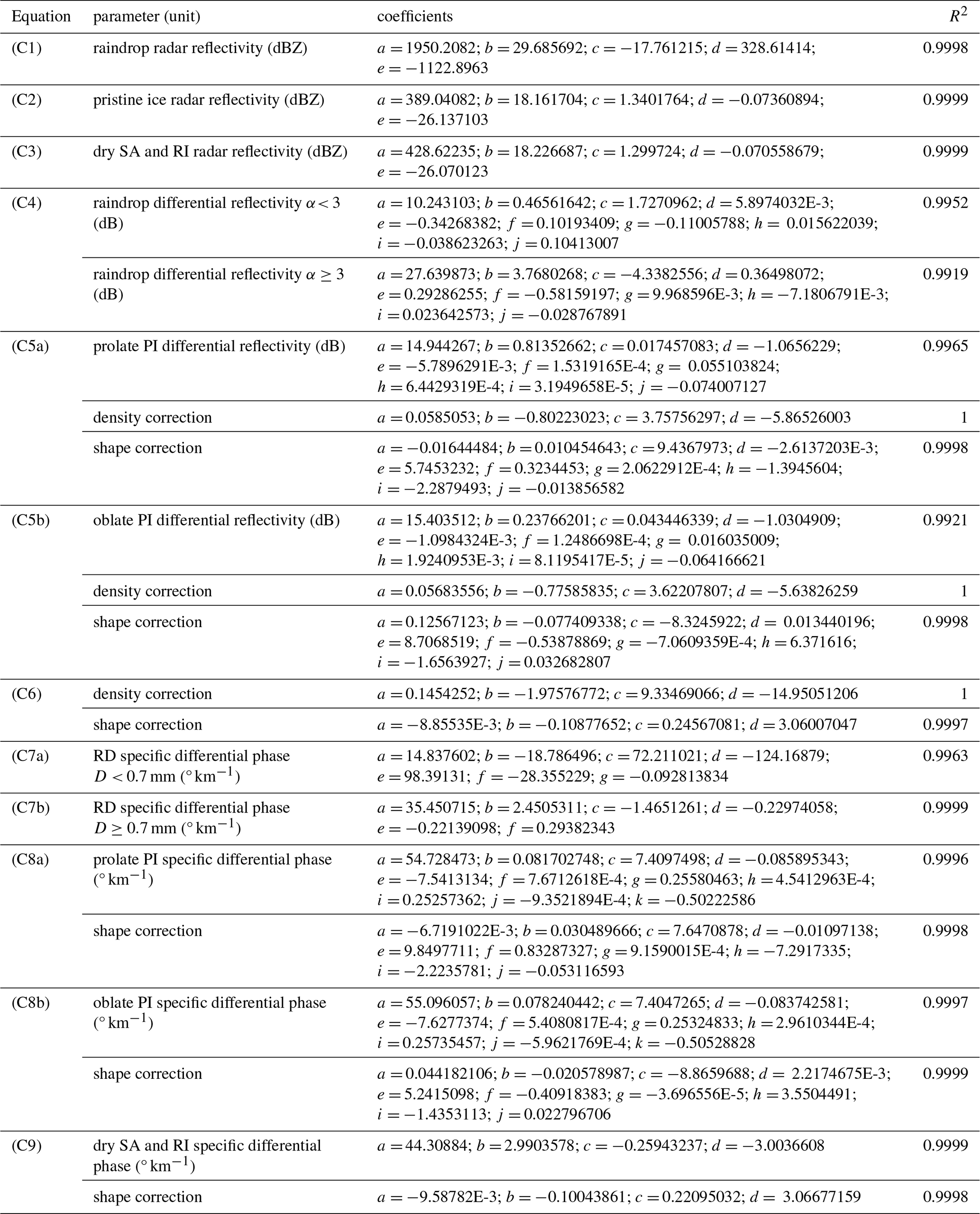
For raindrops (RD), the radar reflectivity is parameterized as

$$\begin{array}{}\text{(C1)}& D_{\mathrm{BZ},\mathrm{r}}=\left(a+b{y}_{\mathrm{r}}+c{y}_{\mathrm{r}}^{\mathrm{0.5}}+d{z}_{\mathrm{r}}^{\mathrm{2}}+e{z}_{\mathrm{r}}^{\mathrm{0.5}}\right)-\mathrm{200},\end{array}$$

where $y_{\mathrm{r}}=\ln \left({\mathit{\alpha }}_{\mathrm{r}}+\mathrm{2}\right)$ and z_r=ln λ_r.

For pristine ice (PI), the density correction is $f\left({\mathit{\rho }}_{\mathrm{i}}\right)=\mathrm{1.9382}\times {\mathrm{10}}^{-\mathrm{6}}{e}^{\mathrm{1.9261}\ln {\mathit{\rho }}_{\mathrm{i}}}$, and the radar reflectivity is given by

$$\begin{array}{}\text{(C2)}& D_{\mathrm{BZ},\mathrm{i}}=\left(a+b{y}_{\mathrm{i}}+c{y}_{\mathrm{i}}^{\mathrm{2}}+d{y}_{\mathrm{i}}^{\mathrm{3}}+e{z}_{\mathrm{i}}\right)-\mathrm{200}.\end{array}$$

For dry snow aggregates (SA) and rimed ice (RI), the density correction is $f\left({\mathit{\rho }}_x\right)=\mathrm{1.544}\times {\mathrm{10}}^{-\mathrm{5}}{e}^{\mathrm{1.95714566}\ln {\mathit{\rho }}_x}$, and the radar reflectivity is parameterized as

$$\begin{array}{}\text{(C3)}& D_{\mathrm{BZ},x}=\left(a+b{y}_x+c{y}_x^{\mathrm{2}}+d{y}_x^{\mathrm{3}}+e{z}_x\right)-\mathrm{250},\end{array}$$

where $x\in \left(\mathrm{s},\mathrm{g}\right)$, $y_x=\ln \left({\mathit{\alpha }}_x+\mathrm{2}\right)$, and z_x=ln λ_x.

C2 Differential reflectivity

For RD, the differential reflectivity is expressed as a function of the PSD:

$$\begin{array}{}\text{(C4)}& \begin{array}{rl}& Z_{\mathrm{DR},\mathrm{r}}={\mathrm{10}}^{-\mathrm{4}}\\ & \exp \left(\begin{array}{l}a+b{y}_{\mathrm{r}}+c{z}_{\mathrm{r}}+d{y}_{\mathrm{r}}^{\mathrm{2}}+e{z}_{\mathrm{r}}^{\mathrm{2}}+f{y}_{\mathrm{r}}{z}_{\mathrm{r}}\\ +g{y}_{\mathrm{r}}^{\mathrm{3}}+h{z}_{\mathrm{r}}^{\mathrm{3}}+i{y}_{\mathrm{r}}{z}_{\mathrm{r}}^{\mathrm{2}}+j{y}_{\mathrm{r}}^{\mathrm{2}}{z}_{\mathrm{r}}\end{array}\right).\end{array}\end{array}$$

For PI, Z_DR,i depends on the ice growth ratio ζ, bulk density ρ_i, and PSD:

$$\begin{array}{}\text{(C5)}& \begin{array}{rl}& Z_{\mathrm{DR},\mathrm{i}}={\mathrm{10}}^{-\mathrm{6}}\\ & \exp \left({\displaystyle \frac{a+b{y}_{\mathrm{i}}+c{y}_{\mathrm{i}}^{\mathrm{2}}+d{z}_{\mathrm{i}}+e{z}_{\mathrm{i}}^{\mathrm{2}}+f{z}_{\mathrm{i}}^{\mathrm{3}}}{\mathrm{1}+g{y}_{\mathrm{i}}+h{y}_{\mathrm{i}}^{\mathrm{2}}+i{y}_{\mathrm{i}}^{\mathrm{3}}+j{z}_{\mathrm{i}}}}\right)f\left({\mathit{\rho }}_{\mathrm{i}}\right)f\left({\mathit{\varphi }}_{\mathrm{i}}\right).\end{array}\end{array}$$

Here, $y_{\mathrm{i}}=\ln \left({\mathit{\alpha }}_{\mathrm{i}}+\mathrm{2}\right)$, z_i=ln λ_i, and D_i is the bulk volume-weighting diameter (m). The density correction is $f\left({\mathit{\rho }}_{\mathrm{i}}\right)=a\ln {\mathit{\rho }}_{\mathrm{i}}^{\mathrm{3}}+b\ln {\mathit{\rho }}_{\mathrm{i}}^{\mathrm{2}}+c\ln {\mathit{\rho }}_{\mathrm{i}}+d$, and the shape correction is $f\left({\mathit{\varphi }}_{\mathrm{i}}\right)=a+b{D}_{\mathrm{i}}+c{\mathit{\zeta }}_{\mathrm{i}}+d{D}_{\mathrm{i}}^{\mathrm{2}}+e{\mathit{\zeta }}_{\mathrm{i}}^{\mathrm{2}}+f{D}_{\mathrm{i}}{\mathit{\zeta }}_{\mathrm{i}}+g{D}_{\mathrm{i}}^{\mathrm{3}}+h{\mathit{\zeta }}_{\mathrm{i}}^{\mathrm{3}}+i{D}_{\mathrm{i}}{\mathit{\zeta }}_{\mathrm{i}}^{\mathrm{2}}+j{D}_{\mathrm{i}}^{\mathrm{2}}{\mathit{\zeta }}_{\mathrm{i}}$.

For dry SA and RI, Z_DR,x is independent of the PSD and given by

$$\begin{array}{}\text{(C6)}& Z_{\mathrm{DR},x}=\mathrm{0.384}f\left({\mathit{\rho }}_x\right)f\left({\mathit{\varphi }}_x\right),\end{array}$$

where $x\in \left(\mathrm{s},\mathrm{g}\right)$. The density correction is $f\left({\mathit{\rho }}_x\right)=a\ln {\mathit{\rho }}_x^{\mathrm{3}}+b\ln {\mathit{\rho }}_x^{\mathrm{2}}+c\ln {\mathit{\rho }}_x+d$, and shape correction is $f\left({\mathit{\varphi }}_x\right)=a\ln {\mathit{\varphi }}_x^{\mathrm{3}}+b\ln {\mathit{\varphi }}_x^{\mathrm{2}}+c\ln {\mathit{\varphi }}_x+d$.

C3 Specific differential phase

For RD, the parameterization of K_DP,r depends on the PSD:

$$\begin{array}{}\text{(C7a)}& {\displaystyle }\begin{array}{rl}& K_{\mathrm{DP},\mathrm{r}}\left(\stackrel{\mathrm{‾}}{D_{\mathrm{r}}}<\mathrm{7}\times {\mathrm{10}}^{-\mathrm{4}}m\right)={\mathrm{10}}^{-\mathrm{10}}\\ & \exp \left(a+{\displaystyle \frac{b}{y_{\mathrm{r}}}}+{\displaystyle \frac{c}{y_{\mathrm{r}}^{\mathrm{2}}}}+{\displaystyle \frac{d}{y_{\mathrm{r}}^{\mathrm{3}}}}+{\displaystyle \frac{e}{y_{\mathrm{r}}^{\mathrm{4}}}}+{\displaystyle \frac{f}{y_{\mathrm{r}}^{\mathrm{5}}}}+g{z}_{\mathrm{r}}\right)\end{array}\text{(C7b)}& {\displaystyle }\begin{array}{rl}& K_{\mathrm{DP},\mathrm{r}}\left(\stackrel{\mathrm{‾}}{D_{\mathrm{r}}}\ge \mathrm{7}\times {\mathrm{10}}^{-\mathrm{4}}m\right)={\mathrm{10}}^{-\mathrm{10}}\\ & \exp \left(a+b{y}_{\mathrm{r}}+c{z}_{\mathrm{r}}+d{y}_{\mathrm{r}}^{\mathrm{2}}+e{z}_{\mathrm{r}}^{\mathrm{2}}+f{y}_{\mathrm{r}}{z}_{\mathrm{r}}\right)\end{array}\end{array}$$

For PI, K_DP,i is parameterized as

$$\begin{array}{}\text{(C8)}& \begin{array}{rl}& K_{\mathrm{DP},\mathrm{i}}=\mathrm{2}\times {\mathrm{10}}^{-\mathrm{18}}\\ & \exp \left({\displaystyle \frac{a+c{y}_{\mathrm{i}}+e{z}_{\mathrm{i}}+g{y}_{\mathrm{i}}^{\mathrm{2}}+i{z}_{\mathrm{i}}^{\mathrm{2}}+k{y}_{\mathrm{i}}{z}_{\mathrm{i}}}{\mathrm{1}+b{y}_{\mathrm{i}}+d{z}_{\mathrm{i}}+f{y}_{\mathrm{i}}^{\mathrm{2}}+h{z}_{\mathrm{i}}^{\mathrm{2}}+j{y}_{\mathrm{i}}{z}_{\mathrm{i}}}}\right)\\ & f\left({\mathit{\rho }}_{\mathrm{i}}\right)f\left({\mathit{\varphi }}_{\mathrm{i}}\right),\end{array}\end{array}$$

with the shape correction $f\left({\mathit{\varphi }}_{\mathrm{i}}\right)=a+b{D}_{\mathrm{i}}+c{\mathit{\zeta }}_{\mathrm{i}}+d{D}_{\mathrm{i}}^{\mathrm{2}}+e{\mathit{\zeta }}_{\mathrm{i}}^{\mathrm{2}}+f{D}_{\mathrm{i}}{\mathit{\zeta }}_{\mathrm{i}}+g{D}_{\mathrm{i}}^{\mathrm{3}}+h{\mathit{\zeta }}_{\mathrm{i}}^{\mathrm{3}}+i{D}_{\mathrm{i}}{\mathit{\zeta }}_{\mathrm{i}}^{\mathrm{2}}+j{D}_{\mathrm{i}}^{\mathrm{2}}{\mathit{\zeta }}_{\mathrm{i}}$, and the density correction $f\left({\mathit{\rho }}_{\mathrm{i}}\right)=\mathrm{1.75}\times {\mathrm{10}}^{-\mathrm{6}}\exp \left(\mathrm{1.93990711}\ln {\mathit{\rho }}_{\mathrm{i}}\right)$ for prolate crystals and $f\left({\mathit{\rho }}_{\mathrm{i}}\right)=\mathrm{1.89}\times {\mathrm{10}}^{-\mathrm{6}}\exp \left(\mathrm{1.92963337}\ln {\mathit{\rho }}_{\mathrm{i}}\right)$ for oblate ones.

For dry SA and RI, K_DP,x is parameterized as

$$\begin{array}{}\text{(C9)}& \begin{array}{rl}{K}_{\mathrm{DP},x}& ={\mathrm{10}}^{-\mathrm{15}}\exp \left(a+b{y}_x+c{y}_x^{-\mathrm{1}}+d{z}_x\right)\\ & f\left({\mathit{\rho }}_x\right)f\left({\mathit{\varphi }}_x\right),\end{array}\end{array}$$

where $x\in \left(s,g\right)$. The density correction is $f\left({\mathit{\rho }}_x\right)=\mathrm{1.974}\times {\mathrm{10}}^{-\mathrm{5}}\exp \left(\mathrm{1.90820312}\ln {\mathit{\rho }}_x\right)$, and the shape correction is $f\left({\mathit{\varphi }}_x\right)=a\ln {\left(\mathrm{200}{\mathit{\varphi }}_x\right)}^{\mathrm{3}}+b\ln {\left(\mathrm{200}{\mathit{\varphi }}_x\right)}^{\mathrm{2}}+c\ln \left(\mathrm{200}{\mathit{\varphi }}_x\right)+d$.

All coefficients appearing in Eqs. (C1)–(C9) are listed in Table B1.

Table C1 The coefficients and determination (R²) for the equations in Appendix C.