CarboKitten.jl – an open source toolkit for carbonate stratigraphic modeling

Stratigraphic forward modeling is a powerful tool for testing hypotheses about the geological record and conducting numerical experiments in stratigraphy at timescales not accessible to direct human observation. Open Source software for stratigraphic modeling available so far has previously focused on siliciclastic or terrestrial depositional environments. CarboKitten is a stratigraphic forward modeling toolkit for carbonate platforms. With performance and accessibility in mind, CarboKitten is implemented in Julia, using the literate programming approach.

CarboKitten integrates three components: the carbonate production model of Bosscher and Schlager (1992), the cellular automaton for spatial heterogeneity introduced by Burgess (2013), and a novel finite difference transport model inspired by Paola et al. (1992). The model simulates carbonate production through multiple biological factories (typically euphotic, oligophotic and aphotic), accounts for ecological processes that create spatial facies patterns through cellular automaton rules, and implements sediment transport via an active layer approach where material moves along paths of steepest descent.

Key features include support for different boundary conditions, variable sea level and insolation inputs, wave-induced transport capabilities, and visualization tools aiming at beautiful plots. The software exports data in the interoperable HDF5 format and includes functions for creating stratigraphic cross-sections, chronostratigraphic (Wheeler) diagrams, topographic maps, and sediment accumulation curves. Performance benchmarks demonstrate linear scaling with grid size and time steps, enabling efficient execution on consumer hardware.

CarboKitten addresses a gap in available carbonate modeling tools by providing an accessible, well-documented, and modifiable toolkit for hypothesis testing in carbonate stratigraphy. The model operates on timescales from centuries to millions of years and can simulate various scenarios including orbital forcing, sea level change, and biological succession patterns. CarboKitten's accessibility should encourage broader adoption of stratigraphic forward modeling in carbonate research and education, supporting hypothesis-driven approaches to understanding the structure of the geological record and reconstructing the history of the Earth from carbonate strata.

1 Introduction

Stratigraphic forward modelling is well established as a means of examining our understanding of the formation of stratal architectures (Granjeon and Joseph, 1999; Burgess et al., 2001; Paterson et al., 2006; Schlager and Warrlich, 2009; Ding et al., 2019; Jean Borgomano et al., 2020; Liu et al., 2022), prediction, correlation and imputation of architectures from incomplete data (Warrlich et al., 2008; Masiero et al., 2021), and testing hypotheses on the structure of the geological record (e.g., Kemp et al., 2018; Masiero et al., 2020; Liu and Liu, 2021) and the preservation of proxies (Curtis et al., 2025), fossils (Holland, 2000; Hannisdal, 2006; Hohmann et al., 2024), or forcing mechanisms (Kemp et al., 2016; Kemp and Van Manen, 2019; Burgess et al., 2019). Owing to their economic interest, most such models are proprietary to exploration companies and their availability to researchers is limited. Some older models developed by researchers share the fate of many other research software packages and their maintenance ceases, e.g. when a project ends (Warrlich, 2000). It is not always possible to resuscitate such models, especially if documentation or license are lacking or code has not been shared (e.g., Strobel et al., 1989; Demicco, 1998; Barrett and Webster, 2017). As a result, the choice of stratigraphic forward models available to researchers at the moment is narrow and shifted towards siliciclastic (e.g., Hutton and Syvitski, 2008; Sylvester et al., 2024) or fluvial depositional systems (Wild et al., 2019; Falivene et al., 2019), to the point that researchers may resort to these models to create simulations of carbonate sections (Zimmt et al., 2021).

Modeling carbonate depositional systems requires not only accounting for aqueous and atmospheric processes, but also for the biological character of sediment production and dispersal. Ecological processes, such as facilitation, competition and dispersal, may on one hand confound the relationships between sediment composition and water depth (e.g. Granjeon and Joseph, 1999; Dyer et al., 2018; Salles et al., 2018b; Pastier et al., 2019; Weij et al., 2019) and, on the other hand, lead to creation of complex facies patterns under stable sea level conditions (Drummond and Dugan, 1999; Purkis et al., 2016; Xi and Burgess, 2022). Complex models accounting for this have been mostly developed for exploration, e.g. Carbonate 3D (Warrlich et al., 2002, 2008), DIONISOS (Granjeon and Joseph, 1999) and Carbonate GPM (Hill et al., 2009). Of research-driven models operating in more than one dimension, two include a wider range of depositional environments with carbonate production modules: CARB3D+ (Paterson et al., 2006), SedSimple (Tetzlaff, 2023) and Badlands (Salles, 2016), including its Python interface pyBadlands (Salles et al., 2018a), but due to their general focus these models do not account for the spatial heterogeneity driven by biological processes. Finally, CarboCAT (Burgess, 2013) is a research-driven 3D model dedicated to stratigraphic forward modeling of carbonate platforms, which includes a cellular automaton that approximates the spatial heterogeneity formed through ecological interactions between carbonate-producing organisms. CarboCAT has been used in multiple studies (e.g. Masiero et al., 2020; Xi and Burgess, 2022; Hohmann et al., 2024), but having been written in Matlab, it is not accessible to contributions from the entire scientific community. Based on the successful applications of CarboCAT, we set out to develop a new generation model with the following specifications:

1. it should be Open Source and it should be easy for researchers to understand the algorithm, which is a prerequisite to being able to contribute to it or modify it to one's needs,

2. it should allow for spatial heterogeneity of carbonate facies,

3. it should include a sediment transport algorithm operating on different carbonate facies and produces realistic results without decreasing the model's performance substantially,

4. it should allow exporting and plotting multiple types of data users may need, including slices through the model grid, age-depth models, sediment accumulation curves, and stratigraphic columns,

5. it should be performant, easy to parallelize, and platform-independent,

6. it should be well documented and easy to use at a level accessible to a geosciences student.

The above prerequisites led us to re-designing the original architecture of CarboCAT and implementing its successor in Julia. In this article we present CarboKitten, an efficient and accessible Open Source model for stratigraphic forward simulations of carbonate platforms.

2 Model

CarboKitten combines the carbonate production model by Bosscher and Schlager (1992), the cellular automaton from Burgess (2013), and a custom finite difference transport model inspired on an approach by Paola et al. (1992). We describe each of these components in detail in the following sections.

2.1 Quantities

Since the model describes the accumulation of sediment under a range of variable conditions, a short discussion of different measures in the vertical column is in order.

Subsidence rate

Quantified as a rate σ in units of m Myr⁻¹. The growth of sediment is only sustainable in scenarios where there is a steady subsidence. In our models we use a default value of 50 m Myr⁻¹ (or 0.5 mm kyr⁻¹). This parameter can be set by the users.

Initial topography

The model starts at an initial topography ${\mathit{\eta }}_{\mathrm{0}}\left(x\right)=\mathit{\eta }(x,t_{\mathrm{0}})$, consisting of impenetrable bedrock. A more complex topography can be provided as an input array, e.g. by running a previous model and extracting the height of sediment.

Topography

The present topography η(x,t) is given as the initial topography plus any amount of sediment accumulated over time. In our definition of η we do not correct for subsidence (see also the definition for water depth below), so it should be considered relative to a bedrock reference. This definition matches how coordinates are handled in CarboKitten internally.

Relative sea level

The relative sea level R(t) is usually a function of time, given as an input parameter of the model.

Water depth

The water depth is computed from the current topography, relative sea level and subsidence rate,

$$\begin{array}{}\text{(1)}& w(x,t)=R\left(t\right)-\mathit{\eta }(x,t)+\underset{t_{\mathrm{0}}}{\overset{t}{\int }}\mathit{\sigma }\mathrm{d}t.\end{array}$$

2.2 Carbonate production

The general form of our production model follows that of Bosscher and Schlager (1992). This model finds the sediment accumulation curve by integrating an ODE that outside of the model parameters only depends on the initial topography.

$$\begin{array}{}\text{(2)}& {\displaystyle \frac{\partial \mathit{\eta }}{\partial t}}=P\left(\mathit{\eta }\right),\end{array}$$

where P is the sediment production in m Myr⁻¹,

$$\begin{array}{}\text{(3)}& P\left(w\right)=\left\{\begin{array}{ll}{g}_{\mathrm{m}}\tanh \left(\frac{I_{\mathrm{0}}}{I_k}{e}^{-kw}\right)& \mathrm{if}w\ge \mathrm{0}\\ \mathrm{0}& \mathrm{if}w<\mathrm{0}\end{array}\right.,\end{array}$$

where I₀ is the insolation in units of energy flux, I_k is the saturation intensity and should be provided in the same units as I₀, k the extinction coefficient in m⁻¹ and g_m the maximum growth rate in m Myr⁻¹.

This model encapsulates both the exponential extinction of sun light as water depth increases, and the idea that the growth of organisms interpolates between no growth at great depth and saturated growth in shallow waters (i.e. solar input is not the limiting factor at those depths).

Here we parametrize P as a function of w for w>0. Note that $\mathrm{\nabla }w=-\mathrm{\nabla }\mathit{\eta }$, but otherwise we will use w and η wherever one or the other is more convenient.

Following Burgess (2013), we extend the BS92 model by introducing multiple facies that each have their own growth characteristics (except for insolation I₀, which is a global input variable).

$$\begin{array}{}\text{(4)}& P\left(w\right)=\sum _{\mathrm{f}}{P}_{\mathrm{f}}\left(w\right)\end{array}$$

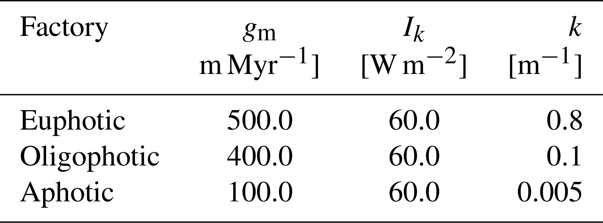
In the examples presented here we set default values of factory parameters that corrspond to three biological facies based on sediment produced by three carbonate factories: the euphotic (E), oligophotic (O) and aphotic (A) factories. These default values are shown in Table 1, and the resulting production curves shown in Fig. 1.

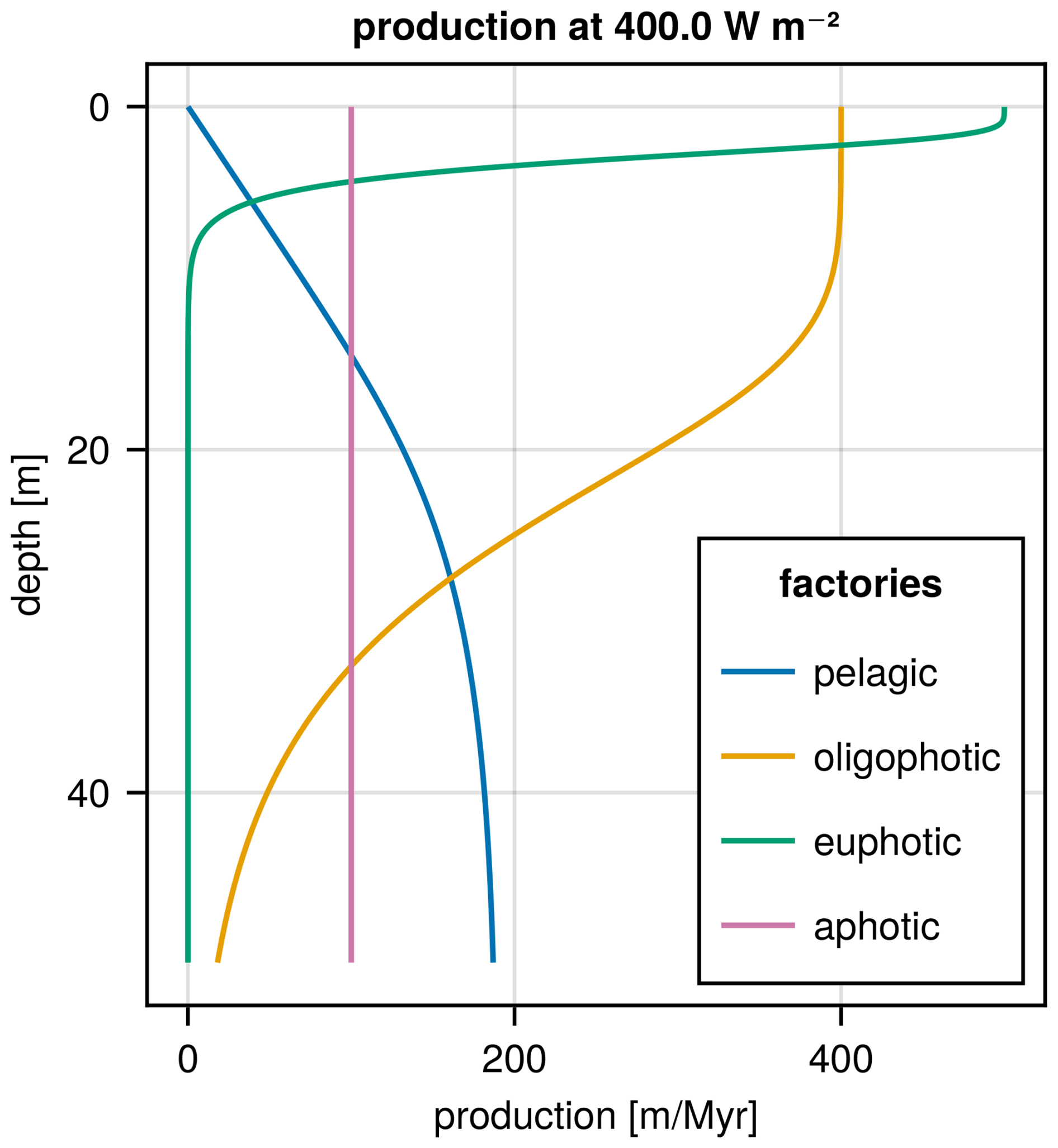
Figure 1 Production curves for our three default carbonate factories. Additionaly, we show the production curve for a pelagic facies with the same extinction coefficient and saturation intensity as the oligophotic facies, and a maximum growth rate of 5 Myr⁻¹. All of these production curves were computed with an insolation of 400 W m⁻².

Table 1 Parameters for the production model of the three default carbonate factories.

We also provide the option of specifying pelagic production curves. Here the production is computed as the integral of Eq. (3) over the entire water column.

2.3 Cellular automaton

Representing spatial heterogeneity resulting from positive and negative biological interactions in a computationally simple model requires meeting the following conditions:

1. infinite heterogeneity in space and time, i.e. no convergence on stable patterns;

2. authigenic variation that does not require external drivers;

3. the approach must be scalable to n facies, even if we focus the examples here on 3;

4. adjustable temporal persistence: it must be possible to set the turnover frequency.

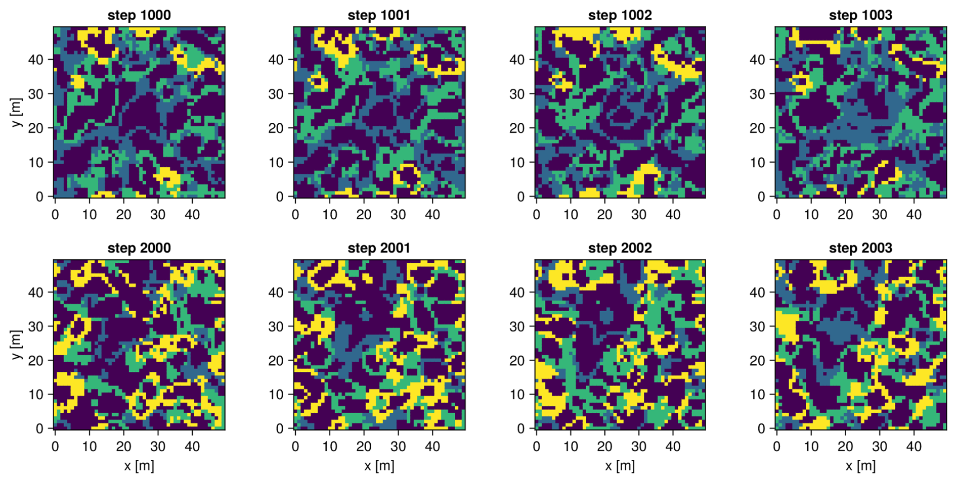
Figure 2 Iterations of the CA, as described by Burgess (2013), on a periodic grid of 50×50. Each color represents a carbonate facies, but since the CA process is not affected by facies identity we leave out any designation. Starting with random noise, we first iterate 1000 times to get into a typical state. The top row shows iterations 1000 to 1003, the bottom row 2000 to 2003. This shows that the patterns keep reasonably stable on the short term, while evolving more extensively over the long term.

These requirements are met by Celullar Automata (CA), as proposed by Drummond and Dugan (1999), Burgess and Emery (2004) and Burgess (2013), without substanial computational costs. For this reason we adopt this modeling approach in CarboKitten, directly reimplementing the automaton described by Burgess (2013) in his package CarboCAT. Cellular automata are commonly used to generate spatial heterogeneity in forward modeling, with some models serving as discrete approximations of partial differential equations that can generate complex spatial dynamics such as Turing patterns (Drummond and Dugan, 1999; Dormann et al., 2001).

The CA emulates the biological succession of species by following a set of simple rules. If conditions are right, a species will multiply and occupy neighbouring territory. However, when there are too many of the same kind, the species will die from over population. For each cell in the grid a centered neighbourhood of 5×5 pixels is considered. We count the number of neighbouring cells of the same species. Then we consider two ranges: the activation range (default $\mathrm{6}\le n\le \mathrm{10}$) and viability range (default $\mathrm{4}\le n\le \mathrm{10}$). If the number of live neighbours is in the viability range, the cell stays alive. If the cell was dead, but the number of live neighbours is in the activation range, the cell becomes alive. The neighborhood size and the rules represent a case of Larger than Life family of two-dimensional cellular automata (Evans, 1996), but this particular set of rules has been proposed specifically for CarboCAT (Burgess, 2013) and, to our knowledge, does not correspond to any documented Larger than Life rules. We examined other sets of rules (Hidding et al., 2026b), but most lead to rapid stabilization of spatial patterns. In Fig. 2 we illustrate the long-term and short-term behaviour of our default CA rule set.

The initial CA grid is randomized. A dead cell may qualify to become alive for different carbonate factories at the same time. To resolve this priority collision, facies priority for occupying a dead cell is rotated every iteration using a deterministic cyclic shift (fixed round-robin pattern), which ensures that there is no priority given to any facies.

In the default configuration we emulate three species, corresponding to the factory species discussed in the section on carbonate production. The state of the CA determines which carbonate factory is switched on for each cell in the grid.

The 5×5 neighborhood strikes a balance between small-scale heterogeneity and computational cost. A smaller neighborhood would result in finer-grained spatial patterns, whereas a larger one in spatial smoothing and larger, more coherent patches of each facies. However, it would slow the model down. In a real depositional system, different carbonate producer guilds have their own length scales at which they disperse and interact and one-size-fits-all neighborhood is clearly a simplification. The size of the neighborhood is fixed in the current version of CarboKitten, but adjustment of granularity of facies distribution generated by the CA can be achieved by users by changing the grid dimensions and the CA interval.

2.4 Transport

Our transport model is borrowed from other similar approaches in siliclastic (river bed) modeling (see Paola et al., 1992; James et al., 2010), where it is made plausible that this approach is viable for models that work on long time scales. Because our transport model is novel (at least for modelling carbonate platforms), we discuss the full model in a separate section. Here, we discuss how transport is embedded in the larger model.

We consider all sediment transport to happen in an active layer close to the sea floor. This layer has a certain amount of sediment C_f (in units of m) that travels along a path of steepest descent. We say that this material is entrained. Every time step the active layer is supplied with sediment produced in the production step as well as older sediment through disintegration. After transport a fraction of the entrained sediment is deposited on the sea floor as the transported version of the original (donor) facies in a process that we refer to as lithification, being the process of turning loose sediment into rock. Although in reality sediment might not be mobile for a while before lithification sets in, for the purpose of our model, we chose the term to represent the immobilisation of sediment as a whole, see Fig. 3.

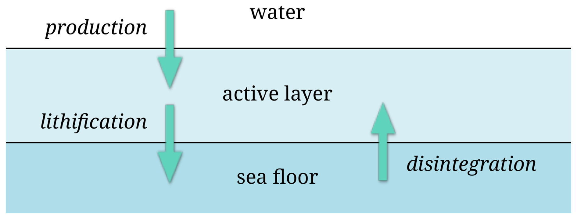
Figure 3 Diagram showing concepts of production, lithification and disintegration. Every time step newly produced sediment and older disintegrated material (configured as a disintegration rate) is added to the active layer. After transport, a set fraction of the sediment (configured as a lithification half-life time) is lithified, becoming the sea floor.

The actual transport is computed using a finite difference approach that is further discussed in Sect. 3.

2.5 Composed model

Putting everything together, we evaluate the model as follows each iteration:

1. Advance the cellular automaton.

2. Compute the production P_f.

3. Disintegrate sediment at the rate r_d.

4. Transport entrained sediment C_f.

5. Lithify (cement) sediment with half-time of t_l.

Advancing the CA can be configured to happen one-in-n iterations to slow it down. Transporting the sediment can be computed on smaller time steps if required for numeric stability. The complete loop is illustrated in Fig. 4.

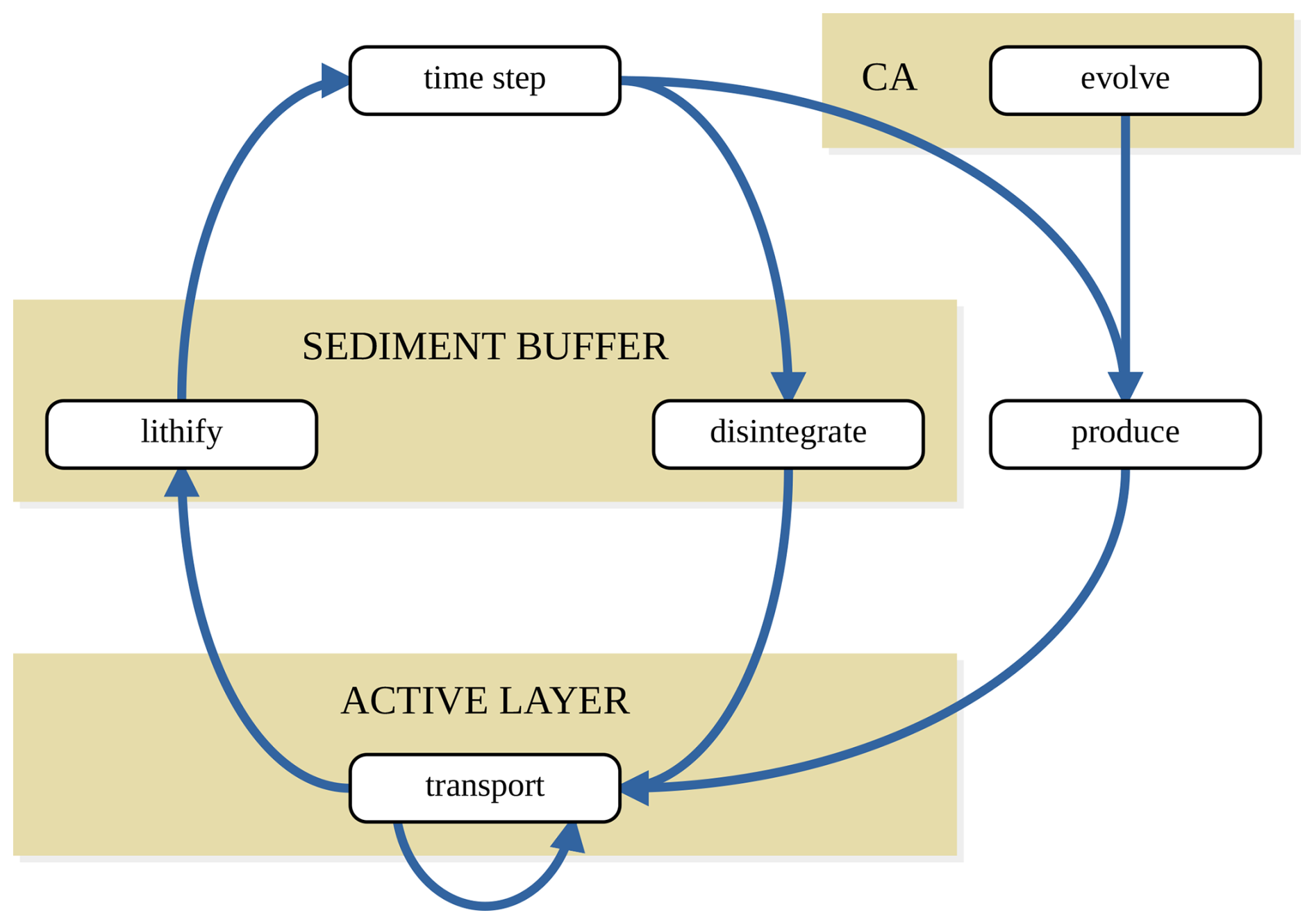
Figure 4 Flow chart of model control. The shaded areas show where the internal states of the CA, sediment buffer and active layer are affected. We can follow the model, starting from the time step node. The time step implies a change in external control factors like sea level, subsidence and insolation. Together with the sediment buffer, those factors determine water depth which in turn affects both production and transport. The CA evolves by itself (there is an option for feedback from the production step, but we left it out of the diagram for simplicity), but determines which facies are produced where. We then produce and disintegrate sediment that is added to the active layer for transport. The transport step is adaptive, so it can loop several times before we lithify a fraction of the active layer. After lithification, we increment the time step, completing the loop.

2.6 Input parameters

CarboKitten has many input parameters: box geometry, time parameters, a list of facies properties, transport model intrinsics and external conditions such as initial topography, relative sea level and insolation. We have already discussed the facies properties in Sect. 2.2, and the transport model is discussed in Sect. 3. That leaves us the external conditions that should be considered the driving forces of carbonate platform formation.

The initial topography, sea level and insolation can all be entered in three different ways: a given constant, a Julia function or an array exactly matching the box size or number of time steps.

In Sect. 6 we provide two examples where we use external sources to drive the sea level and insolation curves. A full list of input parameters is available in the Appendix.

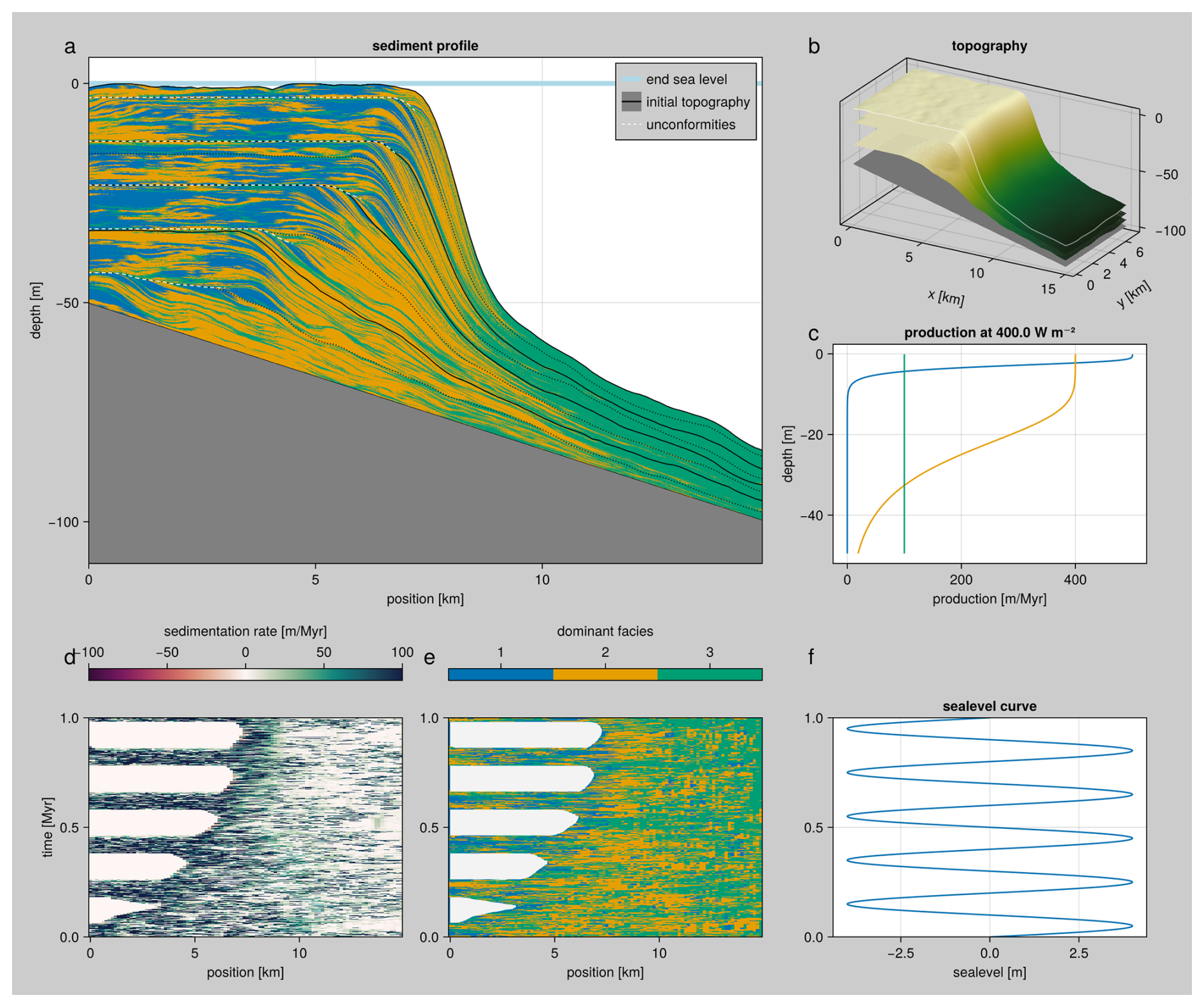
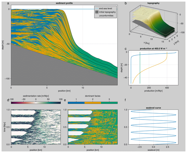
Figure 5 Overview of different visualizations supported by CarboKitten. Panel (a) shows a stratigraphic cross-section, including an indication for unconformities, (b) a topographic overview including two intermediate time steps, (c) the production curves used, (d) sedimentation rate as a function of time, (e) Wheeler diagram with preserved dominant facies as a function of time, (f) the sea-level curve given as input. The combined plot is arranged such that spatial data is on the top row, while time-dependent information is shown at the bottom with matching y axes.

2.7 Visualisations

CarboKitten generates data in the accessible, binary HDF5 format, thus output can be visualised with most common tools, e.g. imported into R or a Jupyter notebook. Nevertheless, we provide some routines based on Makie (Danisch and Krumbiegel, 2021) for creating cross-sections, chronostratigrahic (Wheeler) diagrams and topographic overviews. Some of the most common plot types have been collected into a summary plot, which is shown in Fig. 5.

3 Transport

The transport module is designed with timesteps of the order of centuries in mind and therefore it aims to lead to a similar average sediment redistribution as would have resulted from individual short-term physical processes (storms, waves, tidal currents, grain-size sorting), without attempting to resolve them. CarboKitten currently does not resolve grain-size-dependent transport, storm-driven episodic redistribution, longshore transport, or bioturbation contributing to sediment disintegration. However, such extensions are principally possible, should modelling on shorter time scales become the focus of the model's users.

In Sect. 2.4 we discussed how transport is embedded in the larger model. Our transport model supposes that all entrained sediment resides in a layer of constant thickness just above the sea floor, also known as the active layer. The concentration of sediment C_f (in units of m) is considered separately for each facies (as with all quantities with the “f” subscript). Each iteration of the larger model we supply the active layer with freshly produced (autochthonous) sediment as well as disintegrated older (allochthonous) sediment. We then compute transport of the active layer for as many sub-iterations as is deemed needed for the solver to remain stable. After that, a percentage of the contents in the active layer is deposited on the sea floor. The lithification percentage depends both on the time step taken and the given lithification time t_l, which is configured in terms of a half-life time. There are many ways to compute sediment transport in the active layer. We have opted for a finite difference strategy inspired by Paola et al. (1992).

We assume a local sediment flux proportional to the local gradient,

$$\begin{array}{}\text{(5)}& {\mathit{q}}_{\mathrm{f}}=-C_{\mathrm{f}}{d}_{\mathrm{f}}\mathbf{\nabla }\mathit{\eta }+C_{\mathrm{f}}{\mathit{v}}_{\mathrm{f}}\left(w\right)\end{array}$$

where d_f is a facies-dependent transport coefficient (m Myr⁻¹), and v_f(w) is a chosen additional velocity as a function of water depth (m Myr⁻¹). Optionally, we use v_f(w) to model wave induced sediment transport (for an example see Sect. 6.3). The mass balance (continuity equation) is then,

$$\begin{array}{}\text{(6)}& {\displaystyle \frac{\partial C_{\mathrm{f}}}{\partial t}}=-\mathbf{\nabla }\cdot {\mathit{q}}_{\mathrm{f}}.\end{array}$$

This gives us an advection equation for the sediment concentration C_f. We also express everything in terms of water depth, having $\mathrm{\nabla }w=-\mathrm{\nabla }\mathit{\eta }$, arriving at

$$\begin{array}{}\text{(7)}& {\displaystyle \frac{\partial C_{\mathrm{f}}}{\partial t}}=-\left(d_{\mathrm{f}}\mathbf{\nabla }w+{\mathit{v}}_{\mathrm{f}}\left(w\right)\right)\cdot \mathbf{\nabla }{C}_{\mathrm{f}}-\left(d_{\mathrm{f}}{\mathrm{\nabla }}^{\mathrm{2}}w+{\mathit{s}}_{\mathrm{f}}\left(w\right)\cdot \mathbf{\nabla }w\right)C_{\mathrm{f}},\end{array}$$

where ${\mathit{s}}_{\mathrm{f}}\left(w\right)={\mathit{v}}_{\mathrm{f}}^{\prime }\left(w\right)$ is the velocity shear, or the derivative of the velocity with respect to water depth. We solve this PDE using a finite difference method-of-lines approach with an explicit solver (forward Euler and 4th order Runge–Kuta are supported).

Note that, although the transport equation is an advection equation in C_f, we need to consider that C_f acts as a proxy for η. The continuing cycle of disintegration, transport, and lithification makes sure that the change in sediment concentration due to transport and the change in topography are strongly coupled. Then, what seems like an innocent reaction term in Eq. (7), turns out to behave as a diffusion equation in η. Any attempt at modelling sediment transport where there is an effective down-slope flux combined with some form of disintegration will yield diffusive behaviour.

3.1 Other approaches

In the critical angle approach developed by Warrlich (2000), sediment is transported from unstable slopes to the nearest down-slope stable region. Stability is defined separately for different grain sizes. This method is motivated by the empirical relationship between grain composition and maximum slope angle (Kenter, 1990).

The problem with this critical angle-based method of transport is that production across an unstable region is deposited on a small strip, where slopes are below the critical angle. It becomes unclear how to interpret these models from a physics point of view, as results depend heavily on the time-step that is chosen. Contrasting to that, both our transport model and production model (with the exception of the cellular automaton) are discretisations of otherwise continuous processes. This means that, at least assymptotically (i.e. as long as the time step is small enough), our implementation is independent of the chosen time step.

One aspect of critical angle theory that we do use is that we can modulate the disintegration rate r_d (and therefore the amount of entrained material) with the magnitude of the slope $\left|\mathrm{\nabla }\mathit{\eta }\right|$. If we only disintegrate material where the slope is supercritical, the net effect is that sediment is transported from supercritical to stable areas. The difference is that we have a much better control over the physics, and there is no need to convert back and forth between gridded values and a particle representation used in the critical angle approach (e.g. Warrlich, 2000). A different approach has been used in the early model CARBPLAT by Bosscher and Southam (1992), which took empirically observed carbonate slopes (Kenter, 1990, Adams and Schlager (2000)) and defined a slope function that returned slope parameters bounded by the limits of the angle of repose. In the study by Bosscher and Southam (1992) an exponential slope function was assumed, although it should be noted that there is literature debate on the distribution of slope shapes of carbonate platforms (e.g., Schlager and Camber, 1986; Kenter, 1990; Adams and Schlager, 2000). This modelling approach is agnostic with respect to sediment properties and transport mechanisms and optimises the similarity to observed shapes, allowing the user to choose the parameter that produces the best result. However, it does not allow modelling a mixture of sediment types with different properties and requires an a priori assumption on the expected slope shape. It had not been adapted in subsequent models.

3.2 Parameter choices

Our transport model is based on the elementary assumption that sediment flux is proportional to the slope of the sea floor. Nevertheless, we are extrapolating this idea to time scales on which it is hard to reason or otherwise measure the parameters to our model. Especially the combination of transport coefficient d_f, disintegration rate r_d and lithification time t_l can be pivotal in acquiring a set of physical outcomes, while we have no good way to estimate acceptable ranges of values for them, other than trying them out and see if the results are plausible.

That being said, by considering some artificial scenarios we can gain more insight into the behaviour of our main parameters.

3.2.1 Disintegration versus subsidence

The chosen disintegration rate will determine whether our model is on average erosive or accumulative. In the case of a platform morphology, the potential production exceeds the subsidence, meaning that the subsidence rate sets the pace at which the platform grows. At the edge of the platform, there is a transitional region where the maximum production is at pace with the subsidence. If the distintegration rate is higher than the subsidence rate, produced sediment will be immediately disintegrated, stay in the active layer for much longer, and be transported down slope. If the disintegration rate is much lower than the subsidence rate, produced (autochthonous) sediment can accumulate in situ, generating steeper morphologies.

3.2.2 Equilibrium concentration

The model parametrizes sediment disintegration (i.e. activation or entrainment of older sediments) by a global constant disintegration rate r_d. Entrained sediment is transported by the mechanism described above, and then (re)lithifies by a given percentage every time step. The lithification time is specified as a half-life time t_l. In absence of production, and with infinite available sediment for disintegration, we can see the amount of entrained sediment C reaching an equilibrium:

$$\begin{array}{}\text{(8)}& C(t+\mathrm{\Delta }t)=C\left(t\right){\mathrm{2}}^{-\mathrm{\Delta }t/t_{\mathrm{l}}}+r\mathrm{\Delta }t,\end{array}$$

and taking the limit Δt→0, the equilibrium is reached at,

$$\begin{array}{}\text{(9)}& \langle C\rangle ={\displaystyle \frac{\mathrm{1}}{\ln \mathrm{2}}}{r}_{\mathrm{d}}{t}_{\mathrm{l}}.\end{array}$$

This equilibrium (having units of m) can be useful when estimating the effects of choosing the disintegration rate and lithification time.

3.2.3 Disintegration versus lithification

Both the disintegration rate and the lithification time modulate how long sediment resides in the active layer. By carefully scaling one or the other, the effective diffusion of material can be controlled without changing the specific diffusivity. However, choosing a high lithification time (thus a slow lithification) over a high disintegration rate can help in transporting only freshly produced sediments.

Note that not setting the lithification time (which would amount to immediately depositing all of the active layer on every iteration) results in models that depend heavily on a chosen time step.

To understand the relative effects of choosing a certain lithification time and/or disintegration rate, we ran a one-dimensional model where sediment is produced in a central patch. Then we can study the rate at which sediment is dispersed, either by direct transport before lithification happens, or by subsequent disintegration and re-deposition. By carefully choosing the parameters, we can make a slow lithification process look very similar to a high disintegration rate, as shown in Fig. 6.

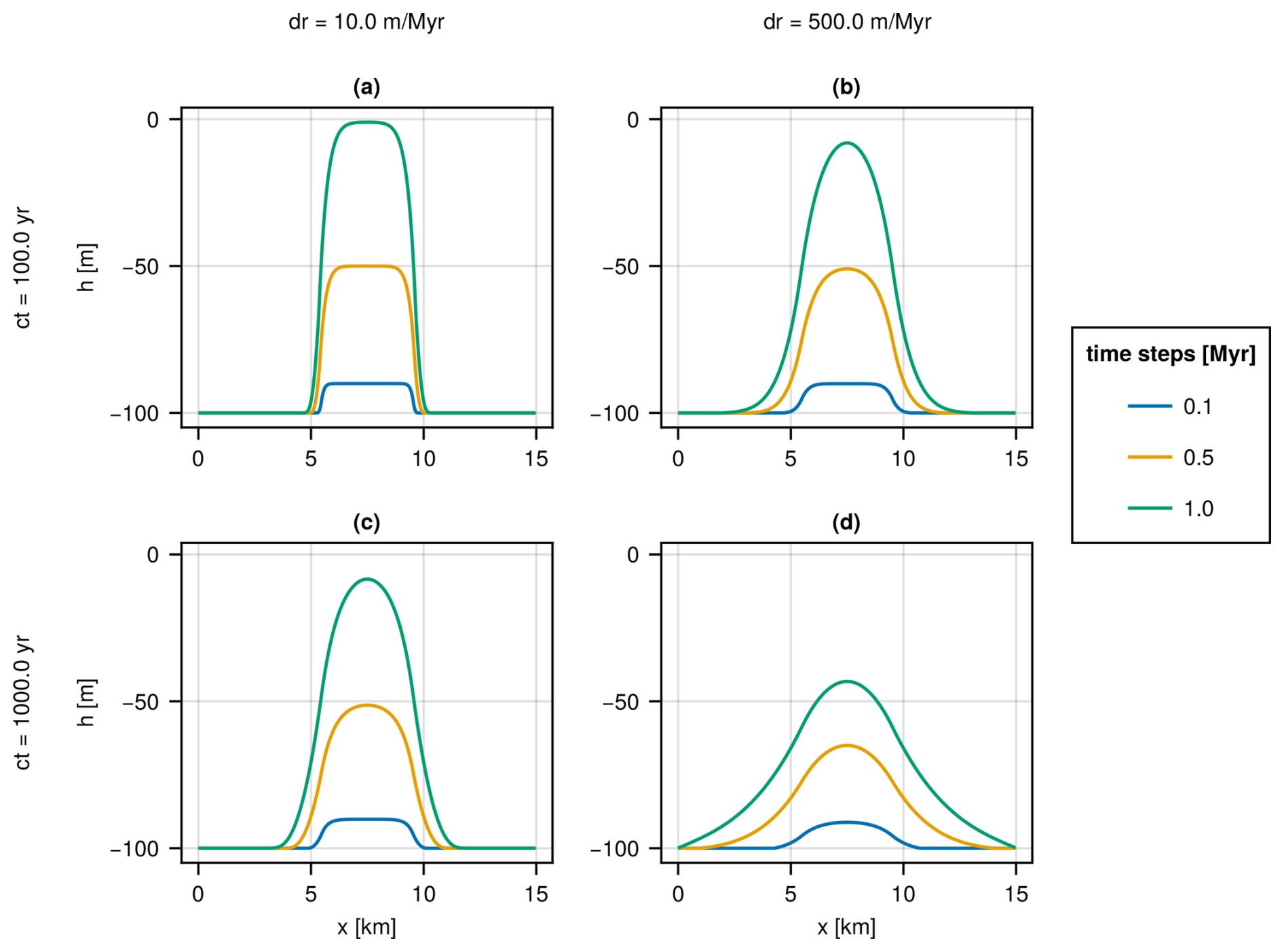
Figure 6 Comparison between lithification and disintegration. The four panes show different combinations of parameters for a one-dimensional model. We have enabled a production of 100 m Myr⁻¹ for a 4 km wide patch in the middle of the box, and chose a runtime of 1 Myr with a time step of 100 year (the sharp edges in the production profile induce fast transport, requiring small time steps), and the transport coefficient was set to 10 m Myr⁻¹. Panels (a) and (b) have a short lithification time t_l (100 year), while panels (c) and (d) have a long lithification time (1000 year). On the columns, (a) and (c) have a low disintegration rate r_d (10 m Myr⁻¹), while (b) and (d) have a high disintegration rate (500 m Myr⁻¹). Values were chosen to have a similar net effect on the dispersion of produced sediment.

3.2.4 Facies-specific transport coefficient d_f

The facies-specific transport coefficient used in CarboKitten is expressed in m Myr⁻¹, because it is derived from the parameter ν_f, transport velocity, that is expressed per unit slope. A diffusion coefficient d_f appears in ${\partial }_t\mathit{\eta }=d_{\mathrm{f}}{\mathrm{\nabla }}^{\mathrm{2}}\mathit{\eta }$ and have units m² Myr⁻¹. In CarboKitten's formulation ν_f is one dimension of length smaller because the active-layer concentration C_f [m] is already present in the flux. This approach presents two challenges: (1) setting transport coefficients that yield realistic results for carbonate facies modeled at the timescales at which CarboKitten is run, (2) should empirically justified diffusion coefficients for carbonate sediment be available, converting these diffusion coefficients to values of the transport coefficient used in the model. Because advection-diffusion is a modeling approach in carbonate transport and not a direct representation of the physical process of sediment transport, prior empirical diffusion coefficient values are limited. Sultana et al. (2022) reviewed published values, which lie in the range of 10⁵ m² Myr⁻¹ to 7×10⁹ m² Myr⁻¹ (Bosence et al., 1994; Mitchell et al., 1996). Modeling studies differ on the orders of magnitude, which is partly a matter of what processes are accounted for in effective diffusivity, and partly reflects different timescales of measurement. In Dionisos simulations, Sultana et al. (2022) used values ranging from 1.25×10⁶ m² Myr⁻¹ for the sand fraction in the photozoan factory to 50×10⁶ m² Myr⁻¹ for the mud produced by the heterozoan factory and identified 2500 10⁵ m² Myr⁻¹ as the upper limit, beyond which no sediment accumulation took place. In a different model, values many orders of magnitude lower have been proposed for the effective diffusion coefficient that implicitly accounts for lithification and depth-dependent wave velocity, introduced by Kaufman et al. (1991):

$$\begin{array}{}\text{(10)}& D_{\mathrm{Kaufman}}\left(W\right)=C_{\mathrm{0}}\exp \left(-C_W\right)\end{array}$$

where C₀=0.005 m² Myr⁻¹ for carbonates and C₁ values considered are 0.05 and 0.1 m⁻¹, resulting in maximum D_Kaufman values of 0.005 m² Myr⁻¹, i.e. much lower than the empirical ones.

Table 2 Estimated effective diffusivity D_eff (m² Myr⁻¹) for combinations of lithification time t_l and disintegration rate r_d at facies transport coefficient d_f equal to 5 m yr⁻¹.

Effective sediment diffusion coefficient D_eff values in CarboKitten runs can be estimated from the dispersal of a sediment pulse under any scenario with a given value of transport coefficient, lithification time and disintegration rate. Diffusivity values obtained from runs with a transport coefficient of 5 m Myr⁻¹ lie in the range of 3.7×10⁵ m² Myr⁻¹ to 8.8×10⁶ m² Myr⁻¹ (Table 2), i.e. well within those reported empirically and overlapping with those used by Sultana et al. (2022) to obtain realistic platform morphologies. Effective D_eff values obtained using this estimate scale linearly with the input transport coefficient d_f.

3.3 Implementation and limitations

Our implementation of the transport model first computes the gradient of the sea floor (or equivalently the water depth) ∇w using central differences. From this gradient we can compute the advection coefficients in Eq. (7), ${\mathit{c}}_{\mathrm{adv}}=d_{\mathrm{f}}\mathbf{\nabla }\mathit{\eta }+{\mathit{v}}_{\mathrm{f}}\left(w\right)$. The maximum advection coefficient sets the Courant number and determines how many time steps we need to take to solve Eq. (7). For an advection equation integrated with the forward Euler method, we need

$$\begin{array}{}\text{(11)}& |c_{\mathrm{adv}}{|}_{\mathrm{\infty }}{\displaystyle \frac{\mathrm{\Delta }t}{\mathrm{\Delta }x}}\le \mathrm{1}.\end{array}$$

This states that we cannot move matter further than a single pixel distance in one iteration, or our computation becomes unstable.

In practice, we compute the transport coefficients and the maximum resulting advective Courant number. Then we integrate the transport equation adaptively, choosing the minimum number of subdivided time steps that keeps the advection stable. Since we computed the transport coefficients in advance, it is relatively cheap to apply multiple iterations of the advection solver, for which we use a first-order upwind scheme.

Now consider our transport model in the context of the larger carbonate platform model. Each time we disintegrate some matter which gets entrained and transported as part of the sediment concentration C_f, after which a fraction is cemented, increasing η. If we consider $\partial \mathit{\eta }/\partial t\sim \partial C/\partial t$, then part of the transport equation is the diffusion equation $\partial \mathit{\eta }/\partial t\sim d_{\mathrm{f}}{C}_{\mathrm{f}}{\mathrm{\nabla }}^{\mathrm{2}}\mathit{\eta }$. This leaves our implementation vulnerable to instabilities when the global time step is taken too large. For just this diffusion term the CFL limit is

$$\begin{array}{}\text{(12)}& d_{\mathrm{f}}{C}_{\mathrm{f}}{\displaystyle \frac{\mathrm{\Delta }t}{(\mathrm{\Delta }x{)}^{\mathrm{2}}}}\le \mathrm{1}.\end{array}$$

This means that increasing the resolution of a model by a factor two may need a time step four times smaller for the integration to remain stable. CarboKitten has a diagnostic mode where this condition is checked against, allowing the user to make informed changes to the input parameters. Because the sediment concentration is not known in advance, it is not possible to make this check in advance.

4 Validation

We validated the model by attempting to replicate the general architecture of an isolated carbonate platform in Central Luconia (part of the Sarawak Basin), offshore Malaysia (Cycle IV to Cycle Lower V). We chose this area is because this platform has been extensively studied (Henglai et al., 2024) and the interpreted seismic profiles and reconstructed sea-level curves were publicly reported. We informed model runs with the sea-level data obtained from Fig. 2 of Henglai et al. (2024). In addition, the tectonic setting of the region in the studied period (around 15.48 to 11 Ma) is believed to be uncomplicated (Fathiyah Jamaludin, 2025) and thus possible to represent with a constant subsidence rate. Four wells were drilled into the atoll, providing discontinous cores and, thus, geological facies information.

This platform has a pinnacle shape, with the length of approximately 5 km in NE–SW direction, suggesting it was drowned in during this time period. The cores indicate that the top of carbonate platform is dominated by coral boundstones. Although the sampling in the lower part of the cores is discontinous, the cores suggest that the facies are dominated by pack- to wackestones and interbeded by coral boundstones, bioclastic boundstones and argillaceous carbonate. We related the geological facies to the carbonate producers via Table 3.

Table 3 Facies used in validation. We used three producing facies in modelling our validation case, and a fourth facies type to track transported coral.

n/a means not applicable.

Three carbonate producers are fed into the model, corresponding to three geological facies (producers). Their respective production rates are listed in Table 3. A fourth facies is the transported facies of euphotic corals. These values are within the production rates estimated by (Lopez-Gamundi et al., 2025). A pre-run was set in order to generate an atoll-like initial topography for the actual run. The total duration of modelling covers the entire Cycle IV (from 15.8 to 11.8 Ma, having a duration of 4 Myr).

The criteria for comparison between the modelled results and the interpreted seismic profiles were:

1. We obtain five major zones within the platform.

2. The platform should show a pinnacle shape.

3. The total thickness of carbonate stratigraphy is approximately (600 m).

4. The platform has a slope indicating presence of off-shore sediments transport.

The results are listed in Fig. 7. We compared the features in the figure and the interpreted seimic profile:

1. The interpreted seismic profiles suggested five zones, and this is captured in the resultant figure (five parasequences).

2. The results displayed a “pinacle” shape, showing upper parasequences bearing smaller horizonal dimensions than the lower parasequences.

3. The total thickness of carbonate (∼550 m) is comparable to the data suggested by well penetration (∼600 m).

4. The slope is presented in the modelled results, as a mixture of facies 3 and 4.

The model yields nearly identical – i.e., qualitatively the same – results for different timesteps. Users should note that changing the timestep requires adjusting the CA interval, which has been applied for the tested versions of the code: a timestep of 100, 250 and 250 year. Results for a time step of 400 year are shown in Fig. 7.

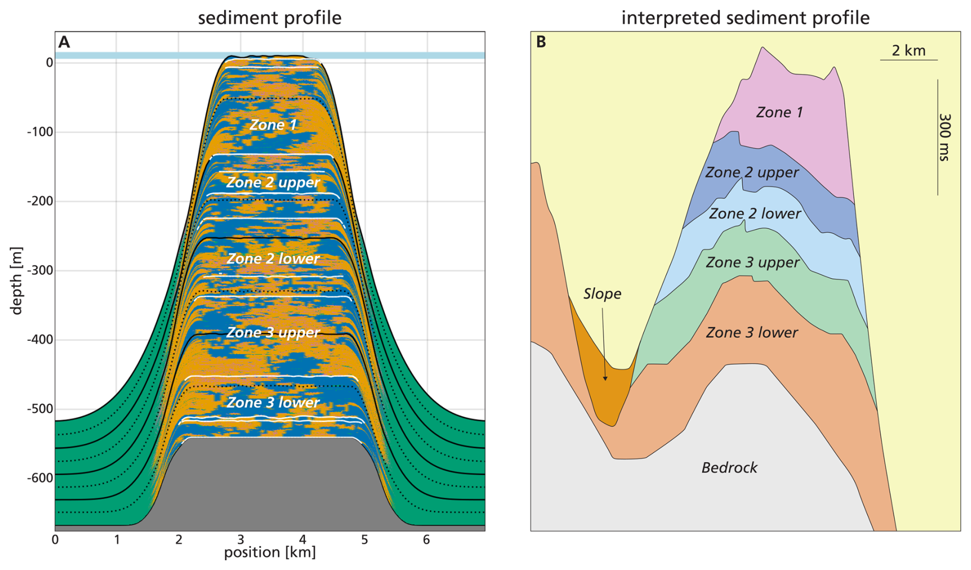
Figure 7 Validation case. (A) This shows a cross-section of our model of the platform in Central Luconia, offshore Malaysia. The white lines indicate unconformities, and the black lines are coeval lines at regular intervals, every solid black line separating one million years. The colours indicate the dominant facies type of the modelled sediment, blue for facies 1 (T factory), yellow for facies 2 (M factory), green for facies 3 (P factory) and pink represents facies 4 (transported coral, i.e. formerly facies 1). (B) Seismic interpretation of the platform, redrawn from Fig. 9 of Henglai et al. (2024).

Therefore, we claim CarboKitten is able to reproduce major architectural features of a real-life carbonate platform.

5 Software design

5.1 Box topology

CarboKitten needs to work with different choices for box topology, i.e. how the boundaries of a model box connect to each other. For example, when we simulate a small strip of coastline it is best to have one axis (in this case the x axis) reflect onto itself, while the other axis is periodic, leaving fewer edge effects.

In another case, where we want to simulate an entire island, or even an archipelago, it is more convenient to use fully periodic coordinates. We illustrate these choices in Fig. 8.

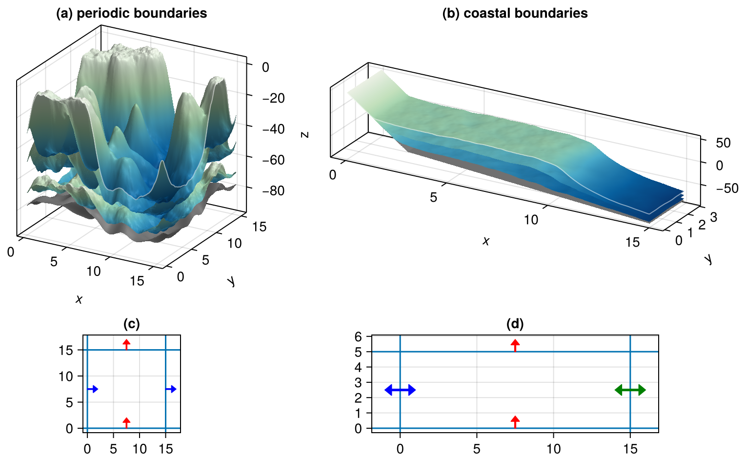
Figure 8 Model topologies. CarboKitten allows the user to choose different topologies for the spatial modelling. In panel (a) we see a group of reef islands that were modelled on a fully periodic grid of size 250×250, using a randomly generated initial topography. A more common use case is shown in panel (b), where the x coordinate is reflected at the boundaries, while the y coordinate is periodic, thus modelling a small strip of coastline. Here the grid size is 250×50, and the initial topography is a linearly declining slope of 0.3 % (with the exception of the shore, which is steeper). The superimposed surfaces represent different equidistant time steps in the same runs, while the colors indicate the elevation along with the values on the z axis, here provided to guide the viewer. Panels (c) and (d) schematically illustrate these same box topologies using coloured arrows.

5.2 The sediment buffer

In our models of sediment transport and denudation it is important to remember the sedimentation history for all produced facies for some time into the past. We keep a three-dimensional fixed-size buffer, where two dimensions represent the x and y coordinates of the system, and the third dimension discretizes the amount of deposited material. Each cell in the buffer represents a parcel of sediment, where we store the relative fractions of each contributing facies. The data-structure acts like a stack, working on a First-In-First-Out (FIFO) basis.

We emphasise that this buffer is only used to determine the facies composition of disintegrated sediment. The sediment output of the overall model is written to disk at each iteration for post-analysis. This means that the model output can be much more precise than the depositional resolution of the buffer.

The user can set the size of the buffer as well as the amount of sediment represented by each cell. The depth of the buffer is controlled by an input parameter sediment_buffer_size, while the resolution is set through the depositional_resolution parameter in units of m of sediment.

The rows in the buffer represent a constant amount of sediment. An alternative approach is to have rows that represent time slices. In that case, when we need to disintegrate an amount of sediment, we need to search the buffer back in time until enough sediment is collected. This can be very slow, and it also means that one needs to have the full sedimentation history in memory. A buffer that is discretized on depth however does not have those requirements, at the expense of a small amount of facies mixing.

While the sediment buffer is allocated as a single 4-dimensional array (depth, facies, x, y), it is best to explain its functioning from the perspective of a single cell in our model. We are left with two dimensions: depth (rows) and facies (columns).

We choose to have the head of our sediment stack always be at the first row. When sediment out-grows the buffer, the deepest layers are dropped from memory. The head can contain an incomplete amount of sediment, while all rows below the head are either full or empty. When sediment is pushed to the stack and the head row overflows, all rows are copied down one row and the surplus is assigned to the now empty head row. The inverse happens when removing (popping) material from the stack. This process is illustrated below in Fig. 9.

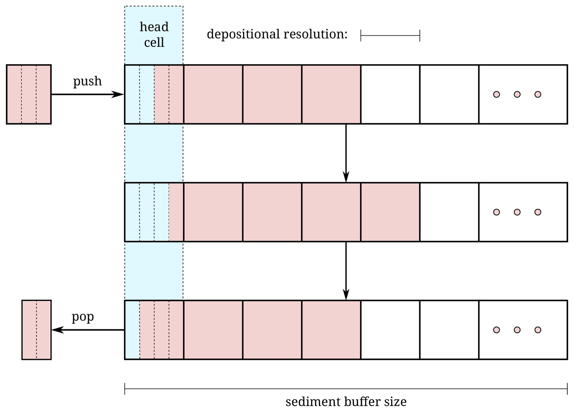
Figure 9 Above we see a buffer. Suppose we first produce some sediment amounting to $\mathrm{3}/\mathrm{4}$ of the buffer resolution, and after that an amount of $\mathrm{1}/\mathrm{2}$ gets disintegrated for further transport. In the beginning, the top cell of our buffer is $\mathrm{1}/\mathrm{2}$ full. First we push a parcel of (relative) size $\mathrm{3}/\mathrm{4}$. The remaining $\mathrm{1}/\mathrm{4}$ overflows to the next cell. Then we pop an amount of $\mathrm{1}/\mathrm{2}$. The first $\mathrm{1}/\mathrm{4}$ of this amount is retrieved from the top cell, and the second $\mathrm{1}/\mathrm{4}$ from the cell below that. This popped parcel will have different fractions from the pushed one, since it also draws from the half filled row that was in the stack before pushing. In this sense, a small amount of facies mixing will take place, depending on the depositional resolution chosen.

5.3 User interface

The user interfaces CarboKitten by writing a Julia script that defines the relevant model parameters and runs the chosen model. Effectively, very little Julia needs to be known to take an example input and modify parameters. Output is written to HDF5 files for post-processing and visualization.

CarboKitten ships with routines for visualisation and data extraction into CSV files. This makes it easier for novice users to use results from CarboKitten in further processing pipelines that rely on other programming languages. Data extracted includes sediment accumulation curves, age-depth models, water depth, and stratigraphic columns with facies code, allowing to test a wide range of hypotheses. These include, but are not limited to, testing hypotheses on orderedness of strata (Burgess, 2016), preservation orbital forcing (Kemp et al., 2016), proxy records (Curtis et al., 2025), or preservation of biotic information such as patterns of origination and extinction, biostratigraphic precision, and evolutionary change (Hohmann and Jarochowska, 2025; Hohmann et al., 2024; Holland and Patzkowsky, 2002).

5.4 Performance

Since CarboKitten is written in Julia with performance in mind, it should be efficient to run, even on consumer grade hardware, i.e. an average laptop. We are yet to substantiate this claim. Since Julia is a just-in-time compiled language, the first execution of any code in a new session always takes a bit longer than subsequent runs. Measurements presented in this section do not include this initial overhead.

5.4.1 Baseline

Our baseline model is the example included in CarboKitten, grid size 100×50 with 5000 time steps of 200 years each (results shown in Fig. 5). This model runs in 27 s on a Intel Core i7 at 3.0 GHz.

With regards to memory consumption, CarboKitten allocates a fixed amount of memory at the start of a model run, which scales linearly with the size of the grid. The most significant fraction of the memory is occupied by the sediment buffer. In the example run we have a buffer size of 50. With three facies types being stored this results in an array size of $\mathrm{100}\times \mathrm{50}\times \mathrm{50}\times \mathrm{3}$, stored in double precision gives a mere 6 MB. However, for a 300×300 sized grid this already increases to 108 MB.

5.4.2 Scaling

The run-time and memory consumption of CarboKitten should scale linearly with the number of pixels in the grid, with two complicating factors. Firstly, for smaller models the run-time can become limited by many smaller writes to HDF5. For those cases we provide a method of running models entirely in-memory. The second complication is the transport model. Here run times may vary due to the number of integration steps required for stability reasons. Increasing the resolution of a model also means increasing the number of transport integration time steps required by the same factor (considering the CFL condition for advective transport). Transport efficiency is also affected by the local topography: increasing the slope also increases the number of integration steps required. Carbonate platforms have the tendency to generate steep slopes due to exponential sedimentation rates in the production model. These steep slopes can be mitigated by setting the transport coefficient d_f: higher values will lead to smoothed-out and gentler slopes. On the other hand, modelling on-shore transport due to wave transport can induce steeper slopes, again requiring smaller integration time steps. Note that we are speaking of integration steps of the transport model, which can be any integer fraction of a full model time step. When the transport model needs too many steps for every model step, we can start to question the accuracy of the model as a whole, and the user should try decreasing the time-step of the full model to compensate.

5.4.3 Benchmark

To further quantify these complications in our estimated run-times, we run a model of a single atoll at three resolutions (200, 100, and 50 m, corresponding to grid sizes of 75², 150², 300²) with three step sizes (400, 200, and 100 years), corresponding to 2500, 5000, and 10 000 steps), for a total of nine benchmark cases. We set the interval of the cellular automaton to compensate for the number of time steps. This way, runs with the same grid size should have very similar output. The results are shown in Fig. 10.

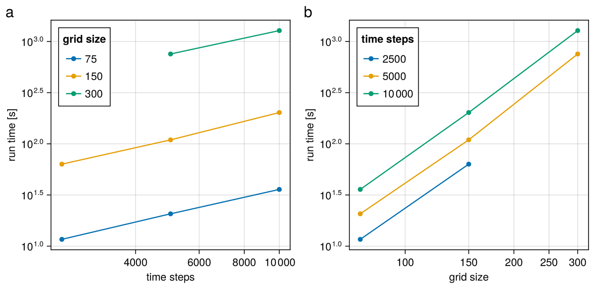
Figure 10 Benchmark with respect to number of time steps and grid size. Panel (a) shows the run-time dependency on the number of time-steps, while panel (b) shows the dependency on the number of grid cells on each axis, both on a log–log scale. This scaling follows the predicted behaviour: linear in both the number of time-steps and total number of grid cells (on this plot being the grid size squared). Note that the run with 2500 time steps and 300² grid size is left out, since the transport model was unstable for that configuration. These numbers were consistent throughout multiple runs.

The combination of 2500 time steps with a 300² grid size yields instabilities in the transport model and is left out of the results. Other than that, CarboKitten scaled as predicted from our previous considerations.

5.4.4 Validation

We may validate our benchmark by looking at the results of the runs with grid size 150². This is shown in Fig. 11. These results show that, when time steps are taken small enough, CarboKitten converges to a consistent result that does not depend on the size of the time step.

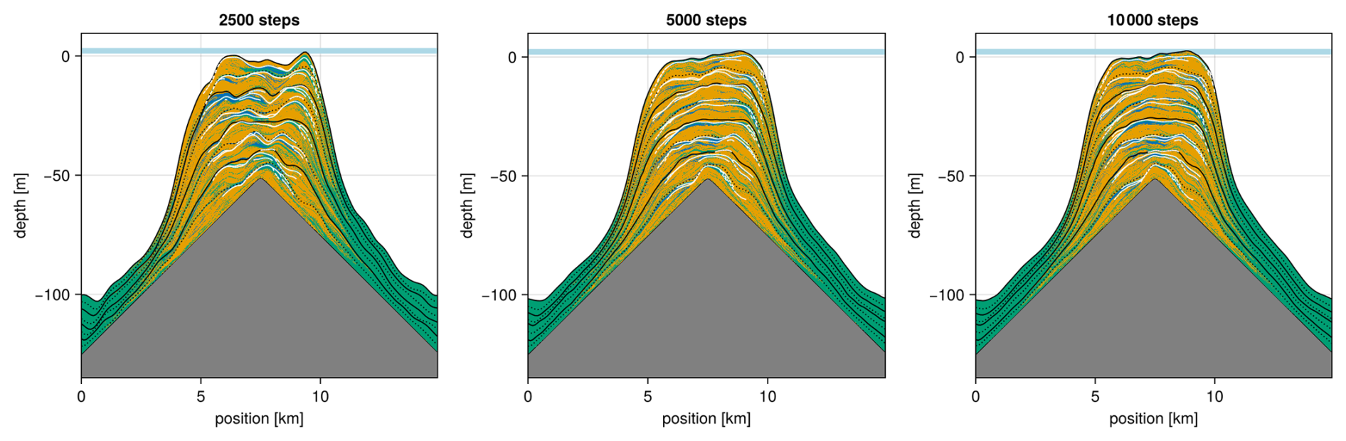
Figure 11 Benchmark validation. This shows a cross-section of the runs with a grid size of 150². Looking at the first output, using only 2500 time steps, we see a wave like pattern even where the deep sea facies dominate. These waves are not physical, but a result from taking the time step too large. When we look at the results from 5000 and 10 000 time steps, they look so similar that we can conclude that in this case 5000 steps was enough to get accurate results.

5.4.5 Potential for GPU optimisation

At the time of writing, CarboKitten is a single threaded CPU code. However, the structure of the model, is highly ammenable to optimisation on a GPU, which would drastically improve run-times further. Going through the steps of the composed model in Sect. 2.5: the cellular automaton is a stencil operation, production a map, disintegration a stencil, transport is implemented as an iterated stencil, and deposition is a map. Both stencil and map operations are highly localized in memory and are ideal for implementation on a GPU.

5.5 Documentation

CarboKitten is written entirely using literate programming (Knuth, 1984). This means that the implementation of CarboKitten is written as an integral part of its own documentation, using a system called Entangled (Hidding, 2023). The aim is that interested readers have a direct reference to the code implementing the methods that are explained in the documentation.

6 Examples

We provide two examples of typical tasks users are likely to undertake: creating a simulation using an empirical, externally provided sea level curve and one with explicit forcing by an insolation curve. These examples are supported by the code used to generate this executable manuscript (FIXME ref to the code) and users are encourage to use that code as a starting point for modifying these examples for their needs.

The third example serves to illustrate the details of how the wave-induced transport is modelled and how modelling decisions and parameter choices affect the outcomes obtained using this feature.

6.1 Sea level

Variables external to the model, which modulate the output the most, are the sea level and insolation. The sea level, together with subsidence, result in the relative sea level, which translates into water depth at any given position in the basin. The sea level must be specified as a function of time. It can be a constant, a continuous function or an empirical dataset. Empirical datasets can be read in as text files and need to be interpolated to equidistant intervals corresponding to the time step with which the model is run. The example here uses the sea level curve by Lisiecki and Raymo (2005), reproduced in the compilation by Miller et al. (2005). The dataset of relative sea level records derived from foraminifer δ¹⁸O extracted from this compilation is included in CarboKitten to facilitate simulations of the most typical sea-level scenarios. In this example we start the model at 2 Ma and build the platform until 134.54 ka, i.e. until the end of the record by Lisiecki and Raymo (2005), using a time step of 200 year (Fig. 12).

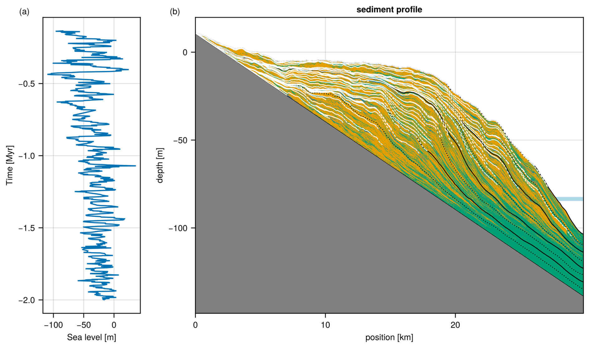
Figure 12 Platform generated using the sea level curve of Lisiecki and Raymo (2005). Panel (a) shows the sea level curve. Panel (b) thecorresponding output stratigraphy.

6.2 Insolation

The relationship between production and insolation can be modified with user-provided parameters. It may be confusing that the extinction coefficient k is, in CarboKitten, a property of the carbonate factory and the facies it deposits and not of the basin or position in it. In reality extinction coefficient varies for different wavelengths of the sunlight spectrum, but the set of its values across the spectrum is constant for a given water body. While different carbonate factories exploit (or ignore, in the case of the aphotic factory) different parts of the light spectrum, the model is agnostic to it and allows users to set k to values that may represent an average across different producers using different wavelengths.

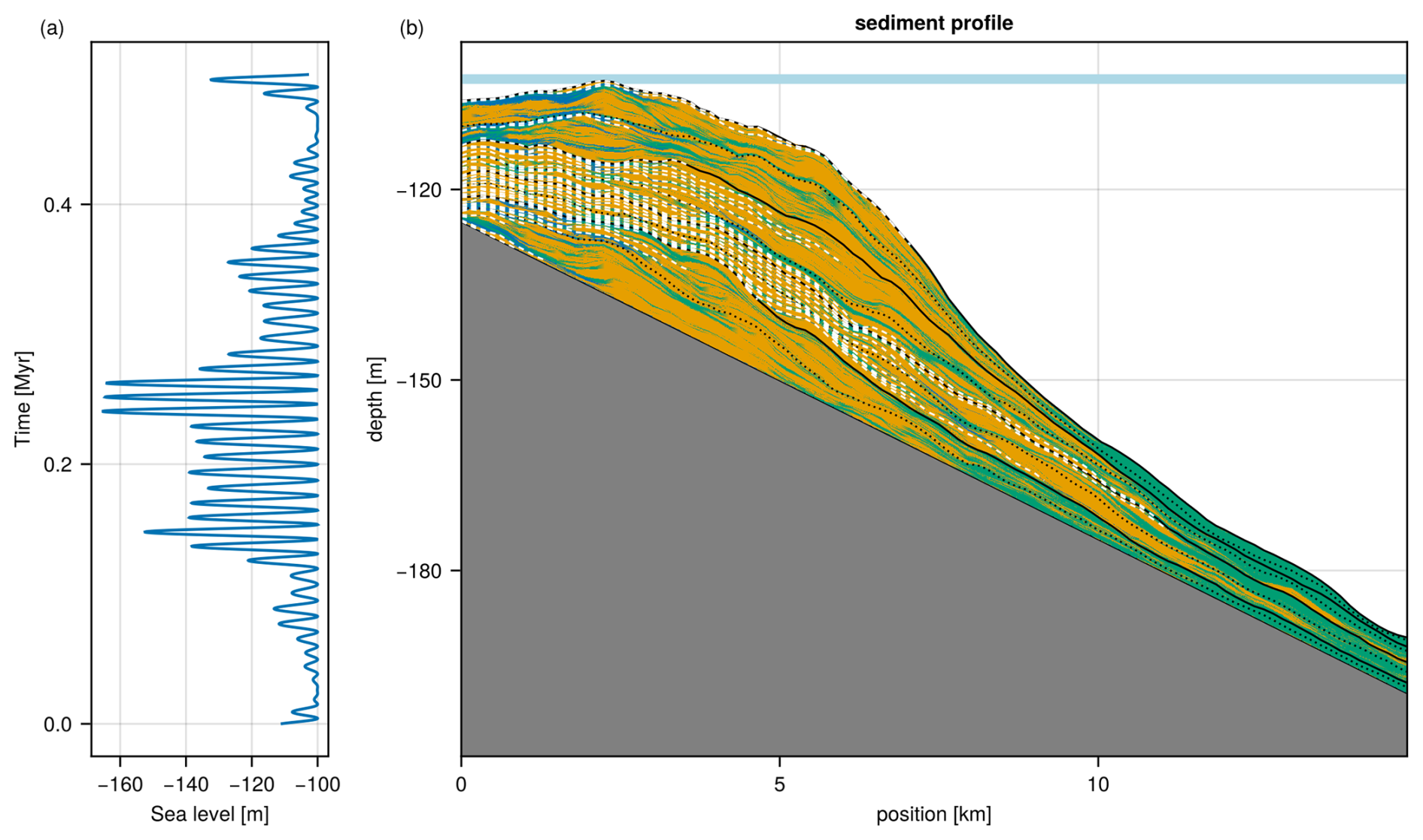
Figure 13 Platform generated using the daily mean insolation during June solstice at the 25° N latitude for a period of 1 Myr starting in 1950 and using a sea level curve obtained by amplifying the insolation values. Panel (a) shows the insolation-based amplified sea level curve. Panel (b) shows the corresponding output stratigraphy.

As default, we use insolation of 400 W m⁻², which is approximately equivalent to the 2000 µE m⁻² s⁻¹ used by Bosscher and Schlager (1992). This is representative of insolation on the sea surface at midday in the tropics. However, insolation varies with the position of the Earth with respect to the Sun and over geological timescales this variation may affect the patterns of sediment production. Incoming solar radiation can be used as an input vector to modulate production. CarboKitten is agnostic with respect to the source of this information. As an example in Fig. 13, here we use the daily mean insolation on June solstice, calculated using the astronomical solution by Laskar (2004), obtained through the R package palinsol (Crucifix, 2023). Here we obtain it for the coming million year (starting in 1950, which is when the astronomical solution starts) at the 25° N latitude and use the total solar irradiance value of 1361 kW m⁻². Variation in solar irradiance is so small that it would hardly manifest itself if linearly propagated to the sea level curve. A universal transfer function describing the relationship between insolation and sea level does not exist. For the purpose of illustrating the functionality of the model, we calculate the sea level as an amplified insolation value. The amplification is chosen arbitrarily as the square of the insolation anomaly, with the anomaly being the deviation from mean irradiation.

The insolation file can be read into a CarboKitten script defining the model to be run. The alternative is calling R directly from Julia using RCall.jl.

6.3 Wave induced transport

We model the transport by waves by setting the velocity v_f and shear s_f components in Eq. (7). In this analysis we forego claims on any level of realism with respect to the true long term effects of wave transport, rather we study the behaviour of the model under an imposed additional velocity component. Our use of the term wave transport should also be understood as such.

Considering the long timescales we are working with, we limit ourselves to a highly simplified model, with the goal of achieving an effect comparable with that of wave-induced transport. Given the timescales for which the model is developed, with time steps of the order of 100 years, a more physical representation of wave-induced transport is not possible. By necessity, the result imitates the time-averaged effect of transport.

Our approach is illustrated with an example of an atoll, starting with a conical topography and periodic boundaries.

Here we try three different velocity profiles: first no onshore component, second a constant vector that does not depend on water depth, and third an attempt at a more realistic scenario.

The following equation is the well known phase velocity of waves as a function of depth from linear wave theory,

$$\begin{array}{}\text{(13)}& v\left(w\right)=\sqrt{{\displaystyle \frac{\mathit{\lambda }g}{k}}}\tanh \left(kw\right),\end{array}$$

where w is the water depth, k the wave number ($k=\mathrm{2}\mathit{\pi }/\mathit{\lambda }$), and g is the gravitational acceleration. This velocity is the phase-velocity of surface waves, given the total depth of the water. To evaluate the transport velocity at deeper levels, we multiply the phase velocity with a factor exp (−kw) to account for Stokes drift:

$$\begin{array}{}\text{(14)}& v_{\mathrm{f}}=A_{\mathrm{f}}\exp (-kw)\tanh \left(kw\right),\end{array}$$

where A_f is the facies-dependent maximum transport velocity. The k parameter can be tweaked to set the depth at which the maximum transport velocity is attained. We assume most of the sediment transport happens close to the sea floor. This profile is chosen for its assymptotic properties: at high water depth the transport velocity converges to zero, while the decrease in wave velocity towards shallow depths ensures that there is a net influx of material close to the shore. An example of this profile is shown in Fig. 14.

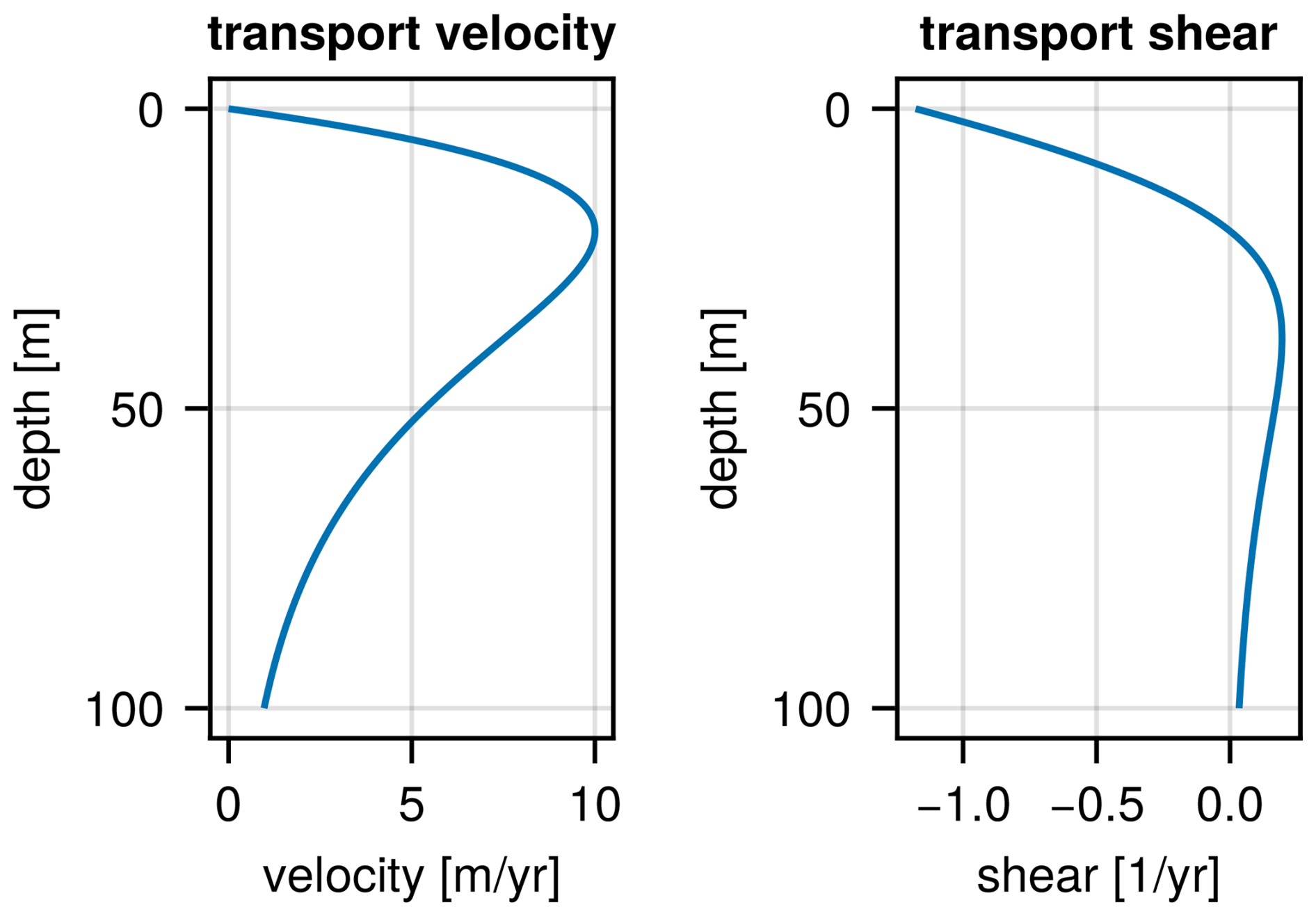
Figure 14 Depth profile of wave velocity and shear. The velocity profile was taylored to have a maximum of 10 m yr⁻¹ at a depth of 20 m. Where the shear is negative (assuming transport is directed onshore), there is a net accumulation of sediment.

We model the formation of an atoll for three cases: no wave transport, constant transport directed west-ward (along the x-axis), and a depth dependent velocity profile. The results of this experiment are shown in Fig. 15. Velocity functions are configured for each facies separately. We found that it was quite easy to create an unstable model by choosing on-shore velocities too high, particularly in the case where the velocity shear is non-zero. Build-up of material due to high on-shore velocity can be compensated by setting a higher facies transport coefficient.

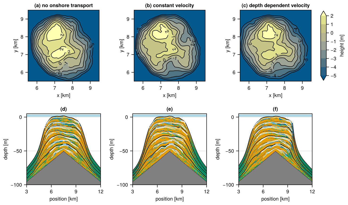
Figure 15 Topography and sediment profiles of an atoll. We ran the same model three times with different on-shore velocity profiles: no on-shore transport, a constant velocity and lastly the profile given in Eq. (14). The top row (a–c) show the topography of the generated island, while the bottom row (d–f) show the corresponding sediment profiles. Small differences in water depth may get amplified exponentially by the production model, so we see some stark differences in the outcomes for the different velocity profiles. Comparing the first (without additional transport vector) and second case (flat profile), we see little change in the overall shape of the atoll, but there is a clear difference in the facies composition at the transition between oligophotic (yellow) and aphotic (green) dominated areas. In the third case we see the topography changed significantly between the leeward and windward sides of the atoll, where the slope is much steeper. Also the facies composition changed further: most notably we see a relative prominence of euphotic (blue) facies on the windward side of the island.

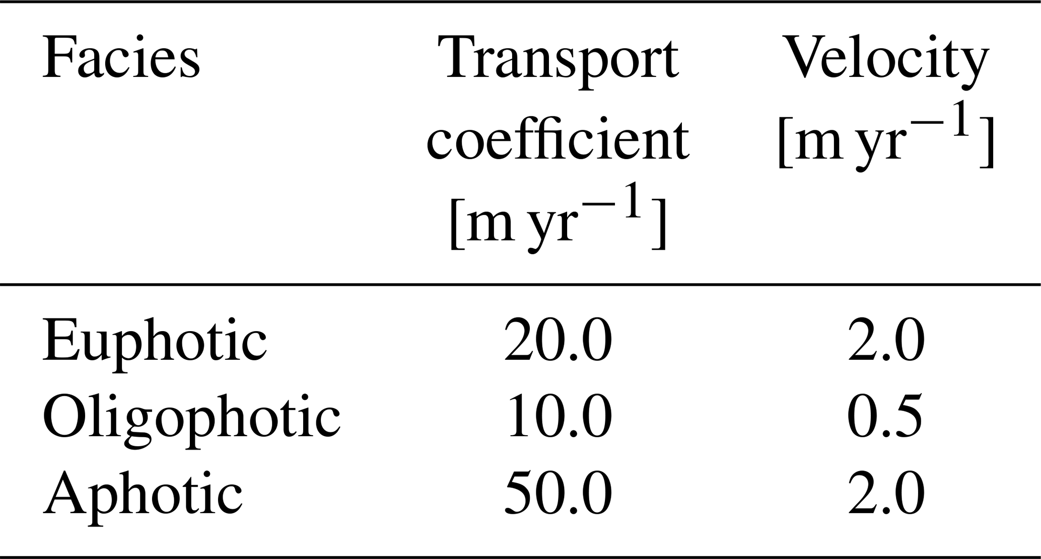
If we assume that both the facies transport coefficient and the wave velocity are some constant times a hypothetical carrying water velocity, it would be fitting to make sure that for each facies the transport coefficient and velocity have a similar proportion. In our experiment we took the values listed in Table 4. It is very hard to find proper motivation for any of these values, but by changing them we can learn more about the mechanisms and systematic behaviours of the model and by extension possibly learn more about the formation of carbonate platforms and study sensitivities in their observed stratigraphic patterns.

Table 4 Chosen parameters to generate results in Fig. 15. We used a lithification time of 100 year and a disintegration rate of 50 m Myr⁻¹.

7 Conclusions

CarboKitten is a new Open Source stratigraphic forward model dedicated for carbonate depositional environments and modeling of timescales between centuries and millions of years. It integrates previous, well-tested approaches used by the community, i.e. the production model by Bosscher and Schlager (1992) and the generation of spatial heterogeneity proposed by Burgess (2013) with a new approach to sediment transport, based on the concept of the active layer by Paola et al. (1992). The software allows modeling and visualization accessible to laptop users, including attractive plotting functions for common use-cases in stratigraphy and sedimentology, such as Wheeler diagrams, age-depth models and stratigraphic columns. CarboKitten uses heuristics to approximate the dynamics of carbonate production, wave transport and biologically driven spatial heterogeneity. The algorithms do not replicate the physical and biological processes behind these phenomena, but allow obtaining results imitating them at timescales at which they cannot be observed directly.

CarboKitten fills a gap identified at the outset of this manuscript: an Open Source, modular, performant stratiraphic forward model dedicated to carbonate platforms and their idiosyncracies. It complements the landscape of Earth-surface models such as Landlab (Hobley et al., 2017; Barnhart et al., 2020) and the broader suite of tools developed and maintained by the Community Surface Dynamics Modeling System (CSDMS). Future opportunities for CarboKitten include integration with Landlab and other CSDMS components.

At this stage, CarboKitten's primary value lies not in a realistic replication of empirical stratigraphic architectures, but in its utility for testing hypotheses on the formation of the carbonate geological record and on our own understanding on its governing processes. Further work is needed to allow more detailed reconstructions of known geological situations. Among future refinements are empirical validation of transport and production values or storing the history of sediment transport to track autochthonous and allochthonous sediment.

CarboKitten offers a powerful tool to ground-truth concepts of how time is represented in the physical rock record (e.g., Burgess, 2008; Burgess et al., 2019; Sultana et al., 2022) and constrain the limits of reconstruction of processes such as evolution (Holland and Patzkowsky, 1999; Hannisdal, 2006; Hohmann et al., 2024), climate change, or other aspects of the changing Earth's environment (e.g., Kemp et al., 2016; Kemp and Van Manen, 2019; Myrow and Grotzinger, 2000; Geyman et al., 2021; Husinec et al., 2023; Curtis et al., 2025). We hope the accessibility and reproducibility of CarboKitten simulations will encourage wider use of stratigraphic forward models towards a hypothetico-deductive research in stratigraphy.

Appendix A: Derivation of transport equations

Our basic assumption is that the sediment flux scales linearly with the local bathymetric gradient and the concentration of sediment in the active layer,

$$\begin{array}{}\text{(A1)}& {\mathit{q}}_{\mathrm{f}}\left(x\right)=-d_{\mathrm{f}}{C}_{\mathrm{f}}\left(x\right)\mathbf{\nabla }\mathit{\eta }\left(x\right)+{\mathit{v}}_{\mathrm{f}}\left(w\right(x\left)\right))C_{\mathrm{f}},\end{array}$$

where C_f is the active sediment amount per facies (all “f” suffixes indicate facies dependent quantities), d_f the transport (diffusivity) coefficient, η(x) the bathymetry, and v_f the wave velocity as a function of water depth w(x). Since the water depth and bathymetry differ at any time by a constant an a minus sign, $\mathbf{\nabla }w=-\mathbf{\nabla }\mathit{\eta }$, it is advantageous to write the equation completely in terms of w,

$$\begin{array}{}\text{(A2)}& {\mathit{q}}_{\mathrm{f}}\left(x\right)=C_{\mathrm{f}}\left(x\right)\left(d_{\mathrm{f}}\mathbf{\nabla }w\left(x\right)+{\mathit{v}}_{\mathrm{f}}\left(w\right(x\left)\right)\right).\end{array}$$

We can transform this assumption in to an advection equation by considering the continuity equation,

$$\begin{array}{}\text{(A3)}& {\displaystyle \frac{\partial C_{\mathrm{f}}\left(x\right)}{\partial t}}=-\mathbf{\nabla }\cdot {\mathit{q}}_{\mathrm{f}}\left(x\right)+P\left(x\right),\end{array}$$

where P(x) is the sediment production rate (including disintegration). We can leave the production out of consideration for the moment. Also, for readability, we will be dropping the function dependencies on x and in our notation, as well as the “f” suffix, considering each facies independently. Using the product rule,

$$\begin{array}{}\text{(A4)}& {\displaystyle \frac{\partial C}{\partial t}}=-\mathbf{\nabla }C\cdot (d\mathbf{\nabla }w+\mathit{v}(w\left)\right)-C\left(d{\mathrm{\nabla }}^{\mathrm{2}}w+\mathbf{\nabla }\cdot \mathit{v}\left(w\right)\right).\end{array}$$

Now, we demand that the user provide the derivative $\mathit{s}\left(w\right)={\mathit{v}}^{\prime }\left(w\right)$, so applying the chain rule we can write,

$$\begin{array}{}\text{(A5)}& \mathbf{\nabla }\cdot \mathit{v}\left(w\right)=\mathbf{\nabla }w\cdot \mathit{s}\left(w\right).\end{array}$$

Substituting that into the previous equation and collecting terms by C and ∇C brings us to Eq. (7),

$$\begin{array}{}\text{(A6)}& {\displaystyle \frac{\partial C}{\partial t}}=-(d\mathbf{\nabla }w+\mathit{v}(w\left)\right)\cdot \mathbf{\nabla }C-\left(d{\mathrm{\nabla }}^{\mathrm{2}}w+\mathbf{\nabla }w\cdot \mathit{s}\left(w\right)\right)C.\end{array}$$

Appendix B: Model parameters

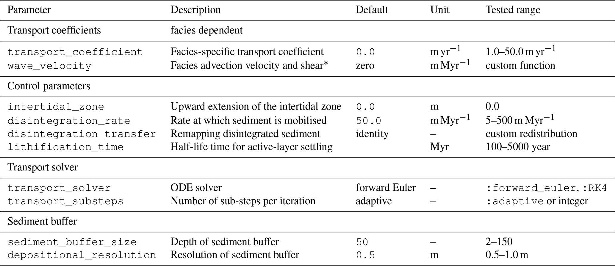
For completeness we give an overview of the paramaters that enter CarboKitten's main model called ALCAP (Active Layer, Cellular Automaton and Production), at the time of writing the most extensive model in CarboKitten. We split these parameters in three categories. The global parameters deal with the grid geometry, time integration and external forcings (see Table B1). A second set of parameters are specified for each facies individually, e.g. production rates and CA behaviour (see Table B2). The third category concerns everything related to the transport model (see Table B3). Note that the transport coefficients are facies dependent, all others are global parameters.

Table B1 Grid and time parameters. Parameters marked with ^*  can be specified as a constant, table or Julia function. Parameters that have – as default value are required.

Table B2 Facies parameters.

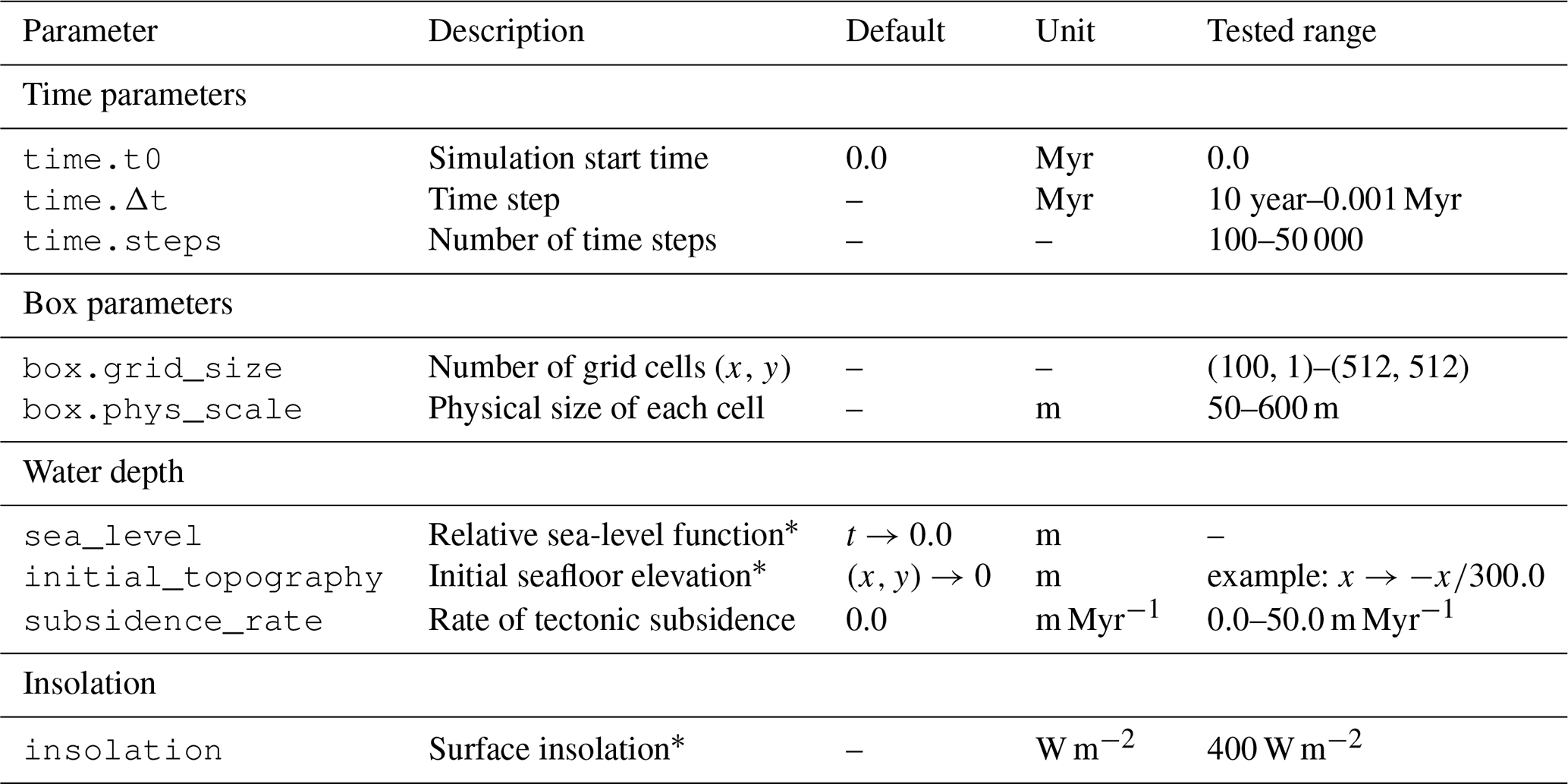
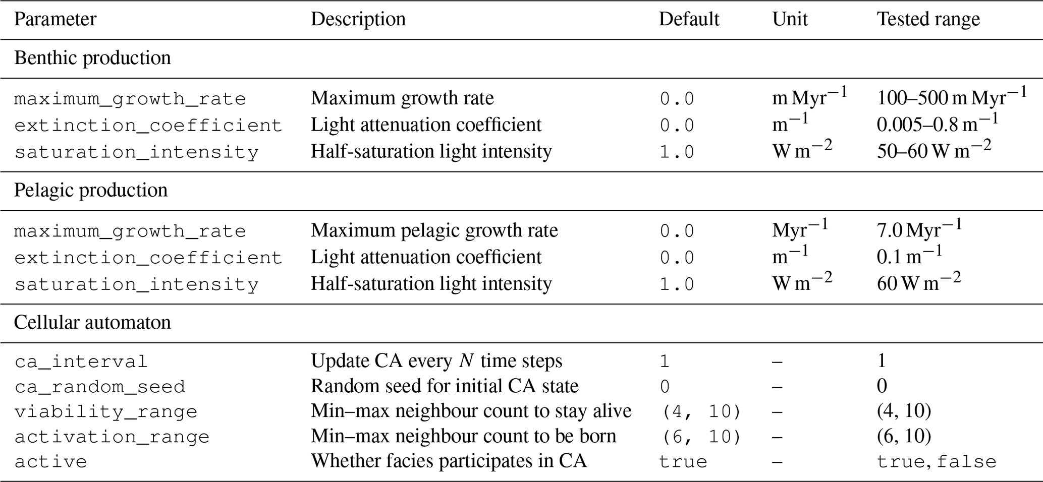
Table B3 Transport parameters. ^* The user needs to specify both velocity and its derivative as function of water depth.