New framework for benchmarking decadal predictions leveraging the PCMDI Metric Package with interactive visualization

Reliable climate predictions across multiple timescales are increasingly critical as climate-related risks continue to rise. With the growing number and diversity of climate prediction systems, systematic intercomparison has become essential. Here, we present a comprehensive evaluation framework based on the PCMDI Metric Package to assess the performance of multiple decadal climate prediction systems. Unlike uninitialized simulations, initialized predictions exhibit bias and predictive skill that evolve with forecast lead time. To address this, we introduce (1) model-by-lead-time portrait plots, which efficiently summarize metrics of global temperature, precipitation, and Arctic/Antarctic sea-ice extent, and (2) an HTML-based interactive visualization platform that provides detailed regional and seasonal diagnostics of model bias, skill scores, and ensemble spread for each model and lead time. Comparisons with uninitialized simulations further quantify the relative impacts of initialization and external forcing on prediction skill. The proposed framework provides a scalable and transparent approach for multi-model climate prediction assessments and can be readily extended to a wide range of operational and research forecasting systems.

1 Introduction

As society faces growing challenges related to extreme climate conditions, the demand for accurate climate predictions is increasing. To support climate-informed decision-making, operational forecast centers and research institutions around the world now routinely provide subseasonal-to-seasonal climate predictions (e.g., Buontempo et al., 2022; Xue et al., 2025; Yhang et al., 2025) and long-term climate projections (e.g., IPCC, 2013) to inform climate adaptation and mitigation strategies. Decadal climate prediction, also known as near-term climate prediction, typically covers the period from one to ten years ahead. It bridges the gap between the seasonal predictions and long-term projections (Meehl et al., 2021). As such, decadal climate prediction plays a critical role in enabling seamless climate services and guiding climate risk management (Dunstone et al., 2022; Solaraju-Murali et al., 2022; O'Kane et al., 2023).

In recognition of this need, major climate modeling centers began offering decadal climate prediction experiments in the early 2010s (Smith et al., 2013). Starting in 2021, the World Meteorological Organization (WMO) has provided annual climate outlooks extending up to five years ahead (Hermanson et al., 2022). Furthermore, the Decadal Climate Prediction Project (DCPP; Boer et al., 2016), which participated in the Coupled Model Intercomparison Project Phase 6 (CMIP6), is one of the coordinated international efforts that support the systematic production and comparison of initialized decadal prediction experiments. As decadal climate prediction is expected to remain a key component of the upcoming CMIP Phase 7 (Dunne et al., 2025), the number of participating prediction systems continues to increase.

Reliable decadal climate predictions require accurate information from both initial conditions and external forcing (Keenlyside et al., 2008; Corti et al., 2015; Klavans et al., 2021; Meehl et al., 2021). Initialization is particularly important for representing slow components of the climate system, such as the ocean, sea ice, and land surface, which can store anomalies and influence climate variability years in advance. These initialized climate predictions behave fundamentally differently from uninitialized climate projections. Since the observation-constrained initial state gradually drifts toward the model's climatology, initialized predictions exhibit time-evolving biases, systematic drift, and variations in prediction skill across lead times (Kharin et al., 2012; Sanchez-Gomez et al., 2016; Nadiga et al., 2019; Meehl et al., 2022). These lead-time-dependent characteristics add complexity to model evaluation and require specialized metrics capable of separating drift effects, externally forced signals, and actual predictive skill.

Over the past decades, the climate research community has developed a wide range of diagnostic frameworks and standardized metrics to evaluate long-term climate simulations, particularly for the CMIP historical experiments. These efforts include benchmarking-oriented diagnostics that quantify systematic model performance using standardized metrics and intercomparison frameworks (e.g., Gleckler et al., 2008; Eyring et al., 2020) and process-based diagnostics that investigate the physical mechanisms underlying model biases and variability (e.g., Maloney et al., 2019; Planton et al., 2021). Several community tools have been developed as reusable software packages, including the Program for Climate Model Diagnosis and Intercomparison (PCMDI) Metrics Package (PMP; Lee et al., 2024), the Earth System Model Evaluation Tool (ESMValTool; Eyring et al., 2020), and related CMIP diagnostics frameworks (Maher et al., 2025; Hassler et al., 2026).

Benchmarking diagnostics provide a standardized and reproducible framework for comparing model performance. However, most existing evaluation frameworks primarily target uninitialized historical simulations and long-term climate projections. These frameworks' current capabilities do not fully address the unique characteristics of initialized decadal predictions, where the forecast drifts, the time-evolving biases, and the lead-time-dependent prediction skill require their own customized and specialized evaluation strategies. To address this gap, we propose a new evaluation framework that could assess multi-model initialized decadal prediction systems systematically and comprehensively, leveraging the established community tool for the CMIP evaluation, using some of the PMP's approach and capabilities.

2 Data and Methodology

We describe retrospective decadal predictions and observation datasets in Sect. 2.1. The measures of model bias, prediction skill, and spread are also presented in Sect. 2.2 and 2.3.

2.1 Model and observation datasets

This study uses 11 models that participate in the DCPP. Each model includes at least three ensemble members and up to ten ensemble members, depending on the variables and simulations (see Table 1). We analyze retrospective predictions (hindcasts) initialized each November from 1960 to 2016. Two models (CanESM5 and IPSL-CM6A-LR) were initialized in January of the following year. Following the CMIP6 convention, each initialization is denoted as sYEAR; for instance, s1960 refers to the initialization in November 1960 or January 1961. These hindcasts use external boundary forcings from the CMIP6 historical experiment. Beyond the historical period (after 2015), the SSP2-4.5 scenario forcing is applied. Furthermore, we use historical simulations to evaluate the impact of external radiative forcing on predictive skills by comparing them with the initialized predictions.

Table 1 Brief description of the models and three variables (TAS: surface air temperature, PR: precipitation, SIC: sea ice concentration) used in this study. Ten ensemble members are used, and variables with fewer than ten members are indicated in parentheses.

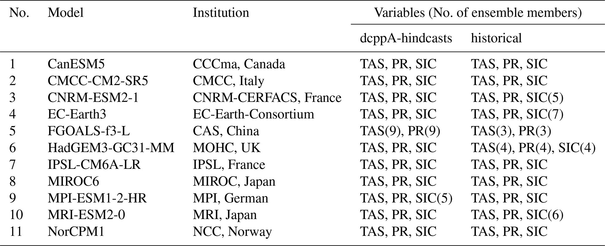
The fifth-generation European Centre for Medium-Range Weather Forecasts atmospheric reanalysis (ERA5; Hersbach et al., 2020) is used as reference data for surface air temperature (TAS) from 1961 to 2021. Precipitation (PR) data are obtained from the Global Precipitation Climatology Project (GPCP; Huffman et al., 2023) for the period from 1979 to 2021. Sea ice concentration (SIC) is taken from the Hadley Centre Sea Ice and Sea Surface Temperature dataset (HadISST_ICE; Rayner et al., 2003) for the period of 1961–2021. All modeled and observed variables, except for SIC, are interpolated to a uniform 2.5° × 2.5° grid before the analysis.

2.2 Measure of model bias

Model biases are evaluated for long-term climatology and trends. Bias in long-term climatology (hereafter, mean bias) is calculated for TAS and PR at each grid cell. It is defined as the difference between the model and observed climatology for each lead year during the common period of 1981–2010. For example, the mean bias for lead year 1 (LY1) is calculated using the simulations from s1980 to s2009, while that for lead year 10 (LY10) is calculated using the simulations from s1971 to s2000. Lead times up to ten years are analyzed, except for two models (CNRM-ESM2-1 and MRI-ESM2-0), which are evaluated up to five years.

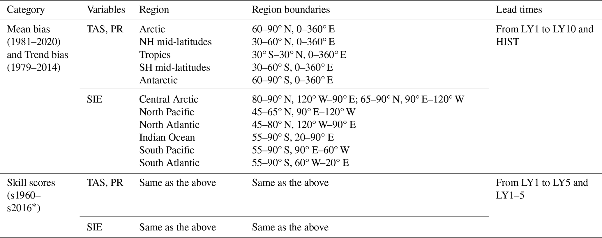
To examine regional and seasonal variations, gridded monthly data are used to calculate the mean bias and then averaged over space and time. After annual averaging, the mean biases are averaged within five latitudinal zones and visualized as a function of lead years. These zones are defined as the Arctic (60–90° N), the Northern Hemisphere (NH) mid-latitudes (30–60° N), the tropics (30° S–30° N), the Southern Hemisphere (SH) mid-latitudes (30–60° S), and the Antarctic (60–90° S) (see also Table 2). Interactive plots show the global maps of mean biases, which are produced by averaging data over two-month periods to illustrate their regional and seasonal variations.

Table 2 Summary of the temporal and spatial definitions for the variables evaluated in this study. Sea-ice extent (SIE) followed the definition by Ivanova et al. (2016). Mean and trend biases are analyzed for Lead Year (LY) 1 to 10 and historical simulations (HIST). Skill scores are analyzed for LY1 to LY5 and the 5-year averages (LY1–5). The numbers and terms in parentheses in the first column refer to the periods and experimental names used for evaluating bias and skill scores, respectively.

^* s1960–s2016 for TAS and SIE, s1978–s2016 for PR.

Bias in long-term trend (hereafter, trend bias) is defined as the difference in the least squares fitting coefficients between the model and observation. Trend biases in monthly TAS and PR are calculated at each grid cell for the common period of 1979–2014, and then averaged over space and time. Similar to the mean bias, the trend biases are averaged within the five latitudinal zones and visualized as a function of lead years. Interactive plots are also used to examine regional and seasonal variations in the trend bias.

Unlike TAS and PR, the monthly SIC is averaged first over predefined regions. This regional averaging approach further enables consistent comparison across heterogeneous native ocean grids without requiring an additional remapping procedure. According to Ivanova et al. (2016), both the Arctic and the Antarctic are divided into three regions to examine the mean and trend biases (see also Table 2). In each domain, the sea ice extent (SIE) is defined as the region in which SIC exceeds 15 %. Interactive plots display the SIC climatology and trend distribution. These maps are represented on the raw grid of model data as shading, together with the observed values shown as contours. The results are presented in bimonthly periods to highlight seasonal variations.

2.3 Measure of prediction skill and spread

Initialized decadal predictions are known to exhibit systematic forecast drift as the simulations diverge from the observation-constrained initial state and approach the model's preferred climatology. Following the standard procedure used in decadal prediction studies (Goddard et al., 2013; Choi and Son, 2022), the mean climatological bias for the period 1981–2010 is removed for each lead month before calculating the metrics.

In contrast, long-term trend biases are intentionally retained in the current framework. Unlike the mean climatological drift, the trend biases may evolve nonlinearly in lead time, reflecting the complex interactions between the externally forced signals, internally generated variability, and model adjustment processes. Rather than correcting these effects explicitly, this study compares evaluation metrics between initialized decadal hindcasts and uninitialized historical simulations.

To allow for as many initializations as possible for skill evaluation, we use the initialized hindcasts of s1960–s2016 (s1978–s2016 for precipitation). For LY1, the corresponding observations cover the period from 1961 to 2017. For lead year 5 (LY5), the corresponding observations span from 1965 to 2021. To verify the predictive performance of long-term changes, the skill scores are further calculated for an average of lead years one through five (LY1–5).

Deterministic prediction skill is evaluated quantitatively using two metrics: the anomaly correlation coefficient (ACC) and the mean squared skill score (MSSS). These metrics are defined as follows:

$$\begin{array}{}\text{(1)}& {\displaystyle }\begin{array}{rl}& {\mathrm{ACC}}_{\mathit{\tau }}\left(M,O\right)=\\ & {\displaystyle \frac{\frac{\mathrm{1}}{n}{\sum }_{j=\mathrm{1}}^n(M_{j\mathit{\tau }}-{\stackrel{\mathrm{‾}}{M}}_{\mathit{\tau }})(O_{j\mathit{\tau }}-{\stackrel{\mathrm{‾}}{O}}_{\mathit{\tau }})}{\sqrt{\frac{\mathrm{1}}{n}{\sum }_{j=\mathrm{1}}^n(M_{j\mathit{\tau }}-{\stackrel{\mathrm{‾}}{M}}_{\mathit{\tau }}{)}^{\mathrm{2}}}\sqrt{\frac{\mathrm{1}}{n}{\sum }_{j=\mathrm{1}}^n(O_{j\mathit{\tau }}-{\stackrel{\mathrm{‾}}{O}}_{\mathit{\tau }}{)}^{\mathrm{2}}}}},\end{array}\text{(2)}& {\displaystyle }\begin{array}{rl}& {\mathrm{MSSS}}_{\mathit{\tau }}\left(M,O\right)=\mathrm{1}-{\displaystyle \frac{{\mathrm{MSE}}_{\mathit{\tau }}\left(M\right)}{{\mathrm{MSE}}_{\mathit{\tau }}\left(\stackrel{\mathrm{‾}}{O}\right)}}\\ & =\mathrm{1}-{\displaystyle \frac{\frac{\mathrm{1}}{n}{\sum }_{j=\mathrm{1}}^n{\left[\left(M_{j\mathit{\tau }}-{\stackrel{\mathrm{‾}}{M}}_{\mathit{\tau }}\right)-\left(O_{j\mathit{\tau }}-{\stackrel{\mathrm{‾}}{O}}_{\mathit{\tau }}\right)\right]}^{\mathrm{2}}}{\frac{\mathrm{1}}{n}{\sum }_{j=\mathrm{1}}^n(O_{j\mathit{\tau }}-{\stackrel{\mathrm{‾}}{O}}_{\mathit{\tau }}{)}^{\mathrm{2}}}}\end{array}\end{array}$$

where M and O are the ensemble-mean predictions and observations, respectively. Since the annual average is performed for both M and O, the skill scores are not dependent on the seasons. The subscript τ is the forecast lead time. The subscript j represents the initialization year, and n represents the total number of initializations. Therefore, n is set to 57 for TAS and SIE (39 for PR). The overbar indicates the long-term average over the entire period. The MSSS is a function of the mean squared error (MSE); mathematically, it combines the ACC and the conditional bias (Goddard et al., 2013). Therefore, while the ACC quantifies the model's predictive ability in terms of the phase of variability, the MSSS further estimates both the phase and amplitude of variability (Choi et al., 2016). Both the ACC and MSSS are 1 for perfect predictions. The prediction skill of SIE is further evaluated using root mean square error (RMSE), defined as the square root of the numerator in the second term of Eq. (2).

In addition, the ratio of predictable components (RPC) between the real and model worlds is computed to measure the signal-to-noise paradox of climate predictions (Weisheimer et al., 2024). It is defined by comparing the predictable component of the observations (PC_Obs) with the predictable component of the model (PC_Model) as follows:

$$\begin{array}{}\text{(3)}& \mathrm{RPC}={\displaystyle \frac{{\mathrm{PC}}_{\mathrm{Obs}}}{{\mathrm{PC}}_{\mathrm{Model}}}}\ge {\displaystyle \frac{\mathrm{ACC}(M,O)}{\sqrt{{\mathit{\sigma }}_{\mathrm{signal}}^{\mathrm{2}}/{\mathit{\sigma }}_{\mathrm{total}}^{\mathrm{2}}}}}\approx {\displaystyle \frac{\mathrm{ACC}(M,O)}{\mathrm{ACC}(M,M^{\prime })}}.\end{array}$$

The lower bound of PC_Obs can be estimated by the ACC between ensemble-mean predictions (M) and observations (O), as the ACC² (M, O) reflects the proportion of the observed variance explained by ensemble-mean predictions (Eade et al., 2014). Similarly, PC_Model can be identical to the expected average of ACCs between ensemble-mean predictions (M) and individual predictions (M^′). If the RPC is significantly greater than one, then the observations are more predictable than the model ensemble predictions, constituting the signal-to-noise paradox (Weisheimer et al., 2024).

2.4 Interactive visualization

Unlike uninitialized simulations (e.g., historical experiments), initialized decadal predictions exhibit evolution in model biases and prediction skill that depends on lead time. Consequently, evaluation outputs are substantially larger and more multidimensional, considering lead times, models, and metrics simultaneously. Therefore, static figures alone are not very efficient for exploring and interpreting the full evaluation results.

To address this challenge, we have developed an HTML-based interactive visualization framework following the PMP approach. We used the Python library Bokeh (https://bokeh.org/, last access: 6 July 2026) to enable flexible exploration of the benchmarking diagnostics. The interface allows users to dynamically compare models, lead times, and diagnostic metrics through interactive selection and navigation tools. With this design, researchers can rapidly detect systematic model behaviors, lead-time drift, and differences between models – insights that are hard to capture with conventional static plots.

The framework supports reproducible and scalable evaluation workflows for large multi-model prediction archives such as CMIP6 DCPP. By leveraging browser-based interactive graphics, the visualization outputs can be easily shared, archived, and extended to future prediction systems and additional diagnostic metrics. All interactive figures are available at https://pcmdi.llnl.gov/metrics/dcpp (last access: 20 June 2026).

3 Results

3.1 Mean bias

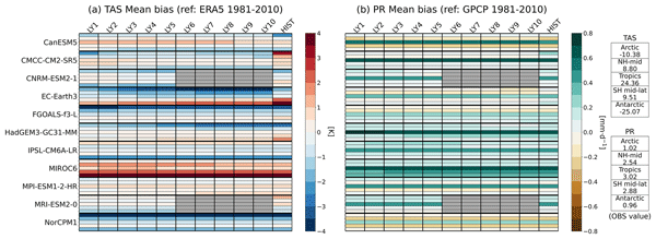
Figure 1a presents a model-by-lead-time portrait plot of the mean bias in TAS. The rightmost column corresponds to the mean bias derived from the historical experiments (HIST), enabling a comparison between the time-dependent mean bias of initialized decadal hindcasts and the systematic climatological bias of HIST. The five inner boxes within each cell, from top to bottom, correspond to the Arctic, NH mid-latitudes, tropics, SH mid-latitudes, and Antarctic regions. This allows for an inspection of the latitude-dependent bias structure. In general, biases tend to be larger in the polar regions than in the low-to-mid latitudes.

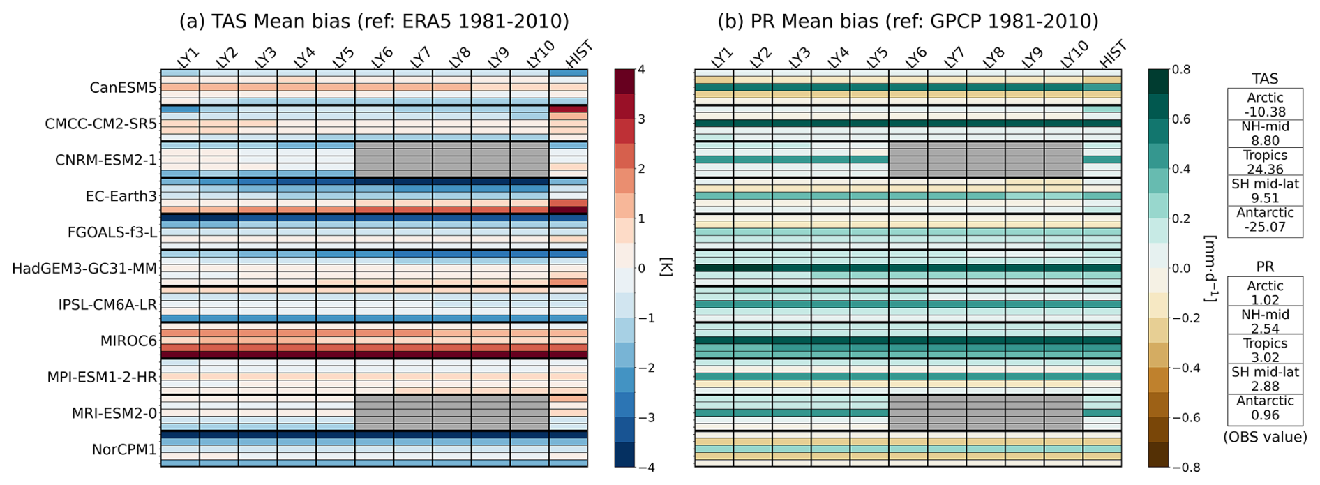
Figure 1 (a) Model-by-lead-time portrait plot showing the mean bias of TAS over the period 1981–2010. The mean bias is calculated as a function of LY over the globe and five subregions: Arctic (60–90° N), the Northern Hemisphere mid-latitudes (30–60° N), the Tropics (30° S–30° N), the Southern Hemisphere mid-latitudes (30–60° S), and Antarctic (60–90° S). The rightmost column indicates the mean bias from HIST for the same period. ERA5 is used as the reference dataset. Units are [K]. (b) Same as (a), but for the precipitation (PR). GPCP is used as the reference dataset. Units are [mm d⁻¹]. Mean bias is calculated for each month and each grid cell, and then annual and area averages are taken. Note that labels are top-aligned to optimize visibility within the scrolling web interface. Gray shading between LY6 and LY10 for CNRM-ESM2-1 and MRI-ESM2-0 indicates missing data because only 5-year predictions are available. Numbers in boxes on the right side of the figure represent the observed values. All individual subplots relevant to portrait plots can be interactively visualized on the https://pcmdi.llnl.gov/metrics/dcpp (last access: 20 June 2026).

Although some models exhibit clear lead-time-dependent bias growth (e.g., polar regions in EC-Earth3 and HadGEM3-GC31-MM), the evolution of mean bias is not always visually pronounced in Fig. 1. This partly reflects the substantial inter-model spread represented using a common color scale, but also the rapid adjustment of initialized forecasts toward the model climatology, particularly in the ocean component, where mean biases can develop within the first several months of integration (Ma et al., 2021).

As lead time increases, initialized predictions generally tend to drift from the observed initial state toward the model's preferred coupled equilibrium state. However, the evolution of mean bias is not necessarily monotonic, as it can be affected by initialization shocks and adjustment processes during the forecast period (e.g., Mulholland et al., 2015). Additionally, coupled ocean–atmosphere feedbacks and internally generated ocean variability may partially compensate for inherited model biases. Consequently, some models exhibit even decreasing mean biases with lead time, especially for tropical TAS (e.g., CanESM5, CMCC-CM2-SR5, FGOALS-f3-L in Fig. 1a), rather than the monotonic growth expected from climatological drift alone.

Figure 1b shows the mean bias in PR. Given the fact that simulated precipitation is affected by model physics and dynamics, as well as complicated nonlinear surface processes (Li et al., 2020; Tian and Dong, 2020), the magnitude of the precipitation bias does not necessarily correspond to the magnitude of the temperature bias. Instead, Fig. 1b showcases more of the known pattern of systematic precipitation biases in climate models than the substantial lead-time-dependent variations. Most models exhibit wet biases in the tropics and dry biases in the mid-latitudes. Tropical wet biases are commonly associated with the excessive double Intertropical Convergence Zone (ITCZ), which has been linked to multiple factors, including deficiencies in dynamical circulation and thermodynamic processes (Zhang et al., 2015; Samanta et al., 2019). In contrast, dry biases in the mid-latitudes are often related to land–atmosphere feedbacks associated with summer warm biases (Mueller and Seneviratne, 2014; Lin et al., 2017), as well as atmospheric circulation biases associated with storm-track position and intensity (Priestley et al., 2020; Schemm, 2023).

Figure 2 displays the mean bias of SIE in the Arctic and Antarctic regions. While the observed SIE exhibits a similar magnitude between the two regions (Arctic: ∼ 11.98 × 10⁶ km²; Antarctic: ∼ 12.59 × 10⁶ km²; the Arctic SIE is approximately 95 % of the Antarctic SIE), the mean bias and inter-model spread tend to be larger in the Antarctic. In some models, the SIE mean bias is closely related to the TAS mean bias in the polar regions. For example, EC-Earth3 shows an expansion of Arctic sea ice, especially in the North Atlantic. This is likely associated with the growth of the Arctic cold bias at longer lead times (see also Fig. 1a). Conversely, the Antarctic warm bias in MIROC6 is pronounced and corresponds to widespread sea ice retreat. HadGEM3-GC31-MM and EC-Earth3 exhibit a greater reduction in Antarctic sea ice in HIST than in the initialized decadal hindcasts. This is consistent with the stronger Antarctic warm bias in the HIST simulation (see also Fig. 1a).

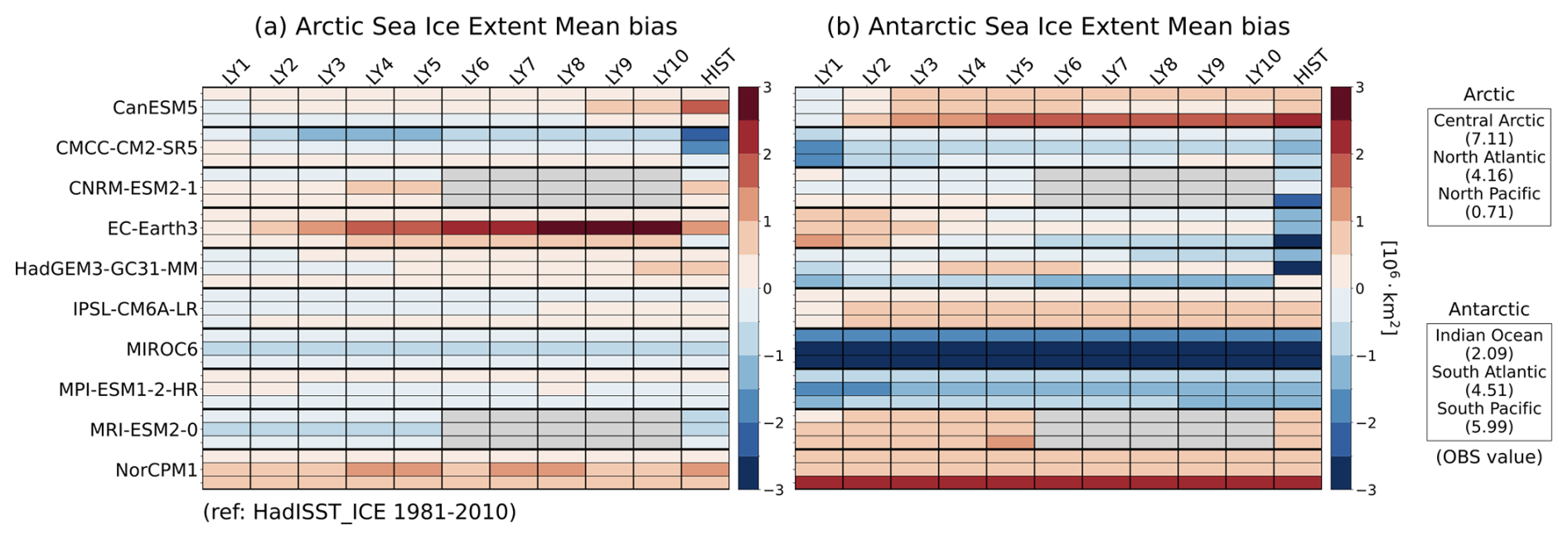
Figure 2 Model-by-lead-time portrait plot showing the mean bias in sea-ice extent over the period 1981–2010. Area averages are firstly taken for three predetermined subregions: (a) the Arctic and (b) the Antarctic, for each month. Then, the annual averages are taken at each LY. The rightmost column indicates the mean bias from HIST for the same period. HadISST_ICE is used as the reference dataset. Units are [10⁶ km²]. Numbers in parentheses on the right side of the figure represent the observed values.

As illustrated in Figs. 1 and 2, the model-by-lead-time portrait plots are useful for summarizing the overall mean bias and spread across models. However, they are limited to capturing regional and seasonal characteristics. To provide a more comprehensive view of mean biases, we offer an HTML-based interactive visualization map of mean bias. Figures 3 and 4 present examples of interactive visualizations for TAS and Arctic sea-ice mean biases of EC-Earth3, respectively. These present global maps of mean bias averaged over two-month periods at each lead year and model. For example, EC-Earth3 shows a pronounced cold bias over the North Atlantic during the cold season at LY10 (Fig. 3), accompanied by a significant overestimation of sea-ice coverage relative to observations (Fig. 4). Although not shown here, all models exhibit a wet bias in the tropics, primarily linked to the summer ITCZ. The dry bias in the mid-latitudes varies by season and region (https://pcmdi.llnl.gov/pmp-preliminary-results/graphics/dcpp/mean_bias/fig1b_interactive_PR_mean_bias_portrait_plot.html, last access: 20 June 2026).

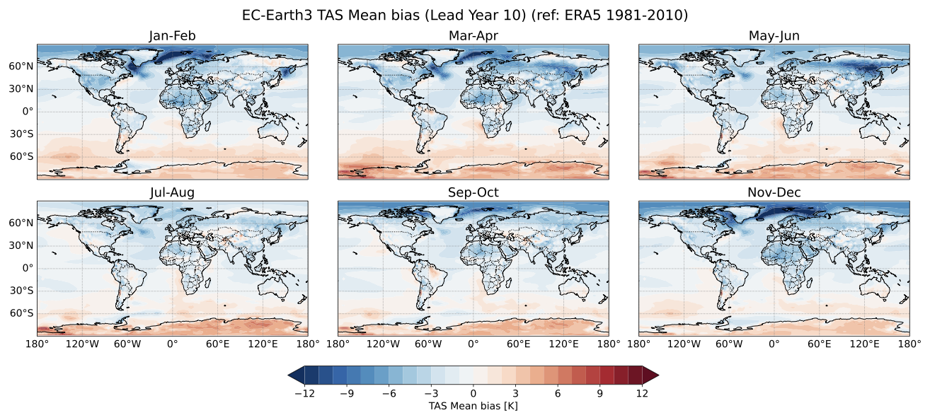
Figure 3 This example figure shows the spatial distribution of the mean bias in TAS, averaged over two-month periods, for EC-Earth3 model at LY10. All cases are available at https://pcmdi.llnl.gov/pmp-preliminary-results/graphics/dcpp/mean_bias/fig1a_interactive_TAS_mean_bias_portrait_plot.html, last access: 20 June 2026). The dataset and codes can be found in Choi and Lee (2026) and Lee et al. (2026).

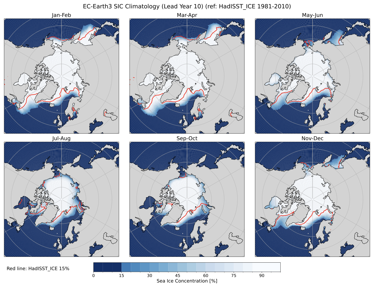
Figure 4 This example figure illustrates the spatial distribution of the climatology of Arctic sea-ice concentration, averaged over two-month periods of 1981–2010. It is shown for EC-Earth3 model at LY10. Red line represents the observed value of 15 % from HadISST_ICE for the same period. All cases are available at https://pcmdi.llnl.gov/pmp-preliminary-results/graphics/dcpp/mean_bias/fig2a_interactive_Arctic_mean_bias_portrait_plot.html, last access: 20 June 2026). The dataset and codes can be found in Choi and Lee (2026) and Lee et al. (2026).

3.2 Trend bias

Figures 5 and 6 show the long-term trend bias for the period from 1979 to 2014. During this period, a warming trend is observed in all regions except the Antarctic. The observed warming trends are as follows: Arctic 0.57, NH mid-latitudes 0.28, Tropics 0.13, and SH mid-latitudes 0.04 K per 10 years (see also Fig. S1). This latitudinal structure reasonably reflects the Arctic amplification (e.g., Smith et al., 2019; Screen et al., 2025). Most models exhibit a positive bias, indicating that they simulate a stronger warming trend. This feature is particularly pronounced in the Arctic, where some models, such as CanESM5, HadGEM3-GC31-MM, and IPSL-CM6A-LR, show an increasing positive bias with lead time (Fig. 5a). The warmer bias in the Arctic is consistently larger during the cold season than during the warm season across all models (https://pcmdi.llnl.gov/pmp-preliminary-results/graphics/dcpp/trend_bias/fig5a_interactive_TAS_trend_bias_portrait_plot.html, last access: 20 June 2026). This discrepancy between observations and models of Arctic warming trends may be due to imperfect sea ice processes and surface-albedo feedback within the models, differences in internal variability, and changes in observed trends over the analysis period (Huang et al., 2019; Ye and Messori, 2021; Chylek et al., 2023).

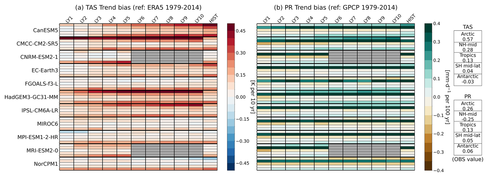
Figure 5 Same as Fig. 1, but for the trend bias over the period 1979–2014. The trend bias is defined as the difference in trend between the model and the observations. Units are [K per 10 years] for (a) TAS and [mm d⁻¹ per 100 years] for (b) PR. Trend bias is calculated for each month and each grid cell, and then annual and area averages are taken.

In contrast, observations show a very weak cooling trend over the Antarctic (−0.03 K per 10 years). This is likely because temperature trends in Antarctica are not stationary over time; rather, they are greatly influenced by inter-decadal variability in the surrounding atmosphere and ocean (Jun et al., 2020; Dalaiden et al., 2021; Sato and Simmonds, 2021). The models, however, tend to simulate a warming trend and thus show a positive bias. The Antarctic warm bias is more prominent in sea-ice regions rather than over the continent itself (see subplots at https://pcmdi.llnl.gov/pmp-preliminary-results/graphics/dcpp/trend_bias/fig5a_interactive_TAS_trend_bias_portrait_plot.html, last access: 20 June 2026). This indicates that current climate models have difficulty representing sea ice-related climate feedback and inter-decadal variability in the Antarctic region.

Trend bias in PR is most prevalent in the NH mid-latitudes for all models (Fig. 5b). Although the observed trend during this period is negative (−0.25 mm d⁻¹ per 100 years; Adler et al., 2017), all models fail to simulate the observed drying trend, even at short lead times. For instance, a significant drying trend is present in the western North Atlantic and western North America from January to February (Fig. S2). However, all models show a positive (wet) bias that exceeds the magnitude of the observed trend, even within the one-year forecast range (Fig. 7, see subplots at https://pcmdi.llnl.gov/pmp-preliminary-results/graphics/dcpp/trend_bias/fig5b_interactive_PR_trend_bias_portrait_plot.html, last access: 20 June 2026). Given the fact that the models are initialized in November or January, this suggests that relatively coarse-resolution climate models fail to capture key wintertime NH mid-latitudes precipitation processes, even within the seasonal prediction timescales. In contrast to the NH mid-latitudes, the tropics exhibit a positive observed trend (0.13 mm d⁻¹ per 100 years), yet the models demonstrate a dry bias. This bias largely results from the models' inability to reproduce the observed wetting trend over the Indian Ocean during September–December (see also the same subplots).

Observations show the strongest negative SIE trend in the Central Arctic (−12.74 × 10⁴ km² per 10 years), particularly during September–October (see subplots at https://pcmdi.llnl.gov/pmp-preliminary-results/graphics/dcpp/trend_bias/fig6a_interactive_Arctic_trend_bias_portrait_plot.html, last access: 20 June 2026). A negative annual-mean trend is also observed in the North Atlantic, particularly from November to June. The trend bias is generally negative in the North Atlantic and North Pacific, but eight out of 10 models exhibit a positive bias in the Central Arctic (Fig. 6a). Interestingly, models with strong positive biases in Arctic temperature trends, such as CMCC-CM2-SR5, HadGEM3-GC31-MM, and IPSL-CM6A-LR, also exhibit strong biases in sea-ice shrinkage trends, particularly in the North Atlantic.

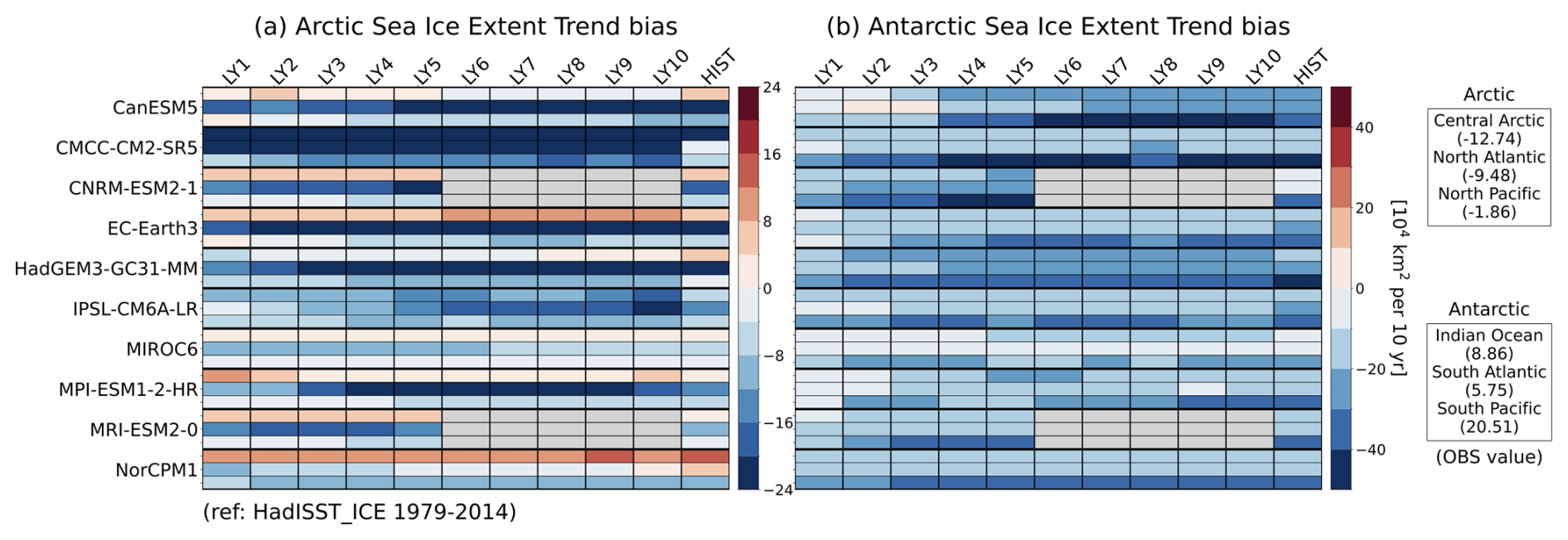
Figure 6 Same as Fig. 2, but for the trend bias of (a) the Arctic and (b) the Antarctic sea-ice extent. Units are [10⁴ km² per 10 years].

An expansion trend of SIE is observed in the Antarctic from 1979 to 2014, particularly in the South Pacific (20.51 × 10⁴ km² per 10 years) (see also contours in Fig. 8). Most models fail to reproduce this increasing trend, instead showing a negative trend bias (see also Purich et al., 2016). At shorter lead times, some models (e.g., CanESM, EC-Earth3, and MRI-ESM2-0) simulate the positive trend, resulting in a relatively small trend bias (Fig. 6b, see also subplots at https://pcmdi.llnl.gov/pmp-preliminary-results/graphics/dcpp/trend_bias/fig6b_interactive_Antarctic_trend_bias_portrait_plot.html, last access: 20 June 2026). However, as the lead time increases, the models show a transition toward a negative trend and an increase in the magnitude of the bias. These results suggest that improving sea ice initialization may enhance prediction skills, at least for shorter lead times.

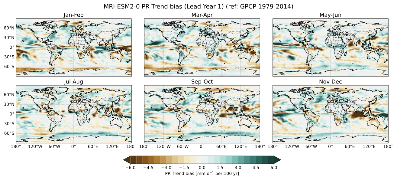
Figure 7 This example figure shows the spatial distribution of the trend bias in PR, averaged over two-month periods, for MRI-ESM2-0 model at LY1. All cases are available at https://pcmdi.llnl.gov/pmp-preliminary-results/graphics/dcpp/trend_bias/fig5b_interactive_PR_trend_bias_portrait_plot.html, last access: 20 June 2026). The dataset and codes can be found in Choi and Lee (2026) and Lee et al. (2026).

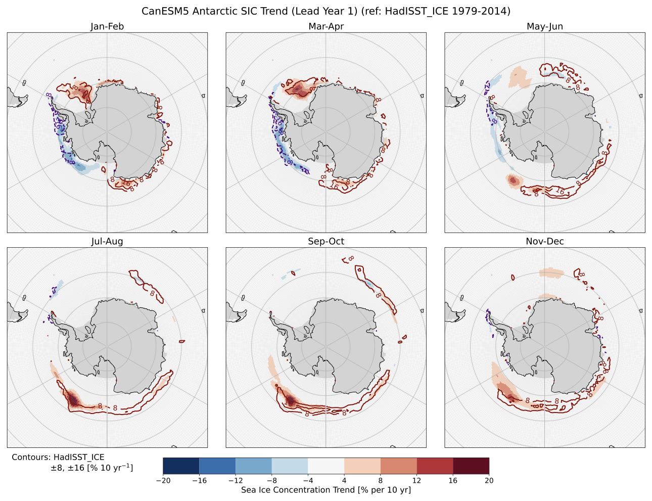
Figure 8 This example figure illustrates the spatial distribution of the trend in Antarctic sea-ice concentration, averaged over two-month periods of 1979–2014. It is shown for CMCC-CM2-SR5 model at LY1. Red (purple) lines represent the observed trend of 8 % and 16 % (−8 % and −16 %) per 10 years from HadISST_ICE for the same period. All cases are available at https://pcmdi.llnl.gov/pmp-preliminary-results/graphics/dcpp/trend_bias/fig6b_interactive_Antarctic_trend_bias_portrait_plot.html, last access: 20 June 2026). The dataset and codes can be found in Choi and Lee (2026) and Lee et al. (2026).

3.3 Skill scores

Figure 9 shows the ACC, MSSS, and RPC of the annual-mean TAS using all available initialized decadal hindcasts. These metrics are first calculated at each grid cell and then averaged over the five regions. The top row presents the MME results. For the skill scores (ACC and MSSS), the MME clearly outperforms most individual models (Fig. 9a and b). Overall, prediction skill is highest in the tropics and lowest in the Antarctic. As the ACC only considers the sign of the predicted variability, its value remains high across all lead times due to the strong warming trend. In contrast, the MSSS, which estimates the magnitude of the predicted variability in addition to the sign, drops sharply after LY1. Meanwhile, the prediction skill is enhanced for the LY1–5 prediction compared with the LY1 prediction due to the temporal smoothing, consistent with previous studies (e.g., Hermanson et al., 2022; Choi et al., 2026).

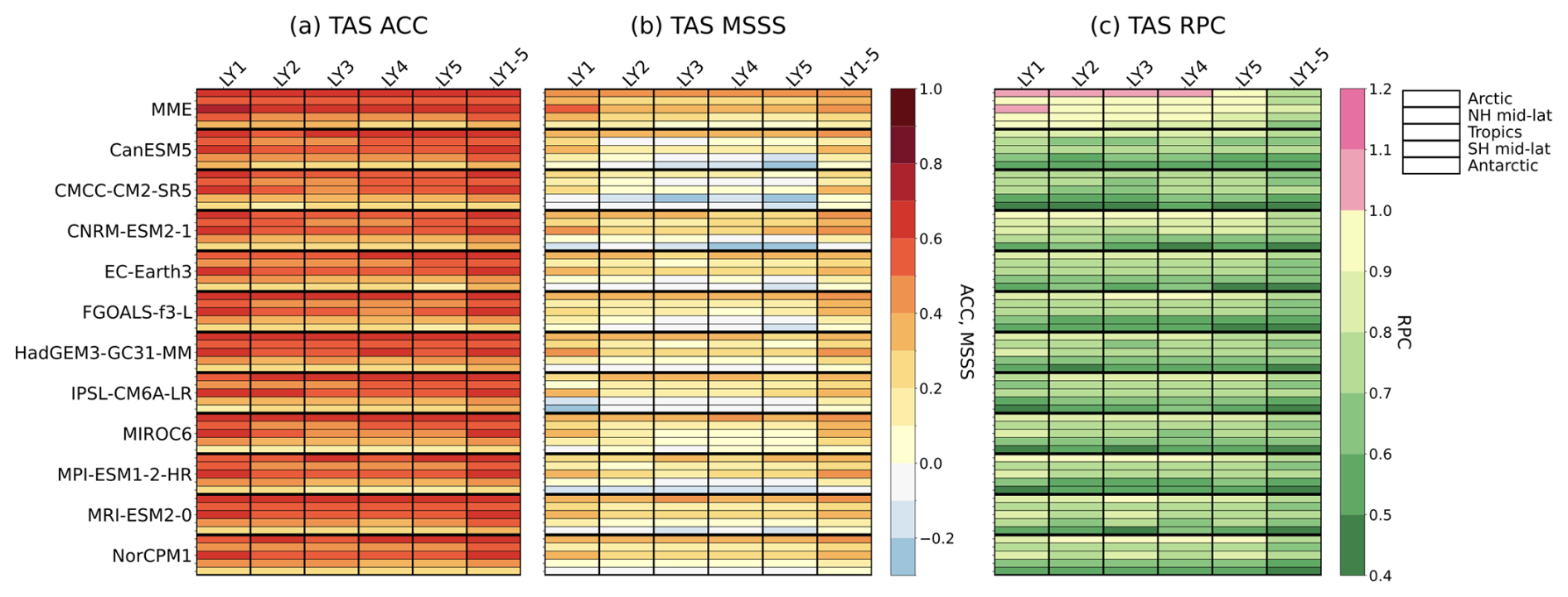
Figure 9 Model-by-lead-time portrait plot showing the (a) ACC, (b) MSSS, and (c) RPC of TAS for the multi-model ensemble mean (MME) and each model at LY1, LY2, LY3, LY4, LY5, and LY1–5. Skill scores are calculated using the annual-mean TAS at each grid cell, and then averaged across the regions. RPC is only calculated in regions where ACC > 0.

Figure 10 illustrates an example of the interactive plot for the grid-cell-based ACC of the MME at LY1. The hatched regions in Fig. 10a–c indicate areas where the ACC is below 0.6, a commonly used empirical threshold for limited practical prediction skill. ACC usually exceeds 0.6 over major ocean basins, but tends to fall below 0.6 over land and in the Southern Ocean (Fig. 10a). Since these values are influenced by initialization and external forcing, Fig. 10b–d are included to separate these effects. Figure 10b and c show the ACC from the initialized decadal hindcasts and HIST, respectively, for the same evaluation period (1965–2014) to ensure a fair comparison. The differences between Fig. 10b and c highlight the impact of initialization on the ACC (see Fig. 10d). As in previous studies, initialization has a significant impact on the skill scores in the tropical Pacific and North Atlantic regions (Meehl et al., 2016; Bilbao et al., 2021; Choi and Son, 2022). Skill enhancement in the tropical Pacific is evident in all models at LY1. Additionally, a strong effect is found near 60° S in the South Pacific. This region is dominated by long-term variability in the Antarctic deep-sea bottom waters, and improved prediction performance through initialization has been reported (Zhang et al., 2017). This can be interpreted as an improvement associated with sea ice initialization, as discussed in Fig. 6b. These enhancements are consistent across all models in the South Pacific at both LY1 and LY1–5. However, they diminish rapidly as lead time increases (see subplots at https://pcmdi.llnl.gov/pmp-preliminary-results/graphics/dcpp/skill_score/fig9a_interactive_TAS_skill_ACC_portrait_plot.html, last access: 20 June 2026).

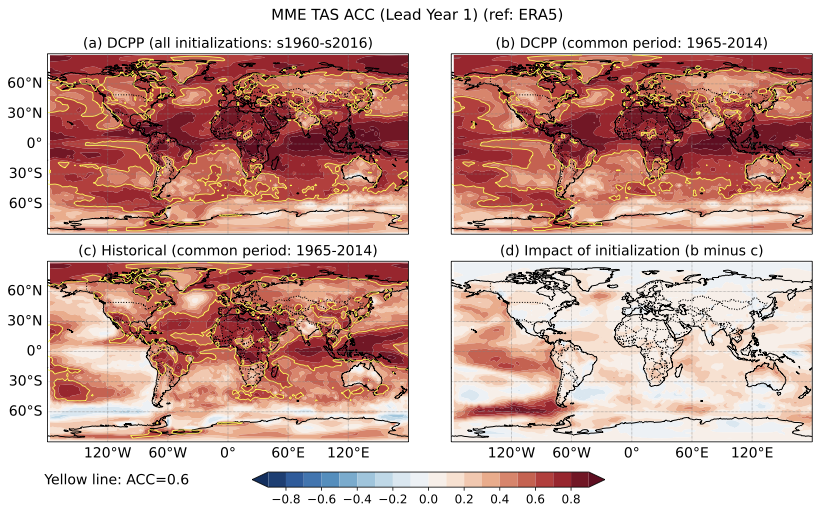
Figure 10 This example figure illustrates the spatial distribution of MME at LY1 of TAS ACC. (a) ACC calculated from all available DCPP experiments initialized from 1960 to 2016. (b) and (c) Same as (a) but for the common evaluation period of 1965–2014 from DCPP and HIST simulations, respectively. Regions with ACC below 0.6 are hatched to indicate limited practical prediction skill. (d) The difference between (b) and (c) represents the added skill due to initialization. Red regions indicate areas where initialization improves prediction skill.

Figure 9c shows the RPC values for the MME and the individual models. Most models have RPC values below one because they have fewer than ten ensemble members. In contrast, the MME, which has a total of 109 ensemble members, yields an RPC greater than one in the tropics and the Arctic. The RPCs greater than one of MME LY1 in the tropics are more prevalent in the Northern Hemisphere than in the Southern Hemisphere (Fig. 11a). In the Arctic, high RPC values appear in the Central Arctic region. However, the HIST also shows high values in the same region, suggesting that the higher RPCs in the Arctic arise from the external forcing rather than initialization. RPCs greater than one are also found in the western Antarctic; however, this is offset by small values in the eastern Antarctic through zonal-mean averaging (Fig. 9c). These high RPCs are associated with improvements in ACC due to initialization (compare Fig. 11b–d).

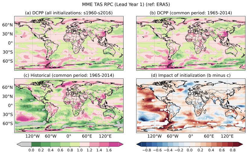
Figure 11 Same as Fig. 10 but for the RPC.

It is interesting to note that the RPC of MME at LY1–5 drops below one in most regions, even though the ACC is high at this lead time (Fig. S3a and b). Since ACC is used as the numerator in the RPC definition, the decrease in RPC is likely due to a substantial increase in the denominator, which is the predictable component of the model (see Eq. 3). In other words, this indicates that the long-term variability of individual ensemble members more closely agrees with the ensemble-mean predictions than the ensemble-mean forecasts reproduce the observed long-term variability. On the other hand, the HIST exhibits RPCs greater than one where the high ACC exists (Fig. S3c). These results suggest that the initialization enhances inter-member consistency, particularly for the LY1–5 predictions, compared to the historical experiment.

For precipitation, meaningful prediction skill exists only over the tropical Pacific at MME LY1 (Fig. S4), and no significant results emerge at longer lead times.

Figures 12 and 13 show the prediction skill of the Arctic and Antarctic SIE, as measured by ACC, MSSS, and RMSE. Overall, the Arctic SIE has a higher ACC and MSSS than the Antarctic SIE. In contrast, the RMSE is lower. Notably, the Central Arctic exhibits ACC values greater than 0.8 for MME in all lead times and for all individual models in LY1–5 (Fig. 12a). These high ACCs are attributable to the pronounced declining trend in this region, particularly in September (see also Fig. S5a). The lowest prediction skill is found in the North Pacific, even MSSS shows a negative value in the region (Fig. 12b). This is likely because the models fail to reproduce the observed fluctuations in the 1960s and 2010s (see also Fig. S5c). Although the climatological area is smaller in the North Atlantic than in the Central Arctic, RMSE is larger in the North Atlantic (Fig. 12c). This is due to errors in the spring, when the SIE is at its widest. The Central Arctic maintains its maximum area throughout the analysis period with negligible spring variability, while the North Atlantic SIE exhibits significant spring variability (Fig. S5a and b).

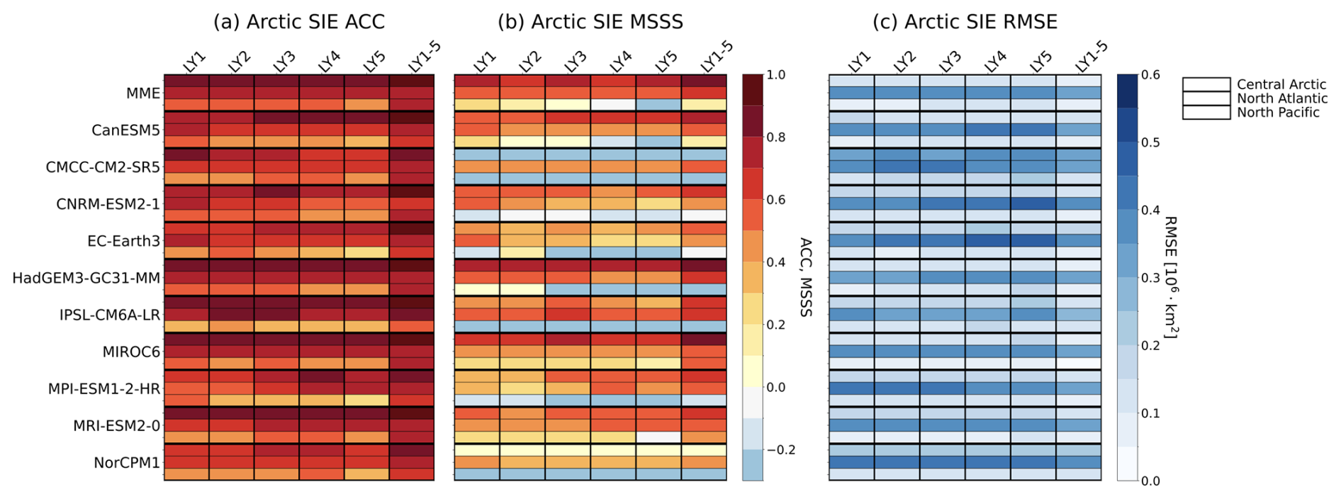
Figure 12 Model-by-lead-time portrait plot showing the Arctic SIE (a) ACC, (b) MSSS, and (c) RMSE for MME and each model at LY1, LY2, LY3, LY4, LY5, and LY1–5. SIE is first defined, and then the skill scores are calculated.

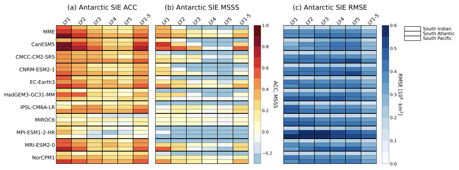
In the Antarctic, where long-term trends are much weaker than in the Arctic (see also Fig. S6), both ACC and MSSS are generally low (Fig. 13a and b). RMSE is highest in the South Pacific because its climatological extent is the largest of the three regions (Fig. 13c). Some models (e.g., CanESM5 and EC-Earth3) that realistically reproduce the positive SIE trend in the South Pacific as discussed in Figs. 6b and 8, show relatively high ACCs at LY1. Since this high ACC does not appear in the historical simulations, especially in September, it can be interpreted as an improvement due to initialization (see also Fig. S6c). A similar enhancement related to initialization is also found in the Indian Ocean in September (Fig. S6a).

Figure 13 Same as Fig. 12 but for the Antarctic SIE.

4 Summary and discussion

In this study, we introduce a comprehensive framework for evaluating and comparing the performance of multiple initialized decadal climate prediction systems using the PCMDI Metric Package. A key feature of initialized predictions, unlike the uninitialized simulations, is that both model biases and prediction skill evolve with forecast lead time. This intrinsic behaviour substantially increases the volume and complexity of evaluation results. To efficiently diagnose these characteristics, we developed two complementary visualization tools:

1. a model-by-lead-time portrait plot, which summarizes model biases and skill scores across five latitude-based regions for global temperature and precipitation, and across three sectors for the Arctic and Antarctic sea-ice extent; and

2. an HTML-based interactive visualization platform, which provides regional and seasonal diagnostics of model bias, skill scores, and ensemble spread for each model and lead time.

The portrait plots enable rapid identification of model-to-model differences and the evolution of biases and skill scores with forecast lead time. The interactive diagnostics further allow direct comparisons between initialized and uninitialized simulations, thereby helping to distinguish the relative contributions of initialization and external forcing to prediction performance.

Applying this portrait-based framework reveals several robust characteristics of decadal climate predictions. Surface air temperature biases exhibit substantial inter-model spread and a pronounced evolution with lead time, indicating a clear drift toward each model's biased climatology despite initialization. This gradual evolution likely reflects the influence of slowly varying processes associated with climate feedbacks, ocean memory, and model drift toward their preferred coupled equilibrium states. In contrast, precipitation biases show a more consistent and systematic spatial pattern across models. The relatively stable structure of these biases suggests that precipitation errors are primarily driven by higher-frequency atmospheric variability and localized convective processes that establish systematic biases early in the forecast period. This uniform structure implies common deficiencies in model physics, such as convection, cloud processes, and land–atmosphere coupling.

Trend-bias diagnostics also reveal systematic deficiencies in representing long-term climate changes regionally. Notably, the persistent underestimation of observed precipitation trends in the Northern Hemisphere mid-latitudes, even at short lead times, suggests that important mechanisms governing regional hydroclimate change may be inadequately represented in current prediction systems. These results underscore the importance of evaluating both mean-state biases and long-term trend accuracy when assessing decadal climate predictions. Finally, the results highlight the strong coupling between temperature and sea-ice predictions. Inter-model differences in sea ice extent bias generally scale with temperature bias, which emphasizes the role of polar feedback processes.

The lead-time-dependent skill diagnostics further demonstrate the distinct roles of initialization and externally forced variability in decadal prediction systems. In many regions, initialized predictions show enhanced ACC and MSSS at short lead times compared to uninitialized historical simulations, indicating the contribution of initialization to near-term prediction skills. However, this improvement often decreases with increasing lead time as internally generated variability progressively reduces the influence of the initial state. The comparison between initialized and uninitialized simulations provides a useful diagnostic framework for separating transient initialization benefits from the underlying forced climate response.

Overall, the proposed framework provides a scalable and transparent approach for multi-model evaluation and can be easily extended to future prediction systems, including CMIP Phase 7, as well as operational and research forecasting systems. In addition, future extensions of the framework should incorporate statistical significance diagnostics and uncertainty quantification for lead-time-dependent skill metrics and trend analyses. Although the present framework is primarily designed for benchmarking diagnostics rather than process-based attribution, future work should extend the framework toward process-based diagnostics that more directly connect model errors with underlying physical mechanisms.