Calibration of the MEMS v1 model over a continental soil inventory: a comparison of MCMC and 4DEnVar methods

An abundant amount of different data is required to calibrate soil organic carbon (SOC) models to represent ecosystems at large-scale. However, due to challenges related to model state projections, this calibration becomes very computationally heavy with traditional calibration methods. Here, we test 4-Dimensional Ensemble Variational data assimilation (4DEnVar) method to parameterize the MEMS v1 SOC model using data from the LUCAS network and compare its performance against MCMC calibration. Additionally, we performed an experiment where we adjusted the litter input calculation to see if the two calibration methods react differently to the change. The total SOC projections from both parameterizations showed similar improvements though the produced parameter sets differed. A thorough analysis revealed that the detailed SOC states differed from each other, but we also lacked information to determine which parameter set was closer to the truth. Furthermore, changing the litter input partition highlighted how much that assumption affects the calibration results with both methods. Our results here establish 4DEnVar as an applicable calibration method for SOC models but also highlight the need for more nuanced validation methods, as well as careful examination on how different data sets affect the model calibration.

1 Introduction

Soil organic carbon (SOC) stocks are a major component of the global carbon cycle (Scharlemann et al., 2014) and are inherently linked to surface vegetation, as the long-term SOC compounds forming them are produced by decomposition of plant litter (Cornwell et al., 2008). Due to the importance of those stocks, they are a central part of national carbon budgets (van den Berg et al., 2020) and targeted by climate related policy (e.g. LULUCF, CRCF; Schlamadinger et al., 2007) aiming at enhancing carbon accumulation into the soils and improve terrestrial carbon sinks (Rumpel et al., 2020). All of this has also highlighted the need to improve the current soil related Monitoring, Reporting and Verification (MRV) systems (Bellassen et al., 2015).

Soil inventory and numerous measurement campaigns, both temporary and continuous, have been set up to actively observe the soil carbon states within given regions and/or ecosystems (Smith et al., 2020). While these provide valuable information about the SOC stocks in that time window, also utilizing faster sample collections and analysis (Loria et al., 2024), they generally provide only information on the total SOC stocks.

To provide more nuanced SOC measurements, separating the bulk soil into SOC fractions (Cambardella and Elliot, 1992; Lavallee et al., 2020; Yu et al., 2022), notably the mineral-associated (MAOM) and the particulate organic matter carbon (POM), has been utilized more in current field campaigns. However, though there are different methods to measure these short- and long-lived SOC fractions (Delahaie et al., 2023), they require considerable resources to be applicable on a large spatial scale. Thus, models are a crucial tool in both providing more cost-effective estimates of SOC states across landscapes, as well as their responses to both climate and environmental changes.

To this purpose, numerous models of varying complexities have been developed (Chandel et al., 2023; Le Noë et al., 2023) with different approaches and focuses. Some are simple first-order dynamic models such as RothC (Coleman and Jenkins, 1996) while others are more complicated non-linear models such as MIMICS (Wieder et al., 2014) and Millennial (Abramoff et al., 2022). However, the lack of detailed information both regarding the SOC state and drivers, such as litter and soil moisture, does affect the ability to reliably constrain the various processes included into the models. Therefore, it is necessary to calibrate the model with more measurements from different pedo-climatic and land cover conditions, in order to capture how they affect the SOC state. This, though, increases the computational cost of the calibration.

Additionally complicating matters is even when using spatially diverse data for calibration, there are numerous assumptions regarding how that driver data is applied within the model that will affect not just model forward projections, but also the calibration process itself. For example, NPP is commonly used as a proxy for litterfall in SOC models (e.g. Abramoff et al., 2022; Pierson et al., 2022), with empirical work showing that the approach is justified (Matthews, 1997). How this NPP should be divided between above- and belowground biomass and, consequently between different model pools, depends on the ecosystem (Jevon et al., 2022; Cao et al., 2024) and is critical for determining the soil litter input. Without much more detailed information than is often available, these NPP/litter related parameter cannot be simultaneously calibrated with the SOC model parameters because of how fundamentally those values are connected; increasing/decreasing the amount of soil litter will simply result in an increase/decrease in decomposition rates to fit the measured SOC values. While there are valuable additional measurement datasets such as ¹⁴C (Brunmayr et al., 2024) that can provide important additional constraints for determining effective litter inputs, even these are still affected by how the NPP input is presented to start with in the model. This is just one example of driver associated assumptions and a quick nimble calibration method is needed to assess how these uncertainties impact the calibration results.

The traditional grand standard for model calibration is the Monte Carlo Markov Chain Metropolis Hastings algorithm (MCMC; Geyer, 1992). This is a very computationally heavy approach with multiple variants having been developed over the years to make it more efficient in exploring the parameter space and avoid local likelihood maximas in its search for the most likely parameter sets (e.g. Papaioannou et al., 2015; Vrugt, 2016). Due to the challenges discussed before, only computationally light SOC models can be calibrated within a practical time frame using large scale data (for example Tuomi et al., 2009). There have been workarounds presented, making assumptions about the initial state (Nemo et al., 2017; Mathers et al., 2023), using simpler calibration methods (Gurung et al., 2020) or taking advantage of machine learning approaches (Heuvelink et al., 2021). However, there remains a need for a fast and trustworthy calibration method for SOC models that would allow for easy experimentation on how different datasets affect the calibration or constraining new model dynamics being included. For example, equifinality is a known issue in ecosystem modelling, where there are multiple parameter sets that produce a similar model output (Sierra et al., 2015; Marschmann et al., 2019). Establishing if this is affecting the model system under study requires repeating the calibration multiple times which is prohibited by too heavy calibration approaches.

As a more practical alternative to the costly MCMC approach, four-dimensional ensemble variational data assimilation (4DEnVar; Liu et al., 2008) is a novel data assimilation approach, where a model ensemble generated by varying the parameters/variable states of interest is used to determine the optimal parameter and/or state variables. It has already been used for parameter calibration (Douglas et al., 2025; Pinnington et al., 2020) and is much faster than the traditional MCMC methods. It is based on the Four-dimensional Variational data assimilation (4DVar; Le Dimet and Talagrand, 1986), where a model projection is compared with observations and the new initial state for the next iteration is generated from this information. A key difference between MCMC and 4DVar based methods is that the latter use gradient descent methods to determine the next state instead of randomly sampling. While 4DVar has initially been used more commonly for state data assimilation, for example, in weather forecast (Huang et al., 2009), it has also been successfully applied to calibrate ecosystem models (e.g. Raoult et al., 2016; Peylin et al., 2016; Pinnington et al., 2016). However, to implement 4Dvar with observations from multiple different times, an adjoint version of the model is needed which imposes its own challenges and limitations on the application (Thepaut and Courtier, 1991). The 4DEnVar method uses the ensemble to sidestep this requirement by simultaneously running multiple simulations with different parameter sets instead of an iterative solution. While to our knowledge there haven't been previous studies within the ecosystem modelling analysing the performance of the 4DEnVar to that of MCMC, in Beylat et al. (2025) the 4DEnVar method is compared to the original 4DVAR method in a very specific synthetic experiment. Within that scope the 4DEnVar was shown to be more effective than the original version, but it is only the first step in evaluation.

In the work presented here, we calibrated the MEMS v1 SOC model (Robertson et al., 2019) with both MCMC and 4DEnVar parameterization methods. The model in question simulates organic carbon decomposition separately for above- and below-ground carbon with pathways from surface vegetation matter to the soil pools. In the framework of the MEMS v1, the microbial pool is the central connection between the different SOC states and, crucially, along with the soil properties regulates the amount of carbon stored as long-lived MAOM compounds. The SOC pools are for the most part connected by first order dynamics, but the relationship between the microbial and MAOM pool is non-linear. Consequently, there is only a small number of central parameters to calibrate while simultaneously the model steady state cannot be analytically solved, requiring the more costly parameterization process.

Soil data from the Land Use/Land Cover Area Frame Survey (LUCAS) measurement network (Orgiazzi et al., 2018) were used for calibration and validation against estimated model parameters, assessing their performances relative to each other and the default parameters. Because this LUCAS dataset contains measurements from thousands of plots across Europe and, thus, represents many different types of ecosystems as well as climate conditions, it allows to test a wider performance of the model calibration. One of the advantages was the level of standardisation in sample collection and analysis, the latter done by a unique laboratory, Furthermore, for a small subset of the chosen LUCAS dataset, the POM/MAOM fractioning also had been done, which provided more nuanced information for the calibration process. While Lucas is a standardised framework for SOC, was not specifically designed to assess the MAOM stocks.

Our hypothesis is that the 4DEnVar improves the model fit to a sufficient degree that, along with the reduced computational cost, it can be considered as valid calibration approach for SOC models as the MCMC. Specifically, there are two objectives for the work presented here: the first is to test if the much faster 4DEnVar calibration performs as well as the MCMC calibration and examine if there are any meaningful differences in the resulting parameter sets; the second is to conduct a simple experiment where we made a change on how the NPP litter input was partitioned. The reasoning for the latter objective is that one of the core benefits of the faster calibration method is that it allows testing how different assumptions impact the parameterizations. Because of this, if there are differences between the results of the two calibration methods, it is important to assess if the general behaviour of the parameterizations remains the same even under different assumptions.

2 Methods and data

2.1 LUCAS measurements

For the model calibration, we used the LUCAS points from a field campaign conducted in 2009 as reported in Cotrufo et al. (2019) and Lugato et al. (2021). This dataset comprises; (1) the main physico-chemical characteristic of topsoil (0–20 cm), including total SOC content for about 20 000 samples distributed across different land covers in the EU and UK; (2) a size-fraction of the bulk SOC into mineral-associated (MAOM) and particulate organic matter carbon (POM) in a representative sub-set of 350 samples. The latter were randomly drawn from the all the measurements with the only constraint being that both datasets were similarly distributed across ecosystems with approximately 73 % being grass- or croplands with the rest being various forest types. Figure 1 shows the LUCAS data points across Europe and the calculated SOC stock at each measurement site. The representativeness of the chosen 350 measurements points is elaborated upon in Lugato et al. (2021).

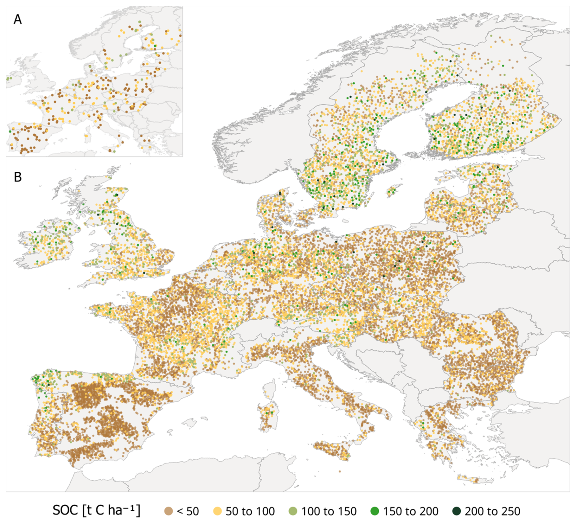
Figure 1 The LUCAS 2009 sampling points across Europe and their SOC stock used for (A) calibration and (B) validation.

For the calibration, the 348 LUCAS measurements from the 2009 campaign containing POM/MAOM fractions are used. The remaining 19 476 total SOC measurements were set aside for validation. In both allocations, measurements which were not classified as agricultural, grassland or forest were removed as well as all the sampling points where the driver data was not available. As a result, 322 datapoints are used for calibration and 17 430 for validation.

While the benefit of the LUCAS dataset is its large spatial representation and inclusion of measurements from multiple different ecosystems, the execution of such a vast measurement campaign introduces different source of errors from sampling, labelling, analysis etc. Thus, it is almost more apt to be considered as a combination of several independent campaigns done with the same protocols, instead of a single consistently controlled campaign. Additionally, although locations of the measurement are known, we have the make the assumptions that the available driver data are representative for the actual conditions at the measurement plot.

2.2 MEMS mode and parameters chosen for calibration

The Microbial Efficiency-Matrix Stabilization V1 (referred to simply as MEMS for simplicity; Robertson et al., 2019) model is a novel soil organic carbon (SOC) model framework, which is built around the scientific understanding that the soil microbial pool modulates the SOC stocks. The model structure is presented in Fig. S1 in the Supplement. In the model, both surface vegetation and SOC decomposition are represented by multiple pools defined by their physical properties. There are several paths for carbon fluxes to transfer from one pool to another or lost as CO₂, with the rate of change calculated on a daily timestep. The model dynamics represents the depth of the soil measurements used to calibrate it. As we are using the LUCAS data here which is from the top 20 cm of the soil, the resulting MEMS model will thus simulate the SOC dynamics of top 20 cm layer as well.

Since the parameterization focuses on the SOC stock, only the model equations affecting MEMS pools C5 (Heavy particulate organic matter), C8 (Dissolved organic matter), C9 (Mineral associated organic matter (MAOM)) and C10 (Light particulate organic matter) were calibrated here. The vegetation decomposition pools C1 (hot-water soluble), C2 (acid soluble) and C3 (acid insoluble) as well as the surface microbial pool (C4) and the dissolved organic matter (C6) do determine the litter input entering to soil C pools. These mechanics were not included in the calibration as the type of data required to constrain them was not available. Therefore, we used the default parameters values established in Robertson et al. (2019) for the surface processes since they had been chosen to be representative of the LUCAS network environment. Meanwhile the released CO₂ (C7) and the leached dissolved material to the soil (C11) are cumulative removal pools and do not have any parameters to be calibrated.

The equations that govern the change in the relevant pools in MEMS are:

$$\begin{array}{}\text{(1)}& {\displaystyle \frac{\mathrm{d}{C}_{\mathrm{5}}}{\mathrm{d}t}}=C_{\mathrm{5},\mathrm{in}}^{\mathrm{2}}+C_{\mathrm{5},\mathrm{in}}^{\mathrm{3}}+C_{\mathrm{5},\mathrm{in}}^{\mathrm{4}}-T_{\mathrm{mod}}{k}_{\mathrm{5}}{C}_{\mathrm{5}}\text{(2)}& {\displaystyle }\begin{array}{rl}{\displaystyle \frac{\mathrm{d}{C}_{\mathrm{8}}}{\mathrm{d}t}}& =C_{\mathrm{8},\mathrm{in}}^{\mathrm{5}}+C_{\mathrm{8},\mathrm{in}}^{\mathrm{6}}+C_{\mathrm{8},\mathrm{in}}^{\mathrm{10}}-\mathrm{sorp}-{\mathrm{DOC}}_{\mathrm{lch}}{C}_{\mathrm{8}}\\ & -T_{\mathrm{mod}}{k}_{\mathrm{8}}{C}_{\mathrm{8}}\end{array}\text{(3)}& {\displaystyle \frac{\mathrm{d}{C}_{\mathrm{9}}}{\mathrm{d}t}}=\mathrm{sorp}-T_{\mathrm{mod}}{k}_{\mathrm{9}}{C}_{\mathrm{9}}\text{(4)}& {\displaystyle \frac{\mathrm{d}{C}_{\mathrm{10}}}{\mathrm{d}t}}=C_{\mathrm{10},\mathrm{in}}^{\mathrm{2}}+C_{\mathrm{10},\mathrm{in}}^{\mathrm{3}}-T_{\mathrm{mod}}{k}_{\mathrm{10}}{C}_{\mathrm{10}}\end{array}$$

Where C_i is the amount of carbon stored in pool i, $C_{i,\mathrm{in}}^j$ is the carbon input to pool i from pool j as a result of the decomposition process and k_i is the decomposition rate for pool i. The leaching coefficient DOC_lch represents the dissolution of SOC to deeper soil layers and the temperature coefficient T_mod reflects how soil temperature affects the decomposition rate. In this work, T_mod is the same for all pools and follows the STANDCARB 2.0 model (Harmon et al., 2009) which is an expanded version of the traditional Q10 temperature model where the limiting impact of the high temperatures is accounted for.

The sorption coefficient sorp controls the flow of carbon between the microbial pool and the mineral associated carbon pool as determined by the equation

$$\begin{array}{}\text{(5)}& {\displaystyle }\mathrm{sorp}=C_{\mathrm{8}}{\displaystyle \frac{\frac{K_{\mathrm{lm}}{Q}_{\max }{C}_{\mathrm{8}}}{\mathrm{1}+K_{\mathrm{lm}}{C}_{\mathrm{8}}}-C_{\mathrm{9}}}{Q_{\max }}}\text{(6)}& {\displaystyle }{Q}_{\max }=d\cdot {\mathit{\rho }}_{\mathrm{soil}}\cdot \left(\mathrm{1}-p_{\mathrm{rock}}\right)\cdot {\mathrm{sc}}_{\mathrm{Conc}}\text{(7)}& {\displaystyle }{\mathrm{sc}}_{\mathrm{conc}}={\mathrm{sc}}_{\mathrm{slope}}\cdot \left(\mathrm{1}-p_{\mathrm{sand}}\right)+{\mathrm{sc}}_{\mathrm{int}}\end{array}$$

In which K_lm is the langmuir isotherm term that depends on the soil pH, Q_max is the maximum absorption capacity of the soil, ρ_soil is the soil bulk density, p_rock is the rock percentage of the soil and p_sand is the sand percentage of the soil. The maximum concentration of fine fraction, sc_conc, is governed by the two coefficients sc_int and sc_slope. Consequently, those two parameters effectively control the saturation ratio for the MAOM pool.

The decomposition rate parameters k₅, k₈, k₉ and k₁₀ were the central parameters chosen for calibration as well as sc_int and sc_slope. As the primary focus of this work is to compare the calibration methods, these parameters were simply chosen as a straight-forward test case. The boundary values are presented in Table 1. As will explained in Sect. 2.5, we do need an expected value for these parameters in order to create a prior uncertainty distribution. We chose this value by randomly drawing a parameter value from near the middle of the set of the boundary conditions after testing that the model runs remained stable with these parameter values.

Table 1 The calibrated parameters chosen for calibration, their assigned expected parameter values as well as boundaries that constrain the lowest and highest values that the parameters are allowed be given during the calibration.

To determine how we divide the litter input to MEMS model pools, the site ecosystem type was assigned by the Corine Land Cover (Buttner, 2014). Following that, NPP is split into the MEMS model pools according to the following framework established in Robertson et al. (2019):

$$\begin{array}{}\text{(8)}& {\displaystyle }{C}_{\mathrm{1},\mathrm{input}}\left(t\right)=\left(\mathrm{1}-f_{\mathrm{doc}}^{\mathrm{eco}}\right)f_{\mathrm{sol}}^{\mathrm{eco}}{r}^{\mathrm{eco}}\mathrm{NPP}\left(t\right)\text{(9)}& {\displaystyle }{C}_{\mathrm{2},\mathrm{input}}\left(t\right)=\left(\mathrm{1}-f_{\mathrm{sol}}^{\mathrm{eco}}-f_{\mathrm{lig}}^{\mathrm{eco}}\right)r^{\mathrm{eco}}\mathrm{NPP}\left(t\right)\text{(10)}& {\displaystyle }{C}_{\mathrm{3},\mathrm{input}}\left(t\right)=f_{\mathrm{lig}}^{\mathrm{eco}}{r}^{\mathrm{eco}}\mathrm{NPP}\left(t\right)\text{(11)}& {\displaystyle }{C}_{\mathrm{6},\mathrm{input}}\left(t\right)=f_{\mathrm{sol}}^{\mathrm{eco}}{f}_{\mathrm{doc}}^{\mathrm{eco}}{r}^{\mathrm{eco}}\mathrm{NPP}\left(t\right)\end{array}$$

Where C_i,input(t) is the carbon input to pool i from NPP at a given time t and eco refers to the ecosystem for the LUCAS point. Then, f_sol is the hot water extractable fraction of the litter input, f_doc is the cold-water extractable fraction of the water extractable fraction and f_lig is the acid-insoluble fraction of the of the litter input. It is important to note that these fractions are not the totality of the litter input and, while equations from 8 to 11 do sum up to the total NPP, the fractions presented here do not sum up to 1. Finally, the r^eco represents the fraction of NPP that is assumed to have been removed from the system due to economic activies (harvest, grazing, etc.)

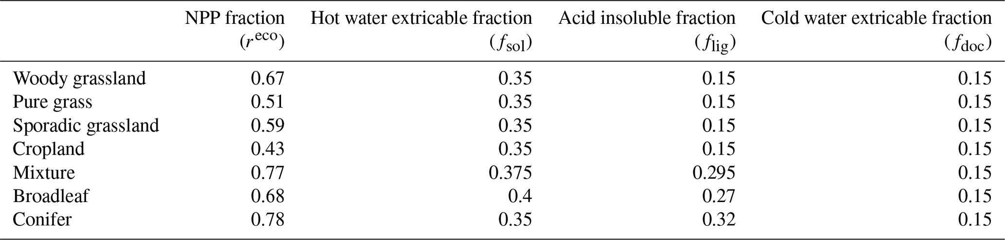
The coefficient values based on Campbell et al. (2016) are presented in Table 2. It is important to make two notes regarding these values. First, we are using a single fraction here and do not account for the uncertainty range provided in the work referenced. Second, only f_sol and f_lig fraction ranges are presented in Campbell et al. (2016). For f_doc we used a constant value across land covers in line with the work Robertson et al. (2019).

Table 2 The fraction of NPP that is used for litter input and how it is divided into different litter compounds.

2.3 MCMC

Markov Chain Monte Carlo (MCMC; Geyer, 1992) is a widely used Bayesian model parameterization method. The basis of this approach is straightforward: First values for the parameters chosen for calibration are drawn by randomly perturbing accepted parameter values and the model is run for given locations with these parameters. Assuming that the uncertainties are normally distributed, the total likelihood F of these projections, given observations that correspond to model predictions, is calculated with

$$\begin{array}{}\text{(12)}& \begin{array}{rl}F& ={\prod }_{l=\mathrm{1}}^{N_{\mathrm{obs}}}{\left(\mathrm{2}\mathit{\pi }{\mathit{\sigma }}_l^{\mathrm{2}}\right)}^{\frac{\mathrm{1}}{\mathrm{2}}}{e}^{-\frac{\mathrm{1}}{\mathrm{2}}{\sum }_{l=\mathrm{1}}^{N_{\mathrm{obs}}}\frac{{\left(x_l-y_l\right)}^{\mathrm{2}}}{{\mathit{\sigma }}_l}}\\ & \cdot {\prod }_{k=\mathrm{1}}^{N_{\mathrm{par}}}{\left(\mathrm{2}\mathit{\pi }{\mathit{\sigma }}_{\mathit{\theta },k}^{\mathrm{2}}\right)}^{\frac{\mathrm{1}}{\mathrm{2}}}{e}^{-\frac{\mathrm{1}}{\mathrm{2}}{\sum }_{l=\mathrm{1}}^{N_{\mathrm{par}}}\frac{{\left({\mathit{\theta }}_k-{\mathit{\theta }}_{k,\mathrm{prior}}\right)}^{\mathrm{2}}}{{\mathit{\sigma }}_{\mathit{\theta },k}}}\end{array}\end{array}$$

Where l is the observation index, N_obs is the number of observations, σ is the associated uncertainty, x_l is the model projection with parameter set θ and y_l is the observation for index l. Furthermore, k is the parameter index, N_par is the number of parameters being estimated and Θ_prior is the prior estimate of parameters.

Once the likelihood is determined, it is compared to the likelihood of the previously accepted parameter set. If the new likelihood is higher, then that parameter set is automatically accepted and used as the parameters for the next iteration. However, if the new likelihood is lower than the previous one, there is still a probability that the new parameter set will still be accepted depending on how close the new likelihood is to the previous accepted likelihood.

By allowing the lower likelihoods to be possibly accepted, MCMC also provides an acceptable parameter range, which can be used to represent the parameter uncertainties. This iterative process is repeated until a given convergence goal is satisfied (Roy, 2020).

For the study here, we used the MCMC framework established in Viskari et al. (2022), which utilizes the BayesianTools R-library (Hartig et al., 2019). The chosen MCMC algorithm is the Differential evolution Markov Chain with snooker updater (DEzs; ter Braak and Vrugt, 2008), where multiple calibration chains progress concurrently from different starting point with information shared between the chains at given intervals. This should lead to a more efficient and faster convergence of the calibration, especially as this approach makes it possible to parallelize the different chains.

Six chains were used for the calibration with the initial values for each chain randomly drawn from the prior parameter range. The MCMC was run for 100 000 accepted iterations with the convergence test and statistical values calculated from the last 10 000 iterations.

2.4 4-Dimensional Ensemble Variational assimilation

Instead of iteratively exploring the variable space like MCMC does, 4-Dimensional Ensemble Variational data assimilation (4DEnVar) uses an ensemble of model runs with different variable sets and that are independent of each other. The ensemble of model runs is used to approximate information required by other calibration techniques, such as the gradient of the cost function and a mapping from variable space to observation space. Because there is no need for a large amount of model run repetitions such as in MCMC, this method is a computationally much faster. However, this approach is built on certain assumptions – in particular that the observations can be predicted by a linear combination of the different ensemble members – which make it important to test before-hand how well it is able to find the correct values in different systems.

The foundational theory for the 4DEnVar method is explained in Liu et al. (2008). The formulation established in Pinnington et al. (2020) was used as the basis for this work. In this section, we will provide a simplified description of the method as it applies to our purposes.

In traditional baseline 4-Dimensional Variational data assimilation (4DVar; Le Dimet and Talagrand, 1986), similarly to MCMC, the most likely state, i.e. the model parameter set, is solved by determining the minimum of the cost function J

$$\begin{array}{}\text{(13)}& \begin{array}{rl}J& ={\displaystyle \frac{\mathrm{1}}{\mathrm{2}}}({\left(\mathit{\theta }-{\mathit{\theta }}_{\mathrm{prior}}\right)}^T{\mathbf{B}}^{-\mathrm{1}}\left(\mathit{\theta }-{\mathit{\theta }}_{\mathrm{prior}}\right)\\ & +\sum _{t=\mathrm{1}}^K{\left(M_{\mathrm{0}\to t}(\mathit{\theta },{\mathit{x}}_{\mathrm{0}})-{\mathit{y}}_k\right)}^T{\mathbf{R}}_t^{-\mathrm{1}}\left(M_{\mathrm{0}\to t}(\mathit{\theta },{\mathit{x}}_{\mathrm{0}})-{\mathit{y}}_k\right))\end{array}\end{array}$$

In which θ and θ_prior are, respectively, the suggested and prior parameter value vectors, B is the prior parameter error covariance matrix and R_t is the observation error covariance matrix at the measurement time t. The model operator M_0→t calculates from the given parameters and the initial state x₀ the output comparable to the observation vector y_k. The measurement times in the chosen time window is represented by K.

Two brief notes on this formulation. First, it is essentially the same as exponent component in Eq. (12), except that is written it in vector form. Second, in an effort to simplify the equations, we did not include an observation operator component in the equations. All our observations are point measurements that can be directly compared with the model output, hence a separate observation operator was unnecessary for our purposes.

4DVar, like MCMC, is also an iterative approach that calculates the cost function with different state vectors to test if the cost function value decreases. However, with 4DVar, the iterations suggested after the first attempt are not randomly drawn, but rather determined by the gradient function

$$\begin{array}{}\text{(14)}& \begin{array}{rl}\mathrm{\nabla }J& ={\mathbf{B}}^{-\mathrm{1}}\left(\mathit{\theta }-{\mathit{\theta }}_{\mathrm{prior}}\right)\\ & +\sum _{t=\mathrm{1}}^K{\mathbf{M}}_{\mathrm{0}\to t}^T{\mathbf{R}}_t^{-\mathrm{1}}\left(M_{\mathrm{0}\to t}(\mathit{\theta },{\mathit{x}}_{\mathrm{0}})-{\mathit{y}}_k\right)\end{array}\end{array}$$

Where ${\mathbf{M}}_{\mathrm{0}\to t}^T$ is the adjoint of the tangent-linear version M_0→t of the model operator M.

The benefit of the gradient use is that it results in a value of zero for the state vector that produces the cost function minimum. Thus, gradient descent techniques (Ruder, 2016) are able to use the information from the gradient to efficiently locate the cost function minimum and the optimal state vector.

Naturally, there are challenges in applying this method. The core hurdle is the adjoint operator in equation Eq. (14), which is the transpose of the tangent-linear version of process model. Creating these model versions, though, is not a simple task and imposes a linearity assumption on the driving processes. Furthermore, since background error covariance matrix B can have non-diagonal terms representing error covariances, the inverse matrix can become computationally implausible to be calculated for larger systems.

In 4DEnVar, these issues are approached by expanding on the square root transform framework established in Tippett et al. (2003). Let us have an ensemble of model runs where, in our case, every ensemble has a different parameter set randomly drawn from the same baseline prior distribution. In the 4DEnVar formulation, this prior distribution is assumed normally distributed. For each ensemble member, we can then determine how its output differs from the prior parameter set output. These perturbations from the mean across the ensemble can be written in matrix format ${\mathbf{\Theta }}_b^{\prime }$ as follows

$$\begin{array}{}\text{(15)}& {\mathbf{\Theta }}_b^{\prime }={\displaystyle \frac{({\mathit{\theta }}^{b,\mathrm{1}}-{\stackrel{\mathrm{‾}}{\mathit{\theta }}}^b,{\mathit{\theta }}^{b,\mathrm{2}}-{\stackrel{\mathrm{‾}}{\mathit{\theta }}}^b,{\mathit{\theta }}^{b,\mathrm{3}}-{\stackrel{\mathrm{‾}}{\mathit{\theta }}}^b,\mathrm{\dots },{\mathit{\theta }}^{b,L}-{\stackrel{\mathrm{‾}}{\mathit{\theta }}}^b)}{\sqrt{L-\mathrm{1}}}}\end{array}$$

Where L is the ensemble size, θ^b,i is the ith vector of the perturbation matrix, and ${\stackrel{\mathrm{‾}}{\mathit{\theta }}}^b$ is the average over the perturbations. In our case, the average over the perturbations is the same as the prior parameter vector θ_prior.

Since this matrix essentially represents the uncertainty related to the parameter values, the prior error covariance matrix B can be approximated as

$$\begin{array}{}\text{(16)}& \mathbf{B}\approx {\mathbf{\Theta }}_b^{\prime }{\mathbf{\Theta }}_b^{\prime ,T}\end{array}$$

We admit that in this formulation we ignore model structural error and assume the dominant error is from the parameter uncertainty.

Furthermore, we can define a vector w with the length of L that satisfies the equation

$$\begin{array}{}\text{(17)}& \mathit{w}={\mathbf{\Theta }}_b^{\prime ,-\mathrm{1}}\left(\mathit{\theta }-{\mathit{\theta }}_{\mathrm{prior}}\right)\end{array}$$

With these formulations and assumptions, the cost and gradient functions can be written as

$$\begin{array}{}\text{(18)}& {\displaystyle }\begin{array}{rl}\mathbf{J}\left(\mathit{w}\right)& ={\displaystyle \frac{\mathrm{1}}{\mathrm{2}}}\mathit{w}{\mathit{w}}^T\\ & +{\displaystyle \frac{\mathrm{1}}{\mathrm{2}}}\sum _{t=\mathrm{1}}^K{\left({\mathbf{M}}_{\mathrm{0}\to t}{\mathbf{\Theta }}_b^{\prime }\mathit{w}+M_{\mathrm{0}\to t}(\mathit{\theta },{\mathit{x}}_{\mathrm{0}})-{\mathit{y}}_k\right)}^T\\ & \cdot {\mathbf{R}}_t^{-\mathrm{1}}\left({\mathbf{M}}_{\mathrm{0}\to t}{\mathbf{\Theta }}_b^{\prime }\mathit{w}+M_{\mathrm{0}\to t}(\mathit{\theta },{\mathit{x}}_{\mathrm{0}})-{\mathit{y}}_k\right)\end{array}\text{(19)}& {\displaystyle }\begin{array}{rl}\mathrm{\nabla }J\left(\mathit{w}\right)& =\mathit{w}+\sum _{t=\mathrm{1}}^K{\mathbf{\Theta }}_b^{\prime ,T}{\mathbf{M}}_{\mathrm{0}\to t}^T\\ & \cdot {\mathbf{R}}_t^{-\mathrm{1}}\left({\mathbf{M}}_{\mathrm{0}\to t}{\mathbf{\Theta }}_b^{\prime }\mathit{w}+M_{\mathrm{0}\to t}(\mathit{\theta },{\mathit{x}}_{\mathrm{0}})-{\mathit{y}}_k\right)\end{array}\end{array}$$

With this new formulation, we can further approximate

$$\begin{array}{}\text{(20)}& \begin{array}{rl}\mathrm{\nabla }J\left(\mathit{w}\right)& =\mathit{w}+\sum _{t=\mathrm{1}}^K{\left({\mathbf{M}}_{\mathrm{0}\to t}{\mathbf{\Theta }}_b^{\prime }\right)}^T\\ & \cdot {\mathbf{R}}_t^{-\mathrm{1}}\left({\mathbf{M}}_{\mathrm{0}\to t}{\mathbf{\Theta }}_b^{\prime }\mathit{w}+M_{\mathrm{0}\to t}(\mathit{\theta },{\mathit{x}}_{\mathrm{0}})-{\mathit{y}}_k\right)\end{array}\end{array}$$

This formulation removes the need for the adjoint version of the model. An additional benefit of the 4DEnVar method is that the gradient function value can be calculated for each ensemble member, since we are already running an ensemble to approximate the prior error covariance matrix. This information, then, makes straightforward determining the state estimate.

Compared to filter-based data assimilation methods (for example the Ensemble Kalman Filter; Evensen, 2003), the variational methods do not estimate the posterior uncertainty directly. However, we used the method established in Pinnington et al. (2021) to calculate the posterior distributions.

For the study here, we used the 4DEnVar algorithm provided in Quaife (2023). The gradient approach method used there is BFGS2 (Saito and Nakano, 1997) from the GNU Scientific Library (GSL).

The 4DEnVar methodology holds crucial benefits for our model calibration even beyond the reduction in computational cost compared to MCMC. Even though all the measurements used for calibration in this work are from the same year, the model outputs are steady state products that take hundreds of simulated years to produce. Hence, a 3-dimensional variational data assimilation (3DVar; Lorenc et al., 2000) cannot be applied and the adjoint of the model would be required, as the gradient function needs to be calculated at the start of the simulation. To complicate things further, the validity of the tangent-linear assumption would be questionable due to the length of the simulation in this situation.

2.5 Calibration setup and uncertainty attribution

After having set up the algorithmic framework for both calibration methods for the selected LUCAS data points, the first task was to complete twin experiments. In those, we randomly drew a value for each the parameter chosen for calibration from the uncertainty distributions assigned for them in Table 1. Synthetic observations were generated with the model using the new parameter set. Then, we performed the calibration with both tested methods using these synthetic observations with their associated uncertainties set to be 1 % of those synthetic observations and still using the same prior distribution established in Table 1. This allows us to check if both methods were able to find the correct parameter sets in a situation where the true answer was known. For the 4DEnVar, the additional importance of these tests is to assess the ensemble size dimension required to consistently estimate the correct parameter set. This was accomplished by repeating the twin experiment multiple times with different ensemble sizes and choosing the ensemble size where the calibration always found the correct parameter set. The repetitions were necessary because the 4DEnVar ensemble members are randomly drawn, therefore there are potential situations where a given ensemble size can retrieve the correct parameter set several times in a row, but then fails on the next time.

After the twin experiments have been conducted, the calibration itself is performed with the calibration dataset, before the validation runs are done for the validation dataset locations. In both situations the SOC is assumed to reflect a steady state. It should be noted that with agricultural soils and commercial forests are expected to have a large variability in litter input over a given time window, which does raise challenges for the steady state approach. We are still including those data points in the analysis here as this is intended as a general calibration across European ecosystems and there is no additional data to constrain those specific ecosystems, but this is expected to be an additional uncertainty source. As a part of the testing here, we also wished to experiment how varying assumptions regarding model drivers affected the potential differences between the calibration results. For our test case study on the impact of the NPP assumptions on the parameterization, we repeated the calibrations with a small adjustment. We changed the f_doc value of grass- and croplands from 0.15 to 0.35. This increases the amount of the litter that is directly deposited to the soil and consequently adsorbed by the mineral matrix instead of being lost during the transition between the surface and soil carbon pools. In our expert opinion, there is a higher proportion of exudates and root litter (i.e. low molecule weight compounds that can directly sorbed by the soil minerals) entering the topsoil in grasslands and herbaceous compared to forests. Thus, this change is suitable for a plausible change to the NPP assumptions and makes an ideal test study to see how it affects the parameterization results and if the system depicted by the parameterizations still remains consistent after the potential change.

When calculating the steady state, the MEMS model is simulated over the period of 700 years from an initial state vector (Table S1 in the Supplement). Here, during calibration each LUCAS point is simulated for 700 years with the last output values compared to the measurements. At some sites, the MEMS model did not reach full steady state during this time, but the difference was within fractions of a percentage of the final steady state. As the change was so marginal already at this point, the shorter time period was chosen for computational efficiency.

As driver data at the European level, the model uses daily air temperature extracted from the E-OBS grid (Cornes et al., 2018). For each day of the year, an average temperature is calculated from a time series that spans from 2009–2018, with the temperature cycle then repeated for each year when calculating the steady state. Furthermore, the clay, sand and rock content of the soil as well as the soil bulk density and pH from LUCAS are used to determine soil properties driving SOC processes.

For Net Primary Production (NPP), first the average annual NPP over the decade 2000–2010 is extracted from the MODIS product MOD17A3 (Running et al., 2004) grid cell overlaying each LUCAS point. Then, a standard sine function is used to distribute the NPP across the year in order to produce the daily litter input. This approach was used instead of an averaged MODIS NPP annual time series as the NPP reflects the time when the atmospheric carbon is allocated into vegetation, not when the vegetation becomes litter input. Hence, we simplified the time series here and, since the total annual NPP remains the same, it is not expected to affect the modelling results to a notable degree.

The total SOC measurement uncertainties from the LUCAS dataset are used as the uncertainties in this application. Since LUCAS protocol requires to take a composite soil sample (out of 5 samples), the uncertainty was estimated propagating the error associated to all variables for calculating SOC stock (i.e. SOC content, depth, rock fragment). We run a Monte Carlo simulation with 5000 draws, using a standard deviation derived from the coefficient of variation reported in Goidts et al. (2009) for the microsite scale, with a similar sampling scheme of LUCAS. It is important to note, though, that these values are calculated from mixed samples. Thus, it may be an underestimation of the real uncertainty for several reasons as, for example, how LUCAS samples are overall representative of the field conditions. However, we do not have more information concerning the SOC measurement uncertainties available.

Regarding the MAOM fraction, there is no established uncertainty estimate to utilize. Because of that, we assigned an uncertainty where the standard deviation was 5 % of the measured MAOM value. This choice was driven by both a discussion with the data collection team about the reliability of the data and to ensure an appropriate weight during the calibration process. When the initial cost function is calculated using the baseline MEMS parameter set with this uncertainty, the total SOC values account for approximately two thirds of the cost function value, with the MAOM fraction being responsible for the remainder.

The prior uncertainty assigned to the parameters introduced challenges in this work. With MCMC, because we only use the prior parameter value range for the initial sampling, we were able to apply a uniform uncertainty distribution that was used to approximate the baseline parameter set from Robertson et al. (2019). For those parameters where the uncertainty was not provided, we approximated a wide enough uniform distribution around the assigned parameter value. The 4DEnVar method, though, requires a Gaussian uncertainty distribution as explained in Sect. 2.4. As there is no prior information available, we used the baseline parameter values as the expected values, with the uncertainty represented by a standard deviation of 10 % of the parameter value. This uncertainty range, deliberately imposing a larger uncertainty, resulted in 4DEnVar calibration producing negative parameter values, which are naturally unrealistic. We will discuss the reasons and implications of this behaviour later.

In some studies, for example, uncertainty has also been a parameter estimated with MCMC (Cailleret et al., 2020). Considering the meaningful unknowns regarding the uncertainty approximations, this would be a valid approach to be applied here. We did not estimate uncertainties for the initial MCMC/4DEnVar comparison, as varying the uncertainties might cause issues with the gradient approach methods and, consequently, would make it difficult to interpret the differences between the two. After the comparison, though, we did perform a MCMC calibration of MEMS, where we also estimated a scaling parameter for both total SOC and MAOM fraction uncertainties. However, these results are not shown here, as the calibration did not result in a successful convergence.

3 Results

The twin experiments (not shown) established that both methods were able to produce the true parameters when calibrating against synthetic observations. For 4DEnVar, the experiments established that an ensemble size of 250 members consistently produced the parameters used to generate the synthetic observations for all repetitions of the twin experiment and, thus, we chose this ensemble size for the 4DEnVar consequents.

Table 3 The statistically likeliest parameter values produced by the different calibration methods. The first value is for f_doc 0.15, the second for f_doc 0.35.

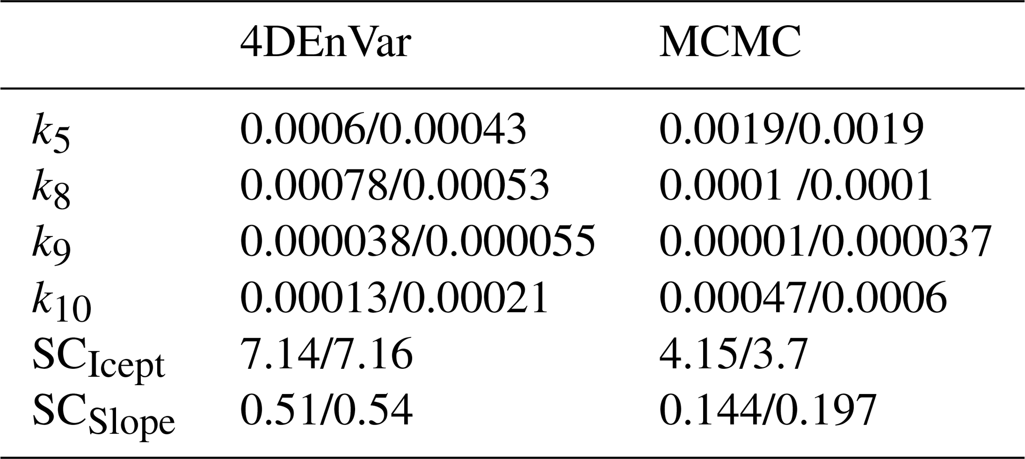
The parameter distributions estimated by the MCMC and 4DEnVar calibration for both f_doc scenarios are presented in Fig. 2. For clarity, the statistically likeliest parameter values from all the calibrations are in Table 3 and the standard deviations for the distributions in Table S2. From these, we see that MCMC and 4DEnVar parameter sets differ from each other more than explained by their associated uncertainties, but remain within the same range even when changing the NPP assumption. Furthermore, with the higher f_doc value, the parameter distributions produced by 4DEnVar remain approximately as wide even when they shift. Meanwhile with the MCMC calibration it produces wider distributions which represents larger uncertainties. It is also apparent that with three parameters (k₈, k₉ and Sc_slope), the MCMC produces expected values that are very close to the set boundaries when f_doc is set to 0.15 while, when set to 0.35, those distributions are clearly within the given parameter ranges. This indicates that with the lower f_doc, the MCMC calibration struggles to find an acceptable parameter set within the accepted range. Similarly, the uncertainties with the 4DEnVar are quite wide, which implies that it also cannot effectively locate an ideal parameter set.

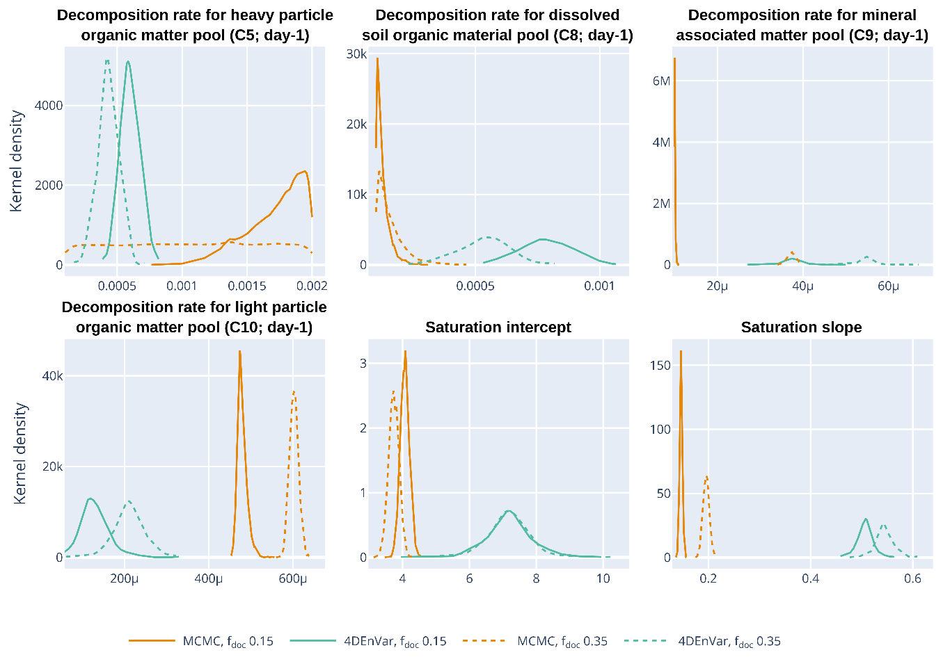
Figure 2 Estimated parameter distributions for both MCMC (orange) and 4DEnVar (green) calibrations with f_doc set to 0.15 (solid) and 0.35 (dashed). The μ indicates a multiplier of 10⁻⁶.

The uncertainty distributions for 4DEnVar are generally wider than for MCMC in both cases. With 4DEnVar, we repeated the calibration multiple times to ascertain that the randomness associated with the ensemble selection did not result in statistically different parameter sets. While there was variance in the produced parameter sets, they overall remained within the uncertainty distribution for any single estimation.

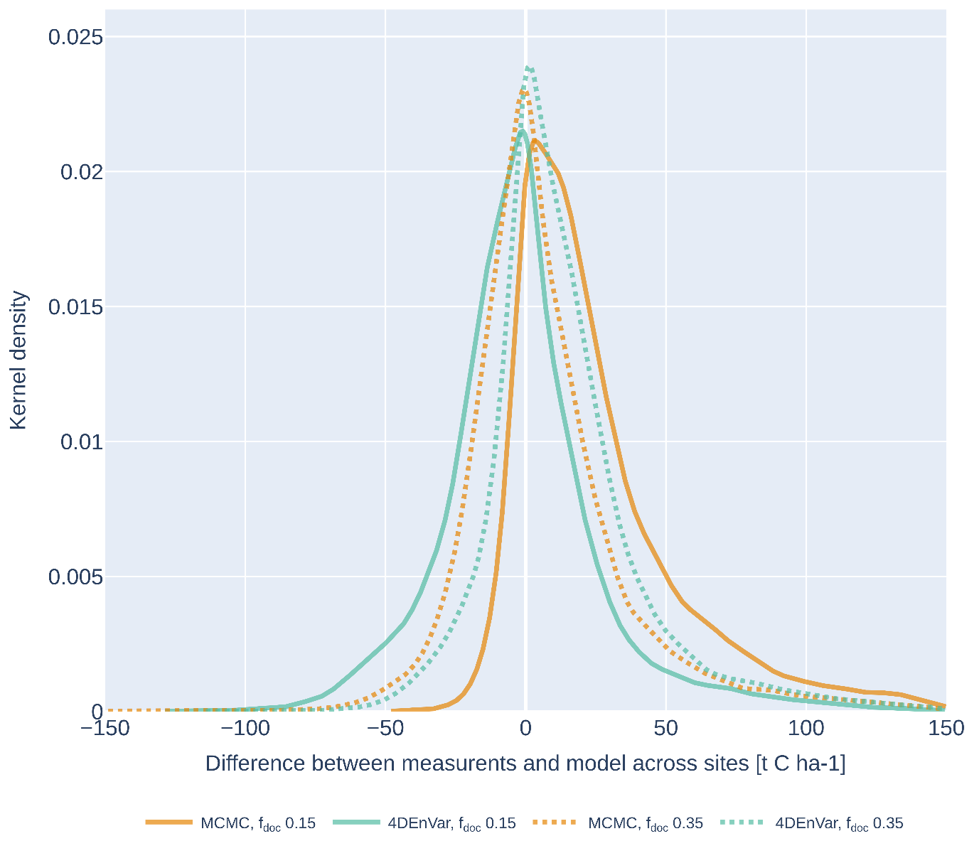
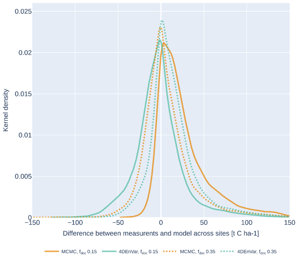
Figure 3 The validation dataset error distributions for both MCMC (orange) and 4DEnVar (green) calibrations with f_doc set to 0.15 (solid) and 0.35 (dashed).

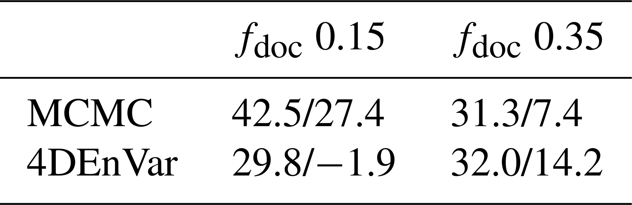
To examine the impact of the new parameter sets, Fig. 3 presents the differences between the measurements and model projections across all the validation sites, while Table 4 shows both the Root Mean Square Error (RMSE) and mean error (ME) representing bias in regard of the validation dataset for each parameter set. While the 4DEnVar parameter sets produces a somewhat symmetric error distribution around zero in both calibrations, with the higher f_doc there is a slight apparent tendency towards positive errors. In contrast, the MCMC error distribution shows a notable lean towards positive errors for the lower f_doc, while with the higher f_doc, the bias is much reduced. Since the SOC errors here are calculated as the measurement minus the model projection, this means that positive errors reflect the parameter set systematically underestimating the SOC projections. It is notable that with the higher f_doc, the RMSE values for the two parameterizations are very closer to each other even with the larger positive bias of the 4DEnVar method.

Table 4 The error statistics for the different parameterizations with regard to the validation dataset. The first value is for the root mean square error (RMSE) and the second for the mean error (ME). The unit for all the values is t C ha⁻¹.

To better comprehend what is causing the systematic MCMC error when f_doc, is lower, we further examined the actual calibration fit with both approaches in this scenario. Figure 4a shows how well the model SOC projections follow the measurements and in Fig. 4b the fit of the MAOM fraction with the 322 data points used for calibration. From these comparisons, it is evident that, while the 4DEnVar parameter set follows the measurement trend more closely than the MCMC, the latter calibration in turn replicates the MAOM : SOC fraction much better. We also note that there are also clear biases as the 4DEnVar parameters constantly underestimate the MAOM : SOC fraction, while there is a similar systemic underestimation of the total SOC with the MCMC parameters. When comparing the calibration fits for the higher f_doc (Fig. S3), the behaviour remains similar with calibration methods, although the differences between the measured and modelled values become smaller.

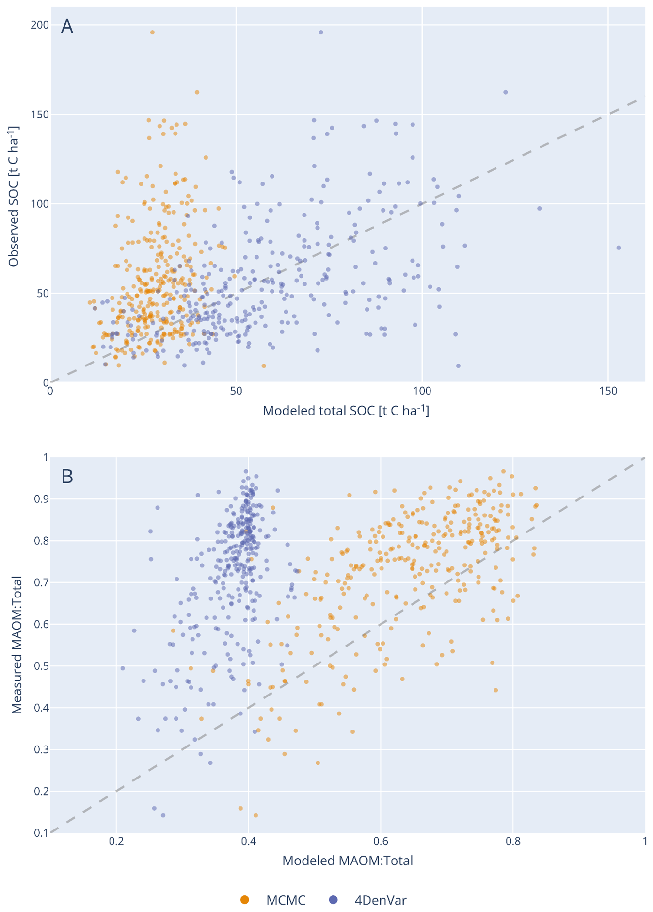
Figure 4 For the calibration dataset, comparison between the modelled and measured (A) Total SOC value and (B) MAOM : SOC fraction for both the MCMC and 4DEnVar calibrations when f_doc was set to 0.15.

When analysing of the cost function (J) for each estimated parameter set (Not shown), the MCMC calibration resulted in a lower J with the initial f_doc while, with the increased f_doc (i.e. from 0.15 to 0.35), the difference in J between the two approached was much reduced. However, when further looking at both total SOC and MAOM fractions measurements in both cases, the 4DEnVar produces a better match with total SOC while, conversely, the MCMC parameter set results in a closer fit with the MAOM fraction (MAOM : SOC) data. If we tighten the prior uncertainty used in the calibration, the 4DEnVar produces a different parameter set, though even those new parameters do still result in lower MAOM fractions in the validation dataset projections.

Figure 5 shows the spatial distribution of the errors in Europe for both the MCMC and 4DEnVar parameter sets. In the case of the lower f_doc, the MCMC underestimation is evident across Europe and, while the 4DEnVar map is more evenly distributed, there are also clearly more local overestimations than when f_doc is set higher. In the latter case, decrease in error can be seen across the whole Europe, with only a few clear areas, such as Nordic countries and the Iberian Peninsula, with consistent bias in the error. However, what is intriguing is that across central Europe, the prominent error points mirror each other. Where the MCMC parameter set produces overestimations, the 4DEnVar parameter set conversely results in underestimations.

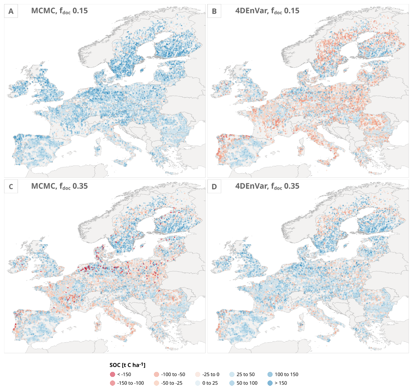
Figure 5 Spatial error distributions across the LUCAS validation sites for (A) MCMC with f_doc value of 0.15, (B) 4DEnVar with f_doc value of 0.15, (C) MCMC with f_doc value of 0.35, and (D) 4DEnVar with f_doc value of 0.35 parameter sets.

Because of the pronounced errors when f_doc is set to the lower value, we further examined the relationship of the SOC error with the NPP used as an approximation of the total litter input (Fig. 6). During this examination, it becomes evident that especially the MCMC parameter set projected a SOC underestimation clustered around low NPP values.

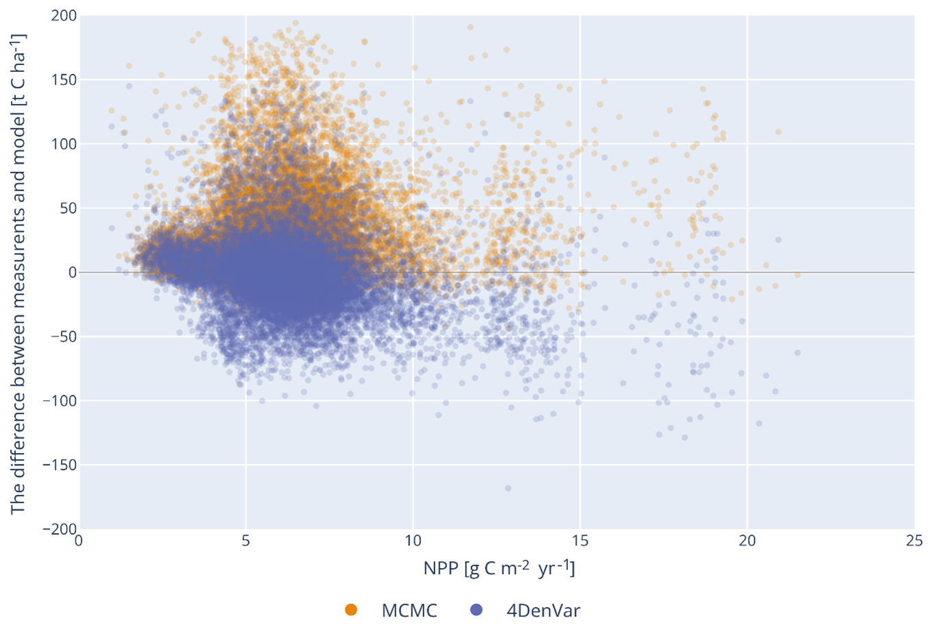
Figure 6 Relationship between NPP and SOC projection error for both calibrated parameter sets after f_doc was set to 0.15.

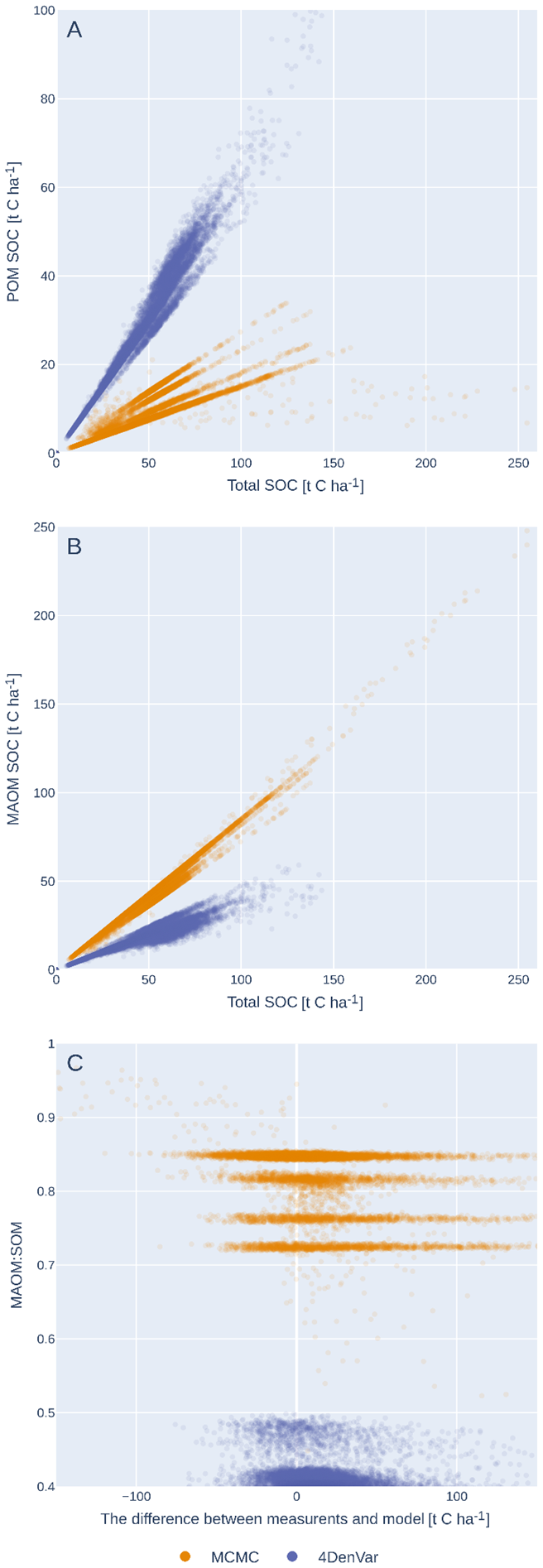
Figure 7 The model projected (A) POM, (B) MAOM stocks in relation to the total modelled SOC stocks as well as (C) The MAOM : SOM ratio in relation to the model error across the LUCAS sites after f_doc was increased from 0.15 to 0.35.

Finally, we examined the POM, MAOM and MAOM : SOC fractions in relation to the total projected SOC stock for the validation dataset with all calibrated parameter sets. Because of the systematic error when using the lower f_doc and, due to the general behaviour remaining similar between the two scenarios, we are only presenting the higher f_doc parameter set results here in Fig. 7 for clarity. With the POM (Fig. 7a) and MAOM (Fig. 7b), we can see similar differences between the two calibrations resulting from the initial calibrations. The MCMC parameterization still produces much higher MAOM stocks than 4DEnVar, and the latter parameterization contrastingly results in higher POM stocks. Additionally, POM with MCMC parameters remains at lower values than with the 4DEnVar parameters while, for the 4DEnVar parameters, MAOM hits a ceiling sooner than for the MCMC parameters. To further examine the impact of these behaviours on the projections, Fig. 7c illustrates the relationship between the MAOM fraction and model error across all the validation data points. Analysing the results further, we found that the very high SOC projections with both MCMC and baseline parameters occurred in specific circumstances, where both NPP and annual temperatures were low (not shown), and hence we attribute this to a structural issue within the model that arises in specific conditions rather than the parameterization per se.

4 Discussion

4.1 Comparison between the performances of MCMC and 4DEnVar calibration methods

As seen in the results, the 4DEnVar approach is a straightforward tool for calibrating the MEMS v1 model with LUCAS data, as valid as the MCMC approach. Both had issues with the first parameterization attempt when it came to the validation dataset, but performed similarly when the direct litter fraction to soil was increased. Hence, the central problem with the first calibration attempt was not due to the calibration method itself. This supports 4DEnVar as a meaningful approach for initial calibration of soil carbon models, especially considering the massive difference in the required computational costs. For MCMC, the 100 000 iterations used here took over a month to compute on our HPC server while, simulating the 250 ensemble members without using parallelization, took approximately four hours. It should be noted that the MCMC calibration did begin to converge to the final values already after 40 000 iterations, but there is a risk in accepting the local cost function minima after such a relatively short calibration cycle. The computational cost for calibration from having to spin-up to steady state is a known issue with land system models in general (Raoult et al., 2025).

What is striking, though, is how much the parameter sets produced by the two calibration methods in both litter distribution scenarios differ from each, even with the higher f_doc, they perform approximately equally well with regard to the total SOC measurements in the validation dataset. As mentioned in the Introduction, equifinality, a situation where there exists multiple parameter sets that produce similar model outputs, is a known issue in ecosystem modelling and is evidently represented by the results here. The notable element here is that the calibration method itself determines the resulting parameter set as even when repeated, the MCMC calibration approach does not suggest the solution is in the same part of the parameter space as the 4DEnVar results indicate. Generally, twin experiments are efficient first pass to test for equifinality and the challenge can be addressed by reducing the amount of parameters being calibrated, but here there are questions how much those efforts can be relied on in assessing equifinality.

While we are not certain of what is driving these systematic differences between calibration sets, we hypothesize that one crucial component is that the total SOC and MAOM fraction measurements appear to incentivize contradicting model behaviours. Our twin experiment results support this theory as, with synthetic datasets, we were able to retrieve the same parameter set of both total SOC and MAOM that internally coherent with the model dynamics. This tension is especially evident when the f_doc is lower and there is less litter to distribute between the SOC pools. In that situation, MCMC is still able to find a solution by forcing a reduction in the decomposition rate for the MAOM pool and increasing the decomposition rate for the POM pool. This leads to a high MAOM fraction but at the cost of lower POM pool values and, consequently, a tendency to project lower SOC values. Meanwhile, this conflict between the two measurement types does seem to cause issues with the gradient approach method applied by 4DEnVar to determine the ideal parameter set. This could be because the disagreement between the data sources will create such a degree of noise in the likelihood space that determining a correct gradient descent from a collection of ensembles will become much more challenging. Simultaneously, though, this vulnerability in the 4DEnVar could be exploited in future work to quickly test if different measurement types and drivers are compatible within the model framework.

These results further highlight the fundamental impact of the priors on the calibration results, especially with the 4DEnVar approach, that has been recognized as a larger challenge in ecosystem modelling (Dietze, 2017). While experimenting with the initial setup, we found that the 4dEnVar calibration produced unrealistic parameter values with negative decomposition rates, if prior was set to be too loose. This remained true even when increasing the f_doc value, although then the uncertainty could be loosened slightly more. Our hypothesis is that, while the MCMC iterative approach allows setting boundaries for the region where the values are sampled, such hard constraints are not present with the 4DEnVar. Additionally, the 4DEnVar does rely on the first order Taylor expansion, making it vulnerable to non-linear behaviours. Thus, incongruities resulting from missing model processes such as soil moisture, for example, can drive the parameterization beyond acceptable values if there is not a sufficient prior constrain implemented. This could be a partial explanation for the Iberian Peninsula error biases visible in Fig. 5 as the soil moisture dynamics are much more complicated in arid climates vulnerable to drought (Almendra-Martin et al., 2021). A further limitation is that the 4DEnVar algorithm used here draws the ensemble members by sampling the prior distribution. While this is a logical approach when those distributions are reliably approximated, here we do not know what the prior distributions are and must use a tight uncertainty range in order to avoid unrealistic estimations. Consequently, our application of 4DEnVar samples the parameter space in a more limited manner than would be preferable.

The lack of knowledge on prior distributions for the parameters is an obstacle that is further hindered by the lack of reliable measurement uncertainty estimates. An important aspect of Bayesian statistics is that the weight of an individual information source depends on how accurate it is in comparison to the other available information sources. Hence, the width of the prior uncertainty that we can assign to constrain the parameter estimate to remain in a reasonable range is dependent on the measurement uncertainty. In this work, those uncertainties were so low that we had to use a relatively narrow prior parameter range for the 4DEnVar approach. Furthermore, as detailed in the Methods section, we do not have reliable approximations of the measured MAOC : SOC fraction uncertainties. Their uncertainty here is, thus, defined by how much weight we wished to give them in relation to the total SOC measurements. When we tested a larger measurement error, which in turn allowed us to increase the prior parameter distribution for the 4DEnVar without producing unrealistic estimates, the 4DEnVar ensembles also changed with the new values moving farther away from the baseline values. The implication is that the 4DEnVar is much more sensitive to the measurement uncertainty representation than MCMC, due to how the prior constraint is applied.

Naturally this underlines the overall importance of providing reliable measurement uncertainties along with measurements themselves, but that is not something a model user can simply produce by themselves. When implementing the calibration, based on the results here we would recommend of initially looking through the calibration data and confirming that all the values there are sensible for the model/system being calibrated. As a more practical solution, it is possible to repeat the 4DEnVar calibration multiple times by using the previous posterior distributions as the priors to the next cycle. This way it is possible to ensure that the resulting parameter set is not simply because the prior had been set too far from the correct value and thus partially reduce the impact of the assigned prior distribution. However, the downside of repeating the calibration cycle in this manner is that not only does it reduce the impact of the prior, but each iteration reduces the resulting uncertainty distribution. Thus, the final parameter distributions would be artificially too confident. While the repeated calibration is a worthwhile tool in certain circumstances, it always needs to be implemented with great care and consideration.

4.2 The impact of the NPP assumption on the calibrated parameter set performance

Our results clearly underline how the fundamental assumptions regarding the NPP, as a litter proxy, impact the model calibration results. The lower f_doc resulted in a noticeable bias on total SOC predictions, especially with regard to the MCMC calibration. Another encouraging aspect of the work is that the differences between the two calibration methods results remain consistent even when changing the litter input assumption. This supports the capability of using the quicker 4DEnVar calibration to explore the impact of the NPP assumptions on the parameterization as any signal noted there should be reflected also in MCMC results.

What complicates future work is that coefficients associated with litter input are challenging to calibrate simultaneously with parameters associated with SOC decomposition, as their influence on the SOC overlap too much. It is important to note that while the focus in this experimentation has been the f_doc value, what it actually represents is the assumption of dividing NPP between upper- and below ground biomass as it reflects the amount of litter deposited directly into the soil. This is a central assumption that has to be included in some manner in SOC modelling and is represented by the plant species traits assigned to the surface vegetation. This highlights why better understanding of the vegetation qualities of the ecosystem being modelled is important for calibrating even simple SOC models.

As for even attempting to calibrate the NPP/litter coefficients simultaneously would first necessitate determining which exact coefficients would be calibrated. For example, in our case, there is first the question how well the MODIS NPP product represents reality for different systems. Then, part of that NPP is removed to represent economic activity before it is distributed to the four MEMS initial pools based on the three coefficients. Any of these three parts can be altered to change the final NPP input to the soil in different ways, but there is really no certainty at the moment what is the correct manner to better regulate the NPP based litter input. This complicated relationship in the surface vegetation driving litterfall and the SOC state has been shown in prior work such as in Raczka et al. (2021). There when they used remote sensing data to constrain their model state, while this improved their modelled aboveground biomass and carbon exchange accuracy, it also caused their modelled SOC accuracy to decrease because they were only using the aboveground data for both systems.

Adding to the challenges discussed above is that the various assumptions are not expected to be spatially homogeneous even in the same ecosystem type. For instance, the Nordic countries, especially Sweden and Finland, are dominated by economic forests where the NPP-to-litter pathway is heavily impacted by the growth stage as newly growing forest will have a large NPP, but not a corresponding amount of litter due to mortality. This could be connected to bias seen in the northern Europe in Fig. 5. Another example would be agricultural ecosystems as climate conditions affect which crops will be dominant in a given region. The type of crops naturally affects its traits as, for instance, the root depth distribution, which in turn is expected to impact the soil carbon stocks (Fan et al., 2016). These various components could be a reason why when analysing global soil databases, there is a weak statistical relationship between NPP and SOC despite that dynamic being well understood (Luo et al., 2021). Naturally this is not to questioning the use of NPP as a litter input for soil carbon models. Rather it is another reminder on how important it is to be aware of the various assumptions related to the NPP and remain consistent with them while running the calibrated model in various systems. Additionally, when doing future SOC projections, the uncertainties related to the various NPP/litter assumptions should be considered during analysis.

The error distributions for both calibration methods when applying the higher litter input is in itself worthy of analysis. The MEMSv1 model used is lacking several dynamics that are known to impact soil carbon stock, such as soil moisture (Falloon et al., 2011), various nutrient cycles (Gardenas et al., 2011; Feng et al., 2023) and mycorrhiza abundance (Hawkins et al., 2023). However, when considering the multitude of simplifications made to calculate the steady state approximations using parameters calibrated with data from 322 sites, the error distribution for the 17 000+ validation sites is much narrower than we initially expected. Which raises question how much of a further performance issue could be expected with addition of new processes? And, consequently, how can this limited data be used to evaluate which processes are most important for future projections?

Notably, while the spatial presentation of the model error under the higher f_doc shows only few regions where the differences between the two model errors are consistently larger than 10 t of carbon per hectare, such as the Nordic countries, the MAOM fraction projections by the two model calibrations differ systematically to a meaningful degree. For instance, 4DEnVar calibration resulted in a higher turnover rate of the MAOM pool, which in turn causes lower MAOM stocks. Both calibration methods are adjusting the parameters to produce lower total SOC, as the baseline parameters tend to overestimate the SOC stocks, but they solve the issue with very different representations of the internal SOC state that would have a major impact on future projections. With the current available information, it is not possible to evaluate which of the two states is more realistic; while the MCMC modelled MAOM fractions are on average high for all ecosystems (Georgiou et al., 2022), the LUCAS dataset leans towards arable soils where the MAOM fraction is expected to be larger in the top layer than for forests (Schrumpf et al., 2013; Sokol et al., 2022).

These outcomes emphasise the importance of carefully considering how model performance improvements are assessed with large-scale datasets such as the LUCAS measurement data, since the total SOC seems not sufficient which is in line with previous studies (Braakhekke et al., 2014; Guo et al., 2022). This is especially relevant as the model validation should be a crucial aspect of model choice regarding different SOC sequestration projects (Garsia et al., 2023). New measurement analysis methods allow for more efficient POM/MAOM fractioning of SOC samples (Leuthold et al., 2023), thus providing more detailed measurements to use during validation. However, as our results show, the SOC fractions might not be compatible with the total SOC measurements within the model context and indicate that there are missing processes within our model framework. Consequently, their value might be rather to evaluate what missing processes are needed within the model than validate existing parameterizations. Another approach for evaluation could be to examine the model performance within sub-regions or individual ecosystems instead of weighing it against the total dataset at once. A more nuanced approach to do this would be to use a hierarchical Bayesian approach (Gelman and Hill, 2007), but that requires more research on the applicability of that approach in solving the challenges highlighted by our results.

5 Conclusions

Calibrating soil organic carbon (SOC) models with large scale data sets is always a challenge due to the computational cost involved. Furthermore, numerous assumptions are made regarding model drivers that can potentially deeply affect the parameterization. In our work presented in this article, we have shown that 4DEnVar parameterization produces the approximately same RMSE for the validation dataset as the traditional and more cumbersome MCMC DEzs algorithm when the soil litter input is increased and actually outperforms in this metric the MCMC with the lower litter input. However, the parameter sets produced by the calibration methods differed from each other as did the model states they projected. Even though the total SOCs were similar, the difference between shorter lived POM and longer lived MAOM compounds was large enough to notably impact future projections. We also conducted a simple experiment to assess the impact of changing how the soil litter input is distributed among different litter pools. These results showed that while the litter input adjustment did impact the calibration, the general model behaviour produced by the two calibration methods remained similar. This implies, if it holds true with further testing, that the differences between the behaviours of the two calibration methods are not dependent on the driver data. Another facet of these results is that it confirms how large of an impact ecosystem related assumptions have on the resulting calibrations. The work here highlights how further consideration is required how to evaluate the model performances, especially on a larger scale. However, they also establish the fast 4DEnVar as a valid exploration tool that allows testing various scenarios with much more ease than the traditional MCMC approach. This will make it more pragmatically possible to assess how various assumptions impact ecosystem model results as well as better include those uncertainties in future projections as the various drivers are altered by climate change.