TRACE-Python: tracer-based rapid anthropogenic carbon estimation implemented in Python (version 1.0)

An implementation of Tracer-based Rapid Anthropogenic Carbon Estimation (TRACE), an algorithm for estimating anthropogenic carbon in the ocean, was produced using the Python coding language. TRACE is a transit time distribution approach intended to increase the accessibility of reliable and accurate anthropogenic carbon estimates. This algorithm produces estimates of ocean anthropogenic carbon as a function of user-supplied coordinates, time, seawater salinity, atmospheric carbon dioxide pathway, and optionally seawater temperature. We demonstrate the identical results of this implementation relative to its MATLAB predecessor, explore the sensitivity of anthropogenic carbon estimates to a newly-expanded range of available user input parameters, and suggest further lines of development for this software product as well as transient tracer-based ocean state estimation in general. Additionally, a new column integration routine was developed and deployed on anthropogenic carbon estimates generated from TRACE-Python when applied to the GLODAPv2.2016b gridded product temperature and salinity, yielding updated global and regional anthropogenic carbon inventories for the industrial era through the year 2500 along a range of atmospheric carbon dioxide trajectories. These inventories demonstrate satisfactory agreement with previous observation-based anthropogenic carbon inventories within the uncertainty of the estimate, demonstrating the skill of the TRACE method at the global level. This implementation of TRACE represents a step forward in accessibility to a wider user base, flexibility in user-specification of a greater number of estimation parameters, and skill as measured against other anthropogenic carbon estimates.

1 Introduction

Anthropogenic carbon in the ocean (C_anth) is defined as the increase in dissolved inorganic carbon (DIC) in seawater attributable to anthropogenic carbon dioxide (CO₂) emissions to the atmosphere over the industrial era. As the ocean is the largest single historical sink of CO₂ (Friedlingstein et al., 2023) and is expected to absorb most of the anthropogenic CO₂ transient on millennial scales (Archer et al., 1998), understanding the distribution and rates of change of C_anth in the global ocean is central to informing marine climate change effects and feedbacks (DeVries et al., 2023). On local scales, accumulation of C_anth gains further relevance as a driver of ocean acidification and other ecosystem disruptions that affect important natural resources (Doney et al., 2020). These disruptions underlie the need for accurate and accessible methods for estimating C_anth in the ocean.

Several methods for inferring C_anth from observational data have been devised. These can be separated into two classes: back-calculation and inversion. Back-calculation methods such as the ΔC^* (Gruber et al., 1996) and eMLR(C^*) (Clement and Gruber, 2018) techniques seek to estimate C_anth accumulation by isolating its effect on DIC from other biogeochemical processes. These techniques improved the understanding of the ocean carbon sink based on repeat hydrographic observations, but cannot extrapolate to unobserved periods, and the reliance on assumptions that complicate their interpretation including transient steady state invasion of anthropogenic signals, fixed nutrient and carbon stoichiometries, and simplified mixing models (Khatiwala et al., 2013; Müller et al., 2023). In contrast, inversion-based methods infer the propagation of a surface response to anthropogenic atmospheric CO₂ throughout the ocean via circulation constrained by measurements of chlorofluorocarbons (CFCs), sulfur hexafluoride (SF₆), and other tracers of ocean circulation (Hall et al., 2002; Haine et al., 2025), taking advantage of similarities between the atmospheric histories of these anthropogenic gases (Fig. 1). Inverted ocean tracer transport may be projected backwards and forwards in time, providing opportunities to explore changes in the ocean carbon sink (Khatiwala et al., 2009) and oxygen utilization (Sonnerup et al., 2015). Additionally, some inventory estimates have combined elements of both back-calculation and inversion methods (Sabine et al., 2004).

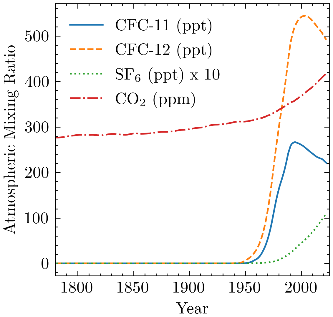
Figure 1 Atmospheric history of CO₂ and transient tracers CFC-11, CFC-12, SF₆ given as mixing ratios over 1780 to present. Transient tracers are given as global means of northern and southern hemisphere annual mean values from Bullister and Warner (2017). CO₂ is from the Mauna Loa time series (Keeling and Keeling, 2017) since 1958 and from the Law Dome reconstruction (Rubino et al., 2019) for earlier dates. Units are indicated in the legend as parts per million (ppm) or parts per trillion (ppt); note scaling of SF₆ by 10× to render it visible.

One subclass of inversion-based methods, the Transit Time Distribution (TTD), relies on a Green's function solution of the linear advection-diffusion transport equations to provide an age distribution representing the relative contributions of waters of various ages to a parcel, where age is considered to be the time since water was last at the ocean surface (Hall et al., 2002). This age distribution recognizes that interior ocean waters are more realistically represented as mixtures of many different water parcels of various ages carrying unique histories of atmospheric contact rather than by scalar ages (Waugh et al., 2003). The functional form of a TTD may vary, but an inverse-gaussian (IG) distribution specified as a function of transit time t (where smaller t indicates younger waters; Eq. 1) has been shown to describe tracer transport regimes of many ocean regions well in comparison with ocean general circulation models when the IG distribution is provided with optimal parameters (He et al., 2018). Its first temporal moment Γ (or mean age), and its second centered temporal moment Δ vary depending on interior location, but their ratio $\mathrm{\Delta }/\mathrm{\Gamma }$ is usually prescribed to be constant in solutions of Eq. (1), as described later.

$$\begin{array}{}\text{(1)}& \mathcal{G}\left(t\right)=\sqrt{{\displaystyle \frac{{\mathrm{\Gamma }}^{\mathrm{3}}}{\mathrm{4}\mathit{\pi }{\mathrm{\Delta }}^{\mathrm{2}}{t}^{\mathrm{3}}}}{e}^{\frac{-\mathrm{\Gamma }(t-\mathrm{\Gamma }{)}^{\mathrm{2}}}{\mathrm{2}t{\mathrm{\Delta }}^{\mathrm{2}}}}}\end{array}$$

This function describes one-dimensional pipe flow along isopycnal surfaces from a single source region, neglecting diapycnal diffusion and assuming steady-state circulation. Other formulations of the distribution representing more complex regimes require additional observational constraints (Holzer and Primeau, 2010). Convolution of the TTD 𝒢 with a surface boundary function propagates a surface signal (χ_s) through the ocean and allows calculation of its interior value (χ) as a function of time t at interior location r:

$$\begin{array}{}\text{(2)}& \mathit{\chi }(r,t)=\underset{\mathrm{0}}{\overset{\mathrm{\infty }}{\int }}{\mathit{\chi }}_{\mathrm{s}}(t-t^{\prime })\mathcal{G}(r,t^{\prime })\mathrm{d}{t}^{\prime }.\end{array}$$

Despite the utility of TTD methods for unraveling ocean tracer transport as well as recent calls for development of C_anth estimations based on transient tracers (Müller et al., 2023), their complex formulation and implementation has historically restricted their use. To overcome this barrier to more accessible science, an implementation of a TTD method was given by Carter et al. (2025) as “Tracer-based Rapid Anthropogenic Carbon Estimation version 1” (hereafter TRACEv1). Among the limitations of that implementation was its formulation using MATLAB (which while open-source is not freely available), and its dependence upon predetermined boundary conditions and TTD shape.

To address these limitations, this work describes an update of the TRACE routine and its implementation in the Python coding language. A brief overview of inherited methods is given followed by a description of new aspects of this implementation of TRACE, which encompass both practical improvements and fundamental changes to the method. This routine is validated against TRACEv1 to establish exact comparability, then used to produce an updated global gridded C_anth data product using an updated integration routine. A sensitivity analysis is then carried out to explore the effect of practical improvements to the TRACE method. Finally, we consider this method's strengths, limitations, and future development.

2 Summary of inherited methods

This implementation of TRACE in Python is both an exact replication of its MATLAB-based predecessor's results as well as an improvement in function. This work inherits the IG-TTD method implemented by its predecessor in form and function, and its equivalent results and the effect of improvements are described in Sect. 4. Hereafter, we use “TRACE” to refer to the algorithm, “TRACEv1” to refer to its implementation in MATLAB, and “TRACE-Python” to refer to its implementation in Python, for which this study used version 1.0.0. The main steps of this routine are enumerated with inputs bolded and outputs italicized for additional clarity, then described in detail:

1. User-provided location (latitude, longitude, depth), salinity, temperature, and optionally $\mathrm{\Delta }/\mathrm{\Gamma }$ predict the TTD and preformed properties via pre-trained neural networks. If temperature is not provided, it is first estimated by the remaining predictors.

2. The TTD is convolved with an atmospheric CO₂ surface boundary function chosen or given by the user to yield ocean pCO₂ at the user-specified time and location.

3. pCO₂ and pre-industrial pCO₂ are converted to DIC and pre-industrial DIC via inorganic carbon equilibrium calculation using preformed properties, salinity, temperature, and depth. Their difference yields C_anth, returned along with its uncertainty, mean age and intermediary parameters from previous steps in a CF-compliant dataset.

First, a pre-trained neural network predicts the TTD from latitude, longitude, depth, salinity, and temperature. The neural network training data consists of solutions to Eq. (1) optimized via the Nelder-Mead simplex optimization algorithm from paired CFC-11, CFC-12, and SF₆ observations in the GLODAPv2.2023 dataset (Lauvset et al., 2024) together with age estimates from the Ocean Circulation Inverse Model (DeVries, 2014). The cost function was the sum of squared normalized errors in partial pressures and age. The network architecture is composed of committees of neural networks like those used in Carter et al. (2021a). The shape of the IG-TTD (as specified by its first moment Γ and second moment Δ) was not originally allowed to vary from $\mathrm{\Delta }/\mathrm{\Gamma }=\mathrm{1.3}$; however, TRACE-Python makes $\mathrm{\Delta }/\mathrm{\Gamma }$ available as a changeable parameter, as described in Sect. 3.1. Adding this functionality required adding new neural networks for the age distributions fit to the same measurements with a set of ratios. The TRACE-Python now selects between the neural networks depending on the user provided ratio input. Similar neural networks predict preformed alkalinity, preformed phosphate, and preformed silicate (“preformed” indicating the properties that interior ocean seawater mixtures had when they at last contact with the ocean surface; Carter et al., 2021b). Failing to input a temperature predictor for any of these networks leads to temperature being predicted from salinity and location by an additional neural network.

Next, user specification of a global mean atmospheric CO₂ trajectory guides the formulation of a surface boundary condition. Built-in atmospheric CO₂ pathways include eight shared socioeconomic pathways (SSPs): 1-1.9, 1-2.6, 2-4.5, 3-7.0, 3-7.0-lowNTCF, 4-3.4, 4-6.0, and 5-3.4 (Meinshausen et al., 2020) and historical data with a linear extrapolation of the present increase (denoted Historical/Linear), all spanning the years 1–2500 CE. The user may also specify a custom pathway. TRACE estimates the surface boundary condition partial pressure of carbon dioxide (pCO${}_{\mathrm{2}}^{\mathrm{oce}}$) at a time t (in years) as a function of the time-varying atmospheric CO₂ mixing fraction XCO${}_{\mathrm{2}}^{\mathrm{atm}}\left(t\right)$:

$$\begin{array}{}\text{(3)}& \begin{array}{rl}p{{\mathrm{CO}}_{\mathrm{2}}}^{\mathrm{oce}}\left(t\right)& =X{{\mathrm{CO}}_{\mathrm{2}}}^{\mathrm{atm}}\left(t\right)-\mathrm{0.144}\times \left(X{{\mathrm{CO}}_{\mathrm{2}}}^{\mathrm{atm}}\left(t\right)\right.\\ & \left.-X{{\mathrm{CO}}_{\mathrm{2}}}^{\mathrm{atm}}(t-\mathrm{65}\mathrm{yr})\right).\end{array}\end{array}$$

This was derived as an empirical relationship between atmospheric and surface ocean trends in a model-observation hybrid product (Jiang et al., 2023), and it defines a surface boundary responsive to the rate of atmospheric increase or decrease over a 65-year lag time. Latitudinal variability in XCO${}_{\mathrm{2}}^{\mathrm{atm}}\left(t\right)$ is not considered in TRACE, as identifying a water mass source region and accompanying atmospheric boundary is beyond the application space of IG-TTD.

Finally, convoluting the surface boundary with the TTD (Eq. 2) yields ocean pCO₂ for a given location and time. This is converted to DIC via inorganic carbon equilibrium calculation with provided salinity, temperature, depth, and preformed properties as previously estimated. Subtracting pre-industrial DIC (calculated from a user-provided pre-industrial atmospheric mixing ratio and the same preformed properties) leaves C_anth. TRACEv1 assumed a pre-industrial XCO${}_{\mathrm{2}}^{\mathrm{atm}}$ of 280 ppm, which TRACE-Python makes more readily modifiable as an optional user input parameter, as described in Sect. 3.1.

This implementation of TRACE retains its predecessor's estimated uncertainty of C_anth point estimates and inventories. The estimated 1σ uncertainty of TRACE point estimates is the root sum of squared errors derived from a Monte Carlo analysis of error propagated from training data and error associated with a model reconstruction analysis. As with TRACEv1, the resulting uncertainty in C_anth likely underestimates the true reconstruction error in coastal, marginal, undersampled, and upwelling regions.

3 New capabilities

In addition to its inherited capabilities, TRACE-Python adds several features which expand its scientific applications and provide more robust results. We divide these into two categories: practical improvements (Sect. 3.1) that improve user experience and applications, and fundamental improvements (Sect. 3.2) that may alter the results or interpretation of the method.

3.1 Practical improvements

The practical function of TRACE is improved by an expanded array of optional user-accessible parameters to tune C_anth estimation. Now included in the main user-accessible function are options to adjust the shape of the IG-TTD distribution, to specify pre-industrial atmospheric XCO₂, to change inorganic carbon system equilibrium constants (i.e. PyCO2SYS input arguments Humphreys et al., 2022), and to provide or reuse preformed properties. These parameters facilitate adaptation of TRACE to changing scientific knowledge and needs, and create useful opportunities for comparison of the TRACE method with independent C_anth point estimates and inventories. Only the shape of the IG-TTD and the value of pre-industrial XCO₂ will be explored in detail here, as their impacts on C_anth estimates are expected to be the greatest. Lastly, TRACE-Python is made more transparent and repeatable with self-describing output. A call to its main function returns a Climate and Forecast (CF) compliant (Hassell et al., 2017) dataset recording all inputs and outputs, their units, and details of the computing environment. These data can be directly saved to the file system to facilitate data archiving and version control. This standardized self-documenting format is expected to enhance the interpretation and portability of TRACE-Python.

The shape of the IG distribution is specified by the ratio of its second and first moments: $\mathrm{\Delta }/\mathrm{\Gamma }$. The default value of the original and present implementations of TRACE is $\mathrm{\Delta }/\mathrm{\Gamma }=\mathrm{1.3}$, which has been found to minimize global mean error in ocean tracer simulations (He et al., 2018). Previous work has found values of $\mathrm{\Delta }/\mathrm{\Gamma }$ between approximately 0.1–5 in different regions (Sonnerup et al., 2015), while other studies have found over-constrained satisfactory IG solutions to occupy a more restricted range of 0.2–1.8 (Stöven et al., 2015; Raimondi et al., 2024). Spatial variability of $\mathrm{\Delta }/\mathrm{\Gamma }$ and the evolving scientific knowledge of ocean circulation is served by allowing TRACE users to vary $\mathrm{\Delta }/\mathrm{\Gamma }$, to which end a demonstration of its effect on estimated mean age and C_anth in a simulated transect and on the global C_anth inventory is given in Sect. 4.2. Internally, variability of $\mathrm{\Delta }/\mathrm{\Gamma }$ was enabled by retraining the neural networks estimating age distributions with IG shape characteristics constrained by discrete values $\mathrm{0.2}\le \mathrm{\Delta }/\mathrm{\Gamma }\le \mathrm{1.8}$ given in increments of 0.1, such that a user-provided $\mathrm{\Delta }/\mathrm{\Gamma }$ calls the age models of the nearest increment.

Pre-industrial atmospheric XCO₂ is typically defined between approximately 275 and 290 ppm, depending on the reference year defined as the beginning of the industrial era (Bronselaer et al., 2017). Differences in global C_anth inventories produced by TRACE under varying pre-industrial baseline atmospheric XCO₂ conditions are useful for reconciling estimates of C_anth inventories performed under varying reference years (cf. Müller et al., 2023) as well as global pre-industrial ocean XCO₂ distributions. This iteration of TRACE makes pre-industrial atmospheric XCO₂ accessible to the user in the main function, with a demonstration of the linear relationship between it and global C_anth inventories given in Sect. 4.2.

3.2 Fundamental improvements

The results and interpretation of the TRACE method are improved by two changes: First, a new method for routine integration of point estimates into column inventories was introduced. Second, a more rigorous and rapid inorganic equilibrium calculation was incorporated into the C_anth estimation. The first change is external to the C_anth estimation, while the second is a core element of estimation. Together, these improvements allowed for the production of a revised global C_anth inventory and reevaluation of the TRACE method alongside other C_anth estimation methods.

A new integration routine was implemented to facilitate rapid and repeatable estimation of column C_anth inventories. Some methods for numerical interpolation and integration of sparse profile data may produce unrealistic column properties and inventories from interpolation overshoots and discontinuities (Barker and McDougall, 2020), so the updated routine sought to avoid these qualities. A piecewise cubic hermite interpolating polynomial interpolation (Fritsch and Carlson, 1980) was performed between the most shallow and deepest C_anth estimate at each user-provided coordinate, followed by Romberg integration of the function produced by interpolation (Romberg, 1955). This routine aims to resolve high gradients of C_anth profiles among water masses while making minimal assumptions of data structure. The resulting column inventories are summed across regions of interest to yield regional or global C_anth inventories, as demonstrated in Sect. 4.1. During the development of TRACE-Python, a mistake related to layer thickness calculations was identified and corrected in the inventory calculation used by Carter et al. (2025) (the model reconstruction analysis and associated uncertainty estimate was unaffected). This led to the inventories that are presented herein being smaller on average than those presented previously, despite the nearly exact comparability between TRACEv1 and TRACE-Python results (Sect. 4). These new results should be considered more accurate reflections of the inventories implied by the TRACE approach and both sets of results remain generally strongly comparable with other literature estimates (Sect. 4.1).

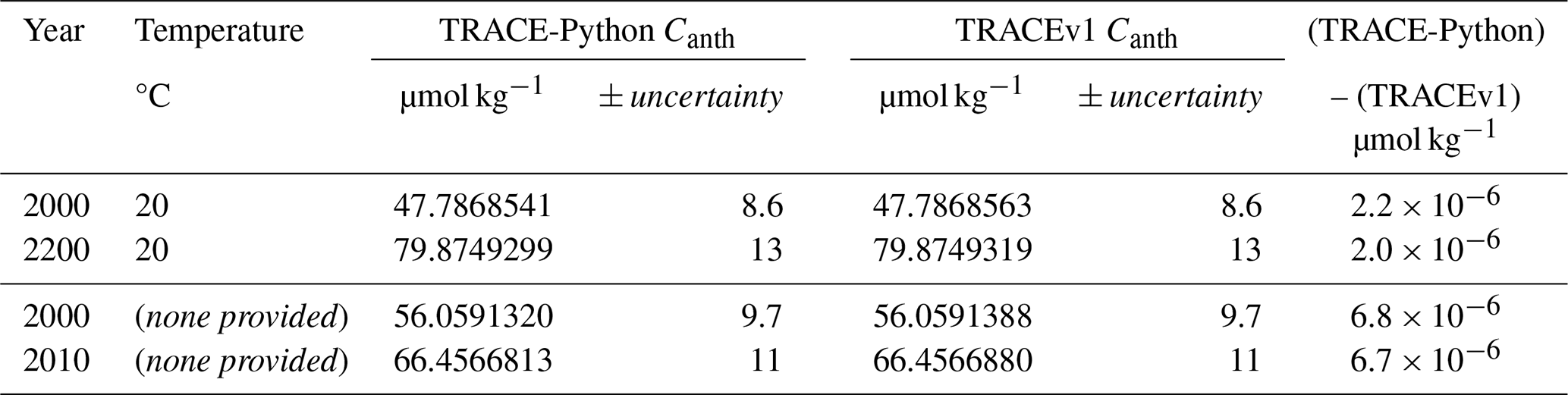
Table 1 Check values for C_anth given by TRACE-Python and TRACEv1 (the original MATLAB implementation) for four combinations of year, salinity, and/or temperature. All values were generated for the coordinates 0° N 0° E at 0 m depth with salinity set to 35 and the default $\mathrm{\Delta }/\mathrm{\Gamma }=\mathrm{1.3}$. The first two values assume SSP5-3.4, while the second two values assume Historical/Linear forcing. Missing temperature inputs as in the latter two check values were estimated from salinity and location using a neural network, which is not recommended for the most accurate behavior. The written precision of both TRACE-Python and TRACEv1 estimates was limited to the magnitude of their differences, rather than that of their accompanying uncertainties.

Inorganic carbon equilibrium calculation software was used for estimation of modern and pre-industrial DIC as a function of preformed properties and propagated CO₂ boundary conditions just as in TRACEv1, except for this updated TRACE method's use of PyCO2SYS (Humphreys et al., 2020), which did not require alteration of the solver function as was necessary for speed and performance in TRACEv1. Briefly, the solution of the inorganic carbon equilibria utilized by TRACEv1 via CO2SYS (version 1.1; van Heuven et al., 2011) was altered to increase the tolerance for pH error in the iterative numerical solver from $\mathrm{1}\times {\mathrm{10}}^{-\mathrm{4}}$ to $\mathrm{1}\times {\mathrm{10}}^{-\mathrm{3}}$ pH units, resulting in point C_anth estimates still within the estimated uncertainty of TRACE. The extent to which TRACE-Python estimates differ from TRACEv1 due to the former's use of a more rigorous inorganic carbon equilibrium solver is discussed in Sect. 4. TRACE-Python utilized PyCO2SYS version 2.0.0 without alteration, and produced point estimates of C_anth for all 1.1×10⁶ cells in the GLODAPv2.2016b gridded product for a single time step along the Historical/Linear CO₂ trajectory (see Sect. 4) in approximately 50 s (as the average of 10 runs) running on an Ubuntu 24.04.02 LTS machine with a 6-core Intel Core i5-9600K processor, versus approximately 60 s for the same estimation by TRACEv1 on the same hardware. We judge these times to be essentially comparable for most purposes.

4 Assessment

Assessment of TRACE-Python sought to validate its comparability with TRACEv1, explore its sensitivity to new user parameter inputs, and finally to demonstrate its use alongside other ocean C_anth data products. All estimates were produced with TRACEv1 (Carter, 2025b) and TRACE-Python version 1.0.0, which was developed and hosted in a Github repository (Sandborn and Carter, 2025) containing its source code, instructions for installation, documentation, demonstration scripts, and status badges indicating that the code passes internal consistency and validation tests. Comparability with TRACEv1 was established by calculation of check values as well as global gridded C_anth products using identical inputs. The two implementations were found to give identical results with precision approaching pmol kg⁻¹ levels, which when integrated into regional and global inventories led to no significant difference. Sensitivity analysis of newly-accessible parameters demonstrated increased flexibility of the TRACE-Python routine and pointed towards new directions for method development and software application.

Check values given for TRACEv1 and TRACE-Python (Table 1) demonstrated results within their respective uncertainties. Precision between MATLAB and Python implementations was expected to vary depending on the exact data types and operations performed: both languages include double-precision floating point arithmetic by default, but other contributors to point estimate imprecision can be expected on the order of 10⁻⁵ µmol kg⁻¹ from inorganic carbon equilibrium calculations alone (Humphreys et al., 2022).

A global gridded C_anth product was created using TRACE-Python, using seawater salinity, seawater temperature, coordinates, and depth from the GLODAPv2.2016b gridded product (Lauvset et al., 2016), which has a spatial resolution of 1°×1° and 33 depth horizons between the sea surface and 5500 m. Each of nine available atmospheric CO₂ pathways available in TRACE was employed to yield C_anth estimates for the years 1750, 1800, 1850, 1900, 1950, 1980, 1994.5, 2000, 2002.5, 2007.5, 2010, 2014.5, 2020, 2030, 2050, 2100, 2200, 2300, 2400, and 2500, chosen to align with previous literature global C_anth inventory estimates. These global C_anth gridded estimates are archived in a Zenodo repository (Sandborn et al., 2025a). Comparison of point C_anth estimates to the same analysis performed by TRACEv1 demonstrated agreement within uncertainties and approaching the limits of precision imposed by inorganic carbon equilibrium calculation. Their residuals (calculated as TRACEv1 estimates subtracted from TRACE-Python), across 9 atmospheric pathways, 20 timesteps, and 1.1×10⁶ ocean cells in the GLODAPv2.2016b gridded product, demonstrated a median error of $-\mathrm{1.8}\times {\mathrm{10}}^{-\mathrm{6}}$ µmol kg⁻¹ and median error of $-\mathrm{2.6}\times {\mathrm{10}}^{-\mathrm{6}}$ µmol kg⁻¹. While the total range of error was −0.02 to 0.0005 µmol kg⁻¹, 95 % of absolute error was less than $\mathrm{6.4}\times {\mathrm{10}}^{-\mathrm{3}}$ µmol kg⁻¹. TRACE-Python underestimation (relative to TRACEv1) of the global distribution of C_anth was most apparent for cells with higher C_anth (Fig. 2) which was repeatable for all CO₂ trajectories at all calculated times (Figs. A1–A6). This apparent bias is consistent with the magnitude of expected precision of (MATLAB) CO2SYS versus PyCO2SYS as previously noted. Extrapolating the median error given above across the entire ocean yields a value on the order of 10⁻⁵ Pg, so we conclude that random or systematic biases existing between implementations of TRACE had no significant effect on inventories calculated using this gridded product, as demonstrated in the calculation of regional and global C_anth inventories below.

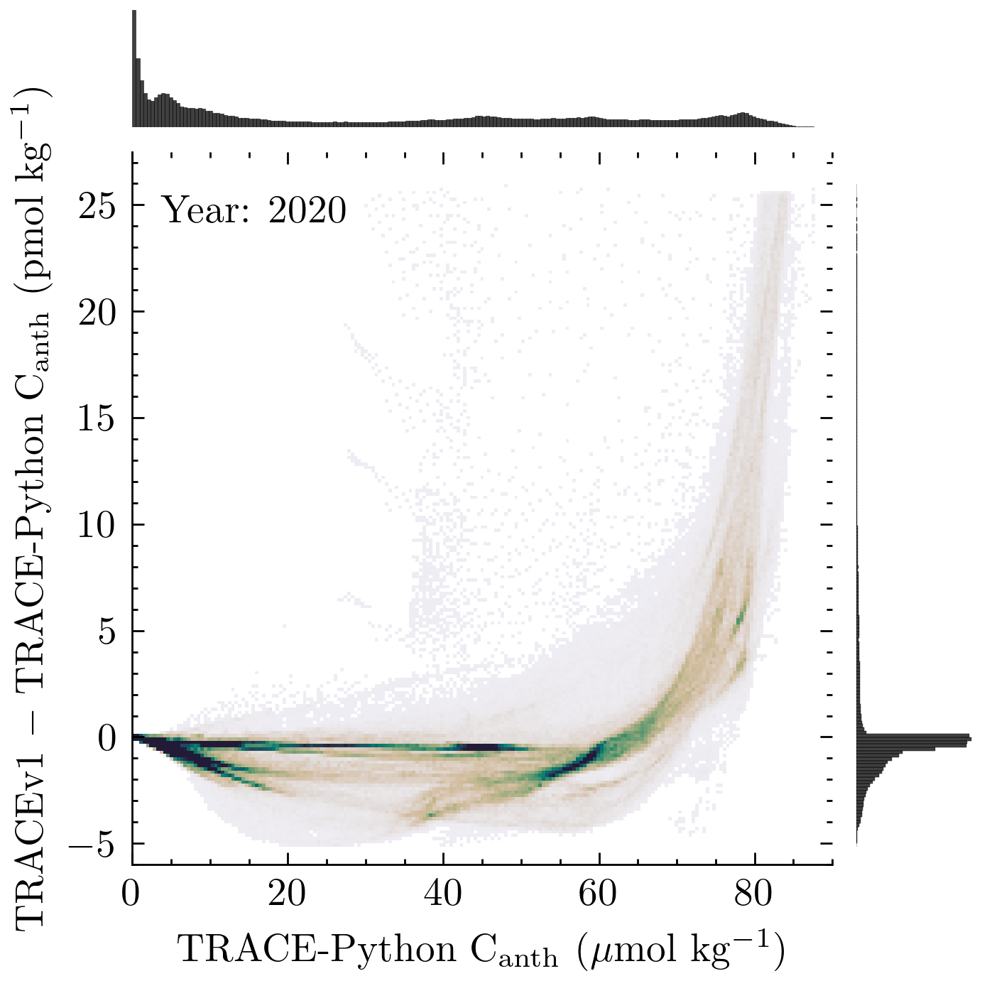
Figure 2 Histogram plot of 1.1×10⁶ residuals of TRACEv1 and TRACE-Python point estimates of C_anth against TRACE-Python point estimates of C_anth performed on the GLODAPv2.2016b gridded product for the year 2020. Shading indicates relative density of residuals within a histogram cell, with darker colors indicating higher density. The ordinate axis, given in pmol kg⁻¹, was limited to include 99 % of point estimates. The median residual for 2020 was $-\mathrm{4.7}\times {\mathrm{10}}^{-\mathrm{7}}$ µmol kg⁻¹, and the total range was $\mathrm{2.5}\times {\mathrm{10}}^{-\mathrm{4}}$–$-\mathrm{5.7}\times {\mathrm{10}}^{-\mathrm{6}}$ µmol kg⁻¹. The majority (>83 %) of residuals were within pmol kg⁻¹ range.

4.1 Global and regional inventories

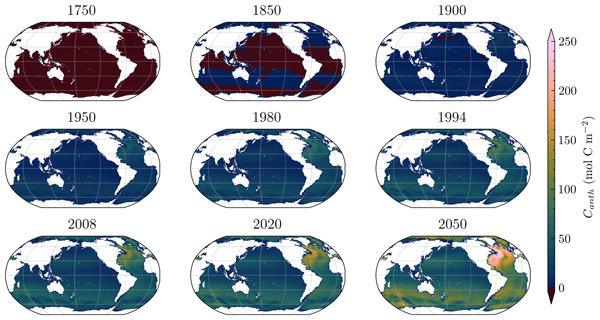
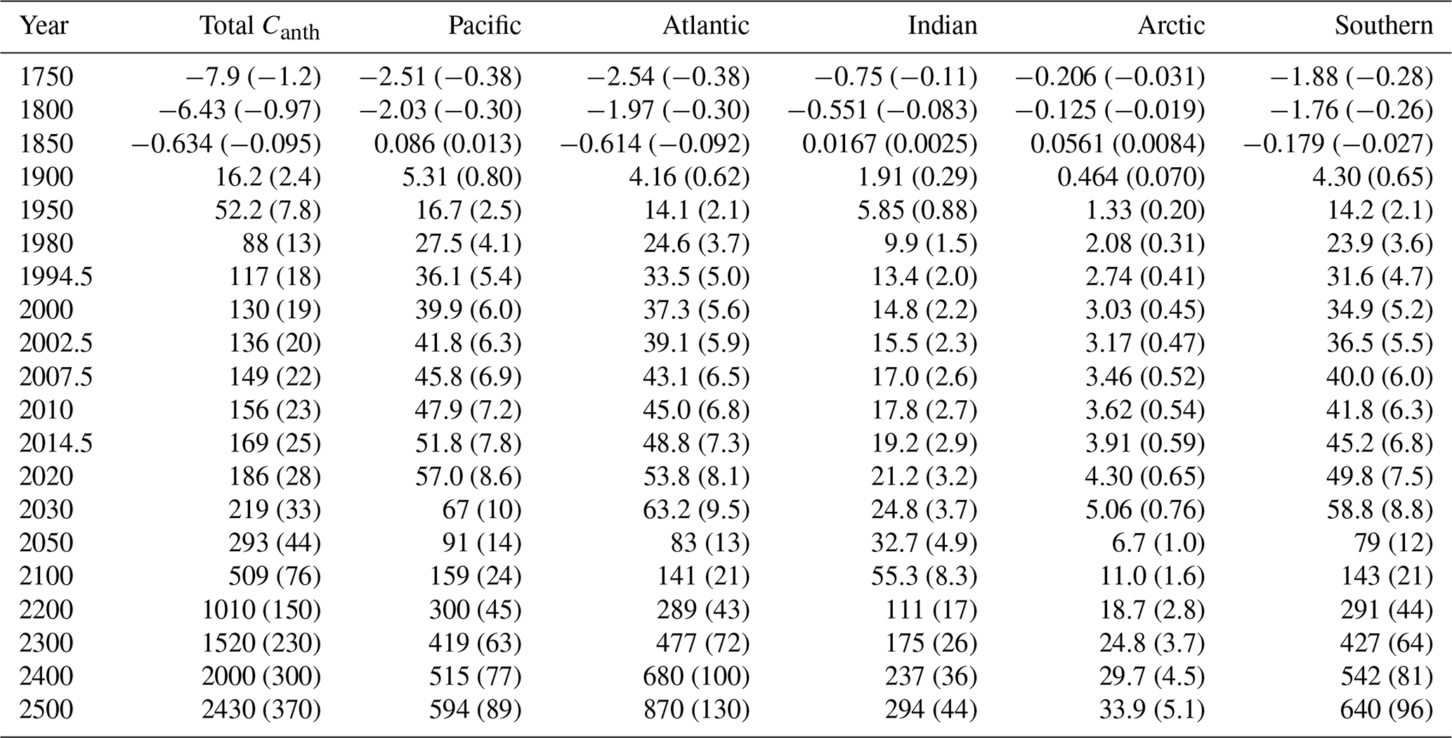
Column inventories for the global C_anth gridded product were calculated using the integration method described in Section 3.2. Each 1°×1° cell of the sea surface grid was assigned a surface area as in Fay et al. (2021) and summed to give regional and global C_anth inventories using basin definitions after Fay and McKinley (2014) (Table 2). These inventories varied from those given in Carter et al. (2025) as a result of this work's improved integration method, yet yielded a similar illustration of uneven storage of C_anth in the global ocean (Fig. 3) in qualitative agreement with previous C_anth inventories. Applying the updated integration to the TRACEv1 gridded product gave statistically-indistinguishable regional and global C_anth inventories (Table C1), which were smaller than those of Carter et al. (2025) by approximately 7 % for the period 1990–2015. We believe that an erroneous cell volume calculation was employed in the latter product which was not noticed until after the independent formulation of the updated inventories in this work.

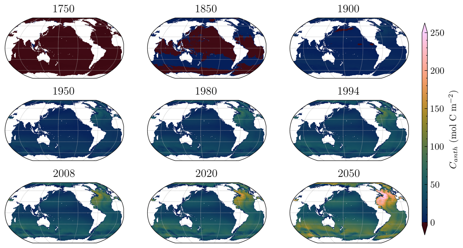
Figure 3 Column inventory of C_anth mapped for indicated years produced via TRACE analysis of the GLODAPv2.2016b gridded product assuming historical atmospheric CO₂ trajectory. Major C_anth sinks associated with deep water formation in the North Atlantic and Southern Oceans are visible in the propagation of elevated C_anth waters from these regions. Regions with negative column C_anth inventories were observed in the Pacific ocean until approximately 1900 due the imposition of a pre-industrial XCO₂ definition of 280 ppm on old, deep waters formed under conditions of marginally lower xCO₂.

Table 2 Estimate of global and regional ocean C_anth inventories produced via TRACE-Python analysis of the GLODAPv2.2016b gridded product. Basins are defined after Fay and McKinley (2014). Values are given as Pg C ± 1σ uncertainty as for TRACEv1.

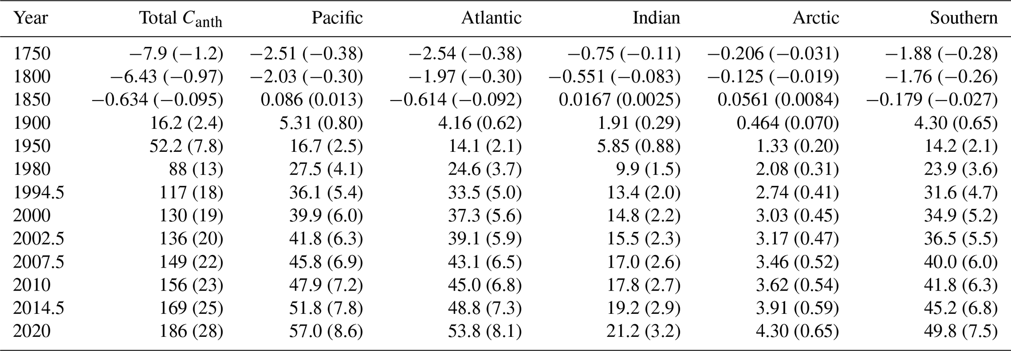
Similarly, this integration was applied to the C_anth estimates in the GLODAPv2.2016b gridded product (Lauvset et al., 2024) for ease of comparison, yielding a global C_anth inventory of 164±29 Pg C for the year 2002, which compares favorably with the inventory of 167±29 Pg C given by Lauvset et al. (2020). In all cases, the improved inventory estimation approach yielded smaller inventory estimates which happen to be more closely aligned with previous literature estimates. However, the decreases in the inventories were small relative to uncertainties and the updated TRACE global C_anth inventory with other previous data-based estimates (Fig. 4) did not qualitatively alter the conclusions of Carter et al. (2025).

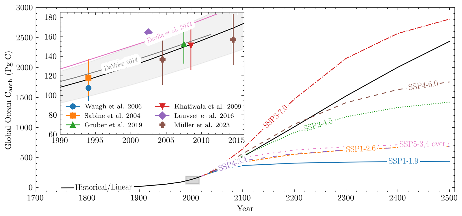
Figure 4 Global ocean C_anth inventories assuming indicated atmospheric CO₂ pathways produced via TRACE analysis of the GLODAPv2.2016b gridded product. Global ocean C_anth inventory estimates from the literature are shown with their uncertainties alongside the TRACE estimate in an inset figure, in which the uncertainty of the TRACE estimate is shown as a grey band. The estimate of Khatiwala et al. (2009) is shown with an 11 Pg C increase to account for exclusion of the Arctic ocean as suggested in that work. The estimate of Waugh et al. (2006) is decreased by 20 % to account for varying air-sea disequilibrium as suggested in that work. The estimate of Lauvset et al. (2016) published as the GLODAPv2.2016b gridded product was integrated using the same method as TRACE-Python, as described in Sect. 4.1.

Agreement with DIC-based approaches (Sabine et al., 2004; Müller et al., 2023; Gruber et al., 2019) was good, while agreement with TTD- and inversion-based approaches (Davila et al., 2022; Lauvset et al., 2016; DeVries, 2014; Khatiwala et al., 2009; Waugh et al., 2006) remained more variable. In particular, the IG-TTD inventory estimate of Lauvset et al. (2016) continued to be the most serious outlier, potentially due their differing treatment of atmospheric CO₂ disequilibrium, lack of SF₆ age constraint, and potentially other factors (cf. Sect. S9 Carter et al., 2025). The rate of C_anth accumulation over 1990–present was nearly identical in TRACE-Python global C_anth inventory compared to Davila et al. (2022), yet greater than given by DeVries (2014) despite the additional constraining role of the latter inversion in TRACE. Differences in the magnitude and rate of C_anth inventory change between the inversions of DeVries (2014) and Davila et al. (2022) are thought to be the result of regional differences in circulation field strength constrained by different sets of tracers, and the same is likely true for TRACE; however, further investigation of representations of C_anth accumulation is beyond the scope of this work.

Projected global ocean C_anth inventories in Fig. 4 (see also Table B1) indicated a range of potential outcomes of selected SSPs. The continued increase of each pathway's C_anth inventory through the year 2500 indicated continuing C_anth uptake by the ocean due to ventilation of presently-deep waters regardless of mitigation trajectory. Similarly, mapped column inventories for future dates (Fig. 3) demonstrated the increasingly unequal spatial distribution of ocean C_anth in the 21st century. In this way, TRACE provides a robust and accessible tool for exploring how mitigation efforts may be expressed in the past, present, and future ocean.

4.2 User input sensitivity

Among the practical improvements accomplished in this work (Sect. 3.1) was the addition of a wider array of parameters for C_anth estimation made accessible to the user. While this allowed for more flexibility in application, it necessitated improved understanding of the relationship between these parameters and TRACE C_anth estimates. To this end, we assessed the effects of altering two user-accessible parameters within reasonable bounds. This process illustrated sensitivity associated with parameter selection, explored the robustness of the method, and pointed to avenues of investigation which will improve the IG-TTD method and its comparability with other C_anth estimation methods.

The effect of shifting the pre-industrial atmospheric CO₂ mixing fraction is to change the time at which ocean C_anth began accruing, and thus to alter C_anth inventories at all times before and after that point. To demonstrate this effect, C_anth global inventories were generated assuming historical atmospheric forcing as in Sect. 4.1, varying pre-industrial atmospheric XCO₂ between 270 and 290 ppm (Fig. 5a). The resulting set of inventories demonstrated a linear relationship with pre-industrial atmospheric XCO₂ for any year, with a slope of approximately −10 Pg C ppm⁻¹. This suggested a straightforward empirical mechanism for comparing inventories performed on the basis of different pre-industrial XCO₂; however, adjusting estimates performed on the basis of a pre-industrial cutoff year introduces the additional step of converting the year to an atmospheric CO₂ fraction consistent with the atmospheric forcing of the method, which may not always be in evidence. As an example, the global ocean C_anth estimate of Khatiwala et al. (2009) was performed on the basis of a pre-industrial cutoff year 1765, at which point the global annual mean atmospheric XCO₂ in this work was approximately 278 ppm. Adjusting this to a basis of 280 ppm would involve a simple 20 Pg C decrease, which would worsen agreement but maintain overlap in their respective uncertainties. This simple corrective mechanism is most suitable for qualitative demonstration, as it remains unclear how C_anth inventories in other works would shift were they carried out with higher or lower pre-industrial atmospheric XCO₂ basis. Furthermore, some approaches do not integrate C_anth over regions of the ocean with low signal-to-uncertainty ratios, and the magnitude of this correction would decrease with the volume of the ocean considered. For these reasons, the observation-based C_anth inventory estimates in Fig. 4 remain unadjusted for pre-industrial atmospheric CO₂. Model-based inventory estimates also provide opportunities for application of the TRACE-derived pre-industrial atmospheric CO₂ sensitivity in aiding analysis of C_anth inventory model-observation mismatch.

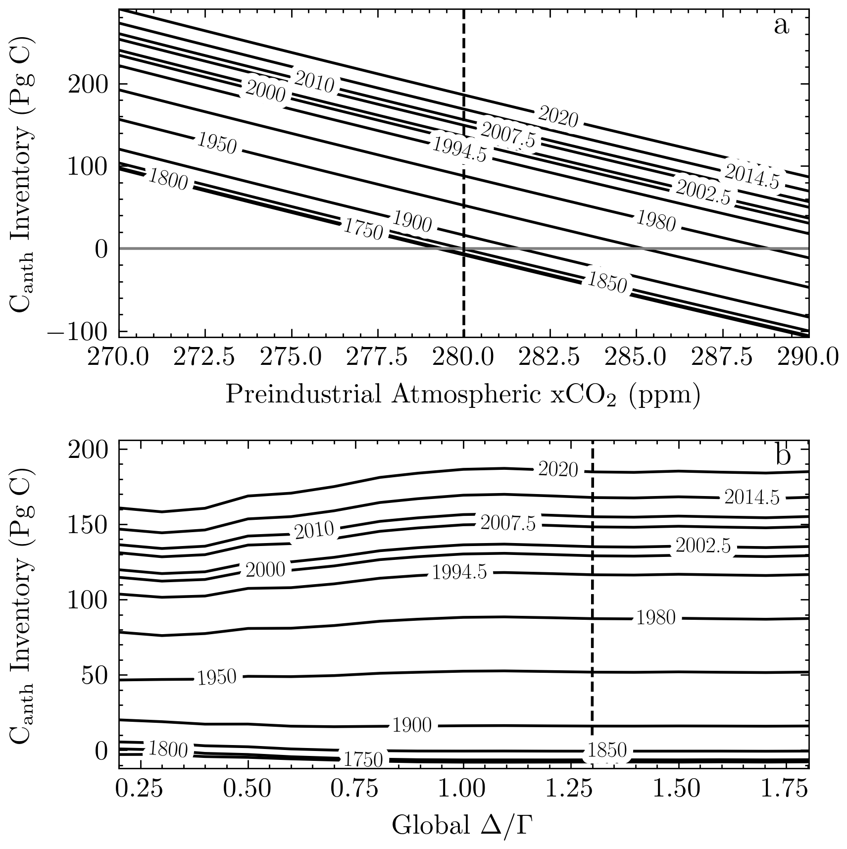
Figure 5 TRACE-estimated global ocean C_anth inventories at indicated years assuming: (a) varying pre-industrial atmospheric CO₂ concentrations or (b) varying IG-TTD $\mathrm{\Delta }/\mathrm{\Gamma }$. A linear relationship was expressed between pre-industrial atmospheric CO₂ and all years' inventories. The relationship between $\mathrm{\Delta }/\mathrm{\Gamma }$ and ocean carbon C_anth inventories displayed asymptotic behavior, with sensitivity decreasing at high $\mathrm{\Delta }/\mathrm{\Gamma }$. Vertical lines in both figures represent the TRACE defaults.

Underestimation of Global Ocean Biogeochemical Model (GOBM) inventories relative to observation-based products could be explained to the extent that GOBM C_anth inventories grow by adjusting them to earlier starting dates. A GOBM ensemble prepared for the REgional Carbon Cycle Assessment and Processes phase 2 (RECCAP2) project (DeVries et al., 2023) gave a mean 1994 global inventory of 83±15 Pg C and a 2002 mean of 102±12 Pg C, or 29 % and 25 % smaller than TRACE estimates (Table 2). This systematic underestimation of the ocean carbon sink by GOBMs likely arises from biases in carbon biogeochemistry and variable dates for the beginning of the industrial era, which for the RECCAP2 models ranged from 1765–1870 CE. (Terhaar et al., 2024). They found that delaying a model's start date from 1765 to 1850 led to an decrease between 18.2–22.7 Pg C (in agreement with the sign of the correction suggested in the TRACE sensitivity analysis), and suggest that this range could be too low by 40 %. The RECCAP2 GOBM ensemble's c. 34 Pg C underestimation relative to TRACE at the beginning of the 21st century could then be partly explained by this effect, but without knowledge of the starting dates of ensemble components, their assumed atmospheric XCO₂ histories, and whether a similar linear sensitivity is observed for those models, further analysis must be left to future work. This sensitivity analysis supports the idea that global ocean C_anth inventory model-observation mismatch can be explained at least in part by the definition of the baseline, or pre-industrial, atmospheric XCO₂.

Shifting the baseline atmospheric XCO₂ (or year) of C_anth accumulation also changed the pre-industrial baseline of ocean XCO₂, which in volume-weighted distributions of TRACE estimates broadened and increased from a narrow range of 276.95±0.03 ppm (mean ± SD) in 1750 CE to 280±1 ppm in 1850 CE (Sect. D). These values (and those of intermediate years) represent effective global ocean circulation-informed pre-industrial XCO₂ distributions for common starting points of ocean state estimates. These sensitivity analyses demonstrated the utility of TRACE to inform and compare C_anth inventories and pre-industrial inorganic carbon distributions in future work.

The shape of the IG-TTD age distribution is modified by changing $\mathrm{\Delta }/\mathrm{\Gamma }$, which by default is equal to 1.3. Increasing $\mathrm{\Delta }/\mathrm{\Gamma }$ increases the ratio of isopycnal diffusion to advection in the one-dimensional pipe flow framework of the IG solution (Waugh et al., 2003). The sensitivity of this parameter in TRACE was tested by varying $\mathrm{\Delta }/\mathrm{\Gamma }$ in increments of 0.1 between 0.2 and 1.8 in order to reconstruct C_anth global inventories assuming historical atmospheric forcing as in Sect. 4.1. The resulting global C_anth inventories increased with $\mathrm{\Delta }/\mathrm{\Gamma }$ up to 1.0, above which varying $\mathrm{\Delta }/\mathrm{\Gamma }$ had little effect on inventories (Fig. 5b). This contrasts with the findings of He et al. (2018), which found IG-TTD C_anth inventories for 2002 decreased by approximately 80 Pg C over the range $\mathrm{0.2}\le \mathrm{\Delta }/\mathrm{\Gamma }\le \mathrm{1.8}$. This contrast can be explained by the fact that TRACE integrates mean ages from the Ocean Circulation Inverse Model in its IG-TTD optimization, perhaps stabilizing the optimization especially in older, deeper waters with relatively little transient tracer content. This contrast should receive further study in the interest of improving interpretations of inversion-based methods of C_anth estimation.

Regional variability of $\mathrm{\Delta }/\mathrm{\Gamma }$ poses a further problem which can be addressed with TRACE-Python. In order to illustrate the regional effects of varying $\mathrm{\Delta }/\mathrm{\Gamma }$, mean age and C_anth were estimated by TRACE along the WOCE A16 transect using salinity, temperature, and coordinates from its 2013–2014 occupation by the CLIVAR program (CCHDO Hydrographic Data Office, 2023). $\mathrm{\Delta }/\mathrm{\Gamma }$ values of 0.4, 0.8, and 1.2 were chosen to span a domain of rapid C_anth change illustrated by Fig. 5a, and the resulting hydrographic profiles (Fig. 6) illustrated the expected inverse relationship of C_anth and mean age. Lower values of $\mathrm{\Delta }/\mathrm{\Gamma }$ were associated with higher vertical gradients as relatively “young” waters were confined to the surface. Note that a single average value o  $\mathrm{\Delta }/\mathrm{\Gamma }$ was imposed for all water masses in this example. The previously-noted spatial variability of $\mathrm{\Delta }/\mathrm{\Gamma }$ was not implemented, and is left to further research. Detailed hydrographic description and discussion of water masses and consequences of regional concentration of C_anth is beyond the scope of this work; instead, this sensitivity experiment demonstrates the potential for TRACE to test the effect of variable $\mathrm{\Delta }/\mathrm{\Gamma }$ on ocean mean age and C_anth. This demonstration also does not consider suitability of the IG-TTD framework to constrain age distribution for water masses with complex mixing regimes (cf. Stöven et al., 2015).

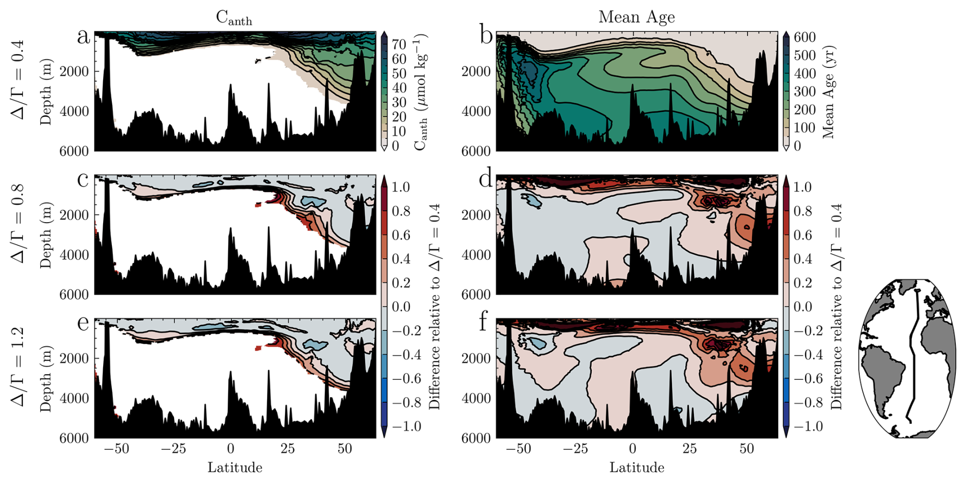
Figure 6 TRACE-estimated C_anth concentration (a, c, e) and mean age (b, d, f) along the WOCE A16 transect (inset map) for the year 2013, calculated using three values of $\mathrm{\Delta }/\mathrm{\Gamma }$ spanning the range of greatest change in C_anth inventory. C_anth estimates with magnitudes smaller than their estimated uncertainties are not plotted in (a), and these same values are neglected in (c, e). The second two rows are plotted relative to the values of the first row for ease of comparison. Lower values of $\mathrm{\Delta }/\mathrm{\Gamma }$ are associated with less anthropogenic CO₂ invasion and younger thermocline waters at all latitudes.

We conclude that varying $\mathrm{\Delta }/\mathrm{\Gamma }$ above approximately 1.0 will not lead to major changes in water mass age or C_anth as estimated by TRACE, but smaller values of $\mathrm{\Delta }/\mathrm{\Gamma }$ lead to notable changes in mean age and C_anth distribution and inventory. Similarly, increasing pre-industrial XCO₂ decreased C_anth inventories, suggesting a method for comparing the results of this routine with other products. The parameter tuning of the TRACE routine demonstrated here by varying pre-industrial XCO₂ and $\mathrm{\Delta }/\mathrm{\Gamma }$ emphasized its flexibility, which recommends it for further investigation of these parameters of the IG-TTD method.

5 Discussion

This work described an implementation of the TRACE method for the estimation of ocean C_anth in Python, incorporating several practical and fundamental improvements. The effect of these changes is to increase the accessibility and breadth of application of this tool, while providing a firmer scientific footing with clearer understanding of input parameter sensitivity. This updated version demonstrated equivalent function to the original product when given identical input, ensuring comparability across research products and users. The development of the TRACE method and its software implementations gains further currency when considered as part of a broader dialogue between scientific questions and research tools to address them. This work in particular has benefited from co-development with Empirical Seawater Property Estimation Routines (ESPER), which similarly use location, salinity, temperature, and other predictors to estimate DIC, total alkalinity, pH, nitrate, phosphate, silicate, and oxygen concentrations (Carter et al., 2021a; Dias and Carter, 2025). This family of seawater property estimation methods is of value to scientific, marine management, and earth observing communities, who use these estimation routines to compare against observations, fill in unobserved regions, initialize models, and make informed management decisions.

The practical and fundamental improvements to TRACE described and demonstrated in Sect. 3 provided an opportunity to test the sensitivity of TRACE to pre-industrial XCO₂ and the shape of the TTD within the constraints of the IG framework. Global C_anth inventories were sensitive to both parameters within the range of values given by previous work. The spatial distribution of mean age and C_anth were similarly altered by $\mathrm{\Delta }/\mathrm{\Gamma }$ along a reconstructed meridional transect of the Atlantic Ocean. Given the variability in inferred $\mathrm{\Delta }/\mathrm{\Gamma }$ associated with different water masses (cf. Sonnerup et al., 2015), future work using TRACE could investigate the interaction of regionally-varying $\mathrm{\Delta }/\mathrm{\Gamma }$ on water mass age and C_anth. This sensitivity analysis of ocean C_anth and mean age to parameters of the TRACE method illustrates the importance of careful investigation of the assumptions of ocean state estimate routines. While TRACE-Python retains reasonable default values of these and other input parameters in common with TRACEv1, they are made accessible and tunable with the intention of aiding future investigation and expanding the applicability of this software tool.

Several other parameters and assumptions central to the TRACE method are not user-tunable, and consideration of these suggests room for continued method validation and improvement. In particular, its surface CO₂ disequilibrium does not vary in space, it prescribes transient tracer atmospheric saturation, C_anth is assumed to equal the entire change in DIC since the pre-industrial era, it estimates preformed alkalinity and nutrients and assumes their invariance in time, and the IG-TTD implies steady state one dimensional pipe flow transport of transient signals into the ocean interior along isopycnals. A model-based review of uncertainties of the IG-TTD method found that transient tracer and C_anth saturations were the greatest contributors to uncertainty (He et al., 2018), so continued development of TRACE and other TTD-based ocean state estimation routines can be served by targeted investigation of the transient tracer and C_anth surface boundary conditions and their variability in time and space. Unfortunately, transient tracer saturations cannot yet be modified in TRACE without retraining its neural networks. These shortcomings represent a continuing opportunity for comparing TRACE output with models and ocean observations.

We emphasize that TRACE, ESPER, and their seawater property estimation peers cannot replace observation; rather, they rely on continued monitoring providing the physical and chemical basis for accurate estimation. Ocean hydrography becomes increasingly-important in the face of climate change as Earth experiences extremes moving it outside its previously-observed state captured by property estimation routines. In light of the changing and improving picture of the ocean system to be gained from future observations, TRACE will continue iteratively improving its estimation of C_anth. Future GLODAP releases will better constrain TTDs with the addition of more and better tracer constraints and preformed property estimates, while the advance of global ocean circulation and biogeochemical models may indicate more accurate parameterized relationships between the atmospheric anthropogenic CO₂ increase and its ocean sink.

6 Outlook

The development of TRACE has occurred in parallel to and in some cases dependent on related ocean chemistry software. This includes other property estimation routines (Carter et al., 2021a, b; Dias and Carter, 2025; Carter et al., 2017), inorganic carbon equilibrium and air-sea flux calculations (Humphreys et al., 2022; Sharp et al., 2020; Orr et al., 2015; Gregor and Humphreys, 2021; Lewis and Wallace, 1998) and seawater thermodynamic toolboxes (Firing et al., 2021). Further development of this suite of open-source software tools should seek to incorporate new findings and techniques, maintain dependency and interoperability, and respond to the needs of users in order to pursue high-quality and accessible ocean chemistry data practices.

It is anticipated that TRACE will continue to be developed without fundamentally altering its core approach, while continuing to reliably offer results with well-documented assumptions and consistency across implementations. Potential directions for further development include integrating future GLODAP releases in its training data, exploring the impact of other reanalysis products on estimates, including updated atmospheric CO₂ trajectories, and refining TTD shape and surface transient tracer and C_anth disequilibrium assumptions. As methods for estimating C_anth continue use and development, a more comprehensive understanding of their differences, assumptions, and uncertainties should be formed. This need gains currency in light of the present need to understand the effects of climate change mitigation and marine carbon dioxide removal on the ocean carbon cycle. Future work in pursuit of these needs should seek to advance the practice of C_anth estimation from scientific and applied perspectives.

Appendix A: Gridded product comparison

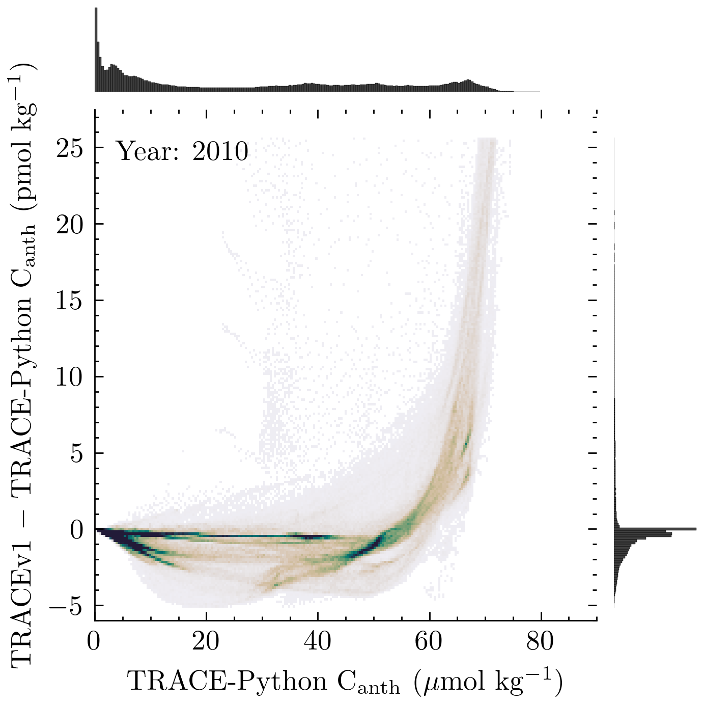
The distribution of the differences, or residuals, of the TRACEv1 and TRACE-Python gridded data products indicated close agreement for results in 2020 (Fig. 2). The same analysis produced for other years illustrates that this agreement holds for other periods as well (Figs. A1–A6).

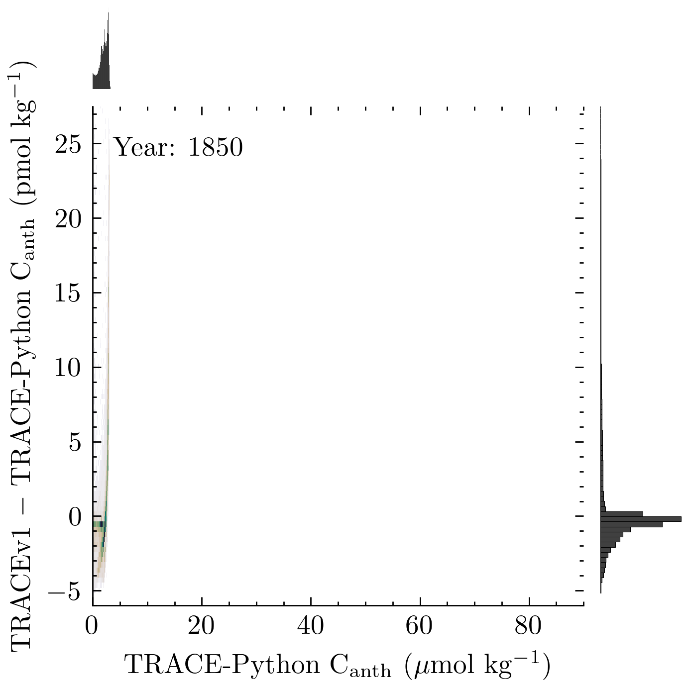
Figure A1 Histogram plot of the residuals of TRACEv1 and TRACE-Python point estimates of C_anth against TRACE-Python point estimates of C_anth performed on the GLODAPv2.2016b gridded product for the year 1850 given the historical CO₂ trajectory. The ordinate axis, in units of pmol kg⁻¹, was limited to include 99 % of point estimates.

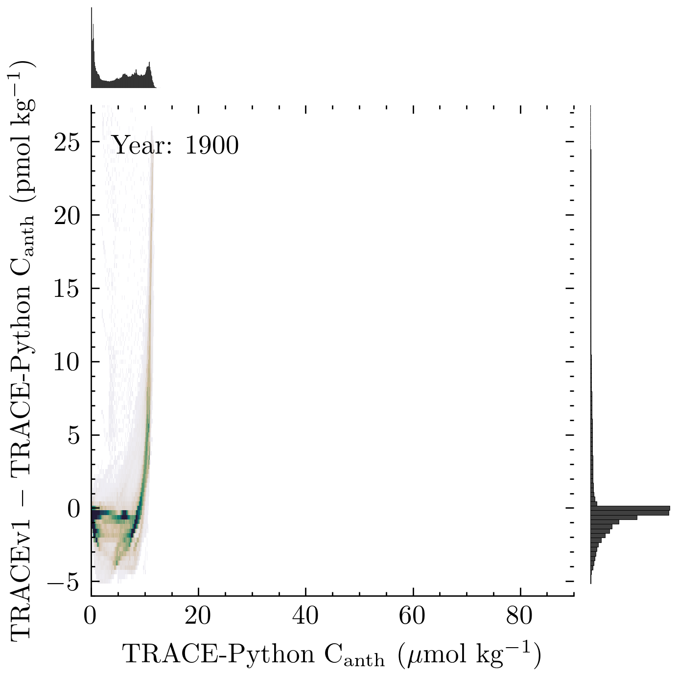
Figure A2 Histogram plot of the residuals of TRACEv1 and TRACE-Python point estimates of C_anth against TRACE-Python point estimates of C_anth performed on the GLODAPv2.2016b gridded product for the year 1900 given the historical CO₂ trajectory. The ordinate axis was scaled as in Fig. 2.

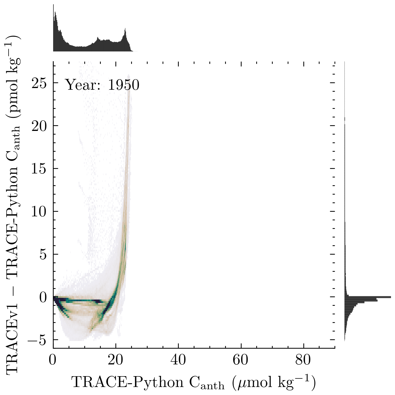
Figure A3 Histogram plot of the residuals of TRACEv1 and TRACE-Python point estimates of C_anth against TRACE-Python point estimates of C_anth performed on the GLODAPv2.2016b gridded product for the year 1950 given the historical CO₂ trajectory. The ordinate axis was scaled as in Fig. 2.

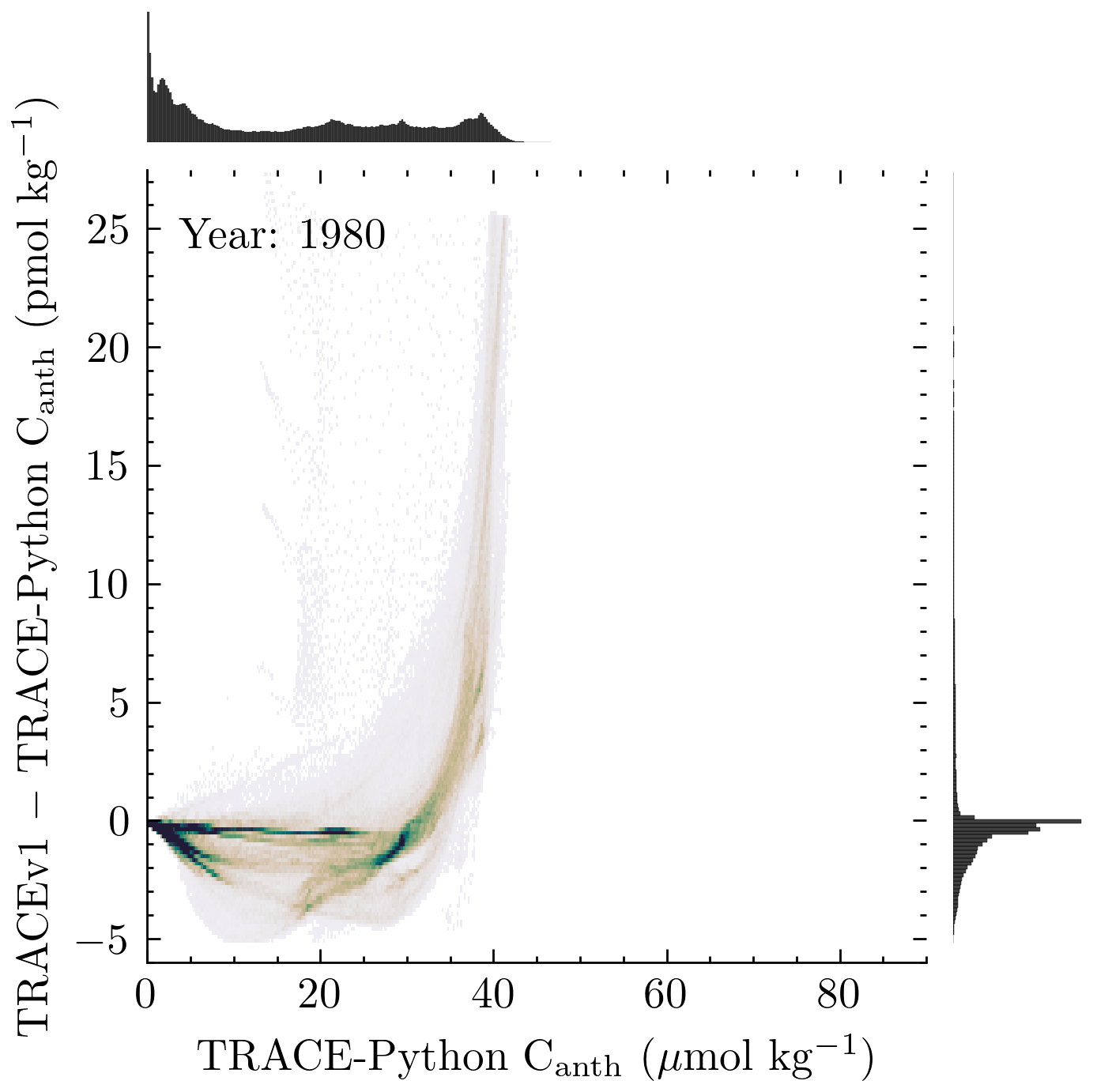
Figure A4 Histogram plot of the residuals of TRACEv1 and TRACE-Python point estimates of C_anth against TRACE-Python point estimates of C_anth performed on the GLODAPv2.2016b gridded product for the year 1980 given the historical CO₂ trajectory. The ordinate axis was scaled as in Fig. 2.

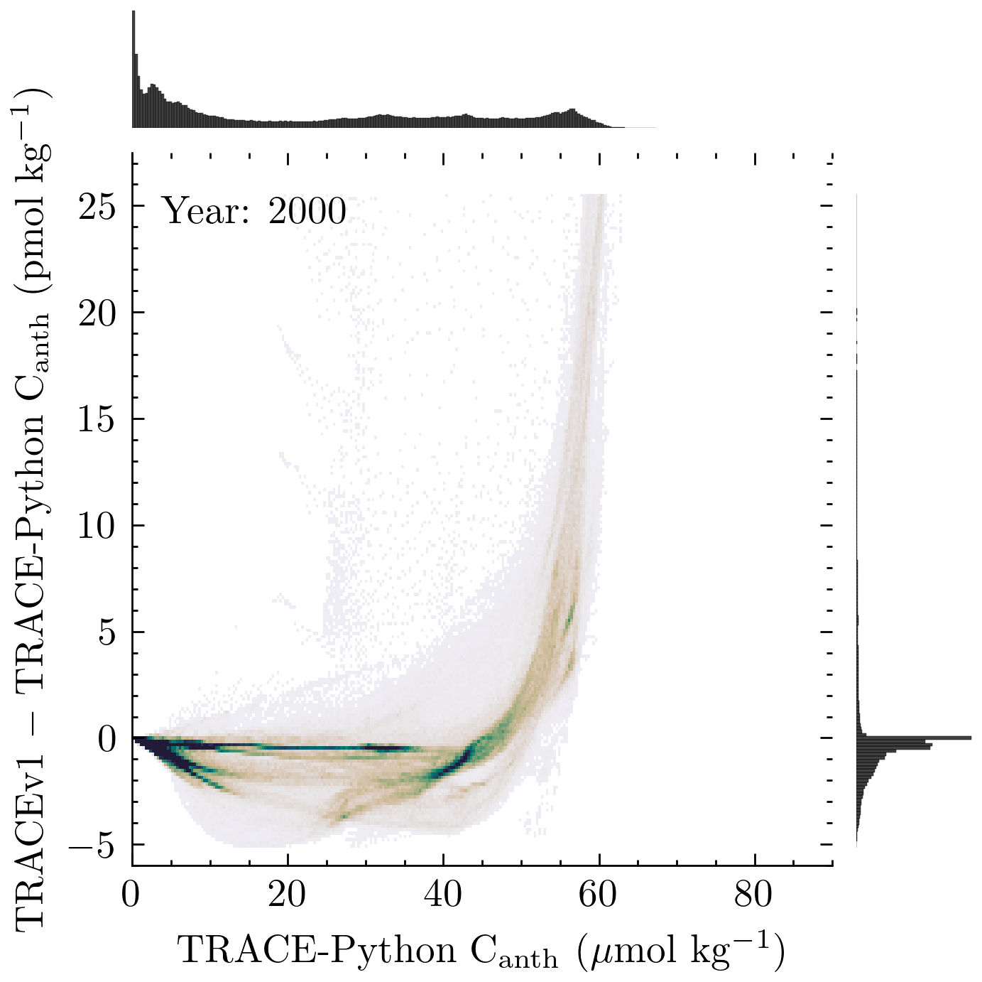
Figure A5 Histogram plot of the residuals of TRACEv1 and TRACE-Python point estimates of C_anth against TRACE-Python point estimates of C_anth performed on the GLODAPv2.2016b gridded product for the year 2000 given the historical CO₂ trajectory. The ordinate axis was scaled as in Fig. 2.

Figure A6 Histogram plot of the residuals of TRACEv1 and TRACE-Python point estimates of C_anth against TRACE-Python point estimates of C_anth performed on the GLODAPv2.2016b gridded product for the year 2010 given the historical CO₂ trajectory. The ordinate axis was scaled as in Fig. 2.

Appendix B: Projected C_anth inventories

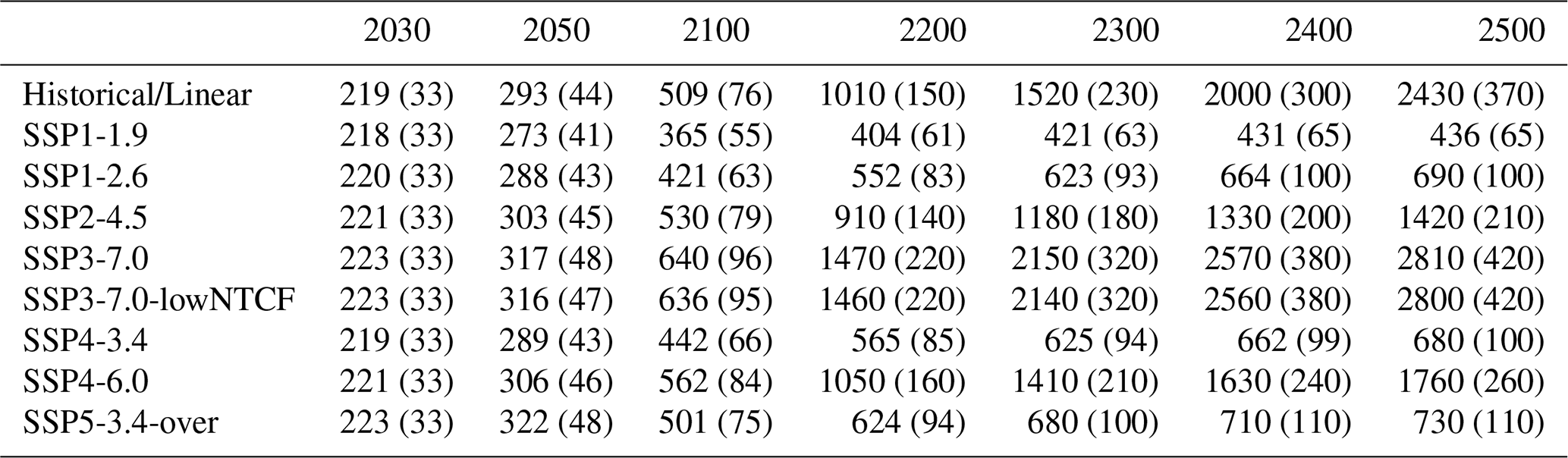
Among the strengths of TTD-based C_anth inventories is the ability to project forward and backward in time under certain assumptions (Sect. 1). The inventories illustrated by Fig. 4 after the year 2020 are given in Table B1 with uncertainties.

Table B1 Projections of global ocean C_anth inventories produced via TRACE analysis of the GLODAPv2.2016b gridded product under varying atmospheric CO₂ trajectories. Values are given as Pg C ± 1σ uncertainty.

Appendix C: Updated TRACEv1 C_anth inventories

Application of the updated column and areal integration method described in this work (Sect. 3.2) to the original TRACEv1 gridded C_anth product (Carter, 2025a) yielded identical results to that produced in this work (Table 2), demonstrating their functional equivalence (Table C1).

Table C1 Estimate of global and regional ocean C_anth inventories produced via TRACEv1 analysis of the GLODAPv2.2016b gridded product and integration using the updated method. Basins are defined after Fay and McKinley (2014). Values are given as Pg C ± 1σ uncertainty.

Appendix D: Pre-industrial Ocean XCO₂ distributions

Volume weighted distributions of ocean XCO₂ were produced from the gridded data product described in this work (Sandborn et al., 2025a) by performing a kernel density estimation analysis weighted by the volume of each cell in the product, along with summary statistics as reported in the main text (Sect. 3.2 and in the accompanying plot (Fig. D1). Three years spanning the range of commonly-reported “pre-industrial” dates were considered, along with 2020 CE for comparison of the distributions. The same distributions and statistics may be readily obtained from the published dataset for any year listed in the tables of this work, or for an intervening year by performing a TRACE analysis of the GLODAPv2.2016b or another suitable gridded product.

The extremely narrow distribution of ocean XCO₂ in Fig. D1a resulted from the imposition of a CO₂ boundary condition given by Eq. (3) on the pre-industrial stable atmospheric curve. Broadening and general increase of the distributions visible in Fig. D1b–d represents the propagation of that boundary condition through the global ocean, resulting in the present-day bimodal XCO₂ distribution representing highly-ventilated waters with XCO₂ approaching the atmospheric condition alongside poorly-ventilated waters maintaining XCO₂ little-removed from the pre-industrial state.

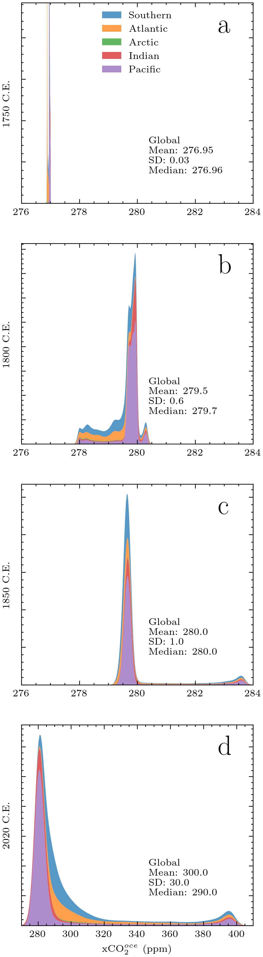
Figure D1 Volume-weighted kernel density estimates of ocean XCO₂ (XCO${}_{\mathrm{2}}^{\mathrm{oce}}$) and summary statistics estimated for the global ocean by TRACE from the GLODAPv2.2016 gridded product temperature, salinity, and coordinates, colored and stacked by ocean basin defined as in the main text. (a–c) XCO₂ distributions for the years 1750, 1800, 1850 CE, illustrating the variability of ocean XCO₂ within the range of years previously given as “pre-industrial” starting points for ocean observational or modeling state estimation. (d) XCO₂ distribution for the year 2020 CE provided for comparison. Note the horizontal coordinate is identical for (a)–(c) to aid comparison of distribution shifts, but extended for (d) to capture the broadened distribution.