ClimateBenchPress (v1.0): a benchmark for lossy compression of climate data

The rapidly growing volume of weather and climate data, both from models and observations, is increasing the pressure on data centers, restricting scientific analysis, and data distribution. For example, kilometre-scale climate models can generate petabytes of data per simulated month, making it generally infeasible to store all output. To address this challenge, numerous novel compression techniques have been proposed to ease data storage requirements. However, there exist no well-defined benchmarks for rigorously evaluating and comparing the performance of these compressors, including their impact on the data's properties. The lack of benchmarks makes it difficult to design and standardize compressors for weather and climate data, and for scientists to trust that compression errors have no significant impact on their analysis. Here, we address this gap by presenting ClimateBenchPress, a benchmark suite for lossy compression of climate data, which defines both data sets and evaluation techniques. The benchmark covers climate variables following various statistical distributions at medium to very high resolution in time and space, from both numerical models and satellite observations. To ensure a fair comparison between different compressors, each variable comes with a set of maximum error bound checks that the lossy compressors need to pass. By evaluating an initial set of baseline compressors on the benchmark, we gather practical insights for effective application of lossy compression. Our benchmark is open source and extensible: users can easily add new compressors, data sources, and evaluation metrics depending on their own specific use cases.

1 Introduction

Datasets quantifying Earth's weather and climate are rapidly growing in size due to the advent of next-generation km-scale Earth system models (ESMs) (Stevens et al., 2019; Bauer et al., 2021; Rackow et al., 2025; Segura et al., 2025) and an expanding suite of satellite missions monitoring the Earth's atmospheric state (Rossow and Schiffer, 1991; Schmit et al., 2017; Stephens et al., 2002; Illingworth et al., 2015). These datasets can easily reach petabyte scale (Bauer et al., 2021), requiring very large data centers with significant energy consumption and slowing down data analysis and sharing. Hence, there is an urgent need for novel compression algorithms that can handle the unique characteristics of climate data.

Lossless compressors cannot provide sufficiently large compression ratios due to the high entropy in the mantissa of the floating-point representation of the data (Klöwer et al., 2021), limiting compressibility following Shannon's source coding theorem (Shannon, 1948). However, climate data comes with inherent uncertainty associated with each data point owing to measurement, model, and simulation errors that vary in space, time, and for different variables. Additionally, the precision required from the input data varies widely depending on the downstream analysis a user might want to conduct. As an example, computing the expected average global mean temperature rise from ensembles of ESM simulations is robust to uncorrelated spatial errors that will cancel upon averaging. Therefore, a lower level of precision is required than computing the expected power generation of wind farms from high-resolution storm-resolving models which requires precise knowledge of wind speeds at specific locations. In climate data there is generally a tolerable compression error, though defining exact, or at least practical, error tolerances for all data and downstream analyses remains an open problem.

The existence of a tolerable compression error motivates the usage of lossy compression algorithms. As the name implies, in contrast to lossless compression, lossy compression no longer guarantees that the original input and the reconstructed output after decompression are identical. However, by allowing for a non-zero reconstruction error, lossy compression is generally able to achieve significantly larger compression ratios compared to lossless compression (Baker et al., 2016; Underwood et al., 2022). There exists already a wide body of work on developing lossy compressors tailored to scientific datasets (Ballester-Ripoll et al., 2019; Underwood et al., 2022; Liang et al., 2022; Lindstrom, 2014; Silver and Zender, 2017; Zhao et al., 2020) and an emerging field are neural compression schemes for climate data (Huang and Hoefler, 2023; Han et al., 2024; Mirowski et al., 2024)¹.

However, at the time of writing, no well-established and easily accessible benchmark exists that is focused specifically on the task of compressing climate and weather data. The issue is complicated by the fact that compression algorithm developers tend not to be experts in climate science, and although abundant data exist, much of it is either difficult to access or stored in formats unfamiliar to researchers outside of climate science. This leads a majority of research to focus on evaluating compressors on datasets derived from a single model or data source, as can be seen in Fig. 1. Without questioning the importance of any single dataset, it is important to validate compressors across a variety of data sources to test their general application. Each dataset, from varying models or observations, poses different challenges for compression due to differing resolution in space and time, statistical distributions of variables, variable characteristics, associated uncertainty, and scientific objectives. For example, temperature fields are generally smooth with strong correlations in both space and time, precipitation fields often have large gradients, contain a large number of zeros and have a long tail of extreme values, whereas sea surface temperature fields are only defined over ocean regions and therefore contain large number of missing values. The differences between individual variables can be so stark that they might require different compression approaches altogether (Baker et al., 2017). However, a sufficiently general compressor should be able to deal with the diversity of variable characteristics found in climate datasets. It is important that a compression benchmark adequately captures this diversity.

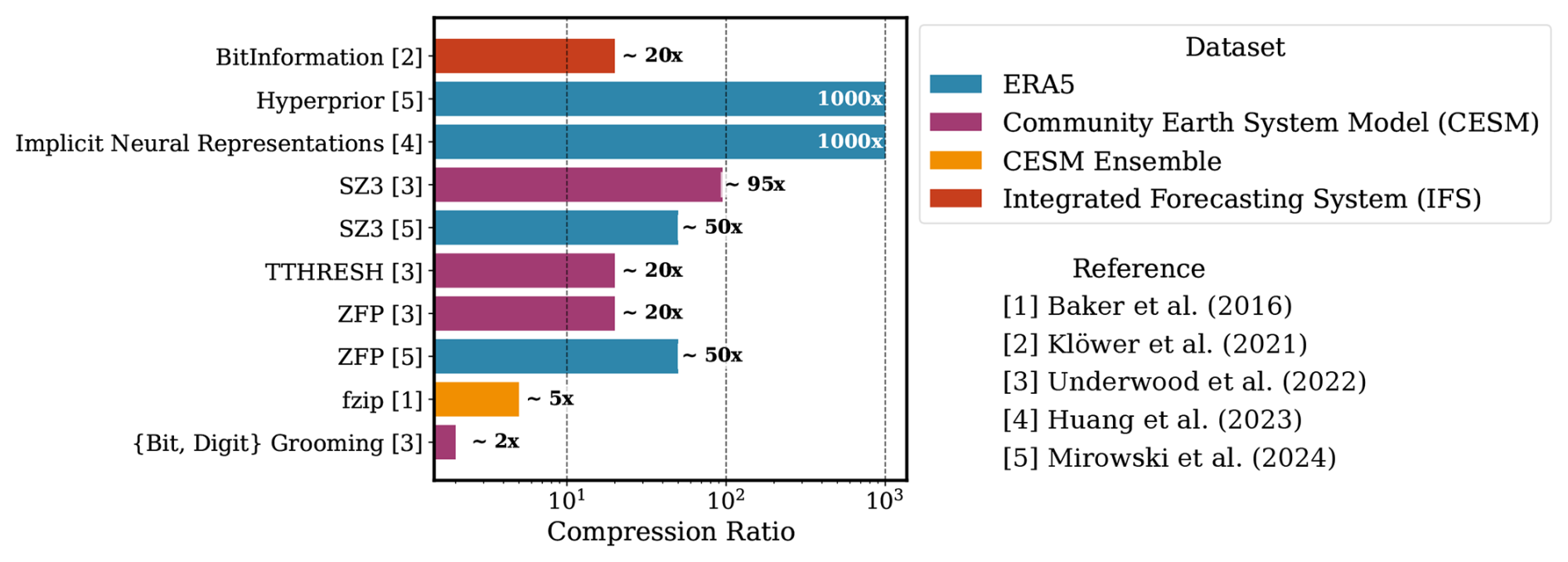
Figure 1 Compression ratios (uncompressed size $/$ compressed size) of different compressors applied to climate data reported in the literature. There are large variations in the reported compression ratios due to differences in: the data sources and variables that are being compressed; the exact techniques used to compute the compression ratio; and the error tolerances. Overall, these differences make it difficult to directly compare the reported compression ratios.

Surveying the literature on lossy compression for climate data, we find that the lack of a common benchmark makes it difficult to rigorously compare the performance of different compression algorithms. Figure 1 provides an overview of the different compression ratios as reported in published works. Even for the same compressor, different studies may report drastically varying compression ratios because different datasets, different error metrics, or very different levels of a tolerable compression error are being used. Even the way that the compression ratio is measured can change between authors. Some directly measure the size reduction in the binary data of the data fields, while others measure the difference in the final file size on disk, making the compression ratio dependent on the used file format.

To provide a standardized framework for comparing compression algorithms, we therefore present ClimateBenchPress, a novel climate data benchmark for compression algorithms. The benchmark contains data on structured grids from a variety of input sources covering land, ocean and atmospheric variables of the Earth system at different spatial and temporal resolutions. Crucially, the benchmark comes with a pre-defined list of error bounds for each input variable that provides a guideline to make compression performance comparable. These error bounds are calculated with an automated algorithm and validated against bounds provided by experts. The code for data processing and evaluation procedures is fully open source and easily extensible, allowing users to add new data sources, compressors, or evaluation metrics.

In summary, our contributions are:

• Introducing ClimateBenchPress, a standardized open-source benchmark to evaluate the performance of lossy compression algorithms on climate datasets, available at https://github.com/ClimateBenchPress (last access: 2 July 2026).

• Evaluating an initial set of baseline compressors on ClimateBenchPress to provide a reference for the compression performance that downstream users can expect in practice.

• Discussing the trade-offs between different compressors, providing actionable insights for compression users. Namely, compressors based on bit rounding or stochastic rounding achieve modest compression ratios of around 10 but they are very robust to failures. More advanced compressors can reach higher compression ratios but they are more prone to fail on edge cases so they require more careful use-case specific validation. Compressors generally have limited support for pointwise relative errors and different compressors might use slightly varying definitions of “relative” which end users should be aware of.

2 A Benchmark Dataset for Evaluating Climate Model Compressors

2.1 Compression Tasks

The goal of the benchmark is to provide data that comes in the form of multi-dimensional arrays $X\in {\mathbb{R}}^{T\times N_{\left(\mathrm{lon}\right)}\times N_{\left(\mathrm{lat}\right)}\times L\times V}$ with T giving the number of time steps, N_(lon) the number of longitude coordinates, N_(lat) the number of latitude coordinates, L the number of vertical levels, and V the number of variables/fields. Crucially, $T,N_{\left(\mathrm{lon}\right)},N_{\left(\mathrm{lat}\right)},L$ and V are all allowed to vary across datasets and not assumed constant. Hence, compression algorithms for this benchmark need to be able to deal with multiple grid resolutions in space, time, and number of variables. Lossy compression algorithms encode the data into a compressed representation such that, after decoding, the reconstructed array $\widehat{X}$ is an approximation to the original input, i.e. $X\approx \widehat{X}$.

For the purpose of this benchmark, we made the simplifying assumption that all data is defined on regular longitude-latitude grids. Of course, there are many data sources which do not natively lie on a regular grid, with many ESMs using their own unstructured grids. Regridding the data to a regular grid before passing it to a compressor is a common choice to deal with unstructured grids, hence measuring the performance of lossy compressors on regular grids still provides a useful signal for performance on unstructured grids. Moreover, many scientific compressors implicitly or explicitly assume a regular grid and therefore perform better if the input is transformed to a regular grid. However, the regridding from unstructured to regular grids is often a lossy process in itself that can affect the downstream compression performance, with the exact behavior depending on the details of the source and target grids, the regridding algorithms, and the variables that are being regridded. How to generalize compressors to arbitrary unstructured grids is still an open research problem, and outside the scope of this benchmark, as the additional complexity conflicts with the comparability we want to achieve. Similarly, there exist many relevant data modalities that do not lie on a structured grid, e.g. data from weather stations, weather balloons, ocean drifters or satellite swaths. Designing compressors for these modalities can require fundamentally different design decisions, which is why we exclude them here.

To keep the results of the benchmark easily interpretable, we only include a small representative subset of all available variables in climate data sets in this benchmark. Furthermore, we restrict the overall size of the benchmark dataset to relatively small subsets of data so that it can be easily downloaded onto a researcher's laptop. When selecting the input datasets and variables for our benchmark, we ensured that they cover the various dimensions of the climate data compression problem, including: varying spatial resolution (100 m to 150 km); varying temporal resolution (hourly to monthly); variables with a single vertical layer and variables with multiple vertical layers; data generated from a diversity of numerical models and from observations; different statistical distributions induced by different variables; different aspects of the Earth system, including land, ocean, and atmosphere variables. The specific datasets and variables in the benchmark, chosen to span the aforementioned dimensionalities of the compression problem, are:

• Sea-level Pressure, 10 m Wind Vector, and Humidity from the Integrated Forecasting System (IFS). Crucially, we use uncompressed IEEE-754 Standard 64-bit floating point outputs (https://apps.ecmwf.int/ifs-experiments/rd/hplp/, last access: 2 July 2026) The IFS model underpins the popular ERA5 reanalysis dataset (Hersbach et al., 2020) but this data distributed through the Copernicus Climate Change Service (C3S) Climate Data Store has already been compressed using GRIB's internal linear quantization that encodes floating point data into 24-bit unsigned integers (Dey et al., 2007; Klöwer et al., 2021).

• Air Temperature from the Coupled Model Intercomparison Project Phase 6 (CMIP6) (Eyring et al., 2016) as 4-dimensional datasets including the vertical and time dimension. Notably, the data also contains NaNs due to topography;

• Sea Surface Temperature (SST) fields from CMIP6 contain large regions of NaN values, due to SSTs being undefined on land, providing a significant challenge to compression algorithms.

• Precipitation and Outgoing Longwave Radiation (OLR) fields from the Next Generation Earth Modelling Systems (NextGEMS) project (Koldunov et al., 2023; Wieners et al., 2024; Segura et al., 2025) contain data from high-resolution km-scale climate models. The OLR – heavily impacted by the presence of clouds – and precipitation fields provide a test of whether compression algorithms can preserve high-frequency information and zero values in the input.

• Nitrogen Dioxide reanalysis data from the Copernicus Atmospheric Monitoring Service (CAMS) includes anthropogenic sources from industrial activity and transportation in the form of visual artifacts such as tracks and point emissions (Inness et al., 2019). We use CAMS data that is stored in 32-bit floating point precision and has not undergone any other compression (https://apps.ecmwf.int/ifs-experiments/rd/hej6/, last access: 2 July 2026).

• Above-Ground Biomass (AGB) (Santoro et al., 2024) as captured by the European Space Agency's Climate Change Initiative is a measure of the total weight of all living trees in a unit area. Derived from a multitude of satellite observations and provided at a resolution of 100 m, it is relevant to climate modeling, as forests are a major source and sink of atmospheric CO₂.

Table 1 succinctly summarizes the different data sources and their dimensionalities, and Appendix A contains visualizations of the different data sources. Note that most of the data sources contain a single variable with V=1. This is motivated by the fact that most climate and weather datasets are currently stored in chunked representations with each variable being stored separately. While there are often strong correlations between different variables that a compressor might be able to exploit, for large archived datasets like ERA5 users will rarely want to download all variables at the same time but rather only a small subset of the variables. Therefore, it is important that compressors perform well in the single-variable compression case which is the main focus of our benchmark. Nevertheless, for compression developers wishing to explore cross-variable compression we include the IFS dataset with sea-level pressure and the 10 m north- and eastward wind components, as well as, the NextGEMS dataset with the precipitation and outgoing longwave radiation variables.

Table 1 Description of datasets contained in ClimateBenchPress. The total size of the evaluation set is around 2.72 GB in v1.0. Dimensions are given as time (T), longitude (N_(lon)), latitude (N_(lat)), vertical levels (L), and variables (V). The data source abbreviations are: Integrated Forecasting System (IFS), Climate Model Intercomparison Project Phase 6 (CMIP6), Next Generation Earth Modelling Systems Project (NextGEMS), Copernicus Atmospheric Monitoring Service (CAMS), European Space Agency's Climate Change Initiative (ESA CCI; observation).

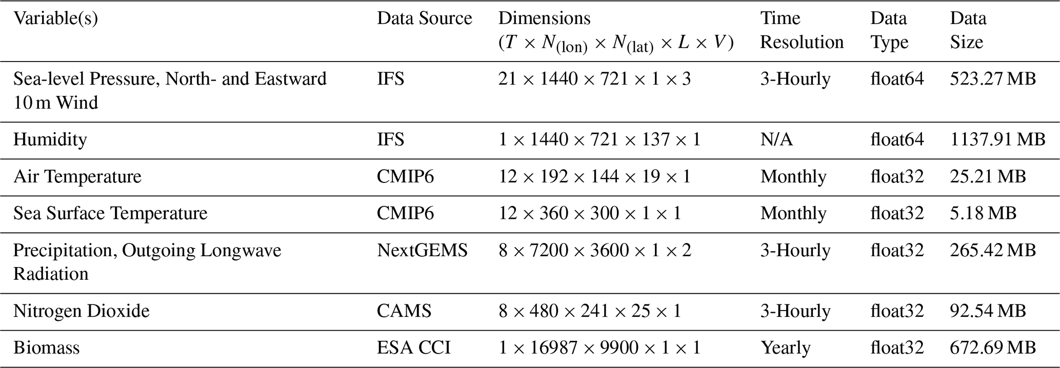
N/A – not applicable.

2.2 Error Bounds

Compression inherently involves trade-offs between different performance metrics: compression ratio (input data size divided by encoded size), speed, and error. If we are willing to tolerate a high error, we are able to compress more and vice versa. For example, just replacing all the input data in an array with their mean will lead to a high compression ratio – we only need to store a single floating point number, the mean, instead of the entire array – but will incur a large error. This is also known in the compression literature as the rate-distortion trade-off (Thomas and Joy, 2006).

Therefore, in designing our benchmark it is important to specify error bounds for each variable that the compressors should satisfy. Otherwise, compressors can report large compression ratios by allowing for large errors. Unfortunately, there are no well-defined, agreed-upon, standard error bounds for each variable. This is also largely due to the fact that the level of compression error that is tolerable is inherently application dependent, as mentioned in the introduction. Consequently, we do not select a single error bound but rather a set of three error bounds, which allows us to explore the Pareto front of optimal compressors, trading off higher compression ratios with higher errors. Some compressors achieve high compression ratios only with high errors, others produce low errors but consequently also lower compression ratios.

Additionally, we distinguish between pointwise absolute and relative error bounds.

Definition 1.

Let 𝔽_p denote the set of numbers representable with precision p in the IEEE 754 Standard for Floating-Point Arithmetic. For input data $X\in {\mathbb{F}}_p^{T\times N_{\left(\mathrm{lon}\right)}\times N_{\left(\mathrm{lat}\right)}\times L\times V}$, decompressed output $\widehat{X}\in {\mathbb{F}}_p^{T\times N_{\left(\mathrm{lon}\right)}\times N_{\left(\mathrm{lat}\right)}\times L\times V}$, and a variable index $\mathrm{0}\le v<V$, let X_i,v and ${\widehat{X}}_{i,v}$ denote the entries corresponding to the ith element obtained by flattening the first four dimensions (time, longitude, latitude, level) of X and $\widehat{X}$ onto a single axis. Then

1. the pointwise absolute error bound b_abs>0 is satisfied if $|X_{i,v}-{\widehat{X}}_{i,v}|\le b_{\text{abs}}$ or $X_{i,v}\equiv {\widehat{X}}_{i,v}$,²

2. the pointwise relative error bound b_rel>0 is satisfied if $|X_{i,v}-{\widehat{X}}_{i,v}|\le b_{\text{rel}}\cdot \left|X_{i,v}\right|$ or $X_{i,v}\equiv {\widehat{X}}_{i,v}$,

for all entries $i\in \mathit{\{}\mathrm{1},\mathrm{\dots },M\mathit{\}}$ with $M=T\cdot N_{\left(\mathrm{lon}\right)}\cdot N_{\left(\mathrm{lat}\right)}\cdot L$ denoting the total number of entries.

Relative error bounds are useful because absolute error bounds are not necessarily suitable for fields that vary largely in their magnitude, as e.g. many tracer concentrations. This specific formulation of the relative error bound also ensures it is defined for X_i=0, compared to the alternative formulation of the relative error bound in terms of $|X_i-{\widehat{X}}_i|/\left|X_i\right|$. Therefore, if the true value, X_i, is 0 then the pointwise relative error will only be satisfied if and only if the corresponding reconstructed value, ${\widehat{X}}_i$, is also 0. Importantly, there is no single, standard definition of the relative error convention in the compression literature and other relative error conventions might not be defined around 0 or do not require exact preservation of zeros. For example, the pointwise range-relative $/$ normalised absolute error which is defined as $|X_i-{\widehat{X}}_i|\le b_{\text{range-rel}}\cdot r$ with $r={max}_i{X}_i-{min}_i{X}_i$, denoting the range of the data, does not require exact preservation of zeros.

The type of bound we use for each variable is listed in Table 2. By default, we select an absolute error bound for each variable, but we resort to relative error bounds for the specific humidity, biomass, nitrogen dioxide, and precipitation variables, because these four variables have large variations in magnitude. Additionally, the biomass and precipitation fields contain many entries with 0s, and our definition of a relative error bound ensures that these values have to be preserved exactly.

Table 2 Individual error bounds for different input variables in ClimateBenchPress. Definition 1 describes the meaning of absolute and relative error bound, and Eqs. (1) and (2) define how the three different error bounds $b^{\left(\text{low}\right)},b^{\left(\text{mid}\right)},$ and b^(high) are computed in practice. “Non-Zero Range” indicates the smallest and largest non-zero absolute value, and the “Expert” column indicates bounds obtained by consulting domain scientists at ECMWF on what the maximum tolerable error for the variable should be, entries marked with an asterisk (^∗) are average rather than point-wise error bounds. Conventional abbreviations for variable names in parentheses.

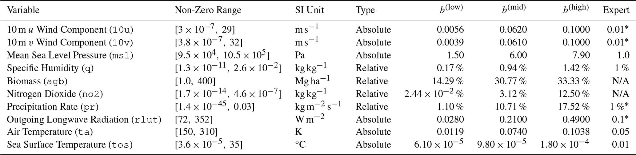
N/A – not available.

Rather than selecting the error bounds for each variable by hand, we leverage an automated mechanism that relies on the uncertainty information derived from the official ensemble statistics published along with ERA5 (Hersbach et al., 2020), which are based on a reduced resolution 10-member ensemble that incorporates the uncertainty from the data assimilation process and the physics parameterizations. The ERA5 ensemble data provides an ensemble mean μ_i,v and ensemble spread σ_i,v for variable v at grid point i, where the index i ranges over the time, longitude, latitude, and level dimensions³. Hence, $\mathit{\{}{\mathit{\sigma }}_{i,v}{\mathit{\}}}_{i=\mathrm{1}}^M$ for $M=T\cdot N_{\left(\mathrm{lon}\right)}\cdot N_{\left(\mathrm{lat}\right)}\cdot L$ represents the collection of ensemble spread data for variable v over all time steps, latitude-longitude points, and a specific vertical level. For pressure-level (not single-level) variables, we first compute the error bounds for the 1000, 850, 500, and 50 hPa levels as below and then use the average error bound for this benchmark.

For each variable, we compute three error bounds, $b^{\left(\text{low}\right)},b^{\left(\text{mid}\right)},$ and b^(high) that are based on the percentiles of the ensemble spread data $\mathit{\{}{\mathit{\sigma }}_{i,v}{\mathit{\}}}_{i=\mathrm{1}}^M$. These three bounds are meant to capture a variety of use-cases, from high error tolerance (e.g. visualization) to low tolerance (e.g. computing a function over the data). To derive absolute bounds, we use the 0 % (the minimum), 1 %, and 5 % percentiles of the non-zero ensemble spreads $\mathrm{\Theta }=\mathit{\left\{}{\mathit{\sigma }}_{i,v}\right|{\mathit{\sigma }}_{i,v}>\mathrm{0}{\mathit{\}}}_{i=\mathrm{1}}^M$, i.e.

$$\begin{array}{}\text{(1)}& \begin{array}{rl}& b_{\text{absolute}}^{\left(\text{low}\right)}=P_{\mathrm{0}\mathit{\%}}\left(\mathrm{\Theta }\right),b_{\text{absolute}}^{\left(\text{mid}\right)}=P_{\mathrm{1}\mathit{\%}}\left(\mathrm{\Theta }\right),\\ & b_{\text{absolute}}^{\left(\text{high}\right)}=P_{\mathrm{5}\mathit{\%}}\left(\mathrm{\Theta }\right).\end{array}\end{array}$$

Relative error bounds are calculated in a similar manner, with the only change that the ensemble spread values are normalized by the ensemble mean, again filtering out zero spreads and zero means ${\mathrm{\Theta }}^{*}=\mathit{\left\{}\right({\mathit{\sigma }}_{i,v}/{\mathit{\mu }}_{i,v}\left)\right|{\mathit{\sigma }}_{i,v}>\mathrm{0},\left|{\mathit{\mu }}_{i,v}\right|>\mathrm{0}{\mathit{\}}}_{i=\mathrm{1}}^M$ in

$$\begin{array}{}\text{(2)}& \begin{array}{rl}& b_{\text{relative}}^{\left(\text{low}\right)}=P_{\mathrm{0}\mathit{\%}}\left({\mathrm{\Theta }}^{*}\right),b_{\text{relative}}^{\left(\text{mid}\right)}=P_{\mathrm{1}\mathit{\%}}\left({\mathrm{\Theta }}^{*}\right),\\ & b_{\text{relative}}^{\left(\text{high}\right)}=P_{\mathrm{5}\mathit{\%}}\left({\mathrm{\Theta }}^{*}\right).\end{array}\end{array}$$

Intuitively, this process makes the heuristic assumption that variables with larger ensemble spreads require larger error bounds because there is more uncertainty in estimating their exact value.

The bounds for the sea surface temperature (ERA5 parameter name: sst), air temperature (t), outgoing longwave radiation (avg_tnlwrf), humidity (q), precipitation (avg_tprate), sea level pressure (msl), and wind vector variables (u10, v10) are all computed in this manner from the ERA5 ensemble data. For the biomass and nitrogen dioxide variable, there exists no matching ERA5 variable, and therefore, we revert to another mechanism to compute the error bounds. The biomass dataset also publishes standard deviation estimates, which represent the precision in the biomass point estimate, so we instead plug those standard deviations into Eq. (2) to compute relative error bounds. For nitrogen dioxide, we revert to using relative error bounds derived from the bitwise real information published in Klöwer et al. (2021), which are computed using information theoretic analysis.

Table 2 lists the exact error bounds we use for each variable. These bounds are not meant to represent general recommendations for which errors are tolerable or which error bounds should be used in practice. Instead, these bounds serve as a mechanism to enable a fair comparison of compression ratios. Users of lossy compression should always validate separately what error bound is acceptable for their specific use case.

To check whether the derived bounds are realistic, we additionally consulted domain scientists at ECMWF. Provided with existing errors from standard GRIB compression, the scientists drew on their experience with ERA5 data to specify the maximal absolute or relative errors they would consider acceptable. To not bias their judgements, scientists did not get access to the computed error bounds from Table 2. With this process, we were able to obtain “expert bounds” for the sea level pressure, humidity, precipitation, outgoing longwave radiation, air temperature and sea surface temperature variables. However, some of the expert provided bounds (marked with a ∗ in the table) are average rather than pointwise error bounds which can sometimes make a direct comparison difficult. Notably, pointwise error bounds are more conservative because they restrict the maximum pointwise error. In comparison to our computed bounds, the expert bounds mostly lie between b^(low) and b^(mid). The exceptions are the sea level pressure, specific humidity, precipitation, and sea surface temperature variables. For sea level pressure the expert provided bound (1.0 Pa) is just slightly below b^(low)=1.50 Pa. For specific humidity, the expert bound (1 %) is between b^(mid)=0.94 % and b^(high)=1.42 %. For precipitation the derived error bound of b^(low)=1.10 % is arguably more conservative than the the expert provided bound of 1 % because the derived error bound is a pointwise bound whereas the expert bound is an average bound. Hence, the expert average bound permits pointwise relative errors that exceed 1.1 % while the derived bound does not. The sea surface temperature variable is the only case for which the expert bound is multiple magnitudes larger than the derived bounds. They therefore provide bounds that are much more conservative. However, in general, the comparison to the expert bounds shows that our selected bounds are values that could realistically be picked in practice and are therefore suitable to be used as a base for comparing lossy compression algorithms.

2.3 Quantitative Evaluation Metrics

While the presented error bounds make the compression ratios between different compressors comparable, we still need a wider set of evaluation metrics to meaningfully compare their performance. As is standard in the compression literature, in this benchmark we will distinguish between two different types of evaluation measures: distortion metrics and compression metrics. Distortion metrics measure how much the reconstructed data differs from the original input, while compression metrics measure how much the data has been compressed and under what computational cost, e.g. encoding/decoding throughput. The next two sections introduce the specific metrics we compute as part of our benchmark. Notably though, our benchmark is easily extensible and users can readily add their own metrics for their own use cases.

2.3.1 Distortion metrics

Any distortion metric will only capture certain aspects of information loss, e.g. the maximum error bounds provided to the compressors do not take into account any spatial correlations of the errors, which is why we need multiple metrics to develop a more holistic picture of compressor performance. We selected the metrics so that each metric measures a distinct qualitative aspect of the compression performance. We purposefully made an effort to restrict the total number of metrics to avoid information overload when analyzing the benchmark results. Additionally, the distortion metrics need to be easy to understand for climate scientists, to help them inform their decision on which compressor to use in practice. Overall, the distortion metrics in the benchmark are as follows.

Mean absolute error (MAE) defined as $\frac{\mathrm{1}}{N}{\sum }_i|X_i-{\widehat{X}}_i|$ provides a measure of the average finite pointwise reconstruction error incurred by the compressor. Other metrics that are averages of pointwise errors, such as the peak signal-to-noise ratio (PSNR), could be used as well but we chose the MAE because it allows us to measure the error in the same units as the input data.

Maximum absolute error (MaxAbsError) defined as ${max}_i|X_i-{\widehat{X}}_i|$, provides a mechanism to investigate whether the provided error bound is exceeded for any data point, or not.

Spectral Error defined as $\text{SL}(X,\widehat{X})={\sum }_l{\left(S(X,l)-S(\widehat{X},l)\right)}^{\mathrm{2}}$ where S(X,l) denotes the radially averaged power spectral density (RAPSD) at wavelength l. This metric allows us to check whether the compressors preserve high-frequency signal information. We compute the RAPSD for each 2D latitude longitude field separately using the conventions of the pysteps library (Pulkkinen et al., 2019) making the simplifying assumption that the data lies on a Cartesian grid. For a field X of shape (N_(lon),N_(lat)), we apply the 2D discrete Fourier transform, shift the zero-frequency component to the array center, and form the squared-magnitude power spectrum normalized by the total number of grid points. S(X,l) is then defined as the mean of all power-spectrum values whose distance from the center equals l (rounded to the nearest integer). For data with multiple time steps and vertical levels, the SL error is computed for each 2D latitude longitude field independently and then averaged over all time steps and vertical levels.

Data Structural Similarity Index Measure (DSSIM) (Baker et al., 2023) aims to measure the visual similarity between the compressed and uncompressed data as it would be perceived by the human eye. Compared to pointwise error metrics it also takes into account the spatial correlations of the data. In particular, DSSIM is an adaption of the SSIM measure, which is widely used in the compression literature, to scientific floating point data. DSSIM is only defined on 2D fields, to be able to handle data with multiple time steps and vertical levels we follow the convention of Baker et al. (2023) and compute the DSSIM for each vertical level and time step separately, then take the minimum over vertical levels and average over time steps.

2.3.2 Compression Metrics

The standard measure to compare compression performance is the compression ratio, which is computed by dividing the size of the input data by the size of the encoding; hence, larger compression ratios are preferable because they correspond to smaller compressed files. For the benchmark we define the input data size as the number of bytes necessary to store the raw input arrays without any metadata. An input array $X\in {\mathbb{R}}^{T\times N_{\left(\mathrm{lon}\right)}\times N_{\left(\mathrm{lat}\right)}\times L\times V}$ with $M=T\times N_{\left(\mathrm{lon}\right)}\times N_{\left(\mathrm{lat}\right)}\times L\times V$ entries stored in 32-bit floating point precision will therefore be defined as having an input size of 4 ⋅ M bytes. This definition of the input size ensures that our compression ratio measurements are independent of the data format that is used to store the data and that we are measuring the pure compression performance of the compression algorithm and not the ability of a compressor to deal efficiently with a specific data format.

Another important aspect is the computational cost of applying a compressor, which we measure in two different ways. Firstly, for each compressor we keep track of the compression and decompression throughput, i.e. what is the wall clock time for compressing a fixed chunk of data? This metric is relevant because it allows us to extrapolate the time it would take to compress/decompress datasets of arbitrary size. On the other hand, raw throughput measurements are generally flawed because they are noisy and depend on the specific hardware and software environment which the benchmark code was executed in, including what other processes were executed at the same time. Hence, we additionally record the instruction count for both compressing and decompressing the data. Our benchmark ensures that the baseline compressors will reproducibly execute with exactly the same instruction counts on different machines. Therefore, instruction counts are a more objective measure of compressor complexity.

Similarly, other performance aspects such as memory usage or support for multi-threaded execution and hardware accelerators are often relevant in practice but are hard to measure objectively which is why we do not consider them here. Additionally, as most climate and weather datasets are stored in chunked representations, even compressors that only support single-threaded compression can easily be parallelized over large datasets by compressing separate chunks independently. Hence, the instruction count for single-threaded execution provides an objective first-order estimate of a compressor's computational cost and their relative ranking.

The prioritization between different compression metrics might also change depending on the different compression tasks, use cases, and compute and storage resources available. Not only that, but the prioritization between encoding and decoding complexity might change depending on the use case as well. For example, if we have a large archival dataset, such as ERA5, that gets accessed by thousands of users, then the compression ratio and decompression speed should be maximized. In this case, it is important that scientists are able to download and decompress the data quickly on their personal machines or institutional clusters. However, it is less important that the data can be compressed quickly because this only has to be done once. Therefore, compression times of multiple hours or even days might be acceptable. Of course, other use cases could have different priorities. For example, in operational weather forecasting, the time and computational resources that can be allocated to compression are constrained by the rate at which new forecasts need to be produced.

2.4 Implementation Details

All the code to download the data and reproduce the experimental results for the benchmark is accessible open-source at https://github.com/ClimateBenchPress. The data from the different sources outlined in Table 1 are converted into Zarr arrays (Miles et al., 2020) with canonicalised dimensions $V\times T\times L\times \times N_{\left(\mathrm{lat}\right)}\times N_{\left(\mathrm{lon}\right)}$ to provide a common data format for the benchmark. To compare a new compressor, the minimum requirement is that it can be made to compress a Zarr array (e.g. by individually compressing the numpy arrays for each variable), measure the byte size of the compressed representation, and output a Zarr array with the decompressed output. In the benchmark, we use the numcodecs (https://github.com/zarr-developers/numcodecs, last access: 2 July 2026) compression framework, which provides a minimal API for compressing n-dimensional arrays. To add a new compressor to the reproducible benchmark baseline, it must be wrapped inside a numcodecs codec.

For the results presented in this paper, we additionally wanted to ensure the fairness, reproducibility, and comparability of the performance of different compressors. To compress the input data, we use the numcodecs-wasm (https://numcodecs-wasm.readthedocs.io, last access: 2 July 2026) project, which adapts many popular scientific compressors to the numcodecs compression API (https://github.com/zarr-developers/numcodecs, last access: 2 July 2026). To guarantee cross-platform reproducibility, the numcodecs-wasm project compiles its compressors to WebAssembly bytecode inside an isolated Nix build environment and publishes them as pure Python packages that are compatible with the numcodecs API. WebAssembly (WASM) is a cross-platform bytecode format that was initially designed to safely execute compiled programs on web pages. Given its focus on security and cross-web-browser compatibility, WebAssembly is designed to facilitate performant and fully sandboxed execution (Spies and Mock, 2021). In our experimental evaluation, we use the Wasmtime (https://github.com/bytecodealliance/wasmtime, last access: 2 July 2026) WebAssembly reference engine. While the core WebAssembly instruction set is not entirely deterministic, non-deterministic instructions are very limited by design (WebAssembly Working Group, 2019), and any single-threaded core WebAssembly program can be transformed to have bit-reproducible execution. The WebAssembly 3.0 draft specification even defines a deterministic profile for this use case (WebAssembly Community Group, 2025). It is furthermore possible to instrument any WebAssembly program with a virtual bytecode instruction counter, which can be used as a deterministic, fully reproducible, user-space performance metric that does not suffer from measurement noise or platform differences (Binder and Hulaas, 2006). Since the Python packages provided by numcodecs-wasm ship with the pre-compiled cross-platform WebAssembly bytecode and only use deterministic instructions, the wrapped compressors execute exactly the same on any platform, thus allowing this benchmark to report reproducible, platform-independent, and noise-free results. Overall, the usage of numcodecs-wasm guarantees that, apart from wall-time execution speed measurements, all results and metrics are reproducible on any CPU architecture, from large HPC systems to interactive demonstrations on local machines.

For the comparison of the baseline compressors in Sect. 3, different variables are compressed separately. Evaluating different multi-variable compression approaches is left for future extensions to the benchmark.

3 Results

In order to gain an understanding of the current state of lossy compression algorithms for climate data, we evaluate a set of baseline compressors on ClimateBenchPress. For readers who are new to lossy compression, the presented results here should be seen as a helpful guideline for how to interpret the results of the benchmark and understand the different trade-offs involved when choosing between different codecs. For readers who are interested in using lossy compression for their own work, the results here can help narrow down the compressors they might want to consider. As mentioned earlier though, the benchmark is mainly designed to be a tool to compare different compressors and not to validate them. It is important that all users of lossy compression run their own use case-specific validations before applying lossy compression. This is especially important because different compressors can have substantially different qualitative behavior that can be hard to capture using general-purpose error metrics, as we will discuss in Sect. 3.3.

3.1 Baseline Compressors

As baselines, we mainly consider compressors that were specifically developed for floating-point data and scientific applications. A key feature of lossy compressors designed for scientific applications is a mechanism to control the maximum pointwise error (relative and/or absolute error) incurred during the compression process. Some compressors also support bounding the peak signal-to-noise ratio (PSNR) which also bounds the mean squared error. Bounding the pointwise absolute error is a stronger bound and therefore also bounds an average error but many compressors do not provide this as a specific control. A notable exception in our list of baseline codecs is the JPEG2000 codec, which was developed for image compression but has been increasingly applied to scientific data as well (Woodring et al., 2011; Silver and Zender, 2017; Pellicer-Valero et al., 2025). Since it has seen decades of development and continuous improvement, it can provide a reference point for what compression ratios may be possible with traditional compression schemes. For now, we have not included any neural compressors in the benchmark because they are either developed only for a specific dataset (Mirowski et al., 2024; Han et al., 2024), generally ERA5, or do not come with any built-in mechanisms to control their error bound (Huang and Hoefler, 2023). We hope this benchmark encourages developments in neural compressors that overcome these shortcomings. We now briefly describe our baseline compressors.

Bit Rounding (Zender, 2016; Delaunay et al., 2019) rounds the floating point mantissa to a specified number of bits. This gives a transparent mechanism to control the desired precision and relative error in the data and provides an interpretable mechanism for understanding what information is lost in the compression stage. Bit Rounding can bound the absolute error by varying the number of mantissa bits but this is not considered here. Similarly, Stochastic Rounding uses random noise to round the input data to the nearest specified decimal precision. The goal of the added noise is to avoid any systematic biases in the compressed data due to the rounding process, which can otherwise remove small gradients in the data. Stochastic Rounding can be formulated to round to a constant number of mantissa bits, effectively bounding a relative error but this is not considered here. We combine both Bit Rounding and Stochastic Rounding with a lossless compressor. For each rounding mechanism we will evaluate two choices of lossless compressors: Zstd, a widely used byte compression codec designed for web data, and PCO (Loncaric et al., 2025), a novel lossless compressor designed specifically for numerical data. SZ3 (Liang et al., 2022) is a prediction-based error-bounded lossy compressor that uses Lorenzo predictors (Ibarria et al., 2003) and spline-based interpolators to exploit local correlations in the input data; in our experiments we use version 3.2.2. EBCC (Huang et al., 2026) uses JPEG2000 as a base compression layer and uses residual encodings based on wavelet transforms and SPIHT (Set Partitioning In Hierarchical Trees) to ensure adherence to error bounds. ZFP (Lindstrom, 2014) instead decorrelates the data by applying an orthogonal transform to $\mathrm{4}\times \mathrm{\dots }\times \mathrm{4}$ sub-blocks of X. We additionally evaluate a more recent variant of ZFP called ZFP-ROUND (Hammerling et al., 2019) that reduced bias with an improved rounding mechanism for the transform coefficients based on feedback from the climate science community. JPEG2000 (Skodras et al., 2001) uses a wavelet-based transform to decorrelate the data and then quantizes individual entries in the transformed input space. JPEG2000 does not support floating-point data; instead, we linearly quantize the data to operate on integers. JPEG2000 does not provide a mechanism to bound the maximum pointwise error; instead, we convert the absolute or relative error bounds to peak signal-to-noise ratio (PSNR), which can be passed to the compressor as a target. Notably though, PSNR is a measure of the average rather than maximum error. Finally, SPERR (Li et al., 2023) is also a wavelet-based transform compressor but with the added feature of allowing for bounding the maximum pointwise error. The exact versions of the compressors that we tested in the benchmark are given in Table B1 in Appendix B.

Table 3 Supported types of error bounds for different compressors. The support for relative error bounds for EBCC, SZ3, ZFP, and ZFP-ROUND is in brackets because while these compressors have some mechanism to bound the relative error, we found in our experiments that they tend not to strictly adhere to the provided error bounds. In particular, the “relative” error bounds provided by EBCC and SZ3 are range-relative, not pointwise relative. Bit and Stochastic Rounding have errors in brackets as it is possible to reformulate these compressors towards these bounds which however is ignored here. Some compressors also support bounding the peak signal-to-noise ratio, PSNR. SZ3 is in brackets because it translates the PSNR bound into a pointwise absolute error bound internally.

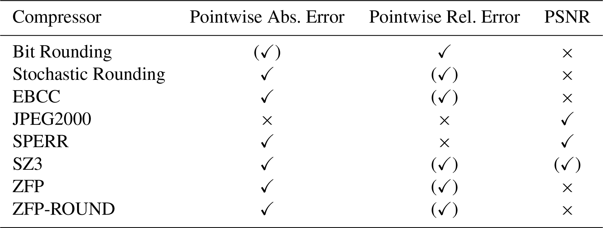
As highlighted in Table 3, most compressors do not have support for specifying both absolute and relative error bounds. Therefore, we sometimes need to convert between absolute and relative error bounds in order to use the error bounds from Table 2 for a specific compressor. Specifically, according to Definition 1, a pointwise relative error bound, b_rel, satisfies $|X_i-{\widehat{X}}_i|\le b_{\text{rel}}\cdot \left|X_i\right|$ for all indices i, whereas a pointwise absolute error bound satisfies $|X_i-{\widehat{X}}_i|\le b_{\text{abs}}$. For relative error bounds the right-hand side value of the inequality varies depending on the input value $\left|X_i\right|$, whereas the right-hand side value is fixed for the absolute error bound. To convert a relative error bound, b_rel, to an absolute error bound, we find the smallest non-zero right-hand side value that appears in the dataset, i.e. $b_{\text{abs}}^{\prime }={min}_i\left|X_i\right|\cdot b_{\text{rel}}$, where the minimum is taken over all non-zero values. Similarly, to convert an absolute error bound, b_abs, to a relative error bound $b_{\text{rel}}^{\prime }$ we want to ensure that every possible right-hand side value of the inequality is bounded by the original absolute error bound, i.e. $b_{\text{rel}}^{\prime }\cdot \left|X_i\right|\le b_{\text{abs}}$ for all i, which is satisfied by picking $b_{\text{rel}}^{\prime }=b_{\text{abs}}/\left({max}_i\right|X_i\left|\right)$.

These error bound transformations are intentionally quite conservative, meaning that if a compressor only supports absolute error bounds, passing $b_{\text{abs}}^{\prime }$ as an error bound will ensure the original relative error bound is satisfied on all non-zero entries. At the same time, if the input data has many near-zero or subnormal values the converted absolute error bound $b_{\text{abs}}^{\prime }$ might be very restrictive. Other approaches to converting relative to absolute error bounds and vice versa are feasible, e.g. Liang et al. (2018) describe an alternative method for bounding the ratio-relative error using a logarithmic transform.

Overall, if an error bound transformation was applied for a compressor, the achieved compression ratios should be seen as a conservative lower bound estimate and higher compression ratios could be achievable if a more permissible error bound transformation is used. Both the SZ3 and the EBCC compressor allow the user to configure a relative error bound. However, they use a range-relative error (as defined in Sect. 2.2) which in most cases is less strict than our pointwise relative error bound. To assess the impact of these different relative error bound definitions we also consider the two compressor variants SZ3-Abs and EBCC-Abs that do not use the built-in relative error functionality of these compressors. Instead these variants convert all pointwise relative errors to pointwise absolute errors using the conservative transform described above.

3.2 Quantitative Results

3.2.1 Scorecards

A single evaluation sweep over all baseline compressors, input variables, error bounds, and evaluation metrics produces a large set of results that can be difficult to analyze. Our two main tools to summarize our benchmark results will be: (1) Scorecards, inspired by their use to evaluate different forecasting models at ECMWF (https://sites.ecmwf.int/ifs/scorecards/, last access: 2 July 2026) and in WeatherBench (Rasp et al., 2024); and (2) rate-distortion plots, which are common in the compression literature.

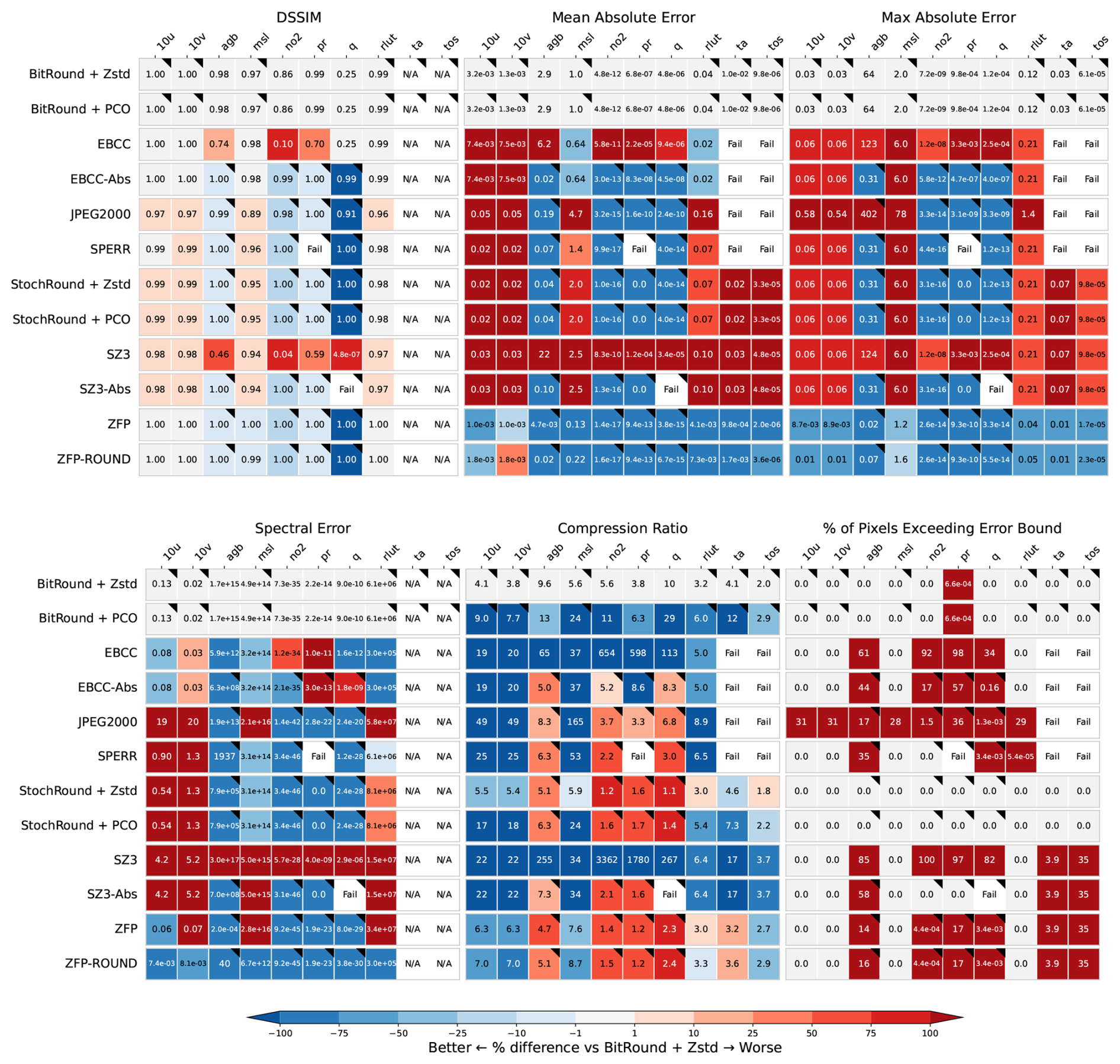
Figure 2 Overview scorecard summarizing the benchmark results. Each panel shows a different metric, each row a different compressor, and each column a different variable. Black triangles indicate compressor-variable pairings for which an error bound transformation was used. The scorecard allows us to compare the performance of compressors across different metrics: for example, SZ3 provides uniformly high compression ratios but sometimes exceeds the provided error bounds and leads to generally higher average errors. This scorecard shows the specific metrics evaluated on the “mid” level error bound; scorecards for the other error bounds are listed in Appendix C. “Fail” entries denote cases in which running the compressor raised an error. We exclude DSSIM and Spectral Error metrics for “ta” and “tos” variables, indicated by “N/A” entries, because these metrics are not robust to large regions of NaN values. See Table 3 for variable abbreviations.

The scorecards in Fig. 2 provide a quick visual overview of which compressors perform well in the different performance metrics. The wavelet-based compressors JPEG2000, SPERR, and EBCC are all able to achieve large compression ratios but they behave differently in how they control errors. JPEG2000 tends to fail the provided error bound as it has no in-built mechanism to constrain the pointwise error. SPERR does not always adhere to the error bound due to known issues in encoding the error bound correction (Fallin and Burtscher, 2024). EBCC tends to provide smaller average errors compared to SPERR but often fails on relative error bounds which is discussed more below. SZ3 is also able to provide compression ratios that are often on the same order of magnitude as those of the wavelet-based compressors. However, the benchmark also exposes some interesting failure cases for SZ3 v3.2.2. For example, both the air and sea surface temperature variables (“ta” and “tos” columns in the scorecard, respectively) contain NaN values in the input data, but instead of preserving these NaN values, SZ3 fills in these regions in the input data with interpolated numerical values.⁴ ZFP and ZFP-ROUND exhibit the same failure case, which is especially problematic because it is a silent failure; no error was raised during the compression process. JPEG2000 and SPERR fail on NaN inputs as well, but they raise an error instead of infilling any values⁵. In the case of JPEG2000, the failure can be attributed to the quantisation from floating-point numbers to integers, which does not account for NaN values.

Additionally, many compressors struggle to strictly adhere to relative error bounds; see Table 2 for the list of variables with relative error bounds. As discussed in Sect. 3.1, SZ3 and EBCC use alternative definitions of relative errors which leads to large percentages of pixels exceeding the error bound. The SZ3-Abs variant that utilises the conservative relative to absolute error transformation mostly remedies this issue, however it still fails on inputs that require preservation of 0 values⁶. The EBCC-Abs variant reduces the failure rate for relative error bounds but still has a singificant percentage of pixels not adhering to the bound. ZFP, ZFP-ROUND⁷, and SPERR also struggle with relative error bounds as they all fail to preserve 0 values , e.g. above-ground biomass is zero over the ocean but compressed here to non-zero values⁸.

Even Bit Rounding fails to adhere to the relative error bound on the precipitation data. Upon investigation of the ICON precipitation data, we identified that the failure is due to subnormal floating-point numbers being present in the ICON data. Bit Rounding fails to adhere to the error bound because the implementation that we are using computes the number of mantissa bits to keep as $k=-\lfloor {\log }_{\mathrm{2}}\left(b_{\text{rel}}\right)\rfloor -\mathrm{1}$ from the relative error bound b_rel, but this formula fails to hold for subnormal values. This failure case provides an illuminating example of why we need rigorous evaluation checks for lossy compressors. In many ways, this is a benign failure. The values are so small, smaller than $\approx \mathrm{1.1754942107}\times {\mathrm{10}}^{\mathrm{-}\mathrm{38}}$ kg m⁻² s⁻¹, that they are physically implausible and a numerical artifact from the model. Furthermore, Bit Rounding will round these values to 0, so the impact on calculating any downstream statistics, e.g. total precipitation, will be insignificant. At the same time, exactly because these values are numerical artifacts from the model, it is important that lossy compression algorithms do not “mask/round away” these unphysical values, or at least make users aware of this special case. If this particular implementation of Bit Rounding were deployed in a way that all model outputs are lossily compressed before being written to disk, the model developers would have no way of knowing that the model produces subnormal values as outputs⁹.

In general, for variable and compressor combination that require a relative to absolute error bound transformation, we observe markedly lower compression ratios – this is true for the Stochastic Rounding, EBCC-Abs, JPEG2000, SPERR, SZ3-Abs, ZFP, and ZFP-ROUND compressors on the biomass (agb), nitrogen dioxide (no2), precipitation (pr), and humidity (q) variables. As noted earlier, this is due to the fact that we use a very conservative error bound transformation. Higher compression ratios could be achieved with a less conservative error bound transformation (e.g. Liang et al., 2018) or alternative relative error bound definitions, such as the range-relative error mentioned in Sect. 2.2.

Overall, our results demonstrate the need for a benchmark as a testing ground for compression developers. None of the failure cases of the compressors are necessarily difficult to overcome from an algorithm design perspective (failure on NaNs and adherence to relative error bounds), but the lack of an existing benchmark means that, currently, compression developers often do not consider these edge cases as requirements.

3.2.2 Rate-Distortion Plots

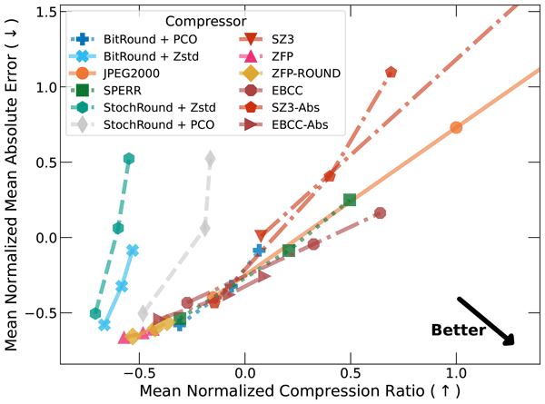
While scorecards provide a detailed overview of the compressor performance across different metrics and inputs, they make it difficult to visually assess the trade-off between compression ratio and distortion errors. Rate-distortion plots, as those shown in Fig. 3, allow us to assess exactly this trade-off. With rate-distortion plots, we can get an understanding of what compressors lie on the Pareto front of giving both high compression ratios and low levels of distortion, for different definitions of distortion. Normalization is applied to the compression ratios and error metrics for each variable, averaged across all datasets. This is done because different variables have different units and averaging their errors without normalizing would lead to the variables with the largest magnitudes dominating the average. Because the plotted quantities are averages, the rate-distortion plots in Fig. 3 should always be read in combination with the scorecards because even if a compressor does well on average across datasets there is still significant variation in their performance across the different datasets and variables. Specifically, for a set of metric values $\mathit{\left\{}{m}_{v,b,c}\mathit{\right\}}$ with input variable v, error bound b, and compressors c we compute the mean and standard deviation over all compressors and error bounds to obtain normalized scores as $n_{v,b,c}=(m_{v,b,c}-{\mathrm{mean}}_{c,b}(\mathit{\left\{}{m}_{v,b,c}\mathit{\right\}}\left)\right)/{\mathrm{SD}}_{b,c}\left(\mathit{\right\{}{m}_{v,b,c}\mathit{\left\}}\right))$. In Fig. 3 the normalized scores are for a given compressor and error bound averaged over all variables, i.e. $n_{c,b}={\mathrm{mean}}_v\left(\mathit{\right\{}{n}_{v,b,c}\mathit{\left\}}\right)$. These averaged normalized scores represent the average performance of a compressor relative to the other compressors. Values larger than 0 indicate that a compressor, on average across variables, achieves a larger score than the other compressors whereas a score below 0 indicates that the compressor achieves a lower score than the other compressors.

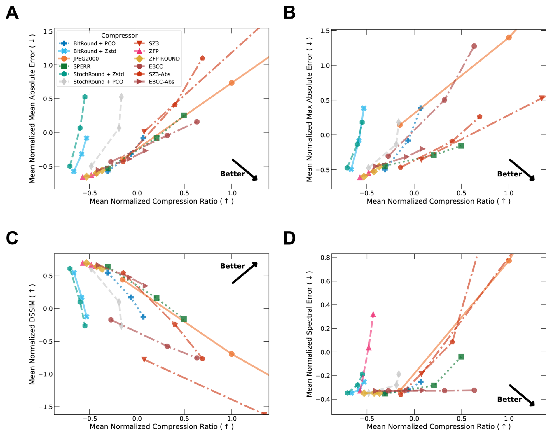
Figure 3 Rate-distortion plots for multiple distortion metrics: (A) normalized mean absolute error; (B) normalized maximum absolute error; (C) normalized DSSIM; (D) normalized spectral error, each on the y-axis, respectively. Normalization is applied to make compressor performances across metrics and datasets comparable, see text. Axes limits were selected to exclude outlier values; the high compression ratios of SZ3 and JPEG2000 are achieved through exceeding the provided error bounds. Appendix D shows the uncropped rate-distortion curves.

Figure 3 shows that SZ3 and the wavelet-based compressors (SPERR, JPEG2000, EBCC) generally provide the highest compression ratios across the different input variables. This, however, needs to be seen in the context of the results from the scorecards that showed these compressors often fail to strictly adhere to the provided error bound. Bit Rounding in combination with the PCO lossless compressor, “BitRound + PCO” in the plots, is surprisingly competitive and often provides compression ratios that are even competitive with more sophisticated compressors such as SPERR, despite the well respected error bounds. The notable jump in the compression ratios between “BitRound + Zstd” and “BitRound + PCO” highlights that we can still get quite significant improvements in the compression performance by using lossless compressors that are specifically designed for numerical data. Additionally, this makes a case for modular compressors, as the compression ratios are increased with no change to the lossy compression method and its errors. Overall, these results suggest that the simple combination of BitRound + PCO is a reliable and competitive alternative for users who are interested in not exceeding pointwise error bounds.

3.2.3 Instruction count

Finally, Fig. 4 displays the last aspect of compressor performance that we have left out so far: compression cost. We measure cost in terms of bytecode instruction count per encoded/decoded byte of data. We focus here on instruction count in favor of wall clock throughput measurements because the platform-independent bytecode instruction counts are reproducible between different CPU hardware architectures. Throughput measurements, on the other hand, tend to be noisy due to their dependence on, e.g. hardware details and what other processes are running on the same machine at the same time. Wall clock throughput measurements are shown in Fig. E1 in Appendix E¹⁰. EBCC is the most expensive compressor in encoding cost which is to be expected because it relies as JPEG2000, the second most expensive compressor for encoding, as a base compressor. This is a deliberate trade-off made by EBCC though because it was developed with the use on large archival datasets in mind that only need to be compressed once. Decoding time for EBCC is still competetive with the other compressors. Generally, encoding is more costly than decoding for all compressors except for both versions of ZFP. Both encoding and decoding costs are largely error independent. While some compressors, like ZFP, are known to be faster for very high error tolerances, within the provided error ranges low to high this is of little practical relevance. Even though Bit Rounding and Stochastic Rounding are simple lossy compression mechanisms, the lossless codecs PCO and Zstd add significant complexity to the entire compression procedure so that their compression cost is comparable to more complex lossy compressors such as SZ3, ZFP, and ZFP-Round.

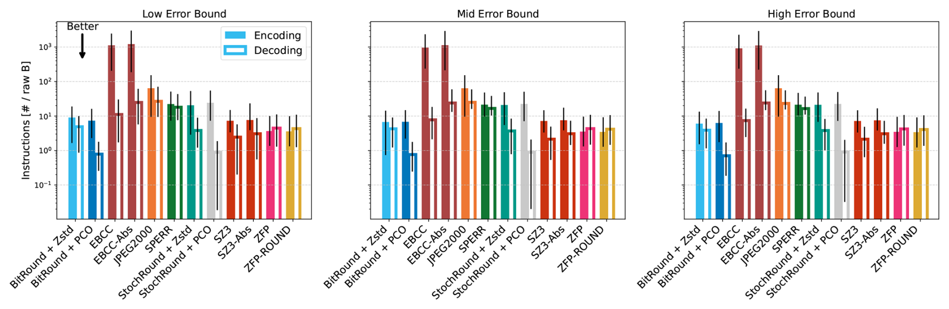
Figure 4 Comparison of encoding and decoding cost, measured in number of instructions per byte in the original data [# per raw B], for individual compressors and error bound levels. Solid bars indicate the encoding cost and hollow bars the decoding cost, bar height shows the median value across all variables and the uncertainty bars indicate the 25 % and 75 % quantiles. Note that the instruction count metric has no measurement noise – the variance only comes from the combination across several variables of different sizes. The instruction count in the JPEG2000 compressor currently does not include the cost of a per-element cast to float64 and uint32 during linear quantization preprocessing, which add two instructions per 4 (float32) or 8 (float64) bytes during both encoding and decoding.

3.2.4 Sensitivity of Compressor Performance to Chunking

As a default, we are passing the input data to compressors as a single chunk because of the relatively small overall size of our datasets; an exception is the humidity data which has 2 chunks by default because of its large size. Popular file formats, like NetCDF and Zarr, have explicit support for storing data in chunks, which allows for efficient access of subsets of large datasets because it avoids the need to load the full dataset into memory.

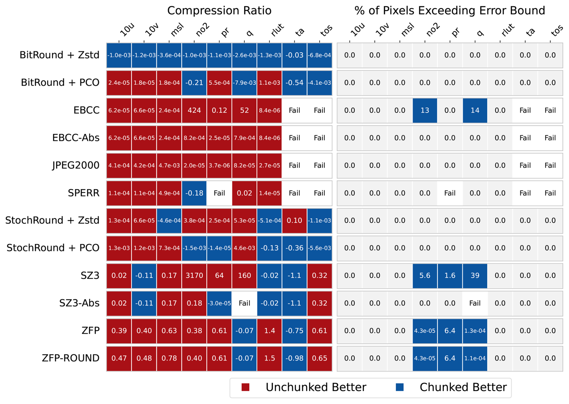
Figure 5 Difference in compression ratio and percentage of pixels exceeding the error bound between the unchunked and the chunked data. For a given metric, let m_nc denote the score for the data that is unchunked and m_c denote the score for the data that is chunked, then the scorecard here shows the difference $d=m_{\text{nc}}-m_{\text{c}}$. We exclude the above-ground biomass variable because the chunking algorithm keeps the whole dataset as a single chunk and therefore, the difference in the metrics is always 0.

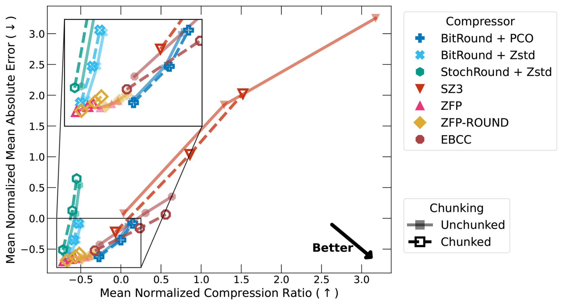
Figure 6 Impact of chunking on normalized mean absolute error and compression ratio. Hollow markers indicate results computed on chunked data and full markers with faded lines indicate results computed on unchunked data. The plot excludes StochRound + PCO, SPERR, EBCC-Abs, JPEG2000, and SZ3-Abs because for these compressors the visual difference is small. The plot with all compressors can be found in Appendix F.

As most climate datasets are stored in a chunked representation, we conducted a sensitivity analysis to study the impact that chunking has on compression performance. Determining good chunk sizes for a dataset is mainly application-specific because it depends on the typical access patterns to the data. Here, we chose a simple heuristic that ensures the chunk dimensions are roughly proportional and clean divisors of the full dataset dimensions. Additionally, the heuristic ensures each chunk is at least 4 MB in size, following recent guidance for CMIP7 datasets (Hassell and Cimadevilla Alvarez, 2025). The actual chunking used for each dataset is given in Table G1 in Appendix G.

Figures 5 and 6 show that the overall impacts of chunking on the compression ratio and mean absolute error are small. Across datasets and compressors, while overall for the majority of compressor-variable combinations the unchunked datasets provide marginally better compression ratios, for most compressors there is no uniform trend on whether chunking improves the compression ratio or not. Furthermore, the difference in compression ratios between the chunked and the unchunked data is generally <1, demonstrating that the overall effect is small. Even though the absolute change is small, for the ZFP and ZFP-ROUND compressors the impact of chunking is more significant because the base compression ratios are quite small so even small absolute changes have a noticeable impact. Further, on variables with a relative error bound, the EBCC and SZ3 compressors have large absolute changes. This is due to the aforementioned fact that EBCC and SZ3 internally transform the relative error bound into an absolute error bound constraint with the relationship $b_{\text{abs}}^{\prime }=b_{\text{rel}}\cdot ({max}_i{X}_i-{min}_i{X}_i)$. If the data is passed in chunks, the range of the data in the chunk, $({max}_i{X}_i-{min}_i{X}_i)$, will vary between chunks and therefore the compressors will in effect apply different error bounds to different chunks. This leads to the large observed difference in some compression ratios for EBCC and SZ3 in the nitrogen dioxide, precipitation, and humidity variables.

Overall, the impact of chunking on compressor performance depends on the specific characteristics of both the input data and the used compressor. Chunking has not been found to yield large improvements to compression ratios but remains attractive to parallelize the encoding across chunks. While we considered only one explicit chunking scheme here, we encourage benchmark participants to further explore different chunking choices and report how they affect compressor performance. For example, some chunking strategies might include artifacts at the chunk boundaries that could negatively affect the reconstruction error.

3.3 Qualitative Results

While the quantitative evaluation metrics from the previous section provide a good initial comparison of the different compressors, we found significant qualitative differences in the behavior of the baseline compressors.

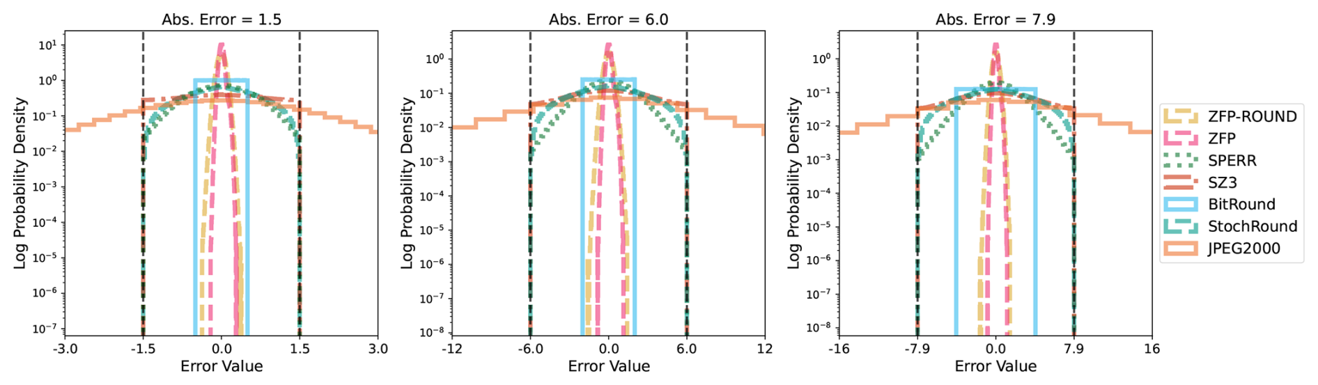
Figure 7 Error distributions for IFS sea level pressure for the three error bound levels. The black dashed vertical lines indicate the values of the error bounds. We do not differentiate between different combinations of StochRound and BitRound with lossless compressors because, by definition, the lossless compressors do not change the error distribution. Similarly, EBCC-Abs and SZ3-Abs are omitted because they behave identically to EBCC and SZ3 in this case.

Error Distributions. Different lossy compressors generally have different pointwise error distributions, as highlighted previously in e.g. Lindstrom (2017). Figure 7 illustrates the distribution of pointwise errors for the IFS sea level pressure variable, revealing that different compressors lead to substantially different error distributions. Compressing data with SZ3, SPERR, and StochRound leads to roughly uniform error distributions within the provided error bound; this also explains why in the scorecard in Fig. 2, these compressors often produce higher mean and maximum absolute errors. A uniform error distribution theoretically increases compression ratios compared to distributions with tails (e.g. SPERR or EBCC) as compressors can exploit the full range of the provided error bounds.

EBCC, ZFP and ZFP-ROUND tend to lead to roughly normally distributed errors (Lindstrom, 2017). The distributions of ZFP and ZFP-ROUND are significantly more concentrated around 0 though compared to EBCC, out of the three only EBCC exploits the full error bound range. Our implementation of BitRound relies on the conservative transformation of absolute to relative errors mentioned in Sect. 3.1 which leads to fairly conservative error distributions. The range of values in sea level pressure is less than a power of 2 (typically not exceeding 900–1100 hPa), so bounding the relative error easily bounds the absolute error too. A clear outlier is JPEG2000 because it has a much wider error distribution exceeding the bounds due to only optimizing for a global average error, as discussed before.

The heterogeneous error distributions further emphasize the need for compression users to conduct their own application-specific validation procedures, for example, by considering the errors in compressing the tails of the input data distribution or by applying statistical tests on whether the input and output distributions of the data match. Whether one shape of error distribution is preferable to another is again very use-case specific but compression users should be aware of the differences in behavior. This also highlights the fact that rather than fixing an error bound for a given variable ahead of time, users might want to explore the compression behavior under different error bounds and consider custom error metrics.

NaN Behavior. We mentioned in Sect. 3.2 that several compressors struggle on inputs that contain NaN values. In particular, EBCC, JPEG2000 and SPERR raise errors and refuse to compress any data with NaN entries. EBCC and SPERR are the only compressors that do this natively; the JPEG2000 failure is caused by our wrapper when converting the input floating-point data to integer data (JPEG2000 was not designed to work with non-integer data). As shown in Fig. 8, the SZ3, ZFP, and ZFP-ROUND compressors actually replace some of the NaN values with finite floating-point values. In the case of SZ3, the values are smooth interpolations of the sea-surface temperatures. While the differences clearly stand out for sea surface temperature fields, this behavior might be more difficult to spot if the input fields only contain a small number of NaN values, e.g. when representing temporarily missing observation values. Similarly, ZFP infills some finite floating-point values at the edges of NaN boundaries.

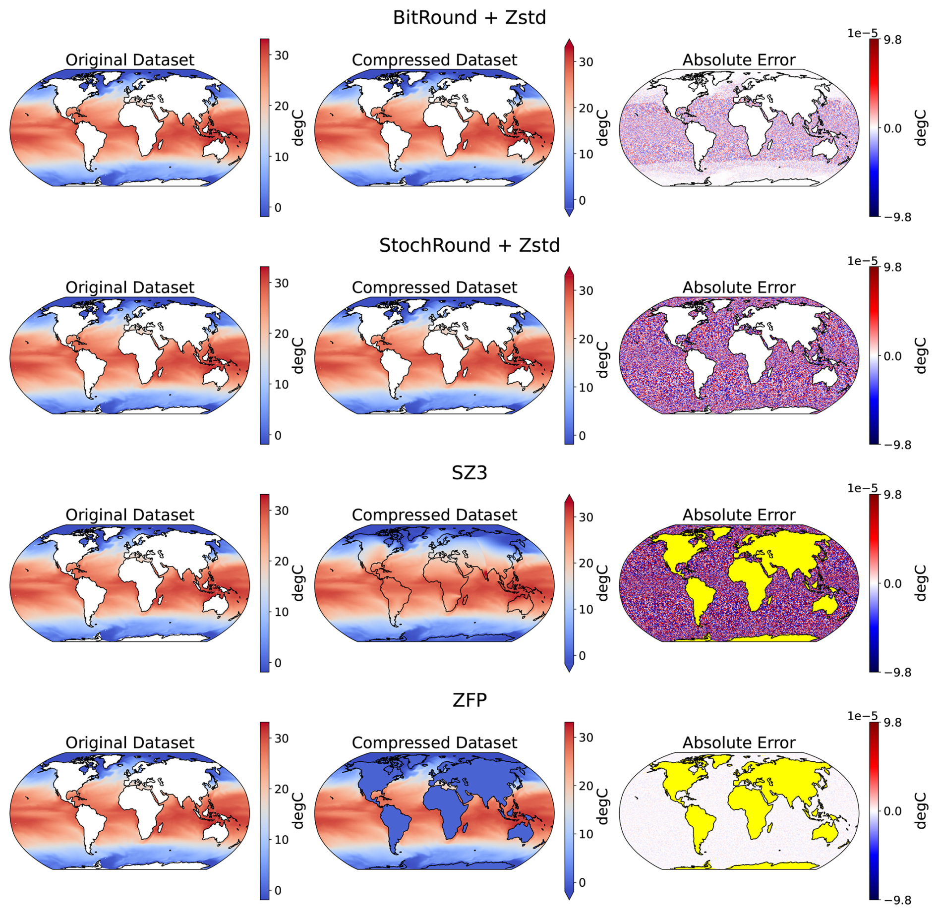
Figure 8 CMIP6 Sea Surface Temperature Errors. Original input field (left column), decompressed field (middle column), absolute error (right column) for different compressors (rows). SPERR, EBCC, and JPEG2000 are excluded here because they fail due to the presence of NaNs. We also only show one of the lossless compressors combined with rounding because, by definition, the lossless compressors do not change the error patterns. Yellow indicates regions where input values are NaNs but the compressor produces non-NaN values. Note that ZFP errors are non-zero but significantly below the error bounds; best viewed digitally.

Spatial Distribution of Errors. Figure 8 also demonstrates that the different compressors not only lead to different global error distributions, as shown in Fig. 7, the different compressors also have different spatial error patterns. Bit Rounding is implemented here to bound the relative error and therefore the magnitude of its reconstruction error will vary with the magnitude of the data, as we can clearly see in Fig. 8. The stochastic nature of Stochastic Rounding leads to noisier error distributions. As Stochastic Rounding is implemented here to bound an absolute error, the spatial distribution of its errors is uncorrelated white noise. For SZ3 and ZFP, the spatial error distribution is determined by their algorithm design. While there exist error metrics that explicitly take into account the spatial distribution of errors (Poppick et al., 2018), whether any given spatial pattern in errors is problematic is fundamentally dependent on the specific downstream analyses a user wants to conduct. It is therefore important for lossy compression users to run their own validation that is specific to their use case.

4 Conclusions

ClimateBenchPress addresses the need for a standardized benchmark of lossy compression algorithms for weather and climate data sets. The benchmark covers a diversity of different data sources (CMIP6, IFS, NextGEMS, CAMS, ESA CCI) with grid resolutions ranging from ∼ 100 m to ∼ 150 km. We select a small subset of variables from these data sources that cover land, ocean, and atmosphere components of the Earth system. For each variable in the benchmark, we derive quantitative error bounds with an automated algorithm that analyses the ensemble spread of each variable in the ERA5 ensemble. Our benchmark design keeps the total size of the input data at around 3 GB for easier evaluation and reproducibility, downloads to laptops, and compression without chunking on memory-constrained platforms.

Our evaluation of a set of twelve different compressor variants revealed that there are significant differences in their quantitative and qualitative performance. The benchmark uncovered edge cases that existing compressors struggle with, such as properly preserving NaN values. Bit Rounding in combination with the lossless compressor PCO generally respects error bounds and edge cases across different variables at modest compression ratios of around 10 and therefore is a robust compressor. Higher compression ratios are achieved by SZ3, JPEG2000, EBCC, and SPERR, often reaching compression ratios of 20–100 or more, but these compressors have various failure cases, which means care needs to be taken when they are applied in practice. Specifically, SZ3 silently filled in NaN values, a bug that has now been addressed due to our feedback, and struggles with relative error bounds; JPEG2000 does not provide support for NaN values or point-wise error bounds at all; and SPERR sometimes exceed the user-provided error bound. None of the technical issues are infeasible to fix, but their existence demonstrates the need for a robust benchmark to guide the development of compressors for climate data.

We emphasize that the benchmark is not intended as an exhaustive validation suite, but rather as a tool for assessing the comparative performance of lossy compressors. It is designed to expose the trade-offs that each compression algorithm makes and to provide an estimate of the rough order of magnitude compression ratio that users can expect in practice. The benchmark does not replace data- and model-specific validations of lossy compression algorithms. For example, as shown in Sect. 3.3, different compressors exhibit qualitatively distinct behaviors, often leading to varying spatial patterns in their errors, which has also been previously highlighted in the literature (Hammerling et al., 2019). Whether these spatial patterns are significant is inherently dependent on the specific analyses that users intend to conduct on the data.

We kept the total size of the benchmark dataset small to make it accessible to a wide variety of researchers. Furthermore, while many climate and weather datasets can exceed terabytes or even petabytes in scale, most datasets of that size are stored in a chunked representation with chunk sizes rarely exceeding 100 MB. Hence, even though our total benchmark dataset is small in size it still provides a useful testing ground for compressors because the task of compressing a large dataset will often reduce to compressing many small chunks. Nevertheless, an important avenue for future work is to provide an additional benchmark that challenges users to compress the full output of a high-resolution climate model run, possibly terabytes of data, and measure the maximum achievable compression ratio and key performance metrics. Such a benchmark would complement ClimateBenchPress because the sheer size of the output data creates its own set of engineering challenges (for example, optimizing I/O, exploiting hardware accelerators and parallelism, etc.).

ClimateBenchPress is intended to serve as a guideline for compression developers designing the next generation of algorithms. It serves as an honest and balanced review of currently available compressors and highlights difficulties when used for weather and climate data in practice. Many of the compressors evaluated here are still under active development, therefore our experimental results should only be seen as a snapshot of the compressor capabilities at the time of writing this article. This is why all code and data for ClimateBenchPress are openly accessible at https://github.com/ClimateBenchPress to enable anyone to run the benchmark whenever new compressor versions are released, and we specifically encourage compression developers to add their own compressors to the benchmark. The codebase is also easily extensible, allowing the addition of new data sources and metrics, thereby enabling the wider community to validate compression algorithms on their own datasets.

Appendix A: Sample Benchmark Data

Figure A1 Nitrogen Dioxide reanalysis data from the Copernicus Atmospheric Monitoring Service (CAMS). (A) pressure level 1000 hPa; (B) pressure level 500 hPa; (C) pressure level 1 hPa. Ship tracks and near-ground point sources are visible in (A), mid-tropospheric advection and mixing in weather systems in (B) and chemical processes in the stratosphere following solar radiation in (C).

Figure A2 Variables from the IFS dataset. (A) sea-level Pressure; (B) 10 m u component of wind; (C) 10 m v component of wind.

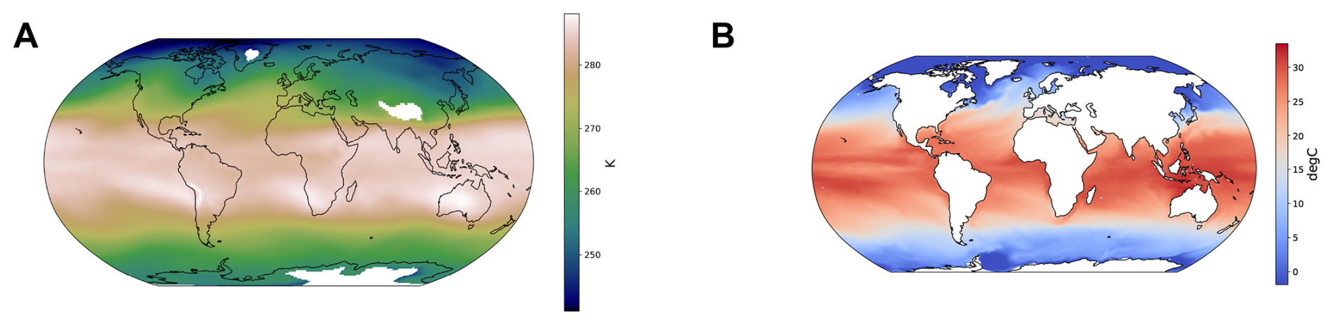
Figure A3 CMIP6 data for the ACCESS-ESM1-5 model. (A) air temperature at 700 hPa; (B) sea surface temperature.

Figure A4 Sample output fields from the ICON model in the NextGEMS intercomparison project. (A) outgoing longwave radiation; (B) precipitation.

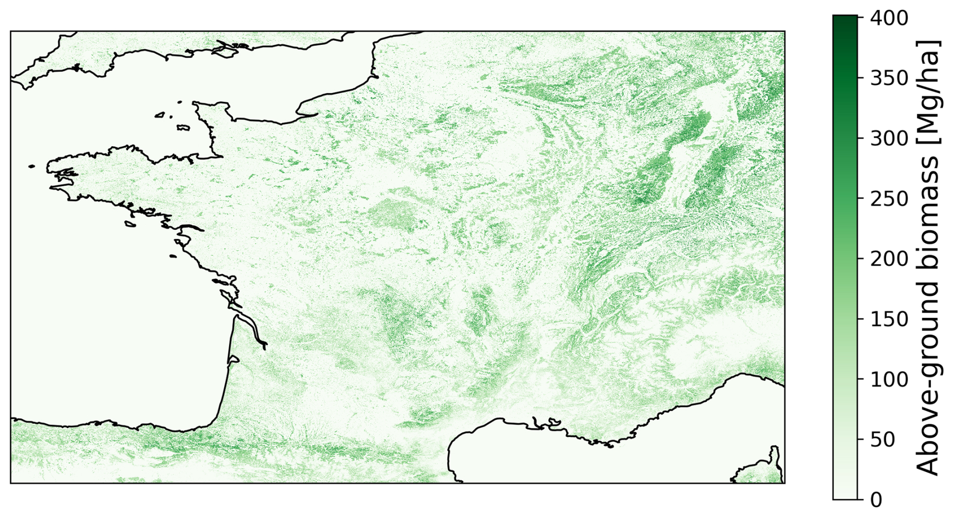
Figure A5 Sample output of the ESA above-ground biomass dataset covering France and adjacent countries.

Appendix B: Compressor Versions

Table B1 Versions of the compressors used in this benchmark. For each compressor, we provide the published version, if applicable, and the name and version of the corresponding numcodecs-wasm Python package. We use numcodecs-wasm version 0.2.2. The rounding-based compressors are widely reimplemented and no standard implementation exists.

Appendix C: Scorecards

Figure C1 Scorecard for the low error bound. Figure conventions as in Fig. 2.

Figure C2 Scorecard for the high error bound. Figure conventions as in Fig. 2.

Appendix D: Full Rate-Distortion Plots

Figure D1 Full Rate-Distortion curves for multiple metrics without the cropped axes: (A) normalized mean absolute error; (B) normalized maximum absolute error; (C) normalized DSSIM; (D) normalized spectral error. Conventions as in Fig. 3.

Appendix E: Throughput Measurements

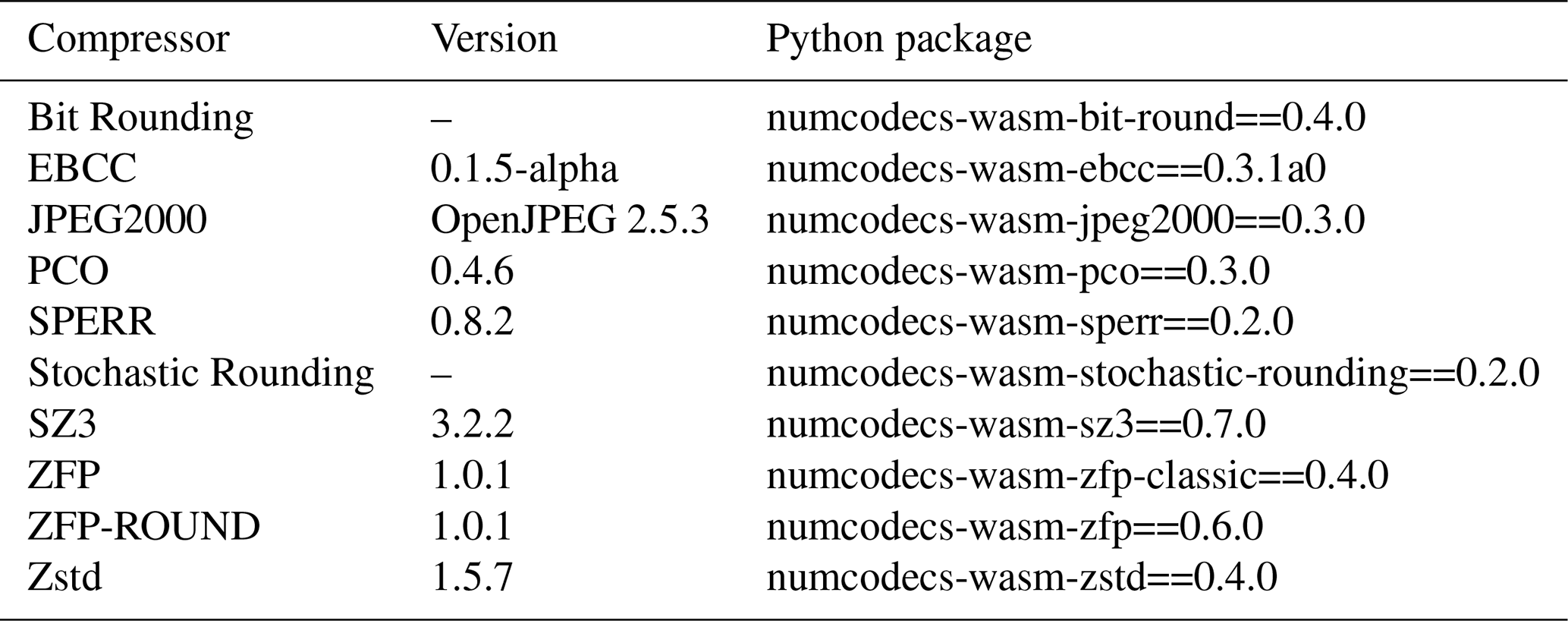
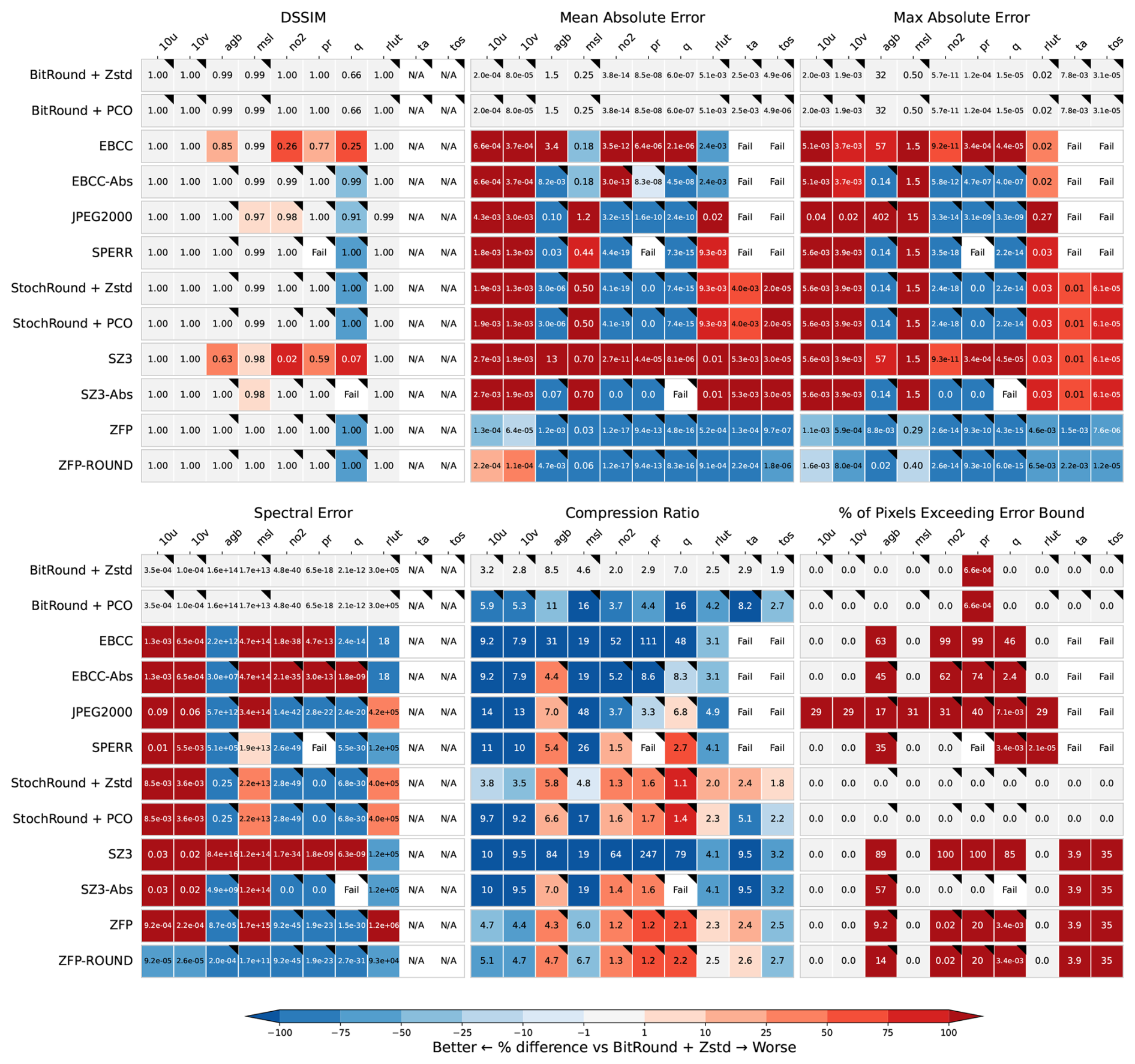
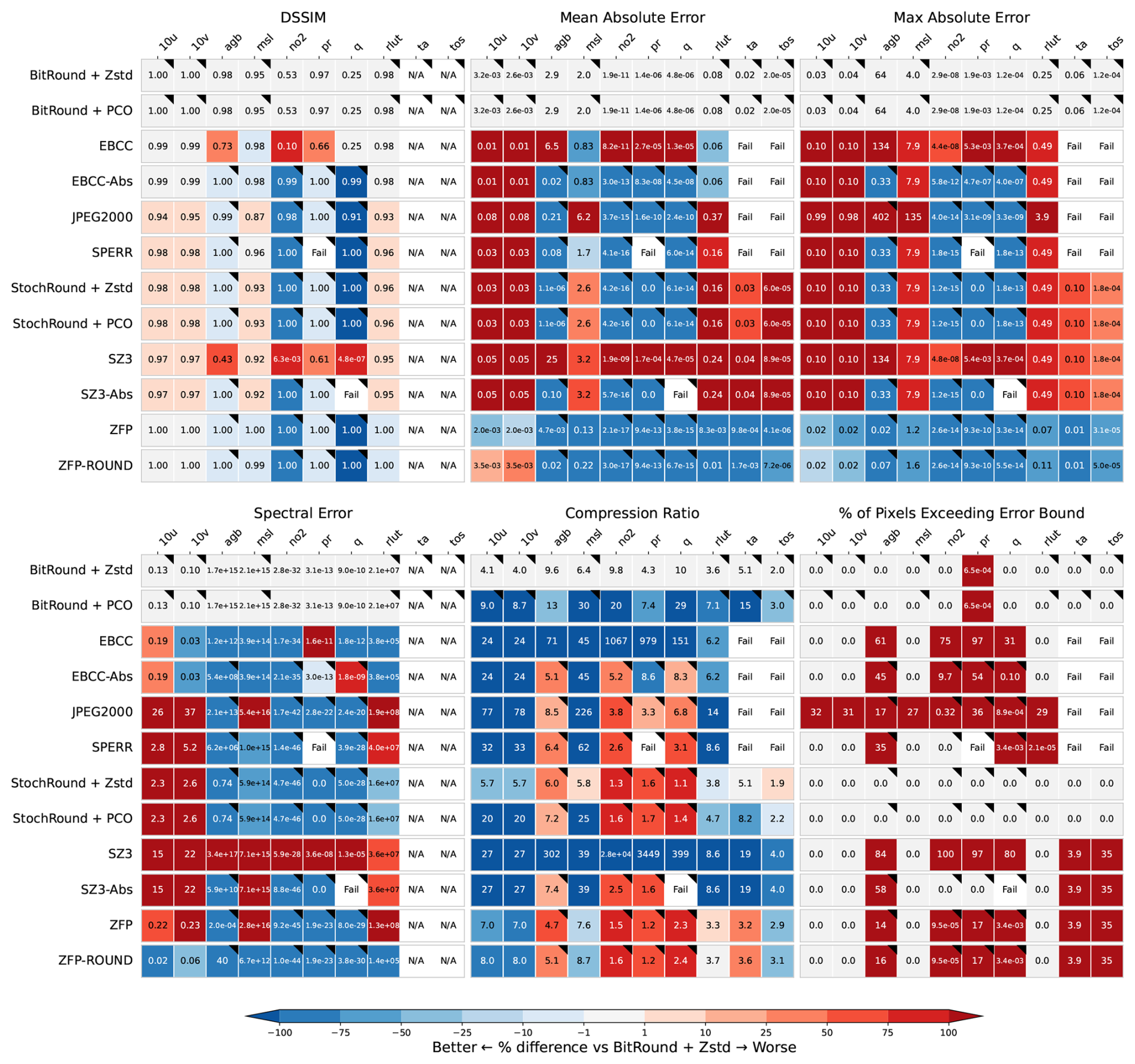
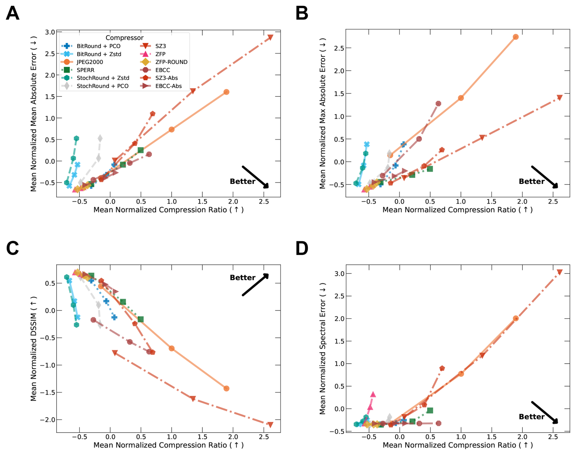
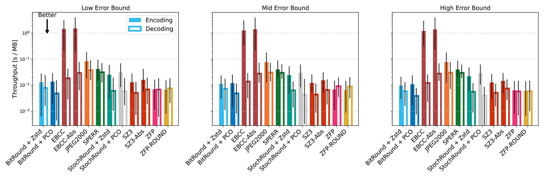
Figure E1 Comparison of encoding and decoding throughput, measured in [s MB⁻¹], for individual compressors and error bound levels. Solid bars indicate the encoding time and hollow bars the decoding time, bar height is showing the median value across all variables, and the uncertainty bars indicate the 25 % and 75 % quantiles. Measurements are run on a AMD EPYC 9654 CPU and utilize a single thread. Note that these throughput measurements should only be seen as a relative comparison. Our benchmarking code incurs a significant amount of overhead (Jangda et al., 2019) through the compilation to WebAssembly and to ensure reproducibility. Therefore, the numbers reported here should be seen as unoptimized, lower bound estimates of the throughput that might be achieved in practice.

Appendix F: Full Chunking Rate-Distortion Plot

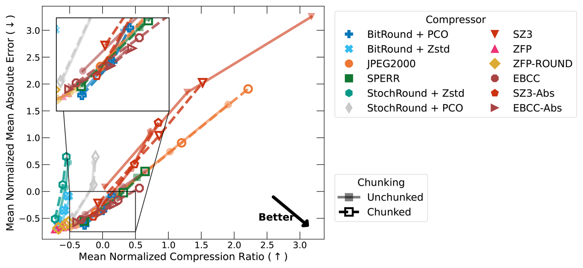
Figure F1 Impact of chunking on normalized mean absolute error and compression ratio. Hollow markers indicate results computed on chunked data and full markers with faded lines indicate results computed on unchunked data.

Appendix G: Chunk Sizes

Table G1 Chunk shapes used in the experiments from Sect. 3.2.4. Dimensions are given as time (T), longitude (N_(lon)), latitude (N_(lat)), vertical levels (L), and variables (V). “Chunk Size” reports the size of one chunk of a single variable under the computed chunking. “Total Size” reports the full size of the dataset. For “Chunked”, the bold numbers indicate the dimensions that have been chunked.

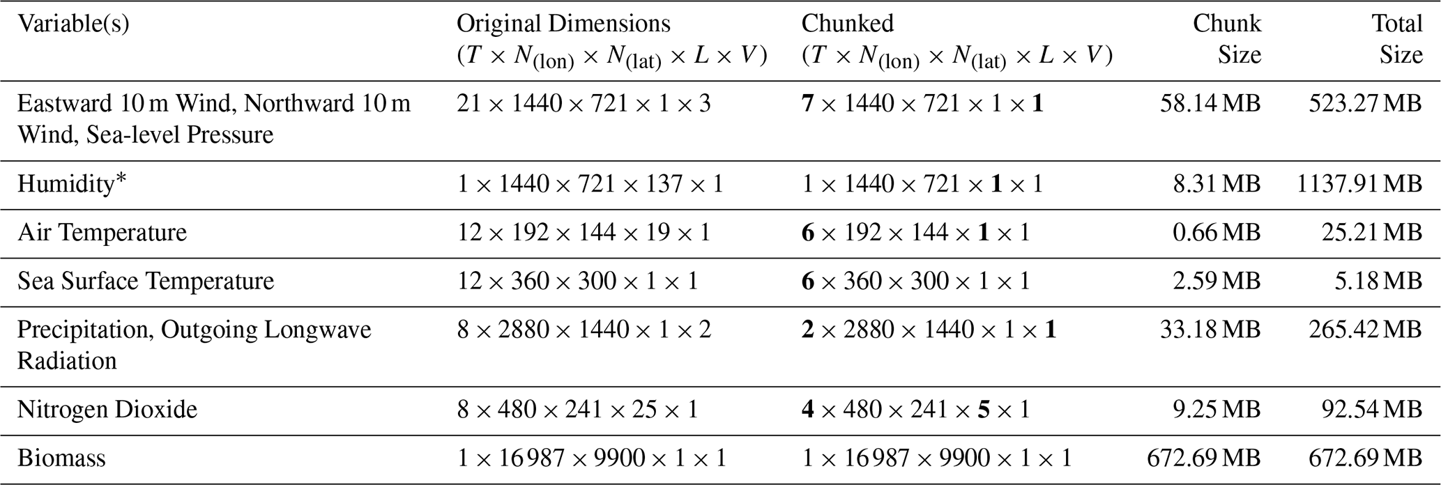
^∗ By default Humidity uses a chunking of $\mathrm{1}\times \mathrm{1440}\times \mathrm{721}\times \mathrm{69}\times \mathrm{1}$.